Trade, convergence and exchange rate regime: evidence · PDF fileTrade, convergence and exchange rate regime: ... Journal of Central Banking Theory and Practice, ... convergence and

Trade, convergence and exchange rate regime: evidence from Bulgaria and Romania 107

Emilia Penkova-Pearson1*

Trade, convergence and exchange rate regime: evidence from Bulgaria and Romania

Abstract: The aim of the paper is to reveal the similarities and differences of export and import demand functions of Bulgaria and Romania over the period 2000-2008 using quarterly data. On one hand, the countries are similar in respect to the convergence process with the euro area that they are undergoing, on the other hand they have different exchange rate regimes: Bulgaria has a currency board arrangement, Romania’s exchange rate regime is characterized by a managed float. The empirical analysis will therefore contribute to the debate if the countries with flexible exchange rates are in a more advantageous position concerning competitiveness compared to the countries with fixed exchange rates. The study shows that the export dynamics of Bulgaria and Romania over the period of investiga-tion is largely explained by the EU growth, while the increasing market shares of the two countries are partly due to strong FDI inflows. A key con-clusion of the paper is that the real exchange rate appreciation, which was more prominent in Romania than in Bulgaria, did not have significant im-pact on export developments of neither of the two countries. This is mainly due to the fact that the real exchange rate appreciation during this period of convergence is likely to reflect an upward movement in its equilibrium value, not a loss in competitiveness. Another important conclusion is that the convergence process in respect to trade in both economies is similar ir-respective of their exchange rate regime, currency board or managed float.

Keywords: Competitiveness, exchange rate regime, trade, transition econ-omies, EU accession

JEL Classification: F15, F17, O24, O52

1 The paper expresses the views of the author and not of the Bulgarian National Bank. The author is grateful for all comments and suggestions received at the workshop “Twenty Years of Economic Reforms in Central and Eastern Europe”, Germany, June 2010.

* Bulgarian National BankSenior Expert at the Research and Forecasting Directorate

Email: [email protected].

Journal of Central Banking Theory and Practice, 2012, 1, pp. 107-139Received: 3 February 2012; accepted: 8 March 2012.

UDC: 339.5:330.342(497.2:498)

Journal of Central Banking Theory and Practice108

1. Introduction

Bulgaria and Romania are small and open economies operating in the highly in-tegrated Single Market of the EU. They registered strong export, import and GDP growth over the analyzed period (2000-2008). This period is characterized by nominal and real convergence, illustrated by catching-up developments in both countries’ productivity, income and price levels towards the prevailing EU aver-age levels2, and by process of deepening trade and financial integration. In 2007 the accession to the EU intensified the restructuring of the two economies. Fur-thermore, the anticipation of high growth and the relatively high risk-adjusted expected returns before and after the accession accelerated the foreign capital in-flows. The catching-up process was also accompanied by a trend of real exchange rate appreciation of the two countries’ currencies which is likely to affect their competitiveness.

The aim of the paper is to investigate empirically export and import demand functions of Bulgaria and Romania over the period 2000-2008 using quarterly data. This is a first empirical analysis on trade of Bulgaria and Romania which provides the contributions of the main determinants of export and import of the two countries. Following Allard (2009)3 rather than just providing the elastici-ties, this method combines the elasticities with the evolution of the explanatory variables to quantify their impact during the period of investigation. Further-more, Bulgaria has a currency board arrangement, Romania’s exchange rate re-gime is characterized by a managed float. The empirical analysis will therefore provide some insights not only in the context of the convergence process of the two countries with the euro area but also in relation to the exchange rate regime4, and will contribute to the debate if the countries with flexible exchange rates are in a more advantageous position concerning competitiveness compared to the countries with fixed exchange rates.

The rest of the paper is organized as follows: Section II summarizes the initial conditions in Bulgaria and Romania and the evolution of trade during transition to a market economy. Section III provides different views on the effect of the ex-

2 The convergence is one of the most used concepts which originates in the Solow neoclassical theory of economic growth, the convergence being defined as the pattern that a country follows towards the stability state.

3 Allard (2009) analyzes the developments in the external sector in Poland, the Czech Republic, Hungary and Slovakia over the period 2002-2007.

4 The analysis does not aim to cover all possible differences and similarities in the external sector of the two countries and thus it may need to be complemented with country specific analyses.


change rate regime on trade. Section IV outlines the stylized facts of the analyzed period. Section V presents the theoretical framework of the empirical models. Section VI describes the data. Section VII summarizes the empirical estimation and results. Section VIII concludes.

2. The initial conditions and evolution of foreign trade during transition

Foreign trade liberalization is one of the most dynamic areas of economic trans-formation among other reforms undertaken by transition countries. After the collapse of communism, in a relatively short period of time, Bulgaria and Roma-nia abandoned the inward-oriented trade within the Council for Mutual Eco-nomic Assistance (CMEA) for an open system of commercial exchange, with the EU becoming one of the most important trade partners.

Over the last decade preceding the transition to market economy, the socialist economies were as export-oriented as other developing countries (Krugman and Obstfeld, 1977), with the two groups following a similar path. The collapse of communist regimes in the late 1980s induced a dramatic fall in exports – mainly due to the abandonment of the CMEA agreement. However, foreign exchange liberalization allowed for a quick reorientation and an increase in trade volume in the case of transition countries because their degree of openness and diver-sification was close to the level existing in the EU (Havrylyshyn and Al-Atrash, 1998).

As emphasized by Brenton (1999), the evolution of foreign trade for countries in transition is characterized by two main tendencies: a reorientation of exchange towards EU countries and an increase in trade deficits. A trade deficit does not necessarily mean that a country’s position deteriorates in terms of foreign trade as long as the inflow of capital is significant. The trade balance deficit in Bulgaria and Romania during the period of investigation should be therefore considered within the overall context of the balance of payments. Hence, foreign trade is more complex and more important than the simple exchange of commodities between a transition country and the rest of the world. Foreign direct investment is a crucial component affecting foreign trade and should be taken into account when analyzing trade performance.


3. Exchange rate regime and trade

The choice of exchange rate regime and its macroeconomic implications – a well-debated subject since the collapse of the Bretton-Woods system in the early 1970s, gained renewed interest of researchers and policy makers with the series of the Asian financial crises in the late 1990s5. Most of the research focused on the effect of exchange rate regimes on economic growth and inflation, but the semi-nal work of Rose (2000), which investigates the effect of monetary union on bi-lateral trade, has generated considerable interest in investigating the influence of exchange rate regimes on international trade (Klein and Shambaugh, 2006; and Adam and Cobham, 2007). These studies almost unanimously find that exchange rate regimes with lower uncertainty and transaction costs – namely, conventional pegs and currency unions are significantly more pro-trade than flexible regimes.

In Bulgaria in mid-1997, a currency board arrangement was introduced by fix-ing the national currency to the Deutsche mark (and since 1 January 1999 – to the Euro). The sustainability of the currency board arrangement is guaranteed by its design (law).The main characteristics are as follows: full coverage of the Bulgarian National Bank’s monetary liabilities with liquid foreign exchange re-serves; lending to the Government and banks is forbidden by law; interest rates are market-based6.

Romania’s exchange rate regime is characterized by a managed float against the euro. Starting from June 2004, the National Bank of Romania adopted several flexibility measures of the exchange rate through decreasing the dimension and frequency of interventions in the currency market. As of November 2004, the central bank increased the exchange rate flexibility measure undertaken for the transition to a crawling band. The National Bank of Romania introduced the inflation targeting regime in 2005. However, the monetary policy is not that of a pure inflation targeting as the exchange rate regime is still a managed float.

The role of the exchange rate regime in competitiveness of a given country and its economic development is subject to theoretical and empirical debate. One of the standard understandings of this issue is that the nominal depreciation of the currency of a country with a floating exchange rate supports its competitive-ness in the short-term by making its exports cheaper. The floating exchange rate also provides an opportunity for implementing an autonomous countercyclical monetary policy. In practice, however, there are transmission channels which

5 Indonesia, South Korea and Thailand were countries mostly affected by the crisis.6 For details see Appendix I: Currency board arrangement in Bulgaria.


can cushion or fully neutralise the short-term positive effects of the currency de-preciation and the possibilities for implementation of an autonomous monetary policy. Among the factors which neutralise the positive effects of the currency depreciation are the making of imports more expensive, an increase in inflation, salaries and inflation expectations, the effect on the balances of companies and banks. These factors are more strongly expressed with small and open economies like Bulgaria, for which the opportunities for implementing autonomous mon-etary policies are limited. In the medium-term, depreciation of a local currency does not lead to a sustainable improvement of the competitive position of the country.

In practice, the channels that can mitigate the positive effects of currency depre-ciation on exports are as follows: First, depreciation of a national currency results in appreciation of the import component of production (imports of raw materi-als and investment goods) thus leading to higher expenditure of companies and deteriorating exports’ competitive positions. Second, a higher import price in-creases the inflation rate. This higher inflation in turn exerts pressure towards nominal wage rises further pushing up expenditure of companies. Third, local currency depreciation also has a direct negative effect on the financial perfor-mance of companies since the service of liabilities in foreign currency becomes more costly (a balance sheet effect).

The paper will therefore contribute to the debate if the countries with flexible exchange rates are in a more advantageous position concerning competitiveness compared to the countries with fixed exchange rates.

4. Stylized facts of the analyzed period (2000-2008)

The analyzed period is characterized by catching-up developments of Bulgaria and Romania in their productivity, income and price levels towards the prevail-ing EU average levels as well as by a process of a deepening trade and financial in-tegration within the Single Market of EU. The catching-up process is likely to be a long-term one as the initial productivity and price level gap is substantial. In view of the long-term horizon of this process and the high degree of openness and in-tegration of the Bulgarian and Romanian economy with the EU, the importance of maintaining and strengthening competitive advantages in the medium and long run cannot be overestimated. Higher stage of economic development (i.e. convergence), on the other hand, implies a more competitive economy, as the companies are expected to rely more heavily on quality improvement and inno-vation strategies, abandoning low-cost competitive advantages. Over the period


2000 – 2008, all transition economies in Eastern and South-Eastern countries experienced real and nominal convergence. The main factors behind this favour-able trend are the EU membership, the increased integration within the Single Market of EU and the improved macroeconomic stability. Bulgaria and Romania were also successful in achieving higher level of economic convergence during the analyzed period.

From 2000 until the third quarter of 2008 when the global economic and finan-cial crisis affected the two economies, GDP, export and import growth remained strong (see Graph 4.1).

Graph 4.1

Bulgaria and Romania witnessed large FDI inflows prior to and after the EU ac-cession (see Graph 4.2). In 2007 (the accession year), FDI in Bulgaria and Roma-nia accounted for 29% and 6% of GDP, respectively. As of 2008, accumulated FDI inflows respectively amounted to around 33 million euros and around 41 million euros.


Graph 4.2

In Bulgaria, accumulated FDI were mainly in real estates (22.8%), manufactur-ing (18%) and financial intermediation (17.5), illustrating that a part of it was in export-oriented sectors (see Graph 4.3)7. In Romania, a large share went to manufacturing (31.3%), financial intermediation (20.5%), and construction and real estate (12.6%) (see Graph 4.3).

Graph 4.3

7 As a large share of FDI went to real estates, we subtract it from the total FDI in the empirical estimation for Bulgaria.


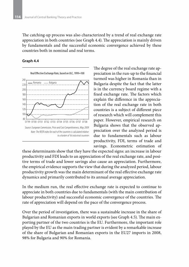
The catching-up process was also characterized by a trend of real exchange rate appreciation in both countries (see Graph 4.4). The appreciation is mainly driven by fundamentals and the successful economic convergence achieved by these countries both in nominal and real terms.

Graph 4.4

The degree of the real exchange rate ap-preciation in the run-up to the financial turmoil was higher in Romania than in Bulgaria despite the fact that the latter is in the currency board regime with a fixed exchange rate. The factors which explain the difference in the apprecia-tion of the real exchange rate in both countries is a subject of different piece of research which will complement this paper. However, empirical research on Bulgaria shows that the observed ap-preciation over the analyzed period is due to fundamentals such as labour productivity, FDI, terms of trade and savings. Econometric estimation of

these determinants show that they have the expected signs: an increase in labour productivity and FDI leads to an appreciation of the real exchange rate, and posi-tive terms of trade and lower savings also cause an appreciation. Furthermore, the empirical evidence supports the view that during the analyzed period, labour productivity growth was the main determinant of the real effective exchange rate dynamics and primarily contributed to its annual average appreciation.

In the medium run, the real effective exchange rate is expected to continue to appreciate in both countries due to fundamentals (with the main contribution of labour productivity) and successful economic convergence of the countries. The rate of appreciation will depend on the pace of the convergence process.

Over the period of investigation, there was a sustainable increase in the share of Bulgarian and Romanian exports in world exports (see Graph 4.5). The main ex-porting partner of the two countries is the EU. Furthermore, the important role played by the EU as the main trading partner is evident by a remarkable increase of the share of Bulgarian and Romanian exports in the EU27 imports in 2008, 98% for Bulgaria and 90% for Romania.


Graph 4.5

The two countries are also characterized by geographical diversification of their exports (see Graph 4.6).

Graph 4.6

As of 2008, the main exporting partners of Romania are Germany (16.4%), Italy (15.5%), France (7.4%) and Turkey (6.5%) (see Graph 4.7). As for Bulgaria, these are Greece (9.9%), Germany (9.1%), Turkey (8.8%) and Italy (8.4%) (see Graph 4.7), illustrating that during the analyzed period there is an improvement in the quality of exports in both countries as their exports are oriented towards de-


veloped countries which create entry opportunities for transition economies to progress on the quality ladder.

Graph 4.7

Product diversification is another important feature of Romanian and Bulgarian exports (see Graph 4.8).

Graph 4.8

The highest share of exports for both Romania and Bulgaria is occupied by ma-chinery and manufactured goods which further support the hypothesis that there is an improvement in the quality of exported goods during the analyzed


period. Although the share of machinery is higher in Romanian exports than in that of Bulgarian, the transition towards more technology intensive production in Bulgaria is evident and illustrated by the developments in two sectors – tex-tile and clothing, on one hand, and electrical equipment, electronics, transport equipment and other machinery on the other hand (the data cover short-term indicators of the National Statistical Institute). Textile industry decreased its share in total manufacturing exports in constant prices from 15% in 2004 to 11% in 2008. Exports of electrical equipment, electronics, transport equipment and other machinery grew from 16% in 2004 to 22% in 2008 and increased its exports between 2005 and 2008 by 85% in real terms.

5. Theoretical framework

There are several different methods of modelling demand for exports and im-ports. The appropriate model depends on different factors: whether the purpose of the model is hypothesis testing or forecasting; data availability and the level of disaggregation; and the type of traded goods. However, there are two general models of trade– perfect and imperfect - substitutes models. If the trade studies deal with aggregate imports (exports) the two models could be viewed as com-petitors. If however disaggregation is permitted the two models could be viewed as complements – one dealing with trade for differentiated goods, and the other with trade for close – if not – perfect substitutes.

The perfect -substitutes model

The following equations (5.1)-(5.8) below constitute a simple perfect substitutes model of trade for a representative country (i), outlined by Goldstein and Khan (1985):

l1 < 0 , l2 > 0 (5.1)

n1 > 0, n2 <0 (5.2)

(5.3)

(5.4)

(5.5)


(5.6)

(5.7)

(5.8)

In this perfect-substitutes model, Di is the total quantity of traded goods de-manded in country i; Si is the supply of traded goods produced in country i; Ii and Xi are the quantities of country i’s imports and exports; PIi, PXi, Pi and Pw are the import, export, domestic and world prices of traded goods; Dw and Sw are the world demand and supply of traded goods; and Yi and Fi are money income and factor costs in country i.

There are two main features of the perfect –substitutes model. First, there are no separate import and export demand functions. Instead, the demand for imports and the supply of exports represent the respective “excess” demand and “excess” supply for domestic goods; see eqs. (5.3) and (5.4). Second, when we abstract from transportation costs and other trade barriers (e.g. tariffs) and express all prices in a common currency, then there is only one traded goods price in the perfect-substitutes model (i.e. Pi = PIi = PXi = Pw). Furthermore, this (world) price is determined by the interaction of world supply and world demand for the traded good. The perfect-substitutes model is therefore more appropriate for modelling trade relationships of homogenous commodities (wheat, copper, sugar, etc.) that are traded on international commodity markets at a common price.

The imperfect - substitutes model

In equations (5.9-5.8) an imperfect substitutes model of country i’s imports from, and exports to, the rest of the world (*) outlined by Goldstein and Khan (1985) is presented:

f1,f3 > 0, f2 < 0 (5.9)

g1, g3 > 0, g2 < 0 (5.10)

h1 > 0, h2 < 0 (5.11)

j1 > 0, j2 < 0 (5.12)


(5.13)

(5.14)

(5.15)

(5.16)

These eight equations determine the quantity of imports demanded in country i (Ii

d), the quantity of country i’s exports demanded by the rest of the world (Xid),

the quantity of imports supplied to country i from the rest of the world (Iis), the

quantity of exports supplied from country i to the rest of the world (Xis), the

domestic currency prices paid by importers in the two regions (PIi and PI*), and the domestic currency prices received by exporters in two regions (PXi, PX*). The exogenous variables are the levels of nominal income in the two regions (Yi, Y*), the price of (all) domestically produced goods in the two regions (Pi, P*), the pro-portional tariff (Ti, T*) and subsidy rates (Si, S*) applied to exports and imports in the two regions, and the exchange rate (e) linking the two currencies (expressed in units of country i’s currency per unit of the rest-of-world’s currency).

The main characteristic of the model is that the consumer is postulated to maxi-mize utility subject to a budget constraint. The demand functions for imports and exports therefore represent the quantity demanded as a function of the level of (money) income in the importing region, the imported goods̀ own price, and the price of domestic substitutes. An additional assumption is often made that a consumer has no money illusion, so that the doubling of money income and all prices leaves demand constant, i.e. f1 + f2 +f3=0, g1 + g2 + g3=0. Such homogeneity of the demand function is expressed by dividing the right-hand side of eq. (5.9) by Pi, so that the two arguments of the demand function become the level of real income (Yi/Pi) and the relative price of imports (PIi/Pi). Accordingly, if we divide the right-hand side of eq. (5.10) by P*, the two arguments of the demand function for exports become the level of external demand (Y*/P*) and the relative price of exports (PXi/P*). These are the two equations that are usually estimated in empirical work modelling export and import of a given country. The prevailing practice is therefore to assume that the supply price elasticity for imports and ex-ports ( i.e. h1 in eq. (5.11) and j1 in eq. (5.12) respectively) for small economies are infinite, which allows satisfactory estimation of the import and export demand equations (5.9) and (5.10) by single-equation methods, since PIi and PXi can be viewed as exogenous.


The import and export demand functions for Bulgaria and Romania

The imperfect - substitutes model is more appropriate for the purpose of this paper due to the fact that neither exports nor imports are perfect substitutes for domestic goods. If domestic and foreign goods were perfect substitutes, then countries would specialize in either only importing or only exporting particular goods. In practice, however, both domestic and imported goods can be found coexisting in markets, indicating that countries do not in fact specialize to such a high degree.

Import demand functions

Studies by Khan and Ross (1977) and Salas (1982) suggest that in modelling an aggregate import demand function the log-linear specification is preferred to the linear formulation. The use of the log-linear formulation constrains the price and income elasticity estimates to be constant over the estimation period while the linear form of the import demand equation implies decreasing price elasticity and an income elasticity tending towards one.

Accordingly, following the imperfect-substitutes model, the long-run import de-mand function for Bulgaria and Romania is specified as follows:

m1>0, m2<0 (5.17)

where DD is domestic demand, IMP is the import deflator, GDP is the GDP defla-tor

Therefore, the demand for imports depends positively on domestic demand and negatively on the real exchange rate which is the relative price of import and GDP deflators.

Export demand functions

Following the imperfect-substitutes model, the following export demand func-tion for Bulgaria and Romania can be derived:

Xd=x(Yf, PXh, PXc) f1>0, f2<0, f3>0 (5.18)


where Xd= the quantity of the domestic good which is exported to the foreign market, Yf= the real foreign income, PXh=the price of the domestic good, PXc= the price of competing suppliers in a foreign market in a common currency, and fi=the expected partial derivatives of the export function with respect to the ith argument .

We also incorporate in the paper FDI in the export demand function to inves-tigate if it has a significant effect on export performance. Foreign direct invest-ments influence supply-side determinants of exports, reflecting to some extent the quality of physical capital as well as workers̀ skills and market penetration potential. The so-called New Trade Theory, influenced by the theory of industrial organization, has added this new insight into the possible factors affecting the demand for exports, such as FDI or the quality of traded goods. There are several papers that find a positive relationship between FDI and exports. Using aggregate data, Driver and Wren-Lewis (1999) derive a specification for exports that allows for traditional relative-price effects as well as effects from innovation in variety and quality. They estimate this model for the panel of the G-7 countries using time series and panel co-integration techniques. In addition, Pain and Wake-lin (1998) analyze the export performance and also relate foreign direct invest-ment to innovation in industries. They estimate conventional panel of 11 OECD countries specified as an error correction mechanism. Finally, Bajo and Montero (1995, 2001) estimate Spanish demand for exports using FDI and examine the causality relationship between FDI and trade. Based on the aforementioned ar-guments, equation (3.2) can be extended with the introduction of FDI stock as the proxy for quality:

Xd= x(Yf ,PXh, PXc, FDI), f4>0 (5.19)

The log-linearization of the equation (5.19) is:

x1>0, x2<0, x3>0 (5.20)

The equation above represents the long-term co-integrating relationship among exports and its determinants, illustrating that real exports depends positively on external demand, negatively on real exchange rate which is the ratio of home to competitor’s price, and positively on FDI stock which is the proxy for quality.


6. Data

All data are in real terms (2005=100 for Bulgaria and Romania). The data on real exports, real imports and domestic demand for Bulgaria are from the Bulgarian National Accounts of the Bulgarian National Statistical Institute. The data on real exports, real imports and domestic demand for Romania are from the Romanian Central Bank. The import, export, GDP and investment deflators for Bulgaria are from the Bulgarian National Statistical Institute. The import, export, GDP and investment deflators for Romania are from the Romanian Central Bank. The FDI accumulated inflows for Bulgaria are from the Bulgarian National Bank, they are in the national currency and investment in real estate is subtracted. The FDI accumulated inflows for Romania are from the Romanian Central Bank and they are also in the national currency. Manufacturing export price for advanced economies taken from the IMF is used as the proxy for external price for Bulgaria and Romania. However, it is in US dollars, so we convert it in the respective na-tional currencies by using the exchange rate Bulgarian lev per US dollar from the Bulgarian National Bank, and the exchange rate Romania lev per US dollar from Eurostat. The external demand of Bulgarian and Romanian exports is based on calculations of the OECD and the Bulgarian National Bank.

7. Empirical estimation and results

The empirical estimation includes four stages and employs Engle-Granger (1987) two step procedure. The four stages of the overall empirical estimation of the export and import demand functions of Bulgaria and Romania are as follows:

First, we determine the order of integration of the variables by deploying the Augmented Dickey-Fuller (ADF) and Phillips-Perron (PP) unit root tests. The PP test was designed to be robust for the presence of autocorrelation and heterosce-dasticity.

The regression equation for the ADF test (see Dickey and Fuller, 1979) is given as follows:

(4.1)

where Δ is first difference operator, t refers to time trend, and k is additional terms in the first differences for the Augmented Dickey-Fuller (ADF) test et is the regression error assumed to be stationary with zero mean and constant variance.


The Phillips Perron test is also based on equation (4.1) but without the lagged differences. Both tests were carried out to reject the null hypothesis of a unit root (c=0 for ADF, and c=1 for PP). The results are presented in Appendix I, and they show that all variables are integrated of order one, I(1), i.e. stationary in their first differences.

Second, we estimate the long-run equation which is the first step of the Engle-Granger two-step procedure.

Third, as we find that the variables are co-integrated (the error term is stationary, the results are in Appendix II), we specify error correction models and estimate them - this is the second step of the Engle-Granger two-step procedure. In the short run, we include four lags and non-significant lags are eliminated sequen-tially starting with the least significant one until only significant variables are left.

In the final step following Allard (2009), dynamic contributions are computed to assess the role of the various explanatory variables in the evolution of exports and imports over the period 2000-2008.

The results from the estimated equations are enclosed in Appendix III. The es-timated coefficients take the theoretically expected sign except for the short-run relative price for Romanian exports.

Table 7.1: Exports long-term elasticity related to non-price competitiveness

Bulgaria Romania

External demand 0.96 0.78

FDI accumulated inflows 0.20 0.19

Table 7.2: Exports long-term elasticity to price competitiveness

Bulgaria Romania

Relative price -0.08 -0.10

The pick up in external demand accounts for the largest part of growth in exports of Bulgaria and Romania over 2000-2008 (see Graph 7.1). This growth reflects the ability of smaller countries to expand their market share more systematically since transition, the result evident from the relatively high elasticity to external demand (the elasticity is higher in Bulgaria than in Romania).


The accumulated FDI investment also contributed positively to export growth, more in Bulgaria than in Romania. This illustrates that the quality of physical capital and workers̀ skills played a significant role in the export performance of the two economies. The EU accession also contributed to the attraction of new investors leading to more export-oriented new projects.

The price elasticity is low in both economies, however, it is slightly lower in Bul-garia than in Romania, possibly reflecting a different technology content of ex-port goods (for example, exports of high-technology goods are less price elastic). We could conclude that price competitiveness was not a problem for Bulgaria and Romania during the period of investigation. The relative prices had a slight nega-tive contribution in Bulgarian exports and almost no contribution in Romanian exports (see Graph 7.1). This result suggests that most of the trend appreciation of the real exchange rate in both countries is an equilibrium development, not a loss in price competitiveness.

The contribution of others (constant, seasonals and residual) for both countries is negative, although to a lesser extent in Bulgaria (see Graph 7.1). This could in-clude the overall business climate, the sectoral orientation of trade or non-price competitiveness indicators that are not captured in the estimation.

Graph 7.1


Graph 7.2

Concerning the imports, strong domestic demand played a key role for both countries as expected (see Graph 7.3). The elasticity of imports of both coun-tries to domestic demand is around two, illustrating high elasticity to domestic demand. The inelasticity of import with respect to import price in Bulgaria and Romania implies that during the period of investigation, imports were largely determined by non-price factors. By contrast with the export equations, the oth-er factors (constant, seasonals and residual) are positive which pushed up the growth rate of imports. This could include FDI, for example, which is not in-cluded in the estimation.

As import demand is income elastic in the long run, economic growth may have negative implications on the balance of payments in Bulgaria and Romania. In order to mitigate these negative effects, government strategies should promote the development of domestic capital goods industries and also industries that produce consumption and intermediate goods that are competitive in terms of price and quality to imports.

Table 7.3: Imports long-term elasticity related to non-price competitiveness

Bulgaria Romania

Domestic demand 2.29 1.63


Table 7.4: Imports long-term elasticity to price competitiveness

Bulgaria Romania

Relative price -0.20 -0.12

Graph 7.3

Graph 7.4


If we extend the sample to the fourth quarter of 2010, as the data are available to this date, a structural break occurs and the results are difficult to interpret. However, several important points could be emphasized for the period of the global economic crisis. While Bulgaria and Romania entered the period of global turmoil from a strong competitive position, their reliance on global and domes-tic demand had a negative impact on trade flows. The relatively high elasticity to external demand had a big impact on exports (the volume of Bulgarian ex-ports declined by 11.2% in 2009 and the volume of Romanian exports declined by 5.3%, supported by the empirical results that the Bulgarian exports have higher elasticity to external demand compared to the Romanian exports). Also, imports declined in both countries due to a decrease in domestic demand. Furthermore, the elasticity of imports to domestic demand are higher than elasticity to exter-nal demand which explains why imports declined by more than exports in both economies (the volume of the Bulgarian and Romanian imports declined respec-tively by 21% and 20.9% in 2009).

8. Conclusions

The paper provides insights in the trade determinants of Bulgaria and Romania which recently became EU members in the context of the convergence process and also in relation to different exchange rate regimes. The global and domestic acceleration explains a significant part of export and import developments in both countries during the period 2000-2008. The pickup in growth in the EU largely explains the exports growth in Bulgaria and Romania. This study also shows that over the period of investigation, Bulgaria and Romania were able to increase their market shares, partly due to strong FDI inflows.

The key conclusion is that price competitiveness does not appear to have a sig-nificant impact on trade developments in Bulgaria and Romania. Despite rapid exchange rate appreciation, which was more prominent in Romania than Bul-garia, although the latter is with a fixed exchange rate, relative prices remained muted. The evolution of relative price had a negligible negative contribution to the Bulgarian exports and almost no contribution to the Romanian exports. As for imports, the relative prices boosted imports for Romania and had a very small negative contribution for Bulgaria. These results suggest that most of the trend appreciation of the real exchange rate reflects a shift of an equilibrium value rath-er than a loss in price competitiveness.


Overall, we could conclude that the convergence process in respect to trade in both economies is similar over the period of investigation irrespective of their exchange rate regime, currency board or managed float.


Appendix I: Currency board arrangement in Bulgaria

The operation of the currency board in Bulgaria is based on three major princi-ples laid down in the Law on the BNB, namely: (1) a fixed exchange rate which as of the moment of the euro introduction is BGN 1.95583 per EUR 1; (2) the total amount of the BNB monetary liabilities is fully covered by full high-liquid foreign reserves. BNB monetary liabilities consist of banknotes and coins in cir-culation, liabilities vis-à-vis banks, the government and budget organizations, liabilities to other depositors (see Issue Department balance sheet on the BNB website); (3) the central bank’s obligation to unconditionally and irrevocably sell and purchase levs against euros at the exchange rate fixed by the Law on the BNB. These principles mean that the national currency is issued solely against provid-ing reserve currency at the fixed exchange rate.

The currency board and the fixed exchange rate are further protected by the fol-lowing provisions in the Law on the BNB:

(1) The BNB may not extend loans and guarantees in any form whatsoever, in-cluding through purchase of debt instruments, to the Council of Ministers, mu-nicipalities, as well as to other government and municipal institutions, organiza-tions and enterprises. This provision excludes the possibility, in order to support the government in financing budget expenditure, to issue the national currency beyond the limit corresponding to the currency board principles.

(2) The BNB may not provide credit to banks except in case of liquidity risk threatening to affect the banking system stability. The terms and procedure for extending this credit, and criteria for identifying the existence of liquidity risk are set by an ordinance of the BNB, and the credit is to be extended up to the amount exceeding the lev equivalent of gross international reserves vis-à-vis the total amount of the BNB monetary liabilities. This provision also excludes the possibility, in order to support the banks, to issue the national currency beyond the limit corresponding to the currency board principles.

(3) The BNB shall invest its gross international reserves in accordance with the principles and practices of prudent investment, with investments in securities being limited to liquid debt instruments satisfying the following requirements: debt instruments issued by foreign countries, central banks, other foreign finan-cial institutions or international financial organizations, whereof obligations are assigned one of the two highest ratings by two internationally recognized credit rating agencies, and which are payable in freely convertible foreign currency.


Rules for investing gross international reserves are also intended to protect the quality of assets in which these reserves are invested.

The above principles of the currency board operation guarantee an automatic mechanism of balancing national currency demand and supply at the fixed ex-change rate determined by the law. Under the currency board, it is impossible that the issue of national currency exceeds the level of the gross international foreign exchange reserves, which could, otherwise, lead to erosion of the fixed exchange rate (the key difference between a currency board and a standard fixed exchange rate regime). The change in the level of the BNB gross international reserves re-flects the net result of demand for the national currency by economic agents, gov-ernment and banks, as well as changes in the market value of gold (as part of international reserves) and financial assets in which these reserves are invested.

Under the conditions of the fixed exchange rate against the euro and a free move-ment of capital, the BNB has no control over the interest rates and therefore, monetary conditions in Bulgaria follow to a great extent those in the euro area. Thus, the currency board largely reproduces the conditions in which the Euro area economy is functioning.

The main instrument used by the BNB to affect monetary conditions is the regu-lation of the minimum required reserves maintained by banks with the central bank. For example, the reduction of the minimum required reserves rate since early 2009 has boosted liquidity in the banking system and contributed to falling interest rates in the interbank money market. It is possible for the central bank to indirectly influence the monetary conditions in Bulgaria by implementing su-pervisory and administrative measures, but their objective is mainly financial stability rather than affecting monetary conditions.

Fiscal policy may also affect money supply and liquidity in the economy through a change in the amount of the government deposit with the BNB, the net govern-ment securities issuance and their maturity or repurchases. Withdrawal of funds from the government deposit at the BNB and their depositing in other banks’ accounts could boost the banking system liquidity.

The implementation of these macroeconomic policy instruments affects the level of the international reserves. Any change in policies that lead to an increase of the required reserves that banks have to maintain with the BNB or fiscal policies that lead to increase in the government deposit with the BNB also lead to an increase of the international reserves and visa – versa. In this respect the fluctuations in the level of the international reserves are mainly policy driven.


Appendix II: Co-integration Tests

Table 1: Test results for unit roots for exports variables for Bulgaria

Variable ADF level First difference PP level First differenceLE_EX_R (exports) -0.962892 -2.548061* -2.468044 -11.02786*

LRP (relative price)

-2.344142 -4.089647* -2.696441 -4.153125*

LE_FDI_R (FDI)

-3.048278 -7.000493* -3.660610 -7.000493*

LA_WTV_R (ext. demand)

-2.274377 -1.777185 -1.464081 -6.218769*

*, ** and *** denote rejection of a unit root hypothesis based on MacKinnon’s critical value at 1 percent, 5 percent and 10 percent

Table 2: Test results for unit roots for import variables for Bulgaria

Variable ADF level First difference PP level First differenceLE_MP _R (imports) -1.23821 -3.003429** -7.016183* -22.99910*

LRELPR (relative price)

-1.679213 -6.251493* -1.561949 -6.243422*

LR_DD_R(dom. demand)

-0.667590 -4.110638* -9.228513* -16.01653*


Table 3: Test results for unit roots for residuals of export and import equations for Bulgaria

Variable ADF level PP levelResiduals (exports) -3.990354** -3.943055**

Residuals (imports) -3.347157** -3.359132**



Table 4: Test results for unit roots for exports variables for Romania

Variable ADF level First difference PP level First differenceLE_EX_R (exports) -1.718113 -8.893079* -4.087559** -10.51416*

LA_REER_R (real effective ER)

-1.428654 -4.683814* -1.512948 -4.742796*

LE_FDI_R (FDI)

-0.667553 -3.730669* -0.635338 -3.656584**

LA_WTV_R (ext. demand)

-3.267192 -3.991536* -3.838937** -7.376505*


Table 5: Test results for unit roots for import variables for Romania

Variable ADF level First difference PP level First differenceLE_MP _R (imports) -1.586173 -3.950805* -4.759125** -10.94347*

LRELPR (relative price)

1.091090 -1.453922 -3.720417** -7.452448*

LR_DD_R (dom. demand)

-2.067721 -1.938260 -7.289733* -12.84323*


Table 6: Test results for unit roots for residuals of export and import equations for Romania

Variable ADF level PP levelResiduals (exports) -3.271897** -3.080868**

Residuals (imports) -4.175699* -4.171295*



Appendix III: Estimated equations

Exports (Bulgaria)

ln(E_EX_R_STAR)=1.64+0.96ln(A_WTV_R)-0.08ln(E_EX_P/(A_MEPAE_P*A_ER_PI)+0.20*ln(E_FDI_N/R_KF_P)+seasonals

standard error of regression =0.05 DW=1.68 t statistics are in parentheses

dln(E_EX_R)=-0.96 - 0.78(ln(E_EX_R(-1)-ln(E_EX_R_STAR(-1)))+1.32dln(A_WTV_R)- (13.62) (3.66) (1.61) -0.21dln(E_EX_P/(A_MEPAE_P*A_ER_PI))+0.50dln(E_FDI_N/R_KF_P)+seasonals (1.41) (1.97)

Adj. R2=0.99 standard error of regression =0.05

where

E_EX_R – real exportsA_WTV_R – external demandE_EX_P – export deflatorA_MEPAE_P – competitor’s price in US dollarA_ER_PI – exchange rate BG currency per US dollarE_FDI_N – FDI accumulated inflows without real estate (nominal value)R_KF_P- Investment deflator

Exports (Romania)

ln(E_EX_R_STAR)=4.13+0.78ln(A_WTV_R)-0.10ln(E_EX_P/(A_MEPAE_P*A_ER_PI)+0.19*ln(E_FDI_N/R_KF _P)+seasonals


dln(E_EX_R)=0.07 - 0.18(ln(E_EX_R(-1)-ln(E_EX_R_STAR(-1)))+0.70dln(A_WTV_R)- (1.25) (1.39) (1.57)

+0.08dln(E_EX_P/(A_MEPAE_P*A_ER_PI))+0.17dln(E_FDI_N/R_KF _P)+seasonals (1.27) (1.37)



where

E_EX_R – real exportsA_WTV_R – external demandE_EX_P – export deflatorA_MEPAE_P – competitor’s price in US dollarA_ER_PI – exchange rate RO currency per US dollarE_FDI_N – FDI accumulated inflows without real estate (nominal value)R_KF_P- Investment deflator

Imports (Bulgaria)

ln(E_MP_R_STAR)=-10.81+2.29ln(R_DD_R)-0.20ln(E_MP_P/R_GDP_P)+seasonals


dln(E_MP_R)=-0.88 - 0.67(ln(E_MP_R(-1 ) -ln(E_MP_R_STAR(-1))) + 4.19dln(R_DD_R)- (20.86) (3.46) (1.47)

- 0.20dln(E_MP_P/R_GDP_P)+seasonals (1.75)


where

E_MP_R – real importsR_DD_R – domestic demandE_MP_P – import deflatorR_GDP_P – GDP deflator

Imports (Romania)

ln(E_MP_R_STAR)=-7.44+1.63ln(R_DD_R)-0.12ln(E_MP_P/R_GDP _P)+seasonals


dln(E_MP_R)=-0.11 - 0.78(ln(E_MP_R(-1 ) -ln(E_MP_R_STAR(-1))) + 0.99dln(R_DD_R)- (1.45) (2.53) (2.06)

- 0.27dln(E_MP_P/R_GDP_P)+seasonals (1.47)



where

E_MP_R – real importsR_DD_R – domestic demandE_MP_P – import deflatorR_GDP_P –GDP deflator


Appendix IV: Principle of dynamic contributions8

Let Yt be the endogenous variable, Xi the explanatory variables, and εt the econo-metric residual.

The ECM can be written as (1)

where is determined by the co-integration relation-ship.

Breakdown by explanatory variables

The estimated full dynamic can be summarized as

where L is the lag operator, and A(L) and Bi(L) polynomials of this lag operator.

From (1), and

By inverting A(L), one gets:

The dynamic contributions of variables Xi to the growth rate of variable Y are then derived (additively) from the differentiation of (1):

(2)

This breakdown also allows one to visualize what remains unexplained in the econometric relationship, through the contributions of the residuals.

Breakdown between short- and long- term dynamics

Another presentation consists of distinguishing between the contribution of the short-term dynamic, through all the variables in growth rate in equation (1), and the long-term dynamic, through the impulse from the error-correcting term:

8 It follows Allard (2009).


where

By inverting A*(L), one gets:

(3)

The first two elements on the right side of (3) – the constant and the terms with the growth rate of Xi variables – correspond to the contribution of the short-term dynamic, whereas the term with the error-correcting factor shows the contribu-tion of the long-term dynamic namely, by how much the gap from the steady state equilibrium contributes to the growth rate of variable Y. Here again the break-down also allows one to visualize what remains unexplained in the econometric relationship, through the contribution of the residuals.


References

1. Adam, C. and D. Cobham (2007). Exchange rate regimes and trade. The Man-chester School, 75, 1, 44-63.

2. Algieri, B. (2004). Price and income elasticities for Russian exports. The Eu-ropean Journal of Comparative Economics, 1(2), 175-193.

3. Allard, C. (2009). Competitiveness in Central Europe: What has happened since EU accession?. IMF Working Paper.

4. Bajo, O. and M. Montero (2001). Foreign direct investment and trade: a cau-sality analysis. Open Economies Review, 12, 305-323.

5. Brenton, P. (1999). The impact of the next enlargement. CEPS, Brussels. 6. Carone, G. (1996). Modelling the US demand for imports through co-inte-

gration and error correction. Journal of Policy Modelling, 18(1), 1-48.7. Cubadda, G., S. Fachin and F. Nucci (1999). Disaggregated Import Demand

Functions for the Italian Economy , in Sardoni, C. and P. Kriesler (eds.), Keynes, Post-Keynesisanism and Political Economy, Esseys in Hounour of Geoff Harcourt, 3, 510-526.

8. Dickey, D. A. and W. A. Fuller (1979). Distribution of the estimators for au-toregressive time series with a unit root. Journal of the American Statistical Association, 74, 427-431.

9. Driver, R. and S. Wren-Lewis (1999). New trade theory and aggregate export equations: an application of panel co-integration. Discussion Paper in Eco-nomics, University of Exeter.

10. Funke, M. and R. Ruhwedel (2001). Export variety and export performance: empirical evidence from East Asia. Journal of Asian Economics, 12, 493-505.

11. Goldstein, M. and M.S. Khan (1978) . The supply and demand for exports: a simultaneous approach. Review of Economics and Statistics, 60, 275-286

12.Goldstein, M. and M.S. Khan (1985). Income and price effects in foreign trade. in R.W.Jones and P.B.Kenen (eds.), Handbook of International Economics, II.

13.Harvylyshyn, O. and H. Al-Atrash (1988). Opening up and geographic diver-sification of trade in transition economies. IMF Working Paper.

14.Houthakker, H. S. and S.P. Magee (1969). Income and price elasticities in world trade. Review of Economics and Statistics, 41, 111-25.

15. Khan, M.S. and K.Z. Ross (1977). The functional form of the aggregate im-port equation. Journal of International Economics, 7, 149-60.

16.Klein, M. and J.C. Shambaugh (2006). Fixed exchange rates and trade. Jour-nal of International Economics, 70, 359-383.

17. Krugman, P. (1989). Differences in income elastictities and trends in real ex-change rates. European Economic Review, 33, 5, 1031-54.


18.Krugman, P. and M. Obstfeld (1997). International Economics. Theory and Policy. Addison-Wesley.

19. Lin, A. (1995). Trade effects of foreign direct investment: evidence for Taiwan with four ASEAN countries. Weltwirtchaftliches Archiv 131, 737-747.

20.Murray, T. and P.J. Ginman (1976). An Examination of the traditional ag-gregate import demand model. Review of Economics and Statistics, 58, 75-80.

21. Pain, N. and K. Wakelin (1998). Export performance and the role of foreign direct investment. The Manchester School Supplement, 62-88.

22.Rose, A.K. (2000). One money one market: estimating the effect of common currencies on trade. Economic Policy, 15, 7-46.

23. Salas, J (1982). Estimation of the structure and elasticities of Mexican imports in the period 1961-1979. Journal of Development Economics, 10, 297-311.

Documents

Trade, convergence and exchange rate regime: evidence · PDF fileTrade, convergence and exchange rate regime: ... Journal of Central Banking Theory and Practice, ... convergence and