Work ing PaPer Ser ieSno 1547 / may 2013

Current aCCount reverSalSin induStrial CountrieS

doeS the exChangerate regime matter?

Cosimo Pancaro

In 2013 all ECB publications

feature a motif taken from

the €5 banknote.

note: This Working Paper should not be reported as representing the views of the European Central Bank (ECB). The views expressed are those of the authors and do not necessarily reflect those of the ECB.

© European Central Bank, 2013

Address Kaiserstrasse 29, 60311 Frankfurt am Main, GermanyPostal address Postfach 16 03 19, 60066 Frankfurt am Main, GermanyTelephone +49 69 1344 0Internet http://www.ecb.europa.euFax +49 69 1344 6000

All rights reserved.

ISSN 1725-2806 (online)EU Catalogue No QB-AR-13-044-EN-N (online)

Any reproduction, publication and reprint in the form of a different publication, whether printed or produced electronically, in whole or in part, is permitted only with the explicit written authorisation of the ECB or the authors.This paper can be downloaded without charge from http://www.ecb.europa.eu or from the Social Science Research Network electronic library at http://ssrn.com/abstract_id=2259549.Information on all of the papers published in the ECB Working Paper Series can be found on the ECB’s website, http://www.ecb.europa.eu/pub/scientific/wps/date/html/index.en.html

AcknowledgementsI would like to thank Kenza Benhima, Simone Bertoli, Giancarlo Corsetti, Harris Dellas, Marcel Fratzscher, Helmut Luetkepohl and Rasmus Rueffer for their valuable comments. However, I am solely responsible for any errors that remain. I am particularly grateful to Christian Saborowski for his extensive help. The findings, views and interpretations expressed herein are those of the author and should not be attributed to the ECB, its Executive Board, or its management.

Cosimo PancaroEuropean Central Bank; e-mail: cosimo.pancaro@ecb.europa.eu

Abstract

This paper studies current account reversals in industrial countries across different exchange

rate regimes. There are two major findings which have important implications for industrial

economies with external imbalances: first, triggers of current account reversals differ between

exchange rate regimes. While the current account deficit and the output gap are significant

predictors of reversals across all regimes, reserve coverage, credit booms, openness to trade

and the US short term interest rate determine the likelihood of reversals only under more

rigid regimes. Conversely, the real exchange rate affects the probability of experiencing a

reversal only under flexible arrangements. Second, current account reversals in advanced

economies do not have an independent effect on growth. This result holds not only for

industrial economies in general but also for countries with fixed exchange rate regimes in

particular.

Keywords: Current account, reversals, exchange rate regime

JEL Classification: F32, F41

Non-Technical Summary

Sharp external adjustments that lead to a sustained current account improvement are com-

monly referred to as current account reversals. Reversals have been analyzed intensively in

the literature, typically with a focus on the channels through which they are achieved as well

as on the question whether they have implications for real economic performance. However,

one aspect that has received only limited attention is the relationship between current account

reversals and exchange rate regimes, an aspect that is especially timely with regard to the ex-

isting external imbalances within the Euro area. The present paper contributes to this strand

of the literature by presenting a systematic analysis of current account reversals across different

de-facto exchange rate regimes in industrial countries. In particular, it examines whether cur-

rent account reversals follow different patterns depending on the exchange rate regime in place.

Moreover, it identifies triggers of reversals and examines the link between reversals and growth

across different exchange rate regimes. The analysis focuses precisely on distinguishing rigid

exchange rate regimes from those that are more flexible when identifying triggers of reversals

and when analyzing the link between reversals and growth.

The paper proceeds as follows: we initially identify 43 episodes of current account reversals in

22 industrial economies between 1970 and 2007. The episodes are then grouped by types of de-

facto exchange rate regime. In particular, we distinguish three groups of exchange rate regimes:

fixed exchange rate regime, intermediate exchange rate regime and flexible exchange rate regime.

Then, a brief event study examining the average patterns of some key macroeconomic variables

before and after the reversal sets the stage for the empirical analysis which is split into two

parts. In the first part, we estimate a Probit model for the sample as a whole and, separately,

for each of the groups of exchange rate regimes in an effort to identify predictors of current

account reversals. We find that larger deficits and larger output gaps are associated with a

higher probability of experiencing reversals across all exchange rate regimes. Conversely, lower

reserves growth, higher domestic credit growth, higher US interest rates and a more closed

economy raise the probability of a reversal only under less flexible exchange rate regimes. A

real exchange rate depreciation, on the other hand, is a significant trigger only under flexible

regimes. In the second part of the study, we estimate a treatment effects model to test whether

sharp current account corrections negatively affect growth both for the sample as a whole and,

separately, for different types of exchange rate regimes. In anticipation of our results, we find

no evidence in favor of this hypothesis, neither for the sample as a whole nor for the subsample

of fixed exchange rate regimes.

2

1 Introduction

The years preceding the global crisis saw large and persistent current account imbalances which

peaked at some three percent of global GDP in 2006 (IMF 2012a). Commentators focused

primarily on the US deficit, but many other advanced economies including Australia, Greece,

Ireland, New Zealand, Portugal and Spain recorded large and persistent external deficits at that

time. After the outbreak of the financial crisis, several world economies experienced sizable

current account corrections, yet the intense debate among academics and policy-makers about

the nature and the sustainability of global current account imbalances continues (Feldstein 2008;

Obstfeld 2012; Serven and Nguyen 2010)1. While external positions can often be explained

by economic fundamentals such as demographics or expectations of productivity growth, the

pronounced imbalances recorded prior to the crisis reflected at least in part structural distortions

such as unsustainable expansionary fiscal policies and asset booms in major advanced economies.

The perceived sustainability of these deficits determines whether and how long they can be

maintained and financed. Indeed, a current account deficit investors are no longer willing to

finance will be forced to reverse partly or fully, often within a short period of time (Blanchard

and Milesi Ferretti 2010; IMF 2012a).

Sharp external adjustments that lead to a sustained current account improvement are com-

monly referred to as current account reversals. Reversals have been analyzed intensively in the

literature, typically with a focus on the channels through which they are achieved as well as on

the question whether they have implications for real economic performance. However, one as-

pect that has received only limited attention in the literature is the relationship between current

account reversals and exchange rate regimes, an aspect that is especially timely with regard to

the existing external imbalances within the Euro area. To our knowledge only Edwards (2004a),

Edwards (2004b), De Haan, Schokker and Tcherneva (2008), Gosh, Terrones and Zettelmeyer

(2010), Chinn and Wei (2013) and Lane and Milesi-Ferretti (2012) have dealt with this im-

portant topic2. The present paper contributes to this strand of the literature by presenting a

systematic analysis of current account reversals across different de-facto exchange rate regimes.

In particular, it examines whether current account reversals in industrial economies follow dif-

ferent patterns depending on the exchange rate regime in place. Moreover, it identifies triggers

of reversals and examines the link between reversals and growth across different exchange rate

regimes.

Milesi-Ferretti and Razin (2000) is one of the first among a growing number of studies that

1In 2008, current account deficits amounted to 4.4% of GDP in Australia, 14.9% in Greece, 5.7% in Ireland,8.8% in New Zealand, 12.6% in Portugal, 9.6% in Spain and 4.7% in the US. These are largely unprecedentedamong industrial countries. In 2011, as a percentage of GDP, the current account deficit reached 2.3% in Australia,9.8% in Greece, -1.1% in Ireland, 4.2% in New Zealand, 6.4% in Portugal, 3.5% in Spain and 3.1% in the US(IMF 2012b).

2Chinn and Wei (2013) assess whether ‘The Case for Flexible Exchange Rates’ made by Friedman in 1953is supported by any empirical evidence. Indeed, they systematically study the relationship between de-factoexchange rate regimes and the speed of current account reversion. Lane and Milesi-Ferretti (2012) examine theprocess of adjustment of external imbalances between 2008 and 2010 considering both a large sample of countriesand 2 sub-samples defined according to the countries’ de-facto exchange rate regimes.

3

explicitly analyzes the triggers and patterns of current account reversals. The authors use a

large panel of developing countries to identify determinants of current account reversals. The

evidence suggests that the current account balance itself, a country’s openness to trade, its

terms of trade and reserve coverage as well as growth in industrial economies and US interest

rates are drivers of current account reversals in developing economies. Moreover, conducting a

before-after analysis, they do not find any evidence of a systematic relationship between current

account corrections and economic performance.

Freund (2005) was the first to systematically examine current account reversals in industrial

economies. Studying the patterns of macroeconomic variables during reversal episodes, she

finds that reversals in industrial economies are generally accompanied by a depreciation of the

real exchange rate, a decline in GDP growth, investment and imports, and a rise in exports.

The current account deficit takes between 3 and 4 years to resolve. Moreover, Freund (2005)

shows that a larger current account deficit and weakening growth are significant predictors of

reversals. However, she does not condition the triggers of reversals directly on the exchange rate

regime in place. De Haan et al. (2008) is the only study we are aware of that does take the role

of exchange rate regimes into account when analyzing triggers of current account reversals in

advanced economies. The authors find that, under a peg and a moving band, a deeper current

account deficit has less predictive power of current account reversals than under a crawling peg.

Conversely, a larger output gap has a lower predictive power under a moving band than under a

crawling peg. The authors do not, however, systematically distinguish groups of countries with

different exchange rate regimes as we do in this paper.

Croke, Kamin and Leduc (2006) study the link between current account reversals and eco-

nomic growth in industrial economies. Their work tests the so called “disorderly correction

hypothesis” which claims that current account reversals lead to a disruptive adjustment process

that translates into a decline in growth. While some current account reversals indeed coincide

with growth declines, the authors do not find any supportive evidence for a causal link between

the reversal itself and the fall in growth. Debelle and Galati (2007) come to the same conclu-

sion.3 However, the inability of these studies to identify a link between reversals and growth

may be due to the fact that they do not distinguish countries with fixed from those with more

flexible exchange rate regimes.

Indeed, Friedman (1953) already pointed out that flexible exchange rates allow a more

orderly adjustment process by functioning as external shock absorbers, i.e. by providing a

device for continuous adjustment and guaranteeing full autonomy to domestic policy in the

achievement of its targets. However, Chinn and Wei (2013) study the relationship between the

exchange rate regimes and the speed of current account adjustment and do not find any evidence

supporting the hypothesis that the current account reversion to its long run equilibrium is faster

3Debelle and Galati (2007) analyze the behavior and the role of financial flows and their composition duringreversals in industrial countries. Their results show that the more volatile types of flows, which are more stronglyaffected by changes in interest rates, are those that adjust the most. However, the dynamics of financial flowsdo not change significantly before a current account adjustment and their role in triggering a reversal does notseem to be relevant.

4

under flexible exchange rate regimes. This result suggests that current account imbalances are

not more persistent under fixed exchange rates. Indeed, in principle, fixing the nominal exchange

rate does not necessarily limit the ability of the real exchange rate to adjust, given sufficient

flexibility in prices and costs. However, in practice, both prices and wages are relatively sticky

compared to the nominal exchange rate. Thus, a fixed exchange rate regime may imply that

most of the adjustment burden has to be borne by changes in economic activity, potentially

leading to a more pronounced slowdown. Indeed, Edwards (2004a) and Edwards (2004b) find

in a sample of mainly developing economies that current account reversals lead to lower GDP

growth only under hard pegged and intermediate exchange rate systems.

The analysis in the present paper focuses precisely on distinguishing rigid exchange rate

regimes from those that are more flexible when identifying triggers of reversals and when an-

alyzing the link between reversals and growth. The paper proceeds as follows: we initially

identify 43 episodes of current account reversals in 22 industrial economies between 1970 and

2007. The episodes are then grouped by exchange rate regime using the de-facto classifica-

tion by Ilzetzki, Reinhart and Rogoff (2008)45. In particular, as in Chinn and Wei (2013), we

distinguish three groups of exchange rate regimes: fixed exchange rate regime, intermediate

exchange rate regime and flexible exchange rate regime. Then, a brief event study examining

the average patterns of some key macroeconomic variables before and after the reversal sets

the stage for the empirical analysis which is split into two parts. In the first part, we estimate

a Probit model for the sample as a whole and, separately, for each of the groups of exchange

rate regimes in an effort to identify predictors of current account reversals. We find that larger

deficits and larger output gaps are associated with a higher probability of experiencing rever-

sals across all exchange rate regimes. Conversely, lower reserves growth, higher domestic credit

growth, higher US interest rates and a more closed economy raise the probability of a reversal

only under less flexible exchange rate regimes. A real exchange rate depreciation, on the other

hand, is a significant trigger only under flexible regimes. In the second part of the study, we

estimate a treatment effects model to test whether sharp current account corrections negatively

affect growth both for the sample as a whole and, separately, for different types of exchange rate

regimes. In anticipation of our results, we find no evidence in favor of this hypothesis, neither

for the sample as a whole nor for the subsample of fixed exchange rate regimes.

The remainder of this paper is structured as follows: Section 2 outlines our identification

strategy for current account reversals and discusses the dynamics of key macroeconomic vari-

ables before and after the reversal. Section 3 presents our findings as regards the triggers of

current account reversals while Section 4 discusses the treatment effects model and our findings

related to the link between reversals and growth. Section 5 presents a battery of robustness

checks, and Section 6 concludes.

4Ilzetzki et al. (2008) provide updates to the de-facto exchange rate regime classification originally suggestedby Reinhart and Rogoff (2004).

5Following Edwards (2004a), Edwards (2004b), a given country is assigned the exchange rate regime in placefour quarters before the reversal starts. This strategy aims at addressing the effects of a potential regime switchon the results of the analysis

5

2 The dynamics of the current account adjustments: data and

event study

The analysis uses quarterly data from 1970 to 2007 for a sample of 22 industrial economies6.

Whenever quarterly data are not available for a given variable, we use annual data interpolated

to quarterly frequency.7 Episodes of current account reversals are identified using criteria similar

to those used in Algieri and Bracke (2011). The intention behind these criteria is to ensure that

episodes are only classified as reversals if periods of current account deficits are followed by

sustained improvements in current accounts. Specifically, an episode qualifies as a reversal if

the following 4 conditions are satisfied:

1. The current account is negative when the reversal starts.8

2. The annual average of the current account to GDP ratio improves by at least 1 standard

deviation by the third year after the reversal started.9

3. The maximum current account deficit in the 5 years after the reversal started is smaller

than the initial one.

4. There is no current account reversal in the 3 years before the reversal starts.

We identify 43 episodes of current account reversals based on these criteria. As can be seen

in Table A.6, most of the reversals occurred in the 1980s and in the 1990s, respectively 20 and

14 episodes. Only 6 reversals took place in the 1970s, a period of relatively limited financial

market and trade integration in advanced economies. Only 3 reversals have taken place since

200010. Figures A.2 and A.3 illustrate the incidence of current account reversals by country

and over time.

We group reversal episodes according to the de-facto exchange rate regime in place four

quarters before the reversal begins. This strategy allows addressing possible effects of regime

switches on the estimation results (Edwards 2004a,b)11. Following Chinn and Wei (2013), we

define three groups of exchange rate regimes: the fixed exchange rate regime corresponds to

the first 4 categories of the fine grid in Reinhart and Rogoff (2004) and ranges from “no legal

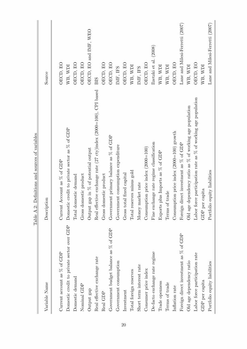
6A list of the countries in the sample is reported in Table A.1. Table A.2 shows a detailed description of thevariables we use as well as their sources.

7We used a linear interpolation method as part of which the last observation was matched to the source data.8As Algieri and Bracke (2011) and IMF (2007) highlight, this criterion allows for a larger sample size compared

to approaches that require the initial current account deficit to exceed a given magnitude. In a robustness check,we restrict the sample to reversals with an initial deficit larger than 2% of GDP as in Freund (2005) and findthat our main results are qualitatively unchanged.

9As in Algieri and Bracke (2011), we use the country specific standard deviation rather than a fixed thresholdin order to take account of country heterogeneity in current account dynamics. The highest current accountstandard deviation is in Norway (7.8%) while the lowest in France (1.2%)

10Based on the criteria used to identify reversals, the last year in which an episode could have taken place inour sample is 2002.

11There are only 2 cases of reversal episodes in which regime switches took place during the four quartersleading up to the starting point of the reversal. These are the reversals in Greece 1985q3 and Greece 1990q1.

6

tender” to “de facto peg”; the intermediate exchange rate regime includes the categories 5 to

11 and ranges from “pre-announced crawling band that is narrower than or equal to +/-2%” to

“noncrawling band that is narrower than or equal to +/-2%”; finally, the flexible exchange rate

regime comprises categories 12 and 13 and comprises “managed floating” and “freely floating”.12

Observations that correspond to a “freely falling” de-facto regime are dropped13. Figures A.4

and A.5 show countries’ de-facto exchange rate regimes, as well as how these changed over time.

We find that, of the 43 episodes in our sample, 7 took place under fixed exchange rate regimes14,

22 under intermediate exchange rate regimes and 14 under flexible exchange rates. Therefore,

current account reversals occurred with the highest likelihood under the intermediate exchange

rate regimes and with the lowest probability under fixed exchange rate regimes. Table A.6

reports the distribution over time of the de-facto exchange rate regime observations in the sample

and shows that the intermediate exchange rate regime observations are the most represented

category in the sample while flexible exchange rate regimes are least represented.

Figure 1 illustrates the average patterns of key macroeconomic variables including the cur-

rent account as % of GDP, economic growth, the output gap as % of potential output, domestic

demand growth, the government balance as % of GDP and the real effective exchange rate

during episodes of current account reversals for each group of exchange rate regime in the 24

quarters surrounding the current account trough. Several important observations can be made.

First, the charts suggest that current account reversals are typically preceded by a significant

deterioration of the current account. While patterns are generally similar across exchange rate

regimes, there are notable differences in the magnitude of the average deficit attained in the

year of the reversal. In particular, the trough occurs on average at -6% of GDP for flexible

exchange rate regimes and at -4% for fixed regimes (Table A.7). Following a rapid improvement

in the subsequent years, the current account is in balance again for all regimes after about three

years. The dynamics of the trade balance (not shown) reflect those of the current account. The

trade balance deficit in the trough is smaller than the current account deficit and varies between

3.2% of GDP under flexible exchange rates and 1.6% of GDP under fixed exchange rates. As

expected, trade developments explain a good share of the overall current account deficit.

Second, the main driver of the current account reversals in our sample is a dramatic drop

in domestic demand growth, in line with Algieri and Bracke (2011), IMF (2005, 2006) and

others who find that large current account adjustments tend to occur through marked changes

in the overall volume of expenditure rather than expenditure switching. The drop in domestic

demand leads to a significant contraction in economic activity. Growth reaches its trough

between 3 (fixed and intermediate) and 8 (flexible) quarters following the start of the reversal.

12Table A.3 reports the fine grid provided by Reinhart and Rogoff (2004) while Table A.4 shows our exchangerate regime classification which follows Chinn and Wei (2013).

13The dropped observations are: Finland 1992q4 and 1993q1, Italy 1992q4 and 1993q1, Korea 1998q1 and1998q2.

14Given that 5 out of 7 of the reversals which occured under fixed exchange rate regimes took place in EMUcountries - albeit at different stages of the monetary integration process - the results for the fixed exchange rateregime group could potentially reflect characteristics specific to EMU currency arrangements.

7

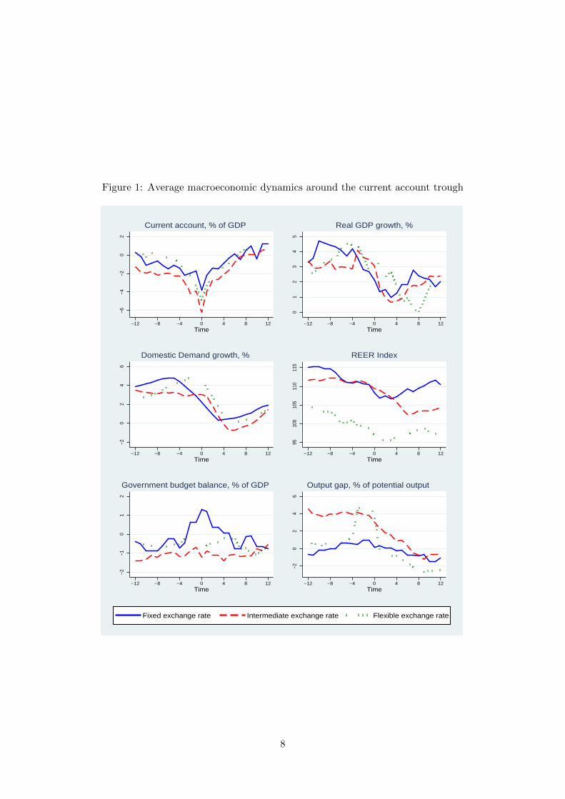
Figure 1: Average macroeconomic dynamics around the current account trough

−6−4

−20

2

−12 −8 −4 0 4 8 12Time

Current account, % of GDP

01

23

45

−12 −8 −4 0 4 8 12Time

Real GDP growth, %

06

42

−2

−12 −8 −4 0 4 8 12Time

Domestic Demand growth, %

9510

010

511

011

5

−12 −8 −4 0 4 8 12Time

REER Index

−2−1

01

2

−12 −8 −4 0 4 8 12Time

Government budget balance, % of GDP

−20

24

6

−12 −8 −4 0 4 8 12Time

Output gap, % of potential output

Fixed exchange rate Intermediate exchange rate Flexible exchange rate

8

Interestingly, more flexible exchange rate regimes do significantly better in the first year after

the reversal but do worse in the second year. One reason for this finding could be that, in our

sample, the average country with a reversal episode under fixed exchange rates is significantly

more open to trade than its counterparts with more flexible regimes.15

Third, the output gap mirrors the dynamics of growth, suggesting that the state of the

economy relative to trend may be an important leading indicator for reversals. The output

gap reaches its maximum (i.e. the largest gap between actual and potential GDP) just before

the adjustment starts and subsequently begins to decline. Interestingly, the output gap shows

the largest pre-reversal spike in the case of flexible exchange rate regimes, perhaps reflecting

the fact that nominal exchange rate depreciation prior to the reversal fosters a more significant

overheating. The real depreciation begins before the current account reversal takes place and

continues for a few quarters following the reversal. On average, the depreciation is largest under

flexible exchange rates.

Finally, the average dynamics of the government budget balance under fixed exchange rate

regimes largely differ from those under more flexible arrangements. While a budget balance

consolidation anticipates the current account adjustment under fixed exchange rates, it remains

largely unchanged under other types of regimes. Fixed exchange rate regimes appear to impose

a stricter fiscal discipline. This contributes to keeping the output gap in check.

3 Predictors of current account reversals

We proceed to identify determinants of current account reversals based on a Probit model.

We estimate the model separately for the sample as a whole and the three groups of exchange

rate arrangements16. We find that the triggers of current account reversals indeed differ across

exchange rate regimes.

In the empirical literature, the predictors of reversals are typically identified by way of

estimating a binomial discrete choice model where the dependent variable is equal to 1 in the

quarter in which the current account reversal starts and 0 otherwise. These models are aimed

at estimating how the likelihood of a reversal at a given point in time is affected by variation

in the covariates. However, such models are often characterized by a low capacity to identify

statistically significant predictors due to the limited number of current account reversals in

industrial countries in recent decades.17 In order to overcome this shortcoming, this paper

estimates a Probit model with a forward dependent variable. The forward dependent variable

15Countries with flexible regimes have average trade to GDP ratios of 38% and export to GDP ratios of 19%compared to 64% and 32%, respectively, in the case of less flexible regimes.

16We also experimented with estimating an augmented model with interaction terms between exchange rateregime dummies and the explanatory variables in place of the sample splits. However, the limited number ofdegrees of freedom does not allow including more than a small number of interaction terms at a time. This seemsproblematic in the present setup given that the entire data generating process may be considered conditionalupon the exchange rate regime in place

17De Haan et al. (2008) identify 41 episodes, but their sample is very heterogeneous and even includes episodesprior to the end of the Bretton Woods system. Freund (2005) identifies only 25 episodes.

9

is equal to one not only in the quarter when the current account adjustment starts but also

in the 4 quarters before; otherwise, it is equal to 0. This approach is used by Bussiere and

Fratzscher (2006) in the context of early warning models for predicting financial crisis. The

strategy increases the model’s capacity to identify statistically significant determinants in the

regressions and allows attenuating potential endogeneity concerns. On the downside, the model

does not explain the precise point in time in which a reversal begins but rather determines

whether an adjustment is more likely to occur within a given one year time window.

Our preferred specification is reported in Table 1 while the inclusion of additional controls is

discussed in the robustness section. Our choice of explanatory variables is in line with existing

studies in the literature (Freund 2005; Milesi-Ferretti and Razin 1998), and includes the current

account, the output gap, reserves growth, the real effective exchange rate, credit to the private

sector, trade openness and the US interest rate. Country dummies are also included but not

reported in the tables18. Table 1 illustrates the estimation results.

The findings suggest that a larger current account deficit is linked to a higher likelihood

of a current account reversal, irrespective of the exchange rate regime in place. This result is

unsurprising in that it suggests that the likelihood of current account sustainability is linked to

investors’ willingness to lend as the deficit grows (Milesi-Ferretti and Razin 1998). Similarly,

the output gap is a significant predictor of reversals under all exchange rate arrangements: a

larger output gap is associated with a higher likelihood of a reversal. Intuitively, the result

suggests that reversals occur when an economy is overheating, signalling that domestic demand

is overstretching the productive capacity of the economy.

A number of explanatory variables explain current account reversals under fixed or interme-

diate exchange rate regimes while they cannot be identified as significant determinants under

flexible exchange rates.

First, a decline in foreign reserves leads to a higher likelihood of a reversal - in line with sol-

vency and willingness to lend considerations (Milesi-Ferretti and Razin 1998) - only in countries

with fixed and intermediate exchange rate regimes. This result is as expected since reserves are

needed to defend tightly managed exchange rates in the presence of potentially large capital

outflows while the same is not the case under flexible exchange rate regimes.

Second, increases in private credit significantly raise the likelihood of current account rever-

sals under more rigid exchange rate regimes. Intuitively, under fixed exchange rates, a credit

expansion may exacerbate inflationary pressures leading to an overvaluation of the currency as

the nominal exchange rate cannot adjust. Such overvaluation may trigger a drain of foreign

reserves, reduce the competitiveness of domestic products, aggravate the current account deficit

and thus raise doubts about its sustainability. In contrast, under flexible exchange rate regimes,

credit growth is not a significant trigger of reversals. Intuitively, its inflationary effects will not

necessarily lead to an overvaluation as the nominal exchange rate can adjust.

Third, the analysis finds that an increase in the US interest rate - an indicator of the

18Time dummies were excluded due to joint insignificance based on an F-test.

10

international cost of borrowing - leads to a higher probability of a reversal under fixed exchange

rate. Intuitively, a rise in the international cost of borrowing diminishes a country’s ability to

finance its current account deficit. This is true especially in economies with a fixed exchange

rate and an open capital account in which monetary policy is not fully independent. Hence, an

increase in the international cost of borrowing forces domestic interest rates to rise and domestic

demand to contract potentially triggering a reversal.

Finally, an increase in the degree of trade openness also reduces the probability of current

account reversals only under non-freely floating exchange rate regimes. Intuitively, countries

with larger export sectors can more easily service external debt due to the larger amount of

export proceeds, thus attenuating sustainability concerns.

In contrast, the real effective exchange rate is a significant predictor of current account

reversals only in the cases of flexible regimes. In particular, exchange rate depreciation signifi-

cantly raises the probability of a reversal to occur in such episodes. This result is in line with

the graphical analysis which shows that the real depreciation that tends to anticipate current

account reversals is more pronounced under flexible arrangements.

A Chow test confirms that the coefficient estimates are indeed significantly different from

each other between the three subsamples.

Table 1: Probit model: triggers of current account reversals by exchange rate regime

Fixed Intermediate Flexible Wholeexchange exchange exchange samplerate regime rate regime rate regime

(1 ) (2 ) (3 ) (4 )

Current account as % of GDP -0.576*** -0.144*** -0.0820** -0.157***(0.130) (0.0249) (0.0333) (0.0179)

Output gap 0.492*** 0.0392* 0.286*** 0.0797***(0.146) (0.0210) (0.0661) (0.0153)

Total reserves growth -2.170*** -0.395* 0.150 -0.193(0.746) (0.217) (0.291) (0.156)

Real effective exchange rate 0.0331 -0.00962 -0.0302** -0.0218***(0.0374) (0.00965) (0.0125) (0.00583)

Domestic credit to private sector over GDP 0.114*** 0.00907** -0.00192 0.000778(0.0313) (0.00436) (0.00472) (0.00237)

Trade openness -4.417** -2.863** -3.152 -0.773(2.201) (1.389) (3.018) (0.701)

US short term interest rate 0.239*** 0.0240 -0.0232 0.0607***(0.0765) (0.0228) (0.0498) (0.0146)

Pseudo R2 0.62 0.25 0.37 0.25Observations 761 848 741 2350

Standard errors in parentheses

* p < 0.10, ** p < 0.05, *** p < 0.01

11

4 Is there a causal link between current account reversals and

growth?

This section examines the effects of current account reversals on real GDP growth in advanced

economies. The event study shows that current account reversals are typically accompanied

by slowdowns in economic growth. Within this context, an interesting question is whether

the reversal itself has an impact on growth that is independent of the factors that caused the

correction. Croke et al. (2006) and Debelle and Galati (2007) studied the link between current

account reversals and economic growth in industrial economies. Their work does not find any

significant evidence in support of a causal link between the reversal and the fall in growth.

However, an interesting question is whether the exchange rate regime that is in place during

a reversal conditions the effect of the reversal on growth. In other words, does a reversal hurt

growth under some exchange rate regimes while it does not under others? To answer this

question, we study whether there is a significant association between current account reversals

and growth in industrial economies and whether it is conditioned by the exchange rate regime.

To this end, following Edwards (2004a) and Edwards (2004b), we estimate a treatment effects

model both for the whole sample and for the 3 subsamples identified according to the de-facto

exchange rate regime in place 4 quarters before the reversal. The model allows jointly estimating

an outcome equation on real GDP growth and a Probit equation on the likelihood that a country

experiences a current account reversal. The estimated treatment effects model is described by

the equations below:

yit = α+ βXi,t + δrit + εit (1)

r∗i = µ+ γZi,t + νit (2)

rit =

{= 1 if r∗it > 0

= 0 otherwise

}(3)

where i = 1, ..., 22 is the country sample and t = 1970Q1, ..., 2007Q4 indicates the time

period.

Equation (1) can be estimated consistently by OLS only if E (εitνit) = 0, i.e. if the errors of

the two equations are not correlated. If the errors are correlated, as it is likely, i.e. E (ritεit) 6= 0,

then an OLS estimate of equation (1) produces inconsistent estimates. We assume that εit and

νit are jointly normally distributed with zero means and the variance-covariance matrix Σ:

Σ =

[σ2ε σεν

σνε 1

](4)

We estimate the model using the two-step procedure introduced by Heckman (1978), assum-

12

ing without loss of generality, that σ2ν = 1, since this parameter is not identified by the Probit

model. We assume that a current account reversal occurs if the latent variable r∗it is larger than

0. The latent variable is the dependent variable of the Probit equation (2) and is a function of

Zi,t which is a (1× g) vector that comprises the same covariates that were used in the previous

section for the identification of triggers of current account reversals. The regressors are lagged

by one period to avoid endogeneity. In the outcome equation (1), the dependent variable is GDP

growth while rit is the current account reversal dummy which is equal to 1 in the quarter when

an adjustment starts and 0 otherwise. Thus, δ is the parameter of interest which captures the

effect of the treatment on the outcome, i.e. of the reversal on growth. Xi,t is a (1×m) vector

that contains the explanatory variables which are chosen to control for any macroeconomic ad-

justment driving the reversal, including investment, government consumption, trade openness,

the inflation rate and the change in the terms of trade. Country dummies are included but not

reported.

The estimation results are reported in Table 2. The upper panel reports the results for the

outcome equation while the lower panel reports those of the treatment equation. As Table 2

documents, the treatment equation provides results qualitatively similar to those presented

in the previous section. However, the current model does not employ a forward dependent

variable and thus has a lower capacity of identifying statistically significant determinants of

current account reversals.

The results of the outcome equation are generally in line with the growth literature: we find

that an increase in investment, deeper trade integration, a decline in government consumption

and lower inflation are associated with higher GDP growth, both in the whole sample and in

the 3 subsamples.

The regressor of interest to our exercise is the reversal dummy. Table 2 shows that neither

the reversal dummy nor its lag are significant in the full sample of reversal episodes. What

is more, the distinction between exchange rate regimes does not appear to make a difference.

Neither under flexible nor under fixed exchange rate regimes does a reversal appear to have

a statistically significant effect on growth. In conjunction with the results found in Edwards

(2004a) and Edwards (2004b), we interpret our findings as suggesting that current account

reversals hurt growth in developing economies with fixed exchange rates as the reversal takes

place in a disorderly fashion. In developing economies, current account reversals are often

accompanied by exchange rate and banking crises. In industrial economies, on the other hand,

there is no evidence for a causal relationship between reversals and growth, neither under more

rigid nor under more flexible exchange rate regimes. A possible explanation is that in industrial

economies reversals occurs in a less disorderly fashion and industrial economies dispose of a

larger variety of effective shock absorbers.19

19Table 2 also reports the hazard rate estimated by the Probit equation and added as an additional covariateto the growth equation.

13

Tab

le2:

Tre

atm

ent

effec

tsm

od

el:

curr

ent

acco

unt

rever

sals

’eff

ect

onre

alec

onom

icp

erfo

rman

ceFixed

Interm

ediate

Flexible

Whole

exch

ange

rate

exch

ange

rate

exch

ange

rate

sample

regime

regime

regime

sample

(1)

(2)

(3)

(4)

(5)

(6)

(7)

(8)

Rea

lG

DP

gro

wth

Inves

tmen

tas

%of

GD

P18.9

8***

18.8

9***

28.3

2***

28.3

7***

30.1

3***

30.1

1***

27.8

5***

27.8

8***

(3.3

82)

(3.3

95)

(2.2

41)

(2.2

38)

(2.5

84)

(2.5

88)

(1.2

95)

(1.2

95)

Tra

de

op

enn

ess

1.0

45**

1.0

50**

11.0

5***

11.0

2***

7.5

59***

7.5

63***

4.5

69***

4.5

75***

(0.4

30)

(0.4

32)

(0.9

39)

(0.9

37)

(1.6

04)

(1.6

04)

(0.4

23)

(0.4

23)

Gover

nm

ent

con

sum

pti

on

exp

end

itu

reas

%of

GD

P-3

7.8

3***

-37.7

0***

-39.6

6***

-39.7

1***

-27.1

0***

-27.1

0***

-25.1

9***

-25.2

4***

(6.2

12)

(6.2

33)

(3.8

02)

(3.7

96)

(3.3

93)

(3.3

93)

(1.7

99)

(1.8

00)

Infl

ati

on

rate

-0.2

61***

-0.2

61***

-0.2

16***

-0.2

16***

-0.3

25***

-0.3

25***

-0.2

00***

-0.1

99***

(0.0

258)

(0.0

259)

(0.0

177)

(0.0

177)

(0.0

264)

(0.0

265)

(0.0

107)

(0.0

107)

Ter

ms

of

trad

ech

an

ge

0.0

185

0.0

176

0.0

407

0.0

399

-0.0

122

-0.0

119

0.0

232

0.0

221

(0.0

509)

(0.0

510)

(0.0

327)

(0.0

326)

(0.0

277)

(0.0

278)

(0.0

202)

(0.0

203)

Rev

ersa

l1.6

84

2.4

83

-0.7

09

-0.1

87

-0.9

32

-0.9

62

1.5

23

1.8

00

(2.2

01)

(2.4

14)

(2.2

98)

(2.3

39)

(1.9

39)

(1.9

57)

(1.3

00)

(1.3

12)

L.R

ever

sal

-0.5

13

-0.6

95

0.0

670

-0.3

96

(0.6

68)

(0.5

33)

(0.6

19)

(0.3

36)

Rev

ersa

l

L.C

urr

ent

acc

ou

nt

as

%of

GD

P-0

.301*

-0.3

01*

-0.0

648*

-0.0

648*

-0.1

02

-0.1

02

-0.1

00***

-0.1

00***

(0.1

64)

(0.1

64)

(0.0

354)

(0.0

354)

(0.0

643)

(0.0

643)

(0.0

262)

(0.0

262)

L.O

utp

ut

gap

0.3

41

0.3

41

0.0

359

0.0

359

0.2

65*

0.2

65*

0.0

483***

0.0

483***

(0.2

10)

(0.2

10)

(0.0

354)

(0.0

354)

(0.1

46)

(0.1

46)

(0.0

169)

(0.0

169)

L.T

ota

lre

serv

esgro

wth

-1.2

98

-1.2

98

-0.5

04

-0.5

04

-0.1

08

-0.1

08

-0.3

28

-0.3

28

(1.2

35)

(1.2

35)

(0.3

88)

(0.3

88)

(0.5

46)

(0.5

46)

(0.2

76)

(0.2

76)

L.R

eal

effec

tive

exch

an

ge

rate

0.0

0784

0.0

0784

-0.0

166**

-0.0

166**

-0.0

123

-0.0

123

-0.0

211***

-0.0

211***

(0.0

596)

(0.0

596)

(0.0

0817)

(0.0

0817)

(0.0

110)

(0.0

110)

(0.0

0397)

(0.0

0397)

L.T

rad

eop

enn

ess

-2.3

60

-2.3

60

-3.5

94*

-3.5

94*

-4.8

87

-4.8

87

-1.1

99

-1.1

99

(2.9

50)

(2.9

50)

(1.8

52)

(1.8

52)

(4.1

31)

(4.1

31)

(0.9

71)

(0.9

71)

L.D

om

esti

ccr

edit

top

rivate

sect

or

over

GD

P0.0

651

0.0

651

0.0

0921

0.0

0921

0.0

0292

0.0

0292

0.0

0141

0.0

0141

(0.0

429)

(0.0

429)

(0.0

0693)

(0.0

0693)

(0.0

0828)

(0.0

0828)

(0.0

0397)

(0.0

0397)

L.U

Sin

tere

stra

te0.1

42

0.1

42

0.0

281

0.0

281

-0.0

271

-0.0

271

0.0

399*

0.0

399*

(0.1

23)

(0.1

23)

(0.0

362)

(0.0

362)

(0.0

863)

(0.0

863)

(0.0

232)

(0.0

232)

Lam

bd

a-0

.676

-1.0

99

0.3

59

0.1

12

0.5

20

0.5

37

-0.5

33

-0.6

62

(1.0

92)

(1.2

03)

(1.0

14)

(1.0

35)

(0.9

26)

(0.9

38)

(0.5

61)

(0.5

67)

Waldχ

23046.9

***

3019.8

***

2862.6

***

2877.9

***

1955.5

***

1955.0

***

6268.2

***

6254.8

***

Ob

serv

ati

on

s759

759

834

834

733

733

2326

2326

Sta

ndard

erro

rsin

pare

nth

eses

*p<

0.1

0,

**p<

0.0

5,

***p<

0.0

1

14

5 Robustness checks

We perform a sequence of robustness checks to ensure the stability of the results, both for

the Probit analysis used to identify the determinants of reversals and for the treatment effects

regressions studying the potential link between reversals and growth.

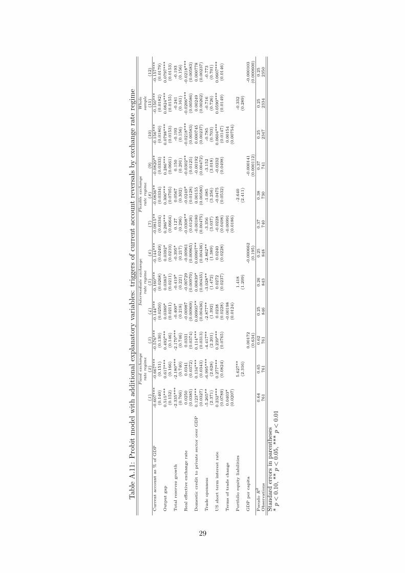
We begin by experimenting with the inclusion of additional control variables in our Probit

specification. In particular, we include variables measuring the change in the terms of trade,

portfolio equity liabilities and per capita GDP. As shown in Table A.11, the main results of the

analysis are robust to the inclusion of these additional controls. GDP per capita is insignificant

in all specifications we tried while the variables measuring the change in the terms of trade

and portfolio equity liabilities are significant only under fixed exchange rate regimes. Both an

improvement in the terms of trade an increase in portfolio equity liabilities are associated with

a higher likelihood of experiencing a reversal under fixed exchange rate regimes. Furthermore,

We include linear and quadratic time trends in the benchmark regressions in an effort to control

more effectively for the presence of possible time trends. As Table A.12 reports, the main results

of the trigger analysis are generally qualitatively robust to the specification changes.

We also test the robustness of our results to using an alternative measure of current account

reversals for the dependent variable. In particular, we define a current account correction as a

reversal if the current account deficit is larger than 2% of GDP when the reversal starts and

conditions 2, 3, and 4 (listed in Section 2) hold. While this stricter definition of a reversal

implies losing seven episodes of current account reversals, Table A.13 illustrates that our results

are qualitatively very similar to the benchmark analysis although the significance of some results

suffers from the reduction in the degrees of freedom.

We then proceed with the robustness analysis for the treatment effects model and begin

by including additional control variables in the benchmark specification. In particular, we add

net foreign direct investment, the old age dependency ratio and the labor force participation

rate as additional controls to the outcome equation (1) (Table A.14). In all of these additional

specifications, the reversal dummy remains insignificant, confirming our finding that there is

no causal link between reversals and growth in industrial economies. As regards the additional

controls, foreign direct investment does not turn out to be significant in any of the specifications

we tried. The old age dependency ratio, on the other hand, is always significant and its coefficient

is consistently negative. Intuitively, an increase in old age dependency leads to a higher burden

to social security and the public health system and implies that a smaller share of the population

is in productive employment. Moreover, older individuals tend to save less which reduces

national savings and investment. Finally, the labor force participation rate is positive and

significant under flexible exchange rates and in the whole sample but not under fixed exchange

rates. Indeed, higher labor force participation implies a higher supply of labor and this may

lead to a higher level of production and faster real GDP growth.

We also test the robustness of the treatment effects results to using a different definition of

current account reversals as previously done for the Probit model. Once again, our findings are

15

robust to this change in the definition of the dependent variable. Table A.15 shows that neither

the reversal dummy nor its lag are significant. Finally, we estimate the benchmark specification

of the outcome equation (1) using both a panel model with random effects and a panel model

with country fixed effects. The findings are reported in Tables A.16 and A.17 and support the

conclusions drawn on the benchmark model.

6 Conclusions

The present paper is motivated by the large current account imbalances experienced by advanced

economies both before the global crisis and presently and provides a systematic analysis of

current account reversals in these countries across different de-facto exchange rate regimes.

In particular, the paper examines whether industrial economies follow different patterns during

reversal episodes depending on the exchange rate regime they have in place. It identifies triggers

of reversals and examines the link between reversals and growth across different exchange rate

regimes.

The empirical analysis proceeds as follows: we initially identify 43 episodes of current account

reversals in 22 industrial economies between 1970 and 2007. The episodes are classified into

three groups of exchange rate regimes: fixed exchange rate regime, intermediate exchange rate

regime and flexible exchange rate regime. A brief event study sets the stage for the empirical

analysis which is split into two parts. In the first part, we estimate a Probit model for the

sample as a whole and separately for each group of exchange rate regime in an effort to identify

predictors of current account reversals. In the second part, we estimate a treatment effects

model to test whether reversals have an independent effect on growth and whether this effect

depends on the exchange rate regime in place.

We find that larger deficits and larger output gaps are associated with a higher probability

of experiencing reversals across all exchange rate regimes. Conversely, lower reserves growth,

higher domestic credit growth, higher US interest rates and a more closed economy raise the

probability of a reversal only under less flexible exchange rate regimes. A real exchange rate

depreciation, on the other hand, is a significant trigger only under more flexible regimes. Fur-

thermore, the treatment effects model suggests that adjustments of current account imbalances

are not per se harmful to economic activity, neither in the sample as a whole nor in the sub-

sample of fixed exchange rate regimes.

16

References

Algieri, B. and T. Bracke, “Patterns of Current Account Adjustment. Insight from Past Experience,” Open

Economies Review 22 (2011), 401–425.

Blanchard, O. and G. M. Milesi Ferretti, “Global Imbalances: In Midstream?,” CEPR Discussion Paper

7693, Centre for Economic Policy Research, 2010.

Bussiere, M. and M. Fratzscher, “Towards a New Early Warning System of Financial Crises,” Journal of

International Money and Finance 25 (2006), 953–973.

Chinn, M. and S.-J. Wei, “A Faith-based Initiative: Do We Really Know that a Flexible Exchange Rate Regime

Facilitates Current Account Adjustment?,” Review of Economics and Statistics 95 (2013), 168–184.

Croke, H., S. Kamin and S. Leduc, “An Assessment of the Disorderly Adjustment Hypothesis for Industrial

Economies,” International Finance 9 (2006), 37–61.

De Haan, L., H. Schokker and A. Tcherneva, “What Do Current Account Reversals in OECD Countries

Tell Us About the US Case?,” World Economy 31 (2008), 286–311.

Debelle, G. and G. Galati, “Current Account Adjustment and Capital Flows,” Review of International

Economics 15 (2007), 989–1013.

Edwards, S., “Financial Openness, Sudden Stops, and Current-Account Reversals,” American Economic Review

94 (2004a), 59–64.

———, “Thirty Years of Current Account Imbalances, Current Account Rever- sals, and Sudden Stops,” IMF

Staff Papers 51 (2004b), 1–49.

Feldstein, M., “Resolving the Global Imbalance: the Dollar and the U.S. Saving Rate,” Journal of Economic

Perspectives 22 (2008), 113–125.

Freund, C., “Current Account Adjustment in Industrialized Countries,” Journal of International Money and

Finance 24 (2005), 1278–1298.

Friedman, M., The Case for Flexible Exchange Rates. Essays in Positive Economics (Chicago: Chicago Uni-

versity Press, 1953).

Gosh, A., M. Terrones and J. Zettelmeyer, “Exchange Rate Regimes and External Adjustment: New

Answers to an Old Debate,” in C. Wyplosz, ed., The New International Monetary System: Essays in Honor

Of Alexander Swoboda (London: Routledge, 2010).

Heckman, J., “Dummy Endogenous Variables in a Simultaneous Equation System,” Econometrica 46 (1978),

931–960.

Ilzetzki, E., C. Reinhart and K. Rogoff, “Exchange Rate Arrangements Entering the 21st Century: Which

Anchor Will Hold?,” mimeo, 2008.

IMF, “World Economic Outlook,” (Washington, D.C.: International Monetary Fund, 2005).

———, “World Economic Outlook,” (Washington, D.C.: International Monetary Fund, 2006).

———, “Large External Imbalances in the Past: An Event Analysis,” in World Economic Outlook (Washington,

D.C.: International Monetary Fund, 2007).

17

———, “Pilot External Sector Report,” (Washington, D.C.: International Monetary Fund, 2012a).

———, “World Economic Outlook,” (Washington, D.C.: International Monetary Fund, 2012b).

Lane, P. and G. M. Milesi-Ferretti, “The external wealth of nations mark II: Revised and extended estimates

of foreign assets and liabilities, 19702004,” Journal of International Economics 73 (2007), 223–250.

———, “External Adjustment and the Global Crisis,” Journal of International Economics 88 (2012), 252–265.

Milesi-Ferretti, G. M. and A. Razin, “Sharp Reductions in Current Account Deficits. An Empirical Analy-

sis,” European Economic Review 42 (1998), 897–908.

———, “Current Account Reversals and Currency Crises: Empirical Regularities,” in P. Krugman, ed., Currency

Crises (Cambridge, MA: University of Chicago Press, 2000), 285–326.

Obstfeld, M., “Does the Current Account Still Matter?,” American Economic Review 102 (2012), 1–23.

Reinhart, C. and K. Rogoff, “The Modern History of Exchange Rate Arrangements: A Reinterpretation,”

Quarterly Journal of Economics 119 (2004), 1–48.

Serven, L. and H. Nguyen, “Global Imbalances Before and After the Global Crisis,” Policy Reserach Working

Paper 5354, World Bank, Washington, D.C., 2010.

18

Table A.1: Countries in sample

No. Country

1. Australia

2. Austria

3. Belgium

4. Canada

5. Denmark

6. Finland

7. France

8. Germany

9. Greece

10. Ireland

11. Italy

12. Korea

13. Japan

14. Netherlands

15. New Zealand

16. Norway

17. Portugal

18. Spain

19. Sweden

20. Switzerland

21. United Kingdom

22. United States

19

Tab

leA

.2:

Defi

nit

ion

san

dso

urc

esof

vari

able

s

Vari

ab

leN

am

eD

escr

ipti

onS

ourc

e

Cu

rren

tacc

ount

as%

ofG

DP

Cu

rren

tA

ccou

nt

as%

ofG

DP

OE

CD

,E

O

Dom

esti

ccr

edit

top

riva

tese

ctor

over

GD

PD

omes

tic

cred

itto

pri

vate

sect

oras

%of

GD

PW

B,

WD

I

Dom

esti

cd

emand

Tot

ald

omes

tic

dem

and

OE

CD

,E

O

Nom

inal

GD

PG

ross

dom

esti

cp

rod

uct

OE

CD

,E

O

Ou

tpu

tga

pO

utp

ut

gap

in%

ofp

oten

tial

outp

ut

OE

CD

,E

Oan

dIM

F,

WE

O

Rea

leff

ecti

veex

chan

gera

teR

eal

effec

tive

exch

ange

rate

(27

cty)i

nd

ex(2

000=

100)

,C

PI

bas

edB

IS

Rea

lG

DP

Gro

ssd

omes

tic

pro

du

ctO

EC

D,

EO

Gov

ern

men

tb

ud

get

bala

nce

as%

of

GD

PG

over

nm

ent

pri

mar

yb

alan

ceas

%of

GD

PO

EC

D,

EO

Gov

ern

men

tco

nsu

mp

tion

Gov

ern

men

tco

nsu

mp

tion

exp

end

itu

reIM

F,

IFS

Inve

stm

ent

Gro

ssto

tal

fixed

cap

ital

OE

CD

,E

O

Tot

al

fore

ign

rese

rves

Tot

alre

serv

esm

inu

sgo

ldW

B,

WD

I

Sh

ort

term

inte

rest

rate

Mon

eym

arke

tra

teIM

F,

IFS

Con

sum

erp

rice

ind

exC

onsu

mpti

onp

rice

ind

ex(2

000=

100)

OE

CD

,E

O

De-

fact

oex

chan

ge

rate

regim

eF

ine

exch

ange

rate

regi

me

clas

sifi

cati

onIl

zetz

ki

etal

.(2

008)

Tra

de

op

enn

ess

Exp

orts

plu

sIm

por

tsas

%of

GD

PW

B,

WD

I

Ter

ms

of

trad

eT

erm

sof

trad

eW

B,

WD

I

Infl

atio

nra

teC

onsu

mp

tion

pri

cein

dex

(200

0=10

0)gr

owth

OE

CD

,E

O

For

eign

dir

ect

inves

tmen

tas

%of

GD

PF

orei

gnd

irec

tin

ves

tmen

tas

%of

GD

PL

ane

and

Miles

i-F

erre

tti

(200

7)

Old

age

dep

end

ency

rati

oO

ldag

ed

epen

den

cyra

tio

as%

ofw

orkin

gag

ep

opu

lati

onW

B,

WD

I

Lab

or

forc

ep

art

icip

ati

on

rate

Lab

orfo

rce

par

tici

pat

ion

rate

as%

ofw

orkin

gag

ep

opu

lati

onO

EC

D,

EO

GD

Pp

erca

pit

aG

DP

per

cap

ita

WB

,W

DI

Port

foli

oeq

uit

yli

abil

itie

sP

ortf

olio

equ

ity

liab

ilit

ies

Lan

ean

dM

iles

i-F

erre

tti

(200

7)

20

Figure A.2: Current account reversals by country between 1970 and 2007

−6

−4

−2

02

1970q1 1980q1 1990q1 2000q1Time

Australia−

6−

4−

20

24

1970q1 1980q1 1990q1 2000q1Time

Austria

−1

0−

50

51

0

1970q1 1980q1 1990q1 2000q1Time

Belgium

−6

−4

−2

02

4

1970q1 1980q1 1990q1 2000q1Time

Canada

−6

−4

−2

02

4

1970q1 1980q1 1990q1 2000q1Time

Denmark

−1

0−

50

51

0

1970q1 1980q1 1990q1 2000q1Time

Finland

−2

02

4

1970q1 1980q1 1990q1 2000q1Time

France

−2

02

46

8

1970q1 1980q1 1990q1 2000q1Time

Germany

−1

5−

10

−5

05

1970q1 1980q1 1990q1 2000q1Time

Greece

−1

5−

10

−5

05

1970q1 1980q1 1990q1 2000q1Time

Ireland

−6

−4

−2

02

4

1970q1 1980q1 1990q1 2000q1Time

Italy

−2

02

46

1970q1 1980q1 1990q1 2000q1Time

Japan

Current account as % of GDP Time of the reversal

21

Figure A.3: Current account reversals by country between 1970 and 2007

−2

0−

10

01

02

0

1970q1 1980q1 1990q1 2000q1Time

Korea−

50

51

0

1970q1 1980q1 1990q1 2000q1Time

Netherlands

−1

5−

10

−5

05

1970q1 1980q1 1990q1 2000q1Time

New Zealand

−2

0−

10

01

02

0

1970q1 1980q1 1990q1 2000q1Time

Norway

−2

0−

15

−1

0−

50

5

1970q1 1980q1 1990q1 2000q1Time

Portugal

−2

0−

10

01

0

1970q1 1980q1 1990q1 2000q1Time

Spain

−5

05

10

1970q1 1980q1 1990q1 2000q1Time

Sweden

05

10

15

20

1970q1 1980q1 1990q1 2000q1Time

Switzerland

−6

−4

−2

02

4

1970q1 1980q1 1990q1 2000q1Time

United Kingdom

−6

−4

−2

02

1970q1 1980q1 1990q1 2000q1Time

United States

Current account as % of GDP Time of the reversal

22

Table A.3: The natural classification bucket, the Reinhart-Rogoff (RR)(2004) fine grid

Natural classification bucket RR Fine grid

No separate legal tender 1

Preannounced peg or currency board arrangement 2

Preannounced horizontal band that is narrower than or equal to +/-2% 3

De facto peg 4

Preannounced crawling peg 5

Preannounced crawling band that is narrower than or equal to +/-2% 6

De facto crawling peg 7

De facto crawling band that is narrower than or equal to +/-2% 8

Preannounced crawling band that is wider than +/-2% 9

De facto crawling band that is narrower than or equal to +/-5% 10

Noncrawling band that is narrower than or equal to +/-2% 11

Managed floating 12

Freely floating 13

Freely falling 14

Table A.4: Exchange rate regime classification

Our own classification RR’s fine grid codes

Fixed exchange rate regime 1, 2, 3, 4

Intermediate exchange rate regime 5, 6, 7, 8, 9, 10, 11

Flexible exchange rate regime 12, 13

Table A.5: Exchange rate regimes in industrial countries,1970-2007

Exchange rate 1970q1-1979q4 1980q1-1989q4 1990q1-1999q4 2000q1-2007q4 1970q1-2007q4

regime Obs. % Obs. % Obs. % Obs. % Obs. %

Fixed 264 30 119 13.52 310 35.23 384 54.55 1077 32.21

Intermediate 446 50.68 481 54.66 266 30.23 124 17.61 1317 39.38

Flexible 170 19.32 280 31.82 298 33.86 196 27.84 944 28.23

Total 880 100.0 880 100.0 880 100.0 704 100.0 3344 100.0

23

Table A.6: Episodes of current account reversals by exchange rate regimeNo. Country Year Current Account Exchange rate regime

as % of GDP

1. Australia 1989q2 -6.17 Flexible

2. Australia 1999q2 -5.87 Flexible

3. Austria 1980q2 -6.02 Intermediate

4. Austria 1997q4 -3.06 Fixed

5. Austria 2001q1 -2.12 Fixed

6. Belgium 1982q1 -7.53 Fixed

7. Canada 1981q3 -4.67 Intermediate

8. Canada 1993q4 -4.23 Intermediate

9. Canada 1997q3 -2.47 Intermediate

10. Denmark 1986q2 -6.18 Intermediate

11. Denmark 1998q4 -2.45 Intermediate

12. Finland 1991q1 -6.33 Intermediate

13. France 1976q3 -2.33 Intermediate

14. France 1982q3 -1.16 Intermediate

15. France 1990q3 -0.84 Fixed

16. Germany 1980q4 -2.45 Flexible

17. Germany 2000q3 -2.30 Fixed

18. Greece 1985q3 -8.57 Flexible

19. Greece 1990q1 -6.06 Intermediate

20. Ireland 1982q1 -14.90 Intermediate

21. Ireland 1990q4 -3.84 Intermediate

22. Italy 1974q3 -5.06 Intermediate

23. Italy 1981q1 -4.01 Flexible

24. Italy 1992q3 -2.72 Intermediate

25. Japan 1974q1 -2.29 Intermediate

26. Japan 1979q4 -1.79 Flexible

27. Korea 1980q1 -9.66 Fixed

28. Korea 1996q3 -5.02 Intermediate

29. The Netherlands 1980q1 -1.31 Intermediate

30. The Netherlands 2000q3 -1.22 Fixed

31. New Zealand 1984q4 -15.12 Intermediate

32. New Zealand 1999q4 -8.44 Flexible

33. Norway 1986q2 -11.51 Flexible

34. Norway 1998q4 -3.57 Flexible

35. Portugal 1981q4 -17.43 Intermediate

36. Spain 1982q2 -18.32 Intermediate

37. Sweden 1982q4 -4.89 Intermediate

38. Sweden 1992q1 -3.34 Intermediate

39. Switzerland 1980q4 -1.08 Flexible

40. United Kingdom 1974q2 -5.56 Flexible

41. United Kingdom 1979q1 -4.31 Flexible

42. United Kingdom 1988q4 -1.45 Flexible

43. United States 1987q4 -3.38 Flexible

24

Figure A.4: De-facto exchange rate regime by country between 1970 and 2007 according to thedata provided by Ilzetzki, Reinhart and Rogoff (2008)

05

10

15

1970q1 1980q1 1990q1 2000q1Time

Australia0

24

68

1970q1 1980q1 1990q1 2000q1Time

Austria

12

34

1970q1 1980q1 1990q1 2000q1Time

Belgium

24

68

10

1970q1 1980q1 1990q1 2000q1Time

Canada

24

68

1970q1 1980q1 1990q1 2000q1Time

Denmark

05

10

15

1970q1 1980q1 1990q1 2000q1Time

Finland

05

10

15

1970q1 1980q1 1990q1 2000q1Time

France

05

10

15

1970q1 1980q1 1990q1 2000q1Time

Germany

05

10

15

1970q1 1980q1 1990q1 2000q1Time

Greece

02

46

8

1970q1 1980q1 1990q1 2000q1Time

Ireland

05

10

15

1970q1 1980q1 1990q1 2000q1Time

Italy

05

10

15

1970q1 1980q1 1990q1 2000q1Time

Japan

Exchange rate regime

25

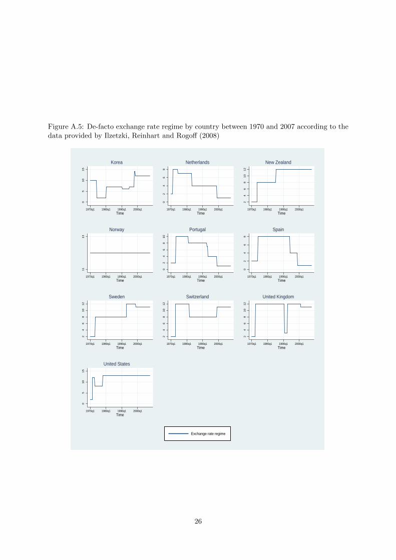
Figure A.5: De-facto exchange rate regime by country between 1970 and 2007 according to thedata provided by Ilzetzki, Reinhart and Rogoff (2008)

05

10

15

1970q1 1980q1 1990q1 2000q1Time

Korea0

24

68

1970q1 1980q1 1990q1 2000q1Time

Netherlands

24

68

10

12

1970q1 1980q1 1990q1 2000q1Time

New Zealand

11

13

1970q1 1980q1 1990q1 2000q1Time

Norway

02

46

81

0

1970q1 1980q1 1990q1 2000q1Time

Portugal

02

46

8

1970q1 1980q1 1990q1 2000q1Time

Spain

24

68

10

12

1970q1 1980q1 1990q1 2000q1Time

Sweden

24

68

10

12

1970q1 1980q1 1990q1 2000q1Time

Switzerland

24

68

10

12

1970q1 1980q1 1990q1 2000q1Time

United Kingdom

05

10

15

1970q1 1980q1 1990q1 2000q1Time

United States

Exchange rate regime

26

Table A.7: Average dynamics of the current account as % of GDP around the adjustmentepisode by exchange rate regime

Year relative to deficit minimum

-3 -2 -1 0 1 2 3

Fixed exchange rate -0.47 -1.08 -1.82 -3.82 -1.49 -0.05 0.74

Intermediate exchange rate -1.71 -2.13 -3.31 -6.19 -2.85 -0.67 0.30

Flexible exchange rate 0.02 -0.12 -2.05 -4.87 -2.16 -0.09 0.37

Table A.8: Average dynamics of the real GDP growth around the adjustment episode by ex-change rate regime

Year relative to deficit minimum

-3 -2 -1 0 1 2 3

Fixed exchange rate 4.04 4.13 3.32 2.12 1.27 2.20 2.02

Intermediate exchange rate 3.16 3.02 3.51 3.06 1.05 1.43 2.19

Flexible exchange rate 2.82 3.94 3.83 3.05 2.51 0.46 1.76

27

Table A.9: Average dynamics of the real domestic demand growth around the adjustmentepisode by exchange rate regime

Year relative to deficit minimum

-3 -2 -1 0 1 2 3

Fixed exchange rate 4.09 4.69 3.64 2.19 0.80 0.66 1.54

Intermediate exchange rate 3.31 3.22 2.99 3.05 1.33 -0.57 0.64

Flexible exchange rate 2.81 3.70 4.63 4.55 2.27 0.27 1.00

Table A.10: Average dynamics of the real effective exchange rate index around the adjustmentepisode by exchange rate regime

Year relative to deficit minimum

-3 -2 -1 0 1 2 3

Fixed exchange rate 115.07 112.90 110.80 108.20 107.03 108.88 110.83

Intermediate exchange rate 111.70 111.78 111.08 109.42 107.49 103.15 103.74

Flexible exchange rate 103.97 101.45 99.60 96.84 95.76 97.77 97.86

28

Tab

leA

.11:

Pro

bit

mod

elw

ith

add

itio

nal

exp

lan

ator

yva

riab

les:

trig

gers

ofcu

rren

tac

cou

nt

reve

rsal

sby

exch

ange

rate

regi

me

Fixed

exchange

Intermed

iate

exchange

Flexible

exchange

Whole

rate

regim

era

teregim

era

teregim

esa

mple

(1)

(2)

(3)

(4)

(5)

(6)

(7)

(8)

(9)

(10)

(11)

(12)

Curr

ent

account

as

%of

GD

P-0

.607***

-0.6

67***

-0.5

76***

-0.1

44***

-0.1

60***

-0.1

44***

-0.0

815**

-0.0

836**

-0.0

820**

-0.1

56***

-0.1

50***

-0.1

57***

(0.1

40)

(0.1

51)

(0.1

30)

(0.0

250)

(0.0

268)

(0.0

249)

(0.0

334)

(0.0

334)

(0.0

333)

(0.0

180)

(0.0

182)

(0.0

179)

Outp

ut

gap

0.5

15***

0.6

17***

0.4

92***

0.0

389*

0.0

383*

0.0

392*

0.2

86***

0.3

06***

0.2

86***

0.0

798***

0.0

824***

0.0

797***

(0.1

52)

(0.1

66)

(0.1

46)

(0.0

211)

(0.0

211)

(0.0

210)

(0.0

664)

(0.0

705)

(0.0

661)

(0.0

153)

(0.0

155)

(0.0

153)

Tota

lre

serv

es

gro

wth

-2.3

35***

-2.1

80***

-2.1

70***

-0.4

00*

-0.4

19*

-0.3

95*

0.1

27

0.0

567

0.1

50

-0.1

93

-0.2

41

-0.1

93

(0.7

66)

(0.7

40)

(0.7

46)

(0.2

18)

(0.2

21)

(0.2

17)

(0.2

96)

(0.3

02)

(0.2

91)

(0.1

56)

(0.1

61)

(0.1

56)

Real

eff

ecti

ve

exchange

rate

0.0

250

0.0

341

0.0

331

-0.0

0987

-0.0

0729

-0.0

0961

-0.0

308**

-0.0

249*

-0.0

302**

-0.0

218***

-0.0

206***

-0.0

218***

(0.0

385)

(0.0

372)

(0.0

374)

(0.0

0969)

(0.0

0970)

(0.0

0965)

(0.0

126)

(0.0

128)

(0.0

125)

(0.0

0583)

(0.0

0586)

(0.0

0583)

Dom

est

iccre

dit

topri

vate

secto

rover

GD

P0.1

23***

0.1

34***

0.1

14***

0.0

0905**

0.0

0839*

0.0

0907**

-0.0

0180

0.0

0155

-0.0

0192

0.0

00745

0.0

0249

0.0

00778

(0.0

327)

(0.0

343)

(0.0

313)

(0.0

0436)

(0.0

0435)

(0.0

0436)

(0.0

0475)

(0.0

0580)

(0.0

0472)

(0.0

0237)

(0.0

0262)

(0.0

0237)

Tra

de

op

enness

-5.2

65**

-6.9

95***

-4.4

17**

-2.8

77**

-3.0

28**

-2.8

62**

-3.3

56

-1.0

85

-3.1

52

-0.7

85

-0.7

16

-0.7

73

(2.3

71)

(2.6

28)

(2.2

01)

(1.3

92)

(1.4

72)

(1.3

89)

(3.0

37)

(3.2

56)

(3.0

18)

(0.7

03)

(0.7

26)

(0.7

01)

US

short

term

inte

rest

rate

0.2

32***

0.2

77***

0.2

39***

0.0

238

0.0

272

0.0

240

-0.0

228

-0.0

475

-0.0

232

0.0

604***

0.0

590***

0.0

607***

(0.0

789)

(0.0

824)

(0.0

765)

(0.0

228)

(0.0

237)

(0.0

228)

(0.0

498)

(0.0

532)

(0.0

498)

(0.0

147)

(0.0

149)

(0.0

146)

Term

sof

trade

change

0.0

403*

-0.0

0198

-0.0

0991

0.0

0154

(0.0

207)

(0.0

124)

(0.0

186)

(0.0

0754)

Port

folio

equit

yliabilit

ies

5.6

27**

1.4

18

-2.6

40

-0.3

32

(2.3

16)

(1.2

09)

(2.4

11)

(0.2

89)

GD

Pp

er

capit

a0.0

0172

-0.0

00662

-0.0

00141

-0.0

00103

(0.6

34)

(0.1

95)

(0.0

00112)

(0.0

00600)

Pse

udoR

20.6

40.6

50.6

20.2

50.2

60.2

50.3

70.3

80.3

70.2

50.2

50.2

5O

bse

rvati

ons

761

761

761

846

843

848

740

730

741

2347

2334

2350

Sta

ndard

erro

rsin

pare

nth

eses

*p<

0.1

0,

**p<

0.0

5,

***p<

0.0

1

29

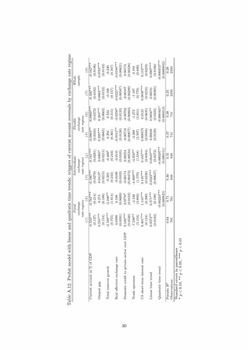
Tab

leA

.12:

Pro

bit

mod

elw

ith

lin

ear

an

dqu

adra

tic

tim

etr

end

s:tr

igge

rsof

curr

ent

acco

unt

reve

rsal

sby

exch

ange

rate

regi

me

Fixed

Interm

ediate

Flexible

Whole

exch

ange

exch

ange

exch

ange

sample

rate

regime

rate

regime

rate

regime

(1)

(2)

(3)

(4)

(5)

(6)

(7)

(8)

Cu

rren

tacc

ou

nt

as

%of

GD

P-0

.559***

-0.7

62***

-0.1

86***

-0.1

81***

-0.0

864**

-0.0

969***

-0.1

60***

-0.1

82***

(0.1

37)

(0.2

14)

(0.0

279)

(0.0

281)

(0.0

343)

(0.0

372)

(0.0

182)

(0.0

196)

Ou

tpu

tgap

0.5

55***

0.2

73

0.0

419*

0.0

365*

0.2

89***

0.2

93***

0.0

802***

0.0

783***

(0.1

54)

(0.1

88)

(0.0

215)

(0.0

215)

(0.0

665)

(0.0

663)

(0.0

152)

(0.0

143)

Tota

lre

serv

esgro

wth

-2.1

69***

-2.1

06**

-0.3

83

-0.4

60*

0.2

04

0.3

34

-0.1

68

-0.2

30

(0.7

55)

(1.0

14)

(0.2

33)

(0.2

43)

(0.3

01)

(0.3

15)

(0.1

57)

(0.1

67)

Rea

leff

ecti

ve

exch

an

ge

rate

0.0

399

0.1

08

-0.0

109

-0.0

141

-0.0

315**

-0.0

250*

-0.0

225***

-0.0

194***

(0.0

391)

(0.0

689)

(0.0

103)

(0.0

105)

(0.0

126)

(0.0

133)

(0.0

0587)

(0.0

0621)

Dom

esti

ccr

edit

top

rivate

sect

or

over

GD

P0.1

00***

0.0

778*

-0.0

0174

0.0

0254

-0.0

0716

-0.0

0762

-0.0

0187

0.0

0174

(0.0

330)

(0.0

410)

(0.0

0473)

(0.0

0534)

(0.0

0877)

(0.0

0903)

(0.0

0299)

(0.0

0338)

Tra

de

op

enn

ess

-7.5

98**

-4.5

38

-4.8

69***

-4.0

59**

-4.3

68

-1.2

72

-1.1

87

0.1

94

(3.1

53)

(3.6

92)

(1.5

79)

(1.6

18)

(3.5

07)

(3.8

51)

(0.7

70)

(0.8

30)

US

short

term

inte

rest

rate

0.4

01***

1.1

44***

0.1

45***

0.1

83***

0.0

00575

0.0

123

0.0

838***

0.1

53***

(0.1

24)

(0.3

90)

(0.0

338)

(0.0

394)

(0.0

594)

(0.0

635)

(0.0

216)

(0.0

259)

Lin

ear

tim

etr

end

0.0

372**

0.5

71***

0.0

322***

0.0

843***

0.0

0848

0.0

856**

0.0

0531

0.0

907***

(0.0

182)

(0.1

98)

(0.0

0647)

(0.0

272)

(0.0

120)

(0.0

424)

(0.0

0365)

(0.0

160)

Qu

ad

rati

cti

me

tren

d-0

.00233***

-0.0

00297**

-0.0

00401*

-0.0

00453***

(0.0

00825)

(0.0

00151)

(0.0

00213)

(0.0

000832)

Pse

ud

oR

20.6

40.7

10.3

00.3

10.3

70.3

80.2

50.2

8O

bse

rvati

on

s761

761

848

848

741

741

2350

2350

Sta

ndard

erro

rsin

pare

nth

eses

*p<

0.1

0,

**p<

0.0

5,

***p<

0.0

1

30

Table A.13: Probit model: triggers of current account reversals by exchange rate regimeFixed Intermediate Flexible Whole

exchange exchange exchange samplerate regime rate regime rate regime

(1 ) (2 ) (3 ) (4 )Current account as % of GDP -0.641*** -0.144*** -0.0699** -0.146***

(0.166) (0.0249) (0.0327) (0.0181)

Output gap 0.275 0.0392* 0.298*** 0.0702***(0.180) (0.0210) (0.0673) (0.0146)

Total reserves growth -1.047 -0.395* 0.122 -0.151(0.893) (0.217) (0.294) (0.155)

Real effective exchange rate 0.0217 -0.00962 -0.0365*** -0.0224***(0.0471) (0.00965) (0.0131) (0.00594)

Domestic credit to private sector over GDP 0.127*** 0.00907** -0.000213 0.000668(0.0412) (0.00436) (0.00482) (0.00244)

Trade openness -3.695** -2.863** -4.844 -1.624**(1.830) (1.389) (3.122) (0.806)

US short term interest rate 0.195* 0.0240 0.00725 0.0633***(0.109) (0.0228) (0.0509) (0.0153)

Pseudo R2 0.65 0.25 0.36 0.26Observations 761 848 741 2350

Standard errors in parentheses.* p < 0.10, ** p < 0.05, *** p < 0.01The dependent variable is equal to 1 only if the current account is lower than 2% of GDP.

31

Tab

leA

.14:

Tre

atm

ent

effec

tsm

od

elw

ith

add

itio

nal

regr

esso

rs:

curr

ent

acco

unt

rever

sals

’eff

ect

onre

alec

onom

icp

erfo

rman

ceFixed

exch

ange

Interm

ediate

exch

ange

Flexibleexch

ange

Whole

rate

regime

rate

regime

rate

regime

sample

(1)

(2)

(3)

(4)

(5)

(6)

(7)

(8)

(9)

(10)

(11)

(12)

Rea

lG

DP

gro

wth

Inves

tmen

tas

%of

GD

P18.3

7***

22.2

0***

17.7

9***

28.5

8***

30.3

6***

24.7

1***

30.0

3***

29.6

3***

24.6

8***

27.9

2***

28.6

7***

24.5

4***

(3.3

92)

(3.3

56)

(3.3

91)

(2.2

43)

(2.4

10)

(2.5

80)

(2.6

26)

(2.5

89)

(2.5

86)

(1.3

01)

(1.3

02)

(1.3

75)

Tra

de

op

enn

ess

0.7

88*

2.7

35***

1.2

30***

10.7

2***

12.0

3***

10.6

8***

7.4

79***

8.2

15***

4.4

36***

4.5

78***

5.4

82***

4.5

77***

(0.4

65)

(0.5

17)

(0.4

30)

(0.9

98)

(1.0

34)

(0.9

64)

(1.6

31)

(1.6

35)

(1.6

19)

(0.4

58)

(0.4

66)

(0.4

26)

Gover

nm

ent

con

sum

pti

on

-37.1

5***

-32.2

6***

-40.5

7***

-40.3

2***

-31.3

1***

-39.4

2***

-27.0

2***

-20.4

8***

-15.7

1***

-25.2

8***

-16.4

1***

-21.6

5***

exp

end

itu

reas

%of

GD

P(6

.398)

(6.1

54)

(6.1

85)

(3.8

10)

(5.2

98)

(4.4

40)

(3.4

14)

(4.8

59)

(3.5

28)

(1.8

30)

(2.6

26)

(1.8

94)

Infl

ati

on

rate

-0.2

62***

-0.3

35***

-0.2

75***

-0.2

09***

-0.2

37***

-0.1

87***

-0.3

23***

-0.3

38***

-0.3

26***

-0.1

99***

-0.2

25***

-0.1

80***

(0.0

261)

(0.0

285)

(0.0

262)

(0.0

183)

(0.0

201)

(0.0

203)

(0.0

271)

(0.0

272)

(0.0

285)

(0.0

108)

(0.0

121)

(0.0

119)

Ter

ms

of

trad

ech

an

ge

0.0

207

0.0

0687

0.0

246

0.0

428

0.0

381

0.0

397

-0.0

143

-0.0

148

-0.0

0167

0.0

228

0.0

178

0.0

285

(0.0

508)

(0.0

498)

(0.0

508)

(0.0

328)

(0.0

326)

(0.0

341)

(0.0

279)

(0.0

277)

(0.0

268)

(0.0

203)

(0.0

202)

(0.0

206)

Rev

ersa

l1.4

08

0.2

00

0.9

29

-0.9

41

-0.8

36

-0.1

33

-1.1

26

-0.4

35

-1.7

66

1.3

37

1.8

04

1.9

29

(2.2

13)

(2.1

81)

(2.1

33)

(2.2

89)

(2.2

88)

(2.2

61)

(2.0

90)

(1.9

59)

(1.7

35)

(1.3

26)

(1.2

89)

(1.4

58)

Fore

ign

dir

ect

inves

tmen

t0.0

102

0.0

235

0.0

136

-0.0

0176

as

%of

GD

P(0

.00739)

(0.0

355)

(0.0

555)

(0.0

0861)

Old

age

dep

end

ency

rati

o-0

.300***

-0.1

54**

-0.0

709*

-0.1

15***

(0.0

533)

(0.0

685)

(0.0

374)

(0.0

252)

Lab

or

forc

ep

art

icip

ati

on

rate

-0.0

469

0.1

04

0.7

98***

0.2

20***

(0.0

539)

(0.0

709)

(0.0

966)

(0.0

421)

Rev

ersa

lL

.Cu

rren

tacc

ou

nt

-0.3

01*

-0.3

01*

-0.3

03*

-0.0

648*

-0.0

648*

-0.0

626*

-0.0

977

-0.1

02

-0.0

875

-0.0

934***

-0.1

00***

-0.0

899***

as

%of

GD

P(0

.164)

(0.1

64)

(0.1

66)

(0.0

354)

(0.0

354)

(0.0

359)

(0.0

625)

(0.0

643)

(0.0

616)

(0.0

263)

(0.0

262)

(0.0

268)

L.O

utp

ut

gap

0.3

41

0.3

41

0.3

90*

0.0

359

0.0

359

0.0

376

0.2

57*

0.2

65*

0.3

29**

0.0

491***

0.0

483***

0.0

516**

(0.2

10)

(0.2

10)

(0.2

30)

(0.0

346)

(0.0

346)

(0.0

351)

(0.1

40)

(0.1

46)

(0.1

32)

(0.0

169)

(0.0

169)

(0.0

216)

L.T

ota

lre

serv

esgro

wth

-1.2

98

-1.2

98

-1.3

06

-0.5

04

-0.5

04

-0.5

65

-0.1

21

-0.1

08

-0.1

49

-0.3

10

-0.3

28

-0.3

21

(1.2

35)

(1.2

35)

(1.2

85)

(0.3

88)

(0.3

88)

(0.4

01)

(0.5

58)

(0.5

46)

(0.5

75)

(0.2

75)

(0.2

76)

(0.2

80)

L.R

eal

effec

tive

exch

ange

0.0

0784

0.0

0784

0.0

275

-0.0

166**

-0.0

166**

-0.0

160*

-0.0

173

-0.0

123

-0.0

210*

-0.0

216***

-0.0

211***

-0.0

214***

rate

(0.0

596)

(0.0

596)

(0.0

728)

(0.0

0817)

(0.0

0817)

(0.0

0829)

(0.0

111)

(0.0

110)

(0.0

121)

(0.0

0398)

(0.0

0397)

(0.0

0399)

L.T

rad

eop

enn

ess

-2.3

60

-2.3

60

-2.0

40

-3.5

94*

-3.5

94*

-3.4

75*

-4.4

78

-4.8

87

-3.8

74

-1.2

81

-1.1

99

-1.2

13

(2.9

50)

(2.9

50)

(3.0

97)

(1.8

52)

(1.8

52)

(1.8

74)

(3.9

97)

(4.1

31)

(4.0

80)

(0.9

70)

(0.9

71)

(0.9

74)

L.D

om

esti

ccr

edit

to0.0

651

0.0

651

0.0

591

0.0

0921

0.0

0921

0.0

0858

0.0

0505

0.0

0292

0.0

0591

0.0

0249

0.0

0141

0.0

0207

pri

vate

sect

or

over

GD

P(0

.0429)

(0.0

429)

(0.0

451)

(0.0

0693)

(0.0

0693)

(0.0

0706)

(0.0

0839)

(0.0

0828)

(0.0

0866)

(0.0

0393)

(0.0

0397)

(0.0

0395)

L.U

Sin

tere

stra

te0.1

42

0.1

42

0.1

47

0.0

281

0.0

281

0.0

320

0.0

313

-0.0

271

0.0

495

0.0

452*

0.0

399*

0.0

481**

(0.1

23)

(0.1

23)

(0.1

33)

(0.0

362)

(0.0

362)

(0.0

359)

(0.0

895)

(0.0

863)

(0.0

997)

(0.0

233)

(0.0

232)

(0.0

236)

Lam

bd

a-0

.530

-0.0

398

-0.2

80

0.4

58

0.4

16

0.0

991

0.6

11

0.2

66

0.9

64

-0.4

68

-0.6

65

-0.6

82

(1.1

00)

(1.0

86)

(1.0

76)

(1.0

10)

(1.0

10)

(1.0

08)

(0.9

84)

(0.9

38)

(0.8

04)

(0.5

72)

(0.5

55)

(0.6

21)

Waldχ

23052.1

***

3224.2

***

3096.3

***

2873.7

***

2882.1

***

2832.8

***

1918.0

***

1974.5

***

2106.6

***

6255.8

***

6325.7

9***

6237.9

***

Ob

serv

ati

on

s755

759

754

829

834

796

727

733

710

2311

2326

2260

Sta

ndard

erro

rsin

pare

nth

eses

*p<

0.1

0,

**p<

0.0

5,

***p<

0.0

1

32

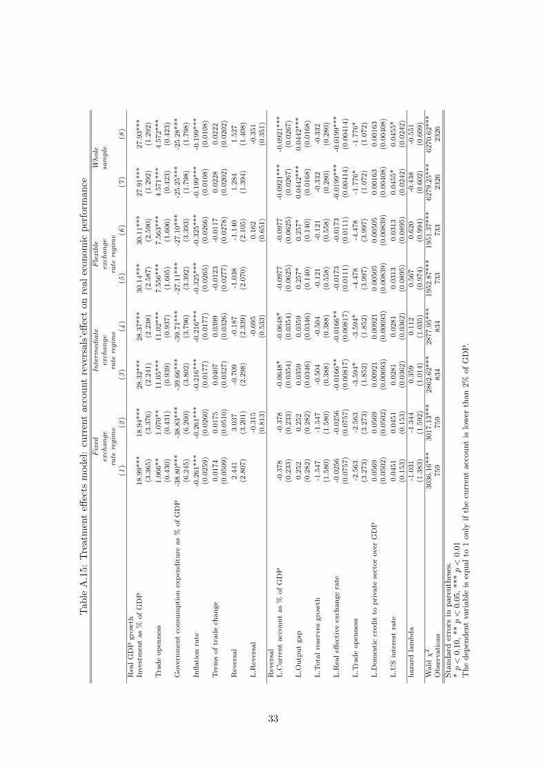
Tab

leA

.15:

Tre

atm

ent

effec

tsm

od

el:

curr

ent

acco

unt

rever

sals

’eff

ect

onre

alec

onom

icp

erfo

rman

ceFixed

Interm

ediate

Flexible

Whole

exch

ange

exch

ange

exch

ange

sample

rate

regime

rate

regime

rate

regime

(1)

(2)

(3)

(4)

(5)

(6)

(7)

(8)

Rea

lG

DP

gro

wth

Inves

tmen

tas

%of

GD

P18.9

9***

18.9

4***

28.3

2***

28.3

7***

30.1

4***

30.1

1***

27.9

1***

27.9

3***

(3.3

65)

(3.3

76)

(2.2

41)

(2.2

38)

(2.5

87)

(2.5

90)

(1.2

92)

(1.2

92)

Tra

de

op

enn

ess

1.0

66**

1.0

70**

11.0

5***

11.0

2***

7.5

56***

7.5

63***

4.5

71***

4.5

72***

(0.4

30)

(0.4

31)

(0.9

39)

(0.9

37)

(1.6

05)

(1.6

06)

(0.4

23)

(0.4

23)

Gover

nm

ent

con

sum

pti

on

exp

end

itu

reas

%of

GD

P-3

8.8

0***

-38.8

3***

-39.6

6***

-39.7

1***

-27.1

1***

-27.1

0***

-25.2

5***

-25.2

8***

(6.2

45)

(6.2

60)

(3.8

02)

(3.7

96)

(3.3

92)

(3.3

93)

(1.7

98)

(1.7

98)

Infl

ati

on

rate

-0.2

61***

-0.2

61***

-0.2

16***

-0.2

16***

-0.3

25***

-0.3

25***

-0.1

99***

-0.1

99***

(0.0

259)

(0.0

260)

(0.0

177)

(0.0

177)

(0.0

265)

(0.0

266)

(0.0

108)

(0.0

108)

Ter

ms

of

trad

ech

an

ge

0.0

174

0.0

175

0.0

407

0.0

399

-0.0

123

-0.0

117

0.0

228

0.0

222

(0.0

509)

(0.0

510)

(0.0

327)

(0.0

326)

(0.0

277)

(0.0

278)

(0.0

202)

(0.0

202)

Rev

ersa

l2.4

41

3.0

37

-0.7

09

-0.1

87

-1.0

38

-1.1

40

1.2

84

1.5

27

(2.8

07)

(3.2

01)

(2.2

98)

(2.3

39)

(2.0

70)

(2.1

05)

(1.3

94)

(1.4

08)

L.R

ever

sal

-0.3

15

-0.6

95

0.1

62

-0.3

51

(0.8

13)

(0.5

33)

(0.6

51)

(0.3

51)

Rev

ersa

lL

.Cu

rren

tacc

ou

nt

as

%of

GD

P-0

.378

-0.3

78

-0.0

648*

-0.0

648*

-0.0

977

-0.0

977

-0.0

921***

-0.0

921***

(0.2

33)

(0.2

33)

(0.0

354)

(0.0

354)

(0.0

625)

(0.0

625)

(0.0

267)

(0.0

267)

L.O

utp

ut

gap

0.2

52

0.2

52

0.0

359

0.0

359

0.2

57*

0.2

57*

0.0

442***

0.0

442***

(0.2

82)

(0.2

82)

(0.0

346)

(0.0

346)

(0.1

40)

(0.1

40)

(0.0

168)

(0.0

168)

L.T

ota

lre

serv

esgro

wth

-1.5

47

-1.5

47

-0.5

04

-0.5

04

-0.1

21

-0.1

21

-0.3

32

-0.3

32

(1.5

80)

(1.5

80)

(0.3

88)

(0.3

88)

(0.5

58)

(0.5

58)

(0.2

80)

(0.2

80)

L.R

eal

effec

tive

exch

an

ge

rate

-0.0

256

-0.0

256

-0.0

166**

-0.0

166**

-0.0

173

-0.0

173

-0.0

199***

-0.0

199***

(0.0

757)

(0.0

757)

(0.0

0817)

(0.0

0817)

(0.0

111)

(0.0

111)

(0.0

0414)

(0.0

0414)

L.T

rad

eop

enn

ess

-2.5

63

-2.5

63

-3.5

94*

-3.5

94*

-4.4

78

-4.4

78

-1.7

76*

-1.7

76*

(3.2

73)

(3.2

73)

(1.8

52)

(1.8

52)

(3.9

97)

(3.9

97)

(1.0

72)

(1.0

72)

L.D

om

esti

ccr

edit

top

rivate

sect

or

over

GD

P0.0

569

0.0

569

0.0

0921

0.0

0921

0.0

0505

0.0

0505

0.0

0163

0.0

0163

(0.0

502)

(0.0

502)

(0.0

0693)

(0.0

0693)

(0.0

0839)

(0.0

0839)

(0.0

0408)

(0.0

0408)

L.U

Sin

tere

stra

te0.0

451

0.0

451

0.0

281

0.0

281

0.0

313

0.0

313

0.0

455*

0.0

455*

(0.1

53)

(0.1

53)

(0.0

362)

(0.0

362)

(0.0

895)

(0.0

895)

(0.0

242)

(0.0

242)

haza

rdla

mb

da

-1.0

31

-1.3

44

0.3

59

0.1

12

0.5

67

0.6

20

-0.4

38

-0.5

51

(1.3

83)

(1.5

92)

(1.0

14)

(1.0

35)

(0.9

74)

(0.9

94)

(0.6

02)

(0.6

09)

Waldχ

23036.1

6***

3017.1

3***

2862.6

2***

2877.9

5***

1952.8

7***

1951.3

7***

6279.2

5***

6270.6

2***

Ob

serv

ati

on

s759

759

834

834

733

733

2326

2326

Sta

ndard

erro

rsin

pare

nth

eses

.*p<

0.1

0,

**p<

0.0

5,

***p<

0.0

1T

he

dep

enden

tva

riable

iseq

ual

to1

only

ifth

ecu

rren

tacc

ount

islo

wer

than

2%

of

GD

P.

33

Table A.16: Random effects models: current account reversals’effect on real economic perfor-mance

Fixed Intermediate Flexible Wholeexchange exchange exchange sample

rate regime rate regime rate regime(1) (2) (3) (4)

Investment as % of GDP 19.27*** 14.31*** 15.85*** 13.63***(3.054) (2.811) (2.962) (1.578)

Trade openness 0.645 4.855*** 4.285*** 2.265***(0.423) (0.876) (1.271) (0.392)

Government consumption expenditure as % of GDP -33.54*** -40.23*** -33.18*** -43.19***(4.843) (3.870) (4.959) (2.393)

Inflation rate -0.194*** -0.182*** -0.189*** -0.156***(0.0228) (0.0171) (0.0207) (0.00918)

Terms of trade change 0.108*** -0.0171 -0.0414 -0.00764(0.0379) (0.0318) (0.0254) (0.0180)

Reversal -0.779 0.221 -0.100 0.125(0.670) (0.556) (0.583) (0.344)

R2 0.27 0.13 0.08 0.13

Wald χ2 171.57*** 256.19*** 206.95*** 644.36***Observations 880 1183 905 2968

Standard errors in parentheses* p < 0.10, ** p < 0.05, *** p < 0.01.

Table A.17: Country fixed effects models: current account reversals’effect on real economicperformance

Fixed Intermediate Flexible Wholeexchange exchange exchange sample

rate regime rate regime rate regime(1) (2) (3) (4)

Investment as % of GDP 19.57*** 17.35*** 17.64*** 13.81***(3.173) (3.002) (3.265) (1.597)

Trade openness 0.414 6.572*** 5.641*** 2.215***(0.448) (1.082) (1.586) (0.439)

Government consumption expenditure as % of GDP -36.30*** -54.31*** -48.59*** -50.59***(5.813) (4.601) (6.020) (2.603)

Inflation rate -0.203*** -0.196*** -0.213*** -0.166***(0.0232) (0.0175) (0.0231) (0.00925)

Terms of trade change 0.110*** -0.0153 -0.0406 -0.00841(0.0380) (0.0313) (0.0249) (0.0179)

Reversal -0.777 0.242 -0.172 0.133(0.671) (0.548) (0.569) (0.341)

R2 0.26 0.13 0.08 0.12F 26.05*** 49.38*** 43.09*** 116.30***Observations 880 1183 905 2968

Standard errors in parentheses* p < 0.10, ** p < 0.05, *** p < 0.01.

34