Embed Size (px)
Citation preview

4 2009WORKING PAPER
ISBN 9984ï676ï88ï9
© Latvijas Banka, 2009
This source is to be indicated when reproduced.
VIKTORS AJEVSKISKRISTĪNE VĪTOLA
ADVANTAGES OF FIXED EXCHANGE RATE REGIME
FROM A GENERAL EQUILIBRIUM PERSPECTIVE

1
A D V A N T A G E S O F F I X E D E X C H A N G E R A T E R E G I M E F R O M A G E N E R A L E Q U I L I B R I U M P E R S P E C T I V E
CONTENTS
Abstract 1 Introduction 3 1. Model Setup 5 1.1 Households 5 1.2 Identities Between Inflation, Exchange Rates and Terms of Trade 6 1.3 Firms 7 1.4 Equilibrium 8 1.5 Monetary Policy 9 1.6 A Simplified Version 10 2. Model Estimation 11 2.1 Data Description 11 2.2 Choice of Priors 11 3. Results 13 4. Responses to Shocks 17 Conclusions 18 Appendices 19 Bibliography 53
ABBREVIATIONS
DSGE – dynamic stochastic general equilibrium SDR – Special Drawing Rights ERM II – Exchange Rate Mechanism II EMU – Economic and Monetary Union CES – constant elasticity of substitution GDP – gross domestic product CPI – consumer price index PPP – purchasing power parity AR – autoregressive IS – investment and saving equilibrium EU – European Union

2
A D V A N T A G E S O F F I X E D E X C H A N G E R A T E R E G I M E F R O M A G E N E R A L E Q U I L I B R I U M P E R S P E C T I V E
ABSTRACT
In this paper we estimate a small open economy DSGE model for Latvia following Lubik and Schorfheide (2007) using Bayesian methods. The estimates of the structural parameters fall within plausible ranges. Simulation results suggest that under inflation targeting inflation turns out to be more volatile than under the peg in the case of Latvia. Additional concern for output stabilisation accounts for lower inflation variability while it is still higher than under existing exchange rate regime with ±1% fluctuation bands. The model results therefore support the existing exchange rate policy.
Key words: DSGE, small open economy, exchange rate policy, Bayesian estimation
JEL: C11, C3, C51, D58, E58, F41
The views expressed in this publication are those of the authors, employees of the Monetary Policy Department of the Bank of Latvia. The authors assume responsibility for any errors and omissions.

3
A D V A N T A G E S O F F I X E D E X C H A N G E R A T E R E G I M E F R O M A G E N E R A L E Q U I L I B R I U M P E R S P E C T I V E
INTRODUCTION
As of February 1994, the Bank of Latvia pegged the lats to the SDR basket of currencies and switched the peg to the euro in January 2005 setting the margins of the passive intervention target zone in both regimes at ±1%. Latvia is participating in the exchange rate mechanism ERM II. While a standard ERM II requirement stipulates that a country should keep its exchange rate against the euro within a corridor of ±15%, Latvia has unilaterally committed to limit the movements of the nominal exchange rate against the euro within the band of ±1% around the central parity. Meeting the ERM II requirement alongside with the other Maastricht convergence criteria are the prerequisites to enter the EMU.
Some proponents of adopting the ±15% fluctuation band argue that this offers an opportunity to conduct a relatively more independent monetary policy and direct inflation targeting could be a useful strategy for Latvia. Among other things, it also allows to bring down inflation through nominal appreciation. This naturally leads to the following questions. Will widening of the exchange rate target zone and carrying out monetary policy with elements of inflation targeting help to curb inflation in Latvia up to the level necessary to satisfy the Maastricht criterion? In what macroeconomic consequences such changes in the current monetary policy can result?
Over recent years, many central banks of industrial countries have begun to pursue inflation targeting as a monetary policy framework. As the experience of using inflation targeting for curbing inflation appeared to be quite successful in the countries which first applied this policy – New Zealand, Canada, and the United Kingdom – many other developed countries have adopted this experience despite the fact that inflation was relatively low in these countries.
Inflation targeting central banks usually adhere to the policy of a floating exchange rate. It is suggested that the floating exchange rate policy provides a degree of insulation against foreign monetary shocks and acts as a "shock absorber" which helps to stabilise the domestic economy in the face of the foreign monetary shocks.
However, a number of empirical studies suggest that the use of inflation targeting as monetary policy faces some difficulties. First, the neglecting of the exchange rate target for small open economies may lead to high exchange rate volatility and a strong impact on firms' profitability. Higher pass-through also means that domestic prices react strongly to exchange rate fluctuations. Second, investments financed by external borrowing are very vulnerable to large negative changes in capital inflows (the so called "sudden stops"). If foreign currency borrowing is relatively important in the balance sheets of financial institutions, production firms and the government, the large depreciation following a sudden stop under a floating exchange rate regime can lead to widespread bankruptcies. Third, the main advantage of a floating exchange rate regime – the ability to tailor monetary policy to the domestic economy and the domestic business cycle – is largely lost if the monetary authority enjoys little credibility. Changes in the interest rate will not be effective in influencing firms' pricing decision to meet the inflation target if firms do not believe the central bank will stick to the announced policy, and will falter in the face of output fluctuations. Imperfect credibility may then require large swings in interest rates for the central bank to achieve the inflation target. It will also force the central bank to adhere strictly to the inflation target, so as not to lose any credibility gained.

4
A D V A N T A G E S O F F I X E D E X C H A N G E R A T E R E G I M E F R O M A G E N E R A L E Q U I L I B R I U M P E R S P E C T I V E
To evaluate different exchange rate policies for Latvia, we use a small open economy DSGE model following Lubik and Schorfheide (2007) using Bayesian methods and compare the simulation results under various policy rules. Results obtained from simulations of different exchange rate regimes and monetary policy rules provide some evidence that a fixed exchange rate regime ensures the lowest inflation variability. The model results are therefore in favour of the exchange rate policy currently pursued by the Bank of Latvia. Any changes in the policy would bring unfavourable consequences in terms of macro indicators and loss of credibility.
The paper is organised as follows. Section 1 presents a model framework which we proceed to estimate. Section 2 outlines the estimation strategy and the data. Section 3 contains our empirical results. Responses to shocks are covered in Section 4, while the final section concludes.
5
A D V A N T A G E S O F F I X E D E X C H A N G E R A T E R E G I M E F R O M A G E N E R A L E Q U I L I B R I U M P E R S P E C T I V E
1. MODEL SETUP
The world economy is modelled as a continuum of small open economies represented by the unit interval. The performance of each economy does not have any impact on the rest of the world. Economies face imperfectly correlated productivity shocks while sharing identical preferences, technology, and market structure.
Since the main focus in the model is put on the behaviour of the single economy and its interaction with the rest of the world, and for the sake of notational simplicity, superscript i is omitted when referring to the small open economy being modelled. Variables with an i[0, 1] subscript refer to economy i as one among the continuum of economies constituting the world economy. Variables denoted by * stand for the world economy as a whole.
1.1 Households
A representative household of a small open economy maximises its utility given by
00 ),/(
tttt
t NACUE (1)
where Nt denotes hours worked, At is a world technology process, and Ct is a composite consumption index defined as
11
,
11
,
1
)()()1(
tFtHt CCC (2).
CH,t, in its turn, is an index of consumption of domestic goods represented by the CES function
11
0
1
,, )(
djjCC tHtH
where j[0, 1] denotes a differentiated good on the unit interval. CF,t is an index of imported goods defined by
11
0
1
,,
diCC titF
where Ci,t stands for an index of goods imported from country i and consumed by domestic households. As in the case of consumption of domestic goods, the index of imports is given by the CES function
11
0
1
,, )(
djjCC titi .

6
A D V A N T A G E S O F F I X E D E X C H A N G E R A T E R E G I M E F R O M A G E N E R A L E Q U I L I B R I U M P E R S P E C T I V E
Parameter 1 implies the elasticity of substitution between goods produced within a specific country. α[0, 1] measures a degree of openness which is commonly defined as the share of imports in GDP. Parameter 0 denotes the substitutability between domestic and foreign goods from the standpoint of the domestic consumer, while γ denotes the substitutability between goods imported from different markets.
The household maximises its utility defined in (1) subject to a budget constraint
1
0 1
1
0 ,,
1
0 ,, )()()()( tttttttititHtH TNWRDDdjdijCjPdjjCjP (3)
for t = 0, 1, 2, … where PH,t(j) is the price of differentiated domestic good j and Pi,t(j) is the price of differentiated good j imported from country i. Rt is return on financial investment Dt–1 held at the end of period t – 1 (including shares in firms). Finally, Wt stands for the nominal wage, and Tt denotes lump-sum transfers (taxes).
1.2 Identities Between Inflation, Exchange Rates and Terms of Trade
Next, several identities linking inflation, exchange rates and terms of trade are defined. Bilateral terms of trade between the domestic economy and country i is given by
ti
tHti P
PS
,
,,
which is nothing but the price of home goods in terms of country i's goods. Consequently, the effective terms of trade are defined as
1
11
0
1,
,
, diSP
PS ti
tF
tHt
.
Log-linearisation around the symmetric steady state gives
ttHt s , (4)
where 1,,. tHtHtH pp and lowercase letters stand for deviations from the
steady state of the respective variables. Equation (4) implies that the inflation difference is proportional to the percent change in the terms of trade where the coefficient of proportionality is captured by the degree of openness α.
Furthermore, it is assumed that the law of one price holds at a product level both for import and export prices, implying )()( ,,, jPjP i
tititi for all i, j [0, 1]. ti, is the
bilateral nominal exchange rate, i.e., the price of country i's currency in terms of the domestic currency, whereas )(, jPi
ti is the price of country i's good j denominated in
its own currency terms. Applying the law-of-one-price assumption to the definition
of tiP , results in itititi PP ,,, where
1
11
0
1,, )( djjPP iti
iti stands for country i's
domestic price index.

7
A D V A N T A G E S O F F I X E D E X C H A N G E R A T E R E G I M E F R O M A G E N E R A L E Q U I L I B R I U M P E R S P E C T I V E
Next, for the purpose of exchange rate policy analysis, the nominal exchange rate et is introduced in the CPI inflation equation under the assumption that relative PPP holds. To derive this relationship, we express tFp , from the terms of trade equation
tFtHt pps ,, and plug into *, tttF pep to obtain
*, ttttH pesp (5).
Inserting differences
*, ttttH es
and using the expression for domestic inflation yields
*ttttt ess
or rearranging
*)1( tttt se .
Using the international risk sharing condition we obtain
ttt scc
1~~ * (6)
where *~tc stands for stationary log world consumption. This equation relates
domestic consumption with world consumption and terms of trade.
1.3 Firms
The domestic economy is populated by a continuum of firms j[0, 1], where each one produces a differentiated good using the same technology, represented by the production function
)()( jNAjY ttt
where At is the level of technology and tt Aa log is described by the AR(1)
process ttat vaa 1 .
All firms face identical demand curves and take the aggregate price level and aggregate consumption index exogenously. Following the price setting mechanism proposed by Calvo (1983), each firm may change its price with probability 1 – θ every period, irrespective of the last time of adjustment. Thus, each period a fraction 1 – θ of firms reset their prices, whereas the rest θ keep their prices unchanged. In this way, θ represents price stickiness.
Given that all firms resetting prices will choose the same price tHP , , the aggregate
price level takes the form
1
11
,1
1,, ))(1()( tHtHtH PPP .

8
A D V A N T A G E S O F F I X E D E X C H A N G E R A T E R E G I M E F R O M A G E N E R A L E Q U I L I B R I U M P E R S P E C T I V E
Assuming a steady state with zero inflation tHtHtH PPP ,1,, for all t, log-
linearisation of the last expression around the steady state results in
))(1( 1,,, tHtHtH pp (7).
Equation (7) implies that inflation results from firms re-optimising their price each period so that it differs from the average t – 1 period price in the economy. Therefore, to follow the inflation dynamics in the course of time, the next step is to clarify the factors underlying firms' price setting decisions.
A firm re-optimising in period t will choose the price tHP , to maximise the present
market value of its profits generated while the price remains effective
0)(max0
,,,
ktktkttkttHkttt
k
PYYPQE
tH
(8)
subject to the set of demand constraints
tHd
ktktHktH
tHiktHktH
ktH
tHtkt PYC
P
PdiCC
P
PY ,,
,
,1
0
,,,
, ˆ
(9)
for k = 0, 1, 2, … where )/)(/()~
/~
(, kttktttktk
ktt PPAACCQ
is the
stochastic discount factor for nominal payoffs, )(t is the cost function, and tktY
denotes the t + k period output of a firm that last reset its price in period t.
Solving the problem (9) and log-linearising results in
})({)()1( 1,,0
1,,
tHktHtktt
k
ktHtH ppmcEpp (10)
where mcmcmc tkttkt
stands for the log deviation of marginal cost from its
steady state value mc.
1.4 Equilibrium
1.4.1 The demand side
Goods market clearing in the domestic economy requires
diA
jC
A
jC
A
jY
t
itH
t
tH
t
t 1
0
,, )()()(
for all j[0, 1] and all t, where )(, jC itH stands for country i's demand for the
domestically produced good j.

9
A D V A N T A G E S O F F I X E D E X C H A N G E R A T E R E G I M E F R O M A G E N E R A L E Q U I L I B R I U M P E R S P E C T I V E
1.4.2 The supply side
Let 11
11
0)(
djjYY tt represent an index for aggregate domestic output. One
can derive a production function linking the aggregate domestic demand with aggregate employment. Market clearing in the labour market
requires 1
0)( djjNN tt .
Expressing labour demand from the firm's production function as ttt AjYjN /)()(
and plugging into the labour market clearing condition yields
1
0
1
0
1
0
)()()(dj
Y
jY
A
Ydj
AY
YjYdj
A
jYN
t
t
t
t
tt
tt
t
tt .
Standard derivations yield domestic inflation as a function of deviations of marginal cost from its steady state value
ttHttH mcE
}{ 1,, (11)
where
)1)(1(
.
Equation (11) implies that inflation for domestically produced goods is not affected by parameters referring to the open economy. Conversely, real marginal cost as a function of domestic output in the open economy does differ from the closed economy case which results from the wedge between output and consumption, and between domestic and consumer prices.
After some manipulations, we come up with the real marginal cost as a function of domestic output and world output
*~)(~)( ttt yymc
(12).
1.5 Monetary Policy
Monetary policy is defined by an interest rate rule in a way that the central bank sets its policy rate to adjust for movements in CPI inflation, output, and nominal exchange rate depreciation Δet
RttttRtRt eyrr ]~)[1( 3211
where the policy coefficients ψ1, ψ2, ψ3 ≥ 0, and Rt stands for an exogenous policy
shock. To describe the persistence in nominal interest rates, a smoothing term given by 0 < ρR < 1 is incorporated in the policy rule.

10
A D V A N T A G E S O F F I X E D E X C H A N G E R A T E R E G I M E F R O M A G E N E R A L E Q U I L I B R I U M P E R S P E C T I V E
1.6 A Simplified Version
In the paper, we estimate a simplified version of Gali and Monacelli (2005) model presented above where ,0 ,1 ,1 and /1 . The open economy model consists of a forward-looking IS equation and the New Keynesian Phillips curve. Monetary policy is defined by an interest rate rule, whereas the exchange rate is introduced via the CPI equation given that PPP holds. Foreign output, foreign inflation, and changes in terms of trade are defined by autoregressive processes.
Finally, we provide a brief overview of the key final log-linearised equations of the model which we will use for estimation:
*1111
~1)2()}{))(2)(1((}~{~
tttzttttttt yEzsEryEy (13)
)~~()1)(2(
}{}{ 11ntttttttt yyssEE
(14)
*)1( tttt se (15)
RttttRtRt eyrr ]~)[1( 3211 (16)
sttst ss 1 (17)
*
**
1* y
ttyt yy (18)
*
**
1*
ttt (19)
zttzt zz 1 (20)
where *~)1)(2(~t
nt yy
and tt az .
Equation (13) is the open economy IS curve implying that output depends on the expectations of future output both at home and abroad, the real interest rate, the expected changes in the terms of trade, and technology growth. Equation (14) represents the New Keynesian open economy Phillips curve. Movements in the output gap affect inflation as they are associated with changes in real marginal costs, whereas the parameter λ affects the slope of the Phillips curve and is a function of other deeper parameters, but here it is taken to be structural. Changes in the terms of trade enter the Phillips curve reflecting the fact that some consumer goods are imported. Equation (15) is a PPP version. The monetary policy in (16) is described by an interest rate rule, where the central bank adjusts its instrument in response to deviations of CPI inflation from the target and output from its potential level, as well as to changes in the exchange rate. A smoothing coefficient is introduced that reflects the degree of persistence in the policy instrument. The rest of equations refer to exogenous terms of trade, foreign output, inflation and technology respectively. All follow a first-order autoregressive process.
11
A D V A N T A G E S O F F I X E D E X C H A N G E R A T E R E G I M E F R O M A G E N E R A L E Q U I L I B R I U M P E R S P E C T I V E
2. MODEL ESTIMATION
2.1 Data Description
The Bayesian approach pursued in this paper has three main characteristics. First, unlike GMM (generalised method of moments) estimation, the Bayesian analysis is system-based and fits the solved DSGE model to a vector of aggregate time series. Second, the estimation is based on the likelihood function generated by the DSGE model rather than, for instance, the discrepancy between DSGE model impulse response functions and identified VAR (vector autoregression) impulse responses as in Rotemberg and Woodford (1997) and Christiano, Eichenbaum, and Evans (2005). Third, prior distributions can be used to incorporate additional information into the parameter estimation.
We use observations on real output growth, inflation, nominal interest rates, exchange rate changes, and terms of trade changes in our empirical analysis. All data are at quarterly frequencies for the period from the second quarter of 1998 to the second quarter of 2007. Output growth rates are computed as log differences of GDP and scaled by 100 to convert them into quarter-on-quarter percentage changes. Inflation rates are defined as log differences of the consumer price indices CPI and multiplied by 400 to obtain annualised percentage changes. The terms of trade, defined as the relative price of exports in terms of imports, is converted in log differences (scaled by 100) to obtain percentage changes. We use the overnight money market rate as a policy rate. For exchange rate series, we take the average of commercial banks' bid and ask rates of the lats against the SDR until December 2004 and those against the euro afterwards. We use log differences (scaled by 100) of exchange rates to obtain percentage deviation from the parity level to the SDR and euro in the respective periods. Both overnight rates and exchange rates are averaged over the respective quarter. GDP, CPI, export and import price indices are seasonally adjusted. All series are demeaned prior to estimation.
2.2 Choice of Priors
Table 1 provides information about the priors for Latvia. We choose priors for the structural parameters to be estimated based on several considerations. Prior distributions are assumed to be independent. We use fairly loose priors for the parameters of the policy rule. The priors for ψ1 and ψ2 are centred at the values commonly associated with the Taylor-rule. Smets and Wouters (2004), for example, reported posterior means for inflation and output gap coefficients at the values of 1.5 and 0.06, respectively, in their estimated DSGE framework for the euro area. The prior mean of the exchange rate coefficient is set at the high value of 400 to ensure the fixed exchange rate regime. Our rule also allows for interest rate smoothing with a prior mean of 0.2 with a standard deviation of 0.1. The model is parameterised in terms of the steady state real interest rate r rather than the discount factor β. r is annualised such that β = exp[-r/400]. Its mean is chosen to be 2.5%. The prior for the slope coefficient λ in the Phillips curve is consistent with values reported in the literature (see, for instance, Lubik and Schorfheide, 2007; Rotenberg and Woodford, 1997; Gali and Gertler, 1999; Sbordone, 2002). Its mean is set at 0.5, but we allow it to vary widely. The prior for the preference parameter α, the import share, is centred at 0.4 which corresponds to the average value over the period.

12
A D V A N T A G E S O F F I X E D E X C H A N G E R A T E R E G I M E F R O M A G E N E R A L E Q U I L I B R I U M P E R S P E C T I V E
We specify priors for the exogenous shocks following Lubik and Schorfheide (2007). To define the priors for the exogenous shocks for world inflation, we fit an AR process to the EU CPI quarterly inflation and center a prior for * at 0.5 with
* at 0.25.
Priors for the rest-of-the-world output shock *ty are obtained by estimating an
AR(1) for the log of ratio of the EU GDP to domestic GDP. We set the prior for *y
at 0.99 and use 0.75 to center the prior of the standard deviation.
To specify the prior for the technology process, we fit AR(1) to the domestic output growth rate. The point estimates for the autoregression coefficient and standard deviation are 0.12 and 1.11 respectively. We thus choose 0.1 as the prior mean for ρz and 1.0 for σz.
For the terms of trade changes, the estimated autoregressive coefficient is 0.11, and the standard error of regression is 2.14; thus we choose the prior mean of 0.1 for ρs and 2.0 for σs.
We choose 0.45 as a mean for the σr prior which corresponds to the standard deviation of AR(1) for the interest rate.

13
A D V A N T A G E S O F F I X E D E X C H A N G E R A T E R E G I M E F R O M A G E N E R A L E Q U I L I B R I U M P E R S P E C T I V E
3. RESULTS
The Bayesian estimates of the structural parameters for Latvia are shown in Table 1. In addition to 90% posterior probability intervals, we report posterior means as point estimates.1 First, let us look at the results obtained for 60 000 iterations. Compared to countries pursuing inflation targeting and therefore having a large inflation coefficient in Taylor rule, the low value of ψ1 for Latvia is consistent with the Bank of Latvia monetary policy. A low output gap coefficient (ψ2 = 0.016) implies no primary concern for output deviations, whereas a high value of the exchange rate parameter (ψ3 = 44.8) confirms the fixed exchange rate policy pursued by the Bank of Latvia. There is also a very high degree of interest-smoothing with an estimate of ρr = 0.9.
The estimates of the structural parameters fall within plausible ranges. The preference parameter α is estimated to mimic the observable average Latvian import share over the last years. The estimate of the Phillips-curve parameter λ is slightly higher than its prior reflecting the fact that domestic firms strongly react to output deviations in their optimal price setting behaviour. Intertemporal substitution elasticity τ appears surprisingly low, indicating that consumers are less willing than expected to change their consumption decisions in response to interest rate shocks. The estimates of the stochastic processes reflect the substantial degree of persistence found in the data, most of which is captured by the high degree of autocorrelation in technology growth (ρz = 0.61) and the foreign demand shock (ρy* = 0.95).
Table 1 Prior distributions and posterior estimation results for Latvia
Prior Posterior (60 000 iterations )
Posterior (1 000 000 iterations)
Name Domain Density Mean St. dev. Mean 90% interval Mean 90% interval ψ1 R+ Gamma 2.00 0.50 0.515 0.251 0.712 1.256 0.762 1.735ψ2 R+ Gamma 0.05 0.13 0.016 0.000 0.032 0.034 0.000 0.108ψ3 R+ Gamma 400 100 44.80 44.78 44.82 44.81 44.78 44.86ρr [0, 1) Beta 0.20 0.10 0.896 0.896 0.896 0.894 0.894 0.894α [0, 1) Beta 0.40 0.20 0.627 0.623 0.638 0.665 0.563 0.854r R+ Gamma 2.50 0.50 2.292 1.928 2.686 2.515 1.585 3.215λ R+ Gamma 0.50 0.25 0.618 0.607 0.625 1.598 1.338 1.796τ [0, 1) Gamma 0.20 0.10 0.153 0.147 0.156 0.127 0.073 0.194ρs [0, 1) Beta 0.10 0.05 0.137 0.134 0.141 0.356 0.295 0.422ρz [0, 1) Beta 0.10 0.05 0.606 0.606 0.606 0.605 0.605 0.605ρy* [0, 1) Beta 0.99 0.05 0.954 0.922 0.993 0.986 0.961 1.000ρπ* [0, 1) Beta 0.50 0.20 0.422 0.420 0.424 0.135 0.061 0.198σr R+ InvGamma 0.45 4.00 0.712 0.705 0.720 1.948 1.755 2.141σs R+ InvGamma 2.00 4.00 1.594 1.472 1.735 2.123 1.835 2.613σz R+ InvGamma 1.00 4.00 1.275 1.232 1.314 1.722 1.561 1.873σy* R+ InvGamma 0.75 4.00 0.924 0.903 0.949 0.578 0.200 0.939σπ* R+ InvGamma 0.25 4.00 0.319 0.312 0.327 1.268 1.129 1.397
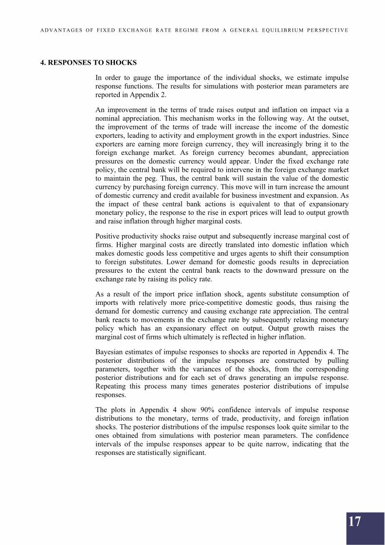
The results on prior and posterior distributions of the model parameters are reported in Appendix 1. Most of posterior distributions are shifted with respect to priors and highly concentrated around their mean values. This implies that overall the data are 1 We construct the posteriors using the Metropolis-Hastings algorithm with a Markov chain 60 000 and
1 000 000 observations long. All estimation was conducted using Dynare 3, in Matlab R2008a.

14
A D V A N T A G E S O F F I X E D E X C H A N G E R A T E R E G I M E F R O M A G E N E R A L E Q U I L I B R I U M P E R S P E C T I V E
informative and the parameter estimates are close to their true values. The only exception where the data provide little information is the interest rate.
To evaluate different exchange rate policies for Latvia, we simulate the model using different policy parameters and compare the results under various policy rules. First we derive results by applying coefficients estimated from the data, i.e., we use ψ1 = 0.515, ψ2 = 0.016, ψ3 = 44.801 and refer to this case as a benchmark model. Table 2 provides the results. Under these parameter values, the exchange rate appears to fit into the existing regime of ±1% band with 99% probability. Furthermore, we simulate a change in the monetary policy by allowing wider exchange rate bands. We consider three different values for ψ3 – 2.0, 1.0, and 0.6 while leaving the rest of the estimated coefficients unchanged. At ψ3 = 2.0, the exchange rate volatility increases 5.9 times, inflation variability amplifies, while interest rate fluctuations become less pronounced which is consistent with the diminishing role of the interest rate in exchange rate stabilisation. Relaxing the bands even further (ψ3 = 1.0), the effect on inflation variation becomes more pronounced. Surprisingly, under wider exchange rate bands output fluctuations amplify, slightly though. This implies that the exchange rate does not serve as a shock absorber.
Finally, we simulate the model for the latter case (ψ3 = 0.6) but allow for different inflation and output gap targeting policies. Column 2 of Table 3 provides results for the case where the inflation coefficient assumes the value commonly associated with the Taylor rule (ψ1 = 1.5), whereas the output gap coefficient is left as derived from the data (ψ2 = 0.016). As expected, inflation targeting brings down inflation fluctuations compared to cases where the central bank demonstrates no concern about the price changes. What is surprising, though: under inflation targeting inflation turns out to be more volatile than under the peg. Under an even tighter inflation targeting regime (ψ1 = 2.0), inflation fluctuations decrease (see Column 3 of Table 3) while still exceeding the respective value of the benchmark model. In the third case, we leave inflation targeting as in the previous case while allowing the central bank to also target the output gap. Additional concern for output stabilisation accounts for lower inflation variability compared to the two other cases covered before while it is still higher than under the existing exchange rate regime with ±1% fluctuation bands.
Table 2 Standard deviations for the benchmark model and various exchange rate regimes
Benchmark model ψ1 = 0.515, ψ2 = 0.016 Variable ψ1 = 0.515, ψ2 = 0.016, ψ3 = 44.801
ψ3 = 2.0 ψ3 = 1.0 ψ3 = 0.6
z 1.605 1.619 1.626 1.630Δe 0.329 1.944 2.880 3.689Δs 1.596 1.626 1.597 1.604π 2.275 7.320 11.104 14.403r 5.518 1.932 1.736 1.701y 5.149 5.262 5.617 5.885
15
A D V A N T A G E S O F F I X E D E X C H A N G E R A T E R E G I M E F R O M A G E N E R A L E Q U I L I B R I U M P E R S P E C T I V E
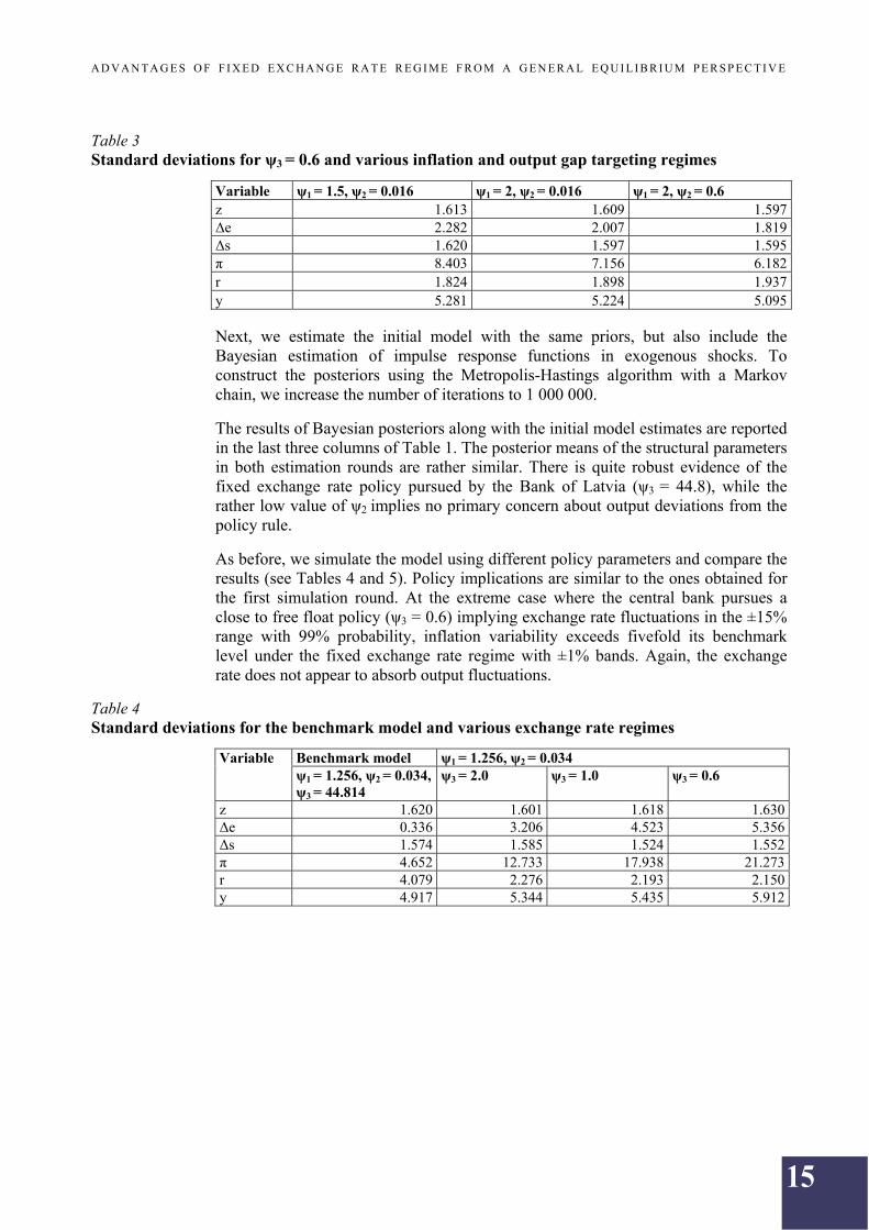
Table 3 Standard deviations for ψ3 = 0.6 and various inflation and output gap targeting regimes
Variable ψ1 = 1.5, ψ2 = 0.016 ψ1 = 2, ψ2 = 0.016 ψ1 = 2, ψ2 = 0.6 z 1.613 1.609 1.597Δe 2.282 2.007 1.819Δs 1.620 1.597 1.595π 8.403 7.156 6.182r 1.824 1.898 1.937y 5.281 5.224 5.095 Next, we estimate the initial model with the same priors, but also include the Bayesian estimation of impulse response functions in exogenous shocks. To construct the posteriors using the Metropolis-Hastings algorithm with a Markov chain, we increase the number of iterations to 1 000 000.
The results of Bayesian posteriors along with the initial model estimates are reported in the last three columns of Table 1. The posterior means of the structural parameters in both estimation rounds are rather similar. There is quite robust evidence of the fixed exchange rate policy pursued by the Bank of Latvia (ψ3 = 44.8), while the rather low value of ψ2 implies no primary concern about output deviations from the policy rule.
As before, we simulate the model using different policy parameters and compare the results (see Tables 4 and 5). Policy implications are similar to the ones obtained for the first simulation round. At the extreme case where the central bank pursues a close to free float policy (ψ3 = 0.6) implying exchange rate fluctuations in the ±15% range with 99% probability, inflation variability exceeds fivefold its benchmark level under the fixed exchange rate regime with ±1% bands. Again, the exchange rate does not appear to absorb output fluctuations.
Table 4 Standard deviations for the benchmark model and various exchange rate regimes
Benchmark model ψ1 = 1.256, ψ2 = 0.034 Variable ψ1 = 1.256, ψ2 = 0.034, ψ3 = 44.814
ψ3 = 2.0 ψ3 = 1.0 ψ3 = 0.6
z 1.620 1.601 1.618 1.630Δe 0.336 3.206 4.523 5.356Δs 1.574 1.585 1.524 1.552π 4.652 12.733 17.938 21.273r 4.079 2.276 2.193 2.150y 4.917 5.344 5.435 5.912

16
A D V A N T A G E S O F F I X E D E X C H A N G E R A T E R E G I M E F R O M A G E N E R A L E Q U I L I B R I U M P E R S P E C T I V E
Table 5 Standard deviations for ψ3 = 0.6 and various inflation and output gap targeting regimes
Variable ψ1 = 1.5, ψ2 = 0.034 ψ1 = 2, ψ2 = 0.034 ψ1 = 2.5, ψ2 = 0.6 z 1.634 1.606 1.625Δe 4.701 4.177 3.321Δs 1.544 1.588 1.545π 18.467 15.950 12.249r 2.186 2.233 2.410y 5.453 5.416 5.179 Results obtained from simulations of various exchange rate regimes and monetary policy rules thus provide some evidence that under the peg inflation variability is lower compared to other policy rules. The model results are therefore in favour of the exchange rate policy currently pursued by the Bank of Latvia. Any changes in the policy would bring unfavourable consequences in terms of macro indicators and loss of credibility to the monetary authority.
17
A D V A N T A G E S O F F I X E D E X C H A N G E R A T E R E G I M E F R O M A G E N E R A L E Q U I L I B R I U M P E R S P E C T I V E
4. RESPONSES TO SHOCKS
In order to gauge the importance of the individual shocks, we estimate impulse response functions. The results for simulations with posterior mean parameters are reported in Appendix 2.
An improvement in the terms of trade raises output and inflation on impact via a nominal appreciation. This mechanism works in the following way. At the outset, the improvement of the terms of trade will increase the income of the domestic exporters, leading to activity and employment growth in the export industries. Since exporters are earning more foreign currency, they will increasingly bring it to the foreign exchange market. As foreign currency becomes abundant, appreciation pressures on the domestic currency would appear. Under the fixed exchange rate policy, the central bank will be required to intervene in the foreign exchange market to maintain the peg. Thus, the central bank will sustain the value of the domestic currency by purchasing foreign currency. This move will in turn increase the amount of domestic currency and credit available for business investment and expansion. As the impact of these central bank actions is equivalent to that of expansionary monetary policy, the response to the rise in export prices will lead to output growth and raise inflation through higher marginal costs.
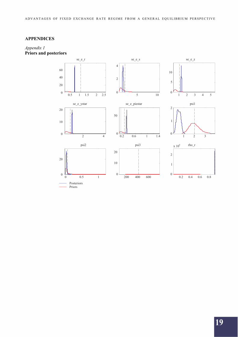
Positive productivity shocks raise output and subsequently increase marginal cost of firms. Higher marginal costs are directly translated into domestic inflation which makes domestic goods less competitive and urges agents to shift their consumption to foreign substitutes. Lower demand for domestic goods results in depreciation pressures to the extent the central bank reacts to the downward pressure on the exchange rate by raising its policy rate.
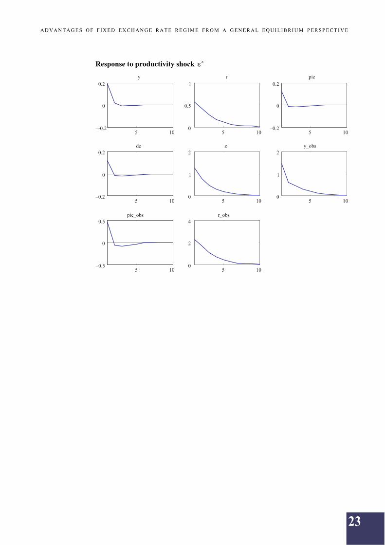
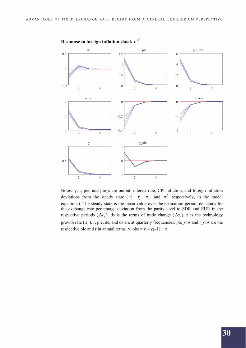
As a result of the import price inflation shock, agents substitute consumption of imports with relatively more price-competitive domestic goods, thus raising the demand for domestic currency and causing exchange rate appreciation. The central bank reacts to movements in the exchange rate by subsequently relaxing monetary policy which has an expansionary effect on output. Output growth raises the marginal cost of firms which ultimately is reflected in higher inflation.
Bayesian estimates of impulse responses to shocks are reported in Appendix 4. The posterior distributions of the impulse responses are constructed by pulling parameters, together with the variances of the shocks, from the corresponding posterior distributions and for each set of draws generating an impulse response. Repeating this process many times generates posterior distributions of impulse responses.
The plots in Appendix 4 show 90% confidence intervals of impulse response distributions to the monetary, terms of trade, productivity, and foreign inflation shocks. The posterior distributions of the impulse responses look quite similar to the ones obtained from simulations with posterior mean parameters. The confidence intervals of the impulse responses appear to be quite narrow, indicating that the responses are statistically significant.

18
A D V A N T A G E S O F F I X E D E X C H A N G E R A T E R E G I M E F R O M A G E N E R A L E Q U I L I B R I U M P E R S P E C T I V E
CONCLUSIONS
In this paper we estimate a small open economy DSGE model for Latvia, following Lubik and Schorfheide (2007) using Bayesian methods. The estimates of the structural parameters fall within plausible ranges. To evaluate different exchange rate policies for Latvia, we simulate the model using different policy parameters and compare the results under various policy rules. In extreme cases where the central bank pursues a close to free float policy, inflation fluctuations exceed fivefold their level under the currently pursued fixed exchange rate regime. Simulation results for the free float regime, allowing for different inflation and output gap targeting policies, suggest that inflation targeting brings down inflation fluctuations compared to cases where the central bank demonstrates no concern for the price changes. What is surprising, however, is that under inflation targeting inflation turns out to be more volatile than under the peg. Additional concern for output stabilisation accounts for lower inflation variability while it is still higher than under the existing exchange rate regime with ±1% fluctuation bands. The model results therefore are in favour of the existing exchange rate policy. Any changes in the policy would bring unfavourable consequences in terms of macro indicators and loss of credibility to the monetary authority.
19
A D V A N T A G E S O F F I X E D E X C H A N G E R A T E R E G I M E F R O M A G E N E R A L E Q U I L I B R I U M P E R S P E C T I V E
APPENDICES
Appendix 1 Priors and posteriors

20
A D V A N T A G E S O F F I X E D E X C H A N G E R A T E R E G I M E F R O M A G E N E R A L E Q U I L I B R I U M P E R S P E C T I V E
Notes: se_e_r, se_e_s, se_e_z, se_e_ystar, and se_e_piestar are standard errors of the
shocks Rt , s
t , zt ,
*yt , and
* t respectively. psi1, psi2, psi3, rho_r, rho_s, rho_z,
rho_ystar, rho_piestar, alpha, lambda, and tau stand for ψ1, ψ2, ψ3, ρr, ρs, ρz, ρy*, ρπ*, α, λ, and τ respectively. r is the steady state real interest rate.

21
A D V A N T A G E S O F F I X E D E X C H A N G E R A T E R E G I M E F R O M A G E N E R A L E Q U I L I B R I U M P E R S P E C T I V E
Appendix 2 Impulse responses to shocks
Response to monetary shock rε

22
A D V A N T A G E S O F F I X E D E X C H A N G E R A T E R E G I M E F R O M A G E N E R A L E Q U I L I B R I U M P E R S P E C T I V E
Response to terms of trade shock sε
Notes: y, r, and pie are output, interest rate and CPI inflation deviations from the steady state ( ty~ , tr , and t , respectively, in the model equations). The steady state is the mean
value over the estimation period. de stands for the exchange rate percentage deviation from the parity level to SDR and EUR in the respective periods ( te ). ds is the terms of
trade change ( ts ). r, pie, de, and ds are at quarterly frequencies. pie_obs and r_obs are
the respective pie and r in annual terms. y_obs = y – y(–1) + z.
23
A D V A N T A G E S O F F I X E D E X C H A N G E R A T E R E G I M E F R O M A G E N E R A L E Q U I L I B R I U M P E R S P E C T I V E
Response to productivity shock zε

24
A D V A N T A G E S O F F I X E D E X C H A N G E R A T E R E G I M E F R O M A G E N E R A L E Q U I L I B R I U M P E R S P E C T I V E
Response to foreign inflation shock *πε
Notes: y, r, pie, and pie_s are output, interest rate, CPI inflation, and foreign inflation deviations from the steady state ( ty~ , tr , t , and *
t respectively, in the model
equations). The steady state is the mean value over the estimation period. de stands for the exchange rate percentage deviation from the parity level to SDR and EUR in the respective periods ( te ). ds is the terms of trade change ( ts ). z is the technology
growth rate ( tz ). r, pie, de, and ds are at quarterly frequencies. pie_obs and r_obs are the
respective pie and r in annual terms. y_obs = y – y(–1) + z.

25
A D V A N T A G E S O F F I X E D E X C H A N G E R A T E R E G I M E F R O M A G E N E R A L E Q U I L I B R I U M P E R S P E C T I V E
Appendix 3
Matrix of covariance of exogenous shocks
Variables rε sε *yε
*πε zε
rε 0.5062 0 0 0 0sε 0 2.5402 0 0 0
*yε 0 0 0.8545 0 0*πε 0 0 0 0.1016 0
zε 0 0 0 0 1.6246
Policy and transition functions
Δe y_obs π_obs r_obs r (–1) –0.156 –0.188 –0.625 0.624
*π (–1) –0.012 0.332 1.642 –0.130z (–1) 0.056 0.696 0.223 1.054y (–1) 0 –1 0 0
*y (–1) 0 –4.560 0 0Δs (–1) –0.020 0.123 0.123 –0.373
rε –0.175 –0,210 –0.698 0.696sε –0.149 0.898 0.898 –2.726
*yε 0 –4,780 0 0*πε –0.028 0.787 3.888 –0.308
zε 0.092 1.148 0.367 1.739
Moments of simulated variables
Variable Mean St. dev. Variance Skewness Kurtosis z 0.031 1.555 2.418 0.014 –0.029Δe –0.002 0.324 0.105 0.066 –0.049Δs 0.011 1.611 2.595 –0.018 –0.159π –0.005 0.574 0.330 –0.055 –0.123π_obs –0.021 2.297 5.276 –0.055 –0.123π* –0.008 0.356 0.127 –0.023 –0.161r 0.009 1.382 1.909 –0.047 0.006r_obs 0.037 5.526 30.541 –0.047 0.006y –2.817 15.527 241.084 –0.238 0.661y_obs 0.028 5.100 26.014 –0.059 –0.218y* 0.590 3.223 10.389 0.219 0.628

26
A D V A N T A G E S O F F I X E D E X C H A N G E R A T E R E G I M E F R O M A G E N E R A L E Q U I L I B R I U M P E R S P E C T I V E
Correlation of simulated variables
Variable z Δe Δs π_obs π* r_obs y_obs y* z 1.000 0.214 –0.013 0.151 0.069 0.553 0.343 –0.062Δe 0.214 1.000 –0.649 –0.130 –0.026 0.521 –0.206 0.009Δs –0.013 –0.649 1.000 0.674 –0.010 –0.823 0.261 –0.016π_obs 0.151 –0.130 0.674 1.000 0.595 –0.548 0.209 –0.042π* 0.069 –0.026 –0.010 0.595 1.000 0.030 0.084 –0.050r_obs 0.553 0.521 –0.823 –0.548 0.030 1.000 –0.003 –0.022y_obs 0.343 –0.206 0.261 0.209 0.084 –0.003 1.000 –0.141y* –0.062 0.009 –0.016 –0.042 –0.050 –0.022 –0.141 1.000
Autocorrelation of simulated variables
Variable 1 2 3 4 5 z 0.603 0.348 0.206 0.107 0.050Δe –0.245 –0.054 –0.046 –0.009 –0.041Δs 0.145 0.062 0.024 0.019 0.005π_obs 0.449 0.134 0.066 0.066 0.045π* 0.457 0.204 0.058 0.034 0.018r_obs 0.426 0.202 0.087 0.035 0.007y_obs –0.010 0.026 –0.019 –0.020 –0.001y* 0.962 0.923 0.884 0.848 0.815

27
A D V A N T A G E S O F F I X E D E X C H A N G E R A T E R E G I M E F R O M A G E N E R A L E Q U I L I B R I U M P E R S P E C T I V E
Appendix 4 Bayesian estimation of impulse responses to shocks (1 000 000 MH simulations)
Response to monetary shock rε

28
A D V A N T A G E S O F F I X E D E X C H A N G E R A T E R E G I M E F R O M A G E N E R A L E Q U I L I B R I U M P E R S P E C T I V E
Response to terms of trade shock sε
Notes: y, r, and pie are output, interest rate and CPI inflation deviations from the steady state ( ty~ , tr , and t respectively, in the model equations). The steady state is the mean
value over the estimation period. de stands for the exchange rate percentage deviation from the parity level to SDR and EUR in the respective periods ( te ). ds is the terms of
trade change ( ts ). r, pie, de, and ds are at quarterly frequencies. pie_obs and r_obs are
the respective pie and r in annual terms. y_obs = y – y(–1) + z.

29
A D V A N T A G E S O F F I X E D E X C H A N G E R A T E R E G I M E F R O M A G E N E R A L E Q U I L I B R I U M P E R S P E C T I V E
Response to productivity shock zε
30
A D V A N T A G E S O F F I X E D E X C H A N G E R A T E R E G I M E F R O M A G E N E R A L E Q U I L I B R I U M P E R S P E C T I V E
Response to foreign inflation shock *πε
Notes: y, r, pie, and pie_s are output, interest rate, CPI inflation, and foreign inflation deviations from the steady state ( ty~ , tr , t , and *
t respectively, in the model
equations). The steady state is the mean value over the estimation period. de stands for the exchange rate percentage deviation from the parity level to SDR and EUR in the respective periods ( te ). ds is the terms of trade change ( ts ). z is the technology
growth rate ( tz ). r, pie, de, and ds are at quarterly frequencies. pie_obs and r_obs are the
respective pie and r in annual terms. y_obs = y – y(–1) + z.

31
A D V A N T A G E S O F F I X E D E X C H A N G E R A T E R E G I M E F R O M A G E N E R A L E Q U I L I B R I U M P E R S P E C T I V E
Appendix 5 Derivation of the small open DSGE model
Households
A representative household of a small open economy maximises its utility given by
00 ),/(
tttt
t NACUE [1]
where Nt denotes hours worked, At is the world technology process, and Ct is a composite consumption index defined as
11
,
11
,
1
)()()1(
tFtHt CCC [2].
CH,t, in its turn, is an index of consumption of domestic goods represented by the CES function
11
0
1
,, )(
djjCC tHtH
where j[0, 1] denotes a differentiated good on the unit interval. CF,t is an index of imported goods defined by
11
0
1
,,
diCC titF
where Ci,t stands for an index of goods imported from country i and consumed by domestic households. As in the case of consumption of domestic goods, the index of imports is given by the CES function
11
0
1
,, )(
djjCC titi .
Parameter 1 implies the elasticity of substitution between goods produced within a specific country. α[0, 1] measures a degree of openness which is commonly defined as share of imports in GDP. Parameter 0 denotes the substitutability between domestic and foreign goods from the standpoint of the domestic consumer, while γ denotes the substitutability between goods imported from different markets.
The household maximises its utility defined in [1] subject to a borrowing constraint
1
0 1
1
0 ,,
1
0 ,, )()()()( tttttttititHtH TNWRDDdjdijCjPdjjCjP [3]
for t = 0, 1, 2, … where PH,t(j) is the price of differentiated domestic good j and Pi,t(j) is the price of differentiated good j imported from country i. Rt is return on
32
A D V A N T A G E S O F F I X E D E X C H A N G E R A T E R E G I M E F R O M A G E N E R A L E Q U I L I B R I U M P E R S P E C T I V E
investment Dt–1 held at the end of period t – 1 (including shares in firms). Finally, Wt
stands for the nominal wage, and Tt denotes lump-sum transfers (taxes).
Solving for optimal allocation between domestic and imported goods renders the respective demand functions
tHtH
tHtH C
P
jPjC ,
,
,,
)()(
[4]
titi
titi C
P
jPjC ,
,
,,
)()(
for i, j [0, 1] where
1
11
0
1,, )( djjPP tHtH refers to the price index of
domestically produced goods and
1
11
0
1,, )( djjPP titi is a price index (in
domestic currency terms) for goods purchased from country i [0, 1]. Substituting definitions of price and quantity indexes PH,t, CH,t, Pi,t, and Ci,t into optimal
allocations in [4] gives tHtHtHtH CPdjjCjP ,,
1
0 ,, )()( and
titititi CPdjjCjP ,,
1
0 ,, )()( .
Optimal choice of imports from country i yields
tFtF
titi C
P
PC ,
,
,,
[5]
for all i[0, 1] where
1
11
0
1,, diPP titF denotes the price index for imported
goods, denominated in domestic currency. Combining the optimality condition in [5] with the definitions of PF,t, and CF,t yields the total expenditures on imported goods
expressed as tFtFtiti CPdiCP ,,
1
0 ,, .
To derive the optimal consumption allocation between domestic and imported goods, we consider profit maximisation problem of firms that buy quantities tHC ,
and tFC , of domestic and foreign produced goods and combine them into a
composite good that is used for consumption by the households. These firms maximise profits in a perfectly competitive environment:
tFtFtHtHttCCC
CPCPCPtFtHt
,,,,,, ,,
max
subject to 11
,
11
,
1
)1(
tFtHt CCC .

33
A D V A N T A G E S O F F I X E D E X C H A N G E R A T E R E G I M E F R O M A G E N E R A L E Q U I L I B R I U M P E R S P E C T I V E
Plugging the constraint into the profit equation and denoting it by f yields
tFtFtHtHtFtHt CPCPCCPf ,,,,
11
,
11
,
1
)1(
.
Derivation of the first-order condition with respect to tHC , results in
01
)1()1(1 ,
1
,
1111
,
11
,
1
,
tHtHtFtHttH
PCCCPC
f
.
Simplifying and using the definition for tC gives
tHtHtt PCCP ,
1
,
11
)1(
or rearranging
tt
tHtH C
P
PC
,
, )1( .
In the same way, derivation of the first-order condition with respect to tFC , implies
tt
tFtF C
P
PC
,
, .
Plugging the derived expressions for tHC , and tFC , into the definition for tC yields
11
,1
1
,1
)1()1(
t
t
tFt
t
tHt C
P
PC
P
PC
or rearranging
,)1()1(
1
,1
1
,1
1
t
t
tFt
t
tHt C
P
PC
P
PC
opening the brackets
1
1
,11
11
,11
1
)1()1(
t
t
tFt
t
tHt C
P
PC
P
PC ,

34
A D V A N T A G E S O F F I X E D E X C H A N G E R A T E R E G I M E F R O M A G E N E R A L E Q U I L I B R I U M P E R S P E C T I V E
cancelling tC and simplifying
1
,
1
,)1(1t
tF
t
tH
P
P
P
P
which yields the equation for the CPI
1
11
,1
, )())(1( tFtHt PPP .
For further convenience, let us rewrite the derived equations
tt
tHtH C
P
PC
,
, )1( ; tt
tFtF C
P
PC
,
, ;
1
11
,1
, )())(1( tFtHt PPP [6].
Thus, total domestic household expenditures on consumption are tttFtFtHtH CPCPCP ,,,, . Given this, one period budget constraint [3] can be
reformulated as
tttttttt TNWRDDCP 1 [7].
To obtain the intratemporal optimality condition, we express the household's utility maximisation problem as a Lagrangian, L:
01
11
00 11
1)/(
tttttttttt
tttt TNWRDDCPNAC
EL
where σ and φ represent household's risk aversion and labour supply aversion respectively.
The relevant first-order conditions are:
011
ttttt
t RED
L 11 tttt RE
011 tttt
t
t
t PCAC
L
.1
1
t
tt
tt C
PA
Eliminating t yields
11
11
1
11
11tt
tt
ttt
tt
t RCPA
ECPA
or
35
A D V A N T A G E S O F F I X E D E X C H A N G E R A T E R E G I M E F R O M A G E N E R A L E Q U I L I B R I U M P E R S P E C T I V E
1111
1t
t
t
tt
ttt
t
t RA
A
PA
PCE
A
C
.
Denotingt
tt A
CC ~
, the latter can be expressed as
1
111
~~t
t
t
t
tttt R
A
A
P
PCEC [8]
which is the Euler equation.
Rearranging the latter yields the one-period stochastic discount factor
1,11
1~
~
tt
t
t
t
t
t
t QA
A
P
P
C
C
[9]
Using )1( tt xXX , log-linearisation of [8] yields
)~1(~
)~1(~
111 tttttttttt raEapEpcERCcC
and making use of the steady state condition R1 which follows from [8], we obtain
tttttttttt raEapEpcEc 111~~
or
}{11~~~~
111111 tttttttttttttttttt aEErcEcraEapEpcEc
[10]
where lowercase letters stand for deviations from the steady state of the respective variables and ttt pp 11 is CPI inflation.
Optimal labour supply choice implies
0
tttt
t
t WNN
L
or substituting for t
ttt
tt NPA
CW
1
tttt
tt
t
t
tt
t NCAP
WN
A
C
AP
W ~
[11].
Denoting tt
tt AP
WW ~
yields

36
A D V A N T A G E S O F F I X E D E X C H A N G E R A T E R E G I M E F R O M A G E N E R A L E Q U I L I B R I U M P E R S P E C T I V E
ttt NCW
~~
which in log-linearised form implies
ttt ncw ~~ [12].
Identities between inflation, exchange rates and terms of trade
Next, several identities linking inflation, exchange rates and terms of trade are defined. Bilateral terms of trade between the domestic economy and country i is given by
tH
titi P
PS
,
,,
which is nothing but the price of country i's goods in terms of home goods. Consequently, the effective terms of trade are defined as
1
11
0
1,
,
, diSP
PS ti
tH
tFt .
Using ttS
t sSeS t 1log1log , where tHtFtt ppSs ,,log , the last
expression can be transformed as
1
11
0 ,
1
11
0 ,
1
11
0
log1
11
0
1, log11log11
1, diSdiSdiediSS titi
Stit
ti
.11log1log11
11
1
0 ,
1
0 ,
1
0 , ttititi sdisdiSdiS
2
Thus the effective terms of trade can be approximated (up to first order) around a symmetric steady state satisfying Si,t = 1 for all i [0, 1] by
1
0 , diss tit [13].
Analogously, log-linearisation of the expression for the CPI around the symmetric steady state gives
tPt eP log
1
11log1log
1
11
,1
, )())(1()())(1(1log1 ,, tFtH PPtFtHtt eePPpP
1
1
,,1
11
,1
, )11()11)(1()log1()log1)(1( tFtHtFtH ppPP
2 We use approximation tt xx 1)1( , where xt is a real number close to zero.

37
A D V A N T A G E S O F F I X E D E X C H A N G E R A T E R E G I M E F R O M A G E N E R A L E Q U I L I B R I U M P E R S P E C T I V E
tFtHtFtH pppp ,,1
1
,, 11)1(1
1111)1(1
tFtH pp ,,)1(1
yielding
ttHtFtHt spppp ,,,)1( [14].
From the last formula it follows that domestic inflation, i.e., the rate of change in the domestic goods price index, 1,,. tHtHtH pp , and CPI inflation are related in the
form
ttHt s , [15]
which implies that the inflation difference is proportional to the percent change in the terms of trade where the coefficient of proportionality is captured by the degree of openness α.
Furthermore, it is assumed that the law of one price holds at a product level both for import and export prices, implying )()( ,,, jPjP i
tititi for all i, j [0, 1]. ti, is the
bilateral nominal exchange rate, i.e., the price of country i's currency in terms of the domestic currency, whereas )(, jPi
ti is the price of country i's good j denominated in
its own currency terms. Applying the law-of-one-price assumption to the definition
of tiP , results in itititi PP ,,, where
1
11
0
1,, )( djjPP iti
iti stands for country i's
domestic price index.
Substituting the same assumption into the expression for PF,t and log-linearising around the symmetric steady state gives
1
1
1
0
1
1
11
0
)(log,
1
1
1
0
1
1
11
0
1,,
1
11
0
1
,,
1
11
0
1,,,
log,
,1
,
)(
1log1
didjedidjjP
diPdiPpPeP
jPti
ititi
ititititFtF
PtF
iti
tF
1
1
1
0
1
1
11
0 ,,
1
1
1
0
1
1
11
0 ,, )(log)1(1)(log)1(1 didjjPdidjjP ititi
ititi
1
1
1
0
11
0 ,,
1
1
1
0
11
0 ,, )(1)(log)1(1
11 didjjpdidjjP i
titiititi
1
11
0
1
,,
1
11
0
1
,log1
11
0
1
,, 1log111 , dipdipedip ititi
iti
ititi
ti

38
A D V A N T A G E S O F F I X E D E X C H A N G E R A T E R E G I M E F R O M A G E N E R A L E Q U I L I B R I U M P E R S P E C T I V E
1
11
0 ,,
1
11
0
1
,,
1
11
0
1
,, 11111 dipedipedipe ititi
ititi
ititi
*1
0 ,,
1
11
0 ,, 1111 tti
titii
titi pedipedipe
or
*1
0 ,,, )( tti
tititF pedipep
where djjpp iti
iti
1
0 ,, )( denotes country i's log domestic price index in terms of its
own currency, 1
0 , diee tit is the log effective nominal exchange rate, and
dipp itit
1
0 ,* stands for the log world price index.
Plugging the terms of trade definition into the last relationship yields
tHttt ppes ,* [16].
The next step is to derive a relationship linking the terms of trade and the real exchange rate. The bilateral real exchange rate with country i is defined as
t
itti
ti P
P,,
, i.e., the ratio of the two countries' CPIs (both denominated in
domestic currency). Defining 1
0 , diqq tit as the log effective real exchange rate,
where titiq ,, log , results in
ttHtttttittit ppsppedippeq ,
*1
0 , )( .
Rewriting the CPI expression in the form
1,
1,
1 )())(1( tFtHt PPP
and dividing both sides by 1,tHP yields
1
1
,
,
1
,
)1()1( ttH
tF
tH
t SP
P
P
P
or
1
1
1
,
])1[( ttH
t SP
P.
Log-linearising the latter around a symmetric steady state
39
A D V A N T A G E S O F F I X E D E X C H A N G E R A T E R E G I M E F R O M A G E N E R A L E Q U I L I B R I U M P E R S P E C T I V E
,1log111
11
1
11
1
1
]11log[1
1])1log[(
1
1logloglog
log11
11,,
,
ttS
t
tttHttHttH
t
sSeS
SSppPPP
P
t
which results in ttHt spp , , and plugging in the last expression for tq yields
tttHttttt sppsppeq )1(,* [17].
Furthermore, a few identities related to international risk sharing are derived. Condition [9] which characterises the domestic economy must also hold for any country i, accounting for the exchange rate
1,
111
1~
~
tti
t
it
t
ti
t
it
it
it Q
A
A
P
P
C
C
[18].
Equating left hand sides of [9] and [18] and using definition of the real exchange rate yields
it
it
it
it
t
t
it
it
t
t
t
t
t
t
P
P
A
A
C
C
P
P
A
A
C
C
111
1
11
1~
~
~
~
,
ii
i
i
it
t
it
it
tit
t
it
it
t constP
P
C
C
P
P
C
C
P
P
C
C
0
0
0
0
01
1
1
1
1~
~...~
~
~
~
which is referred to as the "initial consumption ratio".
Rearranging yields
1
,
1
,1
~~1~ti
ititi
it
i
t CCconst
C [19]
where i is a constant which depends on initial conditions regarding relative net asset
positions. Assuming symmetric initial conditions, i.e., zero net foreign asset holdings and an ex-ante identical environment, 1i for all i.
Expressing [19] in logs
tii
ttiitti
ittt qcCCcC ,,
1
,
1~log1~
log~
log~~log
and integrating over i results in
tttttii
ttt scqcdiqdiccdic
1~1~1~~~ **
1
0
,
1
0
1
0
[20]
40
A D V A N T A G E S O F F I X E D E X C H A N G E R A T E R E G I M E F R O M A G E N E R A L E Q U I L I B R I U M P E R S P E C T I V E
where 1
0
* ~~ dicc itt stands for stationary log world consumption, and the second
equality is obtained by substituting the expression for qt.from [17]. The derived equation relates domestic consumption with world consumption and terms of trade.
Firms
The domestic economy is populated by a continuum of firms j[0, 1], where each one produces a differentiated good using the same technology, represented by the production function
)()( jNAjY ttt
where At is the level of technology and tt Aa log is described by the AR(1)
process ttat vaa 1 .
All firms face identical demand curves and take the aggregate price level and aggregate consumption index exogenously. Following the price setting mechanism proposed by Calvo (1983), each firm may change its price with probability 1 – θ every period, irrespective of the last time of adjustment. Thus, each period a fraction 1 – θ of firms reset their prices, whereas the rest θ keep their prices unchanged. In this way, θ represents price stickiness.
Next, the aggregate price level dynamics is described. Given that all firms resetting prices will choose the same price tHP , , the aggregate price level takes the form
1
11
,1
1,, ))(1()( tHtHtH PPP .
Dividing both sides by 1, tHP yields
1
1,
,1, )1(
tH
tHtH P
P [21]
where 1,
,,
tH
tHtH P
P is the gross inflation rate between t – 1 and t of the
domestically produced goods. Given that in a steady state with zero inflation
tHtHtH PPP ,1,, for all t, log-linearisation of the last expression around the
steady state results in
))(1( 1,,, tHtHtH pp [22].
Equation [22] implies that inflation results from firms re-optimising their price each period so that it differs from the average t – 1 period price in the economy. Therefore, to follow the inflation dynamics in the course of time, the next step is to clarify the factors underlying firms' price setting decisions.

41
A D V A N T A G E S O F F I X E D E X C H A N G E R A T E R E G I M E F R O M A G E N E R A L E Q U I L I B R I U M P E R S P E C T I V E
A firm re-optimising in period t will choose the price tHP , to maximise the present
market value of its profits generated while the price remains effective
0)(max0
,,,
ktktkttkttHkttt
k
PYYPQE
tH
subject to the set of demand constraints
tHd
ktktHktH
tHiktHktH
ktH
tHtkt PYC
P
PdiCC
P
PY ,,
,
,1
0
,,,
, ˆ
[23]
for k = 0, 1, 2, … where )/)(/()~
/~
(, kttktttktk
ktt PPAACCQ
is the
stochastic discount factor for nominal payoffs described above, )(t is the cost
function, and tktY denotes the t + k period output of a firm that last reset its price in
period t.
Plugging the expression for tktY from [23] into the profit maximisation equation
and denoting it by L yields
0,
,
,,, )(ˆ
ktktktktH
ktH
tHtHkttt
k YCP
PPQEL
0,
,
,,
,
1
,,ˆˆ1
kktH
ktH
tHktktH
ktHtHkttt
k CP
PC
PPQE
.
The first order condition with respect to tHP , implies
0ˆ)(
)()(ˆ)1(
0,
,
1,
,,
,,
,
kktH
ktH
tHtktktH
ktH
tHkttt
k
tH
CP
PC
P
PQE
P
L
or using [23]
0)1(0 ,
,
k tH
tkt
tkttktktttk
P
YYQE .
Multiplying both terms by )1/(, tHP gives
0)}({0
,,
ktkttHtktkttt
k PYQE [24]
42
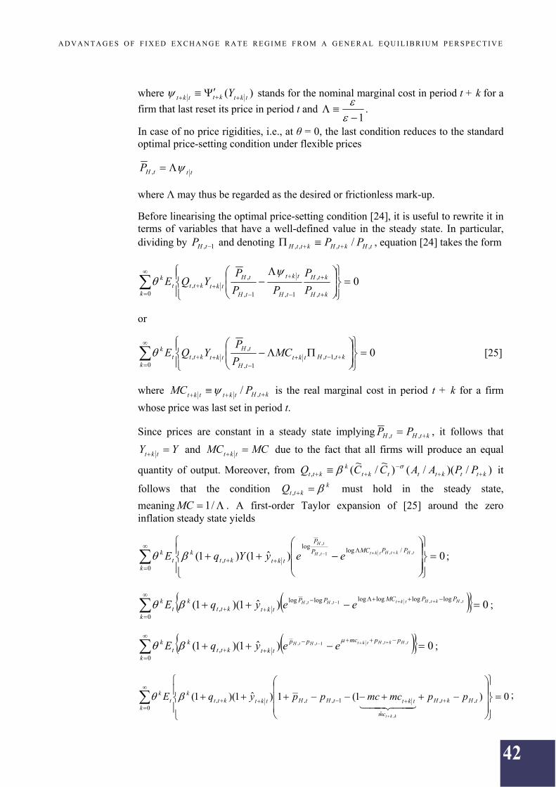
A D V A N T A G E S O F F I X E D E X C H A N G E R A T E R E G I M E F R O M A G E N E R A L E Q U I L I B R I U M P E R S P E C T I V E
where )( tktkttkt Y stands for the nominal marginal cost in period t + k for a
firm that last reset its price in period t and 1
.
In case of no price rigidities, i.e., at θ = 0, the last condition reduces to the standard optimal price-setting condition under flexible prices
tttHP ,
where Λ may thus be regarded as the desired or frictionless mark-up.
Before linearising the optimal price-setting condition [24], it is useful to rewrite it in terms of variables that have a well-defined value in the steady state. In particular, dividing by 1, tHP and denoting tHktHkttH PP ,,,, / , equation [24] takes the form
00 ,
,
1,1,
,,
k ktH
ktH
tH
tkt
tH
tHtktkttt
k
P
P
PP
PYQE
or
00
,1,1,
,,
kkttHtkt
tH
tHtktkttt
k MCP
PYQE [25]
where ktHtkttkt PMC ,/ is the real marginal cost in period t + k for a firm
whose price was last set in period t.
Since prices are constant in a steady state implying ktHtH PP ,, , it follows that
YY tkt and MCMC tkt due to the fact that all firms will produce an equal
quantity of output. Moreover, from )/)(/()~
/~
(, kttktttktk
ktt PPAACCQ
it
follows that the condition kkttQ , must hold in the steady state,
meaning /1MC . A first-order Taylor expansion of [25] around the zero inflation steady state yields
0)ˆ1()1(0
/loglog
,,,1,
,
k
PPMCP
P
tktkttk
tk tHktHtkttH
tH
eeyYqE ;
0)ˆ1)(1(0
loglogloglogloglog,
,,1,,
k
PPMCPP
tktkttk
tk tHktHtkttHtH eeyqE ;
0)ˆ1)(1(0
,,,1,,
k
ppmcpp
tktkttk
tk tHktHtkttHtH eeyqE
;
0)1(1)ˆ1)(1(0
,,
ˆ
1,,,
,
ktHktH
cm
tkttHtHtktkttk
tk ppmcmcppyqE
kkt
;

43
A D V A N T A G E S O F F I X E D E X C H A N G E R A T E R E G I M E F R O M A G E N E R A L E Q U I L I B R I U M P E R S P E C T I V E
0)(ˆ)ˆ1)(1(0
1,,1,,,
ktHktHtkttHtHtktktt
kt
k ppcmppyqE .
Since in the steady state
0)(ˆ 1,,1,, tHktHtkttHtH ppcmpp ,
it follows that
0)(ˆ0
1,,1,,
ktHktHtkttHtH
kt
k ppcmppE ;
or rearranging
0)(ˆ0
1,,0
1,,
ktHktHtkt
kt
k
k
kktHtH ppcmEpp .
Using
1
1
0k
kk , the latter yields
0)(ˆ1 0
1,,1,,
ktHktHtkt
kt
ktHtH ppcmEpp
or
})({)()1( 1,,0
1,,
tHktHtktt
k
ktHtH ppmcEpp [26]
where mcmcmc tkttkt
stands for the log deviation of marginal cost from its
steady state value mc and log is the log of the desired gross mark-up.
Equilibrium
The demand side
Goods market clearing in the domestic economy requires
diA
jC
A
jC
A
jY
t
itH
t
tH
t
t 1
0
,, )()()(
for all j[0, 1] and all t where )(, jC itH stands for country i's demand for the
domestically produced good j.
Let us denote ;)(
)(~
t
tt A
jYjY ;
)()(
~ ,,
t
tHtH A
jCjC
t
itHi
tH A
jCjC
)()(
~ ,, .
Using [4] and [6], domestic consumption can be rewritten in the form

44
A D V A N T A G E S O F F I X E D E X C H A N G E R A T E R E G I M E F R O M A G E N E R A L E Q U I L I B R I U M P E R S P E C T I V E
)6(
,
,
,
)4(
,,
,, )1(
)()()( t
t
tH
tH
tHtH
tH
tHtH C
P
P
P
jPC
P
jPjC
or
tt
tH
tH
tHtH
tH
tHtH C
P
P
P
jPC
P
jPjC
~)1(
)(~)()(
~ ,
,
,,
,
,,
.
Assuming symmetric preferences across countries and using [4], [5], and [6], country i's demand for the domestically produced good j can be expressed as
iti
t
itF
itFti
tH
tH
tHitH C
P
P
P
P
P
jPjC
~)()(
~ ,
,,
,
,
,,
.
Plugging the last two expressions into the goods market clearing equation yields
1
0
,
,,
,,
,
, )1()()(
diA
C
P
P
P
P
A
C
P
P
P
jP
A
jY
t
it
it
itF
itFti
tH
t
t
t
tH
tH
tH
t
t
or
1
0
,
,,
,,
,
, ~~)1(
)()(
~diC
P
P
P
PC
P
P
P
jPjY i
tit
itF
itFti
tHt
t
tH
tH
tHt
[27].
Substituting [27] into the aggregate domestic output equation given by
11
0
11
)(~~
djjYY tt gives
1
1
0
11
1
0
,
,,
,,
1
,
, ~~)1(
)(~
djdiC
P
P
P
PC
P
P
P
jPY i
tit
itF
itFti
tHt
t
tH
tH
tHt
1)(1
)()(1)(
)(1
11
0
1,
,
1
11
0
1,,
11
0
1,
,
11
0
1
,
,
djjPP
djjPPdjjPP
djP
jP
tH
tH
tHtHtH
tHtH
tH

45
A D V A N T A G E S O F F I X E D E X C H A N G E R A T E R E G I M E F R O M A G E N E R A L E Q U I L I B R I U M P E R S P E C T I V E
1
0
,
,,
,, ~~)1( diC
P
P
P
PC
P
P iti
t
itF
itFti
tHt
t
tH
t
itti
tiiti
ttti
tH
itFti
tH
itFti
tt
tH
iti
t
itF
t
tH
tH
itFti
tt
tH
P
PdiC
PPP
P
P
PC
P
P
diCP
P
P
P
P
PC
P
P
,,
1
0
,,
,,
,
,,,
1
0
,,
,
,,,
~11~)1(
~~)1(
1
,
1
,
1
0
,,
,,, ~~~~)19(
~~)1( tit
itti
itt
itti
tH
itFti
tt
tH CCCCdiCP
PC
P
P
1
0
1
,,
,,
,
,, ~~)1(
,
diCP
P
P
PC
P
Ptti
S
ti
itFti
S
tH
tit
t
tH
itti
1
0
1
,,, )1(
~diSSC
P
Ptiti
itt
t
tH
[28]
where the last equality follows from [19], and where itS denotes country i's effective
terms of trade, while tiS , stands for the bilateral terms of trade between the domestic
economy and country i.
Given 01
0 dis i
t , the first-order log-linear approximation to [28] around the steady
state implies
1
0
1
,,,~
log )1(~~1
~log1
~diSSC
P
PyYeY titi
itt
t
tHtt
Yt
t
1
0
,,, log1
1loglog1)1(~
log1loglog1 diSSCPP titiittttH
1
0
,,
)14(
,
111)1(~11 diqsscpp titi
itt
s
ttH
t
1
0
,
1
0
,
11)1(~11 diqdiscs tititt

46
A D V A N T A G E S O F F I X E D E X C H A N G E R A T E R E G I M E F R O M A G E N E R A L E Q U I L I B R I U M P E R S P E C T I V E
tttttttt qsscqscs
1~1
11~11
ttt qsc
1~1
which yields
ttttttttttt scsscsqqscy
~1
1~11~~ [29]
where )1)(1( .
Condition [29] applies to all countries, therefore for country i it takes the form
it
it
it scy
~~ . Summing up all countries, we obtain the world market clearing
condition
*1
0
1
0
* ~~~~t
it
itt cdicdiyy [30]
where *~ty and *~
tc are stationary world output and consumption (in log terms),
whereas the market clearing equality derives from the fact that 01
0 dis i
t .
Substituting the expression for ct from [20] into [29] and using equality [30] implies
ttttttttttt sysscsccscy
1~1~1~~)20(~~ ***
or
ttt syy
1~~ * [31]
where 0)1(1
.
Expressing [29] for t + 1 and using Euler equation [10] to substitute for Et{ct+1} results in
}{}{1
}){(1~~~)30(
}{}{1
}){(1~}{}~{}~{
111
111111
tttttttttttt
tttttttttttttt
sEaEErsysyc
sEaEErcsEcEyE
or
47
A D V A N T A G E S O F F I X E D E X C H A N G E R A T E R E G I M E F R O M A G E N E R A L E Q U I L I B R I U M P E R S P E C T I V E
)1(
})~~{(}{
1}){(
)1(
1}~{
}~~{}{)~~()32(
}{}{1
}){(1
}~{
}{}{1
}){(1
}~{
}{}{)15(
}{}{1
}){(1
}~{~
*11
11,1
*111
*
111,1
1111,1
11,1
1111
ttttttHtttt
tttattttat
tttttHtttt
ttttttHtttt
ttHttt
tttttttttt
yyEaEEryE
yyEsEyys
sEaEEryE
sEaEsEryE
sEE
sEaEEryEy
)1(
~
)1(
}~{}{
1}){(
)1(
1}~{
*11
11,1
tttttttHtttt
yEyEaEEryE .
Rearranging yields
)1(
}{1
}){()1(
1
)1(
}~{}~{0
*1
11,1
1
tttttHtt
tttt
yEaEEr
yEyE ;
;
)1(
~}{
1}){(
)1(
1
)1(
1}~{
)1(
~}{
1}){(
)1(
1
)1(1}~{0
*1
11,1
*1
11,1
tttttHtttt
tttttHtttt
yEaEEryE
yEaEEryE
*111,1
~}{)1(1
}){(1
}~{0 tttttHtttt yEaEEryE
;
*111,1
~}{)1(1
}){(1
}~{~ tttttHttttt yEaEEryEy
[32]
where 1)1)(1()1( .
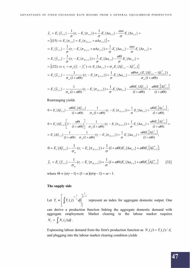
The supply side
Let 11
11
0)(
djjYY tt represent an index for aggregate domestic output. One
can derive a production function linking the aggregate domestic demand with aggregate employment. Market clearing in the labour market requires
1
0)( djjNN tt .
Expressing labour demand from the firm's production function as ttt AjYjN /)()(
and plugging into the labour market clearing condition yields

48
A D V A N T A G E S O F F I X E D E X C H A N G E R A T E R E G I M E F R O M A G E N E R A L E Q U I L I B R I U M P E R S P E C T I V E
1
0
1
0
1
0
)()()(dj
Y
jY
A
Ydj
AY
YjYdj
A
jYN
t
t
t
t
tt
tt
t
tt
or using [4]
1
0
)(dj
P
jP
A
YN
t
t
t
tt
.
Taking logs,
tttt dnay
where 1
0)/)((log djPjPd ttt
. In a neighbourhood of the zero inflation steady
state, dt is equal to zero up to a first-order approximation, therefore the last relationship reduces to
ttt nay [33].
To get the inflation equation, it is useful to rewrite [26] taking into account that the
condition kttkt mcmc holds for the Cobb-Douglas production function Yt = AtNt.
The condition implies equal marginal costs both for firms which reoptimise their price and for the rest.
})({)()1( 1,,
01,, tHktHktt
k
ktHtH ppmcEpp
})({)()1()()1( 1,,1
1,,
tHktHktt
k
ktHtHt ppmcEppmc
})({)()1()1( 1,,,1,1
0, tHtHtHktHktt
k
ktHt ppppmcEmc
)}()({)()1()1()1( 1,,,1,1
0, tHtHtHktHktt
k
ktHt ppppmcEmc
tHtHtmc ,,)1(
01,,,1,1
0
)()1()()}({)()1(
,k
ktHtHtHktHktt
k
k
tH
ppppmcE
tHtHktHkttk
ktHtHt ppmcEmc ,,1,1
0,, )}({)()1()1(
or

49
A D V A N T A G E S O F F I X E D E X C H A N G E R A T E R E G I M E F R O M A G E N E R A L E Q U I L I B R I U M P E R S P E C T I V E
tHttHktHkttk
ktHtH mcppmcEpp ,,1,1
01,, )1()({)()1(
[33'].
Rewriting [26] for )( ,1, tHtH pp yields
})({)()1( ,1,110
,1, tHktHkttk
ktHtH ppmcEpp
.
Estimating expectation gives
})({)()1( ,1,1
0,1, tHktHktt
k
ktHtHt ppmcEppE
[33''].
Plugging [33"] into [33'] yields
tHttHtHttHtH mcppEpp ,,1,1,, )1()(
[34].
Using [22], equation [34] implies
tHttHttH mcE ,1,, )1(1
1
1
1
or
ttHttHtHtH mcE
)1(1
1
11
11,,,,
.
This yields domestic inflation as a function of deviations of marginal cost from its steady state value
ttHttH mcE
}{ 1,, [35]
where
)1)(1(
.
Equation [35] implies that inflation of domestically produced goods is not affected by parameters referring to the open economy. Conversely, real marginal cost as a function of domestic output in the open economy does differ from the closed economy case which results from the wedge between output and consumption, and between domestic and consumer prices. To show this is the case, let us first define real marginal cost (in terms of deviation from the steady-state) as a difference between real wage and marginal product of labour, mpnt,
ttHtt mpnpwmc
)( , .
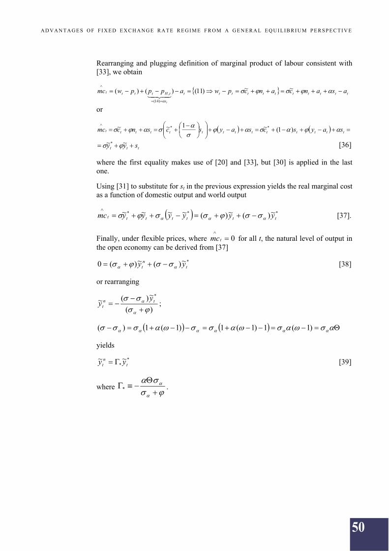
50
A D V A N T A G E S O F F I X E D E X C H A N G E R A T E R E G I M E F R O M A G E N E R A L E Q U I L I B R I U M P E R S P E C T I V E
Rearranging and plugging definition of marginal product of labour consistent with [33], we obtain
ttttttttttt
s
tHtttt asancancpwapppwmc
t
~~)11()()(
)14(
,
or
tttttttttttttt sayscsayscsncmc )1(~1~~ **
ttt syy ~~* [36]
where the first equality makes use of [20] and [33], but [30] is applied in the last one.
Using [31] to substitute for st in the previous expression yields the real marginal cost as a function of domestic output and world output
*** ~)(~)(~~~~ttttttt yyyyyymc
[37].
Finally, under flexible prices, where 0
tmc for all t, the natural level of output in the open economy can be derived from [37]
*~)(~)(0 tnt yy [38]
or rearranging
)(
~)(~*
tnt
yy ;
)1(1)1(1)1(1)(
yields
**~~
tnt yy [39]
where
* .

51
A D V A N T A G E S O F F I X E D E X C H A N G E R A T E R E G I M E F R O M A G E N E R A L E Q U I L I B R I U M P E R S P E C T I V E
A simplified version
In the paper, we estimate a simplified version of Gali and Monacelli (2005) model presented above where ,0 ,1 ,1 and /1 . The open economy model consists of a forward-looking IS equation and the New Keynesian Phillips curve. Monetary policy is defined by an interest rate rule, whereas the exchange rate is introduced via the CPI equation given that PPP holds.
First, the Phillips curve is derived. Subtracting [38] from [37] yields
)~~)((~)(~)(~)(~)( ** nttt
ntttt yyyyyymc
[40].
Substituting [40] and 0 into [35] gives
)~~(}{}{ 1,1,,ntttHtttHttH yyEmcE
[41].
Recalling that )1(1
and )1)(1()1(1 which,
under assumption ,1 1 , becomes
)2(1
11
)1(11
1
[42]
and plugging the latter into the definition for yields
)2)(1(
1
)2(1
1
/1
[43].
Substituting [43] into [41] leads to the New Keynesian Phillips curve in terms of domestic goods inflation
)~~()2)(1(
}{)~~(}{ 1,1,,ntttHt
ntttHttH yyEyyE
[44].
To derive [44] via the CPI inflation we use [15]. In contrast to Gali and Monacelli (2005) we define terms of trade as the relative price of exports in terms of imports, therefore CPI and domestic inflation are now related in the form
tttH s ,
and for t + 1
}{}{}{ 111, tttttHt sEEE .
Substituting the last two expressions for tH , and }{ 1, tHtE into [44] results in
)~~()2)(1(
}{}{ 11ntttttttt yysEEs

52
A D V A N T A G E S O F F I X E D E X C H A N G E R A T E R E G I M E F R O M A G E N E R A L E Q U I L I B R I U M P E R S P E C T I V E
or rearranging
)~~()1)(2(
}{}{ 11ntttttttt yyssEE
,
where the natural rate of output follows from [39]
*****
~)1)(2(~~~~tttt
nt yyyyy
.
Next, the IS curve is derived. Plugging )2(1
1
,
)2)(1(1
, and }{}{}{ 111, tttttHt sEEE into [32] yields
*11111
~1)2(}{)2(
11}){))(2)(1((}~{~
ttttttttttt yEaEsEryEy
*
11111~1
)2(}{)2)(1(}){))(2)(1((}~{ tttttttttt yEaEsEryE
*11111
~1)2(}){}{))(2)(1((}~{
tttttttttt yEaEsEryE .
Given that zt is the growth rate of the world technology process At, i.e., tt za ,
where tt Aa log , and is described by the AR(1) dynamics zttzt zz 1 , we
obtain
tztttt zzEaE }{}{ 11 .
Plugging the last derivation into the expression for ty~ yields the IS equation
*1111
~1)2()}{))(2)(1((}~{~
tttzttttttt yEzsEryEy .

53
A D V A N T A G E S O F F I X E D E X C H A N G E R A T E R E G I M E F R O M A G E N E R A L E Q U I L I B R I U M P E R S P E C T I V E
BIBLIOGRAPHY
Calvo, Guillermo A. (1983) – Staggered Prices in a Utility-Maximising Framework. Journal of Monetary Economics, vol. 12, No. 3, September, pp. 383–398.
Christiano, Lawrence J., Eichenbaum, Martin, Evans, Charles (2005) – Nominal Rigidities and the Dynamic Effects of a Shock to Monetary Policy, Journal of Political Economy, vol. 113, No. 1, February, pp. 1–45.
Del Negro, Marco, Schorfheide, Frank, Smets, Frank, Wouters, Raf (2005) – On the Fit and Forecasting Performance of New Keynesian Models. Centre for Economic Policy Research Discussion Paper, No. 4848, January.
Gali, Jordi, Gertler, Mark (1999) – Inflation Dynamics: A Structural Econometric Analysis. Journal of Monetary Economics, vol. 44, No. 2, October, pp. 195–222.
Gali, Jordi, Monacelli, Tommaso (2005) – Monetary Policy and Exchange Rate Volatility in a Small Open Economy, Review of Economic Studies, vol. 72, No. 3, July, pp. 707–734.
Hradiský, Martin, Girardi, Riccardo, Ratto, Marco (2007) – Think Twice, the EMU has its Price: The Czech Republic Case. Preliminary and incomplete, September.
Kydland, Finn, Prescott, Edward (1982) – Time to Build and Aggregate Fluctuations. Econometrica, vol. 50, No. 6, November, pp. 1345–1370.
Kydland, Finn, Prescott, Edward (1996) – The Computational Experiment: An Econometric Tool. Journal of Economic Perspectives, vol. 10, No. 1, Winter, pp. 69–85.
Lubik, Thomas A., Schorfheide, Frank (2007) – Do Central Banks Respond to Exchange Rate Movements? A Structural Investigation. Journal of Monetary Economics, vol. 54, No. 4, May, pp. 1069–1087.
Rotemberg, Julio J., Woodford, Michael (1997) – An Optimisation-Based Econometric Framework for the Evaluation of Monetary Policy. NBER Macroeconomic Annual, vol. 12, pp. 297–361.
Sbordone, Argia M. (2002) – Prices and Unit Labor Costs: A New Test of Price Stickiness. Journal of Monetary Economics, vol. 49, No. 2, March, pp. 265–292.
Smets, Frank, Wouters, Raf (2003) – An Estimated Dynamic Stochastic General Equilibrium Model for the Euro Area. Journal of the European Economic Association, vol. 1, No. 5, September, pp. 1123–1175.
Smets, Frank, Wouters, Raf (2004) – Forecasting with a Bayesian DSGE Model: an Application to the Euro Area. ECB Working Paper, No. 389, September.