TOPOLOGY OPTIMIZATION OF TENSEGRITY …archive/pdf/e_mag/Vol.55_02_125.pdf · cables of a tensegrity structure. Finding new topologies of ... and cell cytoskeleton models in biomechanics

Journal of the Operations Research Society of Japan c⃝ The Operations Research Society of JapanVol. 55, No. 2, June 2012, pp. 125–145

TOPOLOGY OPTIMIZATION OF TENSEGRITY STRUCTURES UNDER

SELF-WEIGHT LOADS

Yoshihiro KannoUniversity of Tokyo

(Received November 11, 2011)

Abstract A tensegrity structure is a prestressed pin-jointed structure consisting of continuously connectedtensile members (cables) and disjoint compressive members (struts). This paper addresses topology opti-mization of tensegrity structures subjected to self-weight loads, where the compliance, i.e., the strain energyat the equilibrium state, is to be minimized. It is shown that the optimization problem can be formulatedas a mixed integer linear programming (MILP) problem. The proposed method does not require connectiv-ity relation of cables and struts of a tensegrity structure to be known in advance. Numerical experimentsillustrate that various tensegrity structures can be found by solving the presented MILP problem.

Keywords: Optimization, mixed integer programming, structural optimization, tenseg-rity, tension structure, design-dependent constraint

1. Introduction

The terminology tensegrity , coined by Fuller [13] from tension integrity , represents a partic-ular class of tension structures invented by Richard Buckminster Fuller [12], David GeorgesEmmerich [11], and Kenneth Snelson [30]. A tensegrity structure is a prestressed pin-jointedstructure consisting of continuous tensile members (cables) and discontinuous compressivemembers (struts). An example of a tensegrity structure is shown in Figure 1. This tenseg-rity structure consists of three struts and nine cables connected by six nodes, where strutsand cables are depicted by thick and thin lines, respectively. Here, struts do not touch eachother, while cables are connected continuously. The nodes are aligned in the shape of atwisted triangular prism. By introducing an axial tensile force to each cable, this tensegritystructure attains a stable equilibrium state. The forces introduced at this initial equilibriumstate are called the prestress forces .

Since cables of a tensegrity structure are very thin compared with struts, tensegritystructures often give the impression of a cluster of struts floating in the air. Snelson hasbeen creating many tensegrity structures as fascinating sculptures [31] with his intuition asan artist and sophisticated techniques developed over the years. Fuller and Emmerich, incontrast, explored possibility of application of tensegrity structures to architecture. This at-tempt, afterward, has been realized as, e.g., tensegrity domes [25]. Following these pioneers,various methods for finding forms of tensegrity structures have been proposed by many re-searchers; see surveys due to Juan and Mirats Tur [20] and Tibert and Pellegrino [35]. Notethat an arbitrarily given geometrical configuration is not necessarily realized as a tenseg-rity structure because the configuration of a tensegrity structure depends on the prestressforces. Most of the proposed numerical methods require to specify topology of a tenseg-rity structure as input data, where by topology we mean the connectivity of struts andcables of a tensegrity structure. Finding new topologies of tensegrity structures has been

125

126 Y. Kanno

Figure 1: An example of a tensegrity structure

fully addressed only by few authors and remains as a challenging problem. For example,based on the group representation theory [8], Back and Connelly [3] attempted to enumeratetensegrity structures with the specified symmetry property. There exist only few numericalmethods that can find asymmetric topology of tensegrity structures [10, 21, 26].

Today the original definition of tensegrity has been extended in various ways; see Motro[24] and the references therein. It has been recognized, or at least expected, that potentialapplications of tensegrity structures include architectural and civil engineering structures [1,4, 25], deployable structures [33, 34], and cell cytoskeleton models in biomechanics [36, 37].They are also studied in the graph theory [5, 19, 32].

On the basis of this overview, it is desired to develop numerical methods that can findvarious topologies of tensegrity structures without experience and intuition. The authorproposed a mixed integer linear programming (MILP) approach to topology optimizationof compliance of a tensegrity structure subjected to a fixed external load [21]. In continu-ation of that previous work, this paper addresses self-weight loading. The self-weight loaddepends on design of a structure and design is certainly unknown in the course of optimiza-tion. Therefore, topology optimization of structures with the self-weight loads possessesparticular difficulties. This problem was discussed by Rozvany [27] for the plastic design,and subsequently studied for arches [28], beams and columns [2, 22, 29], composite struc-tures [23], shell structures [18], and continua [6]. Nevertheless, the self-weight load is stilloften neglected in optimization of structures. However, tensegrity structures are unusualstructures in the sense that stiff structural elements, i.e., struts, are not connected to eachother, and hence they are relatively flexible in general. Therefore, it is important to con-sider the self-weight load, which might significantly affect the equilibrium configuration ofa tensegrity structure. It is often that the compliance, i.e., the external work done by anapplied load, is used as a measure of global flexibility of a structure. Hence, by minimizingthe compliance under the self-weight load we can find a tensegrity structure which is stiffagainst the self-weight load.

The paper is organized as follows. Section 2 introduces the definition and fundamentalequations of tensegrity structures. The terminology of the graph theory is used in thisexposition, especially for readers who are familiar with operations research but not withapplied mechanics. Section 3 presents the constraints and the objective function consideredin the topology optimization of tensegrity structures. In Section 4, the optimization problemis reduced to an MILP problem. Three numerical examples are demonstrated in Section 5.We conclude in Section 6.

Copyright c⃝ by ORSJ. Unauthorized reproduction of this article is prohibited.

Tensegrity Optimization for Self Weight 127

2. Fundamentals of Tensegrity Structures

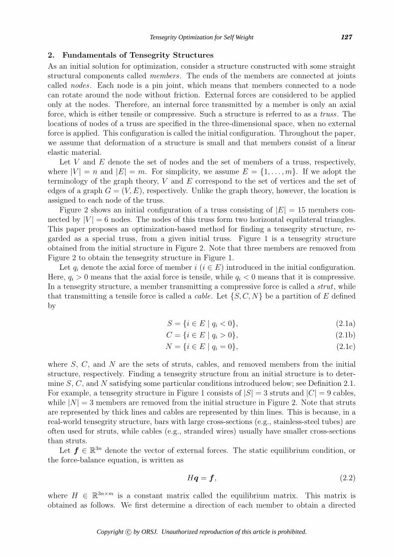
As an initial solution for optimization, consider a structure constructed with some straightstructural components called members . The ends of the members are connected at jointscalled nodes . Each node is a pin joint, which means that members connected to a nodecan rotate around the node without friction. External forces are considered to be appliedonly at the nodes. Therefore, an internal force transmitted by a member is only an axialforce, which is either tensile or compressive. Such a structure is referred to as a truss . Thelocations of nodes of a truss are specified in the three-dimensional space, when no externalforce is applied. This configuration is called the initial configuration. Throughout the paper,we assume that deformation of a structure is small and that members consist of a linearelastic material.

Let V and E denote the set of nodes and the set of members of a truss, respectively,where |V | = n and |E| = m. For simplicity, we assume E = {1, . . . ,m}. If we adopt theterminology of the graph theory, V and E correspond to the set of vertices and the set ofedges of a graph G = (V,E), respectively. Unlike the graph theory, however, the location isassigned to each node of the truss.

Figure 2 shows an initial configuration of a truss consisting of |E| = 15 members con-nected by |V | = 6 nodes. The nodes of this truss form two horizontal equilateral triangles.This paper proposes an optimization-based method for finding a tensegrity structure, re-garded as a special truss, from a given initial truss. Figure 1 is a tensegrity structureobtained from the initial structure in Figure 2. Note that three members are removed fromFigure 2 to obtain the tensegrity structure in Figure 1.

Let qi denote the axial force of member i (i ∈ E) introduced in the initial configuration.Here, qi > 0 means that the axial force is tensile, while qi < 0 means that it is compressive.In a tensegrity structure, a member transmitting a compressive force is called a strut , whilethat transmitting a tensile force is called a cable. Let {S,C,N} be a partition of E definedby

S = {i ∈ E | qi < 0}, (2.1a)

C = {i ∈ E | qi > 0}, (2.1b)

N = {i ∈ E | qi = 0}, (2.1c)

where S, C, and N are the sets of struts, cables, and removed members from the initialstructure, respectively. Finding a tensegrity structure from an initial structure is to deter-mine S, C, and N satisfying some particular conditions introduced below; see Definition 2.1.For example, a tensegrity structure in Figure 1 consists of |S| = 3 struts and |C| = 9 cables,while |N | = 3 members are removed from the initial structure in Figure 2. Note that strutsare represented by thick lines and cables are represented by thin lines. This is because, in areal-world tensegrity structure, bars with large cross-sections (e.g., stainless-steel tubes) areoften used for struts, while cables (e.g., stranded wires) usually have smaller cross-sectionsthan struts.

Let f ∈ R3n denote the vector of external forces. The static equilibrium condition, orthe force-balance equation, is written as

Hq = f , (2.2)

where H ∈ R3n×m is a constant matrix called the equilibrium matrix. This matrix isobtained as follows. We first determine a direction of each member to obtain a directed


128 Y. Kanno

Figure 2: An initial structure to obtain the tensegrity structure in Figure 1

graph G = (V,E), where V and E are regarded as the sets of vertices and edges of G,respectively. Let D ∈ Rn×m denote the incidence matrix of G. Define Bi ∈ R3×3n byBi = −dT

i ⊗ I3, where di ∈ Rn is the ith column vector of D, I3 is the 3× 3 identity matrix,and the Kronecker product is designated by ⊗. Let x ∈ R3n denote the vector consisting ofthe location vectors of all nodes in the three-dimensional space. Then the ith column vectorof H, denoted by hi, is given by hi = (1/li)B

Ti Bix, where li is the length of member i. Thus,

H is a matrix determined by the connectivity of members and the locations of nodes of theinitial structure. Note that (2.2) is similar to the flow conservation condition of the networkflow; the vertex vp at which fj = 0 corresponds to a source or a sink and q corresponds to aflow. Unlike the network flow, however, qi’s in (2.2) possibly take negative values and eachnode has three balance equations corresponding to the coordinates of the three-dimensionalspace.

We say that the structure is at the state of self equilibrium if it sustains q = 0 satisfying(2.2) with f = 0. It should be clear that self-weight loads are regarded as external loadsand hence are not considered at the self-equilibrium state. The axial force qi at the self-equilibrium state is introduced as a prestress force. Once the self-equilibrium configurationis found, we usually apply the specified external load to the structure to investigate thedeformation from the self-equilibrium state.

Let E(vp) ⊂ E denote the set of indices of the members that are connected to thenode vp ∈ V . A tensegrity structure is defined in terms of prestress forces q as follows.

Definition 2.1. A truss is said to be a tensegrity structure if there exists q = 0 satisfying

Hq = 0, (2.3)

|S ∩ E(vp)| ≤ 1, ∀vp ∈ V, (2.4)

where S is defined by (2.1a). ■Condition (2.3) together with q = 0 requires that a tensegrity structure has a self-

equilibrium state. This means that m − rankH ≥ 1. Here, ds = m − rankH is called thedegree of static indeterminacy . We say that a structure is statically determinate if ds = 0and that it is statically indeterminate if ds ≥ 1. On the other hand, the degree of kinematicindeterminacy is defined by dk = 3n − rankHT − 6. The member elongations, denoted c,can be written in terms of the nodal displacements, denoted u, as c = HTu. Therefore, anontrivial solution to HTu = 0 corresponds to nodal displacements without member elon-gations. Since the number of degrees of freedom of rigid body motion is six, dk represents



the number of degrees of freedom of infinitesimal deformations that cause no member elon-gation. In other words, a structure with dk > 1 can deform infinitesimally without applyingany external forces. Such a structure is said to be kinematically indeterminate (or unsta-ble). In contrast, if dk = 0, then we say that the structure is kinematically determinate (orstable). Since rankH = rankHT, we obtain

m− ds = 3n− dk − 6, (2.5)

which is called the extended Maxwell rule [7, 14]. It is known that the tensegrity structurein Figure 1 satisfies ds = dk = 1, i.e., both statically and kinematically indeterminate,and hence it is unstable. By introducing prestress forces, however, this tensegrity structurecan be stabilized [9]. As such this is an “usual” structure and attracts interests of manyresearchers and artists. A kinematically indeterminate structure stabilized by introducingprestress forces is said to be prestress stable. Finding a new tensegrity structure that isprestress stable is an extremely challenging problem. Issues of stability are not taken intoaccount in this paper; particularly, Definition 2.1 does not require prestress stability.

Condition (2.4), called the discontinuity condition of struts, requires that any two strutsof a tensegrity structure do not share a common node. In other words, S is a matchingof the graph G = (V,E). The discontinuity condition of struts is an intrinsically difficultcondition when we attempt to design a new tensegrity structure. Note that Definition 2.1is one of the most classical definitions of a tensegrity structure; the concept of tensegritystructures has been extended in various ways [24].

3. Compliance Optimization under Self-Weight Load

An optimization problem of tensegrity structures considering the self-weight load is formu-lated.

3.1. Practical constraints on prestress forces

By definition, the prestress force, qi, of a tensegrity structure is required to satisfy (2.1).From a practical point of view, however, it is not accepted to apply a very large force to amember. On the other hand, a very small tensile force, which often causes cable sag, shouldalso be avoided from view points of maintainability and visual clarity. Therefore, instead of(2.1), we impose the lower and upper bound constraints for the prestress force as

qi ∈

[−qs,−qs] if i ∈ S,

[qc, qc] if i ∈ C,

{0} if i ∈ N ,

(3.1)

where qs, qs, qc, and qc are positive constants satisfying qs < qs and qc < qc.Besides (3.1), q should satisfy the self-equilibrium condition introduced in (2.3).

3.2. Member cross-sectional areas

It is often that a real-world tensegrity structure is constructed by using thick bars for strutsand thin wires for cables. We denote by ξs and ξc (ξs > ξc) the specified cross-sectional areasof such bars and wires, respectively. Then the cross-sectional area of member i, denoted ai,is given by

ai =

ξs if i ∈ S,

ξc if i ∈ C,

0 if i ∈ N .

(3.2)


130 Y. Kanno

The elongation stiffness of member i, which represents the axial force caused by a unitelongation, is written as

ki =Y aili

, (3.3)

where Y is the Young modulus. Precisely, the elongation stiffness should be defined byusing the initial (i.e., undeformed) member length, l0i , as Y ai/l

0i . Due to the presence of

prestress forces, the member length of the initial structure, li, is not equal to l0i . However,the difference between li and l0i is negligibly small. Hence, in this paper we define themember elongation stiffness by (3.3).

3.3. Equilibrium state under self-weight load

Usually a tensegrity structure transfers the applied external load (including its self-weightload) to the ground (or a foundation). The connections which join a structure to its founda-tion are called supports . In Section 3.1 we have assumed that the tensegrity structure doesnot have supports to study the self-equilibrium state at which no external load is applied.In contrast, we here suppose that some of degrees of freedom of the displacements are fixedby supports to investigate its equilibrium state in the presence of the external load.

Let u ∈ R3n denote the vector of nodal displacements. Consider a partition JD ∪ JN ={1, . . . , 3n} of the set of indices of the degrees of freedom of displacements. Suppose thatthe displacement for each j ∈ JD is fixed by a support as uj = 0 and that the external forcefor each j ∈ JN is specified as fj. Since the self-weight load is a function of the membercross-sectional areas, a, we write fj(a) in what follows. We use si to denote the axial forceequilibrated with the external load. The force balance between si (i = 1, . . . ,m) and fj(a)(j ∈ JN) can be written by using the equilibrium matrix H introduced in (2.2). Summingup the support conditions and the force-balance conditions, u and s should satisfy

uj = 0, ∀j ∈ JD, (3.4)

(Hs)j = fj(a), ∀j ∈ JN, (3.5)

where (Hs)j is the jth component of the vector Hs. Note that the prestress force qi presentsbefore applying the external load. In other words, the total axial force at the equilibriumstate, denoted si, is given by

si = qi + si. (3.6)

The equilibrium state is characterized by three conditions: the force-balance equation(i.e., (3.5)), the compatibility relation, and the constitutive law. Let ci denote the elongationof member i. The compatibility relation that associates ci with u can be written by usingthe column vector of H as

ci = hTi u, i = 1, . . . ,m. (3.7)

The constitutive law gives the relation between ci and si. By using the elongation stiffnessdefined by (3.3), it can be written as

si = kici, i = 1, . . . ,m. (3.8)

The upshot is that, for the given external load fj(a) (j ∈ JN), the equilibrium state isfound as the solution of (3.4), (3.5), (3.7), and (3.8).



We also consider the upper and lower bound constraints for the axial forces at theequilibrium state under the self-weight load. Specifically, the total axial force, i.e., si in(3.6), should satisfy

qi + si ∈

{[−ss,−ss] if i ∈ S,

[sc, sc] if i ∈ C.(3.9)

Here, ss, ss, sc, and sc are positive constants satisfying ss < ss and sc < sc. Note that fori ∈ N no constraint is considered on the axial force.

3.4. Constraints on existing members

By definition, the struts should satisfy the discontinuity condition introduced in (2.4). Be-sides this condition, we consider other constraints on number of members to restrict thefeasible solutions to attractive tensegrity structures.

To find complex tensegrity structures, it is natural to attempt to use many struts. Thismotivates us to consider the constraint

|S| ≥ ns, (3.10)

where ns is the specified lower bound for the number of struts.

Roughly speaking, a tensegrity structure with less cables is more interesting when thenumber of struts is fixed. Some of existing tensegrity structures, especially that are createdas arts, are prestress stable. Recall that stability is related to dk, the degree of kinematicindeterminacy: dk = 0 if the tensegrity structure is stable, while dk > 0 if it is unstable.On the other hand, a tensegrity structure satisfies ds ≥ 1, because it satisfies (2.3) bydefinition. Therefore, every stable tensegrity structure satisfies dk − ds ≤ −1. An unstabletensegrity structure illustrated in Figure 1 satisfies dk − ds = 0. Hence, we attempt toexplore tensegrity structures with large values of dk−ds, e.g., dk−ds = −1, 0, 1. Since manytensegrity structures do not have a node that are connected to cables only, we substitute

m = |S|+ |C|, n = 2|S|

into (2.5) to obtain dk − ds = 5|S| − |C| − 6. Accordingly, we consider the constraint

5|S| − |C| − 6 = nd (3.11)

where nd is the specified value of dk− ds. In other words, the larger the value of nd, the lessthe number of cables when the number of struts is fixed.

A more practical constraint was introduced in [21]. It is often that an initial structureincludes many intersecting members; see, e.g., Figure 3 in Section 5.1. In a tensegritystructure obtained from the initial structure, presence of mutually intersecting members isnot accepted. Practically, two members that are too close cannot exist simultaneously. Theset of such pairs of members is denoted by Pcross. Precisely, we write (i, i′) ∈ Pcross if thedistance of member i and member i′ is less than a specified threshold δ (δ > 0). Then theconstraint excluding too close members is formally written as

{i, i′} ⊆ S ∪ C, ∀(i, i′) ∈ Pcross. (3.12)


132 Y. Kanno

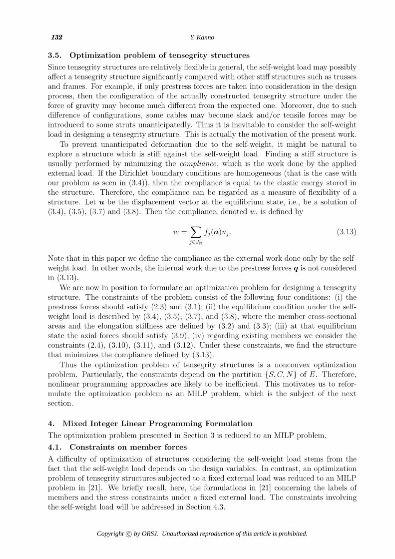
3.5. Optimization problem of tensegrity structures

Since tensegrity structures are relatively flexible in general, the self-weight load may possiblyaffect a tensegrity structure significantly compared with other stiff structures such as trussesand frames. For example, if only prestress forces are taken into consideration in the designprocess, then the configuration of the actually constructed tensegrity structure under theforce of gravity may become much different from the expected one. Moreover, due to suchdifference of configurations, some cables may become slack and/or tensile forces may beintroduced to some struts unanticipatedly. Thus it is inevitable to consider the self-weightload in designing a tensegrity structure. This is actually the motivation of the present work.

To prevent unanticipated deformation due to the self-weight, it might be natural toexplore a structure which is stiff against the self-weight load. Finding a stiff structure isusually performed by minimizing the compliance, which is the work done by the appliedexternal load. If the Dirichlet boundary conditions are homogeneous (that is the case withour problem as seen in (3.4)), then the compliance is equal to the elastic energy stored inthe structure. Therefore, the compliance can be regarded as a measure of flexibility of astructure. Let u be the displacement vector at the equilibrium state, i.e., be a solution of(3.4), (3.5), (3.7) and (3.8). Then the compliance, denoted w, is defined by

w =∑j∈JN

fj(a)uj. (3.13)

Note that in this paper we define the compliance as the external work done only by the self-weight load. In other words, the internal work due to the prestress forces q is not consideredin (3.13).

We are now in position to formulate an optimization problem for designing a tensegritystructure. The constraints of the problem consist of the following four conditions: (i) theprestress forces should satisfy (2.3) and (3.1); (ii) the equilibrium condition under the self-weight load is described by (3.4), (3.5), (3.7), and (3.8), where the member cross-sectionalareas and the elongation stiffness are defined by (3.2) and (3.3); (iii) at that equilibriumstate the axial forces should satisfy (3.9); (iv) regarding existing members we consider theconstraints (2.4), (3.10), (3.11), and (3.12). Under these constraints, we find the structurethat minimizes the compliance defined by (3.13).

Thus the optimization problem of tensegrity structures is a nonconvex optimizationproblem. Particularly, the constraints depend on the partition {S,C,N} of E. Therefore,nonlinear programming approaches are likely to be inefficient. This motivates us to refor-mulate the optimization problem as an MILP problem, which is the subject of the nextsection.

4. Mixed Integer Linear Programming Formulation

The optimization problem presented in Section 3 is reduced to an MILP problem.

4.1. Constraints on member forces

A difficulty of optimization of structures considering the self-weight load stems from thefact that the self-weight load depends on the design variables. In contrast, an optimizationproblem of tensegrity structures subjected to a fixed external load was reduced to an MILPproblem in [21]. We briefly recall, here, the formulations in [21] concerning the labels ofmembers and the stress constraints under a fixed external load. The constraints involvingthe self-weight load will be addressed in Section 4.3.



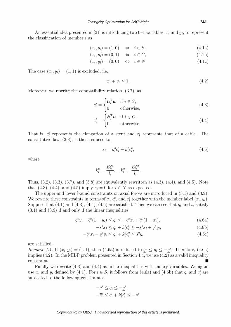
An essential idea presented in [21] is introducing two 0–1 variables, xi and yi, to representthe classification of member i as

(xi, yi) = (1, 0) ⇔ i ∈ S, (4.1a)

(xi, yi) = (0, 1) ⇔ i ∈ C, (4.1b)

(xi, yi) = (0, 0) ⇔ i ∈ N. (4.1c)

The case (xi, yi) = (1, 1) is excluded, i.e.,

xi + yi ≤ 1. (4.2)

Moreover, we rewrite the compatibility relation, (3.7), as

csi =

{hT

i u if i ∈ S,

0 otherwise,(4.3)

cci =

{hT

i u if i ∈ C,

0 otherwise.(4.4)

That is, csi represents the elongation of a strut and cci represents that of a cable. Theconstitutive law, (3.8), is then reduced to

si = ksic

si + kc

i cci , (4.5)

where

ksi =

Eξs

li, kc

i =Eξc

li.

Thus, (3.2), (3.3), (3.7), and (3.8) are equivalently rewritten as (4.3), (4.4), and (4.5). Notethat (4.3), (4.4), and (4.5) imply si = 0 for i ∈ N as expected.

The upper and lower bound constraints on axial forces are introduced in (3.1) and (3.9).We rewrite these constraints in terms of qi, c

si, and cci together with the member label (xi, yi).

Suppose that (4.1) and (4.3), (4.4), (4.5) are satisfied. Then we can see that qi and si satisfy(3.1) and (3.9) if and only if the linear inequalities

qcyi − qs(1− yi) ≤ qi ≤ −qsxi + qc(1− xi), (4.6a)

−ssxi ≤ qi + ksic

si ≤ −ssxi + qcyi, (4.6b)

−qsxi + scyi ≤ qi + kci c

ci ≤ scyi (4.6c)

are satisfied.Remark 4.1. If (xi, yi) = (1, 1), then (4.6a) is reduced to qc ≤ qi ≤ −qs. Therefore, (4.6a)implies (4.2). In the MILP problem presented in Section 4.4, we use (4.2) as a valid inequalityconstraint. ■

Finally we rewrite (4.3) and (4.4) as linear inequalities with binary variables. We againuse xi and yi defined by (4.1). For i ∈ S, it follows from (4.6a) and (4.6b) that qi and csi aresubjected to the following constraints:

−qs ≤ qi ≤ −qs,

−ss ≤ qi + ksic

si ≤ −ss.


134 Y. Kanno

These inequalities imply

qs − ss ≤ ksic

si ≤ qs − ss.

Therefore, (4.3) can be rewritten as

(qs − ss)xi ≤ ksic

si ≤ (qs − ss)xi, (4.8a)

M(1− xi) ≥ |csi − hTi u|, (4.8b)

where M ≫ 0 is a sufficiently large constant. Similarly, (4.4) can be rewritten as

(sc − qc)yi ≤ kci c

ci ≤ (sc − qc)yi, (4.9a)

M(1− yi) ≥ |cci − hTi u|. (4.9b)

4.2. Constraints on member labels

In Section 4.1 we have introduced variables (xi, yi) ∈ {0, 1}2 by (4.1) to formulate theconstraints concerning the equilibrium state under the specified external load. As the otherconstraints in terms of xi and yi, we here investigate the constraints on the numbers ofstruts and cables.

We first consider the discontinuity condition of struts, (2.4). This constraint can bewritten in terms of xi (i ∈ E) as ∑

i∈E(vp)

xi ≤ 1, ∀vp ∈ V. (4.10)

The lower bound constraint on the total number of struts was given by (3.10), which isreduced to ∑

i∈E

xi ≥ ns. (4.11)

The relation between the number of struts and that of cables was given by (3.11). Thisconstraint can be written as ∑

i∈E

(5xi − yi) = nd + 6. (4.12)

Constraint (3.12) was introduced to prevent two close members from existing together. Thisconstraint can be written in terms of xi and yi as

xi + xi′ + yi + yi′ ≤ 1, ∀(i, i′) ∈ Pcross. (4.13)

4.3. Compliance under self-weight load

We here discuss the compliance constraint under the self-weight load in the frameworkof MILP. In the force-balance equation, (3.5), the self-weight load is denoted by f(a).For simplicity, the gravity forces acting on cables are neglected, because in many real-lifetensegrity structures struts are much heavier than cables. Hence, f(a) is the sum of gravityforces acting on struts. Since the member cross-sectional area, ai, is given by (3.2), f(a)can be written as

f(a) =∑i∈E

xiξsf (i), (4.14)



Figure 3: An initial structure with three layers

where f (i) is the gravity force vector of a unit cross-sectional area of member i.

The compliance, w, is then given by (3.13) with fj(a) in (4.14). Define extra variableswi (i ∈ E) by

wi =

∑j∈JN

f(i)j uj if i ∈ S,

0 otherwise.

(4.15)

Then (3.13) is rewritten as

w =∑i∈E

wi. (4.16)

On the other hand, by using xi, (4.15) is rewritten as

Mxi ≥ |wi|, (4.17a)

M(1− xi) ≥∣∣∣wi −

∑j∈JN

f(i)j uj

∣∣∣, (4.17b)

where M is a sufficiently large constant. Thus, minimizing the compliance of a tensegritystructure is realized by minimizing w in (4.16) under constraint (4.17).

4.4. MILP formulation

We are now in position to formulate an MILP problem for topology optimization of tensegritystructures. The optimization problem was defined in Section 3.5. To reformulate thisproblem, the constraints on member forces were reduced to linear inequalities in Section 4.1by introducing 0–1 variables, xi and yi. Section 4.2 dealt with the constraints regarding thenumbers of struts and cables. In Section 4.3, the compliance constraint under the self-weightload was expressed by using linear inequalities including xi.


136 Y. Kanno

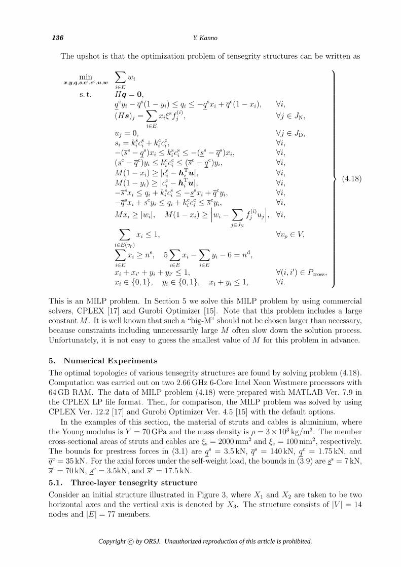
The upshot is that the optimization problem of tensegrity structures can be written as

minx,y,q,s,cs,cc,u,w

∑i∈E

wi

s. t. Hq = 0,qcyi − qs(1− yi) ≤ qi ≤ −qsxi + qc(1− xi), ∀i,(Hs)j =

∑i∈E

xiξsf

(i)j , ∀j ∈ JN,

uj = 0, ∀j ∈ JD,si = ks

icsi + kc

i cci , ∀i,

−(ss − qs)xi ≤ ksic

si ≤ −(ss − qs)xi, ∀i,

(sc − qc)yi ≤ kci c

ci ≤ (sc − qc)yi, ∀i,

M(1− xi) ≥ |csi − hTi u|, ∀i,

M(1− yi) ≥ |cci − hTi u|, ∀i,

−ssxi ≤ qi + ksic

si ≤ −ssxi + qcyi, ∀i,

−qsxi + scyi ≤ qi + kci c

ci ≤ scyi, ∀i,

Mxi ≥ |wi|, M(1− xi) ≥∣∣∣wi −

∑j∈JN

f(i)j uj

∣∣∣, ∀i,∑i∈E(vp)

xi ≤ 1, ∀vp ∈ V,∑i∈E

xi ≥ ns, 5∑i∈E

xi −∑i∈E

yi − 6 = nd,

xi + xi′ + yi + yi′ ≤ 1, ∀(i, i′) ∈ Pcross,xi ∈ {0, 1}, yi ∈ {0, 1}, xi + yi ≤ 1, ∀i.

(4.18)

This is an MILP problem. In Section 5 we solve this MILP problem by using commercialsolvers, CPLEX [17] and Gurobi Optimizer [15]. Note that this problem includes a largeconstantM . It is well known that such a “big-M” should not be chosen larger than necessary,because constraints including unnecessarily large M often slow down the solution process.Unfortunately, it is not easy to guess the smallest value of M for this problem in advance.

5. Numerical Experiments

The optimal topologies of various tensegrity structures are found by solving problem (4.18).Computation was carried out on two 2.66GHz 6-Core Intel Xeon Westmere processors with64GB RAM. The data of MILP problem (4.18) were prepared with MATLAB Ver. 7.9 inthe CPLEX LP file format. Then, for comparison, the MILP problem was solved by usingCPLEX Ver. 12.2 [17] and Gurobi Optimizer Ver. 4.5 [15] with the default options.

In the examples of this section, the material of struts and cables is aluminium, wherethe Young modulus is Y = 70GPa and the mass density is ρ = 3× 103 kg/m3. The membercross-sectional areas of struts and cables are ξs = 2000mm2 and ξc = 100mm2, respectively.The bounds for prestress forces in (3.1) are qs = 3.5 kN, qs = 140 kN, qc = 1.75 kN, andqc = 35 kN. For the axial forces under the self-weight load, the bounds in (3.9) are ss = 7kN,ss = 70 kN, sc = 3.5kN, and sc = 17.5 kN.

5.1. Three-layer tensegrity structure

Consider an initial structure illustrated in Figure 3, where X1 and X2 are taken to be twohorizontal axes and the vertical axis is denoted by X3. The structure consists of |V | = 14nodes and |E| = 77 members.



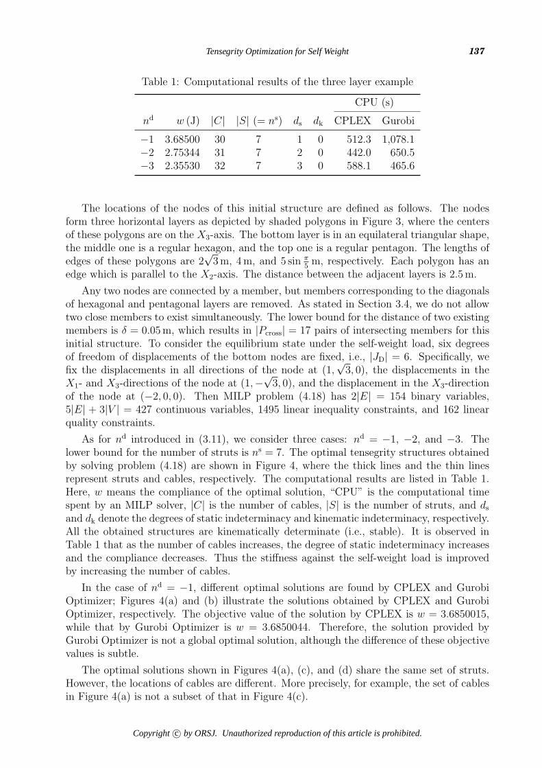
Table 1: Computational results of the three layer example

CPU (s)

nd w (J) |C| |S| (= ns) ds dk CPLEX Gurobi

−1 3.68500 30 7 1 0 512.3 1,078.1−2 2.75344 31 7 2 0 442.0 650.5−3 2.35530 32 7 3 0 588.1 465.6

The locations of the nodes of this initial structure are defined as follows. The nodesform three horizontal layers as depicted by shaded polygons in Figure 3, where the centersof these polygons are on the X3-axis. The bottom layer is in an equilateral triangular shape,the middle one is a regular hexagon, and the top one is a regular pentagon. The lengths ofedges of these polygons are 2

√3m, 4m, and 5 sin π

5m, respectively. Each polygon has an

edge which is parallel to the X2-axis. The distance between the adjacent layers is 2.5m.

Any two nodes are connected by a member, but members corresponding to the diagonalsof hexagonal and pentagonal layers are removed. As stated in Section 3.4, we do not allowtwo close members to exist simultaneously. The lower bound for the distance of two existingmembers is δ = 0.05m, which results in |Pcross| = 17 pairs of intersecting members for thisinitial structure. To consider the equilibrium state under the self-weight load, six degreesof freedom of displacements of the bottom nodes are fixed, i.e., |JD| = 6. Specifically, wefix the displacements in all directions of the node at (1,

√3, 0), the displacements in the

X1- and X3-directions of the node at (1,−√3, 0), and the displacement in the X3-direction

of the node at (−2, 0, 0). Then MILP problem (4.18) has 2|E| = 154 binary variables,5|E| + 3|V | = 427 continuous variables, 1495 linear inequality constraints, and 162 linearquality constraints.

As for nd introduced in (3.11), we consider three cases: nd = −1, −2, and −3. Thelower bound for the number of struts is ns = 7. The optimal tensegrity structures obtainedby solving problem (4.18) are shown in Figure 4, where the thick lines and the thin linesrepresent struts and cables, respectively. The computational results are listed in Table 1.Here, w means the compliance of the optimal solution, “CPU” is the computational timespent by an MILP solver, |C| is the number of cables, |S| is the number of struts, and dsand dk denote the degrees of static indeterminacy and kinematic indeterminacy, respectively.All the obtained structures are kinematically determinate (i.e., stable). It is observed inTable 1 that as the number of cables increases, the degree of static indeterminacy increasesand the compliance decreases. Thus the stiffness against the self-weight load is improvedby increasing the number of cables.

In the case of nd = −1, different optimal solutions are found by CPLEX and GurobiOptimizer; Figures 4(a) and (b) illustrate the solutions obtained by CPLEX and GurobiOptimizer, respectively. The objective value of the solution by CPLEX is w = 3.6850015,while that by Gurobi Optimizer is w = 3.6850044. Therefore, the solution provided byGurobi Optimizer is not a global optimal solution, although the difference of these objectivevalues is subtle.

The optimal solutions shown in Figures 4(a), (c), and (d) share the same set of struts.However, the locations of cables are different. More precisely, for example, the set of cablesin Figure 4(a) is not a subset of that in Figure 4(c).


138 Y. Kanno

(a) (b)

(c) (d)

Figure 4: Optimal solutions obtained from the three-layer initial structure in Figure 3.(a) nd = −1 by CPLEX; (b) nd = −1 by Gurobi Optimizer; (c) nd = −2; (d) nd = −3

5.2. Cantilevered tensegrity structure

We next consider an initial structure illustrated in Figure 5. The structure consists of|V | = 14 nodes and |E| = 82 members. The number of pairs of intersecting members (withthreshold δ = 0.05m) is |Pcross| = 23.

The locations of the nodes of this initial structure are defined as follows. The nodes formfour vertical layers, which are two equilateral triangles and two squares as shown in Figure 5.We call these layers L1, L2, L3, and L4, where the leftmost one is L1 and the rightmost oneis L4. The lengths of edges of L1 and L4 are

√3m, while those of L2 and L3 are 1.25

√2m.

All the layers are parallel to the X2X3-plane and their centers are on the X1-axis. Moreover,each of L1, L3, and L4 has an edge which is parallel to the X2-axis. Then L2 is rotated fromL3 counter-clockwise around the X1-axis with the angle π/12. The X1-coordinates of thenodes of L1, L2, L3, and L4 are 0m, 4.25m, 4.75m, and 9m, respectively.

Any two nodes of the initial structure are connected by a member, but members con-necting the pair L1 and L4 are removed to avoid presence of too long members. To considerthe equilibrium state under the self-weight load, all the nodes of L1 are fixed. Therefore,|JD| = 9 and |JN| = 33. Such a structure anchored at only one end on a wall is called acantilever . MILP problem (4.18) includes 2|E| = 164 binary variables, 5|E| + 3|V | = 452



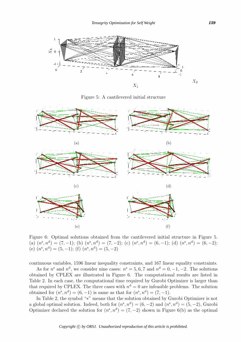
Figure 5: A cantilevered initial structure

(a) (b)

(c) (d)

(e) (f)

Figure 6: Optimal solutions obtained from the cantilevered initial structure in Figure 5.(a) (ns, nd) = (7,−1); (b) (ns, nd) = (7,−2); (c) (ns, nd) = (6,−1); (d) (ns, nd) = (6,−2);(e) (ns, nd) = (5,−1); (f) (ns, nd) = (5,−2)

continuous variables, 1596 linear inequality constraints, and 167 linear equality constraints.As for ns and nd, we consider nine cases: ns = 5, 6, 7 and nd = 0,−1,−2. The solutions

obtained by CPLEX are illustrated in Figure 6. The computational results are listed inTable 2. In each case, the computational time required by Gurobi Optimizer is larger thanthat required by CPLEX. The three cases with nd = 0 are infeasible problems. The solutionobtained for (ns, nd) = (6,−1) is same as that for (ns, nd) = (7,−1).

In Table 2, the symbol “∗” means that the solution obtained by Gurobi Optimizer is nota global optimal solution. Indeed, both for (ns, nd) = (6,−2) and (ns, nd) = (5,−2), GurobiOptimizer declared the solution for (ns, nd) = (7,−2) shown in Figure 6(b) as the optimal


140 Y. Kanno

Table 2: Computational results of the cantilevered example

CPU (s)

ns nd w (J) |C| |S| ds dk CPLEX Gurobi

7 0 infeasible — — — — 89.1 417.37 −1 30.8941 30 7 1 0 93.5 1,096.97 −2 19.5696 31 7 2 0 107.9 12,521.66 0 infeasible — — — — 124.3 385.96 −1 30.8941 30 7 1 0 139.4 303.46 −2 14.6165 26 6 2 0 100.6 ∗5 0 infeasible — — — — 206.5 629.85 −1 1.0729 20 5 1 0 163.0 595.55 −2 1.0243 21 5 2 0 145.5 ∗

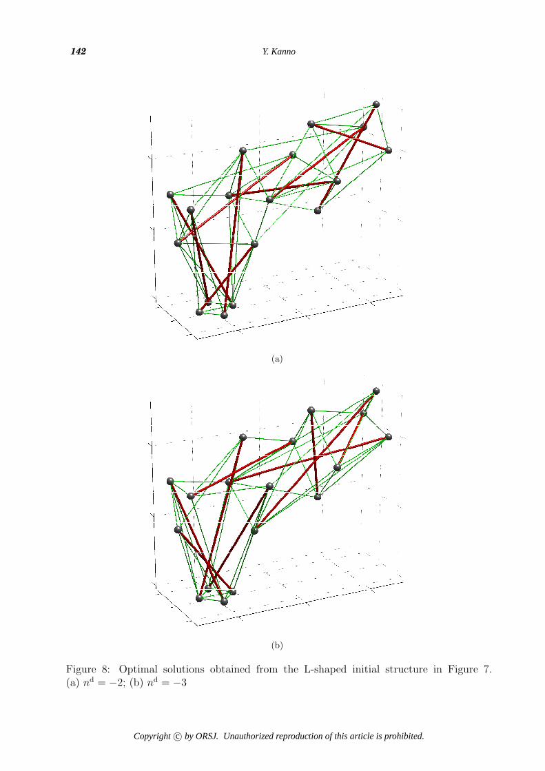
Figure 7: An L-shaped initial structure

solutions. It is evident from Table 2 that the solutions obtained by CPLEX in these twocases have smaller objective values than the solution for (ns, nd) = (7,−2).

5.3. L-shaped tensegrity structure

In this section we consider an initial structure illustrated in Figure 7. This structure consistsof |V | = 18 nodes and |E| = 116 members. The locations of the nodes are listed in Table 3.The nodes form five regular polygons, i.e., two equilateral triangles and three squares, asshown in Figure 7. We call the bottom square L1. The remaining polygons are calledL2, . . . , L5, where the leftmost triangle is L2 and the rightmost triangle is L5. Squares L1

and L3 are parallel to the X1X2-plane and the X2X3-plane, respectively. The lengths ofedges of L1 are

√2/2m, those of L2 and L5 are 3

√3/4m, and those of L3 and L4 are

5√2/4m.The members connecting the pairs {L1, L4}, {L1, L5}, and {L2, L5} are not considered.

The number of pairs of intersecting members (with threshold δ = 0.05m) is |Pcross| = 53.



Table 3: Locations of the nodes of the L-shaped initial structure in Figure 7

L1 L2 L3 L4 L5

Node 1 X1 0.5000 −0.9749 1.0000 2.8682 4.9122X2 0.0000 0.6495 1.2074 0.0000 0.7244X3 0.0000 3.1993 2.6765 4.7682 4.1980

Node 2 X1 0.0000 −1.0730 1.0000 2.9772 4.9706X2 0.5000 0.0000 −0.3235 1.2500 −0.5303X3 0.0000 2.0785 1.7926 3.5229 3.8669

Node 3 X1 −0.5000 −0.9749 1.0000 3.0861 4.7527X2 0.0000 −0.6495 −1.2074 0.0000 −0.1941X3 0.0000 3.1993 3.3235 2.2777 5.1026

Node 4 X1 0.0000 1.0000 2.9772X2 −0.5000 0.3235 −1.2500X3 0.0000 4.2074 3.5229

Table 4: Computational results of the L-shaped example

CPU (s)

nd w (J) |C| |S| (= ns) ds dk CPLEX Gurobi

−1 infeasible — — — — 18,286.1 ∗∗−2 6.3504 41 9 2 0 14,459.3 ∗∗−3 9.6019 42 9 3 0 35,559.7 ∗∗

The equilibrium state under the self-weight load is considered by fixing all four nodes of L1.Hence, |JD| = 12 and |JN| = 42. The lower bound for the number of struts is ns = 9. Thenproblem (4.18) has 2|E| = 232 binary variables, 5|E| + 3|V | = 634 continuous variables,2276 linear inequality constraints, and 225 linear equality constraints.

The computational results are listed in Table 4. Here, the symbol “∗∗” means thatGurobi Optimizer does not terminate within 100,000 s. The solutions obtained by CPLEXare shown in Figure 8. It is observed that sets of struts are different between Figures 8(a)and (b).

6. Conclusions

For developing real-world innovative tensegrity structures, form-finding methods that canexplore diverse topologies are desired. In this paper we have explored a topology optimiza-tion problem of tensegrity structures subjected to self-weight loads. The presented approachprepares an initial structure with sufficiently large number of candidate members and doesnot require a topology of tensegrity structures to be known in advance. The optimizationproblem has been reduced to an MILP problem. It has been shown in numerical examplesthat various configurations of tensegrity structures can be obtained by solving this MILPproblem. The numerical experiments illustrate that, for this MILP problem, Gurobi Opti-mizer is not superior to CPLEX from viewpoints of computational efficiency and accuracy.

This paper has not addressed issues of stability of tensegrity structures. The tensegrity


142 Y. Kanno

(a)

(b)

Figure 8: Optimal solutions obtained from the L-shaped initial structure in Figure 7.(a) nd = −2; (b) nd = −3



structures obtained in Section 5 are kinematically determinate (i.e., stable), whereas manywell-known tensegrity structures are kinematically indeterminate (i.e., unstable) and stabi-lized by introducing prestress forces; see, e.g., Calladine [7], Guest [14], Hanaor and Liao[16], and Pellegrino [25]. Therefore, it remains as an important future subject to develop anumerical method that can find unstable (but prestress stable) tensegrity structures. Also,the geometrical nonlinearity has not been considered. Furthermore, the proposed formula-tion results in a large MILP problem, which might be a potential disadvantage for findingtensegrity structures consisting of a large number of members.

Acknowledgments

This work is partially supported by Grant-in-Aid for Scientific Research (C) 23560663, bythe Global COE Program “The Research and Training Center for New Development inMathematics,” and by the Aihara Project, the FIRST program from JSPS, initiated byCSTP.

References

[1] B. Adam and I.F.C. Smith: Active tensegrity: a control framework for an adaptivecivil-engineering structure. Computers and Structures, 86 (2008), 2215–2223.

[2] T.M. Atanackovic: Optimal shape of column with own weight: bi and single modaloptimization. Meccanica, 41 (2006), 173–196.

[3] A. Back and R. Connelly: Catalogue of Symmetric Tensegrities (web page).http://mathlab.cit.cornell.edu/visualization/tenseg/tenseg.html (AccessedOctober 2011).

[4] N. Bel Hadj Ali, L. Rhode-Barbarigos, A.A. Pascual Albi, and I.F.C. Smith: Designoptimization and dynamic analysis of a tensegrity-based footbridge. Engineering Struc-tures, 32 (2010), 3650–3659.

[5] S. Bereg: On characterizations of rigid graphs in the plane using spanning trees. Graphsand Combinatorics, 25 (2009), 139–144.

[6] M. Bruyneel and P. Duysinx: Note on topology optimization of continuum structuresincluding self-weight. Structural and Multidisciplinary Optimization, 29 (2005), 245–256.

[7] C.R. Calladine: Buckminster Fuller’s “tensegrity” structures and Clerk Maxwell’s rulesfor the construction of stiff frames. International Journal of Solids and Structures, 14(1978), 161–172.

[8] R. Connelly and A. Back: Mathematics and tensegrity. American Scientist, 86 (1998),142–151.

[9] R. Connelly and W. Whiteley: Second-order rigidity and prestress stability for tenseg-rity frameworks. SIAM Journal on Discrete Mathematics, 6 (1996), 453–491.

[10] S. Ehara and Y. Kanno: Topology design of tensegrity structures via mixed integerprogramming. International Journal of Solids and Structures, 47 (2010), 571–579.

[11] D.G. Emmerich: Construction de reseaux autotendants. French Patent No. 1,377,290,September 28, 1964.

[12] R.B. Fuller: Tensile-integrity structures. U.S. Patent No. 3,063,521, November 13, 1962.

[13] R.B. Fuller: Synergetics: Explorations in the Geometry of Thinking (Collier McMillian,London, 1975).


144 Y. Kanno

[14] S.D. Guest: The stiffness of tensegrity structures. IMA Journal of Applied Mathematics,76 (2011), 57–66.

[15] Gurobi Optimization, Inc.: Gurobi Optimizer Reference Manual.http://www.gurobi.com/ (2010).

[16] A. Hanaor and M.-K. Liao: Double-layer tensegrity grids: static load response. Part I:analytical study. Journal of Structural Engineering (ASCE), 117 (1991), 1660–1674.

[17] IBM ILOG: User’s Manual for CPLEX. http://www.ilog.com/ (2010).

[18] M.H. Imam: Shape optimization of umbrella-shaped concrete shells subjected to self-weight as the dominant load. Computers and Structures, 69 (1998), 513–524.

[19] T. Jordan, A. Recski, and Z. Szabadka: Rigid tensegrity labelings of graphs. EuropeanJournal of Combinatorics, 30 (2009), 1887–1895.

[20] S.H. Juan and J.M. Mirats Tur: Tensegrity frameworks: static analysis review. Mech-anism and Machine Theory, 43 (2008), 859–881.

[21] Y. Kanno: Topology optimization of tensegrity structures under compliance constraint:a mixed integer linear programming approach. Optimization and Engineering, to ap-pear.

[22] B.L. Karihaloo and S. Kanagasundaram: Optimum design of statically indeterminatebeams under multiple loads. Computers and Structures, 26 (1987), 521–538.

[23] D.-Y. Kwak, J.-H. Jeong, J.-S. Cheon, and Y.-T. Im: Optimal design of compositehood with reinforcing ribs through stiffness analysis. Composite Structures, 38 (1997),351–359.

[24] R. Motro: Tensegrity (Kogan Page Science, London, 2003).

[25] S. Pellegrino: A class of tensegrity domes. International Journal of Space Structures, 7(1992), 127–142.

[26] J. Rieffel, F. Valero-Cuevasa, and H. Lipson: Automated discovery and optimizationof large irregular tensegrity structures. Computers and Structures, 87 (2009), 368–379.

[27] G.I.N. Rozvany: Optimal plastic design: allowance for selfweight. Journal of the Engi-neering Mechanics Division (ASCE), 103 (1977), 1165–1170.

[28] G.I.N. Rozvany, H. Nakanamura, and B.T. Kuhnell: Optimal archgrids: allowancefor selfweight. Computer Methods in Applied Mechanics and Engineering, 24 (1980),287–304.

[29] G.I.N. Rozvany, K.M. Yep, T.G. Ong, and B.L. Karihaloo: Optimal design of elasticbeams under multiple design constraints. International Journal of Solids and Struc-tures, 24 (1988), 331–349.

[30] K. Snelson: Continuous tension, discontinuous compression structures. U.S. PatentNo. 3,169,611, February 16, 1965.

[31] K. Snelson: Kenneth Snelson (web page). http://www.kennethsnelson.net/ (Ac-cessed October 2011).

[32] A.M.C. So and Y. Ye: A semidefinite programming approach to tensegrity theoryand realizability of graphs. Proceedings of the 17th Annual ACM-SIAM Symposium onDiscrete Algorithms (SODA 06), 766–775, Miami (2006).

[33] C. Sultan and R. Skelton: Deployment of tensegrity structures. International Journalof Solids and Structures, 40 (2003), 4637–4657.

[34] A.G. Tibert and S. Pellegrino: Deployable tensegrity reflectors for small satellites.Journal of Spacecraft and Rockets (AIAA), 39 (2002), 701–709.



[35] A.G. Tibert and S. Pellegrino: Review of form-finding methods for tensegrity struc-tures. International Journal of Space Structures, 18 (2003), 209–223.

[36] K.Yu. Volokh, O. Vilnay, and M. Belsky: Tensegrity architecture explains linear stiff-ening and predicts softening of living cells. Journal of Biomechanics, 33 (2000), 1543–1549.

[37] S. Wandling, P. Canadas, and P. Chabrand: Towards a generalised tensegrity modeldescribing the mechanical behaviour of the cytoskeleton structure. Computer Methodsin Biomechanics and Biomedical Engineering, 6 (2003), 45–52.

[38] C.-M. Wang and G.I.N. Rozvany: On plane Prager-structures—II: nonparallel externalloads and allowance for selfweight. International Journal of Mechanical Sciences, 25(1983), 529–541.

Yoshihiro KannoDepartment of Mathematical InformaticsUniversity of Tokyo7-3-1 Hongo, Tokyo 113-8656, JapanE-mail: [email protected]


Documents

TOPOLOGY OPTIMIZATION OF TENSEGRITY …archive/pdf/e_mag/Vol.55_02_125.pdf · cables of a tensegrity structure. Finding new topologies of ... and cell cytoskeleton models in biomechanics