Embed Size (px)
Citation preview

Yohanes E. Riyanto EC 3322 (Industrial Organization I) 1
EC 3322 Semester I – 2008/2009
Topic 9: Product Differentiation
Yohanes E. Riyanto EC 3322 (Industrial Organization I) 2
Introduction Firms produce similar but not identical products (differentiated) in
many different ways.
Horizontally
Goods of similar quality targeted at consumers of different types/ preference/ taste/ location
How is variety determined? How does competition influence the equilibrium variety.
Vertically
Consumers agree that there are quality differences.
They differ in willingness to pay for quality.
What determine the quality of goods?
Yohanes E. Riyanto EC 3322 (Industrial Organization I) 3
Introduction … Modeling horizontal product differentiation:
Representative Consumer Model
Firms producing differentiated goods compete equally for all consumers.
Demand is continuous the usual (inverse) demand function a small change in any one firm’s quantity (or price) a small change in demand.
Spatial/ Location/ Address Model
Consumers may prefer products with certain characteristics (taste, location, sugar contents, etc) are willing to pay premium for the preferred products.
Demand maybe independent (not close substitutes) or highly dependent (close substitutes)
Yohanes E. Riyanto EC 3322 (Industrial Organization I) 4
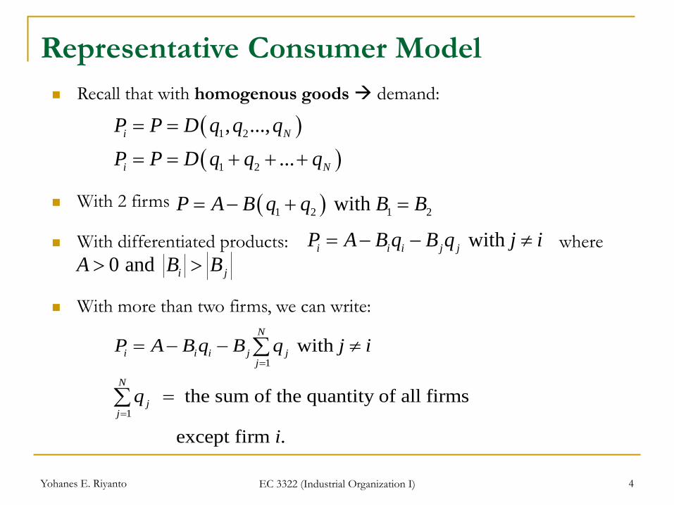
Representative Consumer Model Recall that with homogenous goods demand:
With 2 firms
With differentiated products: where
With more than two firms, we can write:
( )( )
1 2
1 2
, ...,...
i N
i N
P P D q q qP P D q q q
= =
= = + + +
( )1 2 1 2 with P A B q q B B= − + =
with i i i j jP A B q B q j i= − − ≠0 and i jA B B> >
1
1
with
the sum of the quantity of all firms
except firm .
N
i i i j jj
N
jj
P A B q B q j i
q
i
=
=
= − − ≠
=
∑
∑
Yohanes E. Riyanto EC 3322 (Industrial Organization I) 5
Representative Consumer Model…
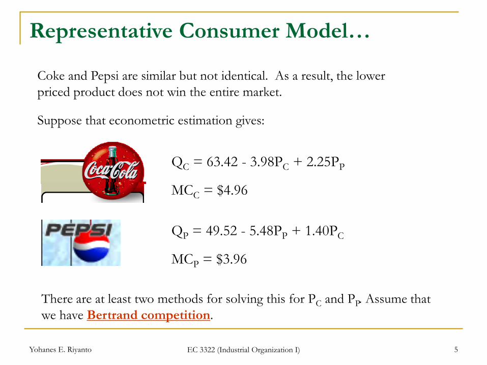
QC = 63.42 - 3.98PC + 2.25PP
QP = 49.52 - 5.48PP + 1.40PC
MCC = $4.96
MCP = $3.96
There are at least two methods for solving this for PC and PP. Assume that we have Bertrand competition.
Coke and Pepsi are similar but not identical. As a result, the lower priced product does not win the entire market.
Suppose that econometric estimation gives:
Yohanes E. Riyanto EC 3322 (Industrial Organization I) 6
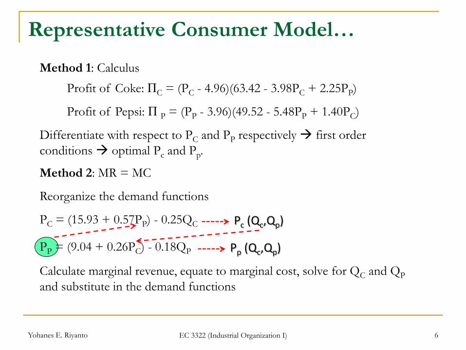
Method 1: Calculus Profit of Coke: ΠC = (PC - 4.96)(63.42 - 3.98PC + 2.25PP)
Profit of Pepsi: Π P = (PP - 3.96)(49.52 - 5.48PP + 1.40PC)
Differentiate with respect to PC and PP respectively first order conditions optimal Pc and Pp.
Method 2: MR = MC
Reorganize the demand functions
PC = (15.93 + 0.57PP) - 0.25QC
PP = (9.04 + 0.26PC) - 0.18QP
Calculate marginal revenue, equate to marginal cost, solve for QC and QP and substitute in the demand functions
Representative Consumer Model…
Pc (Qc,Qp)
Pp (Qc,Qp)

Yohanes E. Riyanto EC 3322 (Industrial Organization I) 7
Both methods give the best response functions:
PC = 10.44 + 0.2826PP
PP = 6.49 + 0.1277PC
PC
PP RC
$10.44
RP
Note that these are upward
sloping
The Bertrand equilibrium is
at their intersection
B
$12.72
$8.11
$6.49
These can be solved for the equilibrium prices as indicated
The equilibrium prices are each greater than marginal cost
Representative Consumer Model…
Yohanes E. Riyanto EC 3322 (Industrial Organization I) 8
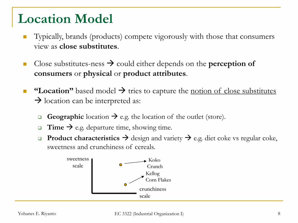
Location Model Typically, brands (products) compete vigorously with those that consumers
view as close substitutes.
Close substitutes-ness could either depends on the perception of consumers or physical or product attributes.
“Location” based model tries to capture the notion of close substitutes location can be interpreted as:
Geographic location e.g. the location of the outlet (store). Time e.g. departure time, showing time. Product characteristics design and variety e.g. diet coke vs regular coke,
sweetness and crunchiness of cereals. sweetness
scale
crunchiness scale
Kellog Corn Flakes
Koko Crunch

Yohanes E. Riyanto EC 3322 (Industrial Organization I) 9
Location Model… Based on Hotelling (1929) Hotelling’s Linear Street Model.
Imagine e.g. a long stretch of beach with ice cream shops (sellers) along it.
The model discusses the “location” and “pricing behavior” of firms.
Basic Setup:
N-consumers are uniformly distributed along this linear street thus in any block of the street there are an equal number of consumers.
Consumers are identical except for location and each of them are considering buying exactly one unit of product as long as the price paid + other costs are lower than the value derived from consuming the product (V).
As a benchmark, consider for the time being the case of a monopoly seller operates only 1 store it is reasonable to expect that it is located in the middle.
Consumers incur “transportation” costs per unit of distance (e.g. mile) traveled, t.
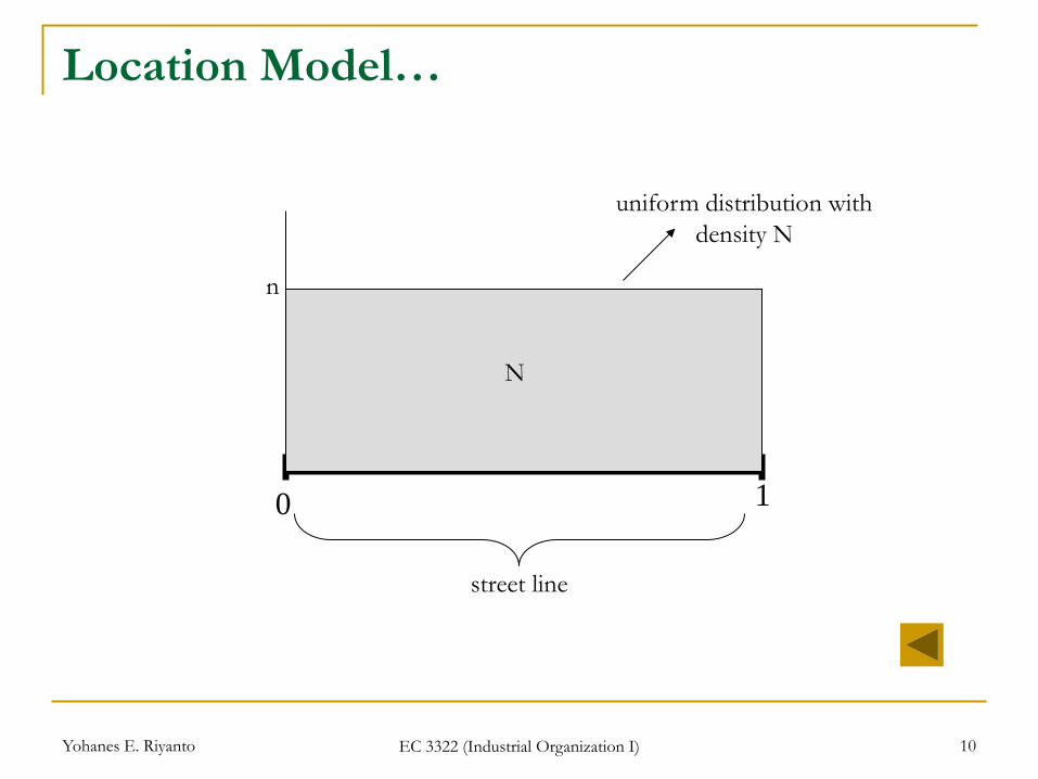
Yohanes E. Riyanto EC 3322 (Industrial Organization I) 10
10
n
N
uniform distribution with density N
Location Model…
street line
Yohanes E. Riyanto EC 3322 (Industrial Organization I) 11
Hotelling Model…
z = 0 z = 1
Shop 1
t
x1
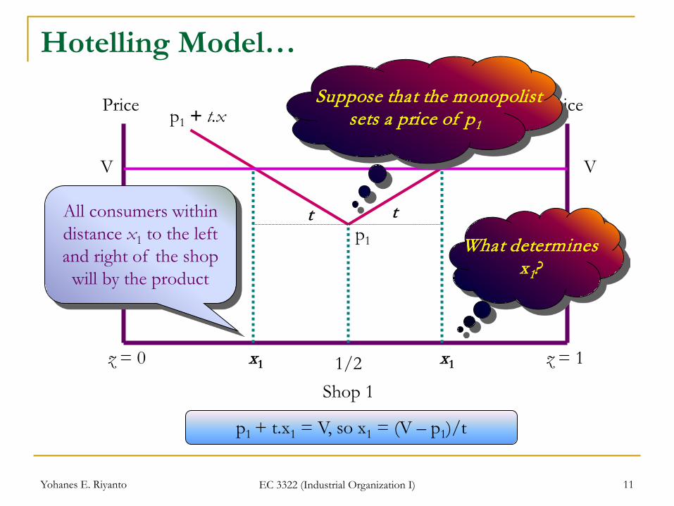
Price Price
All consumers within distance x1 to the left and right of the shop
will by the product
1/2
V V
p1 t
x1
p1 + t.x p1 + t.x
p1 + t.x1 = V, so x1 = (V – p1)/t
What determines x1?
Suppose that the monopolist sets a price of p1
Yohanes E. Riyanto EC 3322 (Industrial Organization I) 12
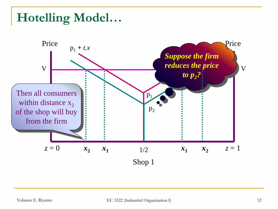
z = 0 z = 1
Shop 1
x1
Price Price
1/2
V V
p1
x1
p1 + t.x p1 + t.x Suppose the firm reduces the price
to p2?
p2
x2 x2
Then all consumers within distance x2
of the shop will buy from the firm
Hotelling Model…
Yohanes E. Riyanto EC 3322 (Industrial Organization I) 13
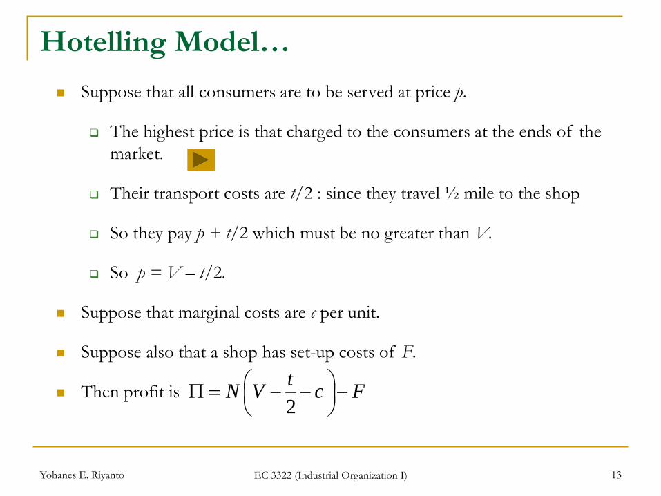
Suppose that all consumers are to be served at price p.
The highest price is that charged to the consumers at the ends of the market.
Their transport costs are t/2 : since they travel ½ mile to the shop
So they pay p + t/2 which must be no greater than V.
So p = V – t/2.
Suppose that marginal costs are c per unit.
Suppose also that a shop has set-up costs of F.
Then profit is
Hotelling Model…
2tN V c F Π = − − −
Yohanes E. Riyanto EC 3322 (Industrial Organization I) 14
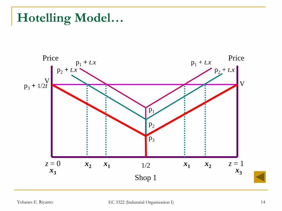
z = 0 z = 1
Shop 1
x1
Price Price
1/2
V V
p1
x1
p1 + t.x p1 + t.x
p2
x2 x2
Hotelling Model…
x3 x3
p3
p2 + t.x p2 + t.x
p3 + 1/2t
Yohanes E. Riyanto EC 3322 (Industrial Organization I) 15
What if there are two shops and these two shops are competitors? Consumers buy from the shop who can offer the lower full price
(product price + transportation cost). Suppose that location of these two shops are fixed at both ends
of the street, and they compete only in price. How large is the demand obtained by each firm and what prices are
they going to charge?
Hotelling Model…
Yohanes E. Riyanto EC 3322 (Industrial Organization I) 16
Hotelling Model…
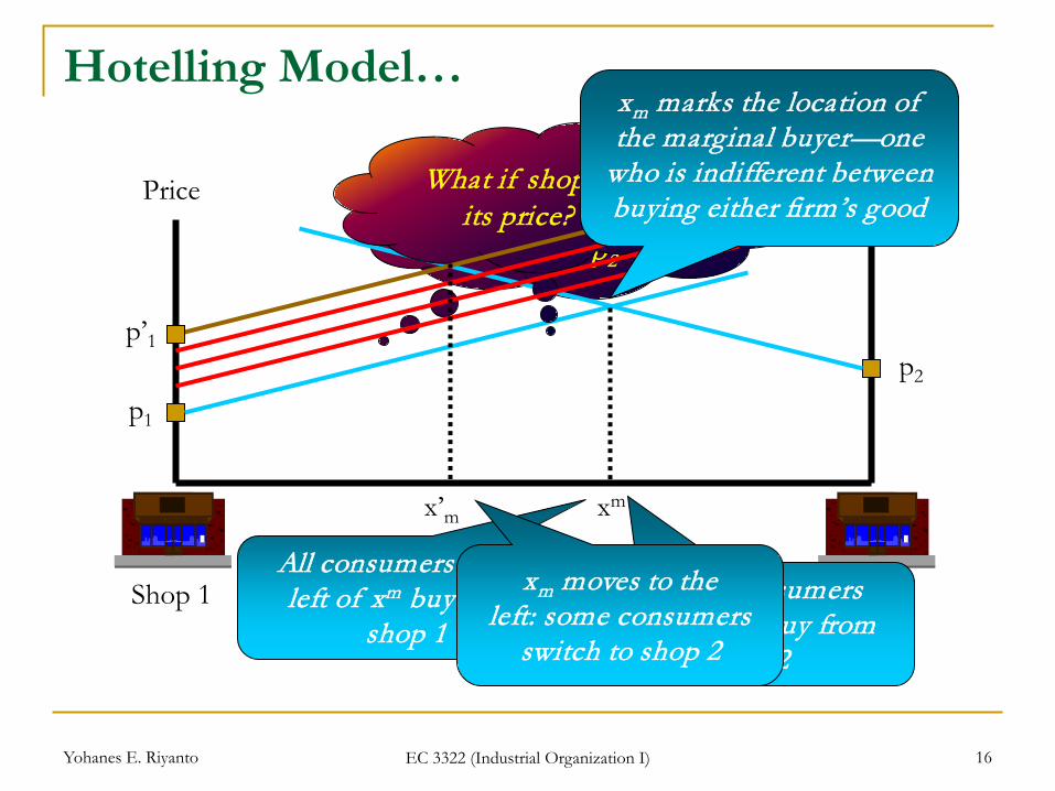
Shop 1 Shop 2
Assume that shop 1 sets price p1 and shop 2 sets
price p2
Price Price
p1 p2
xm
All consumers to the left of xm buy from
shop 1 And all consumers
to the right buy from shop 2
What if shop 1 raises its price?
p’1
x’m
xm moves to the left: some consumers
switch to shop 2
xm marks the location of the marginal buyer—one
who is indifferent between buying either firm’s good
Yohanes E. Riyanto EC 3322 (Industrial Organization I) 17
Hotelling Model…
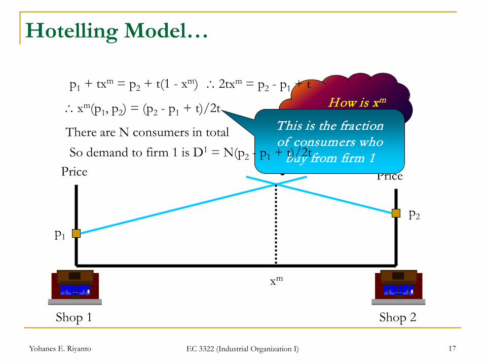
Shop 1 Shop 2
Price Price
p1 p2
xm
How is xm determined?
p1 + txm = p2 + t(1 - xm) ∴2txm = p2 - p1 + t
∴xm(p1, p2) = (p2 - p1 + t)/2t This is the fraction of consumers who
buy from firm 1 So demand to firm 1 is D1 = N(p2 - p1 + t)/2t There are N consumers in total

Yohanes E. Riyanto EC 3322 (Industrial Organization I) 18
Hotelling Model…
Profit to firm 1 is π1 = (p1 - c)D1 = N(p1 - c)(p2 - p1 + t)/2t
π1 = N(p2p1 - p12 + tp1 + cp1 - cp2 -ct)/2t
Differentiate with respect to p1
∂π1/ ∂p1 = N 2t
(p2 - 2p1 + t + c) = 0
Solve this for p1
p*1 = (p2 + t + c)/2
What about firm 2? By symmetry, it has a similar best response function.
This is the best response function
for firm 1
p*2 = (p1 + t + c)/2
This is the best response function for firm 2
Yohanes E. Riyanto EC 3322 (Industrial Organization I) 19
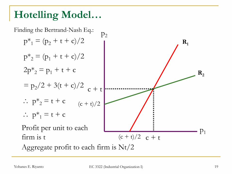
Hotelling Model…
p*1 = (p2 + t + c)/2 p2
p1
R1
p*2 = (p1 + t + c)/2
R2
(c + t)/2
(c + t)/2
2p*2 = p1 + t + c
= p2/2 + 3(t + c)/2
∴ p*2 = t + c c + t
∴ p*1 = t + c
c + t Profit per unit to each firm is t Aggregate profit to each firm is Nt/2
Finding the Bertrand-Nash Eq.:
Yohanes E. Riyanto EC 3322 (Industrial Organization I) 20
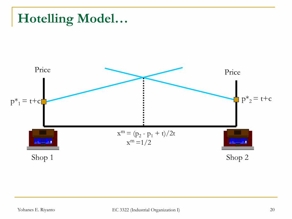
Shop 1 Shop 2
Price Price
p*1 = t+c p*2 = t+c
xm = (p2 - p1 + t)/2t
Hotelling Model…
xm =1/2
Yohanes E. Riyanto EC 3322 (Industrial Organization I) 21
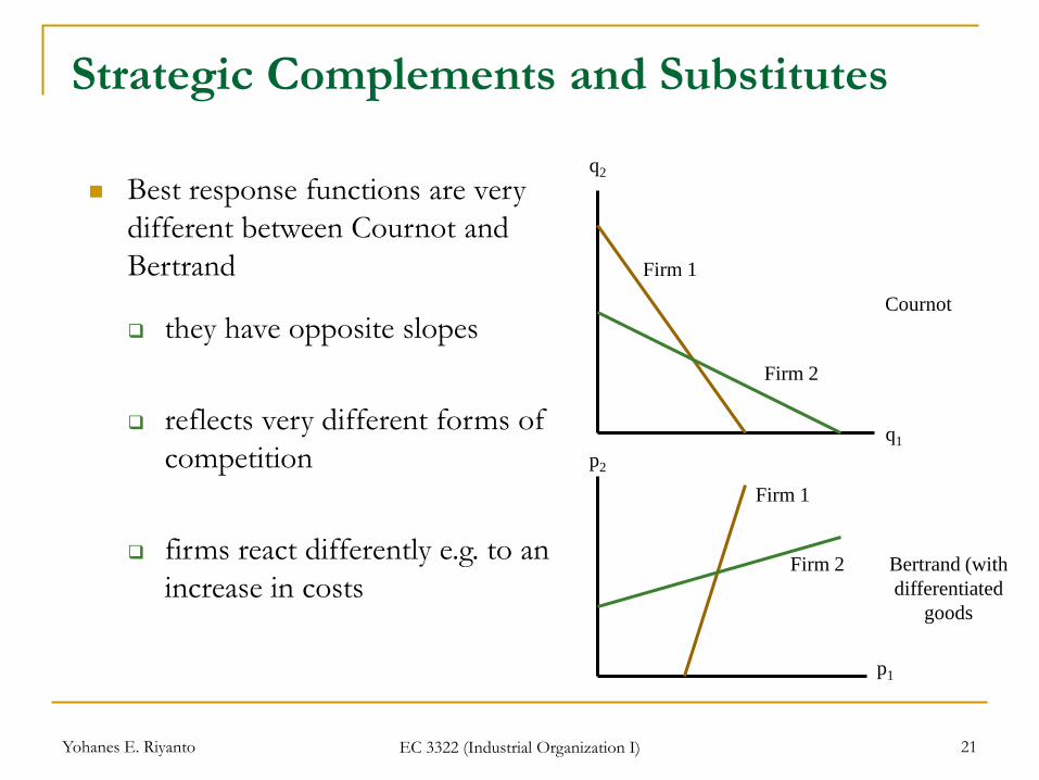
Strategic Complements and Substitutes
Best response functions are very different between Cournot and Bertrand
q2
q1 p2
p1
Firm 1
Firm 1
Firm 2
Firm 2
Cournot
Bertrand (with differentiated
goods
they have opposite slopes
reflects very different forms of competition
firms react differently e.g. to an increase in costs
Yohanes E. Riyanto EC 3322 (Industrial Organization I) 22
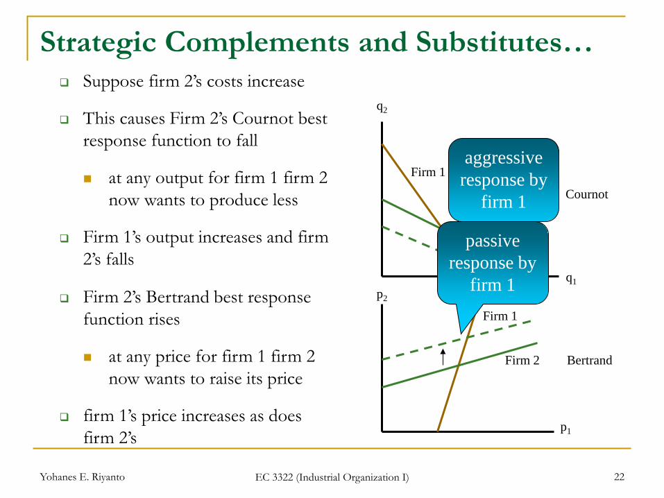
Strategic Complements and Substitutes…
p2
p1
Firm 1
Firm 2
q2
q1
Firm 1
Firm 2
Cournot
Bertrand
Suppose firm 2’s costs increase
This causes Firm 2’s Cournot best response function to fall
at any output for firm 1 firm 2 now wants to produce less
Firm 1’s output increases and firm 2’s falls
aggressive response by
firm 1
Firm 2’s Bertrand best response function rises
at any price for firm 1 firm 2 now wants to raise its price
firm 1’s price increases as does firm 2’s
passive response by
firm 1
Yohanes E. Riyanto EC 3322 (Industrial Organization I) 23
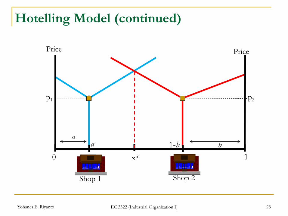
Hotelling Model (continued)
xm 0 1
a b
Shop 2
1-b
Shop 1
a
Price Price
p1 p2
Yohanes E. Riyanto EC 3322 (Industrial Organization I) 24
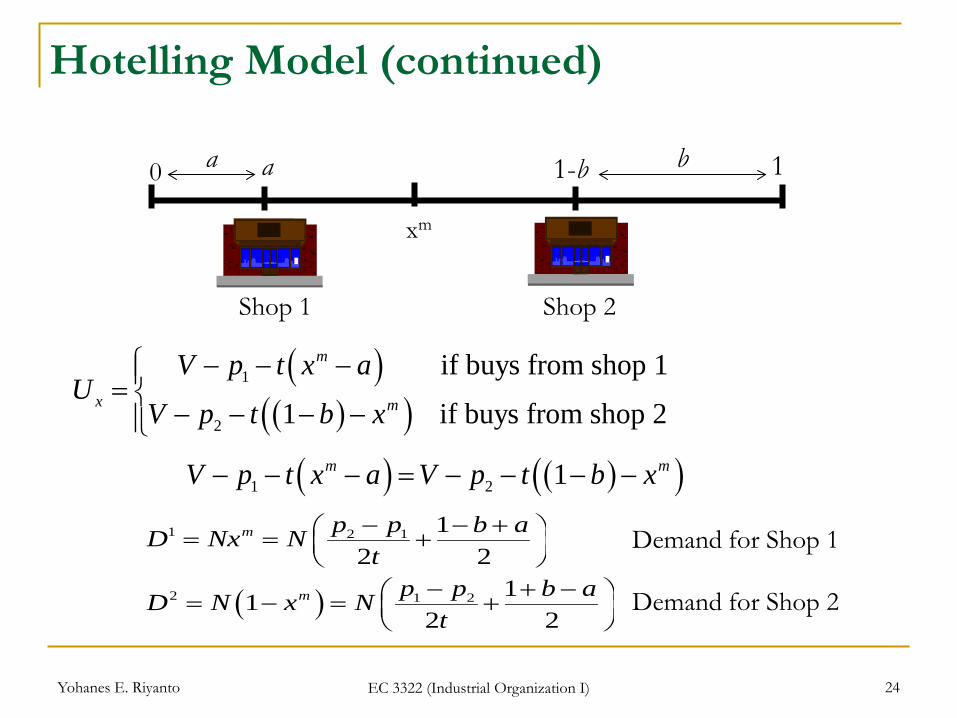
Hotelling Model (continued)
0 1
xm
a b
Shop 2
1-b
Shop 1
a
( )( )( )
1
2
if buys from shop 1 1 if buys from shop 2
m
x m
V p t x aU
V p t b x
− − −= − − − −
( ) ( )( )1 2 1m mV p t x a V p t b x− − − = − − − −
1 2 1 12 2
m p p b aD Nx Nt
− − + = = +
Demand for Shop 1
( )2 1 2 112 2
m p p b aD N x Nt
− + − = − = +
Demand for Shop 2
Yohanes E. Riyanto EC 3322 (Industrial Organization I) 25
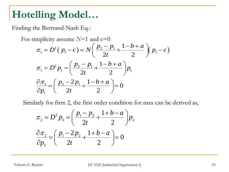
Hotelling Model… Finding the Bertrand-Nash Eq.:
( ) ( )1 2 11 1 1
1 2 11 1 1
1 2 1
1
12 2
12 2
2 1 02 2
p p b aD p c N p ct
p p b aD p pt
p p b ap t
π
π
π
− − + = − = + −
− − + = = +
∂ − − + = + = ∂
For simplicity assume N=1 and c=0
Similarly for firm 2, the first order condition for max can be derived as,
2 1 22 2 2
2 1 2
2
12 2
2 1 02 2
π
π
− + − = = +
∂ − + − = + = ∂
p p b aD p pt
p p b ap t
Yohanes E. Riyanto EC 3322 (Industrial Organization I) 26
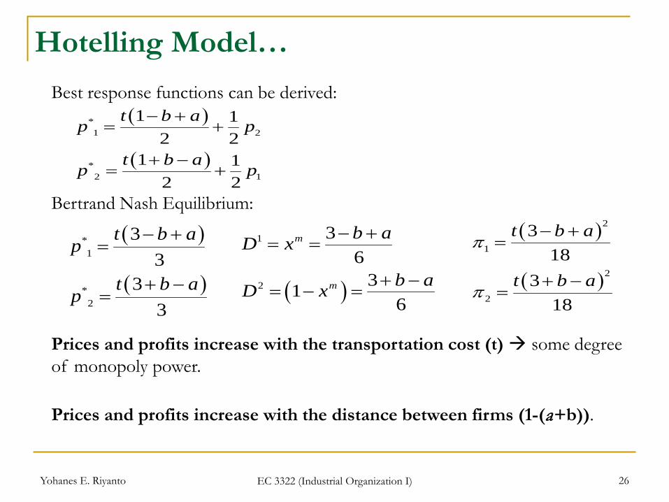
Hotelling Model… Best response functions can be derived:
( )
( )
*1 2
*2 1
1 12 2
1 12 2
t b ap p
t b ap p
− += +
+ −= +
Bertrand Nash Equilibrium:
( )
( )
*1
*2
33
33
t b ap
t b ap
− +=
+ −= ( )
1
2
36
316
m
m
b aD x
b aD x
− += =
+ −= − =
( )
( )
2
1
2
2
318
318
t b a
t b a
π
π
− +=
+ −=
Prices and profits increase with the transportation cost (t) some degree of monopoly power.
Prices and profits increase with the distance between firms (1-(a+b)).
Yohanes E. Riyanto EC 3322 (Industrial Organization I) 27
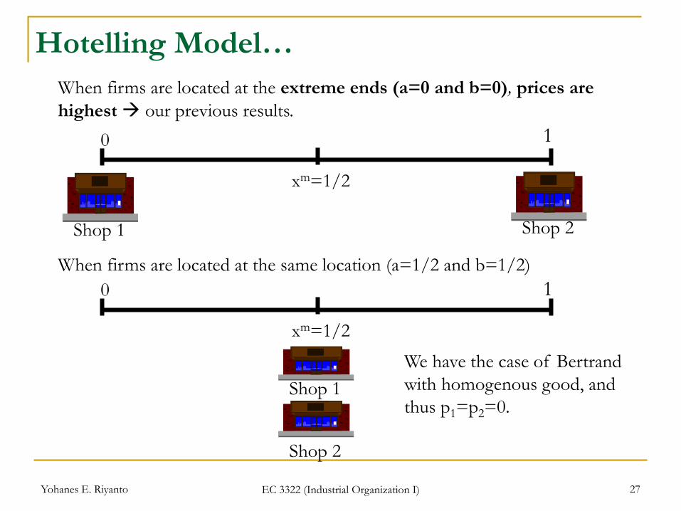
When firms are located at the extreme ends (a=0 and b=0), prices are highest our previous results.
Hotelling Model…
When firms are located at the same location (a=1/2 and b=1/2)
Shop 1 Shop 2
xm=1/2
0 1
Shop 1
Shop 2
xm=1/2
0 1
We have the case of Bertrand with homogenous good, and thus p1=p2=0.

Yohanes E. Riyanto EC 3322 (Industrial Organization I) 28
Hotelling Model… Two final points on this analysis
t is a measure of transport costs
it is also a measure of the value consumers place on getting their most preferred variety
when t is large competition is softened
and profit is increased
when t is small competition is tougher
and profit is decreased
Locations have been taken as fixed what happen when firms also choose locations in addition to prices?

Yohanes E. Riyanto EC 3322 (Industrial Organization I) 29
Hotelling Model… If firms choose location first and then compete in prices.
Given the price and location of its opponent, firm 2, would firm 1 want to relocate?
For any location b, firm 1 could increase its profit by moving closer to
firm 2 (towards center) similarly firm 2 will have the same intention.
However, when they get too close to each others they become less differentiated moving closer to Bertrand paradox profits =0, so they want to avoid this better off to move back.
Thus, when firms choose both prices and locations non-existence of equilibrium the drawback of Hotelling’s model.
( ) ( )
( ) ( )
21
1
22
2
3 3 0
18 93 3
018 9
t b a t b aa
t b a t b ab
ππ
ππ
− + − +∂= → = >
∂+ − + −∂
= → = >∂
Yohanes E. Riyanto EC 3322 (Industrial Organization I) 30
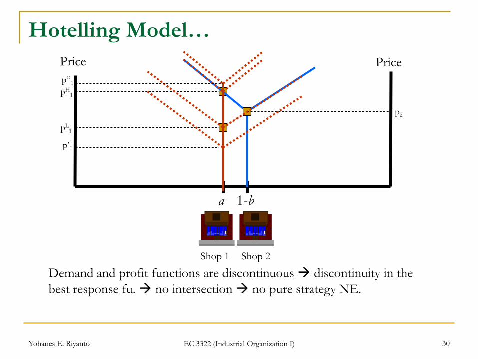
Hotelling Model…
Shop 1 Shop 2
Price Price
1-b a
Demand and profit functions are discontinuous discontinuity in the best response fu. no intersection no pure strategy NE.
p2
pH1
pL1
p’1
p’’1
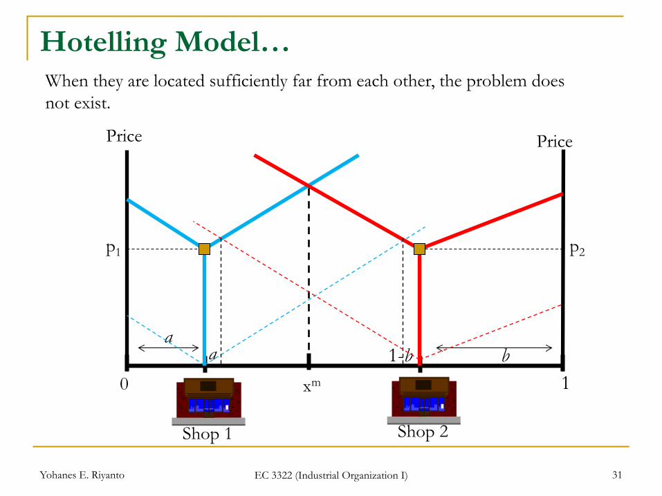
Yohanes E. Riyanto EC 3322 (Industrial Organization I) 31
0 1 xm
a b
Shop 2
1-b
Shop 1
a
Price Price
p1 p2
Hotelling Model… When they are located sufficiently far from each other, the problem does not exist.
Yohanes E. Riyanto EC 3322 (Industrial Organization I) 32
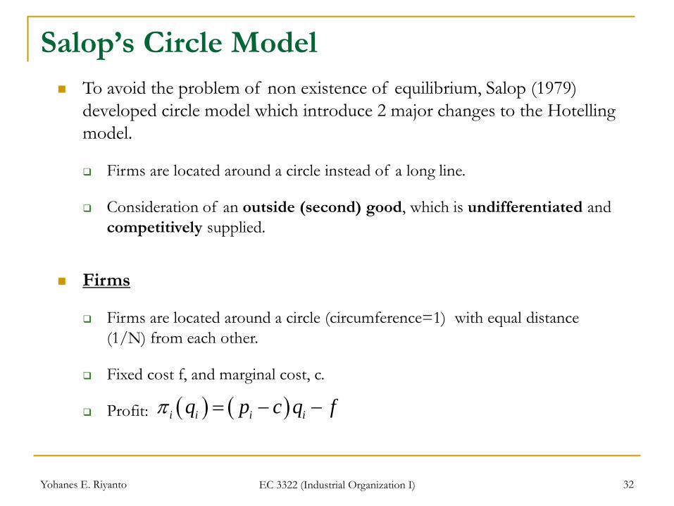
Salop’s Circle Model To avoid the problem of non existence of equilibrium, Salop (1979)
developed circle model which introduce 2 major changes to the Hotelling model.
Firms are located around a circle instead of a long line.
Consideration of an outside (second) good, which is undifferentiated and competitively supplied.
Firms
Firms are located around a circle (circumference=1) with equal distance (1/N) from each other.
Fixed cost f, and marginal cost, c.
Profit:
( ) ( )π = − −i i i iq p c q f
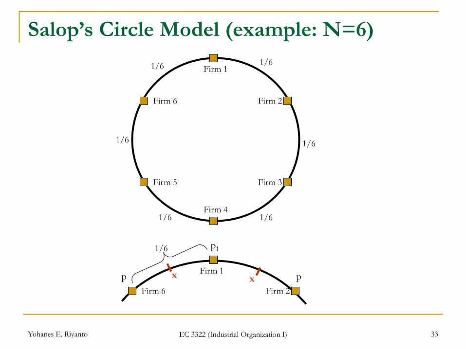
Yohanes E. Riyanto EC 3322 (Industrial Organization I) 33
x
Salop’s Circle Model (example: N=6)
Firm 1
Firm 2
Firm 3
Firm 4
Firm 5
Firm 6
1/6 1/6
1/6
1/6 1/6
1/6
Firm 1
Firm 2 Firm 6
p1
p p x
1/6

Yohanes E. Riyanto EC 3322 (Industrial Organization I) 34
Salop’s Circle Model… Consumers
Uniformly located around the circle (e.g. round the clock airline, bus, and train services, etc).
A consumer’s location x* represents the consumer’s most preferred type of product.
Each consumer buys one unit
Transportation cost per unit of distance = t.
Given the price, p, charged by the adjacent firms (left and right) and p1 charged by firm 1, we can derive the location of the indifferent consumer located at the distance . ( )0,1/∈x N
11 − − = − − −
V p tx V p t x
N
( )1 11
1, 2 −= = +
p pD p p xt N
Firm 1’s market share (demand)

Yohanes E. Riyanto EC 3322 (Industrial Organization I) 35
Salop’s Circle Model… Therefore:
( ) 11 1
11
1
1
0 2 2
π
π
− = − + −
∂= →
∂+
= +
p pp c ft N
pt p cpN
( ) - = + → =t tp c p cN N
By symmetry, we have p1=p, and thus,
Similar as in the Hotelling model, price & profit margin increases with transportation cost t and decrease with N. Suppose that entry by new firms is possible (free-entry) entry will take place until profit is fully dissipated.
( ) 2
1 0π = − − = − =itp c f f
N N and c ctN p c tf
f= = +
Firm’s price is above MC, but yet it earns no profit.

Yohanes E. Riyanto EC 3322 (Industrial Organization I) 36
Salop’s Circle Model… Under free-entry, an increase in fixed cost (f) cause a decrease in the
number of firm (N) and an increase in the profit margin (p-c).
Under free-entry, an increase in transportation cost (t) increases both profit margin (p-c) and the number of firms (N).
When fixed cost (f) falls to zero (0), the number of firms tends to be very large (N infinity).
So far, we have been discussing the case in which firms are located sufficiently close to each other and compete for the same consumers a firm must take into account the price of rivals competitive region (Salop 1979).
If there are only few firms such that they don’t compete for the same consumers each firm is a local monopoly.
0lim
→= = ∞c
f
tNf

Yohanes E. Riyanto EC 3322 (Industrial Organization I) 37
Salop’s Circle Model…
Firm 1
Firm 2
p1
p
1/N
xm1 xm
1
xm2 xm
2
these consumers do not buy since price is higher than the value
obtained (p>V)
1 0− − =V p tx 1−=
V pxc
Indifferent consumer between buying and not buying:
( ) ( )11 1
22= = −D p x V pc
monopoly demand
market is uncovered.
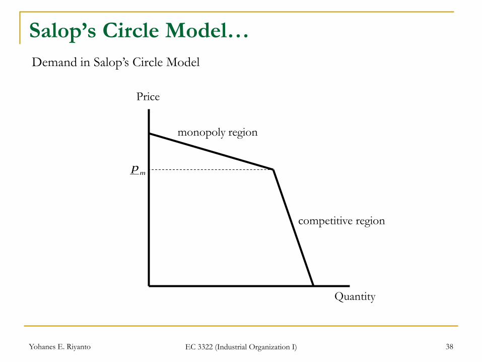
Yohanes E. Riyanto EC 3322 (Industrial Organization I) 38
Salop’s Circle Model…
Price
Quantity
mp
monopoly region
competitive region
Demand in Salop’s Circle Model
Yohanes E. Riyanto EC 3322 (Industrial Organization I) 39
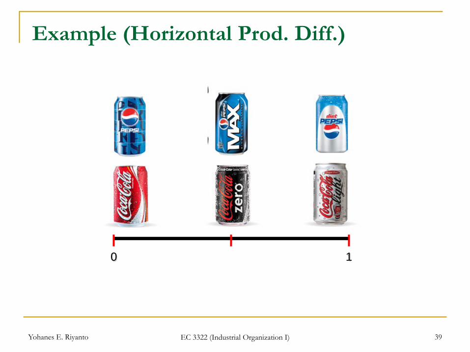
Example (Horizontal Prod. Diff.)
0 1
Yohanes E. Riyanto EC 3322 (Industrial Organization I) 40
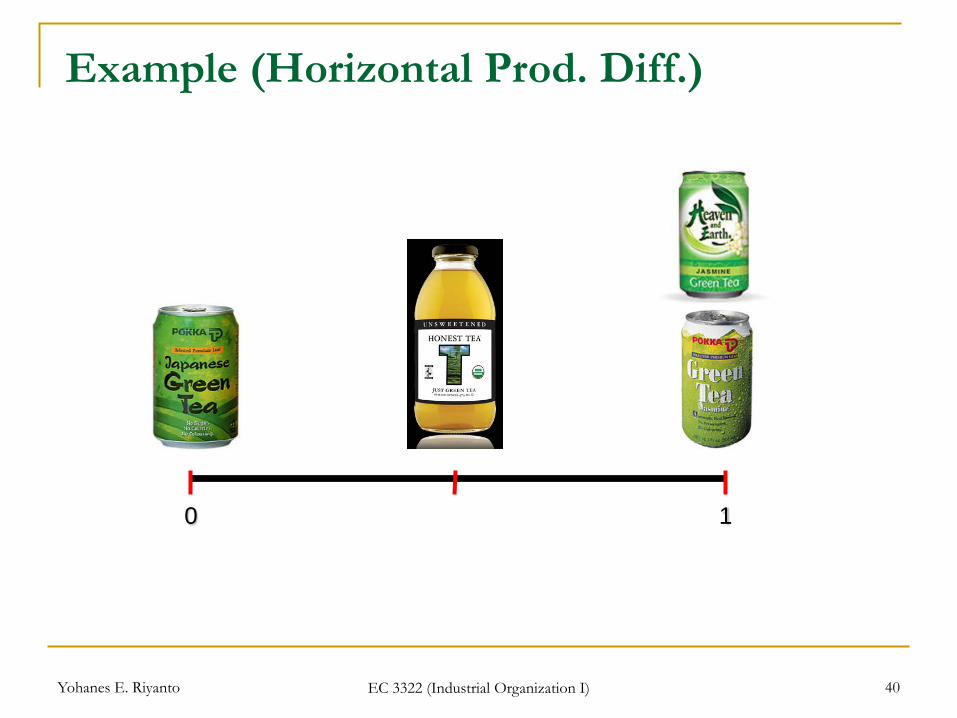
Example (Horizontal Prod. Diff.)
0 1

Yohanes E. Riyanto EC 3322 (Industrial Organization I) 41
DW 2 Tutorial Group
Types of Subscription Plan Number of Students %
Economist.com Subscription US$ 59 14 77.8%
Print & Web Subscription US $125 4 22.2%
TOTAL 18 100%
From Our Mini Class Experiment:
DW I Tutorial Group
Types of Subscription Plan Number of Students %
Economist.com Subscription US$59 10 43.5%
Print Subscription US$125 1 4.3%
Print & Web Subscription US$125 12 52.2%
TOTAL 23 100% Suppose you are a salesman and puts the following display: 36-inch Panasonic $690 42-inch Toshiba $850 50-inch Phillips $1480
Yohanes E. Riyanto EC 3322 (Industrial Organization I) 42
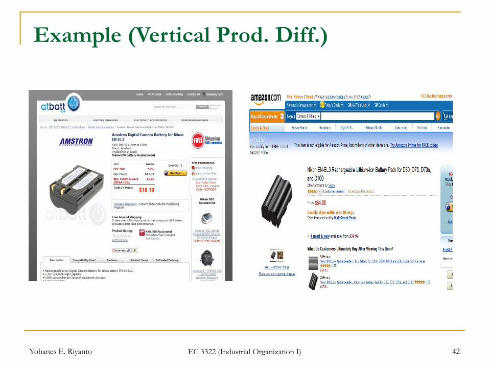
Example (Vertical Prod. Diff.)
Yohanes E. Riyanto EC 3322 (Industrial Organization I) 43
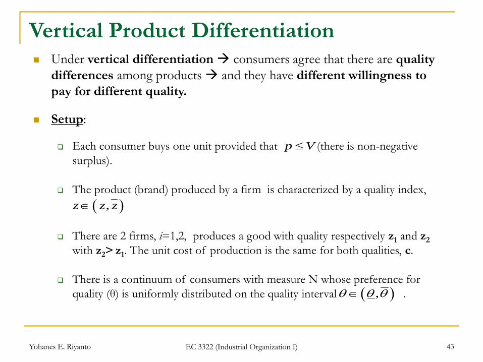
Vertical Product Differentiation Under vertical differentiation consumers agree that there are quality
differences among products and they have different willingness to pay for different quality.
Setup:
Each consumer buys one unit provided that (there is non-negative surplus).
The product (brand) produced by a firm is characterized by a quality index,
There are 2 firms, i=1,2, produces a good with quality respectively z1 and z2 with z2> z1. The unit cost of production is the same for both qualities, c.
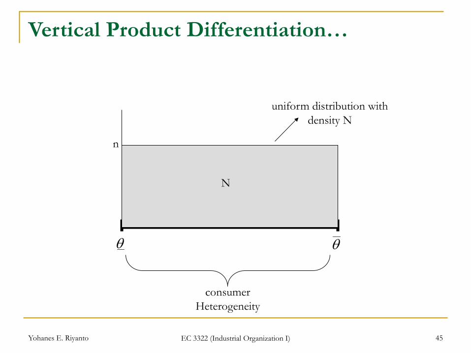
There is a continuum of consumers with measure N whose preference for quality (θ) is uniformly distributed on the quality interval .
( ),z z z∈
( ),θ θ θ∈
≤p V

Yohanes E. Riyanto EC 3322 (Industrial Organization I) 44
lowest quality
highest quality
Vertical Product Differentiation…
consumer taste/ preference &
the range of quality
z
z θ highest value (willingness to pay)
θ lowest value (willingness to pay)
depends on income, taste, etc.
consumer heterogeneity
2z
1z
Senior Consultant
Consultant
Yohanes E. Riyanto EC 3322 (Industrial Organization I) 45
Vertical Product Differentiation…
θθ
n
N
consumer Heterogeneity
uniform distribution with density N
Yohanes E. Riyanto EC 3322 (Industrial Organization I) 46
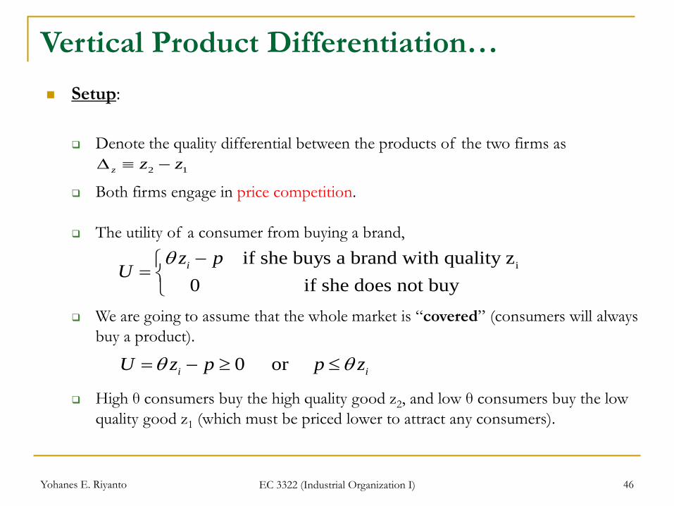
Vertical Product Differentiation… Setup:
Denote the quality differential between the products of the two firms as
Both firms engage in price competition.
The utility of a consumer from buying a brand,
We are going to assume that the whole market is “covered” (consumers will always buy a product).
High θ consumers buy the high quality good z2, and low θ consumers buy the low quality good z1 (which must be priced lower to attract any consumers).
2 1z z z∆ ≡ −
iif she buys a brand with quality z0 if she does not buy
iz pU
θ −=
0 or i iU z p p zθ θ= − ≥ ≤
Yohanes E. Riyanto EC 3322 (Industrial Organization I) 47
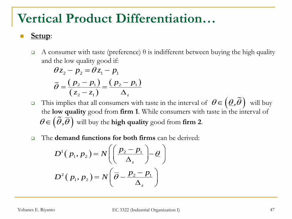
Vertical Product Differentiation… Setup:
A consumer with taste (preference) θ is indifferent between buying the high quality and the low quality good if:
This implies that all consumers with taste in the interval of will buy the low quality good from firm 1. While consumers with taste in the interval of
will buy the high quality good from firm 2.
The demand functions for both firms can be derived:
2 2 1 1z p z pθ θ− = −
( )( )
( )2 1 2 1
2 1 z
p p p pz z
θ − −= =
− ∆( ),θ θ θ∈
( ),θ θ θ∈
( )
( )
1 2 11 2
2 2 11 2
,
,
z
z
p pD p p N
p pD p p N
θ
θ
−= − ∆
−= − ∆

Yohanes E. Riyanto EC 3322 (Industrial Organization I) 48
θθ
n
consumer heterogeneity
uniform distribution with density N
Vertical Product Differentiation…
θ
buy low quality
buy high quality
Yohanes E. Riyanto EC 3322 (Industrial Organization I) 49
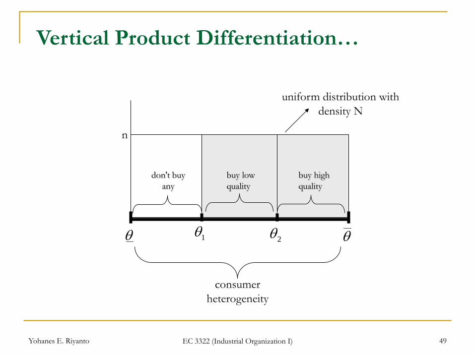
θθ
n
consumer heterogeneity
uniform distribution with density N
Vertical Product Differentiation…
1θ
buy low quality
buy high quality
2θ
don't buy any
Yohanes E. Riyanto EC 3322 (Industrial Organization I) 50
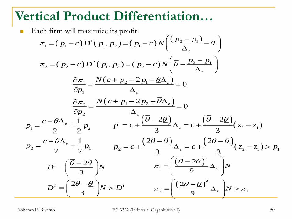
Vertical Product Differentiation… Each firm will maximize its profit.
( ) ( ) ( ) ( )
( ) ( ) ( )
1 2 11 1 1 2 1
2 2 12 2 1 2 2
,
,
z
z
p pp c D p p p c N
p pp c D p p p c N
π θ
π θ
− = − = − − ∆
−= − = − − ∆
( )
( )
2 11
1
1 22
2
20
20
z
z
z
z
N c p pp
N c p pp
θπ
θπ
+ − − ∆∂= =
∂ ∆
+ − + ∆∂= =
∂ ∆
1 2
2 1
12 2
12 2
θ
θ
− ∆= +
+ ∆= +
z
z
cp p
cp p
( ) ( ) ( )
( ) ( ) ( )
1 2 1
2 2 1 1
2 23 3
2 23 3
θ θ θ θ
θ θ θ θ
− −= + ∆ = + −
− −= + ∆ = + − >
z
z
p c c z z
p c c z z p
1
2 1
23
23
D N
D N D
θ θ
θ θ
− =
− = >
( )
( )
2
1
2
2 1
29
29
z
z
N
N
θ θπ
θ θπ π
− = ∆ − = ∆ >
Yohanes E. Riyanto EC 3322 (Industrial Organization I) 51
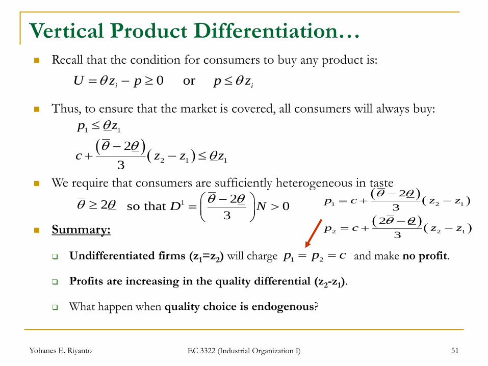
Vertical Product Differentiation… Recall that the condition for consumers to buy any product is:
Thus, to ensure that the market is covered, all consumers will always buy:
We require that consumers are sufficiently heterogeneous in taste
Summary:
Undifferentiated firms (z1=z2) will charge and make no profit.
Profits are increasing in the quality differential (z2-z1).
What happen when quality choice is endogenous?
0 or i iU z p p zθ θ= − ≥ ≤
( ) ( )
1 1
2 1 1
23
p z
c z z z
θ
θ θθ
≤
−+ − ≤
1 2p p c= =
2θ θ≥ 1 2so that 03
θ θ− = >
D N( ) ( )
( ) ( )
1 2 1
2 2 1
23
23
θ θ
θ θ
−= + −
−= + −
p c z z
p c z z
Yohanes E. Riyanto EC 3322 (Industrial Organization I) 52
Vertical Product Differentiation… Endogenous choice of quality.
Suppose now, firms play a two-stage game, in which firms first choose quality (one per firm) and then compete in price.
Assume for simplicity that the choice of quality is costless. Firms choose zi from the interval
Since the size of profit depends on (z2-z1), for a given z2 firm 1 wants to choose z1 as lowest as possible (z1= ). For a given z1, firm 2 wants to set z2 is high as possible (z2= ).
A similar result is obtained if instead firm 1 is the one which produces high quality.
There are two pure strategy Nash equilibria, the first one is (z1= , z2= ), the second one is (z1= , z2= ).
In equilibrium, we have maximal differentiation relaxing price competition through product differentiation.
( ),iz z z∈
zz
z zz z
Yohanes E. Riyanto EC 3322 (Industrial Organization I) 53
Vertical Product Differentiation… Endogenous choice of quality.
In a Stackelberg setting, the first mover always wants to enter with high quality, and given this the second mover will choose low quality this gives us a unique equilibrium.
We have a setting in which choice of quality is costless and yet, the low quality firm gains from reducing its quality level to the minimum trade-off: demand reduction because of lower quality vs. softer price competition.