Embed Size (px)
Citation preview
Title Analysis and flamelet modelling for spray combustion
Author(s) Baba, Yuya; Kurose, Ryoichi
Citation Journal of Fluid Mechanics (2008), 612: 45-79
Issue Date 2008-10-10
URL http://hdl.handle.net/2433/88947
Right Copyright © Cambridge University Press 2008
Type Journal Article
Textversion publisher
Kyoto University
J. Fluid Mech. (2008), vol. 612, pp. 45–79. c© 2008 Cambridge University Press
doi:10.1017/S0022112008002620 Printed in the United Kingdom
45
Analysis and flamelet modellingfor spray combustion
YUYA BABA1 AND RYOICHI KUROSE2
1Earth Simulator Center, Japan Agency for Marine-Earth Science and Technology (JAMSTEC),3173-25 Showa-machi, Kanazawa-ku Yokohama, Kanagawa 236-0001, Japan
[email protected] of Mechanical Engineering and Science, and Advanced Research Institute of FluidScience and Engineering, Kyoto University, Yoshida-honmachi, Sakyo-ku, Kyoto 606-8501, Japan
(Received 21 February 2007 and in revised form 19 May 2008)
The validity of a steady-flamelet model and a flamelet/progress-variable approach forgaseous and spray combustion is investigated by a two-dimensional direct numericalsimulation (DNS) of gaseous and spray jet flames, and the combustion characteristicsare analysed. A modified flamelet/progress-variable approach, in which total enthalpyrather than product mass fraction is chosen as a progress variable, is also examined.DNS with an Arrhenius formation, in which the chemical reaction is directly solvedin the physical flow field, is performed as a reference to validate the combustionmodels. The results show that the diffusion flame is dominant in the gaseous diffusionjet flame, whereas diffusion and premixed flames coexist in the spray jet flame.The characteristics of the spray flame change from premixed–diffusion coexistentto diffusion-dominant downstream. Comparisons among the results from DNS withvarious combustion models show the modified flamelet/progress-variable approach tobe superior to the other combustion models, particularly for the spray flame. Wherethe behaviour of the gaseous total enthalpy is strongly affected by the energy transfer(i.e. heat transfer and mass transfer) from the dispersed droplet, and this effect canbe accounted for only by solving the conservation equation of the total enthalpy.However, even the DNS with the modified flamelet/progress-variable approach tendsto underestimate the gaseous temperature in the central region of the spray jet flame.To increase the prediction accuracy, a combustion model for the partially premixedflame for the spray flame is necessary.
1. IntroductionSpray combustion is utilized in a number of engineering applications, such as energy
conversion and propulsion devices. It is therefore necessary to precisely predict thecombustion behaviour of the fuel spray when designing and operating equipment.However, since spray combustion is a complex phenomenon, in which the dispersionof fuel droplets, their evaporation and a chemical reaction of the fuel vapour withoxidizer take place simultaneously and interact with each other, the underlying physicsgoverning these processes have not been well established. In order to understandthe spray combustion behaviour, numerical simulations based on direct numericalsimulations (DNS) or large-eddy simulations (LES) have recently been performed.
DNS is an appropriate tool for discussing the detailed spray combustion mechanismassociated with the interaction between turbulence and reaction, since all scales for
46 Y. Baba and R. Kurose
chemical reactions as well as hydrodynamics are resolved simultaneously. Reveillon& Vervisch (2005) and Domingo, Vervisch & Reveillon (2005) performed two-dimensional DNS of spray jet flames and discussed the detailed characteristics in termsof the topology of the droplet group combustion regimes and the partially premixedmodel, respectively. Nakamura et al. (2005) also investigated the droplet groupcombustion behaviour, under various droplet-size and equivalence-ratio conditionsby two-dimensional DNS of spray flames formed in laminar counterflow diffusionflames. Watanabe et al. (2007, 2008) extended the work of Nakamura et al. (2005)and discussed the flamelet characteristics of the spray flames. These works revealthat at present the DNS of spray flames is limited to two-dimensional simulations,since limits on computational costs make it impossible to conduct three-dimensionalsimulations to clarify the three-dimensional spray flame behaviour.
On the other hand, LES, in which the gaseous-phase behaviour is spatiallyfiltered and the unresolved scales are modelled by subgrid-scale (SGS) models, isattractive, since it can be applied to three-dimensional spray combustion fields evenfor large-scale industrial devices. Ham et al. (2003) and Kurose et al. (2003, 2004)performed LES of an turbulent spray combustion in a realistic gas turbine and asolid/spray jet flame, respectively, and discussed the validity. These works appear tobe successful, but also reveal a further question concerning the combustion modelfor spray flames, as follows.
In LES or RANS (Reynolds-averaged Navier–Stokes) modelling of gaseous fueldiffusion combustion, the flamelet models proposed by Peters (1984, 2000) have beenwidely used in different formulations such as the steady-flamelet model (Cook, Riley& Kosaly 1997), unsteady-flamelet model (Pitsch 2000; Pitsch & Steiner 2000), andflamelet/progress-variable approach (Pierce & Moin 2004). In these flamelet models,in general, the conservation equations of mass, momentum and mixture fraction Z
as a conserved scalar are solved in the flow field (physical space), and temperatureand chemical species mass fractions at each position are identified by referring to adatabase, a so-called ‘chemtable’ (i.e. chemistry table, flamelet library). The chemtableis obtained by solving a one-dimensional flamelet equation in the Z space, and Z
and the scalar dissipation rate χ (=2DZ∇Z·∇Z) are used as parameters to relate thephysical space to the Z space. Here, DZ is the diffusion coefficient of Z.
For the spray combustion, on the other hand, Z is no longer a conserved scalarbecause of the mass transfer (i.e. evaporation of fuel) between the dispersed dropletphase and the carrier gaseous phase (Watanabe et al. 2007, 2008). Consequently,the behaviour of variables such as temperature and chemical species mass fractionsversus Z and χ in two-phase combustion becomes complicated and cannot beidentified by these parameters alone. In addition, without solving the energy equation,the heat transfer between the dispersed droplet phase and the carrier gaseous phasecannot be taken into account. The heat transfer, including the heat loss due to dropletevaporation, which is referred to as the droplet cooling effect, is found to affect thespray flame temperature (Nakamura et al. 2005). Although Hollmann & Gutheil(1998) proposed a steady-flamelet-based model for spray flames, their modellingneeds many parameters to account for the spray characteristics and lacks universality.The flamelet/progress-variable approach proposed by Pierce & Moin (2004), whichemploys an additional parameter called the progress variable to capture the flame lift,local extinction and re-ignition dynamics, may also improve the numerical accuracyfor spray combustion, because this approach can provide intrinsic informationconcerning the relation between Z and the chemical reaction. In the original model,however, again the heat transfer between the phases cannot be considered, since
Analysis and flamelet modelling for spray combustion 47
a product mass fraction unrelated to thermal energy is chosen as the progressvariable.
In this study, we propose a modified flamelet/progress-variable approach, in whichenthalpy is employed as the progress variable (referred to as FPVA-E, hereafter),and its applicability to gaseous and spray flames is investigated by performing two-dimensional DNS of gaseous and spray jet flames. The results are compared withcases where an Arrhenius formation, a steady-flamelet model and the conventionalflamelet/progress-variable approach, in which the product mass fraction is chosen asthe progress variable, are employed as the combustion models (referred to as ARF,SFM and FPVA-P, respectively), and the detailed spray combustion mechanism isdiscussed in terms of the modelling. Originally, combustion models such as SFM andFPVA were intended for use in connection with SGS models for LES or RANS ofthe carrier gaseous phase. However, in order to avoid discussion of the effect of theSGS contributions on numerical accuracy, a numerical method using fine resolutionwithout the SGS models is chosen here. In this paper, we simply call this methodDNS, regardless of the combustion model.
The numerical procedure, including the governing equations, combustion models,and numerical conditions, is described in §2. The detailed combustion behaviour andthe validity of the combustion models are discussed for gaseous combustion and spraycombustion in §3 and §4, respectively. Finally, the main findings are summarized in §5.
2. Numerical simulationsIn this paper, we refer to the numerical method, in which non-filtered and non-
averaged equations of the carrier gaseous phase are solved, as DNS regardlessof the combustion model. The combustion models compared are the Arrheniusformation (ARF), steady-flamelet model (SFM), and flamelet/progress-variableapproach (FPVA). It is assumed that DNS with ARF reveals true flame behaviour.
2.1. Governing equations for DNS with Arrhenius formation (ARF)
The conservation equations of the mass, momentum, internal energy and massfractions of chemical species are solved to describe the carrier gaseous phasebehaviour. The set of governing equations based on a low-Mach-number formulationis (Nakamura et al. 2005)
∂ρ
∂t+
∂ρuj
∂xj
= Sρ, (2.1)
∂ρui
∂t+
∂ρujui
∂xj
= − ∂p
∂xi
+∂σij
∂xj
+ Sui, (2.2)
∂ρh
∂t+
∂ρujh
∂xj
=∂
∂xj
(ρa
∂h
∂xj
)+ Sh, (2.3)
∂ρYi
∂t+
∂ρujYi
∂xj
=∂
∂xj
(ρDi
∂Yi
∂xj
)+ mi + SYi
, (2.4)
where ρ, ui , h, Yi are the density, velocity, total enthalpy and mass fraction of theith species, respectively; mi is the mass production or consumption rate of the ithspecies, as shown later; σij is the viscous stress tensor given by
σij = μ
(∂ui
∂xj
+∂uj
∂xi
)− 2
3μδij
∂uk
∂xk
, (2.5)
48 Y. Baba and R. Kurose
where μ is the viscosity. In (2.3), the diffusion coefficient of the enthalpy a is givenby ρa = λ/cp . In (2.4), the unity Lewis number assumption, in which all diffusioncoefficients of species are given by ρDi = λ/cp , is introduced.
The phase coupling is implemented using a Eulerian/Lagrangian method. Sρ , Sui,
Sh and SYiare the phase coupling terms between the carrier gaseous phase and the
dispersed droplet phase given as
Sρ = − 1
�V
∑N
dmd
dt, (2.6)
Sui= − 1
�V
∑N
d
dt(mdvi) , (2.7)
Sh = − 1
�V
∑N
[1
2
d
dt(mdvivi) +
d
dt(cLmdTd)
], (2.8)
SYi= − 1
�V
∑N
dmd
dtfor Yi = YV , (2.9)
where cL is the heat capacity of the droplet, �V the control volume and YV themass fraction of fuel vapour. Summation
∑N denotes the contributions of sources
surrounding the liquid droplets, from the dispersed phase to the carrier gaseous phase.Linear interpolation and extrapolation with weighting factors are used for the phasecoupling (Miller & Bellan 1999). Other variables will be explained later.
Individual droplets are tracked in a Lagrangian framework under the assumptionthat the droplet volume is negligible. The governing equations for the droplet positionXi , velocity vi , temperature Td and mass md are given by (Miller, Harstad & Bellan1998)
dXi
dt= vi, (2.10)
dvi
dt=
Fi
md
=
(f1
τd
)(ui − vi) , (2.11)
dTd
dt=
Qd + mdLV
mdcL
=Nu
3Pr
(f2
τd
)(cp
cL
)(T − Td) +
md
md
LV
cL
, (2.12)
dmd
dt= md = −md
τd
(Sh
3Sc
)ln (1 + BM ) , (2.13)
where Fi is the drag force, Qd is the heat flux, LV is the latent heat of dropletevaporation, given as a function of the droplet temperature and Nu, Pr, Sh and Scare the Nusselt, Prandtl, Sherwood and Schmidt number, defined below.
The particle response time of the droplet is τd defined by
τd =ρdd
2d
18μ, (2.14)
where ρd and dd are the droplet density and diameter, respectively. The internaldroplet temperature and density are assumed to be uniform. In addition, the lift forcedue to fluid shear and breakup and collision of the droplets are neglected (Kurose& Komori 1999; Apte, Gorokhovski & Moin 2003). As will be shown later, dropletsbecome dense close to the injector and, in this area, spray dispersion is not realistic.
Analysis and flamelet modelling for spray combustion 49
However, because the combustion phenomena far from the injector are focused on inthis study, these assumptions are considered to be acceptable.
The mass transfer number BM is calculated from the mass fraction of the fuel inthe carrier gaseous phase YV and that at the droplet’s surface YV,s as
BM = (YV,s − YV )/(1 − YV )
YV,s is evaluated using the Clausius–Clapeyron relation under the saturation pressurecondition as
YV,s =XV,s
XV,s +(1 − XV,s
)W/WV
, (2.15)
XV,s =Patm
Pexp
[LV
RV
(1
TBL
− 1
Td
)]−
(2Lk
dd
)β, (2.16)
where XV,s is the mole fraction of fuel vapour at the droplet surface, Patm is theatmospheric pressure, P is the pressure of the carrier gaseous phase, RV is the gasconstant for fuel vapour, and TBL is the boiling temperature of the liquid droplet.W and WV are the averaged molecular weights of the carrier gaseous phase and themolecular weight of the fuel vapour, respectively. In (2.16), a non-equilibrium effectis considered using the Langmuir–Knudsen evaporation law (Bellan & Summerfield1978); β is the non-dimensional evaporation parameter given by
β = −(
ρdP r
8μ
)dd2
d
dt. (2.17)
The value of the Knudsen layer thickness Lk is computed by
Lk =μ [2πTd(R/WV )]1/2
ScP, (2.18)
where R is the universal gas constant. The Nusselt and Sherwood numbers are givenbased on the Ranz–Marshall correlation as
Nu = 2 + 0.552Re1/2sl P r1/3, Sh = 2 + 0.552Re
1/2sl Sc1/3. (2.19)
The modified correlation for the drag force, the reduction effect due to includingblowing velocity, is (Kurose et al. 2003)
f1 =1 + 0.0545Resl + 0.1Re
1/2sl (1 − 0.03Resl)
1 + b|Reb|c , (2.20)
b = 0.06 + 0.077 exp(−0.4Resl), c = 0.4 + 0.77 exp(−0.04Resl), (2.21)
where Resl = ρusldd/μ and Reb = ρubdd/μ are the particle Reynolds numbers basedon the slip velocity usl = |ui − vi | and the blowing velocity ub, respectively. On theother hand, f2 is the correction to the heat transfer given by f2 = β/(eβ − 1).
A one-step global reaction of n-decane oxidation,
C10H22 + 31/2O2 → 10CO2 + 11H2O, (2.22)
is considered here to reduce the computational cost. In ARF, the mass consumptionrate of the evaporated fuel (n-decane) mV is given by (Westbrook & Dryer 1984)
mV = WV AT n
(ρYV
WV
)a (ρYO
WO
)b
exp
(− E
RT
). (2.23)
50 Y. Baba and R. Kurose
Here, A is the pre-exponential factor, E the activation energy, and n, a and b thecoefficients for hydrocarbon fuels. WO is the molecular weight of the oxidizer andYV , YO are the mass fractions of the fuel and oxidizer, respectively. For the n-decaneoxidation reaction, those constants are A = 3.8 × 10¹¹, E = 30 kcal, n = 0, a = 0.25and b = 1.5. The chemical species considered are C10H22, CO2, H2O, O2 and N2, andtheir production or consumption rates mi in (2.4) are calculated by using the value ofmV and the equivalence relation. The thermodynamics and transport properties suchas viscosity and thermal conductivity are calculated using the CHEMKIN database(Kee et al. 1986; Kee, Rupley & Miller 1989).
2.2. Steady-flamelet model (SFM)
In SFM, the conservation equations of mass (2.1), momentum (2.2), and the transportequation of the mixture fraction Z are solved for the carrier gaseous phase in thephysical space, and temperature and chemical species mass fractions at each positionare obtained by referring to a chemtable. In general, the chemtable is generatedbeforehand by solving a one-dimensional flamelet equation in the Z space andtabulating variables such as the temperature and chemical species mass fractions,with respect to Z and the scalar dissipation rate
χ = 2DZ
∂Z
∂xj
∂Z
∂xj
, (2.24)
where DZ is the diffusion coefficient of Z, which is given by ρDZ = λ/cp under theunity Lewis number assumption. It is considered that χ characterizes the strain rateof the local flame structure.
The transport equation of Z is
∂ρZ
∂t+
∂ρujZ
∂xj
=∂
∂xj
(ρDZ
∂Z
∂xj
)+ SZ. (2.25)
Here, the phase coupling term with evaporating droplets, SZ , is required only for thespray combustion, not for the gaseous combustion. This is derived as follows. Thedefinition of Z is
Z =φYV /YV,0 − YO/YO,0 + 1
φ + 1, (2.26)
where YV,0 and YO,0 are the mass fractions of fuel vapour and oxidizer in Z space (i.e.YV,0 = 1.0 and YO,0 = 0.2324), respectively; φ is the chemical equivalence ratio definedas φ = (νOWOYV,0)/(νV WV YO,0), where νO and νV are the stoichiometric coefficientsof oxidizer and fuel of the n-decane oxidation reaction, respectively. The source termof Z in (2.25), SZ is derived in conservative form using relation (2.26) as
∂ρZ
∂t=
1
φ + 1
(φ
YV,0
∂ρYV
∂t− 1
YO,0
∂ρYO
∂t+
∂ρ
∂t
). (2.27)
Here, the time variations of YV and YO due to the droplet evaporation are
∂ρYV
∂t= SYV
,∂ρYO
∂t= 0. (2.28)
This leads to SZ being
SZ =∂ρZ
∂t=
1
φ + 1
(φSYV
− 0 + SYV
)= SYV
. (2.29)
Analysis and flamelet modelling for spray combustion 51
Here, the relation of the time variation of ρ due to the droplet evaporation, ∂ρ/∂t =Sρ = SYV
, is used.In SFM, variables such as the gaseous temperature and chemical species mass
fractions are obtained from the chemtable using the two parameters Z and χ , asdescribed earlier. Hence, these variables can be expressed as functions of Z and χ , i.e.
T = T (Z, χ), Yi = Yi(Z, χ). (2.30)
2.3. Flamelet/progress-variable approach (FPVA)
In FPVA, the conservation equations of mass (2.1), momentum (2.2), and the transportequations of Z (2.25) and one additional tracking scalar called the progress variableC are solved. The progress variable C must be non-conserved, independent of Z, andcharacterize χ as
χ = χ(Z, C). (2.31)
Consequently, the variables in reacting flows are represented by the referenceparameters of Z and C, rather than Z and χ in SFM. This can be expressedas
T = T (Z, C), Yi = Yi(Z, C). (2.32)
It should be noted here that the chemtables used for SFM and FPVA are essentiallyidentical.
In the conventional FPVA proposed by Pierce & Moin (2004), the product massproduction is chosen as C (=YCO2 + YH2O) (referred to as FPVA-P). The transportequation is
∂ρC
∂t+
∂ρujC
∂xj
=∂
∂xj
(ρDC
∂C
∂xj
)+ ρωC, (2.33)
where DC is the diffusion coefficient of C, which is given by ρDC = λ/cp under theunity Lewis number assumption; ωC is the production rate of C. The definition of C
leads ωC to be a sum of the mass production rates of combustion products as
ρωC = mCO2 + mH2O. (2.34)
This value is obtained from the chemtable. Pierce & Moin state that this FPVA-Pis superior to SFM in capturing and reproducing flame lift, local extinction and re-ignition dynamics, because it provides intrinsic information about chemical reaction.However, the heat transfer between the dispersed droplet phase and carrier gaseousphase cannot be taken into account. Therefore, we propose a modified FPVA usingtotal enthalpy h =
∑N
i=1 hiYi as C (referred to as FPVA-E).In gaseous combustion, the total enthalpy generally cannot be the progress variable.
This is because the behaviour of the total enthalpy is very similar to that of the mixturefraction. As discussed later, however, the total enthalpy can be the progress variablewhen there exists a specific boundary condition for the total enthalpy or the totalenthalpy is not a conserved scalar such that the last term (source term) on the right-hand side of (2.3) is non-zero. These conditions appear when high-temperature coflowfor the flame stabilization, heat loss from walls (Pitsch & Duchamp de Lageneste2002), radiation and so on are considered. In spray combustion, on the other hand,the total enthalpy can be the progress variable in spite of the above conditions, sinceit varies as the reaction proceeds through fuel evaporation. This is evident from (2.3),in which the last term (source term) on the right-hand side could be non-zero, aswritten below again.
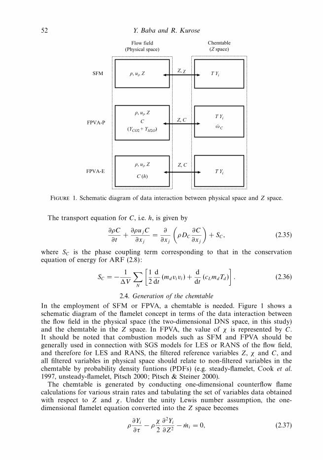
52 Y. Baba and R. Kurose
Flow field(Physical space)
Chemtable(Z space)
SFM
FPVA-P
FPVA-E
ρ, ui, Z
ρ, ui, Z
ρ, ui, ZT Yi
T Yi
T Yi
C
(YCO2 + YH2O)
C (h)
Z, χ
Z, C
Z, C
ω C
Figure 1. Schematic diagram of data interaction between physical space and Z space.
The transport equation for C, i.e. h, is given by
∂ρC
∂t+
∂ρujC
∂xj
=∂
∂xj
(ρDC
∂C
∂xj
)+ SC, (2.35)
where SC is the phase coupling term corresponding to that in the conservationequation of energy for ARF (2.8):
SC = − 1
�V
∑N
[1
2
d
dt(mdvivi) +
d
dt(cLmdTd)
]. (2.36)
2.4. Generation of the chemtable
In the employment of SFM or FPVA, a chemtable is needed. Figure 1 shows aschematic diagram of the flamelet concept in terms of the data interaction betweenthe flow field in the physical space (the two-dimensional DNS space, in this study)and the chemtable in the Z space. In FPVA, the value of χ is represented by C.It should be noted that combustion models such as SFM and FPVA should begenerally used in connection with SGS models for LES or RANS of the flow field,and therefore for LES and RANS, the filtered reference variables Z, χ and C, andall filtered variables in physical space should relate to non-filtered variables in thechemtable by probability density funtions (PDFs) (e.g. steady-flamelet, Cook et al.1997, unsteady-flamelet, Pitsch 2000; Pitsch & Steiner 2000).
The chemtable is generated by conducting one-dimensional counterflow flamecalculations for various strain rates and tabulating the set of variables data obtainedwith respect to Z and χ . Under the unity Lewis number assumption, the one-dimensional flamelet equation converted into the Z space becomes
ρ∂Yi
∂τ− ρ
χ
2
∂2Yi
∂Z2− mi = 0, (2.37)
Analysis and flamelet modelling for spray combustion 53
101 100 101 102
500
1000
1500
2000
Scalar dissipation rate, χ (s–1)
Tem
pera
ture
, Tm
ax (
K)
(2)(1)
(3)
Unstable branch
Steady burning branchCritical point
Unburned branch
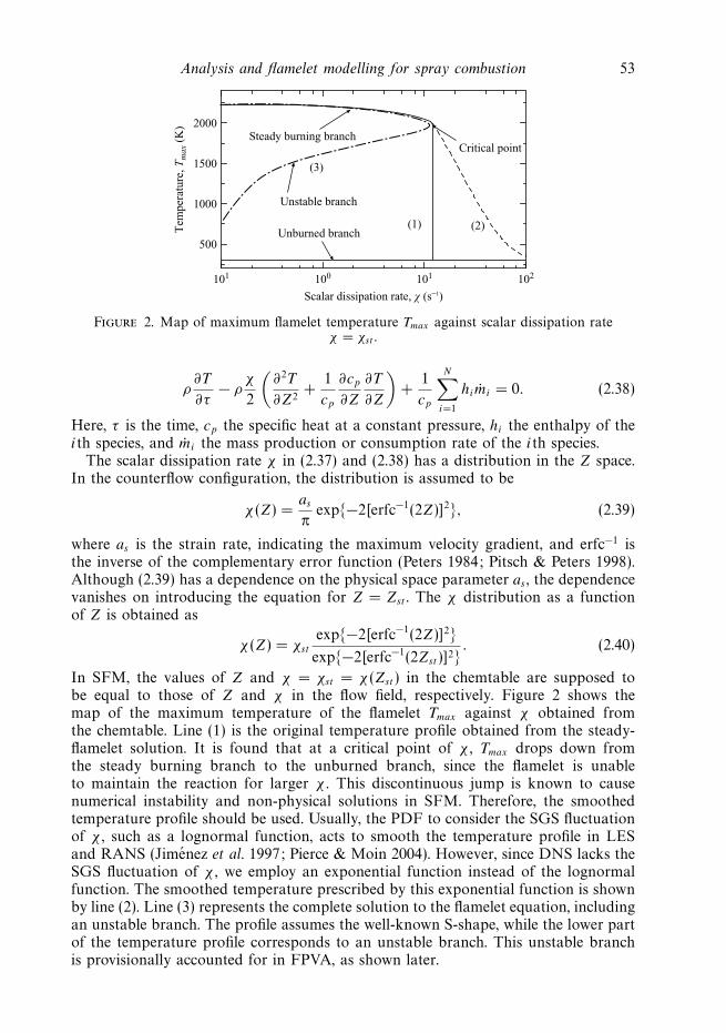
Figure 2. Map of maximum flamelet temperature Tmax against scalar dissipation rateχ = χst .
ρ∂T
∂τ− ρ
χ
2
(∂2T
∂Z2+
1
cp
∂cp
∂Z
∂T
∂Z
)+
1
cp
N∑i=1
himi = 0. (2.38)
Here, τ is the time, cp the specific heat at a constant pressure, hi the enthalpy of theith species, and mi the mass production or consumption rate of the ith species.
The scalar dissipation rate χ in (2.37) and (2.38) has a distribution in the Z space.In the counterflow configuration, the distribution is assumed to be
χ(Z) =as
πexp{−2[erfc−1(2Z)]2}, (2.39)
where as is the strain rate, indicating the maximum velocity gradient, and erfc−1 isthe inverse of the complementary error function (Peters 1984; Pitsch & Peters 1998).Although (2.39) has a dependence on the physical space parameter as , the dependencevanishes on introducing the equation for Z = Zst . The χ distribution as a functionof Z is obtained as
χ(Z) = χst
exp{−2[erfc−1(2Z)]2}exp{−2[erfc−1(2Zst )]2}
. (2.40)
In SFM, the values of Z and χ = χst = χ(Zst ) in the chemtable are supposed tobe equal to those of Z and χ in the flow field, respectively. Figure 2 shows themap of the maximum temperature of the flamelet Tmax against χ obtained fromthe chemtable. Line (1) is the original temperature profile obtained from the steady-flamelet solution. It is found that at a critical point of χ , Tmax drops down fromthe steady burning branch to the unburned branch, since the flamelet is unableto maintain the reaction for larger χ . This discontinuous jump is known to causenumerical instability and non-physical solutions in SFM. Therefore, the smoothedtemperature profile should be used. Usually, the PDF to consider the SGS fluctuationof χ , such as a lognormal function, acts to smooth the temperature profile in LESand RANS (Jimenez et al. 1997; Pierce & Moin 2004). However, since DNS lacks theSGS fluctuation of χ , we employ an exponential function instead of the lognormalfunction. The smoothed temperature prescribed by this exponential function is shownby line (2). Line (3) represents the complete solution to the flamelet equation, includingan unstable branch. The profile assumes the well-known S-shape, while the lower partof the temperature profile corresponds to an unstable branch. This unstable branchis provisionally accounted for in FPVA, as shown later.
54 Y. Baba and R. Kurose
0 0.2 0.4 0.6 0.8 1.0
0.1
0.2
0.3
Z0 0.2 0.4 0.6 0.8 1.0
Z
C
(a)
–1.5
–1.0
–0.5
0
(×106)
χ = 0.5 s–1
χ = 2.5 s–1
χ = 5.0 s–1
χ = 7.5 s–1
χ = 9.0 s–1
χ = 12.0 s–1
(b)
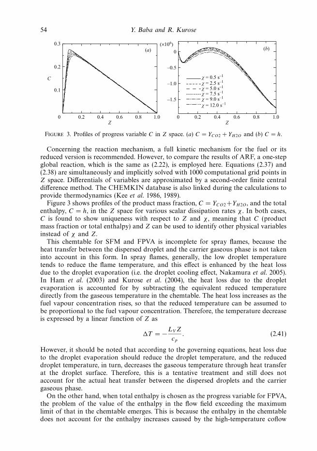
Figure 3. Profiles of progress variable C in Z space. (a) C = YCO2 + YH2O and (b) C = h.
Concerning the reaction mechanism, a full kinetic mechanism for the fuel or itsreduced version is recommended. However, to compare the results of ARF, a one-stepglobal reaction, which is the same as (2.22), is employed here. Equations (2.37) and(2.38) are simultaneously and implicitly solved with 1000 computational grid points inZ space. Differentials of variables are approximated by a second-order finite centraldifference method. The CHEMKIN database is also linked during the calculations toprovide thermodynamics (Kee et al. 1986, 1989).
Figure 3 shows profiles of the product mass fraction, C = YCO2 +YH2O , and the totalenthalpy, C = h, in the Z space for various scalar dissipation rates χ . In both cases,C is found to show uniqueness with respect to Z and χ , meaning that C (productmass fraction or total enthalpy) and Z can be used to identify other physical variablesinstead of χ and Z.
This chemtable for SFM and FPVA is incomplete for spray flames, because theheat transfer between the dispersed droplet and the carrier gaseous phase is not takeninto account in this form. In spray flames, generally, the low droplet temperaturetends to reduce the flame temperature, and this effect is enhanced by the heat lossdue to the droplet evaporation (i.e. the droplet cooling effect, Nakamura et al. 2005).In Ham et al. (2003) and Kurose et al. (2004), the heat loss due to the dropletevaporation is accounted for by subtracting the equivalent reduced temperaturedirectly from the gaseous temperature in the chemtable. The heat loss increases as thefuel vapour concentration rises, so that the reduced temperature can be assumed tobe proportional to the fuel vapour concentration. Therefore, the temperature decreaseis expressed by a linear function of Z as
�T = −LV Z
cp
. (2.41)
However, it should be noted that according to the governing equations, heat loss dueto the droplet evaporation should reduce the droplet temperature, and the reduceddroplet temperature, in turn, decreases the gaseous temperature through heat transferat the droplet surface. Therefore, this is a tentative treatment and still does notaccount for the actual heat transfer between the dispersed droplets and the carriergaseous phase.
On the other hand, when total enthalpy is chosen as the progress variable for FPVA,the problem of the value of the enthalpy in the flow field exceeding the maximumlimit of that in the chemtable emerges. This is because the enthalpy in the chemtabledoes not account for the enthalpy increases caused by the high-temperature coflow
Analysis and flamelet modelling for spray combustion 55
x∗
y∗
OFuel
Air
Air
Coflow
Coflow
Z = 0,U∗ = 1
Z = 0, U∗ = 1
Z = Zst, U∗ = 5
Z = Zst, U∗ = 5
Z = 0 or Z = 1U∗ = 5
y∗1
y∗2
y∗1
y∗2
Figure 4. Schematic of computational domain and inlet conditions.
in flame stabilization nor the mass transfer from droplets to the gaseous phase dueto the evaporation in the flow field. To take this effect into account, the temperatureincrease is calculated by
�T =C − Cc
cp
. (2.42)
This temperature modification is applied only when the enthalpy in the flow field C
exceeds the upper limit of that in the chemtable Cc.The above two temperature modifications, (2.41) and (2.42), are conducted as a
post-process of the chemtable generation, because these effects cannot be includedin the one-dimensional flamelet equation. The gaseous temperature modified in thismanner is used in the computation of the flow field. The validity of these modificationswill be discussed later.
2.5. Numerical conditions
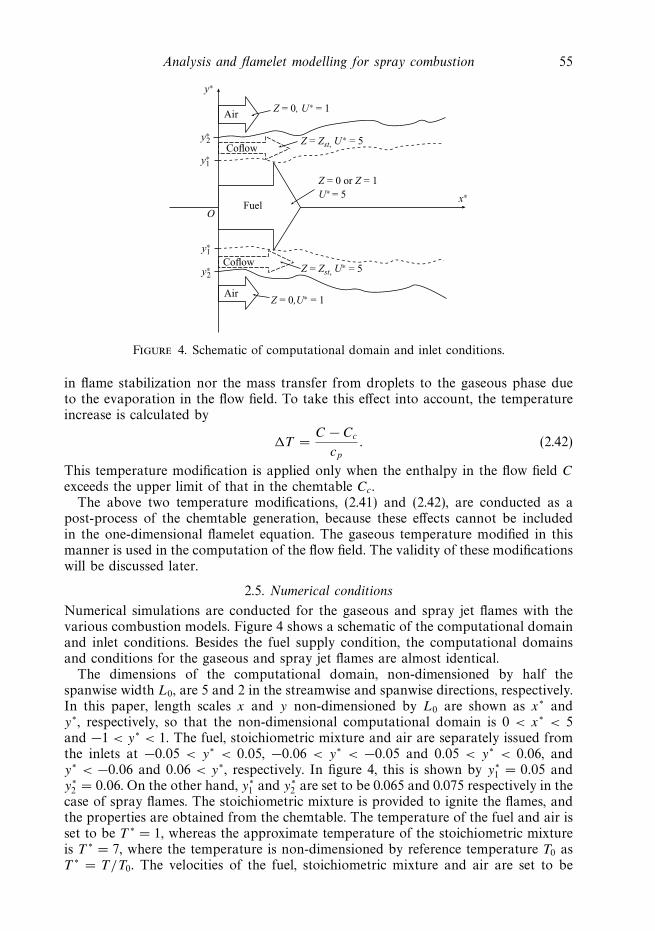
Numerical simulations are conducted for the gaseous and spray jet flames with thevarious combustion models. Figure 4 shows a schematic of the computational domainand inlet conditions. Besides the fuel supply condition, the computational domainsand conditions for the gaseous and spray jet flames are almost identical.
The dimensions of the computational domain, non-dimensioned by half thespanwise width L0, are 5 and 2 in the streamwise and spanwise directions, respectively.In this paper, length scales x and y non-dimensioned by L0 are shown as x∗ andy∗, respectively, so that the non-dimensional computational domain is 0 < x∗ < 5and −1 < y∗ < 1. The fuel, stoichiometric mixture and air are separately issued fromthe inlets at −0.05 < y∗ < 0.05, −0.06 < y∗ < −0.05 and 0.05 < y∗ < 0.06, andy∗ < −0.06 and 0.06 < y∗, respectively. In figure 4, this is shown by y∗
1 = 0.05 andy∗
2 = 0.06. On the other hand, y∗1 and y∗
2 are set to be 0.065 and 0.075 respectively in thecase of spray flames. The stoichiometric mixture is provided to ignite the flames, andthe properties are obtained from the chemtable. The temperature of the fuel and air isset to be T ∗ = 1, whereas the approximate temperature of the stoichiometric mixtureis T ∗ = 7, where the temperature is non-dimensioned by reference temperature T0 asT ∗ = T/T0. The velocities of the fuel, stoichiometric mixture and air are set to be
56 Y. Baba and R. Kurose
U ∗ = 5, U ∗ = 5 and U ∗ = 1, respectively, where the velocities are non-dimensionedby reference velocity U0 as U ∗ = U/U0. For the initial streamwise and spanwisevelocities, velocity perturbations with a magnitude of 5% of the inlet velocity areimposed. The perturbations for the streamwise and spanwise velocities, u∗
1pt and u∗2pt ,
are based on continuous sine functions (Pitsch & Steiner 2000; Reveillon & Vervisch2005) as
u∗1pt = 0.25 sin
(2πt∗
T ∗1
), u∗
2pt = 0.25 sin
(2πt∗
T ∗2
), (2.43)
where t∗ is the time, and 1/T ∗1 = 14.3 and 1/T ∗
2 = 25.0 are the frequencies of theperturbations. In this study, the reference values of L0, T0 and U0 are 0.015 m, 300 Kand 3 m s−1, respectively.
Gaseous evaporated fuel and spray fuel are supplied for the gaseous and sprayflames, respectively. In the case of the spray flame, the carrier gas is chosen tobe air (Z = 0). N-decane (C10H22) is used as the fuel, and the liquid propertiesare obtained from Abramzon & Sirignano (1989). The boiling temperature of thedroplet is TBL = 447.7 K, the heat capacity is cL = 2520.5 J kg−1 K−1 and thedensity is ρd = 642 kg m−3. The latent heat of the droplet LV is a function ofthe temperature and given as LV = 3.958×10⁴(619 − Td)0.38 J kg−1. For the sprayflame, initial droplet locations are randomly set at a streamwise distance of aroundx∗ = 0, and the velocities are set to be equivalent to the gaseous-phase velocities atthe centre of the droplets. The initial non-dimensional droplet diameter d∗
d (= dd/L0)is determined between 6.7 × 10⁻⁵ and 6.7 × 10⁻³ (mean diameter is 3.4 × 10⁻³) byusing a homogeneous droplet diameter distribution. The droplets are supplied into thedomain continuously in time, and the total mass supply rate m∗
φ (= mφρ−10 L−2
0 U−10 ) is
set to be m∗φ = 11.1, where ρ0 is the reference density of ρ0 = 0.1 kg m−3. All physical
variables are non-dimensioned by the above reference values, and the non-dimensionalvariables are shown with superscript asterisk hereafter.
Reynolds numbers Re for the cold flows of the gaseous and spray flames differbecause of the difference in properties of n-decane and air. The Reynolds numbers,estimated using of the inlet fuel jet width and the difference between the velocitiesof the fuel and air for the gaseous and spray flames are Re = 18000 (n-decane base)and Re = 2340 (air base), respectively.
The computational domain is divided into 1000 (in the x-direction) × 400 (in they-direction) non-uniform computational grid points, and fine resolution is ensuredaround the centre of the streamlines. The number of grid points was determined bycomparing the numerical results obtained by computations with 500 × 200, 1000 ×400 and 1500 × 600 grid points. The number of grid points in the smallest flamethickness defined by temperature gradient for the computation with 1000 × 400grid points was estimated to be about 15–20, which is considered to be enoughto give reliable flame behaviours in terms of the flamelet modelling. For numericalapproximation of the carrier gaseous phase, discretization of nonlinear terms ofthe momentum equations is derived from a fourth-order fully conservative finitedifference scheme (Morinishi et al. 1998; Nicoud 2000), while those of the scalars,such as enthalpy and mass fractions, are computed by a QUICK scheme (Leonard1979). The validity of the present fourth-order finite difference scheme in combinationwith QUICK was verified by comparing with the results for the second-order finitedifference scheme, whose accuracy has been discussed in detail by Pierce (2001) andPierce & Moin (2004). Other differentials are approximated by a second-order finitedifference method. A fractional step method (Kim & Moin 1985; Nicoud 2000) and
Analysis and flamelet modelling for spray combustion 57
Case Fuel Chemtable Progress variable Method
GAR Gas – – ARFGFM Gas unmodified – SFMGFM-P Gas unmodified C = YCO2 + YH2O FPVA-PGFM-E1 Gas unmodified C = h FPVA-EGFM-E2 Gas modified by (2.42) C = h FPVA-E
LAR Liquid – – ARFLFM Liquid unmodified – SFMLFMM Liquid modified by (2.41) – SFMLFM-P Liquid unmodified C = YCO2 + YH2O FPVA-PLFM-E Liquid modified by (2.42) C = h FPVA-E
Table 1. Cases and numerical conditions used in this study.
a second-order explicit Runge–Kutta method are used for the time advancement ofboth carrier gaseous and dispersed droplet phases. The density of the flow field isevaluated by the equation of state, and the density variation is considered in theprocedure of the time advancement. A convective outflow condition is applied tooutflow boundary in the streamwise direction. This is given by
∂φ
∂t+ um
∂φ
∂xj
= 0. (2.44)
Here, φ is a certain dependent variable, and um is the convective velocity at theoutflow boundary. A slip wall condition is applied in the spanwise direction.
Table 1 shows the cases and numerical conditions in this study. These cases areroughly classified into two groups, i.e. the gaseous and spray flames. The first capitalletter of the case names G and L indicates the gaseous and spray flames, respectively.The following letters, AR, FM, FM-P and FM-E represent the combustion modelsARF, SFM, FPVA-P and FPVA-E, respectively. The validity of the temperaturemodifications using (2.41) and (2.42) is also examined by comparing cases with andwithout the modifications respectively.
3. Gaseous flames3.1. General features
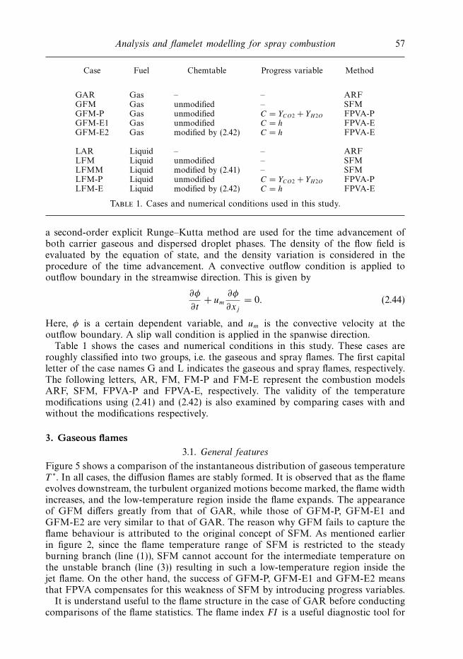
Figure 5 shows a comparison of the instantaneous distribution of gaseous temperatureT ∗. In all cases, the diffusion flames are stably formed. It is observed that as the flameevolves downstream, the turbulent organized motions become marked, the flame widthincreases, and the low-temperature region inside the flame expands. The appearanceof GFM differs greatly from that of GAR, while those of GFM-P, GFM-E1 andGFM-E2 are very similar to that of GAR. The reason why GFM fails to capture theflame behaviour is attributed to the original concept of SFM. As mentioned earlierin figure 2, since the flame temperature range of SFM is restricted to the steadyburning branch (line (1)), SFM cannot account for the intermediate temperature onthe unstable branch (line (3)) resulting in such a low-temperature region inside thejet flame. On the other hand, the success of GFM-P, GFM-E1 and GFM-E2 meansthat FPVA compensates for this weakness of SFM by introducing progress variables.
It is understand useful to the flame structure in the case of GAR before conductingcomparisons of the flame statistics. The flame index FI is a useful diagnostic tool for
58 Y. Baba and R. Kurose
(a)
(b) (c)
(d) (e)
1.0 8.3
Figure 5. Comparison of instantaneous distribution of gaseous temperature T ∗.(a) GAR, (b) GFM, (c) GFM-P, (d) GFM-E1 and (e) GFM-E2.
investigating the flame structure (Yamashita, Shimada & Takeno 1996). The value ofthe flame index is obtained by multiplying the spatial gradients of fuel and oxidizermass fractions as
FI = ∇YV · ∇YO, (3.1)
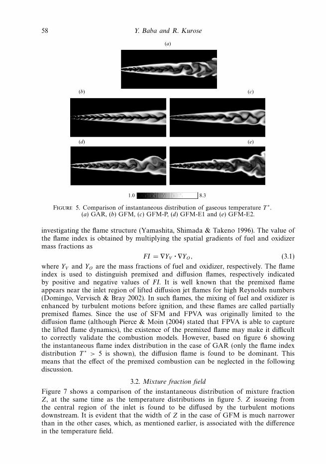
where YV and YO are the mass fractions of fuel and oxidizer, respectively. The flameindex is used to distinguish premixed and diffusion flames, respectively indicatedby positive and negative values of FI. It is well known that the premixed flameappears near the inlet region of lifted diffusion jet flames for high Reynolds numbers(Domingo, Vervisch & Bray 2002). In such flames, the mixing of fuel and oxidizer isenhanced by turbulent motions before ignition, and these flames are called partiallypremixed flames. Since the use of SFM and FPVA was originally limited to thediffusion flame (although Pierce & Moin (2004) stated that FPVA is able to capturethe lifted flame dynamics), the existence of the premixed flame may make it difficultto correctly validate the combustion models. However, based on figure 6 showingthe instantaneous flame index distribution in the case of GAR (only the flame indexdistribution T ∗ > 5 is shown), the diffusion flame is found to be dominant. Thismeans that the effect of the premixed combustion can be neglected in the followingdiscussion.
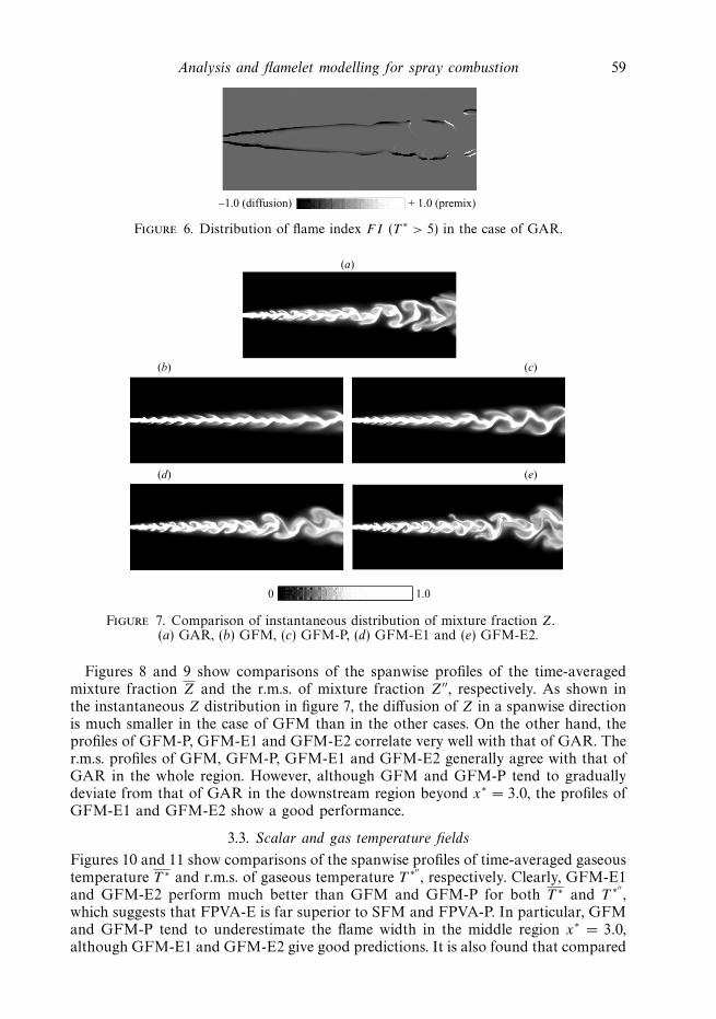
3.2. Mixture fraction field
Figure 7 shows a comparison of the instantaneous distribution of mixture fractionZ, at the same time as the temperature distributions in figure 5. Z issueing fromthe central region of the inlet is found to be diffused by the turbulent motionsdownstream. It is evident that the width of Z in the case of GFM is much narrowerthan in the other cases, which, as mentioned earlier, is associated with the differencein the temperature field.
Analysis and flamelet modelling for spray combustion 59
–1.0 (diffusion) + 1.0 (premix)
Figure 6. Distribution of flame index FI (T ∗ > 5) in the case of GAR.
(a)
(b) (c)
(d) (e)
0 1.0
Figure 7. Comparison of instantaneous distribution of mixture fraction Z.(a) GAR, (b) GFM, (c) GFM-P, (d) GFM-E1 and (e) GFM-E2.
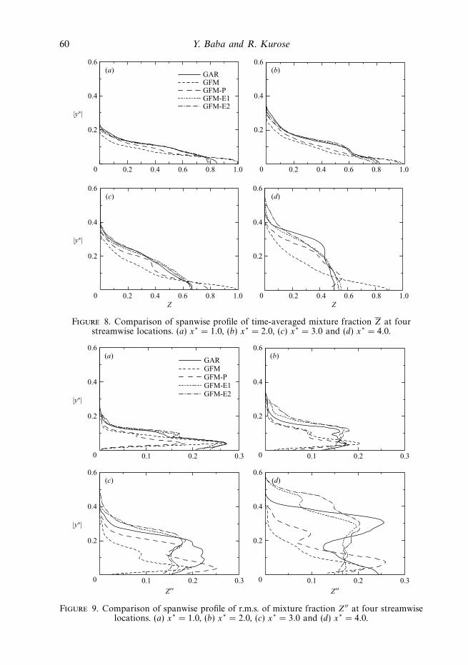
Figures 8 and 9 show comparisons of the spanwise profiles of the time-averagedmixture fraction Z and the r.m.s. of mixture fraction Z′′, respectively. As shown inthe instantaneous Z distribution in figure 7, the diffusion of Z in a spanwise directionis much smaller in the case of GFM than in the other cases. On the other hand, theprofiles of GFM-P, GFM-E1 and GFM-E2 correlate very well with that of GAR. Ther.m.s. profiles of GFM, GFM-P, GFM-E1 and GFM-E2 generally agree with that ofGAR in the whole region. However, although GFM and GFM-P tend to graduallydeviate from that of GAR in the downstream region beyond x∗ = 3.0, the profiles ofGFM-E1 and GFM-E2 show a good performance.
3.3. Scalar and gas temperature fields
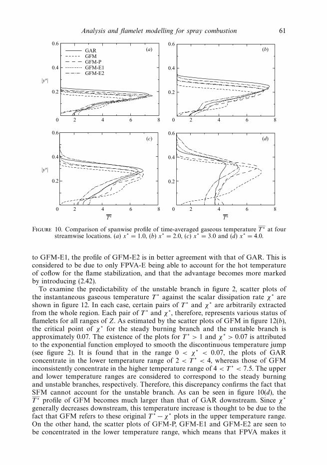
Figures 10 and 11 show comparisons of the spanwise profiles of time-averaged gaseoustemperature T ∗ and r.m.s. of gaseous temperature T ∗′′
, respectively. Clearly, GFM-E1and GFM-E2 perform much better than GFM and GFM-P for both T ∗ and T ∗′′
,which suggests that FPVA-E is far superior to SFM and FPVA-P. In particular, GFMand GFM-P tend to underestimate the flame width in the middle region x∗ = 3.0,although GFM-E1 and GFM-E2 give good predictions. It is also found that compared
60 Y. Baba and R. Kurose
0.6(a)
GARGFMGFM-PGFM-E1GFM-E2
0.4
|y∗|
0.2
0 0.2 0.4 0.6 0.8 1.0
0.6(b)
0.4
0.2
0 0.2 0.4 0.6 0.8 1.0
0.6(c)
0.4
|y∗|
0.2
0 0.2 0.4Z Z
0.6 0.8 1.0
0.6(d)
0.4
0.2
0 0.2 0.4 0.6 0.8 1.0
Figure 8. Comparison of spanwise profile of time-averaged mixture fraction Z at fourstreamwise locations. (a) x∗ = 1.0, (b) x∗ = 2.0, (c) x∗ = 3.0 and (d) x∗ = 4.0.
0.6(a)
GARGFMGFM-PGFM-E1GFM-E2
0.4
|y∗|
0.2
0.1 0.2 0.30
0.6(b)
0.4
0.2
0.1 0.2 0.30
0.6(c)
0.4
|y∗|
0.2
0.1 0.2
Z′′ Z′′0.30
0.6(d)
0.4
0.2
0.1 0.2 0.30
Figure 9. Comparison of spanwise profile of r.m.s. of mixture fraction Z′′ at four streamwiselocations. (a) x∗ = 1.0, (b) x∗ = 2.0, (c) x∗ = 3.0 and (d) x∗ = 4.0.
Analysis and flamelet modelling for spray combustion 61
0.6(a)GAR
GFMGFM-PGFM-E1GFM-E2
0.4
|y∗|
0.2
0 2 4 6 8
0.6(b)
0.4
0.2
0 2 4 6 8
0.6(c)
0.4
|y∗|
0.2
0 2 4 6 8
0.6(d)
0.4
0.2
0 2 4 6 8
T∗ T∗
Figure 10. Comparison of spanwise profile of time-averaged gaseous temperature T ∗ at fourstreamwise locations. (a) x∗ = 1.0, (b) x∗ = 2.0, (c) x∗ = 3.0 and (d) x∗ = 4.0.
to GFM-E1, the profile of GFM-E2 is in better agreement with that of GAR. This isconsidered to be due to only FPVA-E being able to account for the hot temperatureof coflow for the flame stabilization, and that the advantage becomes more markedby introducing (2.42).
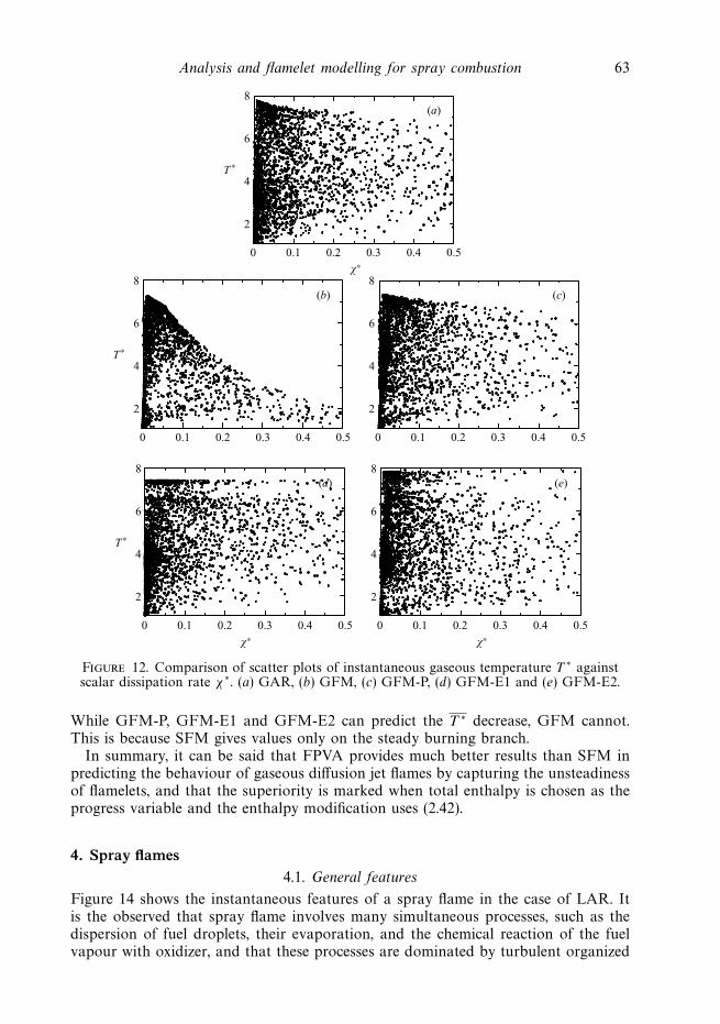
To examine the predictability of the unstable branch in figure 2, scatter plots ofthe instantaneous gaseous temperature T ∗ against the scalar dissipation rate χ∗ areshown in figure 12. In each case, certain pairs of T ∗ and χ∗ are arbitrarily extractedfrom the whole region. Each pair of T ∗ and χ∗, therefore, represents various status offlamelets for all ranges of Z. As estimated by the scatter plots of GFM in figure 12(b),the critical point of χ∗ for the steady burning branch and the unstable branch isapproximately 0.07. The existence of the plots for T ∗ > 1 and χ∗ > 0.07 is attributedto the exponential function employed to smooth the discontinuous temperature jump(see figure 2). It is found that in the range 0 < χ∗ < 0.07, the plots of GARconcentrate in the lower temperature range of 2 < T ∗ < 4, whereas those of GFMinconsistently concentrate in the higher temperature range of 4 < T ∗ < 7.5. The upperand lower temperature ranges are considered to correspond to the steady burningand unstable branches, respectively. Therefore, this discrepancy confirms the fact thatSFM cannot account for the unstable branch. As can be seen in figure 10(d), theT ∗ profile of GFM becomes much larger than that of GAR downstream. Since χ∗
generally decreases downstream, this temperature increase is thought to be due to thefact that GFM refers to these original T ∗ − χ∗ plots in the upper temperature range.On the other hand, the scatter plots of GFM-P, GFM-E1 and GFM-E2 are seen tobe concentrated in the lower temperature range, which means that FPVA makes it
62 Y. Baba and R. Kurose
0.6(a) GAR
GFMGFM-PGFM-E1GFM-E2
0.4
|y∗|
0.2
0 1 2 3
0.6(b)
0.4
0.2
0 1 2 3
0.6(c)
0.4
|y∗|
0.2
0 1 2
T∗′′ T∗′′3
0.6(d)
0.4
0.2
0 1 2 3
Figure 11. Comparison of spanwise profile of r.m.s. of gaseous temperature T ∗′′at four
streamwise locations. (a) x∗ = 1.0, (b) x∗ = 2.0, (c) x∗ = 3.0 and (d) x∗ = 4.0.
possible to simulate the flamelets on the unstable branch. Furthermore, in the case ofGFM-E2, the lower temperature range better correlates with that of GAR than theother cases. In addition, the higher temperature plots located up to T ∗ = 8 can becaptured, which shows the validity of the enthalpy modification procedure using (2.42).
It is also found that the plots of GAR, GFM-P, GFM-E1 and GFM-E2 aredistributed in the wide range of 0 < χ∗ < 0.5 and 1 < T ∗ < 8 illustrated, whereasthose of GFM are non-existent high χ∗ and high T ∗, despite employing an exponentialfunction to smooth the discontinuous temperature jump. The plots in this rangeoriginate from the high-temperature coflow issuing from the inlet to ignite the flame.The reason why GFM-P, GFM-E1 and GFM-E2 can give results in this range is thatχ∗ is represented in FPVA. In other words, FPVA has the ability to capture the effectof ignition by the high-temperature coflow.
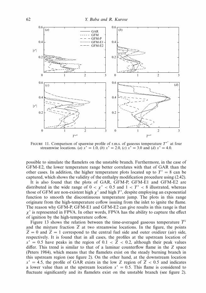
Figure 13 shows the relation between the time-averaged gaseous temperature T ∗
and the mixture fraction Z at two streamwise locations. In the figure, the pointsZ = 0 and Z = 1 correspond to the central fuel side and outer oxidizer (air) side,respectively. It is found that in all cases, the profiles at the upstream location ofx∗ = 0.5 have peaks in the region of 0.1 < Z < 0.2, although their peak valuesdiffer. This trend is similar to that of a laminar counterflow flame in the Z space(Peters 1984), which means that the flamelets exist on the steady burning branch inthis upstream region (see figure 2). On the other hand, at the downstream locationx∗ = 4.5, the profile of GAR exists in the low Z region of Z < 0.5 and indicatesa lower value than at the upstream location x∗ = 0.5. This flame is considered tofluctuate significantly and its flamelets exist on the unstable branch (see figure 2).
Analysis and flamelet modelling for spray combustion 63
8(a)
6
T∗
χ∗
χ∗ χ∗
4
2
0 0.1 0.2 0.3 0.4 0.5
8(b)
6
T∗
4
2
0 0.1 0.2 0.3 0.4 0.5
8(c)
6
4
2
0 0.1 0.2 0.3 0.4 0.5
8(d)
6
T∗
4
2
0 0.1 0.2 0.3 0.4 0.5
8(e)
6
4
2
0 0.1 0.2 0.3 0.4 0.5
Figure 12. Comparison of scatter plots of instantaneous gaseous temperature T ∗ againstscalar dissipation rate χ∗. (a) GAR, (b) GFM, (c) GFM-P, (d) GFM-E1 and (e) GFM-E2.
While GFM-P, GFM-E1 and GFM-E2 can predict the T ∗ decrease, GFM cannot.This is because SFM gives values only on the steady burning branch.
In summary, it can be said that FPVA provides much better results than SFM inpredicting the behaviour of gaseous diffusion jet flames by capturing the unsteadinessof flamelets, and that the superiority is marked when total enthalpy is chosen as theprogress variable and the enthalpy modification uses (2.42).
4. Spray flames4.1. General features
Figure 14 shows the instantaneous features of a spray flame in the case of LAR. Itis the observed that spray flame involves many simultaneous processes, such as thedispersion of fuel droplets, their evaporation, and the chemical reaction of the fuelvapour with oxidizer, and that these processes are dominated by turbulent organized
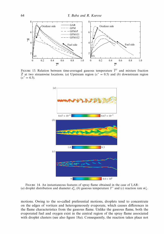
64 Y. Baba and R. Kurose
8
Oxidizer side
Fuel side
GARGFMGFM-PGFM-E1GFM-E2
6
4
2
0
(a)
0.2 0.4 0.6 0.8 1.0
Z∗
8
Oxidizer side
Fuel side
6
4
2
0
(b)
0.2 0.4 0.6 0.8 1.0
Z∗
T∗
Figure 13. Relation between time-averaged gaseous temperature T ∗ and mixture fractionZ at two streamwise locations. (a) Upstream region (x∗ = 0.5) and (b) downstream region(x∗ = 4.5).
(a)
(b)
(c)
0.67 × 10⁻⁴ 0.67 × 10⁻³
4.0 × 10⁶
1.0 8.3
0
Figure 14. An instantaneous features of spray flame obtained in the case of LAR:(a) droplet distribution and diameter d∗
d , (b) gaseous temperature T ∗ and (c) reaction rate m∗V .
motions. Owing to the so-called preferential motions, droplets tend to concentrateon the edges of vortices and heterogeneously evaporate, which causes differences inthe flame characteristics from the gaseous flame. Unlike the gaseous flame, both theevaporated fuel and oxygen exist in the central region of the spray flame associatedwith droplet clusters (see also figure 18a). Consequently, the reaction takes place not
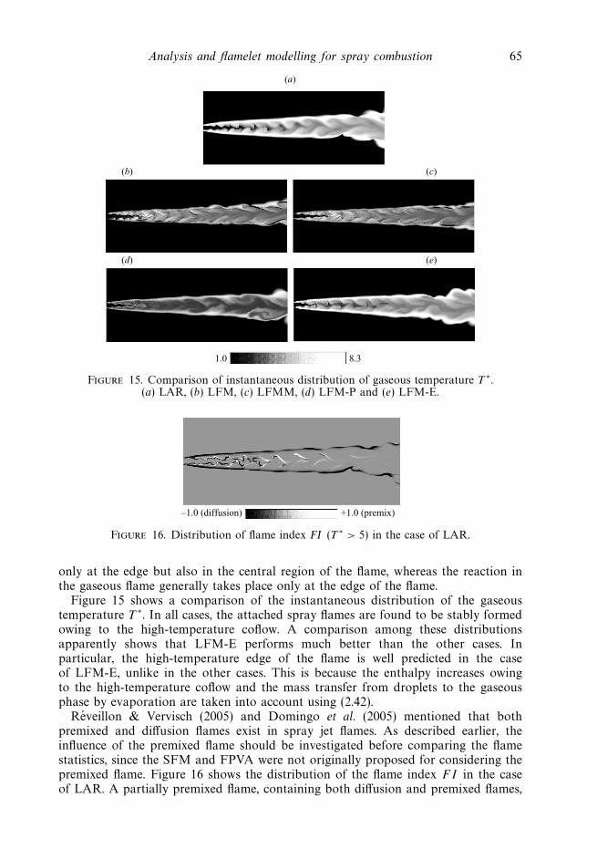
Analysis and flamelet modelling for spray combustion 65
(a)
(b) (c)
(d) (e)
1.0 8.3
Figure 15. Comparison of instantaneous distribution of gaseous temperature T ∗.(a) LAR, (b) LFM, (c) LFMM, (d) LFM-P and (e) LFM-E.
–1.0 (diffusion) +1.0 (premix)
Figure 16. Distribution of flame index FI (T ∗ > 5) in the case of LAR.
only at the edge but also in the central region of the flame, whereas the reaction inthe gaseous flame generally takes place only at the edge of the flame.
Figure 15 shows a comparison of the instantaneous distribution of the gaseoustemperature T ∗. In all cases, the attached spray flames are found to be stably formedowing to the high-temperature coflow. A comparison among these distributionsapparently shows that LFM-E performs much better than the other cases. Inparticular, the high-temperature edge of the flame is well predicted in the caseof LFM-E, unlike in the other cases. This is because the enthalpy increases owingto the high-temperature coflow and the mass transfer from droplets to the gaseousphase by evaporation are taken into account using (2.42).
Reveillon & Vervisch (2005) and Domingo et al. (2005) mentioned that bothpremixed and diffusion flames exist in spray jet flames. As described earlier, theinfluence of the premixed flame should be investigated before comparing the flamestatistics, since the SFM and FPVA were not originally proposed for considering thepremixed flame. Figure 16 shows the distribution of the flame index FI in the caseof LAR. A partially premixed flame, containing both diffusion and premixed flames,
66 Y. Baba and R. Kurose
0.3
0.2
Pp (x∗)
0.1
0 1 2 3 4 5
x∗
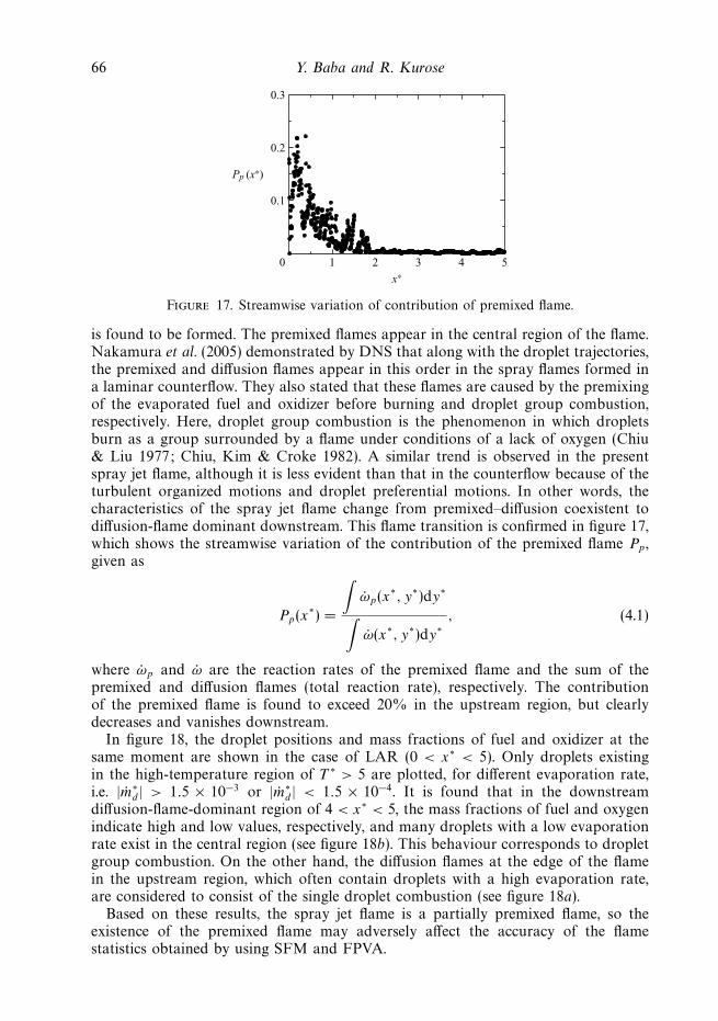
Figure 17. Streamwise variation of contribution of premixed flame.
is found to be formed. The premixed flames appear in the central region of the flame.Nakamura et al. (2005) demonstrated by DNS that along with the droplet trajectories,the premixed and diffusion flames appear in this order in the spray flames formed ina laminar counterflow. They also stated that these flames are caused by the premixingof the evaporated fuel and oxidizer before burning and droplet group combustion,respectively. Here, droplet group combustion is the phenomenon in which dropletsburn as a group surrounded by a flame under conditions of a lack of oxygen (Chiu& Liu 1977; Chiu, Kim & Croke 1982). A similar trend is observed in the presentspray jet flame, although it is less evident than that in the counterflow because of theturbulent organized motions and droplet preferential motions. In other words, thecharacteristics of the spray jet flame change from premixed–diffusion coexistent todiffusion-flame dominant downstream. This flame transition is confirmed in figure 17,which shows the streamwise variation of the contribution of the premixed flame Pp ,given as
Pp(x∗) =
∫ωp(x∗, y∗)dy∗
∫ω(x∗, y∗)dy∗
, (4.1)
where ωp and ω are the reaction rates of the premixed flame and the sum of thepremixed and diffusion flames (total reaction rate), respectively. The contributionof the premixed flame is found to exceed 20% in the upstream region, but clearlydecreases and vanishes downstream.
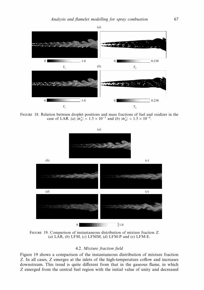
In figure 18, the droplet positions and mass fractions of fuel and oxidizer at thesame moment are shown in the case of LAR (0 < x∗ < 5). Only droplets existingin the high-temperature region of T ∗ > 5 are plotted, for different evaporation rate,i.e. |m∗
d | > 1.5 × 10⁻³ or |m∗d | < 1.5 × 10⁻⁴. It is found that in the downstream
diffusion-flame-dominant region of 4 < x∗ < 5, the mass fractions of fuel and oxygenindicate high and low values, respectively, and many droplets with a low evaporationrate exist in the central region (see figure 18b). This behaviour corresponds to dropletgroup combustion. On the other hand, the diffusion flames at the edge of the flamein the upstream region, which often contain droplets with a high evaporation rate,are considered to consist of the single droplet combustion (see figure 18a).
Based on these results, the spray jet flame is a partially premixed flame, so theexistence of the premixed flame may adversely affect the accuracy of the flamestatistics obtained by using SFM and FPVA.
Analysis and flamelet modelling for spray combustion 67
(a)
(b)
0 1.0
Yv Yo
0 0.238
0 1.0
Yv Yo
0 0.238
Figure 18. Relation between droplet positions and mass fractions of fuel and oxidizer in thecase of LAR. (a) |m∗
d | > 1.5 × 10⁻³ and (b) |m∗d | < 1.5 × 10⁻⁴.
(a)
(b) (c)
(d) (e)
0 1.0
Figure 19. Comparison of instantaneous distribution of mixture fraction Z.(a) LAR, (b) LFM, (c) LFMM, (d) LFM-P and (e) LFM-E.
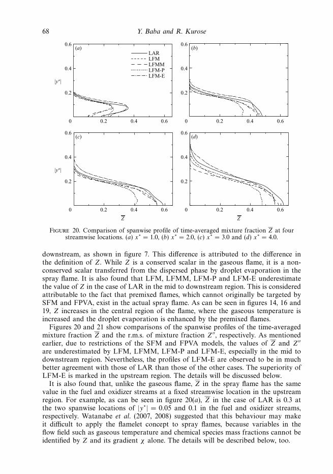
4.2. Mixture fraction field
Figure 19 shows a comparison of the instantaneous distribution of mixture fractionZ. In all cases, Z emerges at the inlets of the high-temperature coflow and increasesdownstream. This trend is quite different from that in the gaseous flame, in whichZ emerged from the central fuel region with the initial value of unity and decreased
68 Y. Baba and R. Kurose
0.6
LARLFMLFMMLFM-PLFM-E
0.4
0.2
0 0.2 0.4 0.6
(a)0.6
0.4
0.2
0 0.2 0.4 0.6
(b)
|y∗|
0.6
0.4
0.2
0 0.2 0.4 0.6
(c)0.6
0.4
0.2
0 0.2 0.4 0.6
(d)
|y∗|
Z Z
Figure 20. Comparison of spanwise profile of time-averaged mixture fraction Z at fourstreamwise locations. (a) x∗ = 1.0, (b) x∗ = 2.0, (c) x∗ = 3.0 and (d) x∗ = 4.0.
downstream, as shown in figure 7. This difference is attributed to the difference inthe definition of Z. While Z is a conserved scalar in the gaseous flame, it is a non-conserved scalar transferred from the dispersed phase by droplet evaporation in thespray flame. It is also found that LFM, LFMM, LFM-P and LFM-E underestimatethe value of Z in the case of LAR in the mid to downstream region. This is consideredattributable to the fact that premixed flames, which cannot originally be targeted bySFM and FPVA, exist in the actual spray flame. As can be seen in figures 14, 16 and19, Z increases in the central region of the flame, where the gaseous temperature isincreased and the droplet evaporation is enhanced by the premixed flames.
Figures 20 and 21 show comparisons of the spanwise profiles of the time-averagedmixture fraction Z and the r.m.s. of mixture fraction Z′′, respectively. As mentionedearlier, due to restrictions of the SFM and FPVA models, the values of Z and Z′′
are underestimated by LFM, LFMM, LFM-P and LFM-E, especially in the mid todownstream region. Nevertheless, the profiles of LFM-E are observed to be in muchbetter agreement with those of LAR than those of the other cases. The superiority ofLFM-E is marked in the upstream region. The details will be discussed below.
It is also found that, unlike the gaseous flame, Z in the spray flame has the samevalue in the fuel and oxidizer streams at a fixed streamwise location in the upstreamregion. For example, as can be seen in figure 20(a), Z in the case of LAR is 0.3 atthe two spanwise locations of |y∗| = 0.05 and 0.1 in the fuel and oxidizer streams,respectively. Watanabe et al. (2007, 2008) suggested that this behaviour may makeit difficult to apply the flamelet concept to spray flames, because variables in theflow field such as gaseous temperature and chemical species mass fractions cannot beidentified by Z and its gradient χ alone. The details will be described below, too.
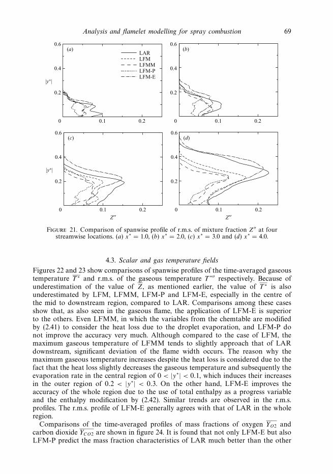
Analysis and flamelet modelling for spray combustion 69
0.6(a)
LARLFMLFMMLFM-PLFM-E
0.4
0.2
0 0.1 0.2
0.6(b)
0.4
0.2
0 0.1 0.2
|y∗|
0.6(c)
0.4
0.2
0 0.1
Z′′ Z′′0.2
0.6(d)
0.4
0.2
0 0.1 0.2
|y∗|
Figure 21. Comparison of spanwise profile of r.m.s. of mixture fraction Z′′ at fourstreamwise locations. (a) x∗ = 1.0, (b) x∗ = 2.0, (c) x∗ = 3.0 and (d) x∗ = 4.0.
4.3. Scalar and gas temperature fields
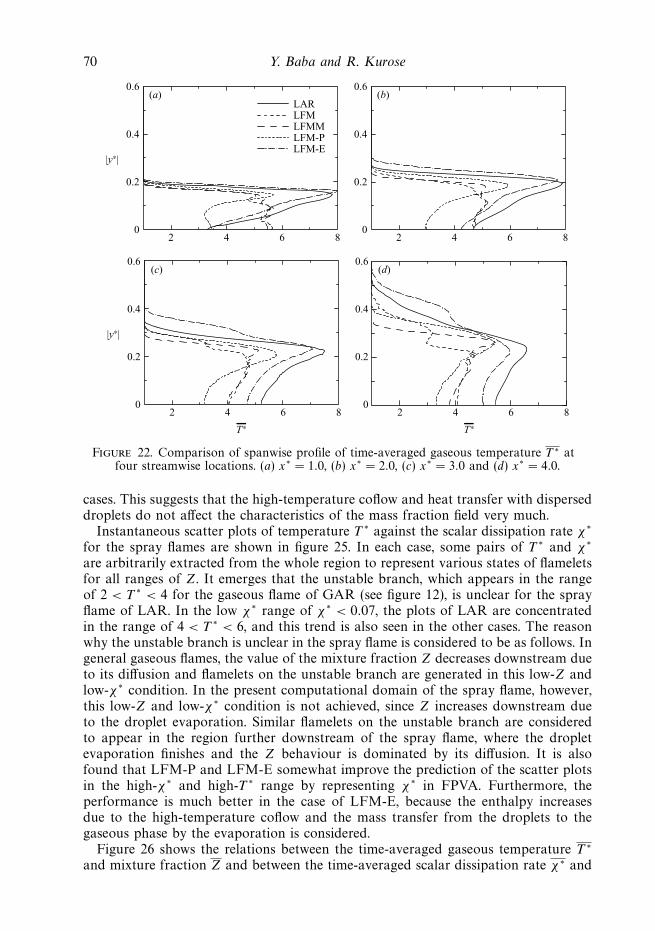
Figures 22 and 23 show comparisons of spanwise profiles of the time-averaged gaseoustemperature T ∗ and r.m.s. of the gaseous temperature T ∗′′ respectively. Because ofunderestimation of the value of Z, as mentioned earlier, the value of T ∗ is alsounderestimated by LFM, LFMM, LFM-P and LFM-E, especially in the centre ofthe mid to downstream region, compared to LAR. Comparisons among these casesshow that, as also seen in the gaseous flame, the application of LFM-E is superiorto the others. Even LFMM, in which the variables from the chemtable are modifiedby (2.41) to consider the heat loss due to the droplet evaporation, and LFM-P donot improve the accuracy very much. Although compared to the case of LFM, themaximum gaseous temperature of LFMM tends to slightly approach that of LARdownstream, significant deviation of the flame width occurs. The reason why themaximum gaseous temperature increases despite the heat loss is considered due to thefact that the heat loss slightly decreases the gaseous temperature and subsequently theevaporation rate in the central region of 0 < |y∗| < 0.1, which induces their increasesin the outer region of 0.2 < |y∗| < 0.3. On the other hand, LFM-E improves theaccuracy of the whole region due to the use of total enthalpy as a progress variableand the enthalpy modification by (2.42). Similar trends are observed in the r.m.s.profiles. The r.m.s. profile of LFM-E generally agrees with that of LAR in the wholeregion.
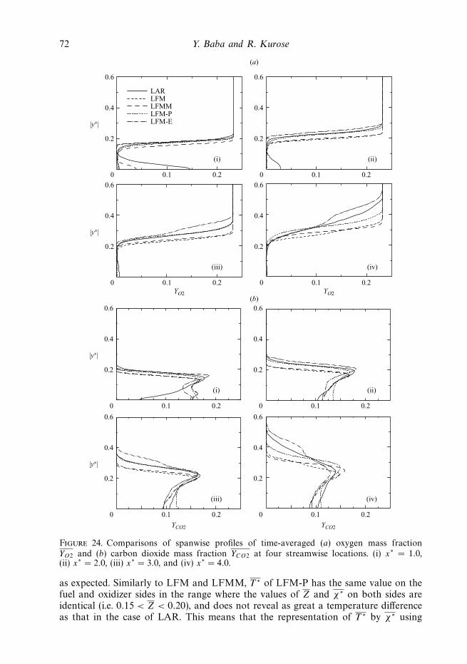
Comparisons of the time-averaged profiles of mass fractions of oxygen YO2 andcarbon dioxide YCO2 are shown in figure 24. It is found that not only LFM-E but alsoLFM-P predict the mass fraction characteristics of LAR much better than the other
70 Y. Baba and R. Kurose
0.6
LARLFMLFMMLFM-PLFM-E
0.4
0.2
2 4 6 80
(a)0.6
0.4
0.2
2 4 6 80
(b)
|y∗|
0.6
0.4
0.2
2 4 6 80
(c)0.6
0.4
0.2
2 4 6 80
(d)
|y∗|
T∗ T∗
Figure 22. Comparison of spanwise profile of time-averaged gaseous temperature T ∗ atfour streamwise locations. (a) x∗ = 1.0, (b) x∗ = 2.0, (c) x∗ = 3.0 and (d) x∗ = 4.0.
cases. This suggests that the high-temperature coflow and heat transfer with disperseddroplets do not affect the characteristics of the mass fraction field very much.
Instantaneous scatter plots of temperature T ∗ against the scalar dissipation rate χ∗
for the spray flames are shown in figure 25. In each case, some pairs of T ∗ and χ∗
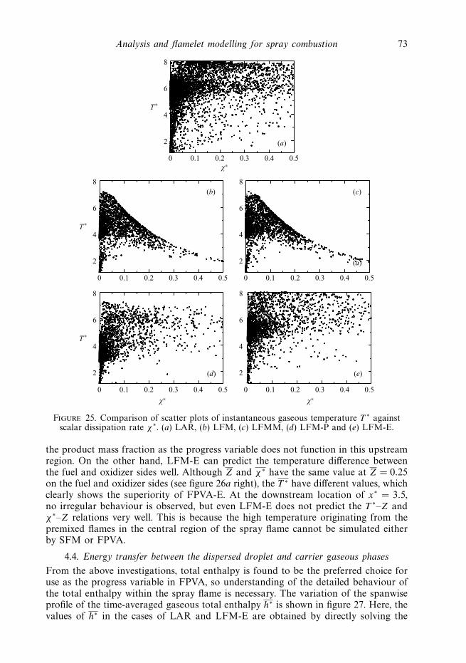
are arbitrarily extracted from the whole region to represent various states of flameletsfor all ranges of Z. It emerges that the unstable branch, which appears in the rangeof 2 < T ∗ < 4 for the gaseous flame of GAR (see figure 12), is unclear for the sprayflame of LAR. In the low χ∗ range of χ∗ < 0.07, the plots of LAR are concentratedin the range of 4 < T ∗ < 6, and this trend is also seen in the other cases. The reasonwhy the unstable branch is unclear in the spray flame is considered to be as follows. Ingeneral gaseous flames, the value of the mixture fraction Z decreases downstream dueto its diffusion and flamelets on the unstable branch are generated in this low-Z andlow-χ∗ condition. In the present computational domain of the spray flame, however,this low-Z and low-χ∗ condition is not achieved, since Z increases downstream dueto the droplet evaporation. Similar flamelets on the unstable branch are consideredto appear in the region further downstream of the spray flame, where the dropletevaporation finishes and the Z behaviour is dominated by its diffusion. It is alsofound that LFM-P and LFM-E somewhat improve the prediction of the scatter plotsin the high-χ∗ and high-T ∗ range by representing χ∗ in FPVA. Furthermore, theperformance is much better in the case of LFM-E, because the enthalpy increasesdue to the high-temperature coflow and the mass transfer from the droplets to thegaseous phase by the evaporation is considered.
Figure 26 shows the relations between the time-averaged gaseous temperature T ∗
and mixture fraction Z and between the time-averaged scalar dissipation rate χ∗ and
Analysis and flamelet modelling for spray combustion 71
0.6
LARLFMLFMMLFM-PLFM-E
0.4
0.2
0 1 2 3 4
(a)0.6
0.4
0.2
0 1 2 3 4
(b)
|y∗|
0.6
0.4
0.2
0 1 2 3 4
(c)0.6
0.4
0.2
0 1 2 3 4
(d)
|y∗|
T∗′′ T∗′′
Figure 23. Comparison of spanwise profile of r.m.s. of gaseous temperature T ∗′′ at fourstreamwise locations. (a) x∗ = 1.0, (b) x∗ = 2.0, (c) x∗ = 3.0 and (d) x∗ = 4.0.
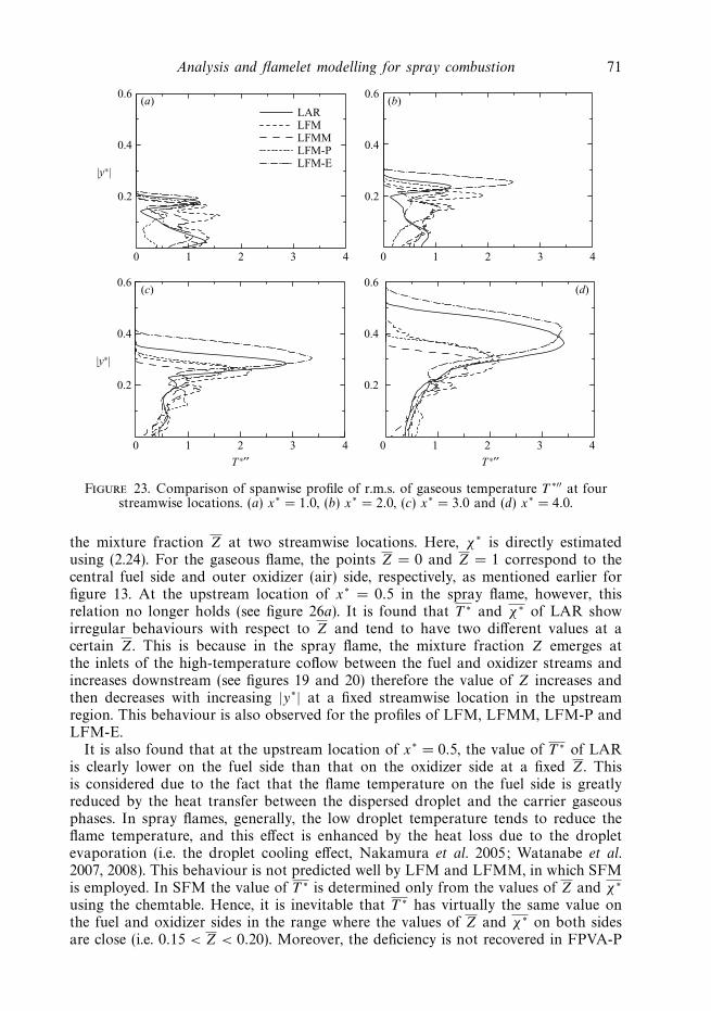
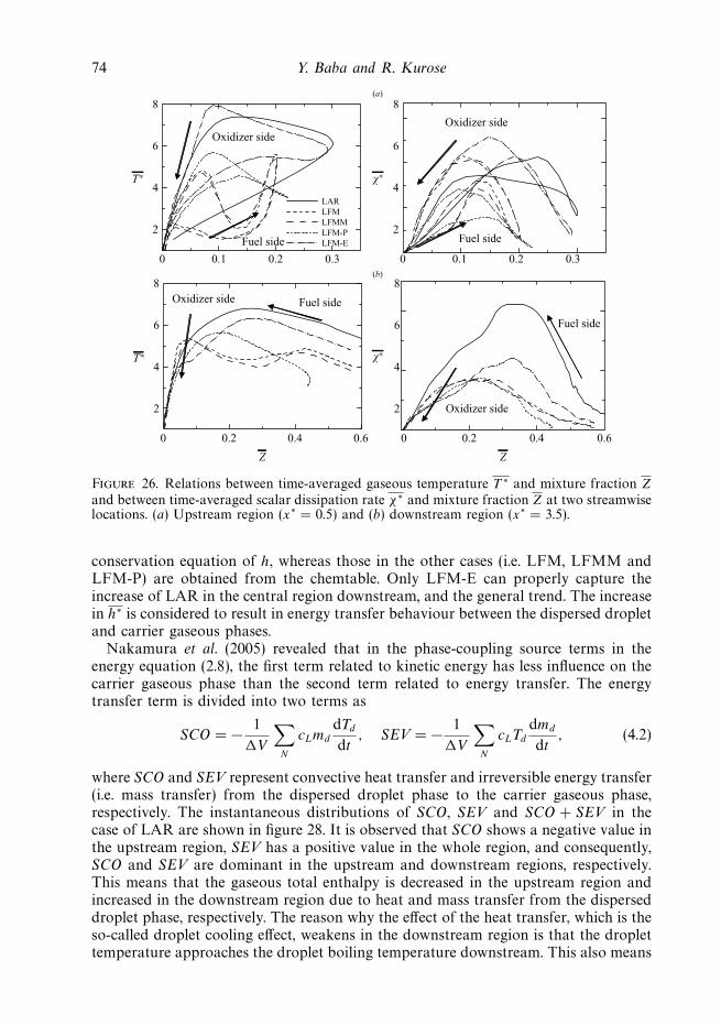
the mixture fraction Z at two streamwise locations. Here, χ∗ is directly estimatedusing (2.24). For the gaseous flame, the points Z = 0 and Z = 1 correspond to thecentral fuel side and outer oxidizer (air) side, respectively, as mentioned earlier forfigure 13. At the upstream location of x∗ = 0.5 in the spray flame, however, thisrelation no longer holds (see figure 26a). It is found that T ∗ and χ∗ of LAR showirregular behaviours with respect to Z and tend to have two different values at acertain Z. This is because in the spray flame, the mixture fraction Z emerges atthe inlets of the high-temperature coflow between the fuel and oxidizer streams andincreases downstream (see figures 19 and 20) therefore the value of Z increases andthen decreases with increasing |y∗| at a fixed streamwise location in the upstreamregion. This behaviour is also observed for the profiles of LFM, LFMM, LFM-P andLFM-E.
It is also found that at the upstream location of x∗ = 0.5, the value of T ∗ of LARis clearly lower on the fuel side than that on the oxidizer side at a fixed Z. Thisis considered due to the fact that the flame temperature on the fuel side is greatlyreduced by the heat transfer between the dispersed droplet and the carrier gaseousphases. In spray flames, generally, the low droplet temperature tends to reduce theflame temperature, and this effect is enhanced by the heat loss due to the dropletevaporation (i.e. the droplet cooling effect, Nakamura et al. 2005; Watanabe et al.2007, 2008). This behaviour is not predicted well by LFM and LFMM, in which SFMis employed. In SFM the value of T ∗ is determined only from the values of Z and χ∗
using the chemtable. Hence, it is inevitable that T ∗ has virtually the same value onthe fuel and oxidizer sides in the range where the values of Z and χ∗ on both sidesare close (i.e. 0.15 < Z < 0.20). Moreover, the deficiency is not recovered in FPVA-P
72 Y. Baba and R. Kurose
0.6
LARLFMLFMMLFM-PLFM-E
0.4
0.2
0 0.1 0.2
0.6
0.4
0.2
0 0.1
YO2
YCO2 YCO2
YO2
0.2
(i) (ii)
(a)
(b)
|y∗|
0.6
0.4
0.2
0 0.1 0.2
0.6
0.4
0.2
0 0.1 0.2
(iii) (iv)
|y∗|
0.6
0.4
0.2
0 0.1 0.2
0.6
0.4
0.2
0 0.1 0.2
(i) (ii)
|y∗|
0.6
0.4
0.2
0 0.1 0.2
0.6
0.4
0.2
0 0.1 0.2
(iii) (iv)
|y∗|
Figure 24. Comparisons of spanwise profiles of time-averaged (a) oxygen mass fractionYO2 and (b) carbon dioxide mass fraction YCO2 at four streamwise locations. (i) x∗ = 1.0,(ii) x∗ = 2.0, (iii) x∗ = 3.0, and (iv) x∗ = 4.0.
as expected. Similarly to LFM and LFMM, T ∗ of LFM-P has the same value on thefuel and oxidizer sides in the range where the values of Z and χ∗ on both sides areidentical (i.e. 0.15 < Z < 0.20), and does not reveal as great a temperature differenceas that in the case of LAR. This means that the representation of T ∗ by χ∗ using
Analysis and flamelet modelling for spray combustion 73
8
6
4
2
0 0.1 0.2 0.3 0.4 0.5
(a)
T∗
8
6
4
2
0 0.1 0.2 0.3 0.4 0.5
(b) (c)
T∗
8
6
4
2
0 0.1 0.2 0.3 0.4 0.5
8
6
4
2
0 0.1 0.2 0.3 0.4 0.5
(d) (e)
T∗
8
6
4
2
0 0.1 0.2 0.3 0.4 0.5
(a)
χ∗ χ∗
χ∗
Figure 25. Comparison of scatter plots of instantaneous gaseous temperature T ∗ againstscalar dissipation rate χ∗. (a) LAR, (b) LFM, (c) LFMM, (d) LFM-P and (e) LFM-E.
the product mass fraction as the progress variable does not function in this upstreamregion. On the other hand, LFM-E can predict the temperature difference betweenthe fuel and oxidizer sides well. Although Z and χ∗ have the same value at Z = 0.25on the fuel and oxidizer sides (see figure 26a right), the T ∗ have different values, whichclearly shows the superiority of FPVA-E. At the downstream location of x∗ = 3.5,no irregular behaviour is observed, but even LFM-E does not predict the T ∗–Z andχ∗–Z relations very well. This is because the high temperature originating from thepremixed flames in the central region of the spray flame cannot be simulated eitherby SFM or FPVA.
4.4. Energy transfer between the dispersed droplet and carrier gaseous phases
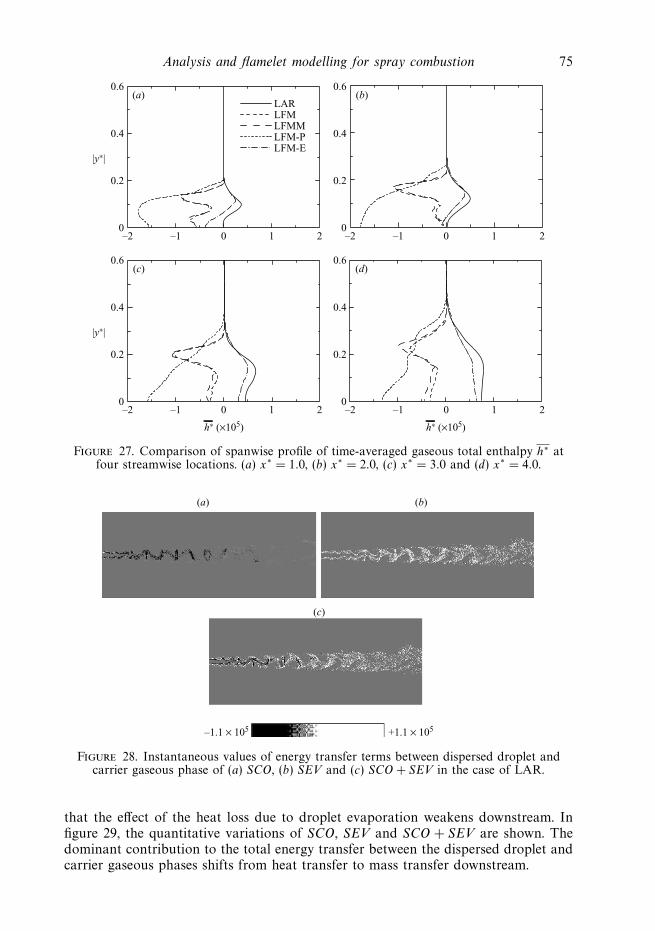
From the above investigations, total enthalpy is found to be the preferred choice foruse as the progress variable in FPVA, so understanding of the detailed behaviour ofthe total enthalpy within the spray flame is necessary. The variation of the spanwiseprofile of the time-averaged gaseous total enthalpy h∗ is shown in figure 27. Here, thevalues of h∗ in the cases of LAR and LFM-E are obtained by directly solving the
74 Y. Baba and R. Kurose
8
Oxidizer side
Oxidizer side
Oxidizer side
Oxidizer side
Fuel side
Fuel side
Fuel side
Fuel side
6
4
2
0 0.1 0.2 0.3
LAR
(a)
(b)
LFMLFMMLFM-PLFM-E
T∗ χ∗
χ∗
8
6
4
2
0 0.1 0.2 0.3
8
6
4
2
0 0.2 0.4 0.6 0.2 0.4 0.6
T∗
8
6
4
2
0
Z Z
Figure 26. Relations between time-averaged gaseous temperature T ∗ and mixture fraction Z
and between time-averaged scalar dissipation rate χ∗ and mixture fraction Z at two streamwiselocations. (a) Upstream region (x∗ = 0.5) and (b) downstream region (x∗ = 3.5).
conservation equation of h, whereas those in the other cases (i.e. LFM, LFMM andLFM-P) are obtained from the chemtable. Only LFM-E can properly capture theincrease of LAR in the central region downstream, and the general trend. The increasein h∗ is considered to result in energy transfer behaviour between the dispersed dropletand carrier gaseous phases.
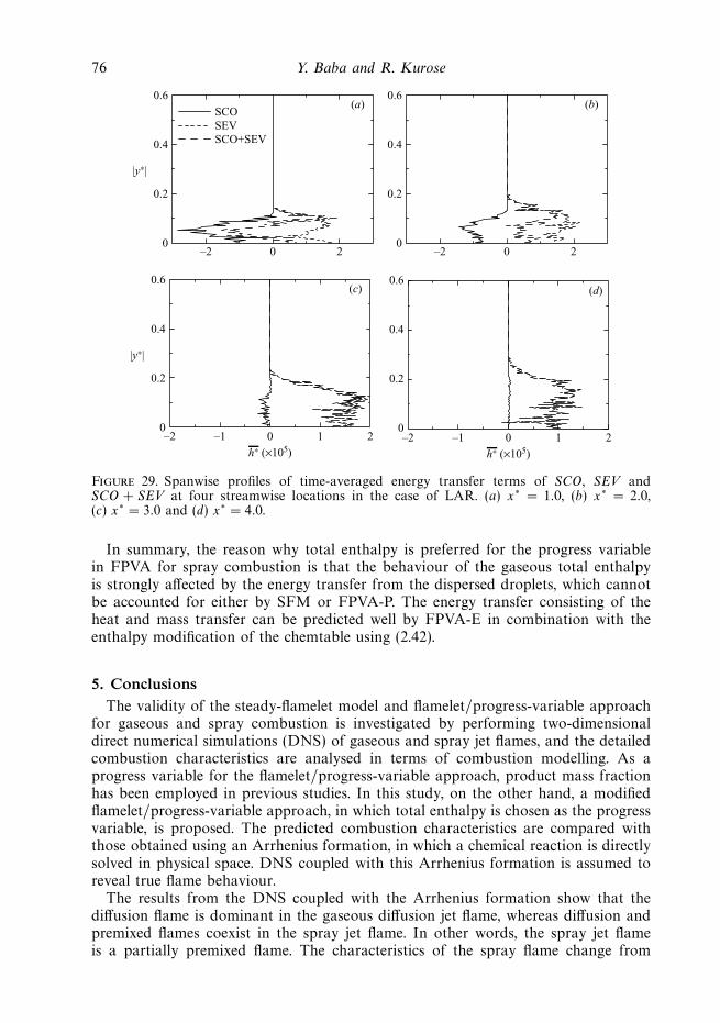
Nakamura et al. (2005) revealed that in the phase-coupling source terms in theenergy equation (2.8), the first term related to kinetic energy has less influence on thecarrier gaseous phase than the second term related to energy transfer. The energytransfer term is divided into two terms as
SCO = − 1
�V
∑N
cLmd
dTd
dt, SEV = − 1
�V
∑N
cLTd
dmd
dt, (4.2)
where SCO and SEV represent convective heat transfer and irreversible energy transfer(i.e. mass transfer) from the dispersed droplet phase to the carrier gaseous phase,respectively. The instantaneous distributions of SCO, SEV and SCO + SEV in thecase of LAR are shown in figure 28. It is observed that SCO shows a negative value inthe upstream region, SEV has a positive value in the whole region, and consequently,SCO and SEV are dominant in the upstream and downstream regions, respectively.This means that the gaseous total enthalpy is decreased in the upstream region andincreased in the downstream region due to heat and mass transfer from the disperseddroplet phase, respectively. The reason why the effect of the heat transfer, which is theso-called droplet cooling effect, weakens in the downstream region is that the droplettemperature approaches the droplet boiling temperature downstream. This also means
Analysis and flamelet modelling for spray combustion 75
0.6
LARLFMLFMMLFM-PLFM-E
0.4
0.2
0–2 –1 0 1 2
0.6
0.4
0.2
0–2 –1 0 1 2
(a) (b)
|y∗|
0.6
0.4
0.2
0–2 –1 0 1 2
0.6
0.4
0.2
0–2 –1 0 1 2
(c) (d)
|y∗|
h∗ (×105) h∗ (×105)
Figure 27. Comparison of spanwise profile of time-averaged gaseous total enthalpy h∗ atfour streamwise locations. (a) x∗ = 1.0, (b) x∗ = 2.0, (c) x∗ = 3.0 and (d) x∗ = 4.0.
(a) (b)
(c)
–1.1 × 10⁵ +1.1 × 10⁵
Figure 28. Instantaneous values of energy transfer terms between dispersed droplet andcarrier gaseous phase of (a) SCO, (b) SEV and (c) SCO + SEV in the case of LAR.
that the effect of the heat loss due to droplet evaporation weakens downstream. Infigure 29, the quantitative variations of SCO, SEV and SCO + SEV are shown. Thedominant contribution to the total energy transfer between the dispersed droplet andcarrier gaseous phases shifts from heat transfer to mass transfer downstream.
76 Y. Baba and R. Kurose
SCOSEVSCO+SEV
0.6
0.4
0.2
0–2 0 2
(a)0.6
0.4
0.2
0–2 0 2
(b)
|y∗|
0.6
0.4
0.2
0
(c)0.6
0.4
0.2
0
(d)
|y∗|
–2 –1 0 1 2
h∗ (×105)–2 –1 0 1 2
h∗ (×105)
Figure 29. Spanwise profiles of time-averaged energy transfer terms of SCO, SEV andSCO + SEV at four streamwise locations in the case of LAR. (a) x∗ = 1.0, (b) x∗ = 2.0,(c) x∗ = 3.0 and (d) x∗ = 4.0.
In summary, the reason why total enthalpy is preferred for the progress variablein FPVA for spray combustion is that the behaviour of the gaseous total enthalpyis strongly affected by the energy transfer from the dispersed droplets, which cannotbe accounted for either by SFM or FPVA-P. The energy transfer consisting of theheat and mass transfer can be predicted well by FPVA-E in combination with theenthalpy modification of the chemtable using (2.42).
5. ConclusionsThe validity of the steady-flamelet model and flamelet/progress-variable approach
for gaseous and spray combustion is investigated by performing two-dimensionaldirect numerical simulations (DNS) of gaseous and spray jet flames, and the detailedcombustion characteristics are analysed in terms of combustion modelling. As aprogress variable for the flamelet/progress-variable approach, product mass fractionhas been employed in previous studies. In this study, on the other hand, a modifiedflamelet/progress-variable approach, in which total enthalpy is chosen as the progressvariable, is proposed. The predicted combustion characteristics are compared withthose obtained using an Arrhenius formation, in which a chemical reaction is directlysolved in physical space. DNS coupled with this Arrhenius formation is assumed toreveal true flame behaviour.
The results from the DNS coupled with the Arrhenius formation show that thediffusion flame is dominant in the gaseous diffusion jet flame, whereas diffusion andpremixed flames coexist in the spray jet flame. In other words, the spray jet flameis a partially premixed flame. The characteristics of the spray flame change from
Analysis and flamelet modelling for spray combustion 77
premixed–diffusion coexistent to diffusion-flame dominant downstream, and dropletgroup combustion appears in the diffusion-flame-dominant region. It is also foundthat although the flamelets on the unstable branch, which indicate low temperatureunder conditions of low mixture fraction and low scalar dissipation rate, are formedin the downstream region of the gaseous flame, they hardly appear in the spraycombustion. This is because the mixture fraction of the spray flame tends to increasedownstream.
Comparisons with the DNS results coupled with the steady-flamelet modeland flamelet/progress-variable approach show that the flamelet/progress-variableapproach, in which total enthalpy is employed as the progress variable, is superior tothe other combustion models, and that this superiority is remarkable for the sprayflame. This is because the behaviour of the gaseous total enthalpy is strongly affectedby the energy transfer (i.e. heat transfer and mass transfer) from the dispersed droplet,and this effect can be accounted for only by solving the conservation equation of thetotal enthalpy.
It is also found that even using DNS with the flamelet/progress-variable approachemploying the total enthalpy as the progress variable, the characteristics of thepremixed flame appearing in the central region of the spray jet flame cannot be wellpredicted. The predicted gaseous temperature is underestimated in this region. Thissuggests that the combustion model for the partially premixed flame is necessary forthe spray flame. In addition, the flamelets on the unstable branch are consideredto appear in the region further downstream of the spray flame. The behaviour andthe validity of the present flamelet/progress-variable approach in this region are stillopen to question.
The authors would like to thank Professor Fumiteru Akamatsu of Osaka Universityand Dr Hiroaki Watanabe of CRIEPI for their useful discussion. R.K. is gratefulto Professor Heinz Pitsch and Dr Olivier Desjardins of the Center for TurbulenceResearch (CTR), Stanford University for their inspired discussion. Finally, the authorsare grateful to Professor Youhei Morinishi of Nagoya Institute of Technology and thereferees for their helpful advice regarding the numerical accuracy and the derivationof source terms of mixture fraction.
REFERENCES
Abramzon, B. & Sirignano, W. A. 1989 Droplet vaporization model for spray combustioncalculations. Intl J. Heat Mass Transfer 32, 1605–1618.
Apte, S. V., Gorokhovski, M. & Moin, P. 2003 LES of atomizing spray with stochastic modelingof secondary breakup. Intl J. Multiphase Flow 29, 1503–1522.
Bellan, J. & Summerfield, M. 1978 Theoretical examination of assumptions commonly used forthe gas phase surrounding a burning droplet. Combust. Flame 33, 107–122.
Chiu, H. H., Kim, H. Y. & Croke, E. J. 1982 Internal group combustion of liquid droplets. Proc.Combust. Inst. 19, 971–980.
Chiu, H. H. & Liu, T. M. 1977 Group combustion of liquid droplets. Combust. Sci. Technol. 17,127–131.
Cook, A. W., Riley, J. J. & Kosaly, G. 1997 A laminar flamelet approach to subgrid-scale chemistryin turbulent flows. Combust. Flame 109, 332–341.
Domingo, P., Vervisch, L. & Bray, K. 2002 Partially premixed flamelets in LES of nonpremixedturbulent combustion. Combust. Theory Modelling 6, 529–551.
Domingo, P., Vervisch, L. & Reveillon, J. 2005 DNS analysis of partially premixed combustion inspray and gaseous turbulent flame-bases stabilized in hot air. Combust. Flame 140, 172–195.
78 Y. Baba and R. Kurose
Ham, F., Apte, S., Iaccarino, G., Wu, X., Herrmann, M., Constantinescu, G., Mahesh, K.
& Moin, P. 2003 Unstructured LES of reacting multiphase flows in realistic gas turbinecombustors. Annual Research Briefs, Center for Turbulence Research, NASA Ames/StanfordUniversity, pp. 139–160.
Hollmann, C. & Gutheil, E. 1998 Flamelet-modeling of turbulent spray diffusion flames basedon a laminar spray flame library. Combust. Sci. Technol. 135, 175–192.
Jimenez, J., Linan, A., Rogers, M. M. & Higuera, F. J. 1997 A priori testing of subgrid modelsfor chemically reacting non-premixed turbulent shear flows. J. Fluid Mech. 349, 149–171.
Kee, R. J., Dixon-Lewis, G., Warnaz, J., Coltrin, M. E. & Miller, J. A. 1986 A fortrancomputer code package for evaluation of gas-phase multi-component transport properties.Sandia Report SAND86-8246.
Kee, R. J., Rupley, F. M. & Miller, J. A. 1989 CHEMKIN-II: A FORTRAN chemical kineticspackage for the analysis of gas phase chemical kinetics. Sandia Report SAND89-8009B.
Kim, J. & Moin, P. 1985 Application of a fractional step method to incompressible Navier-Stokesequations. J. Comput. Phys. 59, 308–323.
Kurose, R., Desjardins, O., Nakamura, M., Akamatsu, F. & Pitsch, H. 2004 Numericalsimulations of spray flames. Annual Research Briefs, Center for Turbulence Research, NASAAmes/Stanford University, pp. 269–280.
Kurose, R. & Komori, S. 1999 Drag and lift forces on a rotating sphere in a linear shear flow.J. Fluid Mech. 384, 183–206.
Kurose, R. & Makino, H. 2003 Large eddy simulation of a solid-fuel jet flame. Combust. Flame135, 1–16.
Kurose, R., Makino, H., Komori, S., Nakamura, M., Akamatsu, F. & Katsuki, M. 2003 Effectsof outflow from the surface of a sphere on drag, shear lift, and scalar diffusion. Phys. Fluids15, 2338–2351.
Leonard, B. P. 1979 A stable and accurate convective modelling procedure based on quadraticupstream interpolation. Comput. Meth. Appl. Mech. Engng. 19, 59–98.
Miller, R. S. & Bellan, J. 1999 Direct numerical simulation of a confined three-dimensionalgas mixing layer with one evaporating hydrocarbon-droplet-laden stream. J. Fluid Mech. 384,293–338.
Miller, R. S., Harstad, J. & Bellan, J. 1998 Evaluation of equilibrium and non-equilibriumevaporation models for many-droplet gas-liquid flow simulations. Intl J. Multiphase Flow 24,1025–1055.
Morinishi, Y., Lund, T. S., Vasilyev, O. V. & Moin, P. 1998 Fully conservative higher order finitedifference schemes for incompressible flow. J. Comput. Phys. 143, 90–124.
Nakamura, M., Akamatsu, F., Kurose, R. & Katsuki, M. 2005 Combustion mechanism of liquidfuel spray in gaseous flame. Phys. Fluids 17, 123301.
Nicoud, F. 2000 Conservative high-order finite-difference schemes for low-Mach number flows.J. Comput. Phys. 158, 71–97.
Peters, N. 1984 Laminar diffusion flamelet models in non-premixed turbulent combustion. Prog.Energy Combust. Sci. 10, 319–339.
Peters, N. 2000 Turbulent Combustion. Cambridge University Press.
Pierce, C. D. 2001 Progress-variable approach for large-eddy simulation of turbulent combustion.Mech. Engng. Dept Rep. TF-80. Stanford University.
Pierce, C. D. & Moin, P. 2004 Progress-variable approach for large-eddy simulation of non-premixedturbulent combustion. J. Fluid Mech. 504, 73–97.
Pitsch, H. 2000 Unsteady flamelet modeling of differential diffusion in turbulent jet diffusionflames. Combust. Flame 123, 358–374.
Pitsch, H. & Duchamp de Lageneste, L. 2002 Large-eddy simulation of premixed turbulentcombustion using a level-set approach. Proc. Combust. Inst. 29, 2001–2008.
Pitsch, H. & Peters, N. 1998 A consistent flamelet formulation for non-premixed combustionconsidering differential diffusion effects. Combust. Flame 114, 26–40.
Pitsch, H. & Steiner, H. 2000 Large-eddy simulation of a turbulent piloted methane/air diffusionflame (Sandia flame D). Phys. Fluids 12, 2541–2554.
Reveillon, J. & Vervisch, L. 2005 Analysis of weakly turbulent dilute-spray flames and spraycombustion regimes. J. Fluid Mech. 537, 317–347.
Analysis and flamelet modelling for spray combustion 79
Watanabe, H., Kurose, R., Hwang, S. & Akamatsu, F. 2007 Characteristics of flamelet in sprayflames formed in a laminar counterflow. Combust. Flame 148, 234–248.
Watanabe, H., Kurose, R., Komori, S. & Pitsch, H. 2008 Effects of radiation on spray flamecharacteristics and soot formation. Combust. Flame 152, 2–13.
Westbrook, C. K. & Dryer, F. L. 1984 Chemical kinetic modeling of hydrocarbon combustion.Prog. Energy Combust. Sci. 10, 1–57.
Yamashita, H., Shimada, M. & Takeno, T. 1996 A numerical study on flamestability at thetransition point of jet diffusion flames. Proc. Combust. Inst. 26, 27–34.


![WJG 20th Anniversary Special Issues (6): Helicobacter ... · babA is polymorphic, occurring as babA1 and babA2[8]. Strains containing babA2 are associated with a higher risk of peptic](https://img.dokumen.tips/doc/110x75/601856c2337d570da65b73e2/wjg-20th-anniversary-special-issues-6-helicobacter-baba-is-polymorphic-occurring.jpg)