University Turbine System Research (UTSR)

2013 Gas Turbine Industrial Fellowship Program

VALIDATION OF THE FLAMELET-GENERATED MANIFOLDS COMBUSTION MODEL

FOR GAS TURBINE ENGINE APPLICATIONS USING ANSYS FLUENT

Prepared For:

Siemens Energy

Orlando, FL 32826

&

Southwest Research Institute

San Antonio, TX 78228

Prepared By:

Joseph Meadows

University of Alabama

Department of Mechanical Engineering

Tuscaloosa, AL, 35487

1

ABSTRACT

Modeling turbulent reacting flow fields in gas turbine engines has gained significant interest in both

academia and industry with the development of high powered computers. Validation of combustion

models in a turbulent flow field is necessary, and experimental data in gas turbine engines are limited.

Results for a computational fluid dynamics (CFD) study in a turbulent reacting flow field are

presented using the flamelet generated manifold (FGM) combustion model using ANSYS Fluent.

Two different cases are presented for the single jet geometry and the scaled Siemens combustion

system. The FGM model is also compared to the burning velocity model (BVM). Significant

differences between the experimental data and the FGM model were observed in some cases, however,

improvements in predictive capabilities and capturing physical phenomenon such as flame lift-off

were observed when compared to the BVM model. FGM is a promising combustion model and

should be considered as a modeling tool for the gas turbine industry.

2

ABBREVIATIONS AND SYMBOLS

Abbreviation Description

BVM Burning Velocity Model

CFD Computational Fluid Dynamics

DLR Deutsches Zentrum für Luft- und Raumfahrt e.V.

FGM Flamelet Generated Manifold

Symbol Description

c Progress Variable

Z Mixture Fraction

c Scalar Dissipation

3

TABLE OF CONTENTS

ABSTRACT .........................................................................................................................1

ABBREVIATIONS AND SYMBOLS ................................................................................2

TABLE OF CONTENTS .....................................................................................................3

LIST OF FIGURES .............................................................................................................4

1 INTRODUCTION ......................................................................................................5

2 CONFIGURATION DESCRIPTION ........................................................................6

2.1 DLR Single Jet ...................................................................................................6

2.2 Scaled Siemens Combustion System .................................................................8

3 ANALYSIS – DLR SINGLE JET ............................................................................11

3.1 Operating and Boundary Conditions ...............................................................11

3.2 Results and Discussion ....................................................................................11

4 ANALYSIS – SCALED SIEMENS COMBUSTION SYSTEM .............................19

4.1 Operating and Boundary Conditions ...............................................................19

4.2 Results and Discussion ....................................................................................19

5 CONCLUSION .........................................................................................................24

AKNOWLEDGMENTS ....................................................................................................25

REFERENCES ..................................................................................................................26

4

LIST OF FIGURES

Figure 2-1: 3D CAD Model and Photograph of the DLR Single Jet Experimental Rig [6] ...............6 Figure 2-2: 3D Isometric View of the DLR Single Jet Geometry used for CFD Simulations ...........7 Figure 2-3: The Mesh Near the Jet Inlet through the Centerline of the Jet at a Plane Location. .......7 Figure 2-4: Photograph of the Experimental Test Rig [10]. ...............................................................8

Figure 2-5: CAD Model of the Experimental Test Rig [2]. ................................................................8 Figure 2-6: Cross Section View of the Scaled Siemens Burner [2]. ...................................................9 Figure 2-7: Isometric View of the Geometry used in the CFD Simulation .......................................9 Figure 2-8: A Portion of the Mesh at a plane location z = 0 near the Pilot/Swirler Region. ............10 Figure 3-1: Normalized X Velocity Comparison between a.) BVM b.) FGM c.) FGM/BVM Hybrid

and d.) PIV Data for the Hydrogen Case ..................................................................12 Figure 3-2: Normalized X Velocity Comparison between a.) BVM b.) FGM c.) FGM/BVM Hybrid

and d.) PIV Data for the Methane Case ....................................................................13

Figure 3-3: Normalized temperature Comparison between a.) BVM b.) FGM c.) FGM/BVM Hybrid

and d.) PIV Data for the Hydrogen Case ..................................................................14 Figure 3-4: Normalized temperature Comparison between a.) BVM b.) FGM c.) FGM/BVM Hybrid

and d.) PIV Data for the Methane Case ....................................................................15 Figure 3-5: Axial Normalized Temperature Profile Comparison along the Centerline of the Jet for the

Hydrogen Case ..........................................................................................................16

Figure 3-6: a.) Normalized X Velocity and b.) Normalized Temperature Contours with an Inlet

Normalized Temperature of 0.22 for the FGM with Hydrogen Case .......................17 Figure 3-7: Axial Normalized Temperature Comparison of the FGM Case with Hydrogen at Different

Normalized Inlet Temperatures ................................................................................18

Figure 3-8: Axial Normalized Temperature Profile Comparison along the Centerline of the Jet for the

Methane Case ............................................................................................................18 Figure 4-1: Contour Plots of the Normalized X Velocity Component for a.) CFD Data and b.)

Experimental PIV Data .............................................................................................20 Figure 4-2: Contour Plots of a.) CFD OH Mass Fractions and b.) Experimental OH*

Chemiluminescense ..................................................................................................21 Figure 4-3: Axial Temperature Profiles at Different Radial Locations for the FGM Analysis and

Experimental Data ....................................................................................................22

Figure 4-4: Axial Temperature Profiles at Different Radial Locations for the BVM Analysis and

Experimental Data [2]. ..............................................................................................23

5

1 INTRODUCTION

FGM combustion model is a new and promising technique to model chemistry in a turbulent

reacting flow field. The application and development of the FGM combustion model is discussed

in great detail by Oijen [1]. The basic concept is that a multi-dimensional flame is comprised of

many one dimensional flames. A comparison of the FGM combustion model with the burning

velocity model on a scaled Siemens combustion system using ANSYS CFX is presented in a

diploma thesis by Schmidl [2]. In both the FGM and the BVM, species concentration and

temperature are tabulated as a function of mixture fraction (Z), and progress variable (c). The

effect of strain rate can be incorporated by an input constant, maximum scalar dissipation at

stoichiometric mixture fraction (max), prior to building the chemistry lookup tables. ANSYS

Fluent has the capability to build a chemistry table or flamelet library. A diffusion or premixed

flamelet can be specified and is based on an opposed jet flow configuration solved in reaction

progress space. It is important to note that the flamelets are adiabatic and assume a Le = 1. Non-

adiabatic effects are accounted for by adding a sink term in the energy equation. The conservation

equations solved are mass, momentum, energy, mixture fraction, mixture fraction variance,

reaction progress and reaction progress variance. Refer to ANSYS Fluent theory guide [3] and

Goldin et. Al. [4-5] for model formulation in Fluent.

The fundamental difference between the BVM and FGM combustion model is the source term in

the reaction progress transport equation. The source term for the BVM combustion model uses

correlations for the turbulent flame speed. The turbulent flame speed correlation is based off work

by Zimont or Peters [3]. The source term for the FGM combustion model is based on the flamelet

library and a joint probability density function of the scalars z and c. The BVM and the FGM

results can be “tuned” using the turbulent flame speed constant and the maximum scalar

dissipation at stoichiometric mixture fraction, respectively. An attractive aspect of the FGM

combustion model is that max is based on physics and the turbulent flame speed constant is non-

physics based. Fluent also has a hybrid option which uses both the BVM and FGM model. The

hybrid option calculates both source terms and uses the minimum value as the source term used in

the reaction progress transport equation. The motivation for this option is that the BVM model can

be used to set the flame location and post flame quenching effects can be captured with the FGM

model.

6

2 CONFIGURATION DESCRIPTION

The two cases simulated were based on configurations used in experiments. Single jet geometry and a

scaled Siemens combustion system were tested. The experimental data and geometry details for the

single jet data with methane (CH4) as the fuel can be found in DLR internal reports [6]. The

experimental data for the single jet data with hydrogen (H2) as the fuel can be found in DLR internal

reports [7-8]. Please refer to DLR internal report [10] for the final report on the scaled Siemens

combustion system test campaign

2.1 DLR Single Jet

The geometry consists of a tube that protrudes into a rectangular combustor. Figure 2-1 shows a 3D

CAD model and photograph of the experimental test rig. The CFD model used a slightly simplified

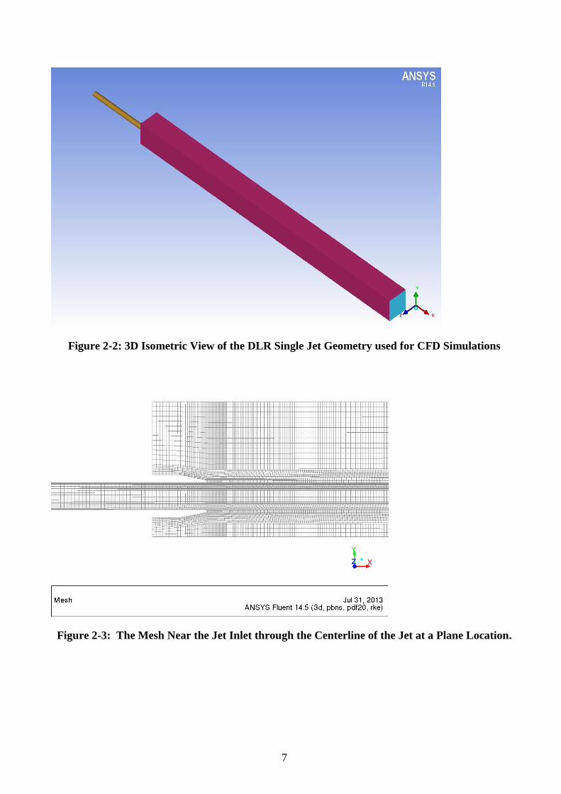
geometry where the combustor wall is assumed to be one boundary. Figure 2-2 shows a 3D isometric

view of the CFD geometry. The flow, see Figure 2-1, flows from bottom to top and dumps into the

ambient air at the exit plane of the combustor. The flow is in the positive x-direction for the CFD

model, see Figure 2-2. The mesh was created in ANSYS ICEM and consists of 543,672 hexahedral

cells. Figure 2-3 shows a portion of the mesh at a plane through the jet centerline.

Figure 2-1: 3D CAD Model and Photograph of the DLR Single Jet Experimental Rig [6]

7

Figure 2-2: 3D Isometric View of the DLR Single Jet Geometry used for CFD Simulations

Figure 2-3: The Mesh Near the Jet Inlet through the Centerline of the Jet at a Plane Location.

8

2.2 Scaled Siemens Combustion System

The Siemens combustion system was scaled with a geometrical linear scaling factor of 0.3 to fit into

the high pressure test rig at the DLR in Stuttgart. Also, the combustor basket was replaced with a

rectangular combustor with quartz wall to allow for optical measuring techniques. Figure 2-4 shows a

photograph of the entire high pressure test rig, Figure 2-5 shows a CAD model of the test rig, and

Figure 2-6 shows a cross sectional view of the burner. The geometry used for the CFD model

consisted of a 90 degree section with the combustor wall as one boundary. The 90 degree section and

periodic boundary conditions were used to reduce computational time. An isometric view of the CFD

geometry can be seen in Figure 2-7. Figure 2-8 shows a portion of the mesh at a cut plane through the

center of the burner. The mesh was provided by ANSYS, and consists of 8,063,111 polyhedral cells.

Figure 2-4: Photograph of the Experimental Test Rig [10].

Figure 2-5: CAD Model of the Experimental Test Rig [2].

9

Figure 2-6: Cross Section View of the Scaled Siemens Burner [2].

Figure 2-7: Isometric View of the Geometry used in the CFD Simulation

10

Figure 2-8: A Portion of the Mesh at a plane location z = 0 near the Pilot/Swirler Region.

11

3 ANALYSIS – DLR SINGLE JET

The DLR single jet study focused on comparing the FGM, BVM, and the FGM/BVM hybrid models

to experimental data for H2 and CH4 as the fuel composition. The experimental data available for

comparison consisted of PIV data and Raman temperature data. The data has been normalized using

the inlet jet diameter, the jet average velocity, and the adiabatic temperature.

3.1 Operating and Boundary Conditions

All operating and boundary conditions were selected to match the experimental conditions. The

operating pressure is 1 atm. The inlet of the jet is assumed to be perfectly premixed, and the air/fuel

ratio is in the lean regime and for hydrogen and methane an equivalence ratio of 0.72 was used.

Turbulence was introduced at the inlet boundary with the input parameters being the hydraulic

diameter and turbulent intensity, the turbulent intensity was approximated using a correlation in the

Fluent theory guide [3]. The boundary conditions were set to match the experiments

3.2 Results and Discussion

The CFD results are compared to PIV velocity flow field data and Raman scattering temperature data.

Figure 3-1 and Figure 3-2 shows contour plots of the normalized X velocity for H2 and CH4 as the

fuel for a.) BVM, b.) FGM, c.) FGM/BVM hybrid, and d.) PIV data, respectively. The turbulence

model for each case remained the same and a consistent under prediction of the velocity gradient was

observed in the x direction. The poor prediction of the velocity field can be attributed to three sources

of errors: 1.) the turbulence model was not optimized for each case and limitations with RANS

modeling, 2.) The heat loss at the wall was accounted for by assuming an imposed wall temperature

arbitrarily chosen, and 3.) Neglected radiation heat loss effects.

Figure 3-3 and Figure 3-4 shows contour plots of the normalized temperature for H2 and CH4 as the

fuel for a.) BVM, b.) FGM, c.) FGM/BVM hybrid, and d.) PIV data, respectively. The contour plots

in Figure 3-3 do not show any significant differences for the hydrogen case between each model

except for slight high temperature regions in the FGM model seem to be lifted. However, in Figure

3-4 both the FGM and the FGM/BVM hybrid model captures flame liftoff whereas the BVM model is

completely anchored. The flame location is highly dependent on the coupling between turbulence and

chemistry, and optimization of the turbulence model or higher accuracy models such as large eddy

simulations (LES) are needed to increase the accuracy.

12

a.)

b.)

c.)

d.)

Figure 3-1: Normalized X Velocity Comparison between a.) BVM b.) FGM c.) FGM/BVM

Hybrid and d.) PIV Data for the Hydrogen Case

13

a.)

b.)

c.)

d.)

Figure 3-2: Normalized X Velocity Comparison between a.) BVM b.) FGM c.) FGM/BVM

Hybrid and d.) PIV Data for the Methane Case

14

a.) b.)

c.) d.)

Figure 3-3: Normalized temperature Comparison between a.) BVM b.) FGM c.) FGM/BVM

Hybrid and d.) PIV Data for the Hydrogen Case

15

a.) b.)

c.) d.)

Figure 3-4: Normalized temperature Comparison between a.) BVM b.) FGM c.) FGM/BVM

Hybrid and d.) PIV Data for the Methane Case

16

A quantitative comparison of the axial normalized temperature profile along the centerline of the jet

for the hydrogen case is shown in Figure 3-5. The experimental data shows a larger negative

temperature gradient in the x direction after the reaction zone, which can be explained by heat loss due

to radiation. The inlet normalized temperature of the experimental data shows a contradiction with the

boundary conditions provided by difference of 0.04. The most likely cause is heat loss due to poor

insulation in the inlet pipe prior to entering the combustor or uncertainty in the measurements. The

CFD thermal boundary condition at the inlet was adjusted for the FGM case to demonstrate the effect

on the computational solution. Figure 3-6 shows a.) normalized X velocity and b.) normalized

temperature contour plots with an inlet normalized temperature of 0.22 for the FGM with hydrogen

case. An under prediction of the velocity gradient in the x direction is still observed with an inlet

normalized temperature of 0.22, see Figure 3-6a. The normalized temperature contour in Figure 3-6b

shows the physical phenomena of flame liftoff is captured with the FGM model with an inlet

normalized temperature of 0.22, and the significant deviation from experimental results are from an

inaccurate turbulence model. Figure 3-7 shows the axial normalized temperature comparison of the

FGM case with an inlet normalized temperature of 0.26 and 0.22 to the experimental data. Although

the axial profile along the centerline of the jet seems to deviate further away from experimental results

when the inlet temperature is reduced, the slope of the temperature profile in the reaction zone is better

predicted. The better prediction in the slope demonstrates that FGM captures chemical effects due to a

decrease in inlet temperature, i.e. slower reaction rates. Figure 3-8 shows the axial normalized

temperature profile along the centerline for the different models with methane as the fuel. Although

the CFD data differs significantly from the experimental data, the FGM and the FGM/BVM hybrid is

superior to the BVM model.

Figure 3-5: Axial Normalized Temperature Profile Comparison along the Centerline of the Jet

for the Hydrogen Case

17

a.)

b.)

Figure 3-6: a.) Normalized X Velocity and b.) Normalized Temperature Contours with an Inlet

Normalized Temperature of 0.22 for the FGM with Hydrogen Case

18

Figure 3-7: Axial Normalized Temperature Comparison of the FGM Case with Hydrogen at

Different Normalized Inlet Temperatures

Figure 3-8: Axial Normalized Temperature Profile Comparison along the Centerline of the Jet

for the Methane Case

19

4 ANALYSIS – SCALED SIEMENS COMBUSTION SYSTEM

The scaled Siemens combustion system case used the FGM combustion model with methane as the

fuel. Experimental data was available with a hydrogen/methane blend in the main fuel supply and

methane in the pilot. Unfortunately, a limitation of the mixture fraction formulation only allows for a

single composition of fuel with the same temperature to be introduced at the boundaries. The

temperature at the inlet of the main and the pilot is significantly different, however since only small

portion of the fuel is going through the pilot, the flamelet was tabulated using the temperature at the

inlet of the main fuel. Also, by the same argument, the flamelet was tabulated using a premixed

flamelet although the region near the pilot is a diffusion flame. Therefore experimental data with only

methane in the pilot and mains could be considered for validation. Convergence of the CFD results

could only be achieved with first order accuracy, and those results are presented. The experimental

data is compared with the CFD simulation using the FGM combustion model. The CFD results are

also compared with the BVM model conducted in a study performed by Schmidl [2]. The author

urges the reader to refer to a detailed study by Schmidl, which used ANSYS CFX and the BVM for

the scaled Siemens combustion system [2]. In the study by Schmidl, second order convergence with a

steady state solver was not achieved and an unsteady RANS solution was averaged to obtain a stable

solution. Also, the collaboration work with ANSYS.inc applied only a first order upwind scheme. A

procedure to converge a second order solution should be developed either using unsteady RANS

averaging or a LES.

4.1 Operating and Boundary Conditions

The operating pressure of the scaled Siemens combustion system test rig is 4 bar. All mass flow inlets

are multiplied by a factor of 0.25 since the geometry is only a quarter section with periodic boundary

conditons. The air flow split to the pilot was assumed 8 percent. The actual split is unknown;

however, Scmidl [2] determined that an 8 percent split is a reasonable value. The boundary conditions

were selected to match the conditions experienced during testing. All walls except the combustor wall

are assumed adiabatic and the combustor wall is assumed a temperature of 1100 K to account for heat

loss. The main fuel inlet temperature is used, and the pilot fuel had to be assumed the same value in

order to use the FGM combustion model. Assuming the pilot and main fuel temperature values to be

the same will cause significant error near the pilot region, however the region away from the pilot,

which accounts for the majority of the heat release, should not have a significant effect.

4.2 Results and Discussion

The scaled Siemens combustion system is a significant step towards validating the FGM combustion

model for use in gas turbine engines. Robust experimental data in actual gas turbine engines are

extremely difficult to measure. The scaled Siemens combustion system test campaign conducted at

the DLR in Stuttgart provided detailed velocity and temperature measurements inside the combustor.

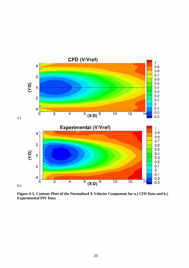
Figure 4-1 shows a contour plot of normalized X velocity component in the a.) FGM CFD results and

b.) PIV experimental results. The recirculation zone seems slightly stretched in the CFD results. Once

again, turbulence modeling seems to be a major limitation in the study. Qualitatively, the flame

location is compared in Figure 4-2, which shows contour plots of a.) OH mass fractions and b.)

OH*Chemiluminescense. The CFD results predict the flame location reasonably well, but there is

some reaction quenching near the walls of the combustor, due to an inadequate thermal boundary

condition at the combustor wall, poor turbulence modeling, and/or the neglect of radiation heat

transfer.

20

a.)

b.)

Figure 4-1: Contour Plots of the Normalized X Velocity Component for a.) CFD Data and b.)

Experimental PIV Data

21

a.)

b.)

Figure 4-2: Contour Plots of a.) CFD OH Mass Fractions and b.) Experimental OH*

Chemiluminescense

22

A quantitative comparison of the FGM combustion model, the BVM model, and experimental data is

presented next. Figure 4-3 compares different axial profiles (along the x direction) at different radial

locations (along the z direction) using the FGM model in ANSYS Fluent. Figure 4-4 is a similar

comparison using the BVM and different turbulence models, refer to Scmidl [2] for further

clarification. From Figure 4-3 and Figure 4-4, the BVM and the FGM model over predict the

temperature at a radial location of z = 0 mm and z = 20 mm. The BVM predicts the temperature at an

axial location of z = 34 mm much better than the FGM, but the FGM does a better job at z = 39 mm.

The analysis with the FGM model made no effort to optimize the turbulence model and the solution

was solved with first order accuracy using a steady state RANS k-epsilon realizable turbulence model.

The BVM analysis used multiple unsteady RANS turbulence models with higher order accuracy. The

error near the centerline for both studies can be attributed to inaccurate modeling of turbulence,

premixed flamelet assumption, and assuming the pilot fuel inlet temperature was the same as the main

fuel inlet temperature. Also, both analysis neglected radiation heat transfer, which is important in

combustion.

Figure 4-3: Axial Temperature Profiles at Different Radial Locations for the FGM Analysis and

Experimental Data

23

Figure 4-4: Axial Temperature Profiles at Different Radial Locations for the BVM Analysis and

Experimental Data [2].

24

5 CONCLUSION

Results from a CFD study using the FGM combustion model with the DLR single jet geometry was

presented and compared to the BVM and FGM/BVM hybrid combustion models. In most cases the

capability of FGM and/or FGM/BVM hybrid in predicting flame location and capture the phenomena

of flame liftoff is superior to the BVM. The effect different fuels had on flame structure and location

were clearly seen with the FGM and/or FGM/BVM hybrid combustion model, whereas the BVM

model showed lack of clarity. In some instances, the FGM/BVM hybrid model and the FGM model

are in agreement, see Figure 3-4 and Figure 3-8. In other instances, the FGM demonstrated better

prediction capabilities, see Figure 3-5. The turbulence model used in the present analysis is the

limiting factor, and an optimized RANS model or LES is needed to accurately predict combustion

parameters.

The scaled Siemens combustion system case provided great insight into the capabilities and limitations

of the FGM combustion model. The modeling limitations in using any combustion model based on

mixture fraction formulation is only one fuel composition and temperature at the inlets, unless multiple

mixture fractions are defined. Unfortunately, most gas turbine engines do not fit into this category.

Assumptions, such as assume the fuel temperature is the same as the main fuel inlet temperature and a

premixed flamelet for chemistry tabulation, can lead to reasonable results except in the pilot region.

The velocity contour plot from Figure 4-1a is in good agreement with the experimental PIV data in

Figure 4-1b. Near the walls of the combustor the FGM analysis predicted the temperature profile in

the axial direction better than the BVM analysis conducted by Schmidl. A stable solution could only

be achieved using first order upwind with a steady RANS model. A Similar problem was encountered

in the BVM analysis conducted by Scmidl [2], and an unsteady RANS approach was used to reach a

stable solution. A more in-depth study on the scaled Siemens combustion case is needed to determine

if FGM is superior to the BVM combustion model.

The FGM and the FGM/BVM hybrid model show promising results for turbulent combustion

modeling. Caution needs to be made when determining which flamelet to use, i.e. premixed/non-

premixed and fuel/oxidizer temperatures. The model was successfully performed in ANSYS Fluent,

including flamelet generation. Flamelets built using Fluent should be checked and verified that a

physical solution is given. Fluent has the ability to import custom flamelet tables with more

controlling variables such as scalar dissipation, heat loss, etc. Custom flamelet table generation gives

the user the ability to achieve more accurate solutions.

Further development and validation of the FGM and FGM/BVM hybrid model is recommended before

use in product development. The DLR single jet and scaled Siemens combustion system have a wide

range of experimental data to validate the models, but significant effort in modeling turbulence with

greater accuracy is recommended. An in depth sensitivity analysis on the maximum scalar dissipation

at stoichiometric mixture fraction is recommended to determine the ability to tune the combustion

model. The development of a procedure to calculate a value for the maximum scalar dissipation at

stoichiometric mixture fraction based on knowledge of the flow field and the use of a chemical solver

such as CANTERA would provide an approximate value based on physics. A completely physics

based option would involve custom built flamelet tables with scalar dissipation, mixture fraction, and

reaction progress as the controlling variables, and should be considered for future application.

25

AKNOWLEDGMENTS

I would like to express my sincere gratitude to Siemens Energy’s stationary components combustion

aero/thermal group for a rewarding internship experience. I would also like to acknowledge my

mentors Rich Valdes and Ray Laster for always making themselves available, and expanding my

engineering knowledge of gas turbine engines. Finally I would like to thank Southwest Research

Institute and the UTSR program for their support, without it this experience would not have been

possible.

26

REFERENCES

1. Oijen, J.A. Van, “Flamelet-Generated Manifolds: Development and Application to Premixed

Laminar Flames”, Eindhoven: Technische Universiteit Eindhoven, 2002.

2. Schmidl, B., “Validation of Advanced CFD-Combustion Models for Modern Lean Premixed

Burners”, Mülheim an der Ruhr, September 2011.

3. ANSYS, Inc. “ANSYS FLUENT Theory Guide”, Release 14.5, 2012

4. Goldin, G.; Ren, Z.; Hendrik, F.; Lu, L; Tangirala, V.; and Karim, H. ”Modeling CO with

Flamelet-Generated Manifolds. Part 1: Flamelet Configuration”, Proceedings from the Turbo

Expo, Copenhagen, Denmark. 2012.

5. Goldin, G.; Ren, Z.; Hendrik, F.; Lu, L; Tangirala, V.; and Karim, H. ”Modeling CO with

Flamelet-Generated Manifolds. Part 2 - Application”, Proceeding from the Turbo Expo,

Copenhagen, Denmark. 2012.

6. DLR, “ Hochtemperaturverbrennung Messkampagne Eingeschlossene Jetflamme”, Internal

Reprot, Stuttgart, Germany, 2008.

7. DLR, “Messkampagne Eingeschlossene Jetflamme Zusatzliche Wasserstoffflammen – H2 PIV

90 m/s“, Internal Report, Stuttgart, Germany.

8. DLR, “Messkampagne Eingeschlossene Jetflamme Zusatzliche Wasserstoffflammen – H2

Raman 90 m/s“, Internal Report, Stuttgat, Germany.

9. DLR COORTEC-turbo 2.1.3, “Flame Stabilization Mechanisms for Robust Burner System with

Increased Fuel Flexibility“, Internal Report,Stuttgart, Germany, 2010.