T:issuesW3GCAJE49 3R18caje 12218 - University of Oxfordusers.ox.ac.uk/.../zanetti_theodorodes_CJE2017_caje12218.pdf · News shocks and labour market dynamics 907 1. Introduction A

Canadian Journal of Economics / Revue canadienne d’economique, Vol. 49, No. 3August 2016. Printed in Canada / Aout 2016. Imprime au Canada

0008–4085 / 16 / 906–930 / © Canadian Economics Association

News shocks and labour market dynamics inmatching models

Konstantinos Theodoridis Bank of EnglandFrancesco Zanetti University of Oxford

Abstract.We enrich a baseline real business cycle (RBC) model with search and matchingfrictions on the labour market and real frictions that are helpful in accounting for theresponse of macroeconomic aggregates to shocks. The analysis allows shocks to have anunanticipated and a news (i.e., anticipated) component. The Bayesian estimation of themodel reveals that the model that includes news shocks on macroeconomic aggregatesproduces a remarkable fit of the data. News shocks in stationary and non-stationary TFP,investment-specific productivity and preference shocks significantly affect labour marketvariables and explain a sizeable fraction of macroeconomic fluctuations at medium- andlong-run horizons. Historically, news shocks have played a relevant role for output, butthey have had a limited influence on unemployment.

Resume. Nouvelles et dynamique du marche du travail dans les donnees et dans les modelesd’arrimage. Les auteurs enrichissent un modele de cycle d’affaires reel (CAR) d’un lissagede la consommation, d’une prise en compte de l’utilisation du capital, du cout d’ajustementde l’investissement, et des frictions dans l’arrimage sur le marche du travail, en plusd’introduire des chocs de nouvelles dans la macroeconomie et le marche du travail. Lemodele est calibre en utilisant des donnees sur la macroeconomie et sur le marche dutravail, et son habilete a s’ajuster aux series economiques est remarquable. D’une manierequi cadre bien avec les resultats de la litterature sur le CAR, la calibration identifie l’effetnon-lineaire du choc positif dans la productivite attribuable au travail en tant que sourcemajeure du dynamisme economique, alors que la nouvelle a propos de ce choc joue un rolemineur. C’est le cas pour la plupart des chocs anticipes dans ce modele, a cette exceptionpres que la nouvelle d’un choc dans la productivite attribuable a la fonction d’arrimagelaquelle a un pouvoir substantiel d’explication du chomage et de la probabilite de trouverun emploi. Finalement un choc non anticipe dans la destruction d’emplois explique uneportion importante du chomage aux Etats-Unis.

JEL classification: E32, C32, C52

We would like to thank Paul Beaudry, Wouter den Haan, Charlotte Dendy, Monique Ebell,Alexandre Janiak, Francisco Ruge-Murcia, Lydia Silver, Yaniv Yedid-Levi and seminarparticipants at the Bank of England, London School of Economics, University of Oxford andthe Annual Congress of the European Economic Association in Toulouse for extremely valuablecomments. Francesco Zanetti acknowledges financial support from the Leverhulme TrustResearch Project Grant. This paper represents the views and analysis of the authors and shouldnot be thought to represent those of the Bank of England.Corresponding author: Francesco Zanetti, [email protected]

News shocks and labour market dynamics 907

1. Introduction

A number of studies establish that anticipated changes in future technology,referred to as news shocks, represent an important source of business cyclefluctuations.1 Extensive research has focused on the effect of news on economicactivity, but no studies have so far investigated its effect on labour market vari-ables. This paper fills this gap. We enrich a baseline real business cycle (RBC)model with search and matching frictions on the labour market and real fric-tions (consumption smoothing, capital utilization, investment adjustment cost),which are helpful in accounting for the response of macroeconomic aggregatesto shocks. The exogenous driving forces of the model are unanticipated and news(i.e., anticipated) shocks to permanent and stationary total factor productivity(TFP), investment-specific productivity, preference, matching technology and jobdestruction. Using this framework, we investigate to what extent are distinct newsshocks important to explain fluctuations in labour market variables and macro-economic aggregates, and we study the propagation dynamics of relevant newsshocks.

To confront the theoretical framework with the data, the model allows, butdoes not require, news shocks to interact with unanticipated shocks to generateaggregate fluctuations. It therefore allows both sources of exogenous disturbancesto simultaneously compete to explain the data. The Bayesian estimation of themodel reveals that the data prefer a version of the model that includes news shocksto stationary and non-stationary TFP, investment-specific productivity and pref-erence shocks. Specification with labour market news only (anticipated shocksto matching technology and the job destruction rate), with all sources of newsshocks or without any source of news shocks are unsupported by the data. Theanalysis shows that despite the presence of labour market news shocks substan-tially increases the performance of the model relative to the version without newsshocks. However, it diminishes the model forecast fit of output, consumption andinvestment when macroeconomic news shocks are present, thereby worsening theoverall fit of the model.

The analysis shows that the model with macroeconomic news shocks matchesthe data remarkably well. In addition, unanticipated shocks to stationary TFP ex-plain the bulk of fluctuations in output, wages, vacancies and labourmarket tightness in the one quarter ahead. Subsequently, for the one-year-, three-year- and 10-year-ahead horizons, news shocks to the stationary TFP become animportant source of fluctuations in aggregate variables, similar to findings inSchmitt-Grohe and Uribe (2012). Historical variance decomposition shows thatnews shocks are a relevant source of fluctuation for consumption and output inthe US postwar data whereas they play a limited role for unemployment. Finally,the model is able to identify the effect of news disturbances on labour marketand macroeconomic variables. We find that the responses of macroeconomicaggregates in the anticipation phase of the news shock differ from the responses1 See Beaudry and Portier (2014) and references therein for a recent review on the literature.

908 K. Theodoridis and F. Zanetti

in the aftermath of the realization of the shock. For instance, in the anticipationof the news shock to the stationary TPF, the marginal product of labour risessince the expected higher productivity induces the firm to reduce labour input.Consequently, as wages increase, the firm decreases its vacancy postings, leadingto a rise in unemployment that induces a fall in labour market tightness and thejob-finding rate. However, once the shock realizes, employment sharply increases,reducing the marginal product of labour and, consequently, wages, whose effectis to reverse the variables’ responses in the anticipation phase and mimic the stan-dard dynamics of the unanticipated TFP shock. Similarly, the analysis shows thatdifferent dynamics during the anticipation and the realization periods are presentin the other shocks.

Before proceeding with the analysis, we describe the relationship of the pa-per with related studies. The view that expectations generate economic fluctua-tions has been recently revisited in a series of influential papers by Beaudry andPortier (2004, 2006) and Barsky and Sims (2011), who develop VAR method-ologies to identify the effect of news shocks on economic activity. In addition,Kurmann and Otrok (2013) also use a similar VAR methodology to show thatnews shocks provide strong linkages between the yield curve, inflation and realoutput. This analysis is complemented by recent studies by Beaudry and Portier(2006), Schmitt-Grohe and Uribe (2012), Khan and Tsoukalas (2012) and Gortzand Tsoukalas (2011), who identify and estimate news shocks in the context offully specified general equilibrium models. Our paper contributes to both realmsof research by identifying the effect of news shocks on labour market aggregatesin the context of a fully specified general equilibrium model, with labour marketsearch and matching frictions estimated with Bayesian methods. In contrast tothe existing studies, we extend the analysis to identify the effect of news shocks onlabour market aggregates, allowing for news shocks in labour market variables.

This paper also contributes to research that investigates to what extent newsshocks improve the performance of theoretical models in matching businesscycle fluctuations. Influential studies by Jaimovich and Rebelo (2009), Den Haanand Kaltenbrunner (2009) and Karnizova (2010) show that news shocks improvethe empirical performance of theoretical models. However, they also indicate thatstandard real business cycle models are unable to generate positive co-movementsof macroeconomic aggregates in response to news shocks, and they propose dif-ferent modifications to address this shortcoming. Similarly to our paper, DenHaan and Kaltenbrunner (2009) find that labour market frictions enhance theperformance of the model in matching the reactions of consumption, outputand investment in response to news shocks. Our analysis differs substantially intwo ways. First, it is the first study that focuses on the effect of news shocks onlabour market variables, namely wages, unemployment and the job-finding rate.Second, our theoretical findings are more general because we use a baseline searchand matching model, whereas these authors develop a model with endogenouslabour force participation. Our analysis shows that a relatively standard modelwith labour market search and matching frictions is able to replicate fluctuations


in macroeconomic aggregates fairly well. In this respect, our results are relatedto and reinforce the findings in Leeper and Walker (2011) and Barsky and Sims(2011), which suggest that real business cycle models are able to replicate theresponses of macroeconomic aggregates to news shocks, without any need todepart from the standard framework.

The remainder of the paper proceeds as follows. Section 2 lays out the modeland presents the econometric methodology and data. Section 3 presents theestimation results, comprising the empirical fit and forecasting performance ofalternative models, the effect of news shocks on labour market variables and theirrelevance to explain historical fluctuations. Finally, section 4 concludes.

2. The model

We now set up a simple general equilibrium model with labour market searchand matching frictions. We introduce a matching process for hiring in the labourmarket, as in the Mortensen–Pissarides model and similar to Den Haan andKaltenbrunner (2009) and Thomas (2011), and we enrich the model withanticipated news shocks, as in Schmitt-Grohe and Uribe (2012) and Khan andTsoukalas (2012).

Three agents populate the model economy: households, firms and a passivefiscal authority. Households consist of a large number of members, a fraction ofwhich are unemployed and searching for jobs. On the other side of the labourmarket, firms hire workers by posting vacancies. The fiscal authority balances thebudget in every period with lump-sum transfers. The rest of this section describesthe agents’ tastes, technologies and the structure of the labour market in detail.

2.1. FirmsEmployment relationships are taken to consist of two agents, a worker and a firm,which engage in production through discrete time until the relationship is severed.Firms post a number of vacancies. Unemployed workers and vacancies, whichare denoted by ut and vt, respectively, meet in the so-called matching function,m(vt, ut). Normalizing the size of the labour force to 1, ut also represents the unem-ployment rate and ut ≡1−nt−1. Under the assumption of constant returns to scalein the matching function, the matching probabilities for unemployed workers:

m(vt, ut)ut

=m(

vt

ut, 1

)≡p(xt),

and for vacancies,

m(vt, ut)vt

=m(

1,1

vt=ut

)≡q(xt),

are functions of the ratio of vacancies to unemployment, xt ≡ vt=ut, also calledlabour market tightness. Notice that p′(xt) > 0 and q′(xt) < 0, i.e., in a tighter


labour market, jobseekers are more likely to find jobs and firms are less likely tofill their vacancies. Notice also that p(xt)=xtq(xt).

The law of motion of the firm’s workforce, nt, is therefore given by:

nt =(1− ±n,t

)nt−1 +q(xt)vt, (1)

where q(xt)vt is the number of new matches at time t and ±n,t is the job destructionrate that follows the autoregressive process:

ln ±n,t =(1−½±n

)ln ±n +½±n ln ±n,t−1 +¾±n"±n,t +¾t+4,±nÃ±n,t=t+4

+¾t+8,±nÃ±n,t=t+8,(2)

with 0 < ½±n < 1 and where the zero-mean, serially uncorrelated innovations "±n,t,Ã±n,t=t+4 and Ã±n,t=t+8 are normally distributed with standard deviation ¾±n ,¾t+4,±n and ¾t+8,±n . In this notation, "±,t represents the unanticipated shock tothe job destruction rate, whereas Ã±n,t=t+4 and Ã±n,t=t+8 represent the anticipatedt +4 and t +8 periods ahead news shocks to the job destruction rate, respectively,that bear no contemporaneous effect on the level of the job destruction rate. Asshown in Theodoridis and Zanetti (2014) and Zanetti (2015), adding exogenousshocks to the job destruction rate improves the ability of a very stylized businesscycle model to replicate the unemployment dynamics and other important labourmarket statistics.

The firm’s production function is given by:

yt =atkμt(°tnt

)1−μ, (3)

where kt and nt denote capital and labour services, respectively, and at and °t arethe stationary and non-stationary total factor of productivity (TFP) shocks. Thestationary TFP shock, at, follows the autoregressive process:

ln at =½a ln at−1 +¾a"a,t +¾t+4,aÃa,t=t+4 +¾t+8,aÃa,t=t+8, (4)

with 0 < ½a < 1 and where the zero-mean, serially uncorrelated innovations "a,t,Ãa,t=t+4 and Ãa,t=t+8 are normally distributed with standard deviations ¾a, ¾t+4,aand ¾t+8,a, respectively. In this notation, "a,t represents the unanticipated shockto TFP, whereas Ãa,t=t+4 and Ãa,t=t+8 represent the anticipated t + 4 and t + 8periods ahead news shocks to TFP, respectively. The growth rate of the non-stationary, labour augmented TFP shock, zt, is stationary and follows the au-toregressive process:

ln zt = ln(

°t

°t−1

)= (

1−½z)

ln z +½z ln zt−1 +¾z"z,t

+¾t+4,zÃz,t=t+4 +¾t+8,zÃz,t=t+8,(5)

with 0 < ½z < 1, and where the zero-mean, serially uncorrelated innovations "z,t,Ãz,t=t+4 and Ãz,t=t+8 are normally distributed with standard deviations ¾z, ¾t+4,z


and ¾t+8,z, respectively. In this notation, "z,t represents the unanticipated shockto the growth rate of the non-stationary labour augmented TFP shock, whereasÃz,t=t+4 and Ãz,t=t+8 represent the anticipated t +4 and t +8 periods ahead newsshocks, respectively. Finally, capital services, kt, depends on the utilization rate,Àt:

kt =Àtkt−1, (6)

where kt−1 is the installed physical capital in period t −1.

2.1.1 Profit maximizationSubject to equations (1) and (3), the firm maximizes its profits:

E0

∞∑t=0

¯t¸t

[yt −ntwt −ktqk

t − vtgt

], (7)

where ¯t¸t measures the marginal utility value to the representative householdof an additional dollar in profits received during period t, wt is the real wage paidto the worker, qk

t is the remuneration rate for each unit of capital kt and gt isthe real cost of hiring (defined below), which is taken as given by the firm. As inGertler and Trigari (2009) and Mandelman and Zanetti (2014), the cost of hiringis a function of labour market tightness xt, such that gt = B°tx®

t , where ® is theelasticity of labour market tightness with respect to hiring costs such that ®� 0and B �0 is a scale parameter.

Thus the firm chooses {kt, nt, vt}∞t=0 to maximize equation (7), subject to equa-

tions (1) and (3). By substituting equation (3) into equation (7) and letting »tdenote the non-negative Lagrange multiplier on equation (1), the first-order con-ditions are:

qkt = μyt=kt, (8)

wt = (1− μ)yt=nt − »t +(1− ±n,t

)¯Et(¸t+1=¸t)»t+1 (9)

and:

gt =q(xt)»t. (10)

Equation (8) assumes that the rate of capital remuneration, qkt , equals the

marginal product of capital in each period t, μyt=kt. Equation (9) equates the realwage, wt, to the marginal rate of transformation. The marginal rate of transfor-mation depends on the marginal product of labour, (1− μ)yt=nt, but also, due tothe presence of labour market frictions, on present and future foregone costs ofhiring. The latter two components are the shadow value of hiring an additionalworker, »t, net of the savings in hiring costs resulting from the reduced hiringneeds in period t+1 if the job survives job destruction, (1−±n,t)¯Et(¸t+1=¸t)»t+1.In a model without labour market search, only the marginal product of labour


appears. Finally, equation (10) states that the cost of posting an additionalvacancy, gt, equals the expected benefits that the additional hiring takes intoproduction, q(xt)»t.

2.2. HouseholdsThere exists a representative household. A fraction (nt) of its members are em-ployed and the remaining members are unemployed and searching for jobs. Allmembers pool their resources to ensure equal consumption (ct). The householdutility function is:

E0

∞∑t=0

¯t

⎡⎢⎣dt

(ct°t

−h ct−1°t−1

)1−¾

1−¾−Â

n1+Át

1+Á

⎤⎥⎦, (11)

where dt is a consumption preference shock that follows the autoregressive pro-cess:

ln dt =½d ln dt−1 +¾d "d ,t +¾t+4,d Ãd ,t=t+4 +¾t+8,d Ãd ,t=t+8, (12)

with 0 < ½d < 1 and where the zero-mean, serially uncorrelated innovations "d ,t,Ãd ,t=t+4 and Ãd ,t=t+8 are normally distributed with standard deviations ¾d , ¾t+4,dand ¾t+8,d , respectively. The parameter 0 < h < 1 describes the degree of habit inconsumption, ¾ > 0 is the intertemporal rate of substitution, Á > 0 is the inverseof the Frisch elasticity of labour supply and Â > 0 is the degree of disutility ofworking. The household budget constraint is:

wtnt +[qk

t Àt −#(Àt

)]kt−1 + ft + ¿t = ct + it, (13)

where wtnt is the remuneration of labour, qkt Àtkt−1 is the remuneration from

renting Àtkt−1 units of capital services at the rate qkt , the term #(Àt)kt−1 describes

the cost of capital utilization,2 ft are real profits reverted from the firm sectorto households in lump-sum transfers, ¿t are real lump-sum transfers from thegovernment and it are the units of output invested. By investing it units of outputduring period t, the household increases the installed capital stock kt accordingto:

kt = (1− ±k)kt−1 +$t

[1−S

(it

it−1

)]it, (14)

where the depreciation rate satisfies 0 < ±k < 1 and S(·) is an adjustment costfunction that satisfies S(z) = 1, S′(z) = 1 and S′′(·) > 0. The investment-specificshock, $t, follows the autoregressive process:

ln $t =½i ln $t−1 +¾i"i,t +¾t+4,iÃi,t=t+4 +¾t+8,iÃi,t=t+8, (15)

2 The function #(Àt) satisfies the conditions: #(1)=0, #′(·) > 0 and #′′(·) > 0.


with 0 < ½i < 1 and where the zero-mean, serially uncorrelated innovations "i,t,Ãi,t=t+4 and Ãi,t=t+8 are normally distributed with standard deviations ¾i , ¾t+4,iand ¾t+8,i , respectively.

Thus the household chooses{ct, Àt, it, kt}∞t=0 to maximize its utility (11) subject

to the budget constraint (13) and the evolution of capital stock (14) for all t =0, 1, 2,…. Letting ¸t and &t denote the non-negative Lagrange multipliers withrespect to the household’s budget constraint and physical capital accumulationequation, the first-order conditions are:

¸t°t =dt

(ct

°t−h

ct−1

°t−1

)−¾

−h¯dt+1

(ct+1

°t+1−h

ct

°t

)−¾

, (16)

qkt =#′(Àt), (17)

1=8t$t

(1−S

(it

it−1

)−S′

(it

it−1

)it

it−1

)

+¯Et8t+1¹t+1¸t+1

¸tS′

(it+1

it

)(it+1

it

)2 (18)

and:

8t =¯Et

{¸t+1

¸t

[(1− ±k

)8t+1 +qk

t+1Àt+1 −#(Àt+1

)]}, (19)

where 8t =&t=¸t is the Tobin’s Q. According to equation (16), the Lagrange multi-plier equals the household’s marginal utility of consumption, which accounts forpast consumption due to habits in consumption. Equation (17) equates the remu-neration of capital with the marginal cost of capital utilization. Finally, equations(18) and (19) describe the evolution of investment and Tobin’s Q, respectively.

2.3. The labour market and wage bargainingThe structure of the model guarantees that a realized job match yields somepure economic surplus. The split of this surplus between the worker and the firmis determined by the wage level, which is set according to the Nash bargainingsolution. That is, the firm and worker each receive a constant fraction of the jointmatch surplus, which is the sum of firm and worker surplus. The worker surplus,Sh

t , is given by the wage, wt, minus the worker’s opportunity cost of holding ajob, wt, plus the expected surplus in the next period t + 1 if the match survivesseparation, which yields:

Sht =wt −wt + (1− ±n,t)¯Et

¸t+1

¸tSh

t+1, (20)


where wt = (ÂnÁt )=¸t (i.e., the worker’s opportunity cost of holding a job comprises

the labour disutility). The Lagrange multiplier »t represents the firm surplus ofan additional worker (i.e., Sf

t ≡ »t). Hence, if we solve equation (9) with respectto »t, the firm surplus, Sf

t , is given by the marginal product of labour minus thewage and plus the expected surplus in the next period t +1 if the match survivesseparation, which yields:

Sft = (1− μ)yt=nt −wt + (1− ±n,t)¯Et

¸t+1

¸tSf

t+1. (21)

The total surplus from a match is the sum of the worker’s and firm’s surpluses,Sh

t +Sft . Let ´ denote the household’s bargaining power. Nash bargaining implies

that the household receives a fraction ´ of the total match surplus:

Sht =´(Sh

t +Sft ). (22)

Combining equations (20) to (22) and using the first-order condition for va-cancies, equation (10), to derive S f

t+1 = gt+1=q(xt+1), we can write the agreedwage as:

wt =´[(1− μ)yt=nt +¯Et

(¸t+1=¸t

)gt+1

]+ (1−´)(ÂnÁt )=¸t. (23)

Equation (23) shows that the wage comprises two components: first, for afraction ´, the marginal product of labour plus a reward from saving in hiringcosts in period t + 1; second, for a fraction 1 −´, the worker’s opportunity costof holding a job.

2.4. Model solutionTo produce a quantitative assessment of the model, we need to parameterizethe matching function. Following Petrongolo and Pissarides (2001), we use thestandard Cobb–Douglas function:

mt =¹tu¹t v1−¹

t , (24)

where ¹ is the elasticity of the matching function with respect to unemploymentand ¹t is a shock to the efficiency of matching that follows the autoregressiveprocess:

ln ¹t=(1−½¹

)ln ¹+½¹ ln ¹t−1 +¾¹"¹,t +¾t+4,¹Ã¹,t=t+4 +¾t+8,¹Ã¹,t=t+8, (25)

with 0 < ½¹ < 1 and where the zero-mean, serially uncorrelated innovations "¹,t,Ã¹,t=t+4 and Ã¹,t=t+8 are normally distributed with standard deviations ¾¹, ¾t+4,¹and ¾t+8,¹, respectively. Combining the firm’s profit conditions (7), the house-hold’s budget constraint (13) and the assumption that the government balancesthe budget with lump-sum transfers produces the aggregate resource constraint:

yt = ct + it + vtgt +#(Àt)kt−1. (26)

The equilibrium conditions do not have an analytical solution. Consequently,the system is approximated by loglinearizing its equations around the station-ary steady state. In this way, a linear dynamic system describes the path of the


endogenous variables’ relative deviations from their steady-state value, account-ing for exogenous shocks.3 The solution to this system is derived using Klein(2000).

3. Econometric methodology, data and prior distribution

We estimate the model using Bayesian methods. To describe the estimation pro-cedure, define 2 as the parameter space of the DSGE model and ZT ={zt}T

t=1 asthe data observed. According to Bayes’ theorem, the posterior distribution of theparameter is of the form P(2|ZT ) ∝ P(ZT |2)P(2). This method updates the apriori distribution using the likelihood contained in the data to obtain the condi-tional posterior distribution of the structural parameters. To approximate the pos-terior distribution, we employ the random walk Metropolis–Hastings algorithm.The sequence of retained draws is stable, providing evidence on convergence.4 Theposterior density P(2|ZT) is used to draw statistical inference on the parameterspace 2. An and Schorfheide (2007) and Ruge-Murcia (2007) provide a detaileddescription of Bayesian simulation techniques applied to the DSGE models.

The econometric estimation uses US quarterly data for the period 1960:1–2007:4. We use data for output growth, consumption growth, investment growth,the unemployment rate and the job-finding rate. The macroeconomic series arean updated version of Smets and Wouters (2007),5 the unemployment rate is fromFRED and the job-finding rate is from Shimer (2012).

Our empirical strategy consists in estimating the 34 parameters in the modelthat are related to the preferences, technologies and exogenous unanticipated andnews disturbances {Á, ´, Ák , h, ¹, μ, #, q, n, vg=y, ½z, ½a, ½i , ½d , ½¹, ½±n , ¾z, ¾a,¾i , ¾d , ¾¹, ¾±n , ¾t+4,z, ¾t+4,a, ¾t+4,i , ¾t+4,d , ¾t+4,¹, ¾t+4,±n , ¾t+8,z, ¾t+8,a, ¾t+8,i ,¾t+8,d , ¾t+8,¹, ¾t+8,±n}. We calibrate the remaining 9 parameters {¯, ±n, ±k , ¾, Â,B, ®, a, d , z, ¹}, whose values fulfill specific economic conditions or determinethe steady state of the model. We first describe the calibrated parameters. Thequarterly discount factor ¯ is estimated equal to 0.99, which pins down a realinterest rate equal to approximately 4%, a value commonly used in the literature.Consistent with US data, as in Gertler et al. (2008) and Mumtaz and Zanetti(2012), the value of the exogenous job separation rate, ±n, is set equal to 10.5%,and the value of the capital destruction rate, ±k , is set equal to 2.5%, as in Smetsand Wouters (2007). The intertemporal rate of substitution, ¾, is set equal to1 to nest log-utility. We allow the parameter of the disutility of labour, Â, totake the value that enables the model to match the estimated steady-state levelof employment equal to 0.70, the average employment rate during the post-war3 An appendix that details the steady-state and linearized model is available upon request from

the authors.4 For each chain, we collect 1,000,000 draws where the first 900,000 are discarded and from the

remaining 100,000 we save one of every 100 draws. We have access to a Matlab cluster with 32workers and we, therefore, run 32 chains. An appendix that details evidence on convergence isavailable upon request from the authors.

5 The data are downloadable from aeaweb.org/atypon.php?doi=10.1257/aer.97.3.586.


period. Similarly, we allow the scale parameter B to take the value that enables themodel to match the estimated share of hiring costs over total output, vg=y, equalto 2%.6 To satisfy the Hosios condition, which ensures that the equilibrium of thedecentralized economy is Pareto efficient, we impose that the elasticity of labourmarket tightness with respect to hiring costs, ®, is equal to the relative bargainingpower of the worker, ´=(1−´), that is ´=(1−´)=®.7 Finally, we assume that thesteady state values of the shocks {a,d ,z,¹} are conveniently normalized to one.

Table 2 reports the prior distributional forms, means and standard deviationsfor the estimated parameters. The priors on these parameters are in line with exis-tent studies and harmonized across different shocks. Naturally, each constrainedmodel uses a subset of these priors. We choose priors for these parameters basedon several considerations. The inverse of the Frisch intertemporal elasticity ofsubstitution in labour supply, Á, is normally distributed with a prior mean equalto 2, which is in line with micro- and macro-evidence, as detailed in Card (1994)and King and Rebelo (1999), with a standard error equal to 0.25. The wage bar-gaining parameter, ´, is assumed to be beta distributed with prior mean equal to0.5, as standard in the search and matching literature and with a standard errorequal to 0.1. The prior for the parameter controlling the investment adjustmentcosts, Ák , is normally distributed with a prior mean equal to 5 and a standarderror of 0.25. The habit parameter, h, is assumed to be beta distributed with a priormean equal to 0.75 and a standard error equal to 0.05, as in Smets and Wouters(2007). The elasticity of the matching function, ¹, is normally distributed with aprior mean equal to 0.5, as in Petrongolo and Pissarides (2001), and a standarderror equal to 0.06. The production capital share, μ, is normally distributed witha prior mean equal to 0.3, a value commonly used in the literature and a stan-dard error of 0.1. The steady-state share of hiring costs over total output, vg=y, isassumed to be normally distributed with a prior mean equal to 0.02, consistentwith Gali (2010), and a standard error equal to 0.2. The steady-state vacancyfilling probability, q, is assumed to be beta distributed with a prior mean of 0.9,as in Andolfatto (1996), and a standard error equal to 0.05. The steady-stateemployment rate, n, is assumed to be beta distributed with a prior mean of 0.7as in the data and a standard error equal to 0.05.

Let us now turn to the prior distributions of the shock parameters. The priorson the autoregressive components and standard errors of the stochastic processesare harmonized across different shocks. We assume that the persistence param-eters ½z, ½a, ½i , ½d , ½¹ and ½±n are beta distributed, with a prior mean equalto 0.75 and a prior standard deviation equal to 0.1. The standard errors of theunanticipated innovations ¾z, ¾a, ¾i , ¾d , ¾¹ and ¾±n follow an inverse-gammadistribution with a prior mean of 0.5 and a prior standard deviation of 0.2, whichis similar to Gertler et al. (2008). The standard errors of the anticipated innova-

6 By treating Â and B as residuals, we are able to derive closed-form solutions for the steady stateof the model.

7 Hosios (1990) and Thomas (2011) provide a formal derivation and further analysis on thiscondition.


tions four- and eight-quarter ahead ¾t+4,z, ¾t+4,a, ¾t+4,i , ¾t+4,d , ¾t+4,¹, ¾t+4,±n ,¾t+8,z, ¾t+8,a, ¾t+8,i , ¾t+8,d , ¾t+8,¹ and ¾t+8, ±n follow an inverse-gamma distribu-tion with a prior mean of 0.35 and a prior standard deviation of 0.2. To assignequivalent explanation power to unanticipated and news shocks, we have chosenthe prior mean distributions of the shocks such that the total variance of theunanticipated component is half of the total variance of the shock.

4. Results

In this section, we present the findings and analyze the model’s prediction. Toestablish the relevance of distinct news shocks, we estimate several versions of themodel and assess their empirical fit using the marginal likelihood of the estimatedmodel. Next, we evaluate models’ forecasting performance, using both the meansquare forecasting error (univariate) and the log-predictive density score (mul-tivariate) metrics. Finally, we investigate the dynamics properties of the modelby using impulse response functions, forecasting variance decompositions andhistorical variance decomposition.

4.1. Model estimation fit and forecasting performanceThe model allows, but does not require, distinct news shocks to interact withunanticipated shocks to generate aggregate fluctuation. To evaluate the impor-tance of the different news shocks, we estimate four different versions of themodel that embed alternative combinations of news shocks:

• A version of the model without news shocks• A version of the model with labour market news shocks only (i.e., antici-

pated shocks to the job destruction rate and matching function)• A version of the model with macroeconomic news shocks only (i.e., an-

ticipated shocks to stationary TFP, to non-stationary labour augmentedshocks, to consumption preference and to investment-specific shocks)

• A version of the model with both macro and labour market news shocks

Before looking into the parameters’ estimates, we assess the overall perfor-mance of competing versions of the model. To establish which theoretical frame-work better replicates the data, we use the log-marginal likelihood. Thelog-marginal likelihood represents the posterior distribution, with the uncertaintyassociated with parameters integrated out, and therefore it also outlines the em-pirical performance of the model. The log-marginal likelihood is approximatedusing the modified harmonic mean, as detailed in Geweke (1999). As shown inthe fourth row of table 1, the log-marginal likelihood associated with the modelthat allows only for macroeconomic news is the highest among the constrainedalternatives and equal to −713.06, followed by the model that includes all sourcesof news shocks that has a log-marginal likelihood equal −797.06. Instead, theversions of the model without any source of news shocks or with labour marketnews deliver only a worse fit of the data.


TABLE 1Log-marginal likelihood, model comparison

Model Value

(1) No news −879.93(2) Labour market news −930.58(3) Macroeconomic news −713.06(4) Macroeconomic and labour market news −797.10

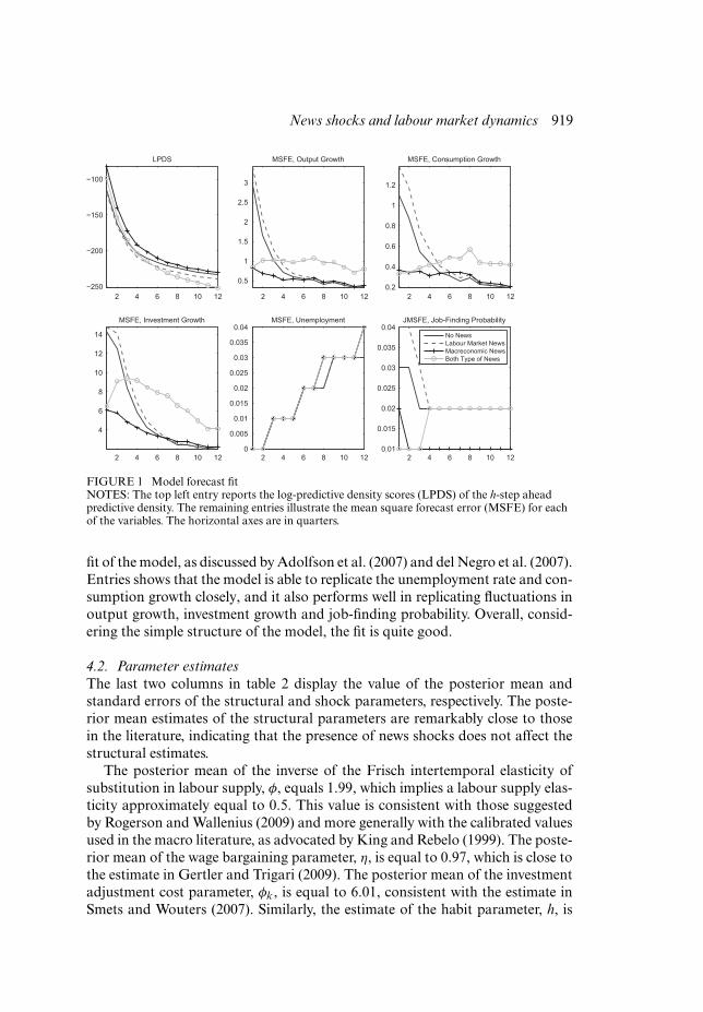
To investigate why the model with macroeconomic news outperforms the al-ternative models, we use the log-predictive density score (LPDS) and the meansquare forecast error (MSFE) for each of the observed variables.8 We use thesemetrics based on documentation by Adolfson et al. (2007) of close connectionbetween the log-marginal likelihood and the LPDS of the h-step-ahead predictivedensity. Furthermore, under the normality assumption on the functional form ofthe predictive density, there is a direct mapping between LPDS and MSFE thatmakes the MSFE informative on the contribution of each series to generate theresults in table 1. The top left entry in figure 1 shows the LPDS, and the remain-ing entries plot the MSFE of each of the observed variables. The analysis clearlyshows that the model with macroeconomic news decreases the MSFE of outputgrowth, consumption growth and (especially) investment growth. In addition,all models produce an accurate forecast of the unemployment rate and the job-finding probability, although for this last series the model with macroeconomicnews outperforms alternative formulations. Hence, the overall superior perfor-mance of the model with macroeconomic news is due primarily to its superiorforecast of macroeconomic aggregates rather than labour market variables.

Interestingly, figure 1 shows that the MSFE decreases as the forecast horizonincreases for all observed series except the unemployment rate. This feature mayexplains why the multivariate forecasting performance of the model, as repre-sented by the LPDS, deteriorates at higher forecasting horizons. However, un-employment forecast errors are small, suggesting that model’s overall forecastingperformance increases as the horizon increases. Finally, and importantly, the re-sults on the LPDS in the top left entry in figure 1 suggest that the model withmacroeconomic news shocks outperforms the alternative versions of the modelin the short run (consistent with the results in table 1 and in line with the resultsin Adolfson et al. 2007) as well as in the long run. The rest of the analysis focuseson the model with macroeconomic news that produces the best fit of the data,unless otherwise stated.

To further assess the model’s ability to match the data in our sample, figure 2compares each observed series (solid line) with the corresponding one-period-ahead forecast obtained by applying the Kalman filter on the state-space repre-sentation of the model (dashed line). The latter can be interpreted as the in-sample

8 To calculate the LPDS, we follow Adolfson et al. (2007) and Warne et al. (2013) and assume thepredictive density is multivariate normal.


2 4 6 8 10 12−250

−200

−150

−100

LPDS

2 4 6 8 10 12

0.5

1

1.5

2

2.5

3

MSFE, Output Growth

2 4 6 8 10 120.2

0.4

0.6

0.8

1

1.2

MSFE, Consumption Growth

2 4 6 8 10 12

4

6

8

10

12

14

MSFE, Investment Growth

2 4 6 8 10 120

0.005

0.01

0.015

0.02

0.025

0.03

0.035

0.04MSFE, Unemployment

2 4 6 8 10 120.01

0.015

0.02

0.025

0.03

0.035

0.04JMSFE, Job-Finding Probability

No NewsLabour Market NewsMacreconomic NewsBoth Type of News

FIGURE 1 Model forecast fitNOTES: The top left entry reports the log-predictive density scores (LPDS) of the h-step aheadpredictive density. The remaining entries illustrate the mean square forecast error (MSFE) for eachof the variables. The horizontal axes are in quarters.

fit of the model, as discussed by Adolfson et al. (2007) and del Negro et al. (2007).Entries shows that the model is able to replicate the unemployment rate and con-sumption growth closely, and it also performs well in replicating fluctuations inoutput growth, investment growth and job-finding probability. Overall, consid-ering the simple structure of the model, the fit is quite good.

4.2. Parameter estimatesThe last two columns in table 2 display the value of the posterior mean andstandard errors of the structural and shock parameters, respectively. The poste-rior mean estimates of the structural parameters are remarkably close to thosein the literature, indicating that the presence of news shocks does not affect thestructural estimates.

The posterior mean of the inverse of the Frisch intertemporal elasticity ofsubstitution in labour supply, Á, equals 1.99, which implies a labour supply elas-ticity approximately equal to 0.5. This value is consistent with those suggestedby Rogerson and Wallenius (2009) and more generally with the calibrated valuesused in the macro literature, as advocated by King and Rebelo (1999). The poste-rior mean of the wage bargaining parameter, ´, is equal to 0.97, which is close tothe estimate in Gertler and Trigari (2009). The posterior mean of the investmentadjustment cost parameter, Ák , is equal to 6.01, consistent with the estimate inSmets and Wouters (2007). Similarly, the estimate of the habit parameter, h, is


60Q1 65Q1 70Q1 75Q1 80Q1 85Q1 90Q1 95Q1 00Q1 05Q1

−20

2

Output Growth

60Q1 65Q1 70Q1 75Q1 80Q1 85Q1 90Q1 95Q1 00Q1 05Q1−2

0

2Consumption Growth

60Q1 65Q1 70Q1 75Q1 80Q1 85Q1 90Q1 95Q1 00Q1 05Q1

−505

Investment Growth

60Q1 65Q1 70Q1 75Q1 80Q1 85Q1 90Q1 95Q1 00Q1 05Q1

1.41.61.8

22.2

Unemployment

60Q1 65Q1 70Q1 75Q1 80Q1 85Q1 90Q1 95Q1 00Q1 05Q1

3.63.8

44.2

Job-Finding Probability

FIGURE 2 Model in sample fitNOTE: The solid line shows the actual data wile the dashed line shows the prediction of theKalman Filter one-step-ahead projection (EtxtC1).

equal to 0.95, as in Schmitt-Grohe and Uribe (2012). The estimate of the elastic-ity of the matching function with respect to unemployment, ¹, is equal to 0.75,consistent with Gertler et al. (2008). The estimate of the capital share in produc-tion, μ, is equal to 0.28, similar to the standard estimates in the literature. Theestimate of the elasticity of the capital utilization rate, #, is equal to 0.28, similarto Gertler, Sala, and Trigari (2008). The estimate of the cost of posting a vacancyas a proportion of GDP, vg=y, is equal to 3.27%, slightly higher than values in theliterature. Finally, the estimates of the steady-state values of the vacancy fillingprobability, q, and employment, n, are equal to 0.92 and 0.65, respectively, closeto the corresponding values in the data.

The estimates of the autocorrelation coefficients of the unanticipated shocksshow that technology shocks (i.e., non-stationary and stationary TFP shocks) andinvestment-specific and preference shocks are highly persistent, with the posteriormean of ½z, ½a, ½i and ½d equal to 0.91, 0.95, 0.95 and 0.93, respectively. On theother hand, shocks to the matching function, ½¹, and the job destruction rate, ½±n ,are less persistent, with the posterior mean equal to 0.72 and 0.83, respectively.The estimates of the volatility of the unanticipated exogenous disturbances showthat non-stationary TFP shocks are more volatile, with ¾z equal to 0.88, whileshocks to stationary TFP, investment-specific technology, consumption prefer-ence, the matching function and the job destruction rate are of lower magnitude,


TABLE 2Summary statistics for the prior and posterior distribution of parameters

Description Mnemonic Prior Posterior

PDF Mean Std. Mode Std.

Structural parametersFrisch elasticity Á Normal 2.00 0.25 1.99 0.25Bargain power parameter ´ Beta 0.50 0.10 0.95 0.01Investment adjustment cost Ák Normal 5.00 0.25 6.01 0.06Habit parameter h Beta 0.75 0.05 0.93 0.01Matching function elasticity ¹ Normal 0.50 0.06 0.75 0.01Production function capital share μ Normal 0.30 0.05 0.28 0.01Utilisation rate elasticity # Beta 0.50 0.10 0.28 0.02Cost of vacancy to GDP steady-state ratio vg

y Normal 2.00 0.20 3.27 0.02Steady-state vacancy filling probability q Beta 0.90 0.05 0.92 0.04Steady-state employment n Beta 0.70 0.05 0.65 0.03

Shock persistence parametersNon-stationary TFP ½z Beta 0.75 0.10 0.91 0.01Stationary TFP ½a Beta 0.75 0.10 0.95 0.02Investment specific ½i Beta 0.75 0.10 0.95 0.01Consumption preference ½d Beta 0.75 0.10 0.93 0.01Matching function productivity ½¹ Beta 0.75 0.10 0.72 0.02Job destruction ½±n Beta 0.75 0.10 0.83 0.04

Unanticipated shock standard deviation parametersNon-stationary TFP ¾z Inv-gamma 0.50 0.20 0.88 0.03Stationary TFP ¾a Inv-gamma 0.50 0.20 0.47 0.02Investment specific ¾i Inv-gamma 0.50 0.10 0.48 0.10Consumption preference ¾d Inv-gamma 0.50 0.10 0.48 0.10Matching function productivity ¾¹ Inv-gamma 0.50 0.20 0.22 0.01Job destruction ¾±n Inv-gamma 0.50 0.20 0.20 0.02

News shock standard deviation parametersNon stationary TFP news one year ahead ¾t+4,z Inv-gamma 0.35 0.20 0.28 0.03Non stationary TFP news two years ahead ¾t+8,z Inv-gamma 0.35 0.20 0.45 0.03Stationary TFP news one year ahead ¾t+4,a Inv-gamma 0.35 0.20 0.72 0.02Stationary TFP news two years ahead ¾t+8,a Inv-gamma 0.35 0.20 0.25 0.04Investment specific news one year ahead ¾t+4,i Inv-gamma 0.35 0.20 4.00 0.06Investment specific news two years ahead ¾t+8,i Inv-gamma 0.35 0.20 4.00 0.07Consumption preference news one year ahead ¾t+4,d Inv-gamma 0.35 0.20 4.00 0.06Consumption preference news two years ahead ¾t+8,d Inv-gamma 0.35 0.20 0.24 0.10

with ¾a, ¾i , ¾d , ¾¹ and ¾±n equal to 0.47, 0.48, 0.48, 0.22 and 0.20, respectively.Clearly, these values suggest that differences among shocks are not sizeable.

The estimates of the volatility of the news shocks show that news to investment-specific technology four and eight quarters ahead and to consumption preferencesfour quarters ahead are highly volatile, with ¾t+4,i , ¾t+8,i and ¾t+4,d equal to 4.This finding is consistent with Justiniano et al. (2010) and Khan and Tsoukalas(2012), who also find similar results in the context of a New Keynesian model.As explained in Justiniano et al. (2011), investment-specific shocks are a proxy offinancial frictions, and therefore, sizeable estimates are required to explain sharpmovements in investment in the data. Instead, the volatility of other news shocks


5 10 15 200

0.2

0.4

0.6

0.8

1

1.2Output

5 10 15 200.05

0.10.15

0.20.25

0.30.35

0.4

Consumption

5 10 15 20

0

1

2

3

4

5Investment

5 10 15 20−0.6−0.4−0.2

00.20.40.60.8

1

Wages

5 10 15 20−0.04

−0.03

−0.02

−0.01

0

0.01

0.02

0.03Unemployment

5 10 15 20

−0.1

−0.05

0

0.05

0.1

0.15

0.2Job-Finding Probability

5 10 15 20

−0.4

−0.2

0

0.2

0.4

0.6

0.8Vacancies

5 10 15 20

−0.4

−0.2

0

0.2

0.4

0.6

0.8Labour Market Tightness

FIGURE 3 Responses to 1% increase to stationary TFP processNOTES: Each entry shows the percentage-point response of one of the model’s variables to a onepercentage increase in the shock. The solid line reports the unanticipated shock, the dashed linereports the four-quarter-ahead anticipated shock and the dashed–dotted line reports theeight-quarter-ahead anticipated shock.

are of lower magnitude, with ¾t+4,z, ¾t+8,z, ¾t+4,a, ¾t+8,a and ¾t+8,d equal to 0.28,0.45, 0.72, 0.25 and 0.24, respectively.

4.3. Impulse response analysisTo investigate how key variables of the model react to exogenous unanticipatedand news disturbances, figures 3 and 4 plot impulse response functions of selectedvariables to a 1% increase in the technology process.9 The solid line reportsthe mean responses of an unanticipated shock, while the dashed and dotted–dashed lines represent the news shocks four and eight periods ahead, respectively.Figure 3 shows the responses of selected variables to a 1% increase in the TFPprocess. In the aftermath of the unanticipated shock to the stationary TFP, thefirm posts more vacancies in the anticipation that the surplus from establishinga match increases and unemployment decreases. High vacancy posting and lowunemployment raise labour market tightness, thereby increasing the job-findingrate. The increase in output in response to improved technology generates higherinvestment and consumption. In general, the variables’ reactions to the unantici-pated shock to stationary TFP is in line with several studies on RBC models withlabour market search frictions.10

We can now turn to the variables’ responses to the news (i.e., anticipated)shock to the stationary TFP. The variables’ responses to the news shock fourand eight quarters ahead are represented by the dashed and dotted–dashedline, respectively. Since the responses are similar across different horizons, wefocus the analysis on the four-quarter ahead, but similar considerations hold for9 An appendix that details impulse responses to the other shocks in the model is available upon

request from the authors.10 See, among others, Shimer (2005) and Mandelman and Zanetti (2014).


5 10 15 20012345678

Output

5 10 15 2001234567

Consumption

5 10 15 20

2468

101214

Investment

5 10 15 20

12345678

Wages

5 10 15 200

0.0020.0040.0060.008

0.010.0120.0140.016

Unemployment

5 10 15 20

−0.025

−0.02

−0.015

−0.01

Job-Finding Probability

5 10 15 20

−0.1−0.09−0.08−0.07−0.06−0.05−0.04−0.03−0.02

Vacancies

5 10 15 20

−0.11−0.1

−0.09−0.08−0.07−0.06−0.05−0.04−0.03

Labour Market Tightness

FIGURE 4 Responses to 1% increase to non-stationary TFP processNOTES: Each entry shows the percentage-point response of one of the model’s variables to a onepercentage increase in the shock. The solid line reports the unanticipated shock, the dashed linereports the four-quarter-ahead anticipated shock and the dashed–dotted line reports theeight-quarter-ahead anticipated shock.

eight-quarter ahead. In anticipation of an increase in the stationary TFP shock,consumption rises and capital utilization decreases since improved productiv-ity in the future reduces the need of using input of production. Movements inconsumption and investment offset each others, resulting in a stable output. Un-changed output and decreased capital utilization induce the firm to decreaselabour input, thereby raising the marginal product of labour and the wage. Theincrease in the wage leads the firm to reduce the number of vacancies and there-fore labour market tightness and the job-finding probability fall. Once the TFPshock realizes in the fourth quarter, employment sharply increases, reducing themarginal product of labour and, consequently, wages. The fall in wages increasesvacancy posting, labour market tightness and the job-finding probability. Out-put rises, unemployment falls and the wage increases. Thereafter, the responsesof the variables is similar to those of an unanticipated stationary TFP shock, andthe variables slowly converge to the equilibrium due to the high value (0.95) ofthe autoregressive component.

Figure 4 plots the variables’ responses to the non-stationary, labour augmentedshock. In the aftermath of the unanticipated shock to the non-stationary TFP,the firm increases output, investment and wage. The increase in the wage reducesthe overall surplus from establishing a match and induces the firm to decreasevacancy posting, which increases unemployment and leads to a fall in the job-finding probability. Note that the fall in unemployment in response to the non-stationary TFP shock is consistent with the findings in Linde (2009), who showsthat TFP shocks persistent in growth term generate an income effect that reduceslabour input. Similarly, this finding is consistent with Mandelman and Zanetti(2014), who show that TFP shocks lead to an increase in unemployment if the


recruitment costs are sufficiently high. The dashed line shows the variables’ re-sponses to the anticipated news shock four-quarter ahead. In the anticipation ofan increase in the non-stationary TFP shock, output and investment rise. Theagents anticipate that permanent higher productivity leads to higher capital uti-lization that entails high investment adjustment costs, whose effect is to induce anincrease in current savings and therefore a fall in consumption in anticipation ofthe shock. Movements in investment and consumption offset each other, leavingoutput unchanged. Since in the fourth quarter TFP will increase permanently,vacancy posting falls in the anticipation period, thereby increasing unemploy-ment and, consequently, reducing labour market tightness and the job-findingprobability. Once the shock materializes in the fourth quarter, output increases,leading to a positive surplus from establishing a match. Therefore, the firm raisesvacancy postings sharply, reducing unemployment and decreasing labour mar-ket tightness and the job-finding probability. Note that the variables’ responsesto the anticipated shock after the realization of the shock (i.e., fourth quarter) aresimilar to those of the unanticipated shock whereas they differ in the anticipationphase. This result is, in general, consistent with studies that identify news shocksas an important propagation channel, as outlined in Beaudry and Portier (2014).

4.4. Forecast variance decomposition analysisTo understand the extent to which each shock explains movements in the vari-ables, table 3 reports the asymptotic forecast error variance decompositions. Theentries show that unanticipated stationary TFP shocks are important at a one-quarter horizon as they explain the bulk of fluctuations in the growth of outputand investment, wage, vacancies and labour market tightness. News shocks inthe processes for TFP, in the investment-specific shocks and in the preferenceshocks explain slightly less than half of fluctuations in consumption growth. Also,shocks to the job destruction probability and matching function play a minimalrole in economic fluctuations. In general, the analysis shows that unanticipatedshocks play a more relevant role than news shocks to explain variables’ fluctu-ations at short-run horizons. However, news shocks become more important toexplain economic fluctuations at longer horizons. For instance, at one-year hori-zon, news to non-stationary TFP shocks explain 22% and 12% of consumptionand investment, respectively. They also explain 6% of fluctuations in vacanciesand labour market tightness. Stationary TFP shocks explain approximately 34%of fluctuations in vacancies and labour market tightness and approximately 15%of movements in wages.

At longer horizons, the contribution of news shocks to movements in the vari-able is more sizeable. For instance, at 10-year horizon, news shocks to stationaryTFP explain 54% of fluctuations in output and wages, and they explain approx-imately 47% and 45% of movements in vacancies and labour market tightness,respectively. News shocks explain the bulk of fluctuations in wages, vacanciesand labour market tightness, and they compete with unanticipated shocks toexplain fluctuations in the growth rate of output, consumption and investment.


TABLE 3Forecast variance decomposition

Non-stationary Stationary Investment Consumption Matching JobTFP TFP specific preference production destruction

Shock News Shock News Shock News Shock News

1-quarter horizonOutput 2.2 0.0 97.6 0.0 0.0 0.0 0.0 0.0 0.1 0.1Consumption 43.7 20.6 12.4 0.8 0.3 13.3 0.6 8.3 0.0 0.0Investment 28.0 6.7 60.3 0.1 0.1 2.0 0.2 2.4 0.1 0.1Wages 0.2 2.8 95.7 0.0 0.1 0.1 0.2 0.7 0.1 0.0Unemployment 0.0 0.0 0.0 0.0 0.0 0.0 0.0 0.0 0.0 0.0Job-finding probability 0.7 0.3 15.0 0.0 0.0 0.0 0.0 0.1 83.9 0.0Vacancies 4.3 1.7 93.2 0.0 0.1 0.0 0.0 0.5 0.1 0.0Labour market tightness 4.3 1.7 93.2 0.0 0.1 0.0 0.0 0.5 0.1 0.0




Finally, news shocks explain a limited fraction of fluctuations in unemploymentand the job-finding probability. To summarize, news shocks have limited influencein short-run movements, but they explain a sizeable portion of long- and medium-run fluctuations, except for unemployment and the job-finding rate. These find-ings show that news shocks are a relevant source of movements for key labourmarket variables (i.e., wages, vacancies and labour market tightness). In addition,in line with Schmitt-Grohe and Uribe (2012), Christiano et al. (2014) and Gortzand Tsoukalas (2011), news shocks explain a sizeable fraction of movementsin macroeconomic variables. Finally, it is interesting to note that unanticipatedshocks to the job destruction rate explain the bulk of fluctuations in unemploy-ment from the fourth quarter ahead onwards.


60Q1 65Q1 70Q1 75Q1 80Q1 85Q1 90Q1 95Q1 00Q1 05Q1

−4

−3

−2

−1

0

1

2

3

4

Non−Stationary TFPStationary TFPInvestment SpecificConsumption PreferenceMatching ProductionJob DestructionNewsIC

FIGURE 5 Historical decomposition of output growthNOTES: The figure shows the historical variance decomposition of output growth. The solid linereports output growth in the data.

4.5. Historical decomposition analysisIt is interesting to use the model to derive the variables’ historical decompositionover the sample period. In this way, we can study how news shocks have con-tributed to historical movements in the data. Figures 5 to 7 report the historicaldecompositions that display the contribution of news shocks to movements in thegrowth rate of output, unemployment and the job-finding probability over theperiod 1960:1–2007:4.11 A number of interesting facts stand out. First, the con-tribution of news shocks to output growth is significant throughout the sampleperiod, with a negative contribution during the mid-1960s until the mid-1970s,followed by a positive contribution until the late 1980s. From the early 2000suntil the end of the sample period, the contribution of news shocks is positive.Second, news shocks are important for fluctuations in the unemployment rateover the periods 1960–1974 and 1988–2007, and their contribution declines overthe rest of the sample period. In particular, the contribution of news shocks is thelowest during the period from the late 1960s to the mid-1970s, which coincideswith the oil crisis. News shocks also are relevant for the mid-1980 and late-1990periods. Finally, news shocks play a relevant role for historic movements in thejob-finding probability, although their contributions display no recurrent patternsand they alternate positive to negative contributions throughout the sample pe-riod. From this exercise, we can draw some interesting observations. News shocksare an important source of fluctuations in the observed variables, especially for

11 The historical decompositions for the growth rate of consumption and investment are similar tothe historical decomposition of output growth. An appendix that details the historicaldecompositions for these variables is available upon request from the authors.


60Q1 65Q1 70Q1 75Q1 80Q1 85Q1 90Q1 95Q1 00Q1 05Q1

−0.6

−0.4

−0.2

0

0.2

0.4

0.6

Non−Stationary TFPStationary TFPInvestment SpecificConsumption PreferenceMatching ProductionJob−DestructionNewsIC

FIGURE 6 Historical decomposition of unemployment rateNOTES: The figure shows the historical variance decomposition of the unemployment rate. Thesolid line reports unemployment rate in the data.

60Q1 65Q1 70Q1 75Q1 80Q1 85Q1 90Q1 95Q1 00Q1 05Q1

−0.8

−0.6

−0.4

−0.2

0

0.2

0.4

0.6

0.8

Non−Stationary TFPStationary TFPInvestment SpecificConsumption PreferenceMatching ProductionJob DestructionNewsIC

FIGURE 7 Historical decomposition of job-finding rateNOTES: The figure shows the historical variance decomposition of the job-finding rate. The solidline reports the job-finding rate in the data.

the growth rates of output, consumption, investment and the job-finding rate, butthey have limited influence on the unemployment rate. Overall, however, the bulkof macroeconomic fluctuations is explained by unanticipated shocks, especiallyshocks to non-stationary and stationary TFP, in line with the results in Khanand Tsoukalas (2012).


5. Conclusion

This paper has investigated the effect of news shocks on labour market variablesusing a baseline general equilibrium model with search and matching frictions onthe labour market and real frictions. News shocks are a relevant source of aggre-gate fluctuations and in movements of labour market variables. In particular, theanalysis confronts the model with the data using Bayesian inference and estab-lishes that news shocks to stationary and non-stationary TFP, investment-specificproductivity and preference shocks are critical to explain aggregate dynamics, andthey produce a remarkable fit of the data. The inclusion of labour market newsshocks (i.e., anticipated shocks to the matching technology and the job destruc-tion rate) worsens the model forecast fit of the growth of output, consumptionand investment in the data. News shocks are powerful tools to explain movementsin the variables in the medium and long run (four-quarter ahead and onwards),whereas unanticipated shocks explain the bulk of fluctuations in the short run(one-quarter ahead). The analysis shows that the responses of macroeconomicaggregates in the anticipation phase of the news shock differ from responses inthe aftermath of the realization of the shock. In particular, in the aftermath ofthe shocks, the dynamics of the model are similar to the responses of the un-anticipated shock.

This paper puts forward a few valuable extensions for future research. First,the analysis shows that in a model with news shocks, unanticipated shocks tothe job destruction rate play a non-trivial role in explaining fluctuations in un-employment. It would, therefore, be interesting to extend the model to includeendogenous job destruction, although this would substantially complicate thetheoretical framework. However, endogenous job destruction may prove impor-tant, since the anticipation effect in reaction to news shocks may induce sharpmovements in the rate at which jobs are destroyed, thereby potentially affectingmovements in unemployment and output. Second, real wage rigidities are a rele-vant device used to improve the performance of search and matching models ofthe labour market to replicate important stylized facts in the data, as shown inGertler and Trigari (2009). It would be interesting to investigate the role of wagerigidities in the context of news shocks.

References

Adolfson, M., J. Linde, and M. Villani (2007) “Forecasting performance of an openeconomy DSGE model,” Econometric Reviews 26(2–4), 289–328

An, S., and F. Schorfheide (2007) “Bayesian analysis of DSGE models,” EconometricReviews 26(2–4), 113–72

Andolfatto, D. (1996) “Business cycles and labor-market search,” The AmericanEconomic Review 86(1), 112–32

Barsky, R. B., and E. R. Sims (2011) “News shocks and business cycles,” Journal ofMonetary Economics 58(3), 273–89


Beaudry, P., and F. Portier (2004) “An exploration into Pigou’s theory of cycles,” Journalof Monetary Economics 51(6), 1183–216

(2006) “Stock prices, news, and economic fluctuations,” The American EconomicReview 96(4), 1293–307

(2014) “News-driven business cycles: Insights and challenges,” Journal ofEconomic Literature 52(4), 993–1074

Card, D. (1994) “Intertemporal labor supply: An assessment.” In C. Sims, ed., Advancesin Econometrics Sixth World Congress, volume 2, pp. 49–78. Cambridge UniversityPress

Christiano, L. J., R. Motto, and M. Rostagno (2014) “Risk shocks,” The AmericanEconomic Review 104(1), 27–65

del Negro, M., F. Schorfheide, F. Smets, and R. Wouters (2007) “On the fit of NewKeynesian models,” Journal of Business & Economic Statistics 25, 123–43

den Haan, W. J., and G. Kaltenbrunner (2009) “Anticipated growth and business cyclesin matching models,” Journal of Monetary Economics 56(3), 309–27

Gali, J. (2010) “Monetary policy and unemployment.” In B. M. Friedman andM. Woodford, eds., Handbook of Monetary Economics, volume 3, chapter 10,pp. 487–546. Amsterdam: North-Holland

Gertler, M., L. Sala, and A. Trigari (2008) “An estimated monetary DSGE model withunemployment and staggered nominal wage bargaining,” Journal of Money, Creditand Banking 40(8), 1713–64

Gertler, M., and A. Trigari (2009) “Unemployment fluctuations with staggered Nashwage bargaining,” Journal of Political Economy 117(1), 38–86

Geweke, J. (1999) “Using simulation methods for Bayesian econometric models:Inference, development, and communication,” Econometric Reviews 18(1), 1–73

Gortz, C., and J. Tsoukalas (2011) “News and financial intermediation in aggregate andsectoral fluctuations,” MPRA paper 40442, University Library of Munich

Hosios, A. J. (1990) “On the efficiency of matching and related models of search andunemployment,” The Review of Economic Studies 57(2), 279–98

Jaimovich, N., and S. Rebelo (2009) “Can news about the future drive the businesscycle?,” The American Economic Review 99(4), 1097–118

Justiniano, A., G. E. Primiceri, and A. Tambalotti (2010) “Investment shocks andbusiness cycles,” Journal of Monetary Economics 57(2), 132–45

(2011) “Investment shocks and the relative price of investment,” Review ofEconomic Dynamics 14(1), 101–21

Karnizova, L. (2010) “The spirit of capitalism and expectation-driven business cycles,”Journal of Monetary Economics 57(6), 739–52

Khan, H., and J. Tsoukalas (2012) “The quantitative importance of news shocks inestimated DSGE models,” Journal of Money Credit and Banking 44(8), 1535–61

King, R. G., and S. T. Rebelo (1999) “Resuscitating real business cycles.” In J. B. Taylorand M. Woodford, eds., Handbook of Macroeconomics, volume 1, part B, chapter 14,pp. 927–1007. Elsevier

Klein, P. (2000) “Using the generalized Schur form to solve a multivariate linear rationalexpectations model,” Journal of Economic Dynamics & Control 24(10), 1405–23

Kurmann, A., and C. Otrok (2013) “News shocks and the slope of the term structure ofinterest rates,” The American Economic Review 103(6), 2612–32

Leeper, E., and T. Walker (2011) “Information flows and news driven business cycles,”Review of Economic Dynamics 14(1), 55–71

Linde, J. (2009) “The effects of permanent technology shocks on hours: Can theRBC-model fit the VAR evidence?,” Journal of Economic Dynamics & Control 33(3),597–613


Mandelman, F. S., and F. Zanetti (2014) “Flexible prices, labor market frictions and theresponse of employment to technology shocks,” Labour Economics 26(C), 94–102

Mumtaz, H., and F. Zanetti (2012) “Neutral technology shocks and the dynamics oflabor input: Results from an agnostic identification,” International Economic Review53(1), 235–54

Petrongolo, B., and C. A. Pissarides (2001) “Looking into the black box: A survey of thematching function,” Journal of Economic Literature 39(2), 390–431

Rogerson, R., and J. Wallenius (2009) “Micro and macro elasticities in a life cycle modelwith taxes,” Journal of Economic Theory 144(6), 2277–92

Ruge-Murcia, F. J. (2007) “Methods to estimate dynamic stochastic general equilibriummodels,” Journal of Economic Dynamics & Control 31(8), 2599–636

Schmitt-Grohe, S., and M. Uribe (2012) “What’s news in business cycles,” Econometrica80(6), 2733–64

Shimer, R. (2005) “The cyclical behavior of equilibrium unemployment and vacancies,”The American Economic Review 95(1), 25–49

(2012) “Reassessing the ins and outs of unemployment,” Review of EconomicDynamics 15(2), 127–48

Smets, F., and R. Wouters (2007) “Shocks and frictions in us business cycles: A BayesianDSGE approach,” The American Economic Review 97(3), 586–606

Theodoridis, K., and F. Zanetti (2014) “News and labor market dynamics in the dataand in matching models,” University of Oxford Department of Economics,Economics Series Working Papers, no. 699

Thomas, C. (2011) “Search frictions, real rigidities, and inflation dynamics,” Journal ofMoney, Credit and Banking 43(6), 1131–64

Warne, A., G. Coenen, and K. Christoffel (2013) “Predictive likelihood comparisonswith DSGE and DSGE-VAR models,” European Central Bank Working PaperSeries, no. 1536

Zanetti, F. (2015) “Financial shocks and labor market fluctuations,” University ofOxford Department of Economics, Economics Series Working Papers, no. 746

Documents

T:issuesW3GCAJE49 3R18caje 12218 - University of Oxfordusers.ox.ac.uk/.../zanetti_theodorodes_CJE2017_caje12218.pdf · News shocks and labour market dynamics 907 1. Introduction A