Page 1 of 15

CIVIL & ENVIRONMENTAL ENGINEERING | RESEARCH ARTICLE

Three-dimensional finite element temperature gradient analysis in concrete bridge girders subjected to environmental thermal loadsSallal R. Abid

Cogent Engineering (2018), 5: 1447223

Abid, Cogent Engineering (2018), 5: 1447223https://doi.org/10.1080/23311916.2018.1447223

CIVIL & ENVIRONMENTAL ENGINEERING | RESEARCH ARTICLE

Three-dimensional finite element temperature gradient analysis in concrete bridge girders subjected to environmental thermal loadsSallal R. Abid1*

Abstract: A thermal finite element study was carried out to investigate the tem-perature gradients in bridges with precast concrete girders that subjected to the daily and seasonal environmental variations of solar radiation and air temperature. The proposed finite element model was used to simulate the three-dimensional thermal behavior considering the extreme thermal loads of the region of Gaziantep, Turkey. Two construction stages were studied, the single girder and the girders-deck slab superstructure before surface topping. The results show that the maximum temperature gradient at the top surface was greater for the unsurfaced superstruc-ture by about 6 °C. The predicted extreme temperature gradient distributions for the two construction stages were compared with the current American Association of State Highway and Transportation Officials (AASHTO) gradient model. The compari-son showed that the current AASHTO temperature gradient distribution agreed well with the predicted gradient of the single girder, while a higher deviation was noticed when compared with the predicted gradient of the bridge superstructure. Moreover, the current AASHTO gradient model slightly overestimated the maximum predicted gradient of the single girder, while it underestimated the maximum gradient of the bridge superstructure.

*Corresponding author: Sallal R. Abid, Department of Civil Engineering, University of Wasit, Kut, IraqE-mails: sallal@uowasit.edu.iq, sallalsallal@yahoo.com

Reviewing editor:Pierfrancesco Cacciola, University of Brighton, UK

Additional information is available at the end of the article

ABOUT THE AUTHORSallal R. Abid is currently an assistant professor at the civil engineering department in the University of Wasit/Iraq. He has a Ph.D. degree in civil/structural engineering. The author has many published research works on the thermal analysis of different types of bridge girders and superstructures under the effect of environmental thermal loads. The author is also interesting in the evaluation of the residual strength of concrete structures and structural members after fire exposure. He is currently working on and publishing some experimental works on the abrasion erosion of cementitious composites and self-compacting concrete in hydraulic structures. The mechanical properties and the structural behavior of engineered cementitious composites at both ambient and fire conditions are also fields of knowledge of the author. The author also has some published papers on fibrous concrete, punching shear strength of flat plates, and shear transfer strength.

PUBLIC INTEREST STATEMENTConcrete, as a building material, is affected by the environmental loads. Among these loads that influence the structures constructed in open-environments are the thermal loads. Environmental thermal loads include the time-dependent fluctuation of solar radiation, air temperature and wind speed. As bridges are directly exposed to these loads, the temperature of its different members would be different from layer to layer and from time to another. Such temperature differences may lead to undesired structural effects and impose additional maintenance costs. This paper investigates the effect of the environmental thermal loads on a specific type of concrete girder that is widely used in bridge construction. Simulation models were conducted to evaluate the temperature variations in the girder in two construction stages; before and after the casting of the bridge’s floor slab.

Received: 24 September 2017Accepted: 27 February 2018First Published: 03 March 2018

© 2018 The Author(s). This open access article is distributed under a Creative Commons Attribution (CC-BY) 4.0 license.

Page 2 of 15

Sallal R. Abid

Page 3 of 15

Abid, Cogent Engineering (2018), 5: 1447223https://doi.org/10.1080/23311916.2018.1447223

Subjects: Heat Transfer; Concrete & Cement; Structural Engineering; Environmental Health

Keywords: finite element analysis; precast concrete girder; solar radiation; temperature gradient; thermal loads

1. IntroductionBridges are large-scale structures where great cross-sectional size superstructures are completely exposed to exterior conditions, in which the climate changes dramatically during the single day and from season to another. The difference between the daily maximum and minimum air tempera-tures, the thermal radiation from sun and the speed of wind cause temperature rise during the day and drop during the night, which can lead to thermal stresses as high as those stresses of dead or live loads (Ghali, Favre, & Elbadry, 2002). Along the lifespan of bridges, which generally ranges from 50 to 100 years, the rise and drop of temperature can earnestly affect the bridge’s performance, therefore, the effects of thermal loads should be well evaluated to avoid the unexpected deteriora-tion of bridge superstructures (Zhou & Yi, 2013).

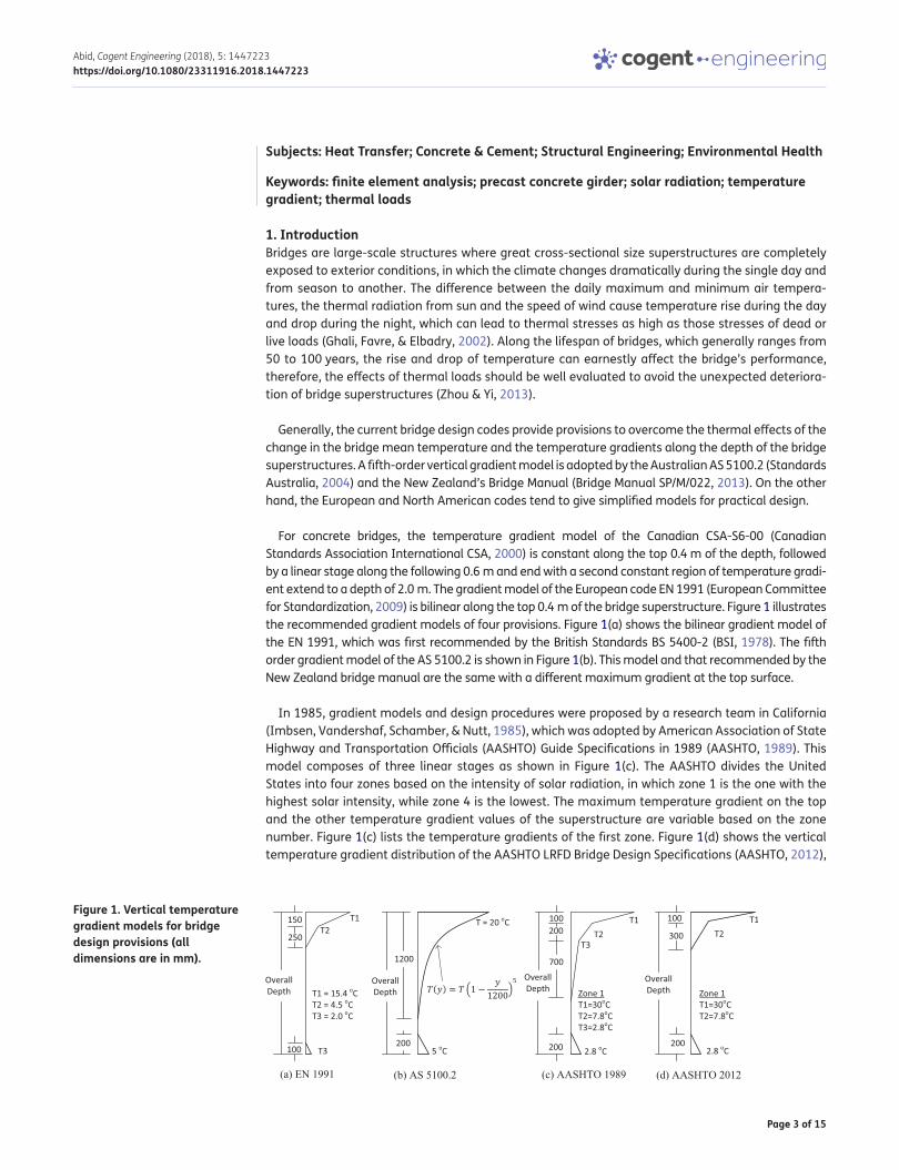
Generally, the current bridge design codes provide provisions to overcome the thermal effects of the change in the bridge mean temperature and the temperature gradients along the depth of the bridge superstructures. A fifth-order vertical gradient model is adopted by the Australian AS 5100.2 (Standards Australia, 2004) and the New Zealand’s Bridge Manual (Bridge Manual SP/M/022, 2013). On the other hand, the European and North American codes tend to give simplified models for practical design.

For concrete bridges, the temperature gradient model of the Canadian CSA-S6-00 (Canadian Standards Association International CSA, 2000) is constant along the top 0.4 m of the depth, followed by a linear stage along the following 0.6 m and end with a second constant region of temperature gradi-ent extend to a depth of 2.0 m. The gradient model of the European code EN 1991 (European Committee for Standardization, 2009) is bilinear along the top 0.4 m of the bridge superstructure. Figure 1 illustrates the recommended gradient models of four provisions. Figure 1(a) shows the bilinear gradient model of the EN 1991, which was first recommended by the British Standards BS 5400-2 (BSI, 1978). The fifth order gradient model of the AS 5100.2 is shown in Figure 1(b). This model and that recommended by the New Zealand bridge manual are the same with a different maximum gradient at the top surface.

In 1985, gradient models and design procedures were proposed by a research team in California (Imbsen, Vandershaf, Schamber, & Nutt, 1985), which was adopted by American Association of State Highway and Transportation Officials (AASHTO) Guide Specifications in 1989 (AASHTO, 1989). This model composes of three linear stages as shown in Figure 1(c). The AASHTO divides the United States into four zones based on the intensity of solar radiation, in which zone 1 is the one with the highest solar intensity, while zone 4 is the lowest. The maximum temperature gradient on the top and the other temperature gradient values of the superstructure are variable based on the zone number. Figure 1(c) lists the temperature gradients of the first zone. Figure 1(d) shows the vertical temperature gradient distribution of the AASHTO LRFD Bridge Design Specifications (AASHTO, 2012),

Figure 1. Vertical temperature gradient models for bridge design provisions (all dimensions are in mm).

Page 4 of 15

Abid, Cogent Engineering (2018), 5: 1447223https://doi.org/10.1080/23311916.2018.1447223

which is a simplified bilinear model derived from the one shown in Figure 1(c). In this model, the same zone division still adopted, also T1 and T2 have exactly the same values as those listed in the older gradient model.

Many field, experimental, and numerical studies have been conducted during the last three decades to enrich the knowledge about thermal loads effects on bridge girders and superstructures. In previ-ous works, the temperatures and temperature gradient distributions in concrete box-girders (Abid, Taysi, et al., 2016; Tayşi & Abid, 2015) and composite I-girders (Abid, Mussa, Tayşi, & Özakça, 2018) were investigated both experimentally and numerically using the theory of finite element. Lee (2010, 2012) conducted an experimental research on a precast concrete I-girder under the open-conditions in Atlanta, USA. Other experimental works were conducted on other types and configurations of bridge girders (Kulprapha & Warnitchai, 2012; Liu, Chen, & Zhou, 2012; Song, Xiao, & Shen, 2012; Wang, Zhan, & Zhao, 2016). On the other hand, significant numerical investigations were conducted during the last 3 years (Abid, Alrebeh, et al., 2016; El-Tayeb, El-Metwally, Askar, & Yousef, 2017; Jiao, Borchani, Hasni, & Lajenf, 2017; Krkoškaa & Moravčík, 2015; Zhou, Xia, Brownjohn, & Koo, 2016; Zhu & Meng, 2017).

The current paper aims to focus on the effect of solar radiation and air temperature variation in addition to the other thermal loads on temperature gradient distributions in concrete bridges with precast girders during the construction period. Two construction stages were studied, the isolated (single) precast girder before the casting of the deck slab and the precast girders-deck slab super-structure system before the application of topping layers. Finally, the temperature gradient distribu-tions calculated for extreme thermal loads were compared with the current AASHTO vertical gradient model shown in Figure 1(d).

2. Finite element modelingThe conduction of heat through the girder volume is governed by the Fourier heat transfer differen-tial equation,

In which ρ is the density, C is the specific heat, k is the thermal conductivity and ∇T is the gradient of the temperature T at any direction and Q represents the heat generated within the girder volume.

The sum of all heat flux exchanges on the surfaces of the girder in W/m2 is:

In which, hc is the convection coefficient in W/m2°C, qs is the solar radiation heat flux, α is the radia-tion absorptivity of the surface, qg is the radiation reflected from the surrounding ground and ob-jects, � is the surface emissivity, and σs is the Stefan-Boltzmann constant, while Ts and Ta are the surface and the air temperatures.

The first term represents the convection heat transfer on surfaces with the ambient air, while the second and third terms represent the thermal radiation heat flux received from the sun and re-flected from the bridge surroundings, respectively. The fourth term describes the re-radiation from the girder surfaces to the atmosphere.

To estimate the value of hc, the empirical formulas shown in Equation (3) (Duffie & Beckman, 2006) or Equation (4) (Larsson & Karoumi, 2011; Larsson & Thelandersson, 2011) can be used. In this paper the formula shown in Equation (5) (Lee, 2012) was used. In Equations (3)–(5), v represents the wind speed.

(1)�CdT

dt= ∇(k∇T) + Q

(2)q = hc(Ts − Ta) + �qs + �qg + ��s(T4

s − T4

a )

(3)hc = 5.7 + 3.8v

(4)hc = 6.0 + 4.0v (v ≤ 5m/s)

Page 5 of 15

Abid, Cogent Engineering (2018), 5: 1447223https://doi.org/10.1080/23311916.2018.1447223

In this study, an experimental precast concrete girder was analyzed under the effect of environmen-tal thermal loads. The girder was constructed by Lee (2010) and was instrumented with 28 surface and embedded thermocouples. Figure 2 shows the detail cross-sectional geometry of the tested girder segment and the locations of the instrumented 28 thermocouples (T1 through T28).

The thermal Finite Element (FE) analysis was conducted using the COMSOL Multiphysics FE pack-age (COMSOL Multiphysics v 4.3a, 2012). The density of the concrete, the specific heat and the ther-mal conductivity were defined in COMSOL as 2,400 kg/m3, 1,000 J/kg°C and 1.5 W/m°C, respectively (Lee, 2012). On the other hand, the surface emissivity � and the surface absorption coefficient α were 0.85 and 0.5, respectively.

The cross-sectional surfaces were considered isolated to model the longitudinal continuity of the girder. The thermal analysis was initiated three days before the required day with an initial tempera-ture equals the air temperature at 12:00 am To assure high accuracy of temperature calculations, fine mesh was used with more than 41,200 quadratic tetrahedral elements and more than 6,000 surface triangular elements. The analysis was conducted at time intervals of 10 min to better cap-ture the maximum variation of temperatures. All loads mentioned in Equation (2) were applied si-multaneously using different loading options. The solar radiation was applied using the COMSOL solar model, while the convection was applied using the convection loading option in which the wind speed was introduced as a time-dependent variable. The air temperature used in the convection and the re-radiation terms of Equation (2) was also defined as a time-dependent variable based on the experimental records. The ground reflected radiation was modeled as a heat flux based on the ex-perimental time-dependent solar radiation records.

3. Comparisons between FE and experimental temperaturesFigures 3 and 4 show comparisons between the FE predicted temperature distributions and the ex-perimental temperature distributions (Lee, 2010) along the depth of the web and the breadth of the top flange. The 24-h experimental records of air temperature, solar radiation and wind speed were considered in this FE thermal analysis. The comparisons were made based on the thermal loads and the experimental results of 15-November-2009. Two statistical tools were used to evaluate the pre-diction errors, the Average Absolute Difference (AAD) and the Maximum Absolute Difference (MAD). The AAD is the average of the absolute differences between the FE predicted temperatures (TFE) and the experimental temperatures (TEx), at specific time steps and for a specific group of thermocou-ples, which is given by,

(5)hc = 5.6 + 4.0v (v ≤ 5m/s)

Figure 2. Geometry of the precast girder and locations of thermocouples (all dimensions in mm).

Source: Lee (2010).

Page 6 of 15

Abid, Cogent Engineering (2018), 5: 1447223https://doi.org/10.1080/23311916.2018.1447223

On the other hand, the MAD is the maximum record absolute difference at any of the thermocouples within a group of thermocouples at a specific time step.

Figure 3(a) shows a comparison of the predicted and the experimental temperatures along the depth of the web at 7:40 am It is shown that there is a quite good agreement between the predicted and the experimental temperatures, and that difference reaches its minimum at T5 and T9, at which the absolute differences were 0.45 and 0.4 °C, respectively. The FE analysis was conducted at time steps of 10 min; therefore, the comparison of the experimental distribution at 1:05 pm was per-formed using the FE predicted temperature distribution at 1:00 pm.

It is clearly shown in Figure 3(b) that the FE predicted temperatures show better agreement with the experimental temperatures during the afternoon than during the morning hours. The tempera-ture differences at T28, T7 and the average of T12 and T13 at 1:00 pm were 0.4, 0.2 and 0.9 °C, re-spectively, while the corresponding temperature differences at 7:40 am were 1.1, 2.2 and 1.4, respectively. On the other hand, the FE temperature distribution at 12:10 pm, in which the time lag was 55 min, shows better agreement with the experimental distribution at 1:05 pm. The AAD at 12:10 pm was 1.1 °C, while at 1:00 pm it was 1.7 °C. The radiation in this period of the year is gener-ally of low altitude angles. On the other hand, the solar radiation altitude angles are significantly low during the early morning hours. Such low angles increase the shading projection lengths of the sur-rounding buildings and objects. Therefore, the temperature difference shown in Figure 3(a) at T7 can

(6)AAD =

∑��TFE − TEx

��n

Figure 3. Comparison of the experimental and the FE temperature distributions along the depth of the web.

8 12 16 20

Temperature (oC)

0

0.2

0.4

0.6

0.8

1

1.2

1.4

1.6

Web

Hei

ght (

m)

EXP 7:40 a.m.FE 7:40 a.m.

Maximum DifferenceAt thermocouple

T7 (2.2 oC)

10 15 20 25 30 35

Temperature (oC)

0

0.2

0.4

0.6

0.8

1

1.2

1.4

1.6

Web

Hei

ght (

m)

EXP 1:05 p.m.FE 1:00 p.m.FE 12:10 p.m.

Figure 4. Comparison of the experimental and the FE temperature distributions along the width of the top flange.

-0.5 -0.4 -0.3 -0.2 -0.1 0 0.1 0.2 0.3 0.4 0.5

Top Flange Width (m)

6

8

10

12

14

Tem

pera

ture

(o C)

EXP 7:40 amFE 7:40 am

(a)

-0.5 -0.4 -0.3 -0.2 -0.1 0 0.1 0.2 0.3 0.4 0.5

Top Flange Width (m)

16

20

24

28

32

36

Tem

pera

ture

(o C)

EXP 1:45 pmFE 1:40 pmFE 12:50 pm

(b)

Page 7 of 15

Abid, Cogent Engineering (2018), 5: 1447223https://doi.org/10.1080/23311916.2018.1447223

be attributed to the full or partial shading of this part during the shining hours before 7:40 am However, a 2.2 °C is an acceptable maximum difference.

The difference between the predicted and the experimental temperatures along the width of the top flange at 7:40 am ranged from 0.15 to 0.45 °C as shown in Figure 4(a), which reflects the high adequacy of the current FE model. Figure 4(b) shows a comparison between the experimental tem-peratures along of the top flange at 1:45 pm and the FE predicted temperatures at 1:40 pm (with 5 min time lag) and 12:50 pm (with 55 min time lag). The temperature difference ranged from 0.3 °C to 2.4 °C at 1:40 pm, and from 0.3 °C to 1.9 °C at 12:50 pm. Solar radiation becomes the daily highest during the mid-day hours. As sun strikes at the highest daily altitude angles during this period, the most effective solar radiation budget is received by the top surface of the girded. Consequently, the temperature of the top flange would be increased obviously during the mid-day hours. This increase, when taking into account the effect of the possible fluctuation of the cloud cover, may increase the differences between the recorded and predicted temperatures during the noon hours. The details of AAD and MAD are listed in Table 1. The AAD for all the compared temperature distributions and at all the compared time steps ranged from 0.2 to 1.8 °C. Moreover, the MAD ranged from 0.4 to 2.9 °C. Thus, the current FE model agrees well with the experimental results.

4. Temperature-time curvesTo present the effect of air temperature change and solar radiation on concrete bridges, a hot sum-mer day was chosen. Environmental data including air temperature and solar radiation were col-lected from a weather station installed specially for this purpose on the campus of Gaziantep University, Turkey. June 2 was found to be the day with the highest solar radiation among the re-cords of summer, 2013. The maximum hourly solar radiation incidence on June 2 was 1,200 W/m2. To evaluate the extreme change of temperature, the recorded minimum temperature of June 2, 2013, which equals 12 °C, was adopted together with the maximum record temperature from a 30 years history, the maximum temperature of June 2 for the period from 1980 to 2013 is 38 °C. To evaluate the extreme case, the wind speed was considered zero.

Figure 5(a) shows the temperature-time curves for six thermocouples on June 2, which were se-lected to represent the 28 thermocouples. Three surface thermocouples, T28, T12 and T20, and three core thermocouples, T5, T9 and T7. It is clear that T28 on the top surface exhibited the highest

Table 1. AAE and MAE of the web and the top flangeWeb Top Flange

7:40 am 12:10 pm 1:00 pm 7:40 am 12:50 pm 1:40 pmAAD (°C) 1.1 1.1 1.6 0.2 0.9 1.8

MAD (°C) 2.2 1.7 2.9 0.4 1.9 2.4

Time lag (min) 0 55 5 0 55 5

Figure 5. Temperature-time curves on June 2 (a) for different thermocouples and (b) for the maximum, minimum and average temperatures of the girder.

15

25

35

45

55

65

Tem

pera

ture

(oC

)

T28- Top surfaceT12- Bottom surfaceT20- Web surfaceT5- TF coreT9- BF coreT7- Web core

0 3 6 9 12 15 18 21 24

Time (hr)

(a)

0 3 6 9 12 15 18 21 24

Time (hr)

10

20

30

40

50

60

70

Tem

pera

ture

(oC

)

Tmax

Tave

Tmin

Max. difference32.6oC at 1:50 pm

Min. difference10.4oC at 7:40 am

Min. Temperature15.2oC at 4:40 am

Max. Temperature64.7oC at 2:50 pm

(b)

Page 8 of 15

Abid, Cogent Engineering (2018), 5: 1447223https://doi.org/10.1080/23311916.2018.1447223

altitude with a maximum temperature of 59 °C around 3:00 pm. Although T5, is not a surface ther-mocouple (installed 45 mm below T28) it showed the second highest temperature among the six thermocouples. This is due to the high solar radiation flux absorbed by the top surface during the day hours. The maximum temperature of T5 was about 54.7 °C, which occurred at approximately 5:00 pm. The low thermal conductivity of concrete explains the two hours delay of T5’s maximum temperature.

T9 is the thermocouple surrounded by the largest concrete mass, for this reason it exhibited the highest temperatures during the cold hours (from midnight to sunrise) and the lowest temperatures during the hot midday hours. The behavior of T9 can simply be attributed to the thermal conductiv-ity/concrete cover ratio. The conductivity of concrete is only 1.5 W/m°C, while the concrete surround-ing T9 is the thicker compared to the other thermocouples. The temperature distribution of T7 (at the core of the web) tried to follow the behavior of T9, however, it was more affected by surface heating and cooling due its lower surrounding concrete cover. The bottom surface thermocouple T12 seemed to have the same behavior of T28 but with a lower altitude along the 24 h, the maximum tempera-ture of T12 around 3:00 pm was 47.6 °C.

Figure 5(b) shows the hourly maximum, minimum and average temperatures of the girder during the 24 h. It is clear that the behavior of the maximum bridge temperature differs from that of the minimum bridge temperature. The altitude of the maximum bridge temperature showed higher variation than that of minimum temperature, moreover, the times of extremes were different. The maximum bridge temperature occurred at 2:50 pm, which was 64.7 °C, while the minimum was 15.2 °C at 4:40 am

The minimum temperature distribution showed its minimum before that of the maximum tem-perature distribution by approximately 50 min, while reached its maximum, which was 38.9 °C at 5:30 pm, hence, 160 min after the maximum of the maximum temperature distribution. Thus, the maximum bridge temperature was much higher affected by the fluctuation of air temperature and solar radiation than the minimum temperature of the bridge. Because of these different behaviors, the in-time temperature difference (between the maximum and minimum temperatures) was vari-able with time, which reached a maximum of 32.6 °C at 1:50 pm and a minimum of 10.4 °C at 7:40 am as shown in Figure 5(b). On the other hand, the average bridge temperature varied between 21.9 °C at 5:20 am and 45.6 °C at 4:40 pm.

5. Vertical and lateral temperature gradientsThe temperature gradients along the depth of the girder are shown in Figure 6 for different time steps. In general, the girder’s temperature at 4:00 am was the coldest along the whole day, further-more, the temperature gradient was negative at this time, at which the temperature of the top and bottom surface was colder than of concrete interiors. The maximum temperature at this time step occurred at T9, while the temperatures of the top surface and lower surface were lower than at T9 by 6.1 °C and 5.8 °C, respectively. The temperature gradient at 8:00 pm shows that the gradient tended to be negative during the early night hours, but with different temperature distribution. During the hot day hours, the temperature of girder increased significantly. Moreover, the tempera-ture of top surface became much higher than the temperature of interiors as illustrated for tempera-ture gradients at 2:10 pm and 5:00 pm in Figure 6. The recorded maximum vertical temperature gradient was 26.3 °C, which occurred at 2:10 pm as shown in Figure 6.

Figure 7(a) shows the temperature gradients along the top flange at three different time steps. The temperature at 1:20 pm was the highest along the whole width of the top flange with an aver-age temperature exceeding 50 °C, while the maximum gradient at this time step, which occurred in the southern face of the flange, was 7.6 °C as shown in Figure 7(a). After hours of convection cooling and with the absence of heating loads (solar radiation and hot air temperature), the temperature of the top flange decreased significantly to reach an average of about 26 °C at 1:10 am The maximum negative gradient at 1:10 am was found to be higher than the maximum positive gradient at 1:20 pm.

Page 9 of 15

Abid, Cogent Engineering (2018), 5: 1447223https://doi.org/10.1080/23311916.2018.1447223

The maximum negative gradient at the southern face of the top flange was recorded to be 10.8 °C as shown in Figure 7(a). The temperature distribution at 9:20 am seems to be uniform along the whole width of the top flange, recording the lowest daily temperature gradient, which was 1.4 °C only.

Figure 7(b) shows that the temperature gradients along the bottom flange differ from those of the top flange. It seems that the daytime heating affected the edges of the bottom flange (especially the south edge) without causing serious heating of the bottom flange’s center, which contrasts the semi uniform heating of the top surface of the top flange. The configuration of the girder, hence the different periods and amounts of exposure to solar radiation interpret the different behaviors of the top and the bottom flanges. The high difference of solar exposure between the edges and the center of the bottom flange magnifies its temperature gradient, which was about 24 °C (1:30 pm) as shown in Figure 7(b). On the other hand, the maximum negative temperature occurred at 1:10 am and was 10.7 °C.

The average temperature of the bottom flange increased during the late hours of the day because sunrays during these hours strike at lower altitudes, thus reaching the whole area of the bottom surface. In this time of the year, the sun moves completely to the south of the equator. Hence, it rises from south-east and sets at south-west. Therefore, the southern edge of the bottom flange is com-pletely subjected to direct solar heating during the shining hours, while the northern edge is com-pletely shaded. This explains the sharp temperature rise shown at the southern edge in Figure 7(b).

Figure 6. Temperature gradients along the depth of the girder at different times.

-10 -5 0 5 10 15 20 25 30

Temperature Gradient(oC)

0

0.2

0.4

0.6

0.8

1

1.2

1.4

1.6

Web

Hei

ght (

m)

4:00 am2:10 pm5:00 pm8:00 pm

Figure 7. Temperature gradients at different time steps along (a) the top flange and (b) the bottom flange.

-0.6 -0.4 -0.2 0 0.2 0.4 0.6

Top Flange Width (m)

-15

-10

-5

0

5

10

15

Tem

pera

ture

Gra

dien

t (o C

)

1:10 am9:20 am1:20 pm

(a)

-0.4 -0.3 -0.2 -0.1 0 0.1 0.2 0.3 0.4

Bottom Flange Width (m)

-15

-10

-5

0

5

10

15

20

25

Tem

pera

ture

Gra

dien

t (o C

)

1:10 am7:50 pm1:30 pm

(b)

Page 10 of 15

Abid, Cogent Engineering (2018), 5: 1447223https://doi.org/10.1080/23311916.2018.1447223

Such obvious difference is not shown in the top flange as shown in Figure 7(b). This is because of the direct solar heating of the top surface of the top flange, which reduces the differences between the two edges.

The average temperature of the bottom flange at 7:50 pm was 40.3 °C, which is higher than at 1:30 pm. Furthermore, the temperature of bottom flange at this time step was more stable than other time steps, with the minimum temperature gradient of about 5 °C as shown in Figure 7(b).

6. Modeling of the girders-deck slab superstructure

6.1. Geometry and modelingIn this section, the temperature distributions and gradients are discussed for a completed super-structure, which composes of a series of precast concrete girders and a concrete deck slab, but be-fore the topping with asphalt layers. Figure 8 illustrates the geometry of the modeled superstructure, which composes of three girders (same dimensions and properties as that given in Figure 2) and a 200 mm thickness deck slab. One interior girder can model all interior girders, while the edge girders should be modeled. Therefore, to reduce the calculation time, the superstructure was reduced to that shown in Figure 8 with a center-to-center girder spacing of 2.1 m.

To simulate the actual case where sunrays do not reach the interior surfaces of the girders or the lower surface of the slab deck, these surfaces were modeled to receive no solar radiation. In con-trast, the exterior surfaces of edge girders, the bottom surfaces of all girders, the lower and the verti-cal surfaces of the cantilever portions and the top surface of the deck slab were considered as exposed surfaces. Nevertheless, reflected radiation from the ground was calculated for all lower, inclined and vertical surfaces.

6.2. Temperature distributionsDue to the different distribution of thermal loads, the temperature distributions in the bridge super-structure differ from those in the single girder. Figure 9 shows the three-dimensional temperature distributions in the bridge superstructure before sunrise (at 5:00 am) where the bridge temperature was the minimum and at the time of the maximum bridge temperature (3:10 pm). As it is clear in Figure 9(b), sunrays do not strike the interior surfaces of girders, while as shown the other surfaces are directly exposed to solar radiation. Likewise, it is obvious that the shadowing effects from canti-lever portions led to lower heating loads at the exterior surface of edge girders. Due to its direct and almost continuous exposure to sun rays along the daytime, the top surface exhibited a semi uniform temperature, which was the maximum of the superstructure. Due to the low absorbed solar radia-tion fluxes, the cores of the bottom flanges showed the lowest temperature during the day hours as shown in Figure 9(b). On the other hand and as shown in Figure 9(a), the cores of the top flanges stored larger amounts of heat after the long cooling hours of the night. This is because the higher absorbed radiation heat via the top surface of the slab during day hours and because of the large volumes of concrete surrounding these cores.

Figure 8. Geometry of the modeled bridge superstructure.

Page 11 of 15

Abid, Cogent Engineering (2018), 5: 1447223https://doi.org/10.1080/23311916.2018.1447223

6.3. Vertical temperature gradientsFigure 10 shows a comparison between the maximum vertical temperature gradients of the mod-eled superstructure and the single girder. It is shown that the depth of the superstructure is 200 mm deeper, which is the thickness of the deck slab. The temperature gradient along the web centerline of the interior girder is presented in Figure 10, which was chosen to represent the superstructure because it was the highest one. The maximum temperature gradient of the interior girder was 32.6 °C, while the maximum temperature gradients of both the southern and the northern girders were about 29.9 °C. The interior girder was exposed to solar radiation from the top and the bottom surfaces only, while the webs of edge girders were also exposed to solar radiation. Thus, the tem-peratures of the web and the bottom flange of the interior girder were lower than of edge girders, which explain the higher temperature gradients between the top surface and the concrete interiors along the interior girder.

It is shown in Figure 10 that the maximum temperature gradients of the superstructure on both the top and the bottom surfaces were higher than those of the single girder, while in both cases, the zero-gradient occurred in the core of the bottom flange. The maximum temperature gradient of the single girder was 26.3 °C, while that of the superstructure was 32.6 °C, with a percentage increase of 24%. The gradients at the bottom surface were 6.0 °C and 8.6 °C for the single girder and the super-structure, respectively, with a percentage increase of about 24%.

Figure 9. Three-dimensional temperature distributions in the bridge superstructure at (a) 5:00 am and (b) 3:10 pm.

Figure 10. Vertical temperature gradients of the superstructure and the single girder.

0 5 10 15 20 25 30 35

Temperature Gradient (oC)

1.8

1.6

1.4

1.2

1

0.8

0.6

0.4

0.2

0

Web

Hei

ght (

m)

Superstructure 1:50 pmSingle Girder 2:10 pm

Page 12 of 15

Abid, Cogent Engineering (2018), 5: 1447223https://doi.org/10.1080/23311916.2018.1447223

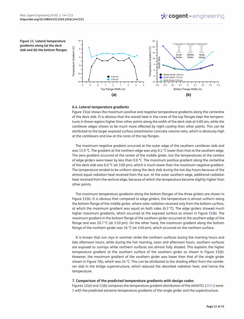
6.4. Lateral temperature gradientsFigure 11(a) shows the maximum positive and negative temperature gradients along the centerline of the deck slab. It is obvious that the stored heat in the cores of the top flanges kept the tempera-tures in these regions higher than other points along the width of the deck slab at 4:00 am, while the cantilever edges shown to be much more affected by night cooling than other points. This can be attributed to the larger exposed surface area/interior concrete volume ratio, which is obviously high at the cantilevers and low at the cores of the top flanges.

The maximum negative gradient occurred at the outer edge of the southern cantilever slab and was 13.9 °C. The gradient at the northern edge was only 0.2 °C lower than that at the southern edge. The zero-gradient occurred at the center of the middle girder, but the temperatures at the centers of edge girders were lower by less than 0.6 °C. The maximum positive gradient along the centerline of the deck slab was 6.0 °C (at 3:00 pm), which is much lower than the maximum negative gradient. The temperature tended to be uniform along the deck slab during the hot day hours because of the almost equal radiation heat received from the sun. At the outer southern edge, additional radiation heat received from the vertical edge, because of which the temperature became slightly higher than other points.

The maximum temperature gradients along the bottom flanges of the three girders are shown in Figure 11(b). It is obvious that compared to edge girders, the temperature is almost uniform along the bottom flange of the middle girder, where solar radiation received only from the bottom surface, at which the maximum gradient was equal on both sides (6.3 °C). The edge girders showed much higher maximum gradients, which occurred at the exposed surface as shown in Figure 11(b). The maximum gradient in the bottom flange of the southern girder occurred at the southern edge of the flange and was 20.7 °C (at 3:10 pm). On the other hand, the maximum gradient along the bottom flange of the northern girder was 16 °C (at 3:40 pm), which occurred on the northern surface.

It is known that sun rays in summer strike the northern surfaces during the morning hours and late afternoon hours, while during the hot morning, noon and afternoon hours, southern surfaces are exposed to sunrays while northern surfaces are almost fully shaded. This explains the higher temperature gradient at the southern surface of the southern girder as shown in Figure 11(b). However, the maximum gradient of the southern girder was lower than that of the single girder shown in Figure 7(b), which was 24 °C. This can be attributed to the shading effect from the cantile-ver slab in the bridge superstructure, which reduced the absorbed radiation heat, and hence the temperature.

7. Comparison of the predicted temperature gradients with design codesFigures 12(a) and 12(b) compares the temperature gradient distribution of the AASHTO, (2012) zone-1 with the predicted extreme temperature gradients of the single girder and the superstructure.

Figure 11. Lateral temperature gradients along (a) the deck slab and (b) the bottom flanges.

-4 -3 -2 -1 0 1 2 3 4

Top Flange Width (m)

-15

-10

-5

0

5

10

Tem

pera

ture

Gra

dien

t (o C

)4:00 am3:00 pm

(a)

-0.4 -0.3 -0.2 -0.1 0 0.1 0.2 0.3 0.4

Bottom Flange Width (m)

-10

-5

0

5

10

15

20

25

Tem

pera

ture

Gra

dien

t (o C

)

Middle Girder 3:20 pmSouth Girder 3:10 pmNorth Girder 3:40 pm

Sout

h fa

ce

MiddleGirder

SouthGirder

NorthGirder

(b)

Page 13 of 15

Abid, Cogent Engineering (2018), 5: 1447223https://doi.org/10.1080/23311916.2018.1447223

The comparison focuses on four points; the maximum temperature gradient at the top surface, the gradient distribution along the top region of the girder and the superstructure, the gradient dis-tribution along the web and the maximum temperature gradient at the bottom surface. Figure 12(a) shows well agreement between the AASHTO’s and the single girder’s gradients along the top region and along the web, however, AASHTO slightly overestimated the gradient at the top surface and underestimated the gradient at the bottom surface. The difference was less than 4 °C at the top and the bottom surfaces. As shown in Figure 12(a), the deviation along the top region (the top 0.4 m) was less 3 °C, while the maximum deviation along the web was 2.3 °C.

The gradient distribution of the superstructure showed a higher deviation from the AASHTO gradi-ent distribution compared to the single girder as shown in Figure 12(b) both in the top region and along the web. The single girder showed semi-constant gradient along the web, with a maximum deviation of approximately 1.5 °C, while the maximum deviation of the temperature gradients of the superstructure along the web was approximately 4 °C. Furthermore, the AASHTO’s gradient model underestimated the maximum temperature gradient at the top surface and the bottom surface by 2.6 °C and 5.8 °C, respectively.

8. ConclusionsBased on a three-dimensional FE thermal analysis, the effect of solar radiation and climate daily change on precast girders-deck slab concrete bridges was studied. In this paper, the single girder and the girders-deck slab superstructure before applying topping layers were investigated, which are the two stages of the construction of such types of bridges. The temperature gradients were in-vestigated for the case of the extreme summer thermal loads and compared with the current AASHTO provisions. Within the limits of the included parameters in this study, the followings can be concluded:

The top surface exhibited the highest temperature during the day; the maximum temperature of T28 was 59 °C at 3:00 pm, while its temperature was close to the lowest temperature during the early morning. In contrast, the temperature of the core of the bottom flange was the highest during the cold hours and the lowest during the peak temperature hours. These two opposite behaviors are attributed to the thickness of the surrounding concrete and the low thermal conductivity of con-crete. The hourly difference between the bridge’s maximum and minimum temperatures varied sig-nificantly during the day. The maximum predicted temperature difference was 32.6 °C at 1:50 pm, while the minimum was 10.4 °C at 7:40 am

Figure 12. Comparison of the predicted temperature gradients with AASHTO’s gradient (a) the single girder and (b) the superstructure.

Temperature Gradient (oC)

0

0.2

0.4

0.6

0.8

1

1.2

1.4

1.6

Web

Hei

ght (

m)

Single GirderCurrent StudyAASHTO

(a)

0 5 10 15 20 25 30 0 5 10 15 20 25 30 35

Temperature Gradient (oC)

0

0.2

0.4

0.6

0.8

1

1.2

1.4

1.6

1.8

Web

Hei

ght (

m)

SuperstructureCurrent StudyAASHTO

(b)

Page 14 of 15

Abid, Cogent Engineering (2018), 5: 1447223https://doi.org/10.1080/23311916.2018.1447223

The maximum predicted vertical temperature gradient of the single girder was 26.3 °C, while the maximum vertical temperature gradient of the superstructure along the centerline of the web of the interior girder was 32.6 °C, while it was approximately 29 °C for the edge girders. The web shading from the cantilever slab reduced the web temperature of southern edge girder compared to the single girder, because of which, the maximum lateral gradient along the bottom flange of the single girder was higher by about 3 °C. Comparing with the current AASHTO’s vertical temperature gradient model (zone 1), the predicted extreme gradient distribution of the single girder showed good agree-ment, however, the AASHTO’s model overestimated the gradient at the top surface by approximate-ly 4 °C. On the other hand, the AASHTO’s gradient model underestimated the maximum temperature gradient at the top surface by 2.6 °C.

FundingThe author received no direct funding for this research.

Author detailsSallal R. Abid1

E-mails: sallal@uowasit.edu.iq, sallalsallal@yahoo.comORCID ID: http://orcid.org/0000-0002-4023-73821 Department of Civil Engineering, University of Wasit, Kut,

Iraq.

Citation informationCite this article as: Three-dimensional finite element temperature gradient analysis in concrete bridge girders subjected to environmental thermal loads, Sallal R. Abid, Cogent Engineering (2018), 5: 1447223.

Cover imageSource: Author.

ReferencesAASHTO. (1989). AASHTO guide specifications: Thermal effects

in concrete bridge superstructures. Washington, DC: Author.

AASHTO. (2012). AASHTO LRFD bridge design specifications. Washington, DC: Author.

Abid, S. R., Alrebeh, S., Tayşi, N., & Özakça, M. (2016). Finite element thermal analysis of deep box-girders. International Journal of Civil Engineering and Technology, 7, 128–139.

Abid, S. R., Mussa, F., Tayşi, N., & Özakça, M. (2018). Experimental and finite element investigation of temperature distributions in concrete-encased steel girders. Structural Control and Health Monitoring, 25, 1–23. in press. doi:10.1002/stc.2042

Abid, S. R., Tayşi, N., & Özakça, M. (2016). Experimental analysis of temperature gradients in concrete box girders. Construction and Building Materials, 106, 523–532. doi:10.1016/j.conbuildmat.2015.12.144

AS 5100.2. (2004). Bridge design-part 2: Design loads. Sydney: Standards Australia.

Bridge Manual SP/M/022. (2013). Section 3: Design loading. Wellington: NZ Transport Agency.

BS 5400: Part2. (1978). Steel concrete and composite bridges. Specifications for loads. London: British Standards Institution.

CAN/CSA-S6-00. (2000). Canadian highway bridge design code. Toronto: Canadian Standards Association International.

COMSOL Multiphysics v 4.3a. (2012). Heat transfer module user’s guide. Stockholm: COMSOL.

Duffie, J. A., & Beckman, W. A. (2006). Solar engineering of thermal processes. Hoboken, NJ: John Wiley and Sons Inc.

El-Tayeb, E. H., El-Metwally, S. E., Askar, H. S., & Yousef, A. M. (2017). Thermal analysis of reinforced concrete beams and frames. HBRC Journal, 13, 8–24. doi:10.1016/j.hbrcj.2015.02.001

EN 1991-1-5:2003. (2009). Eurocode 1: Actions on structures-part 1-5: General actions-thermal actions. European Committee for Standardization.

Ghali, A., Favre, R., & Elbadry, M. (2002). Concrete structures stresses and deformations. London: Spon Press.

Imbsen, R. A., Vandershaf, D. E., Schamber, R. A., & Nutt, R. V. (1985). Thermal effects in concrete bridge superstructures. National Cooperative Highway Research Program Report 276. Washington, DC: Transportation Research Board.

Jiao, P., Borchani, W., Hasni, H., & Lajenf, N. (2017). A new solution of measuring thermal response of prestressed concrete bridge girders for structural health monitoring. Measurement Science and Technology, 28, 1–11. doi:10.1088/1361-6501/aa6c8e

Krkoškaa, L., & Moravčík, M. (2015). The analysis of thermal effect on concrete box girder bridge. Procedia Engineering, 111, 470–477. doi:10.1016/j.proeng.2015.07.118

Kulprapha, N., & Warnitchai, P. (2012). Structural health monitoring of continuous prestressed concrete bridges using ambient thermal responses. Engineering Structures, 40, 20–38. doi:10.1016/j.engstruct.2012.02.001

Larsson, O., & Karoumi, R. (2011). Modeling of climatic thermal actions in hollow concrete box cross-sections. Structural Engineering International, 21, 74–79. doi:10.2749/101686611X12910257102550

Larsson, O., & Thelandersson, S. (2011). Estimating extreme values of thermal gradients in concrete structures. Materials and Structures, 44, 1491–1500. doi:10.1617/s11527-011-9714-0

Lee, J.-H. (2010). Experimental and analytical investigations of the thermal behavior of prestressed concrete bridge girders including imperfections (PhD Thesis 2010). Georgia Institute of Technology, Atlanta, p. 265.

Lee, J.-H. (2012). Investigation of extreme environmental conditions and design thermal gradients during construction for prestressed concrete bridge girders. Journal of Bridge Engineering, 17, 547–556. doi:10.1061/(ASCE)BE.1943-5592.0000277

Liu, H., Chen, Z., & Zhou, T. (2012). Theoretical and experimental study on the temperature distribution of h-shaped steel members under solar radiation. Applied Thermal Engineering, 37, 329–335. doi:10.1016/j.applthermaleng.2011.11.045

Song, Z., Xiao, J., & Shen, L. (2012). On temperature gradients in high-performance concrete box girder under solar radiation. Advances in Structural Engineering, 15, 399–415. doi:10.1260/1369-4332.15.3.399

Tayşi, N., & Abid, S. R. (2015). Temperature distributions and variations in concrete box-girder bridges: Experimental and finite element parametric studies. Advances in Structural Engineering, 18, 469–486. doi:10.1260/1369-4332.18.4.469

Page 15 of 15

Abid, Cogent Engineering (2018), 5: 1447223https://doi.org/10.1080/23311916.2018.1447223

© 2018 The Author(s). This open access article is distributed under a Creative Commons Attribution (CC-BY) 4.0 license.You are free to: Share — copy and redistribute the material in any medium or format Adapt — remix, transform, and build upon the material for any purpose, even commercially.The licensor cannot revoke these freedoms as long as you follow the license terms.

Under the following terms:Attribution — You must give appropriate credit, provide a link to the license, and indicate if changes were made. You may do so in any reasonable manner, but not in any way that suggests the licensor endorses you or your use. No additional restrictions You may not apply legal terms or technological measures that legally restrict others from doing anything the license permits.

Cogent Engineering (ISSN: 2331-1916) is published by Cogent OA, part of Taylor & Francis Group. Publishing with Cogent OA ensures:• Immediate, universal access to your article on publication• High visibility and discoverability via the Cogent OA website as well as Taylor & Francis Online• Download and citation statistics for your article• Rapid online publication• Input from, and dialog with, expert editors and editorial boards• Retention of full copyright of your article• Guaranteed legacy preservation of your article• Discounts and waivers for authors in developing regionsSubmit your manuscript to a Cogent OA journal at www.CogentOA.com

Wang, Y., Zhan, Y., & Zhao, R. (2016). Analysis of thermal behaviour on concrete box-girder arch bridges under convection and solar radiation. Advances in Structural Engineering, 19, 1043–1059. doi:10.1177/1369433216630829

Zhou, G. D., & Yi, T. H. (2013). Thermal loads in large-scale bridges: A state-of-the-art review. International Journal of Distributed Sensor Networks, 2013, 1–17. doi:10.1155/2013/217983

Zhou, L., Xia, Y., Brownjohn, J. M. W., & Koo, K. Y. (2016). Temperature analysis of a long-span suspension bridge based on field monitoring and numerical simulation. ASCE Journal of Bridge Engineering, 21, 1–10. doi:10.1061/(ASCE)BE.1943-5592.0000786

Zhu, J., & Meng, Q. (2017). Effective and fine analysis for temperature effect of bridges in natural environments. ASCE Journal of Bridge Engineering, 22, 1–19. doi:10.1061/(ASCE)BE.1943-5592.0001039