Embed Size (px)
Citation preview

One-Dimensional Finite Elements
An Introduction to the FE Method
Bearbeitet vonAndreas Öchsner, Markus Merkel
1. Auflage 2012. Buch. xxiv, 400 S. HardcoverISBN 978 3 642 31796 5
Format (B x L): 15,5 x 23,5 cmGewicht: 795 g
Weitere Fachgebiete > Technik > Maschinenbau Allgemein > Konstruktionslehre,Bauelemente, CAD
Zu Inhaltsverzeichnis
schnell und portofrei erhältlich bei
Die Online-Fachbuchhandlung beck-shop.de ist spezialisiert auf Fachbücher, insbesondere Recht, Steuern und Wirtschaft.Im Sortiment finden Sie alle Medien (Bücher, Zeitschriften, CDs, eBooks, etc.) aller Verlage. Ergänzt wird das Programmdurch Services wie Neuerscheinungsdienst oder Zusammenstellungen von Büchern zu Sonderpreisen. Der Shop führt mehr
als 8 Millionen Produkte.
Chapter 2Motivation for the Finite Element Method
Abstract The approach to the finite element method can be derived from differentmotivations. Essentially there are three ways:
• a rather descriptive way, which has its roots in the engineering working method,• a physical or• mathematically motivated approach.
Depending on the perspective, different formulations result, which however allresult in a common principal equation of the finite element method. The differentformulations will be elaborated in detail based on the following descriptions:
• matrix methods,• physically based working and energy methods and• weighted residual method.
The finite element method is used to solve different physical problems. Here solelyfinite element formulations related to structural mechanics are considered [1, 5–7,9–12].
2.1 From the Engineering Perspective Derived Methods
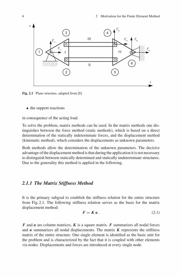
Matrix methods can be regarded in elastostatics as the initial point for the applicationof the finite element method to analyze complex structures [2, 3]. As example a planestructure can be given (see Fig. 2.1). This example is adapted from [8].
The structure consists of various substructures I, II, III and IV. The substructures arereferred to as elements. The elements are coupled at the nodes 2, 3, 4 and 5. Theentire structure is supported on nodes 1 and 6, an external load affects node 4.
Unknown are
• the displacement and reaction forces on every single inner node and
A. Öchsner and M. Merkel, One-Dimensional Finite Elements, 5DOI: 10.1007/978-3-642-31797-2_2, © Springer-Verlag Berlin Heidelberg 2013
6 2 Motivation for the Finite Element Method
Fig. 2.1 Plane structure, adapted from [8]
• the support reactions
in consequence of the acting load.
To solve the problem, matrix methods can be used. In the matrix methods one dis-tinguishes between the force method (static methods), which is based on a directdetermination of the statically indeterminate forces, and the displacement method(kinematic method), which considers the displacements as unknown parameters.
Both methods allow the determination of the unknown parameters. The decisiveadvantage of the displacement method is that during the application it is not necessaryto distinguish between statically determined and statically undeterminate structures.Due to the generality this method is applied in the following.
2.1.1 The Matrix Stiffness Method
It is the primary subgoal to establish the stiffness relation for the entire structurefrom Fig. 2.1. The following stiffness relation serves as the basis for the matrixdisplacement method:
F = K u . (2.1)
F and u are column matrices, K is a square matrix. F summarizes all nodal forcesand u summarizes all nodal displacements. The matrix K represents the stiffnessmatrix of the entire structure. One single element is identified as the basic unit forthe problem and is characterized by the fact that it is coupled with other elementsvia nodes. Displacements and forces are introduced at every single node.

2.1 From the Engineering Perspective Derived Methods 7
To solve the entire problem
• the compatibility and
• the equilibrium
have to be fulfilled.
In the matrix displacement method one introduces the nodal displacements as es-sential unknowns. The displacement vector at a node is defined to be valid for allelements connected at this node. Therewith the compatibility of the entire structurea priori is fulfilled.
A Single Element
Forces and displacements are introduced for each node of the single element(see Fig. 2.2).
Fig. 2.2 Single element (e) with displacements and forces
For an entirely obvious representation the nodal forces and the nodal displacementsare provided with an index ‘p’ to highlight that these are parameters, which aredefined on nodes. The vectors of the nodal displacements up or alternatively nodalforces Fp in general consist of various components for the respective coordinates.An additional index ‘e’ indicates to which element the parameters relate.1 Therewiththe nodal forces result, according to Fig. 2.2, in
1 The additional index ‘e’ is to be dropped at displacements since the nodal displacement is identicalfor each linked element in the displacement method.

8 2 Motivation for the Finite Element Method
Fei =
[Fix
Fiy
], Fe
j =[
Fj x
Fjy
], Fe
m =[
Fmx
Fmy
], (2.2)
and the nodal displacements in
ui =[
uix
uiy
], u j =
[u j x
u jy
], um =
[umx
umy
]. (2.3)
If one summarizes all nodal forces and nodal displacements at one element, the
entire node force vector Fep =
⎡⎣ Fi
F j
Fm
⎤⎦ (2.4)
as well as the
entire node displacement vector up =⎡⎣ ui
u j
um
⎤⎦ (2.5)
for a single element is described. With the vectors for the nodal forces and displace-ments the stiffness relation for a single element can be defined as follows:
Fep = ke up , (2.6)
or alternatively for each node:
Fer = ke
rs us (r, s = i, j,m) . (2.7)
The single stiffness matrix ke connects the nodal forces . In the present example thesingle stiffness relation is formally defined as
⎡⎢⎢⎢⎢⎢⎢⎢⎢⎢⎢⎢⎢⎣
Fix
Fiy
Fj x
Fjy
Fmx
Fmy
⎤⎥⎥⎥⎥⎥⎥⎥⎥⎥⎥⎥⎥⎦
=
⎡⎢⎢⎢⎢⎢⎢⎢⎢⎢⎢⎢⎢⎢⎣
kei i ke
i j keim
kej i ke
j j kejm
kemi ke
mj kemm
⎤⎥⎥⎥⎥⎥⎥⎥⎥⎥⎥⎥⎥⎥⎦
⎡⎢⎢⎢⎢⎢⎢⎢⎢⎢⎢⎢⎢⎣
uix
uiy
u j x
u jy
umx
umy
⎤⎥⎥⎥⎥⎥⎥⎥⎥⎥⎥⎥⎥⎦
. (2.8)
For further progression it needs to be assumed that the single stiffness matrices of theelements I, II, III and IV are known. The single stiffness relations of one-dimensional

2.1 From the Engineering Perspective Derived Methods 9
elements will explicitly be derived in the following chapters for different loadingtypes.
The Overall Stiffness
The equilibrium of each single element is fulfilled via the single stiffness relation inEq. (2.6). The overall equilibrium is satisfied by the fact that each node is set intoequilibrium. As an example the equilibrium will be set for node 4 in Fig. 2.3:
Fig. 2.3 Equilibrium on node 4 for the problem of Fig. 2.1
With
F4 =[
F4x
F4y
](2.9)
the following is valid:F4 =
∑e
Fe4 = FIII
4 + FIV4 . (2.10)
If one substitutes the nodal forces via the single stiffness relations by the nodaldisplacements, this yields
F4 = kIII43u3 +
(kIII
44 + kIV44
)u4 + kIV
45 u5 + kIV46 u6. (2.11)
If one sets up the equilibrium on each node accordingly and notes all relations in theform of a matrix equation, the overall stiffness relation results
F = K u (2.12)
withK =
∑e
kei j , (2.13)

10 2 Motivation for the Finite Element Method
or alternatively in detail
⎡⎢⎢⎢⎢⎢⎢⎢⎢⎢⎢⎢⎢⎢⎢⎢⎢⎢⎢⎢⎢⎢⎢⎢⎢⎢⎢⎢⎢⎢⎢⎢⎢⎢⎢⎣
F1
0
0
F4
0
F6
⎤⎥⎥⎥⎥⎥⎥⎥⎥⎥⎥⎥⎥⎥⎥⎥⎥⎥⎥⎥⎥⎥⎥⎥⎥⎥⎥⎥⎥⎥⎥⎥⎥⎥⎥⎦
=
⎡⎢⎢⎢⎢⎢⎢⎢⎢⎢⎢⎢⎢⎢⎢⎢⎢⎢⎢⎢⎢⎢⎢⎢⎢⎢⎢⎢⎢⎢⎢⎢⎢⎢⎢⎣
kI11 kI
12 kI13 0 0 0
kI21 kI
22 + kII22 kI
23 0 kII25 0
kI31 kI
32 kI33 + kIII
33 kIII34 0 0
0 0 kIII43 kIII
44 + kIV44 kIV
45 kIV46
0 kII52 0 kIV
54 kII55 + kIV
55 kIV56
0 0 0 kIV64 kIV
65 kIV66
⎤⎥⎥⎥⎥⎥⎥⎥⎥⎥⎥⎥⎥⎥⎥⎥⎥⎥⎥⎥⎥⎥⎥⎥⎥⎥⎥⎥⎥⎥⎥⎥⎥⎥⎥⎦
⎡⎢⎢⎢⎢⎢⎢⎢⎢⎢⎢⎢⎢⎢⎢⎢⎢⎢⎢⎢⎢⎢⎢⎢⎢⎢⎢⎢⎢⎢⎢⎢⎢⎢⎢⎣
0
u2
u3
u4
u5
0
⎤⎥⎥⎥⎥⎥⎥⎥⎥⎥⎥⎥⎥⎥⎥⎥⎥⎥⎥⎥⎥⎥⎥⎥⎥⎥⎥⎥⎥⎥⎥⎥⎥⎥⎥⎦
.
(2.14)This equation is also referred to as the principal equation of the finite elementmethod. The vector of the external loads (applied loads or support reactions) is onthe left-hand side and the vector of all nodal displacements is on the right-hand side.Both are coupled via the total stiffness matrix K . The elements of the total stiffnessmatrix result according to Eq. (2.13) by adding the appropriate elements of the singlestiffness matrices.
The support conditions u1 = 0 and u6 = 0 are already considered in the displacementvector. From the matrix equations 2 to 5 in (2.14) the unknown nodal displacementsu2, u3, u4 and u5 can be derived. If these are known, one receives, through insertioninto the matrix equations 1 and 6 in (2.14), the unknown support reactions F1 andF6.
The matrix displacement method is precise as long as the single stiffness matricescan be defined and as long as elements are coupled in well defined nodes. This is thecase for example in truss and frame structures within the heretofore valid theories.
With the so far introduced method the nodal displacements and forces in dependencyon the external loads can be determined. For the analysis of the strength of a singleelement the strain and stress state on the inside of the element is of relevance. Usu-ally the displacement field is described via the nodal displacements up and shapefunctions. The strain field can be defined via the kinematic relation and the stressfield via the constitutive equation.

2.1 From the Engineering Perspective Derived Methods 11
2.1.2 Transition to the Continuum
In the previous section, the matrix displacement method was discussed for a jointsupporting structure. In contrast to this, in the continuum, the virtual discretizedfinite elements are connected at infinitely many nodal points. However, in a realapplication of the matrix displacement method, only a finite number of nodes can beconsidered. Therewith it is not possible to exactly fulfill both demanded conditionsfor compatibility and for equilibrium at the same time. Either the compatibility orthe equilibrium will be fulfilled on average (Fig. 2.4).
Fig. 2.4 Continuum with load and boundary conditions
In principle, the procedure with the force method or the displacement method can beillustrated. In the following only the displacement method will be considered. Here
• the compatibility is exactly fulfilled and
• the equilibrium on average.
The following approach results:
1. The continuum is discretized, meaning for two-dimensional problems it isdivided by virtual lines and for three-dimensional problems through surfacesin subregions, so-called finite elements.
2. The flux of force from element to element occurs in discrete nodes. The dis-placements of these nodes are introduced as principal unknowns (displacementmethod!).
3. The displacement state within an element is illustrated as a function of the nodaldisplacement. The displacement formulations are compatible with the adjacentneighboring elements.

12 2 Motivation for the Finite Element Method
4. Through the displacement field the strain state within the element and throughthe constitutive equation the stress state are known as function of the nodaldisplacement.
5. Via the principle of virtual work, statically equivalent resulting nodal forces areassigned to the stresses along the virtual element boundaries on average.
6. To maintain the overall equilibrium all nodal equilibria have to be fulfilled. Viathis condition one gets to the total stiffness relation, from which the unknownnodal displacements can be calculated after considering the kinematic boundaryconditions.
7. If the nodal displacements are known, one knows the displacement and strainfield and therefore also the stress state of each single element.
Comments to the Single Steps
Discretization
Through discretization the entire continuum is divided into elements. An element isin contact with one or various neighboring elements. In the two-dimensional caselines result as contact regions, in the three-dimensional case surfaces occur. Figure 2.5illustrates a discretization for a plane case.
Fig. 2.5 Discretization of a plane area
The discretization can be interpreted as follows: Single points do not change theirgeometric position within the continuum. The relation to the neighboring pointshowever does change. While each point within the continuum is in interaction withits neighboring point, in the virtual discretized continuum this is only valid withinone element. If two points lie within two different elements they are not directlylinked.

2.1 From the Engineering Perspective Derived Methods 13
Nodes and Displacements
The information flow between single elements only occurs via the nodes. In the dis-placement method, displacements are introduced at the nodes as principal unknowns(see Fig. 2.6).
Fig. 2.6 Nodes with displacements
The displacements are identical for each on the node neighboring elements. Forcesonly flow via the nodes, no forces flow via the element boundaries even though theelement boundaries are geometrically identical.
Approximation of the Displacement Field
A typical way to describe the displacement field ue(x) on the inside of an element isto approximate the field through the displacement at the nodes and so-called shapefunctions (see Fig. 2.7):
Fig. 2.7 Approximation of the displacement field in the element

14 2 Motivation for the Finite Element Method
ue(x) = N(x) up . (2.15)
The discretization must not lead to holes in the continuum. To ensure the compatibilitybetween single elements a suitable description of the displacement field has to bechosen. The choice of the shape functions has a significant influence on the qualityof the approximation and will be discussed in detail in Sect. 6.4.
Strain and Stress Fields
From the displacement field ue(x) one can get to the strain field
εe(x) = L1ue(x) (2.16)
via the above kinematic relation. Thereby L1 is a differential operator of firstorder.2 The stress within an element can be determined via the constitutive equa-tion (Fig. 2.8):
σ e(x) = Dεe(x) = DL1 N(x) up = DB(x) up . (2.17)
Fig. 2.8 Displacement, strain and stress in the element
The expression L1 N(x) contains the derivatives of the shape functions. Usually anew matrix entitled B is introduced.
Principle of Virtual Work, Single Stiffness Matrices
While any point can interact with a neighboring point within the continuum, this isonly possible within an element in the discretized structure. A direct exchange beyondthe element boundaries is not foreseen. The principle of virtual work represents an
2 In the one-dimensional case the differential operator simplifies to the derivative ddx .

2.1 From the Engineering Perspective Derived Methods 15
appropriate tool to assign statically equivalent nodal forces to the stress along thevirtual element boundaries (Fig. 2.9).
Fig. 2.9 Principle of virtual work at one element
For this, one summarizes the nodal forces to a vector Fep. The virtual displacements
δup do the external virtual work δΠext with the nodal forces, the virtual strains δεdo the inner work δΠint with the stresses σ e inside:
δΠext = (Fep)
T δup ,
δΠint =∫Ω
(σ e)T δεedΩ. (2.18)
According to the principle of virtual work the following is valid:
δΠext = δΠint . (2.19)
If one transposes the equation
(Fep)
T δup =∫Ω
(σ e)T δεe dΩ
and if one inserts (2.16) and (2.17) accordingly, this yields
(δup)T Fe
p = (δup)T
∫Ω
BT D B dΩ up. (2.20)
From this one receives the single stiffness relation
Fep = ke up (2.21)

16 2 Motivation for the Finite Element Method
with the element stiffness matrix
ke =∫Ω
BT D BdΩ . (2.22)
Total Stiffness Relation
One receives the total stiffness relation
F = K u (2.23)
from the overall equilibrium. This can be achieved by setting up the equilibrium onevery single node. The unknown parameters cannot be gained from the total stiffnessrelation yet. In the context of the equation’s solution the system matrix is not regular.Only after taking at least the rigid-body motion (displacement and rotation) from theoverall system, a reduced system results
Fred = K red uredp , (2.24)
which can be solved. A description of the equation solution can be found in Sect. 7.2and in the Appendix A.1.5.
Determination of Element Specific Field Parameters
After the equation’s solution the nodal displacements are known. Therewith thedisplacement, strain and stress field on the inside of every single element can bedefined. In addition the support reactions can be determined.
2.2 Integral Principles
The derivation of the finite element method often occurs via the so-called energyprinciples. Therefore this chapter serves as a short summary about a few importantprinciples. The overall potential or the total potential energy of a system can generallybe written as
Π = Πint +Πext (2.25)
whereuponΠint represents the elastic strain energy andΠext represents the potentialof the external loads. The elastic strain energy—or work of the internal forces—

2.2 Integral Principles 17
results in general for linear elastic material behavior via the column matrix of thestresses and strains into:
Πint = 1
2
∫Ω
σTεdΩ . (2.26)
The potential of the external loads—which corresponds with the negative work ofthe external loads—can be written as follows for the column matrix of the externalloads F and the displacements u:
Πext = −FTu. (2.27)
• Principle of Virtual Work:
The principle of virtual work comprises the principle of virtual displacements andthe principle of virtual forces. The principle of virtual displacements states that if anelement is in equilibrium, the entire internal virtual work equals the entire externalvirtual work for arbitrary, compatible, small, virtual displacements, which fulfill thegeometric boundary conditions:
∫Ω
σTδεdΩ = FTδu . (2.28)
Accordingly the principle of virtual forces results in:
∫Ω
δσTεdΩ = δFTu . (2.29)
• Principle of Minimum of Potential Energy:
According to this principle the overall potential takes an extreme value in the equi-librium position:
Π = Πint +Πext = minimum . (2.30)
• Castigliano’s Theorem:
Castigliano’s first theorem states that the partial derivative of the complementarystrain energy, see Fig. 2.10a with respect to an external force Fi leads to the dis-placement of the force application point in the direction of this force. Accordingly itresults that the partial derivative of the complementary strain energy with respect toan external moment Mi leads to the rotation of the moment application point in thedirection of this moment:

18 2 Motivation for the Finite Element Method
(a) (b)
Fig. 2.10 Definition of the strain energy and the complementary strain energy: a absolute; b volumespecific
∂Π̄int
∂Fi= ui , (2.31)
∂Π̄int
∂Mi= ϕi . (2.32)
Castigliano’s second theorem states that the partial derivative of the strainenergy (see Fig. 2.10a) with respect to the displacements ui leads to the force Fi
in direction to the considered displacement ui . An analogous connection is valid forthe rotation and the moment:
∂Πint
∂ui= Fi , (2.33)
∂Πint
∂ϕi= Mi . (2.34)
2.3 Weighted Residual Method
The initial point of the weighted residual method is the differential equation, whichdescribes the physical problem. In the one-dimensional case such a physical problemwithin the domain Ω can in general be described via the differential equation
L{u0(x)} = b (x ∈ Ω) (2.35)
as well as via the boundary conditions, which are prescribed on the boundary Γ .The differential equation is also referred to as a strong form of the problem since the

2.3 Weighted Residual Method 19
problem is exactly described in every point x of the domain. In Eq. (2.35) L{. . . }represents an arbitrary differential operator, which can for example take the followingforms:
L{. . . } = d2
dx2 {. . . } , (2.36)
L{. . . } = d4
dx4 {. . . } , (2.37)
L{. . . } = d4
dx4 {. . . } + d
dx{. . . } + {. . . } . (2.38)
Furthermore b represents a given function in Eq. (2.35), whereupon one talks about ahomogeneous differential equation in the case of b = 0: L{u0(x)} = 0. The exact orreal solution of the problem, u0(x), fulfills the differential equation in every point ofthe domain x ∈ Ω and the prescribed geometric and static boundary conditions onΓ .Since the exact solution for the most engineering problems cannot be calculated ingeneral, it is the goal of the following derivation to define a best possible approximatesolution
u(x) ≈ u0(x). (2.39)
For the approximate solution in Eq. (2.39) in the following an approach in the form
u(x) = α0 +n∑
k = 1
αkϕk(x) (2.40)
is chosen, whereupon α0 needs to fulfill the non-homogeneous boundary conditions,ϕk(x) represents a set of linear independent basis functions and αk are the freeparameters of the approximation approach, which are defined via the approximationprocedure in a way so that the exact solution u0 of the approximate solution u isapproximated in the best way.
2.3.1 Procedure on Basis of the Inner Product
If one incorporates the approximate formulation for u0 into the differential equa-tions. (2.35), one receives a local error, the so-called residual r :
r = L{u(x)} − b �= 0 . (2.41)
Within the weighted residual method this error is weighted with a weighting functionW (x) and is integrated via the entire domain Ω , so that the error disappears onaverage:

20 2 Motivation for the Finite Element Method
∫Ω
r W dΩ =∫Ω
(L{u(x)} − b)W dΩ!= 0 . (2.42)
This formulation is also referred to as the inner product. One notes that the weightingor test function W (x) allows to weigh the error differently within the domain Ω .However the overall error must on average, meaning integrated over the domain,become zero. The structure of the weighting function is most of the time set in asimilar way as with the approximate function u(x)
W (x) =n∑
k = 1
βkψk(x) , (2.43)
whereupon βk represent arbitrary coefficients and ψk(x) linear independent shapefunctions. The approach (2.43) includes—depending on the choice of the amountof the summands k and the functions ψk(x)—the class of the procedures withequal shape functions for the approximate solution and the weighting function(ϕk(k) = ψk(x)) and the class of the procedures, at which the shape functionsare chosen differently (ϕk(k) �= ψk(x)). Depending on the choice of the weightingfunction the following classic methods can be differentiated [4, 13]:
• Point-Collocation Method: ψk(x) = δ(x − xk)
The point-collocation method takes advantage of the properties of the delta function.The error r disappears exactly on the n freely selectable points x1, x2, . . . , xn , withxk ∈ Ω , the so-called collocation points and therefore the approximate solutionfulfills the differential equation exactly in the collocation points. The weightingfunction can therefore be set as
W (x) = β1 δ(x − x1)︸ ︷︷ ︸ψ1
+ · · · + βn δ(x − xn)︸ ︷︷ ︸ψn
=n∑
k = 1
βkδ(x − xk) (2.44)
whereupon the delta function is defined as follows:
δ(x − xk) ={
0 for x �= xk
∞ for x = xk. (2.45)
If one incorporates this approach into the inner product according to Eq. (2.42) andconsiders the properties of the delta function,
∞∫−∞
δ(x − xk) dx =xk+ε∫
xk−εδ(x − xk) dx = 1 , (2.46)

2.3 Weighted Residual Method 21
∞∫−∞
f (x)δ(x − xk) dx =xk+ε∫
xk−εf (x)δ(x − xk) dx = f (xk) , (2.47)
n linear independent equations result for the calculation of the free parameters αk :
r(x1) = L{u(x1)} − b = 0 , (2.48)
r(x2) = L{u(x2)} − b = 0 , (2.49)...
r(xn) = L{u(xn)} − b = 0 . (2.50)
One considers that the approximate approach has to fulfill all boundary conditions,meaning the essential and natural boundary conditions. Due to the property of thedelta function,
∫Ω
r W (δ)dΩ = r = 0, no integral has to be calculated withinthe point-collocation procedure, meaning no integration via the inner product. Onetherefore does not need to do an integration and receives the approximate solutionfaster—compared to for example the Galerkin procedure. A disadvantage is, how-ever, that the collocation points can be chosen freely. These can therefore also bechosen unfavorable.
• Subdomain-Collocation Procedure: ψk(x) = 1 in Ωk and otherwise zero
This procedure is a collocation method as well, however besides the demand that theerror has to disappear on certain points, here it is demanded that the integral of theerror becomes zero over the different domains, the subdomains:
∫Ωi
r dΩi = 0 for a subregion Ωi . (2.51)
With this procedure the finite difference method can, for example, be derived.
• Method of Least Squares: ψk(x) = ∂r
∂αk
The average quadratic error is optimized at the method of least squares
∫Ω
(L{u(x)} − b)2dΩ = minimum , (2.52)
or alternatively
d
dαk
∫Ω
(L{u(x)} − b)2dΩ = 0 , (2.53)

22 2 Motivation for the Finite Element Method
∫Ω
d(L{u(x)} − b)
dαk(L{u(x)} − b)dΩ = 0 . (2.54)
• Petrov-Galerkin Procedure: ψk(x) �= ϕk(x)
This term summarizes all procedures, at which the shape functions of the weightingfunction and the approximate solution are different. Therefore, for example, thesubdomain-collocation method can be allocated to this group.
• Galerkin Procedure: ψk(x) = ϕk(x)
The basic idea of the Galerkin or Bubnov- Galerkin method is to choose the sameshape function for the approximate approach and the weighting function approach.Therefore, the weighting function results in the following for this method:
W (x) =n∑
k = 1
βkϕk(x) . (2.55)
Since the same shape functions ϕk(x) were chosen for u(x) and W (x) and the co-efficients βk are arbitrary, the function W (x) can be written as a variation of u(x)(with δα0 = 0):
W (x) = δu(x) = δα1ϕ1(x)+ · · · + δαnϕn(x) =n∑
k = 1
δαk × ϕk(x) . (2.56)
The variations can be virtual parameters, as for example virtual displacements orvelocities. The incorporation of this approach into the inner product according toEq. (2.42) yields a set of n linear independent equations for a linear operator for thedefinition of n unknown free parameters αk :
∫Ω
(L{u(x)} − b) · ϕ1(x) dΩ = 0 , (2.57)
∫Ω
(L{u(x)} − b) · ϕ2(x) dΩ = 0 , (2.58)
...∫Ω
(L{u(x)} − b) · ϕn(x) dΩ = 0 . (2.59)
Conclusion regarding the procedure based on the inner products:

2.3 Weighted Residual Method 23
These formulations demand that the shape functions—which have been assumed tobe defined over the entire domain Ω—fulfill all boundary conditions, meaning theessential and natural boundary conditions. This demand, as well as the demandeddifferentiation of the shape functions (L operator) often lead to a difficulty findingappropriate functions in the practical application. Furthermore, in general, unsym-metric coefficient matrices occur (if the L operator is symmetric the coefficient matrixof the Galerkin method is also symmetric).
2.3.2 Procedure on Basis of the Weak Formulation
For the derivation of another class of approximate procedures the inner product ispartially integrated again and again until the derivative of u(x) and W (x) has the sameorder and one reaches the so-called weak formulation. Within this formulations thedemand regarding the differentiability for the approximate function is diminished,the demand regarding the weighting function however increased. If one uses theidea of the Galerkin method, meaning equal shape functions for the approximateapproach and the weighting function, the demand regarding the differentiability ofthe shape functions is reduced in total.
For a differential operator of second or fourth order, meaning
∫Ω
L2{u(x)}W (x)dΩ , (2.60)
∫Ω
L4{u(x)}W (x)dΩ , (2.61)
a one-time partial integration of Eq. (2.60) yields the weak form
∫Ω
L1{u(x)}L1{W (x)}dΩ = [L1{u(x)}W (x)]Γ , (2.62)
or alternatively two-times partial integration the weak form of Eq. (2.61):
∫Ω
L2{u(x)}L2{W (x)}dΩ = [L2{u(x)}L1{W (x)} − L3{u(x)}W (x)]Γ . (2.63)
For the derivation of the finite element method one switched to domain-wise definedshape functions. For such a domain, meaning a finite element with Ωe < Ω and alocal element coordinate xe the weak formulation of (2.62), for example, results in:

24 2 Motivation for the Finite Element Method
∫Ωe
L2{u(xe)}L2{W (xe)}dΩe = [L2{u(xe)}L1{W (xe)}−L3{u(xe)}W (xe)]Γ e .
(2.64)Since the weak formulation contains the natural boundary conditions—for this alsosee sample problem 2.2—, it can be demanded in the following that the approach3 foru(x) only has to fulfill the essential boundary conditions. According to the Galerkinmethod it is demanded for the derivation of the principal finite element equation thatthe same shape functions for the approximate and weighting function are chosen.Within the framework of the finite element method the nodal values uk are chosenfor the free values αk and the shape functions ϕk(x) are referred to as form or shapefunctions Nk(x). Therefore, the following illustrations result for the approximatesolution and the weighting function:
u(x) = N1(x)u1 + N2(x)u2 + · · · Nn(x)un =n∑
k = 1
Nk(x)uk , (2.65)
W (x) = δu1 N1(x)+ δu2 N2(x)+ · · · δun Nn(x) =n∑
k = 1
δuk Nk(x) , (2.66)
whereupon n represents the number of nodes per element. It is important for thisprocedure that the error on the nodes, whose position has to be defined by the user,is minimized. This is a significant difference to the classic Galerkin method onthe basis of the inner product, which has found the points with r = 0 itself. For thefurther derivation of the principal finite element equation the approaches (2.65) and(2.66) have to be written in matrix form and inserted into the weak form. For furtherdetails of the derivation refer to the explanations in Chaps. 3 and 5 at this point.
Within the framework of the finite element method the so-called Ritz method isoften mentioned. The classic procedure takes into account the overall potentialΠ ofa system. Within this overall potential an approximate approach in the form of (2.40)is used, which is, however, defined for the entire domainΩ in the Ritz method. Theshape functions ϕk have to fulfill the geometric, however not the static boundaryconditions.4 Via the derivative of the potential with respect to the unknown freeparameters αk , meaning definition of the extremum of Π , a system of equationsresults for the definition of k free parameters, the so-called Ritz coefficients. Ingeneral, however, it is difficult to find shape functions with unknown free values,which fulfill all geometric boundary conditions of the problem. However, if onemodifies the classic Ritz method in a way so that only the domain Ωe of a finite
3 The index ‘e’ of the element coordinate is neglected in the following—in the case it does notaffect the understanding.4 Since the static boundary conditions are implicitly integrated in the overall potential, the shapefunctions do not have to fulfill those. However, if the shape functions fulfill the static boundaryconditions additionally, an even more precise approximation can be achieved.
2.3 Weighted Residual Method 25
element is considered and one makes use of an approximate approach according toEq. (2.65) one also achieves the finite element method at this point.
2.3.3 Procedure on Basis of the Inverse Formulation
Finally it needs to be remarked that the inner product can be partially integratedagain and again for the derivation of another class of approximate procedures untilthe derivative of u(x) can be completely shifted onto W (x). Therewith one achievesthe so-called inverse formulation. Depending on the choice of the weighting functionone receives the following methods:
• Choice of W so that L(W ) = 0 or L(u) �= 0.
Procedure: Boundary element method (Boundary integral equation of the firstkind).
• Use of a so-called fundamental solution W = W ∗, meaning a solution, whichfulfills the equation L(W ∗) = (−)δ(ξ).Procedure: Boundary element method (Boundary integral equation of the secondkind).
The coefficient matrix of the corresponding system of equations is fully occupiedand not symmetric. What is decisive for the application of the method is the knowl-edge about a fundamental solution for the L operator (in elasticity theory such ananalytical solution is known through the Kelvin solution—concentrated load at apoint of an infinite elastic medium).
• Equal shape functions for approximation approach and weighting functionapproach. Procedure: Trefftz method.
• Equal shape functions for approximate approach and weighting function andL(u) = L(W ) = 0 is valid. Procedure: Variation of the Trefftz method.
2.4 Sample Problems
2.1. Example: Galerkin Method on Basis of the Inner Product
Since the term Galerkin method is an often used term within the finite elementmethod, the original Galerkin method needs to be explained in the following within

26 2 Motivation for the Finite Element Method
the framework of this example. For this the differential equation, which is defined inthe domain 0 < x < 1 is considered
L{u(x)} − b = d2u0
dx2 + x2 = 0 (0 < x < 1) (2.67)
with the homogeneous boundary conditions u0(0) = u0(1) = 0. For this problemthe exact solution
u0(x) = x
12
(−x3 + 1
)(2.68)
can be defined via integration and subsequent consideration of the boundary condi-tions. Define the approximate solution for an approach with two free values.
2.1 Solution
For the construction of the approximate solution u(x) according to the Galerkinmethod the following approach with two free parameters can be made use of:
u0(x) ≈ u(x) = α1ϕ1(x)+ α2ϕ2(x) , (2.69)
= α1x(1 − x)+ α2x2(1 − x) , (2.70)
= α1x + (α2 − α1)x2 − α2x3 . (2.71)
One needs to consider that the functions ϕ1(x) and ϕ2(x) are chosen in a way sothat the boundary conditions, meaning u(0) = u(1) = 0, are fulfilled. Therefore,polynomials of first order are eliminated since a linear slope could only connect thetwo zero points as a horizontal line. Furthermore, both functions are chosen in away so that they are linearly independent. The first derivatives of the approximationapproach result in
du(x)
dx= α1 + 2(α2 − α1)x − 3α2x2 , (2.72)
d2u(x)
dx2 = 2(α2 − α1)− 6α2x , (2.73)
and the error function results in the following via the second derivative fromEq. (2.41):
r(x) = d2u
dx2 + x2 = 2(α2 − α1)− 6α2x + x2 . (2.74)
The insertion of the weighting function, meaning
W (x) = δu(x) = δα1x(1 − x)+ δα2x2(1 − x) , (2.75)

2.4 Sample Problems 27
into the residual equation yields
1∫0
(2(α2 − α1)− 6α2x + x2
)︸ ︷︷ ︸
r(x)
×(δα1x(1 − x)+ δα2x2(1 − x)
)︸ ︷︷ ︸
W (x)
dx = 0 (2.76)
or generally split into two integrals:
δα1
1∫0
r(x)ϕ1(x)dx + δα2
1∫0
r(x)ϕ2(x)dx = 0 . (2.77)
Since the δαi are arbitrary coefficients and the shape functions ϕi (x) are linearlyindependent, the following system of equations results herefrom:
δα1
1∫0
(2(α2 − α1)− 6α2x + x2
)× (x(1 − x)) dx = 0 , (2.78)
δα2
1∫0
(2(α2 − α1)− 6α2x + x2
)×
(x2(1 − x)
)dx = 0 . (2.79)
After the integration, a system of equations results for the definition of the twounknown free parameters α1 and α2
1
20− 1
6α2 − 1
3α1 = 0 , (2.80)
1
30− 2
15α2 − 1
6α1 = 0 , (2.81)
or alternatively in matrix notation:
⎡⎢⎢⎣
1
3
1
61
6
2
15
⎤⎥⎥⎦
[α1α2
]=
⎡⎢⎢⎣
1
201
30
⎤⎥⎥⎦ . (2.82)
From this system of equations the free parameters result in α1 = 115 and α2 = 1
6 .Therefore, the approximate solution and the error function finally result in:
u(x) = x
(−1
6x2 + 1
10x + 1
15
), (2.83)

28 2 Motivation for the Finite Element Method
(a)
(b)
Fig. 2.11 Approximate solution according to the Galerkin method, a exact solution and b residualas a function of the coordinate
r(x) = x2 − x + 1
5. (2.84)
The comparison between the approximate solution and exact solution is illustrated inFig. 2.11a. One can see that the two solutions coincide on the boundaries—one needsto consider that the approximate approach has to fulfill the boundary conditions—aswell as on two other locations.

2.4 Sample Problems 29
Fig. 2.12 Absolute difference between exact solution and approximate solution as function of thecoordinate
It needs to be remarked at this point that the error function—see Fig. 2.11b—doesnot illustrate the difference between the exact solution and the approximate solution.Rather it is about the error, which results from inserting the approximate solution intothe differential equation. To illustrate this, Fig. 2.12 shows the absolute differencebetween exact solution and approximate solution.
Finally it can be summarized that the advantage of the Galerkin method is that theprocedure itself is in search of the points with r = 0. This is quite an advantage incomparison to the collocation method. However within the Galerkin method theintegration needs to be performed and therefore this method is in comparison to thecollocation more complex and slower.
2.2 Example: Finite Element Method
For the differential equations (2.67) and the given boundary conditions one needs tocalculate, based on the weak formulation, a finite element solution, based on twoequidistant elements with linear shape functions.
Solution
The partial integration of the inner product yields the following formulation:

30 2 Motivation for the Finite Element Method
1∫0
(d2u(x)
dx2 + x2
)W (x) dx = 0 , (2.85)
1∫0
d2u(x)
dx2 W (x) dx +1∫
0
x2W (x) dx = 0 , (2.86)
[du(x)
dxW (x)
]1
0
−1∫
0
du(x)
dx
dW (x)
dxdx +
1∫0
x2W (x) dx = 0 , (2.87)
or alternatively the weak form in its final form:
1∫0
du(x)
dx
dW (x)
dxdx =
[du(x)
dxW (x)
]1
0+
1∫0
x2W (x) dx . (2.88)
For the derivation of the finite element method one merges into domain-wise definedshape functions. For such a domainΩe < Ω , namely a finite element5 of the lengthLe, the weak formulation results in:
Le∫0
du(xe)
dxe
dW (xe)
dxe dxe =[
du(xe)
dxe W (xe)
]Le
0+
Le∫0
(xe + ce)2W (xe) dxe . (2.89)
Fig. 2.13 Global coordinate system X and local coordinate system xi for every element
In the transition from Eqs. (2.88) to (2.89), meaning from the global formulationto the consideration on the element level, in particular the quadratic expression onthe right-hand side of Eq. (2.88) needs to be considered. To ensure that the in the
5 Usually a separate local coordinate system 0 ≤ xe ≤ Le is introduced for each element ‘e’. Thecoordinate in Eq. (2.88) is then referred to as global coordinate and receives the symbol X .
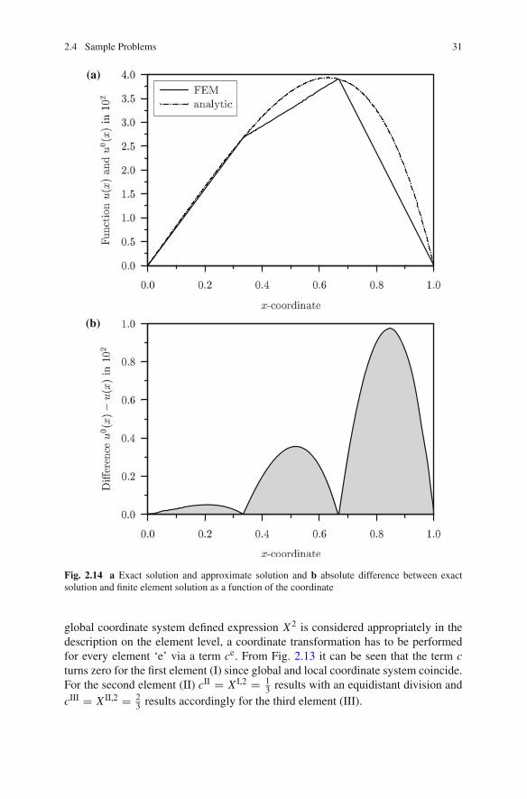
2.4 Sample Problems 31
(a)
(b)
Fig. 2.14 a Exact solution and approximate solution and b absolute difference between exactsolution and finite element solution as a function of the coordinate
global coordinate system defined expression X2 is considered appropriately in thedescription on the element level, a coordinate transformation has to be performedfor every element ‘e’ via a term ce. From Fig. 2.13 it can be seen that the term cturns zero for the first element (I) since global and local coordinate system coincide.For the second element (II) cII = X I,2 = 1
3 results with an equidistant division andcIII = X II,2 = 2
3 results accordingly for the third element (III).

32 2 Motivation for the Finite Element Method
Since the weak formulation contains the natural boundary conditions—for this seethe boundary expression in Eq. (2.89)—it can be demanded in the following that theapproach for u(x) has to fulfill the essential boundary conditions only. According tothe Galerkin method it is demanded for the derivation of the principal finite elementequation that the same shape functions for the approximate and weighting functionare chosen. Within the framework of the finite element method the nodal values uk
are chosen for the free parameters αk and the shape functions ϕk(x) are referred to asform or shape functions Nk(x). For linear shape functions the following illustrationsresult for the approximate solution and the weighting function:
u(x) = N1(x)u1 + N2(x)u2 , (2.90)
W (x) = δu1 N1(x)+ δu2 N2(x) . (2.91)
For the chosen linear shape functions, an element-wise linear course of theapproximate function and a difference between the exact solution and the approx-imate approach as shown in Fig. 2.14 are obtained. It is obvious that the error isminimal on the nodes, at the best identical with the exact solution.
References
1. Betten J (2001) Kontinuumsmechanik: Elastisches und inelastisches Verhalten isotroper undanisotroper Stoffe. Springer-Verlag, Berlin
2. Betten J (2004) Finite Elemente für Ingenieure 1: Grundlagen. Matrixmethoden, ElastischesKontinuum, Springer-Verlag, Berlin
3. Betten J (2004) Finite Elemente für Ingenieure 2: Variationsrechnung, Energiemethoden.Näherungsverfahren, Nichtlinearitäten, Numerische Integrationen, Springer-Verlag, Berlin
4. Brebbia CA, Telles JCF, Wrobel LC (1984) Boundary Element Techniques: Theory and Ap-plications. Springer-Verlag, Berlin
5. Gross D, Hauger W, Schröder J, Wall WA (2009) Technische Mechanik 2: Elastostatik.Springer-Verlag, Berlin
6. Gross D, Hauger W, Schröder J, Werner EA (2008) Hydromechanik. Elemente der HöherenMechanik, Numerische Methoden, Springer-Verlag, Berlin
7. Klein B (2000) FEM. Grundlagen und Anwendungen der Finite-Elemente-Methode, Vieweg-Verlag, Wiesbaden
8. Kuhn G, Winter W (1993) Skriptum Festigkeitslehre Universität Erlangen-Nürnberg.9. Kwon YW, Bang H (2000) The Finite Element Method Using MATLAB. CRC Press, Boca
Raton10. Oden JT, Reddy JN (1976) Variational methods in theoretical mechanics. Springer-Verlag,
Berlin11. Steinbuch R (1998) Finite Elemente - Ein Einstieg. Springer-Verlag, Berlin12. Szabó I (1996) Geschichte der mechanischen Prinzipien und ihrer wichtigsten Anwendungen.
Birkhäuser Verlag, Basel13. Zienkiewicz OC, Taylor RL (2000) The Finite Element Method Volume 1: The Basis.
Butterworth-Heinemann, Oxford