FINITE ELEMENT SOLUTIONS OF TWO-DIMENSIONAL CONTACT ...blogs.uakron.edu/cmg/files/2015/11/Finite-element-solutions-of-two... · FINITE ELEMENT SOLUTIONS OF TWO-DIMENSIONAL CONTACT

Computers & Svucrvrrs Vol. 27. No. 4. PP. 4E-466. 1987 0045.7949187 13.00 + 0.00 Printed in Great Britain. Pcrgamon Journals Ltd.

FINITE ELEMENT SOLUTIONS OF TWO-DIMENSIONAL CONTACT PROBLEMS BASED ON A CONSISTENT

MIXED FORMULATION

T. Y. CHANG, A. F. SALEEB and S. C. SHYU

Department of Civil Engineering, University of Akron, Akron, OH 44325, U.S.A.

(Received 6 February 1987)

Abstract-A consistent mixed finite element method for solving two-dimensional contact problems is presented. Derivations of stiffness equations for contact elements are made from a perturbed Lagrangian variational principle. For a contact element, both the displacement and pressure fields are independently assumed. In order to achieve a consisent formulation, thus avoiding any numerical instability, the pressure function is assumed in such a way that all non-contact modes in deformations must be excluded. Stiffness equations for four-noded and six-noded contact elements are given. Four numerical examples are included lo demonstrate the methodology.

1. INTRODUCTION Conditions involving contact between two deform- able solids, or between a solid and another medium, constitute an important class of problems in engineering applications. For example, contact of a standing or rolling pneumatic tire with the ground, design of mechanical components such as gears and bearings, and modeling of interfacial effect in metal extrusions, etc. are typical problems of practical interest. The object of a contact analysis is to determine the contact area and pressure distribution at the interface between two bodies. This class of problems is generally known to be strongly non-linear, and hence difficult to analyze since the contact areas are not known a priori and they are changing in size and shape as the load is being applied.

In the early years, the analysis of stresses and deformations developed during the contact of two or more elastic bodies was obtained via the classical elasticity method (l-31. Solutions of such problems are restricted to bodies of simple geometries, e.g. cylinders or spheres. With the advent of finite element method, the ability to obtain engineering solutions for contact problems has obviously been widened. Using constant strain elements, some frictionless contact problems based on the potential energy the- orem were solved by an indirect approach [4] in which the contact conditions were treated as subsidiary equations. Extension of this method to contact problems with friction was given in [5l in that an irreversible stick-slip process was modeled. Application of a similar technique to study the effects of clearance, load and friction on turbine blade fastenings can be found in [6,7J. An incremental solution procedure for solving contact problems with various friction conditions was presented in [8]. Another noteworthy approach is the formulation of flexibility matrices for elements along the contact boundary [91.

Although the finite element method can be applied to solving contact problems in many different ways, three major approaches may be identified on the basis of variational formulations. These are: (i) Lagrange multiplier method; (ii) penalty method; and (iii) mixed (or hybrid) method. These three approaches, though different in concept, are closely related. Some discussions on the merits and drawbacks of these approaches are given as follows.

In the Lagrange multiplier method, the constrained conditions for a contact problem are satisfied by introducing Lagrange parameters in the variational statement [IO-151. In this approach, both the nodal displacements and Lagrange parameters are treated as indpendent variables. Applications of the Lagrange multiplier method are many. For example, a numerical procedure to study the impact-contact process of axisymmetric elastic bodies with geometric non- linearity was given in [l 11. Extension of the method to the contact analysis of thin elastic shells was shown in [12]. A solution procedure for the analysis of planar and axisymmetric contact problems was presented in [13], in which the total potential of the contact forces was included in the variational equation to enforce the contact condition. A two-level contact algorithm was employed in [14], wherein a linear solution was obtained first, then the nonlinear solution was found by a Newton iteration procedure. In [l5], the Lagrange multiplier method was applied to elastodynamic contact problems with friction. In all the above work, through the use of Lagrange multipliers, corresponding contact elements can be derived in a rather straightforward manner. One major drawback of this approach, however, is that the size of the resulting system of equations will increase due to the use of independent Lagrange variables. Moreover, the associated stiffness matrix is indefinite and contains zero diagonal terms which

455

require special handling procedure in the solution of lincdr equations.

In the penalty method, the contact pressure is assumed to be proportional to the amount of pene- trations by introducing a pointwise penalty parameter. With this assumption, one can obtain the final stiffness equations which do not contain additional variables as the Lagrange multiplcr method. Penalty formulation of contact problems with Coulomb’s friction was previously introduced in [ 16) in the form of variational inequalities. Mathematical formulation of the penalty method for contact problems, discus- sion of existence and uniqueness of solutions, when Coulomb friction law is utilized, also have been given, e.g. in [l7-211. Numerical applications of this method can be found in [22-251. Note, however, that in the penalty method, the contact presssure is assumed to be proportional to the point-wise pene- trations. That is, the approximating functions for the pressure in a contact element are of the same order as the displacement functions. This in turn may lead to violation of the well-known local Babuska-Breui stability condition [26]. Hence, the corresponding pressure distribution in the contact region will generally be oscillatory. In order to control such a numerical instability phenomenon, a reduced integration scheme must be utilized[27-291. Aside from the aforementioned inconsistency, one drawback of this method is that the accuracy of the approximate solution depends strongly on the penalty number employed.

As an alternative, a mixed (or hybrid) finite element method may be employed for solving contact problems. Application of this method to contact problems is not new. For instance, a two-dimensional contact element was given in (301, in which both the displacement and stress fields were independently approximated. In (31,321, a hybrid contact element was derived from a modified complementary energy principle by introducing the continuity on the contact surface as a constraint condition and treating the contact forces as additional field variables. More recently, a mixed method based on a perturbed Lagrangian formulation was presented in [33], in which piece-wise constant pressure was assumed for a linear displacement contact element. However, pressure distributions for a more general class of elements was not mentioned. It is also noted that the key to the success of a mixed finite element formulation for contact analysis is the appropriate choice of pressure functions in conjuction with the assumed displacement polynomials. Unfortunately, no guidelines can be found in the literature for making such a choice.

In this paper, a consistent mixed formulation of two-dimensional contact elements is presented. The formulation is based on a perturbed Lagrangian variational principle in which both the displacement and pressure functions in a contact element are independently assumed. In our approximations, the displacements are assumed to be C-continuous

whereas the pressure is C-‘-continuous. By imposing

the stationarity condition of the potential functional with respect to the presssure parameters, it is possible to eliminate the pressure variables on the element level. Hence, the resulting element stiffness equations involve only the nodal displacements as ‘global’ unknowns. More importantly, specific guidelines are given on the proper choice of pressure distributions so that both numerical instability and element over- constrained response can be avoided. For the sake of clarity, this paper is limited to frictionless contact of linearly elastic bodies with small deformations. Extension of the present work to a more general class of problems, e.g. by including the effects of frictions and large deformations, should be apparent. Four numerical examples are included to illustrate the application of the proposed mixed elements.

2. FINITE ELEMENT FORMlJLATlONS

This paper is limited to frictionless contact of elastic bodies with small deformations. For the solution of nonlinear finite element equations, the con- ventional incremental loading procedure is employed.

In this section, the kinematic relations to describe two bodies in contact and an incremental form of the variational equation are given. Additionally, the finite element equations for derivation of mixed contact elements are briefly outlined.

2.1. Kinematics

Consider two bodies, designated as A and B (shown in Fig. l), each of which occupies a domain

Fig. I. Contact of two bodies.

V’ at a time [ = 0, where r +i; A, B, with a boundary s’. For a time increment [I, I + Ar], the displacement fields are denoted by a’ = u’(x’), where x’c V’. When bodies A and B are brought into contact, let S, be the unknown contact surface, which satisfies the ~lations~ip S, = VAtl Vs and S’=S:+S:+S,, where S: denotes part of the boundary with prescribed surface tractions, and S;, part of the boundary with prescribed displacements. Also, let A be a surface normal vector at XL,$, which points outward with respect to body B; T” and TB are the traction vectors at a point on S: in reference to body A and body B, respectively. At the beginning of a time increment, an initial gap g, at x6.9, in the direction of II is defined as

go=(xA--xB)*n, (1)

where x’, r I A or B, represents the ‘updated’ current coordinates of a point at time 1.

Corresponding to an increment of loading, a new gap g can be calculated and two possible contact conditions may occur: (i) gap opening

g = (Au - AuB)*n+g,>O; (2)

(ii) progressive contact

g = (Au - Au’3.n +gD=O;

Finite element so&ions of two~imensional contact problems 457

and

u = stress vector 1, J: Lagrangian multiplier, which has the phys-

ical meaning of contact surface pressure a = a ~~urbation parameter to ‘regularize’ the

classical Lagrangian formulation A() = increment of the quantity in question.

For the two bodies in equilibrium at any instant within a time interval ff, I + Ail, it is necessary to require the functional An to be stationary, i.e.

SAn = 0. (6)

If one carries out the above variational procedure, the following constraint (or contact) condition, in addition to the usual Euler equations and boundary conditions, can be recovered:

AL (Au”-Au”).n+g,,=y. (7)

g designates the current vaiue of tbe gap between bodies A and B in the direction n.

It is seen that eqn (7) represents a ‘weak’ contact condition due to the presence of a. If a+cc, the ‘exact’ contact condition of eqn (3) is recovered. Another interpretation of eqn (7) may be given as follows: it represents the constitutive equation in the normal direction of the contact surface of the two bodies. Therefore, this equation can be used to define the contact pressure A&.

2.2. A variarlona~ principle

Different forms of variational equation with the inclusion of constraint conditions can be written for two bodies in contact. For the development of mixed contact element, a perturbed Lagrangian formulation ‘is adopted [26,33]. Referring to a rectangular Cartesian system xi, i = 1,2, and 3, the incremental form of a functional An consists of the potential energy terms of bodies A and B, and terms associated with the contact ~nditions

Based on eqn (4), one may proceed with the derivation of contact elements by approximating both the displacements and contact pressure. Before proceeding further, some comments regarding continuity requirements on the basis functions of the assumed ~spia~rnen~ and contact pressure are given. The displacements Au, the same as in the usual displacement method, are Co-continuous. However, the pressure field is assumed to be C-‘-continuous. By making this assumption, the pressure parameters can be eliminated at the element level. Hence, the resulting stiffness equations for a contact element involve only the nodal displacements.

Ax = Ax(Au’, AL, ) We consider the relative normal displacement given in eqns (3) and (4):

where Ati’ is the ‘regular’ incremental potential for body A or B, i.e.

Au,, = (AuA -Aue).n=B;Aq, (8)

where B, is a transformation matrix between the element displacements and incremental nodal displacements Aq referring to the global coordinates. The incremental pressure of a contact element is approximated by

Af’ = J (u’+Aa’)~Ac’du yr

A&=P+@, (91

where P is a pressure interpolation matrix, the elements of which are polynomials of local coordinates along the contact boundary.

(l++AT’)~Atfdr (5)

0 6 5 h

Fig. 2. Two-dimensional contact elements.

Substituting eqns (8) and (9) into (4) and invoking the stationarity condition with respect to /?, one obtains

l=xH-‘(GAq+GO), (10)

where

H= PTPds (11)

G= PTB, ds (12)

and g, denotes a transformation matrix for the initial gap at a point inside the contact element in terms of the corresponding nodal values.

Substituting eqn (10) into eqn (4) and applying the stationarity condition again with respect to Aq, one obtains the familiar element stiffness equations

(k,+ak)Aq=AQ, (14)

where

Ir,=kA+kB (15)

k,=G’H-‘G (16)

AQ = AQA + AQ’ + AQ, (17)

AQ, = l..,BTd.s -aCTHe’Co. (18)

In the above, kA and k’ denote the ‘non-contact’ element stiffness matrices of bodies A and E, respectively, AQ” and AQ” are the corresponding load vectors, and AQ, a vector resulting from contact.

3. CONTACT ELEMENTS

With the general finite element equations given in the preceeding section, it remains to derive the expressions for a specific contact element. In the present paper, only two-dimensional contact elements, i.e. four-node and six-node elements as shown in Fig. 2, are considered. For derivation of the contact stiffness k,, the displacement field follows the ‘usual’ isoparametric assumption. However, special care must be given to the assumption of contact pressure in an element and some general remarks are made below.

3. I. General considerations

It is important to note that the key to the successful development of a mixed contact element lies in the appropriate assumption of pressure function, i.e. entries of the P matrix in eqn (9). At one extreme, for instance, an over-use of polynomial terms for A& will give a mixed element which is no better than a penalty model. On the other hand, an under-use of polynomial terms will result in poor numerical results. Therefore a balance on the choice of pressure terms in conjunction with the assumed displacement field is necessary.

To make a proper choice of the pressure function, two considerations must be given: (i) all zero energy modes must be suppressed; and (ii) the contact element must have a favorable constraint index in order to avoid any ‘locking’ problem. Each of these two points are discussed in this section. Detailed

Finite element solutions of two-dimensional contact problems 459

discussions of these and related items, in the context of other constrained-media applications (e.g. plates and shells), can be found in [34].

Suppression of zero energy modes is perhaps the most important requirement in the formulation of a mixed finite element (or in making multi-field assumptions). In fact, many of the recent mathematical studies on the numerical stability and convergence requirements of the multi-field methods have shown the delicate behavior of such methods [26,35-371. In particular, a general requirement known as the local Babuska-Brezzi (LBB) conditions (see e.g. [26]) must be satisfied for a mixed finite element in order to guarantee its numerical stability and convergence. In the same spirit, a procedure was proposed by Pian and Chen [38] to suppress kinematic deformations for a hybrid/mixed element. Based on the consideration of deformation energy, they suggested that while the total number of stress terms must be greater than or equal to the number of deformation modes represented by the element, at least one stress term corresponds to the strain terms derived from the strain-displacement relations. Although this procedure was intended for the formulation of a ‘structural’ element, the concept, with some modification, is also applicable to a contact element.

Since the contact stiffness matrix k, which appeared in eqn (14) is obtained from the contact potential I, A1, .g d.r of eqn (4), it is appropriate to examine the order of relative normal displacement Au, along the contact boundary S,. For a four-node contact element, Au, has the expression

Au,=a,+~~r, (19)

Contact hIodes

where r denotes the local coordinate along the contact boundary. Based on the procedure given in [38], it appears that the pressure function should also be a linear function of r. If the pressure is so assumed, numerical instability in the calculation of pressure distributions will occur. If one examines eqn (19) more closely, it can be considered as two distinct types of deformation modes: (1) a uniform deformation<ontact mode; and (2) a linear deformation- non-contact mode (shown in Fig. 3(a)). The pressure term must correspond only to the contact mode, i.e. a constant-term pressure assumption is sufficient in this case:

Hence,

AI, = j3,. (20)

(21)

In the case of a six-node element, the relative displacement is

Au, = II, + u2r + u3rz. (22)

The above equation again can be looked upon as representing constant- and linear-contact modes as well as a quadratic non-contact mode (Fig. 3(b)). Obviously, the appropriate choice of the corresponding pressure function would then be

That is,

Al, = j?, + /$r. (23)

P= (1 r). (24)

Non-Contact Modes

(a) 4-Node Contact Element

A ,/4-

S==u “* .\’

(b) 6-Node Contact Element

Fig. 3. Contact and non-contact modes for two-dimensional contact element.

c AS DC-B

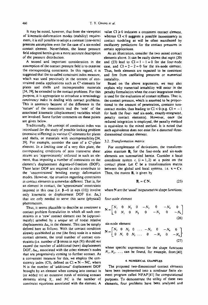
460 T. Y. CHANG el al.

It may be noted, however, that from the viewpoint of kinematic-deformation modes (stability) requirement, it is still possible to adopt a constant (one-term) pressure assumption even for the case of a six-noded contact element. Nevertheless, the linear pressure field adopted herein gives a more accurate description of the pressure distribution.

A second and important consideration in the assumption of the contact pressure field is to examine the corresponding constraints. In this regard, it is suggested that the so-called constraint index measure, which was used previously in the context of constrained media applications such as C-elements for plates and shells and incompressible materials 134,391. be extended to the contact problems. For this purpose, it is appropriate to introduce a terminology consisfency index in dealing with contact problems. This is necessary because of the difference in the ‘nature’ of the constraints and the ‘role’ of the associated kinematic (displacement) variables which are involved. Some further comments on these points are given below.

Traditionally, the concept of constraint index was introduced for the study of possible locking problem (excessive stiffening) in various C-elements for plates and shells, or materials with incompressibility 134, 391. For example, consider the case of a C-plate element. In a limiting case of a very thin plate, the corresponding conditions of zero transverse shear strains arc ‘approximately’ enforced in such an element, thus imposing a number of constraints on the element’s displacement degrees-of-freedom (DOF). These latter DOF are required to also contribute to the ‘unconstrained’ bending energy deformation modes. However, the situation regarding constraints in contact elements is somewhat different. That is, for an element in contact, the ‘approximate’ constraints imposed in this case (i.e. g-0 in eqn (10)) involve only kinematic or displacement DOF (i.e. Au,) that are only needed to serve this same (physical) phenomenon.

Thus, it seems plausible to describe as consisrenr a contact problem formulation in which all such constraints in a ‘new’ contact element can be (approximately) satisfied by a unique set of nodal relative displacements Au, in the element. This can be simply defined here as follows. With the contact condition already established at one (the first) node in a mixed contact element, the total number of contact constraints (i.e. number of B-terms in eqn (9)) should not exceed the number of additional (new) displacement DOF, AU,, associated with the other element’s nodes that are progressively coming to further contact. As a convenient measure for this, we employ the consistency index (Cl), defined as Cl = N -NC, where N is the number of ‘addiGonal’ displacement DOF brought by an element when coming into contact in (or added to) an extensive mesh of existing contact elements along S,, and NC is the number of constraint equations associated with the element. A

value CI 2 0 indicates a consistent contact element, whereas CI < 0 suggests a possible inconsistency in contact modeling as will be often manifested by oscillatory predictions for the contact pressures in certain applications.

As an illustration, consider the two mixed contact elements above. It can be easily shown that eqns (20) and (23) lead to CI = I - 1 = 0 for the four-node case, and CI = 2- 2 = 0 for the six-node element. Thus, both elements are expected to be consistent and free from oscillating pressures or numerical instability.

Based on the above arguments, we may also explain why numerical instability will occur in the penalty formulation when the exact integration order is used for the evaluation of contact stiffness. That is, the contact pressure, which is assumed to be proportional to the amount of penetration, contains non- contact modes, thus leading to CI < 0 (e.g. CI = - 1 for both the four- and six-node, exactly-integrated, penalty contact elements). However, once the reduced integration is employed, the penalty method is equivalent to the mixed method. It is noted that such equivalence does not exist for a distorted three- dimensional contact element.

3.2. Transformafion matrix

For completeness of derivations, the transformation matrices B, for the four-node and six-node elements are summarized herein. Consider a local coordinate system r, (i = 1.2) at a point on the contact plane. Let C be a transformation matrix between the global and local systems, i.e. x = Cr. Then, the matrix B, is given by

B,=CN, (25)

where N are the ‘usual’ isoparametric shape functions:

four-node element

N= [

N, 0 N, 0 -N, 0 -N, 0

0 N, 0 N, 0 -N, 0 -N, 1 (26) six-node element

N_ N,

-[

0 N1 0 . . . -N, 0 -N6 0

0 N, 0 N2 .., 0 -N5 0 1 -N6 ’

(27)

where specific expressions for the shape functions N,rNz,.... can be found, for example, from [do].

4. NUMERICAL EXAMPLES

The proposed two-dimensional contact elements have been implemented into a nonlinear finite element program called NFAP [41] for computational purposes. To demonstrate the utility of these two elements, four problems have been analyzed and


P=27Or: lb

(3 r=4 in.

Fig. 4. Finite element mesh of a Hertz contact problem.

numerical results are compared with those obtained from other sources. Since the scope of the present paper is limited to the solution method of contact problems with small deformations, only node-to- node contact is considered. Undoubtedly, this limitation must be removed when the effect of large deformation is to be included.

4.1. Hertzian contacl problem

This problem has frequently been cited as a bench- mark due to the availability of analytical solution. A long solid cylinder resting on a rigid base is subjected to a uniform line load along its axis (Fig. 4). No friction is considered for this problem.

After several trial runs on various mesh sixes, a model, consisting of 25 eight-node plane strain elements for the cylinder and six-node contact elements shown in Fig. 4, appears to be a reasonable mesh for the intended analysis. The material property of

0.000.200.400.600.601.001.201.40l.60!.60

CONTACT LENGTH (B) IN.

Fig. 5. Contact pressure distribution at various extents of contact.

the cylinder is assumed to be linearly elastic and isotropic and the constants are:

Young’s modulus: E = 3.0 x IO’ksi Poisson’s ratio: 0 = 0.0

Perturbation parameter: a = 3.0 x IO*.

Finite element results are plotted in conjunction with those of analytical solution [I] in Figs 5 and 6. The calculated nodal displacements are of the order of IO-’ times the radius of the cylinder; that is, small deformation prevails. The corresponding contact region is about 15% of the cylinder diameter. In Fig. 5, pressure distributions vs different contact areas are shown with the Hertz solution. It is Seen that excellent agreement is obtained. In Fig. 6 the progressive load vs contact areas is plotted. Again,

1.60

0.000.200.400.600.601.001.201.401.600

CONTACT LENGTH (Bl IN.

Fig. 6. Contact force vs contact area.

I I I I I I t I

q ICI HIXED HETHOD - HERTZ SOLUTION

.is

462 T. Y. CHaNG et al.

p=5 lb

I

E = 3.0 x 104psi

v = 0.0

Fig. 7. Contact between two beams. mesh subdivision,

good agreement between the finite element result and

analytical solution can be seen. Identical results were obtained when the number of elements were doubled from that of six-noded elements. Moreover, different values were assumed for a in the analysis. It was found that when a varies between IO* and 3 x lo*, no significant change in numerical results was observed.

4.2. Contact between two beams

The second example is the contact of two short beams with slightly curved surfaces shown in Fig. 7 and this problem was previously considered in [9]. Each beam was modeled by 24 eight-noded plane stress elements and 18 six-noded contact elements were considered at the interface. In addition to the mixed method, the penalty method with two vari- ations was also empIoyed for comparison: (i) exact integration order; and (ii) reduced integration. Two equal concentrated forces, opposite in direction, were applied to the beam system to produce a maximum contact area which is 3.3% of the beam length.

In the analysis, a fairly large perturbation number a = 3.0 x IO9 was used.

In Fig. 8 the pressure vs contact area plots for the mixed method, penalty method and (analytical) Hertz solution are shown. It is seen that the results obtained from the mixed method and penalty method with reduced integration agree quite well with the analytical solution, Some numerical oscillation is apparent when the penalty method with exact integration order is employed.

4.3. indentation of two ehstic blocks

Two elastic blocks of the same material were super- imposed on top of each other. A concentrated force P was applied at the center of the upper (smaller) block. Dimensions of the set-up and elastic constants are illustrated in Fig. 9. Using symmetry, only one- half of the system was modeled by 41 eight-noded elements as shown in Fig. IO. The interface between the two blocks was represented by five elements. Initially, the two-block system was assumed to be


= 0.60

0 0

$&_ 0.10 0

0 _ 0.20 I-

2 0.00

0.00 1.00 2.00 3.00 4.00 5.00 6.bO

(X/RI *IO_’

Fig. 8. Contact pressure distribution between two beams.

already in contact. As the load is being increased, some detachment near the outside comers will occur. A total load of P = 1960 N was applied to the

P-1960N

1

I /++ 70 cm ,-j

E = 9.31 x 10’ kpa

u = 0.3

Fig. 9. Two contact blocks subjected to a point load.

Fig. IO. Finite element idealization.

Ccl tflXED tlETHOD - REFERENCE SOLUT 1 ON cl51

4*00

3.00

E t s 2.00

~ r

0.00 .I1 0.00 0.50 1.00 l-50 2.00 2.50

CONTACT LENGTH WI) *IO

Fig. i 1. Variation of normal contact pressure along the contact surface.

system in five equal increments to reach solution convergence. In the analysis, a fairly large value of a(9.6 x IO”) was chosen, although the solution is generally insensitive to the magnitude of e. The same problem was previously analyzed by using the flexibility matrix method [42]. Corresponding to the maximum load f,, , the normalized contact pressure (P/P,, P, = average pressure) along the interface is shown in Fig. 11. Also, the analysis results indicate that two contact elements near the outside corner of the interface become detached. That is, the contact zone is extended only to three contact elements from the center line of the two-block system. As indicated in Fig. I 1, excellent correlation between the mixed method and the reference solution given in[lS] is obtained.

4.4. A rubber disk

Considered herein was a rubber disk encased in its inner wall with a steel cylinder as shown in Fig 12(a). The disk rested on a smooth, rigid platten and two concentrated forces were imposed on the cylinder as indicated in the figure. Since the cylinder was bonded together with the rubber disk by high-strength epoxy, no relative motion between the rubber disk and cylinder was allowed during the course of deformations. The geometry of the disk-cylinder assembly is shown in Fig. 12(b). Since the focus of this analysis was to determine the contact behavior of the rubber disk in comparison with the test data given in [43], the SBR rubber was treated as linearly elastic: E = 220 psi, u = 0.45.

Due to the fact that the steel is relatively rigid compared to the modulus of rubber, only the inclusion part of the cylinder was considered for contact analysis. Correspondingly, the applied load was transferred to the center of the disk. Roth the steel inclusion and rubber disk are modeled by six- noded elements as shown in Fig. 13. The total load,

464 T. Y. GANG et al.

E (rubber) : 220 psi

Y (rubber) = 0.45

E(slrrl) - 3 rlo’psl

“(steel) =o.o

Ri = 2.717”

RO z 5”

Fig. 12. Contact loading of a rubber disk.

with a magnitude of 160 lb, was imposed onto the disk in 15 increments, and 3-5 iterations were needed to reach solution convergence for each load step. In Fig. 14 the pressure distribution in the contact region obtained by (i) mixed method and (ii) penalty method with exact integration order is shown. The solid line represents the experimental measurements. The results obtained by the mixed method, although they show general agreement with the experimental data, deviate from the measured maximum response by about 5%. Considerable oscillation is indicated from the results calculated from the penalty method in

connection with a high Poisson ratio used for this problem.

The load vs hub displacement (vertical displacement at the center of the disk) is shown in Fig. IS. The numerical results follow the same trend as the experimental measurements, but show a stiffer response. A possible explanation is that nonlinear material response of the rubber may have contributed to the discrepancy.

5. CONCLUSION

On the basis of a perturbed Lagrangian variational principle, two contact elements, i.e. four-noded and six-noded elements, were formulated by a mixed method. In this method. both the relative displace-

Fig. 13. Rubber disk problem: 2/D finite element mesh.

I .oo

0.40 4 I

0.00 0.20 0.40 0.60 0.80

DISTANCE FROM CENTER (IN.)

Fig. 14. Measured pressures from center to one end of footprint of the SBR rubber disk.


1.80

1.60

“0 - I.40 .

1.20

between cylindrical shafts and sleeves. /no. 1. Engng &i. 5, 541-554 (1967).

4. E. A. Wilson and B. Parsons, Finite element analysis of elastic contact problems using differential displacements Inr. J. Nwner. Meth. Engng 2, 384-395 (1970).

5. S. Ohte, Finite element analysis of elastic contact problems. Bull. JSME 16, 797-804 (1973).

6. C. H. Chan and 1. S. Tuba. A finite element method for

2 1.00

d 0.80

9 2 0.60

i &

0.40

I- 0.20

contact problems of solid bodies: 1. Theory and valida- lion. Inr. J. Mech. Sci. 13, 615625 (1971).

7. C. H. Chan and I. S. Tuba. A finite element method for contact problems of solid bodies-application to turbine blade fastenings. Irrf. 1. Mech. Sci. 13, 627639 (1971).

8. N. Okamoto and M. Nakaxawa, Finite element incremental contact anllysis with various frictional conditions. Inf. J. Numer. Meth. Engng 14, 337-357 (1979).

9. A. Francavilla and 0. C. Zienkiewicz. A note on numerical computation of elastic contact problems.

0.00 Int. J. Numer. Merh. Ehgng 9, 913-924 (1975).

0.10 0.20 0.30 0.40 IO. T. J. R. Hughes, R. L. Taylor, J. L. Sackman, A.

HUB DISPLACEMENT (IN.) Cumier and W. Kanoknukulchai, A finite element method for a class of contact-impact problems. Com-

Fig. IS. Computed and measured load-displacement responses of the rubber disk.

pur. Merh. appl. Mech. Engng 0, 249-276 (1976). T. J. R. Huahes. R. L. Tavlor and W. Kanoknukulchai. II. A finite ele;ent method ior large displacement contact and impact problems. Formulation in finite element analysis. In US-German Symposium on Finite Elemenr Method (Edited by Bathe, Oden and Wunderlich) (1978). E. Stein and P. Wriggcrs, Calculation of impact contact problems of thin elastic shells taking into account geometrical nonlinearities within the contact re8ion. Compur. Merh. appl. Mcch. Engng 34, 861-880 (1982). K. J. Bathe and A. Chaudhary. A solution method for planar and axisymmetric contact problems. fnr. J. Numer. Merh. Engng 21, 65-88 (1985). P. Wriggers and B. Nour-Omid, A two-level iteration method for solution of contact problems. Compur. Merh. appl. Mech. Engng 54, 131-144 (1986). Wen-Hwa Chen and Pwu Tsai, Finite element analysis of elastodynamic sliding contact problems with friction. Compur. Strucl. 22, 925-938 (1986). G. Duvaut and J. L. Lions, Inequalities in Mechanics and Physics. Springer, Berlin (1976). N. Kikuchi and Y. J. Song, Penalty/finite element approximations of a class of unilateral problems in linear elasticity. Quart. appl. Math. 39, l-22 (1981). L. T. Campos, J. T. Oden and N. Kikuchi. A numerical analysis of a class of contact problems with friction in elaatostatics. Cornput. Merh. appl. Mech. Engng 34, 821845 (1982). J. T. O&n and N. Kikuchi, Finite element methods for constrained problems in elasticity. In;. 1. Numer. Merh. figng 18, 701-725 (1982). E. B. Pires and J. T. Gden. Analysis of contact problems with friction under oscillating loads. Compur. Merh. appl. Mech. Engng 39, 337-362 (1983). _ J. T. Dden and E. B. Pires. Alnorithms and numerical results for finite element approximations of contact problems with non-classical friction laws. Compur. Sfrucl. 19, 137-147 (1984).

L. Ascione and A. Grimaldi. Penalty formulations of the unilateral contact problem between plates and an elastic half spaa. Dipartimento di Strutture, Universita

ments and contact pressure in an element are independently assumed. The unique feature of the present work is that the pressure function is approximated in such a way that all non-contact modes of deformations must be suppressed. Such a contact fotmu- lation is termed consistent here, and a convenient measure for it, the consistency index, is suggested to investigate the success or otherwise of various contact elements. For both contact elements proposed in the paper, a favorable value CI >, 0 was obtained.

By doing this, the so-called LBB condition is satisfied and hence no numerical instability can appear in the calculation of contact pressure.

In summary, the present formulation offers the following advantages:

(I) Finite element equations for a contact element are consistently derived without introducing any ad hoc assumptions.

(2) No numerical instability appears in the contact pressure distribution.

(3) It gives fairly accurate contact pressure pre- diction.

(4) The element is relatively insensitive to geo-

metric distortion as compared to its displacement counterpart.

Our future objective is to extend the present method to solutions of contact problems with friction effects. Moreover, formulation of three-dimensional contact elements is also underway.

12.

13.

14.

15.

16.

17.

18.

19,

20.

21.

22.

REFERENCES della CaIabria Cosenza, Italy. 23. J. 0. Hallquist. G. L. Goudreau and D. J. Benson,

S. Timoshenko and J. N. Goodier, Theory of Eiasricity. Sliding interfaas with contact-impact in large-scale McGraw-Hill, New York (1951). Lagrangian computations. Compur. Merh. appl Mech. C. J. Hooke, Numerical solution of axisymmetric-stress Engng 51, 107-137 (1985). problems by point matching. J. Strain Anal. 5. 25-37 24. G. Yagawa and H. Hirayama, A finite element method (1970). for contact problems related to fracture mechanics. H. D. Conway and K. A. Famham, Contact stresses ht. 1. Numer. Meth. Engng 28, 2175-2195 (1984).

466 T. Y. CHANG el a/.

25

26

27.

28.

29.

30.

31.

32.

33.

34.

N. Kikuchi, A smoothing technique for reduced inte-

P. Wriggers. J. C. Simo and R. L. Taylor. Penalty and augmented Lagrangian formulations for contact prob-

gration penalty methods in contact problems. Inr. J.

lems. In Proceedings NUMETA Conference. Swansea

Numer. Merh. Engnng 18, 343-350 (1982).

(1985).

J. Txng and M. D. Olson, The mixed finite element

G. F. Carey and 1. T. Dden, Finire Elemenrs: A Second Course. II. Prentice-Hall, Englewood Cliffs, NH (1983).

method applied to two-dimensional elastic contact

J. T. Oden, N. Kikuchi and Y. J. Song. Reduced

problems. Inr. J. Numer. Meth. Engng 17, 99-1014

integration and exterior penalty methods for finite

(1981).

element approximations of contact problems in incompressible elasticity. TJCOM Report 80-2. Univ. Texas at Austin, Austin, TX (1980). Y. J. Song, J. T. Oden and N. Kikuchi. RlP-methods for contact problems in incompressible elasticity. TICOM Report N&7, Univ. Texas at Austin, Austin. TX (1980).

35. H. Stolarski and T. Belytschko, Limitation principles for mixed finite elements based on the Hu-Washizu variational formulation. In Hybrid and Mixed Finite Elcmenr Me/hods (Edited by R. L. Spilker and K. W. Reed). Appl. Mech. Diti. ASME 73, 123-132 (1985).

36. 1. Babuska. J. T. Oden. and J. K. Lee. Mixed hybrid finite element approximations of second-order elliptic boundary-value problems, part II. Campuf. Merh. appl. Mech. Engng 14, l-22 (1978).

38.

39.

37. W. M. Xue and S. N. Atluri. Existence and stability, and discrete BB and rank conditions. for general mixed- hybrid finite elements in elasticity. In Hybrid and Mixed

Fini/e Element Merhodc (Edited by R. L. Spilker and R. K. Reed). Appl. hitch. Dir.. ASME 73, 91-112 (1985). T. H. H. Pian and D. P. Chen, On the suppression of zero energy deformation modes. Inr. J. Numer. Merh. Engng 19, 1741-1752 (1983). D. S. Malkus and T. J. R. Hughes. Mixed finite element methods-reduced and selective integration techniques: a unified concept. Compur. Merh. appl. Mech. Engng 12. 63-81 (1978). R. D. Cook, Concepts and Applications of Fmire Elemenl

Analysis, 2nd Edn. John Wiley. New York (1981). T. Y. Chang, NFAP-a general purpose nonlinear finite element program. Department of Civil Engineering. University of Akron, October I, 1978 (revised on January IS. 1987). T. D. Sachdeva and C. V. Ramakrishnan. A finite element solution for the two-dimensional elastic contact problems with friction. Inf. 1. Numer. Merh. Engng 17. 1257-1271 (1981). R. A. Ridha. K. Satyamurthy. L. R. Hirschfelt and R. E. Holle. Contact loading of a rubber disk. Paper presented at the First Meeting of the Tire Society, University of Akron, Akron, OH. 25-26 March, 1982.

K. Kubomura and T. H. H. Pian, Solutions of contact 40. problems by the assumed stress hybrid model, Research in Nonlinear Structural Solid Mechanics, NASA Conf. 41. Pub. 2147, pp. 21 l-224 (1980). T. H. H. Pian and K. Kubomura. Formulation of contact problems by assumed stress hybrid elements. In Nonlinear Finire Element Analysis in Swucrural 42. Mechanics (Edited by W. Wunderlich er a!.). Springer, Berlin (1981). J. C. Simo. P. Wriggers and R. L. Taylor, A perturbed Lagrangian formulation for the finite element solution 43. of contact problems. Compur. Meth. appl. Mech. Engng SO, 163-180 (1985). A. F. Saleeb, T. Y. Chang, and W. Graf. A quadri- lateral shell element using a mixed formulation. Compur. Sfrucf. (to appear).

Documents

FINITE ELEMENT SOLUTIONS OF TWO-DIMENSIONAL CONTACT ...blogs.uakron.edu/cmg/files/2015/11/Finite-element-solutions-of-two... · FINITE ELEMENT SOLUTIONS OF TWO-DIMENSIONAL CONTACT