TREATMENT OF OILFIELD PRODUCED WATER WITH DISSOLVED AIR FLOTATION

by

Kehinde Temitope Jaji

Submitted in partial fulfilment of the requirements for the degree of Master of Applied Science

at

Dalhousie UniversityHalifax, Nova Scotia

August 2012

© Copyright by Kehinde Temitope Jaji, 2012

ii

DALHOUSIE UNIVERSITY

DEPARTMENT OF CIVIL AND RESOURCE ENGINEERING

The undersigned hereby certify that they have read and recommend to the Faculty of

Graduate Studies for acceptance a thesis entitled “Treatment of Oilfield Produced Water

with Dissolved Air Flotation” by Kehinde Temitope Jaji in partial fulfilment of the

requirements for the degree of Master of Applied Science.

Dated: August 8, 2012

Supervisor: Dr. Magaret Walsh

Co-supervisor: Dr. Craig Lake

Readers: Dr. Jennie Rand

Dr. Graham Gagnon

iii

DALHOUSIE UNIVERSITY

DATE: August 8, 2012

AUTHOR: Kehinde Temitope Jaji

TITLE: Treatment of Oil Field Produced Water with Dissolved Air Flotation

DEPARTMENT OR SCHOOL: Department of Civil and Resource Engineering

DEGREE: MASc CONVOCATION: October YEAR: 2012

Permission is herewith granted to Dalhousie University to circulate and to have copied for non-commercial purposes, at its discretion, the above title upon the request of individuals or institutions. I understand that my thesis will be electronically available to the public.

The author reserves other publication rights, and neither the thesis nor extensive extracts from it may be printed or otherwise reproduced without the author’s written permission.

The author attests that permission has been obtained for the use of any copyrighted material appearing in the thesis (other than the brief excerpts requiring only proper acknowledgement in scholarly writing), and that all such use is clearly acknowledged.

Signature of Author

iv

I will like to dedicate this thesis to my mother, Mrs. Olabisi Bolanle Jaji, for all her sacrifices, love and support through the years.

v

Table of ContentsList of Tables ................................................................................................................... viii

List of Figures .....................................................................................................................ix

Abstract ...............................................................................................................................xi

List of Abbreviations and Symbols Used ......................................................................... xii

Acknowledgements...........................................................................................................xiv

Chapter 1: Introduction ........................................................................................................1

1.1 Objectives...................................................................................................................3

1.2 Thesis Organization....................................................................................................3

1.3 Originality of Research ..............................................................................................4

Chapter 2: Literature Review...............................................................................................6

2.1 Produced Water ..........................................................................................................6

2.1.1 Dispersed Oil .......................................................................................................7

2.1.2 Oil in Water Emulsions .......................................................................................8

2.1.3 Dissolved Oil Concentrations ..............................................................................9

2.2 Treatment of Produced Water ..................................................................................11

2.2.1 Flotation - Dissolved Air Flotation (DAF) ........................................................12

2.2.2 Removing Dissolved Oil from Produced Water................................................13

2.3 Pre-treatment Techniques for DAF ..........................................................................14

2.3.1 Coagulation........................................................................................................14

2.3.2 Adsorption .........................................................................................................16

Chapter 3: Materials and Methods.....................................................................................24

3.1 Synthetic Produced Water ........................................................................................24

3.2 Liquid – Liquid Extraction Methodology ................................................................24

3.3 Dissolved Air Flotation (DAF) Unit ........................................................................25

3.3.1 Operation of the DAF Unit ................................................................................26

3.4 Analytical Methods ..................................................................................................27

Chapter 4. Evaluation of Oil and Grease Measurement Using Infrared and Ultraviolet Spectrometric Methods. .....................................................................................................29

4.1 Introduction .............................................................................................................29

4.2 Materials and Methods .............................................................................................33

vi

4.2.1 Synthetic Produced Water .................................................................................33

4.2.3 Fourier Transform Infrared (FTIR) Method......................................................34

4.2.4 UV-Vis Spectrometry Method...........................................................................34

4.3 Results and Discussion.............................................................................................37

4.3.1 Standard Oil & Grease Curves with FTIR Spectrometry ..................................37

4.3.2 Standard Oil & Grease Curves with UV-Vis Spectrometry ..............................39

4.3.3 UV Spectra for Synthetic Produced Water Standards .......................................42

4.4 Conclusions ..............................................................................................................45

Chapter 5: Evaluation of Coagulation and Adsorption Pre-Treatment Processes .............46

5.1 Introduction ..............................................................................................................46

5.2 Materials and Methods .............................................................................................48

5.2.1 Coagulant/Adsorbents .......................................................................................48

5.2.2 Experimental Design .........................................................................................49

5.3 Analytical Methods ..................................................................................................55

5.4 Results and Discussion.............................................................................................55

5.4.1. Control Experiments.........................................................................................55

5.4.2 Coagulation/DAF Experiments .........................................................................56

5.4.3 PAC/DAF Experiments .....................................................................................61

5.4.4. Organoclay and DAF Experiments...................................................................67

5.4.5 Treatment Process Comparison .........................................................................73

5.5 Conclusions ..............................................................................................................75

Chapter 6: Removal of Dissolved Oil Components with Adsorption-DAF Process .........76

6.1 Introduction ..............................................................................................................76

6.2 Materials and Methods .............................................................................................77

6.2.1 Materials ............................................................................................................77

6.2.2 Benzene/Methanol Stock solution .....................................................................78

6.2.3 Benzene Removal Experiments.........................................................................83

6.3 Results ......................................................................................................................85

6.4 Conclusion................................................................................................................88

Chapter 7: Conclusions ......................................................................................................89

7.1 Conclusions ..............................................................................................................89

vii

7.2 Recommendations ....................................................................................................91

References..........................................................................................................................92

Appendices.......................................................................................................................101

Figure A-1: UV Absorption Spectra for Crude Oil in Hexane Standards....................101

Figure A-2: UV Absorption Spectra for Crude Oil in Petroleum ether Standards.......101

Table B-1: Data, Oil & Grease Removal from Synthetic Produced Water..................102

Table B-2: Data, Turbidity Removal from Synthetic Produced Water........................103

viii

List of Tables

Table 2.1: Chemical Composition of Produced Water from Main Sources in the Norwegian Sector of the North Sea (1999 – 2000) 6

Table 2.2: Oil and Grease Removal Technologies Based on Size of Removable Particles (Argonne National Library) 12

Table 2.3: Oil and Grease Reduction by Organoclay and GAC 23

Table 2.4: Benzene Reduction by Organoclay and GAC 23

Table 3.1: DAF Operating Parameters 26

Table 4.1: Preparation of Calibration Standards for FTIR Analysis. 34

Table 4.2: Preparation of Calibration Standards for UV-Vis Spectrophotometric Analysis. 35

Table 4.3: Preparation of Synthetic Produced Water Calibration Standards for UV-Vis Analysis using Petroleum Ether as Solvent. 36

Table 4.4: Peak Wavelength and R2 value for the Solvents; Dichloromethane, Hexane and Petroleum ether. 41

Table 4.5: Summary of UV-Vis and FTIR Analysis of Synthetic Produced Water Samples. 44

Table 5.1: Factorial Design 50

Table 5.2: pH Adjustment during PAC-DAF Experiments 52

Table 5.3: Concentration of Surfactant from Organoclay that Dissolved in Produced Water 53

Table 6.1: Concentration of 0.6 mg/L Benzene Standards Measured by GC-FID 80

Table 6.2: Measured concentration of MDL samples 83Table 6.3: Optimum Coagulant and Adsorbent Pre-treatment Conditions for DAF process 84

ix

List of Figures

Figure 1.1: Offshore Produced Water discharge (Source: Argonne National Library) 2

Figure 2.1: Process of Coagulation, Flocculation and Flotation 15

Figure 3.1: Bench scale DAF Unit 25

Figure 4.1: FTIR Absorption Spectra for Crude Oil in Tetrachloroethylene Standards 37

Figure 4.2: FTIR Calibration Curve at 2930cm Wavelength 38

Figure 4.3: UV-Vis Absorption Spectra for Crude Oil in Dichloromethane Standard 39

Figure 4.4: Calibration curve for Crude oil in Dichloromethane Standard at 228 nm. 40

Figure 4.5: Calibration curve for Crude oil in Hexane standard at 225 nm. 40

Figure 4.6: Calibration curve for Crude Oil in Petroleum Ether Standard at 226 nm. 41

Figure 4.7: UV Spectra for Synthetic Produced Water Standards 42

Figure 4.8: UV Calibration curve for Synthetic Produced Water Standards at 226 nm. 43

Figure 5.1: Schematic Diagram Illustrating Coagulation/DAF Treatment Scheme 51

Figure 5.2: Schematic diagram illustrating the PAC/DAF Treatment scheme 52

Figure 5.3: Schematic diagram illustrating the OC/DAF Treatment scheme 54

Figure 5.4: % Oil and Grease and % Turbidity Removal for the Control Treatment 56

Figure 5.5: Effect of pH on OG Removal by FeCl3/DAF Treatment 57

Figure 5.6: Effect of pH on Turbidity Removal 58

Figure 5.7: Effect of coagulant dose on OG Removal by FeCl3/DAF treatment 59

Figure 5.8: Effect of Coagulant dose on Turbidity Removal 60

x

Figure 5.9: Effect of pH on OG Removal by PAC/DAF treatment 61

Figure 5.10: Effect of pH on Turbidity Removal by PAC/DAF Treatment 63

Figure 5.11: Effect of Mixing Time on OG Removal by PAC/DAF Treatment 63

Figure 5.12: Effect of Mixing Time on Turbidity Removal by PAC/DAF Treatment 64

Figure 5.13: Effect of PAC dose on OG Removal by PAC/DAF treatment 65

Figure 5.14: Effect of PAC dose on Turbidity Removal by PAC/DAF Treatment 66

Figure 5.15: Effect of pH on OG Removal by OC/DAF Treatment 68

Figure 5.16: Effect of pH on Turbidity Removal by OC/DAF Treatment 68

Figure 5.17: Effect of Mixing Time on OC/DAF Treatment 69

Figure5.18: Effect of Mixing Time on Turbidity Removal by OC/DAF Treatment 70

Figure 5.19: Effect of OC dose on OG Removal by OC/DAF treatment 71

Figure 5.20: Effect of OC dose on Turbidity Removal by OC/DAF Treatment 72

Figure 5.21: Oil and Grease Removal with Alternative Treatment Regimes 73

Figure 5.22: Turbidity Removal with Alternative Treatment Technologies 74

Figure 6.1: % Benzene Removal After Treatment 85

xi

Abstract

Produced water is one of the major by products of oil and gas exploitation which is produced in large amounts up to 80% of the waste stream. Oil and grease concentration in produced water is the key parameter that is used for compliance monitoring, because it is easy to measure. For Canadian offshore operations, the current standard is a 30-day volume weighted average oil-in-water concentration in discharged produced water not exceeding 30 mg/L. Treatment of produced water may therefore be required in order to meet pre-disposal regulatory limits. The measurement of oil in produced water is important for both process control and reporting to regulatory authorities. Without the specification of a method, reported concentrations of oil in produced water can mean little, as there are many techniques and methods available for making this measurement, but not all are suitable in a specific application.

The first part of this study focused on selecting a suitable analytical method for oil and grease measurement in oil field produced water. Petroleum ether was found to offer a comparative dissolution of crude oil as dichloromethane and hexane; it was therefore used as the solvent of choice for the UV-Vis spectrophotometric analysis of oil and grease in synthetic produced water. Results from the UV-Vis spectrophotometric and FTIR spectrometric analytical methods were found to be comparable; it confirmed that UV-Vis spectrometry could potentially serve as an alternative method for measuring oil and grease in oil field produced water. However, while the UV-Vis method may have limitations in measuring oil and grease concentrations below 30 mg/L, the FT-IR method was found to be equally efficient at measuring both high and low oil and grease concentrations.

Dissolved air flotation (DAF) was the primary treatment technology investigated in this study for removing oil and grease from synthetic produced water. By itself, DAF achieved less than 70% oil and grease (OG) removal, and was not able to achieve a clarified effluent OG concentration of 30 mg/L required for regulatory discharge limits. At an optimum condition of 20 mg/L ferric chloride (FeCl3) at pH 8 (70.6% OG removal), coagulation was found to significantly improve the performance of the DAF unit (p < 0.05). At the optimum conditions of 100 mg/L PAC dose, pH 8 and a mixing time of 10 minutes (77.5% OG removal) and 300 mg/L OC dose, pH 8 and a mixing time of 10 minutes (78.1% OG removal), adsorption was also found to significantly improve the performance of the DAF unit (p < 0.05 in both cases). Adsorption with organoclay was recommended as the best pre-treatment for optimizing the performance of DAF in removing oil and grease from offshore oil field produced water. The bench-scale experiments showed that turbidity removal results were consistent with the OG removal results.

Without pre-treatment, DAF achieved significant removal of benzene from produced water due to the volatile nature of benzene. Therefore comparable levels of benzene removal was observed by the DAF, FeCl3/DAF, PAC/DAF and OC/DAF treatment schemes; 79.3 %, 86.6 %, 86.5 %, 83.5% respectively. Finally, as benzene is known to be carcinogenic to humans, this study recommends the incorporation auxiliary equipment in its design, for the treatment of the off-gas (VOCs, particularly BTEX) released during the removal of dissolved oil from the oil field produced water.

xii

List of Abbreviations and Symbols Used

API American Petroleum Institute

BTEX Benzene, toluene, ethylbenzene and xylene

CEC Cation exchange capacity

CH Carbon-hydrogen

EF Electro-flotation

FTIR Fourier transform infra red

GAC Granular activated carbon

GC-FID Gas chromatography-flame ionization detector

IAF Induced air flotation

IFT Interfacial tension

NPD Naphthalene, phenanthrene and dibenzothiophene

OC Organoclay

OG Oil and grease

PAC Powdered activated carbon

PAH Polycyclic aromatic hydrocarbons

QAC Qarternary amine cation

TMAC Tetramethyl ammonium chloride

xiii

TPH Total petroleum hydrocarbon

UV-Vis Ultraviolet-visible light

VOCs Volatile organic compounds

xiv

Acknowledgements

First of all, I will like to thank the Almighty God for His divine grace, favour and

mercies upon my life. He has once again shown Himself faithful in my life.

I will also like to appreciate my supervisor, Dr. Margaret Walsh; her outstanding

leadership, wealth of knowledge, wisdom and sincere interest in the success of her

students were key factors in my successful completion of this project. Dr. Craig Lake, my

co-supervisor was also a huge support base for me, always willing to offer important

advice and to take critical steps that made my project easier to accomplish. My gratitude

also goes out to Petroleum Research Atlantic Canada (PRAC) for making the funds

available for this project to be completed.

I cannot express enough appreciation to Heather Daurie, Shelley Oderkirk, Jessica

Younker and all of my friends and colleagues who have shown me support in so many

different ways. Thank you all.

I will particularly like to acknowledge the special person in my life, Laura Joy

Sarah Payne. You have literarily walked this journey with me, holding my hands through

the high and the low moments. You have been a huge support base for me emotionally,

spiritually and intellectually. I am very grateful to God for making you and your family a

part of my life.

Finally, I will like to appreciate my family who have shown such understanding

and support for me. Important family events were sacrificed as a result of this project but

through it all our bond of love and family remained a huge pillar of strength for me.

1

Chapter 1: Introduction

Water produced during oil and gas extraction operations constitutes the industry’s most

important waste stream on the basis of volume. By volume, water production represents

approximately 98 % of the non-energy related fluids produced from oil and gas operations,

yielding approximately 14 billion barrels of water annually (Veil et. al, 2004). Across the United

States, when compared to the annual oil (1.9 billion barrels), (Arthur et. al, 2005) and gas (23.9

trillion cubic feet), (Arthur et. al, 2005) production, the argument could be made that the oil and

gas produced would be more appropriately identified as a by-product to production of water.

Produced water includes formation water, injection water and process water that is

extracted along with oil and gas during petroleum production. In addition, a portion of the

chemicals added during processing of reservoir fluids may partition to the produced water

(CNSOPB, 2010). Produced water contains both soluble and insoluble (oil droplets not removed

prior to physical separation) petroleum fractions, and are found at variable concentrations. This

petroleum fraction consists of a complex mixture of organic compounds similar to those found in

crude oils and natural gases (Tellez et. al, 2005)

At most offshore production installations, produced water is separated from the

petroleum process stream and after treatment, is discharged to the marine environment or

disposed of in a subsurface formation (CNSOPB, 2010). Treatment of produced water may be

required in order to meet disposal regulatory limits or to meet beneficial use specifications (e.g

for recreational purposes, drinking water for stock and wild life etc.). If the oil and gas operator

aims to utilize a low-cost disposal option such as discharge to surface waters, the produced water

must meet or exceed limits set by regulators for key parameters (Arthur et. al., 2005).

2

Figure 1.1: Offshore Produced Water discharge (Source: Argonne National Library)

Oil and grease concentration in produced water is the key parameter that is used for

compliance monitoring for marine discharge effluent quality. Regulatory standards for overboard

disposal of produced water into offshore surface waters vary from country to country. Current

regulations require the “total oil and grease” content of the produced water to be reduced to

levels ranging from 15 to 50 mg/L depending upon the host country (Arnold and Stewart, 2008).

For Canadian offshore operations, the current standard is a 30-day volume weighted average oil-

in-water concentration in discharged produced water not exceeding 30 mg/L (CNSOPB, 2010),

in the United States, it is 29 mg/L (U.S Department of Energy). Produced water toxicity is

regulated only in the United States where government permit is necessary to limit the toxicity of

produced water discharged into the waters (Arnold and Stewart, 2008).

The measurement of oil in produced water is important for both process control and

reporting to regulatory authorities. Oil in produced water is a method-dependent parameter, a

point which cannot be emphasised enough. Without the specification of a method, reported

3

concentrations of oil in produced water can mean little, as there are many techniques and

methods available for making this measurement, but not all are suitable in a specific application

(Yang et. al, 2006).

1.1 Objectives

The main hypothesis of this research was that the performance of a dissolved air flotation

(DAF) unit in treating offshore produced water can be optimised through pre-treatment with

either coagulation or adsorption processes. This hypothesis was tested using the following

objectives:

Evaluate appropriate analytical methods for measuring oil and grease in produced water.

Evaluate the impact of coagulant (ferric chloride) and adsorbents (powdered activated

carbon (PAC) and organoclay (OC)) pre-treatment processes on DAF treatment efficacy for

the removal of dispersed oil from produced water

Evaluate the impact of coagulant (Ferric chloride) or adsorbent (PAC or OC) pre-treatment

on DAF for the removal of dissolved oil from produced water

1.2 Thesis Organization

Following this introduction, Chapter 2 gives a detailed literature review of the available

pre-treatment and treatment technologies available for oil and gas produced water. It also

introduces produced water, its characterization as well as the key water quality component of

produced water that is regulated. Chapter 3 describes the materials, methods and equipment that

were used for the preparation and treatment of synthetic produced water in the laboratory. It also

describes the same for the analytical methods that were used to measure the water quality

characteristics of the synthetic produced water used in this study. Chapter 4 discusses the results

for the solvents that were compared in order to select an appropriate solvent to be used for UV-

4

Vis spectrophotometric analytical method. It also discusses the results for the comparison of the

UV-Vis analytical method and the FTIR spectrometric analytical method for oil and grease

measurement. Chapter 5 presents and discusses the results of pre-treatment of produced water

with coagulation and adsorption before DAF for the removal of dispersed oil. Chapter 6

discusses the results for the removal of the dissolved oil using the optimized operating conditions

of coagulation and adsorption determined in Chapter 5. Chapter 7 summarizes the conclusions of

the study and presents recommendations for future research.

1.3 Originality of Research

Several studies have been conducted in which coagulation has been used to optimize

DAF for the treatment of produced water (Al-Shamrani et. al, 2002; Zouboulis and Avranas,

2000). Hami et al (2007) found that powdered activated carbon was able to optimize DAF in

removing biochemical oxygen demand (BOD) and chemical oxygen demand (COD) from

refinery waste water. However, there appears to be a shortage or lack of information about the

use of adsorption for the optimization of DAF in removing oil and grease from produced water.

Therefore, this study aimed to fill this research gap by evaluating the effect of two adsorbents;

powdered activated carbon (PAC) and organoclay (OC) on the performance of DAF in removing

oil and grease from produced water. This research will particularly provide new information

about the use of organoclay as an adsorbent in a continuous stirred tank reactor (CSTR) design in

contrast to conventional adsorption column designs that may be used to optimize DAF in

removing both dispersed and dissolved oil from produced water. There is well documented

success of the use of organoclay in removing dispersed and dissolved oil from produced water

and oil – water emulsions (Alther, 1995; Doyle and Brown, 2000; Man Chi-Lo et al, 1996),

however it has been difficult to find any record of its use in optimizing DAF for the same

5

purpose. Also, organoclay used in this research was in the powdered form which is different

from the packed form (with larger grain sizes) in which it has been used in previous studies.

Finally, it is very important to define the analytical method used for oil and grease

measurement. Also important is the choice of solvent to be used for the selected analytical

method. Hexane and dichloromethane are two solvents that have been used for the UV

spectrophotometric analysis of oil and grease. However, the use of hexane has been subjected to

control because it is highly flammable and dichloromethane is considered to be potentially

carcinogenic to humans. This research aimed to evaluate the performance of petroleum ether, a

solvent that is not considered to be carcinogenic and not as flammable as hexane, as an

alternative solvent that could be used for the UV-Vis spectrophotometric analysis of oil and

grease in produced water. This is because although petroleum ether is identified to be one of the

solvents that can be used for UV-Vis spectrophotometric analysis, there is little or no record of

its use for this purpose.

6

Chapter 2: Literature Review

2.1 Produced Water

Produced water is one of the major by-products of oil and gas exploitation that is

produced in large amounts up to 80% of the waste stream (McCormack et al., 2001). Depending

on geological conditions and field position, produced water may have complex composition

including: organic or inorganic ingredients like: salts, metals, dispersed oils, phenols, organic

acids, dissolved hydrocarbons like: benzene, toluene, ethylbenzene and xylene (BTEX), poly

aromatic hydrocarbons (PAHs) like: naphthalene, phenanthrene and dibenzothiophene (NPD)

and their C1-C3 alkyl homologues and also some compounds which may be added to it during

oil separation process (Utvik, 1999).

In Table 2.1 the chemical composition of produced water from the main discharges in the

Norwegian Sector is summarised for both oil and gas condensate platforms (Utvik et. al, 2002).

Table 2.1: Chemical Composition of Produced Water from Main Sources in the Norwegian Sector of the North Sea (1999 – 2000) (Source Utvik et.al, 2002)

Compound group Unit Low HighDispersed oil mg/L 10.0 40.0BTEX mg/L 1.0 40.0NPD mg/L 0.9 10.0PAH mg/L 0.01 0.13Organic acids mg/L 55.0 760.0Phenol mg/L 0.1 6.0C1 – C4 alkylated phenols mg/L 0.17 11.3C4 – C7 alkylated phenols mg/L 0.1 0.8Radioactive elements Bq/L 0.1 10.0

BTEX: Benzene, Toluene, Ethylbenzene, Xylene NPD: Naphthalene, Phenanthrene, Dibenzothiophene, including their C1 – C3 alkyl homologues PAH: Polycyclic aromatic hydrocarbons represented by 16 EPA PAH, except naphthalene and phenanthrene

Table 2.1 shows that among the dissolved oil components of produced water, the organic

acids have the highest concentration followed by the compounds of the BTEX group. Dispersed

oil is also present in large amounts in produced water.

7

Oil and grease concentration in produced water is the key parameter that is used for

compliance monitoring, because it is easy to measure (Arnold and Stewart, 2008). Total oil and

grease is defined as the combination of both the dispersed and dissolved liquid hydrocarbons and

other organic compounds contained in produced water. This term is referenced in certain

regulatory standards and is commonly used to evaluate treatment system design. Total oil and

grease consists of normal paraffinic, asphaltic and aromatic hydrocarbon compounds plus

specialty compounds from treatment chemicals. The measurement of total oil and grease is

dependent on the analysis method used (Arnold and Stewart, 2008).

2.1.1 Dispersed Oil

Produced water contains hydrocarbons in the form of dispersed oil droplets, which, under

proper conditions, can be coalesced into a continuous hydrocarbon liquid phase and then

separated from the aqueous phase using various separation devices (Arnold and Stewart, 2008).

The amount of dispersed oil in a produced water stream will vary depending on the influence of

several factors, including the density of the oil, the shear history [upstream processing and pipe

fittings, control valves, pumps, and other equipment that create turbulence and shearing action]

of the droplet (Arnold and Stewart, 2008) and the interfacial tension (IFT) between the water and

the oil (Stephenson, 1992). The diameters of these oil droplets can range from over 200 microns

to less than 0.5 microns and may be surrounded by a film (emulsifier) that impedes coalescence.

The relative distribution of droplet sizes is an important design parameter and is influenced in

addition to the above mentioned factors by temperature, down hole operating conditions and

presence of trace chemical contaminants.

If the oil density is not significantly different from the water density, there is little driving

force to move the droplet to the surface for coalescence and collection. If the oil has been

8

through many shear devices at high velocity or pressure, the droplets entering the water-

treatment system will be far smaller than they could have been. As a droplet moves through

chokes, valves, pumps, or other constrictions in the flow path, the droplet can be torn into

smaller droplets by the pressure differential across the devise. Small droplets can be stabilized by

low IFT between the oil and the produced water. This situation often is caused by improper use

of production chemicals. The addition of any surfactant to an oil/water system reduces the IFT

between the oil and water. Thus, the addition of excess production chemicals will reduce the IFT

to such low levels that coalescence and separation are extremely difficult (Stephenson, 1992).

2.1.2 Oil in Water Emulsions

Most emulsions encountered in the oil field are water droplets in an oil continuous phase

and are called “normal emulsions.”(Arnold and Stewart, 2008). The water is dispersed in the

form of very small droplets ranging between 100 to 400 microns in diameter. Oil droplets in a

water continuous phase are known as “reverse emulsions” and can occur in produced water

treatment operations. If the emulsion is unstable, the oil droplets will coalesce when they come

in contact with each other and form larger droplets, thus breaking the emulsion. An unstable

emulsion of this type will break within minutes. A stable emulsion is a suspension of two

immiscible liquids in the presence of a stabilizer or emulsifying agent that acts to maintain an

interfacial film between the phases (Schramn, 1992). Chemicals, heat, settling time, and

electrostatics are used to alter and remove the film and cause emulsion breakdown. Untreated

stable emulsions can remain for days or even weeks. Emulsion breakers for water-in-oil

emulsions, also known as destabilizers or demulsifiers, are oil-soluble and are added to the total

well stream ahead of the process equipment. Being oil-soluble, the emulsion breaker is carried

9

with the crude. Thus, if the emulsion is not broken in the first-stage separator, the chemical has

additional time to act in the subsequent separators and the stock tank.

Oil-in-water emulsions can be broken by “reverse emulsion breakers,” which are special

destabilizers or demulsifiers. These are similar to the conventional emulsion breakers except that

they are water-soluble. Reverse emulsion breakers are generally injected into the water stream

after the first oil–water separation vessel. Typical concentrations are in the 5 to 15 ppm range,

and over treating should be avoided because these chemicals can stabilize an emulsion (Schramn,

1992). The emulsions in produced water will become oil in the form of dispersed droplets after

the emulsion film is broken. The droplets will coalesce to yield an oily film that can be separated

from the produced water using gravity settling devices such as skim vessels, coalescers, and plate

separators. However, small droplets require excessive gravity settling time, so flotation cells or

acceleration enhanced methods such as hydrocyclones and centrifuges are used. Equipment

selection is based on the inlet oil’s droplet diameter and concentration (Arnold and Stewart,

2008).

2.1.3 Dissolved Oil Concentrations

Dissolved oil is also called “soluble oil,” representing all hydrocarbons and other organic

compounds that have some solubility in produced water. The source of the produced water

affects the quantity of the dissolved oil present. Produced water derived from gas/condensate

production typically exhibits higher levels of dissolved oil. In addition, process water condensed

from glycol regeneration vapour recovery systems contains aromatics including benzene,

toluene, ethyl benzene, and xylenes (BTEX) that are partially soluble in produced water (Arnold

and Stewart, 2008).

10

In a particular oil and gas field, the waters in the producing strata may contain dissolved

non-hydrocarbons (i.e. “organic acids”) which have been generated locally, have been brought in

by moving water or have been extracted from oil in the reservoir. In general gas accumulations

are not expected to contain significant amounts of these so called organic acids in the gas phase

(Place, 1991).

The amount and nature of soluble oil or non-hydrocarbon organic materials that may be

in the produced-water stream also depends on the variability of the soluble oil with the type of

oil, i.e. whether the oil is of the paraffinic, asphalthenic, or gas condensate type. The chemical

characteristics of the soluble oil compounds generally place them in the following classes:

aliphatic hydrocarbons, phenols, acids, and aromatic compounds. Dissolved hydrocarbons

(decane through tetratriacontane) have been determined to be present in produced water in the

ranges of 606 to 2677 g/L (Caudle and Stephenson, 1988). Phenols have been found in varying

amounts in the water associated with all three oil types; however, produce water from gas

condensate operations tend to have higher quantities of phenols and low-molecular weight

aromatic compounds (Callaghan and Baumgartner, 1990). Water produced with paraffinic oils

often has high concentrations of simple fatty acids, while water produced with asphaltenic oils

contain notable amounts of naphthenic acids. After Somerville et al (1987) found quantities of

acetic acid in North Sea produced water near 700 mg/L, it was realized that earlier results

indicating that there was only a small quantity of low-molecular weight fatty-acid compounds

present in the extract was because of the lack of solubility of the low molecular weight fatty

acids in Freon [which was the fluid used to extract dissolved oil from acidified produced water]

(Stephenson, 1992).

11

The solubility of crude oil in produced water has not been extensively documented, but

the solubility of several hydrocarbons can illustrate the potential range. Field experience

indicates that solubility does not change appreciably with the temperatures used during water

treatment, specifically from 77 to 167 0F (25 to 75 0C) (Arnold and Stewart, 2008). Solubility

does increase significantly, however, as temperatures rise above 167 0F (75 0C) (Arnold and

Stewart, 2008). The effect of high salinity on reducing the solubility of dissolved hydrocarbons

implies that produced water from gas well and gas processing sources should be mixed with the

saltiest brine available to reduce the dissolved oil concentration (Arnold and Stewart, 2008). The

dissolved hydrocarbons would be forced out of solution from the water into the vapour phase or

into a dispersed oil droplet removed by gravity separation equipment.

Water chemistry and hydrocarbon solubility are also related to toxicity. Dissolved

saturated paraffinic (aliphatic) petroleum hydrocarbons have low solubilities in water and have

not demonstrated toxicity. Aromatics, such as benzene, toluene, ethyl benzene, and xylene, are

more soluble and more toxic (Arnold and Stewart, 2008).

2.2 Treatment of Produced Water

Current oil and grease removal treatments include: API gravity separators. corrugated

plate separators, hydrocyclones, mesh coalescers, media filters, centrifuges, membrane filters

and flotation. Gravity separation is ineffective with small oil droplets or emulsified oil. To

improve performance therefore, retention time is drastically increased as oil droplet sizes

decrease. API gravity separators are limited to removing oil droplet sizes down to 150 microns

while corrugated plate separators can remove oil droplet sizes down to 40 microns. However,

flotation is known to remove oil droplet sizes down to 3-5 microns especially when chemicals

12

are added (Arthur D.J et al., 2005). Table 3 summarises the oil and grease removal technologies

currently in use based on the size of the removable particles.

Table 2.2: Oil and Grease Removal Technologies Based on Size of Removable Particles (Source: Veil et. al)

Oil Removal Technology Minimum size of particles removed (microns)

API gravity separator 150Corrugated plate separator 40Induced gas flotation (no flocculant) 25Induced gas flotation (with flocculants) 3-5Hydrocyclone 10-15Mesh coalesce 5Media filter 5Centrifuge 2Membrane filter 0.01

2.2.1 Flotation - Dissolved Air Flotation (DAF)

Several studies have been conducted on the use of flotation as a wastewater treatment

technique; in their review, Rubio et al (2002) suggested that there are currently three

conventional flotation techniques: electro-flotation (EF), Induced (dispersed) air flotation (IAF)

and dissolved air flotation (DAF). IAF and DAF have been used extensively in the removal of

stable oil emulsions (Strickland, 1980; Bennett, 1988; Belhateche, 1995). IAF utilizes bubbles

between 40 to 1000 m in size, turbulent hydrodynamic conditions and the process has low

retention times; normally < 5 minutes. DAF on the other hand employs micro bubbles 30-100

m in size and quiescent regimes, however, because retention times are higher (20 to 60

minutes), it is inefficient when treating high volume effluents and high flow rates (Rubio et al,

2001).

The presence of emulsified oil in water, droplets around 50 m in size causes problems in

phase separation by conventional techniques. The flotation separation of very fine oil droplets (2

13

to 30 m) is even more complicated and usually requires fine bubbles, quiescent hydrodynamic

conditions in the cell separation zone or emulsion breakers prior to flotation (Gopalratman et al.,

1988). This therefore suggests that the micro bubbles and the quiescent regimes employed by

DAF make it the best technique for separation of very fine oil droplets. Pre-treatment of the

emulsified oil in water using coagulation/flocculation or adsorption are methods that can be used

to effect emulsion breaking prior to flotation in order to optimize the performance of DAF.

DAF is an effective method for removing low density particles from suspension and for

clarifying low turbidity, highly coloured waters where light flocs are produced (Gregory and

Zabel, 1990; Al-Shamrani et. al, 2002; Hami et al, 2007). The micro bubbles are generated by a

reduction in pressure of water pre-saturated with air at pressures higher than atmospheric; the

supersaturated water is forced through needle valves or nozzles and clouds of bubbles, 30-100

m in diameter are produced just downstream of the constriction (Bratby and Marais, 1977;

Lazaridis et al., 1992).

2.2.2 Removing Dissolved Oil from Produced Water

Gravitational-type separation equipment will not remove dissolved oil. Thus, a high level

of total oil and grease could be discharged if the produced water source contains significant

quantities of dissolved oil. Produced water streams containing high concentrations of dissolved

oil can be recycled to a fuel separator to help reduce the quantity of dissolved oil in the water

effluent. Other technologies, such as bio-treatment, adsorption, solvent extraction and

membranes are currently being evaluated by industry for removing dissolved oil, but such

processes are not yet readily available for commercial applications. However three processes

have been proven to remove these components from water: bio-treating, adsorption using

activated charcoal and acidification [organic acids only] (Place, 1991).

14

It is essential that actual water test analysis data for dissolved and dispersed oil

concentrations are needed in the planning stage prior to designing a water treatment facility for a

specific application. If the design engineer assumes a value for the dissolved oil content without

first having obtained actual water test analysis for the specific produced water stream to be

treated, the facility design may not be capable of treating the effluent water to meet regulatory

compliance specifications. Therefore, lab testing is required first (Arnold and Stewart, 2008).

2.3 Pre-treatment Techniques for DAF

Pre-treatment of emulsified oil in water can be done by using coagulation or adsorption to

impart emulsion breaking prior to flotation in order to optimize the performance of DAF.

2.3.1 Coagulation

Coagulation is the addition of chemicals and the provision of mixing so that particles and

some dissolved contaminants are aggregated into larger particles that can be removed by solids

removal processes such as sedimentation, dissolved air flotation, rapid filtration or membrane

filtration (Dempsey, 2006). Figure 2.1 illustrates the process of coagulation, flocculation and

flotation.

15

Figure 2.1: Process of Coagulation, Flocculation and Flotation

Over the usual range of natural water pH (e.g., 5 to 9) particles nearly always carry a

negative surface charge. Because of their surface charge, aquatic particles are often colloidally

stable and resistant to aggregation. For this reason, coagulants are needed to destabilize the

particles (Duan and Gregory, 2003)

The primary mechanisms responsible for effective coagulation have been identified to be

charge neutralization and sweep flocculation with both dependant on pH and the coagulant dose

(Dempsey, 2006; Duan and Gregory, 2003). Four zones of coagulant dosage have been defined

at which these mechanisms are observed (Duan and Gregory, 2003):

Very low coagulant dosage; particles still negative and hence stable;

Dosage sufficient to give charge neutralization and hence coagulation

Higher dosage giving charge neutralization and restabilization

Still higher dosage giving hydroxide precipitate and sweep flocculation.

Coagulants that are widely used in water and wastewater treatment include hydrolysing metal

salts that are based on aluminium and iron; aluminium sulfate and ferric chloride are the most

16

commonly used inorganic coagulants (Dempsey, 2006; Duan and Gregory, 2003). Typical

reactions of aluminium and iron salts in water are shown in the Equations 2.1 and 2.2 below:

Equation 2.1

Equation 2.2

These salts consume alkalinity as can be seen in the release of hydrogen ions into the

solution. This may require the addition of alkaline agents as pH of coagulation is critical. Ferric

salts work best in a pH range of 4.5 to 5.5; where more positively charged species are present

and the negative charge on colloids is less (Pernitsky, 2003), whereas aluminum salts are most

effective around a pH range of 5.5 to 6.3 (Droste, 1997).

According to Packham et al. (1965), ferric salts are less sensitive to pH because ferric

hydroxide is much less soluble than aluminium hydroxide; hence ferric hydroxide is precipitated

over a much broader pH range. This means that Fe-based coagulants can be used over a much

greater pH range than Al-based coagulants without worrying about dissolved metals

concentrations in the finished water (Pernitsky, 2003). It was also found that Fe(III) coagulants

can produce better turbidity and colour removal than Al(III) coagulants (Morris and Knocke,

1984; Knocke et al, 1986) and that, at both low and high temperatures (5 oC and 20 oC

respectively), Fe(III) coagulants produced stronger floc than Al(III) coagulants (Hanson and

Cleasby, 1990)

2.3.2 Adsorption

Although adsorption has been used as a physical-chemical process for many years, it is

only over the last four decades that the process has developed to a stage where it is now

17

a major industrial separation technique for the oil and gas industry (Richardson et al, 2002). In

adsorption, molecules distribute themselves between two phases, one of which is a solid whilst

the other may be a liquid or a gas.

Adsorption occurs when molecules diffusing in the fluid phase are held for a period of

time by forces emanating from an adjacent surface. The surface represents a gross discontinuity

in the structure of the solid, and atoms at the surface have a residue of molecular forces which

are not satisfied by surrounding atoms such as those in the body of the structure. These residual

or van der Waals forces are common to all surfaces and the only reason why certain solids are

designated “adsorbents” is that they can be manufactured in a highly porous form, giving rise to

a large internal surface. In comparison the external surface makes only a modest contribution to

the total, even when the solid is finely divided.

The adsorption which results from the influence of van der Waals forces is essentially

physical in nature. Because the forces are not strong, the adsorption may be easily reversed. In

some systems, additional forces bind absorbed molecules to the solid surface. These are chemical

in nature involving the exchange or sharing of electrons, or possibly molecules forming atoms or

radicals. In such cases the term chemisorption is used to describe the phenomenon. This is less

easily reversed than physical adsorption, and regeneration may be a problem. Chemisorption is

restricted to just one layer of molecules on the surface, although it may be followed by additional

layers of physically adsorbed molecules.

It is often convenient to think of adsorption as occurring in three stages as the adsorbate

concentration increases (Richardson et al, 2002). Firstly, a single layer of molecules builds up

over the surface of the solid. This monolayer may be chemisorbed and associated with a change

in free energy which is characteristic of the forces which hold it. As the fluid concentration is

18

further increased, layers form by physical adsorption and the number of layers which form may

be limited by the size of the pores. Finally, for adsorption from the gas phase, capillary

condensation may occur in which capillaries become filled with condensed adsorbate, and its

partial pressure reaches a critical value relative to the size of the pore.

Adsorbents are available as irregular granules, extruded pellets and formed spheres. The size

reflects the need to pack as much surface area as possible into a given volume of bed and at the

same time minimize pressure drop for flow through the bed. Sizes of up to about 6 mm are

common. To be attractive commercially, an adsorbent should embody a number of features

(Richardson et al, 2002):

it should have a large internal surface area.

the area should be accessible through pores big enough to admit the molecules to be

adsorbed. It is a bonus if the pores are also small enough to exclude molecules which it is

desired not to adsorb.

the adsorbent should be capable of being easily regenerated.

the adsorbent should not age rapidly, that is lose its adsorptive capacity through

the adbsorbent should be mechanically strong enough to withstand the bulk handling

continual recycling and vibration that are a feature of any industrial unit.

Some adsorbents used in wastewater treatment include activated carbon and organoclay.

2.3.2.1 Activated Carbon

In some of the earliest recorded examples of adsorption, activated carbon was used as the

adsorbent. Naturally occurring carbonaceous materials such as coal, wood, coconut shells or

bones are decomposed in an inert atmosphere at a temperature of about 800 K. Because the

product will not be porous, it needs additional treatment or activation to generate a system of fine

19

pores. The carbon may be produced in the activated state by treating the raw material with

chemicals, such as zinc chloride or phosphoric acid, before carbonising (Richardson et al, 2002).

Alternatively, the carbon from the carbonising stage may be selectively oxidised at temperatures

in excess of 1000 K in atmospheres of materials such as steam or carbon dioxide. Activated

carbon has a typical surface area of 106 m2/kg mostly associated with a set of pores of about 2

nm in diameter.

Activated carbon may be used as a powder, in which form it is mixed in with the liquid to

be treated, and then removed by filtration (powdered activated carbon (PAC)). It may also be

used in granular form, referred to as granular activated carbon (GAC) packed in adsorption

columns (Gupta and Suhas, 2009). Because it has a low affinity for water, activated carbon may

preferentially adsorb components from aqueous solution or from moist gases and by carefully

choosing the starting material and the activating process, it has been possible in recent years to

generate in carbon a pore system with a narrow span of pore sizes with a mean pore diameter of

perhaps 0.6 nm. Such products are known as carbon molecular sieves (Richardson et al, 2002).

Despite the success attributed to activated carbons in the removal of organic and

inorganic substances from waste water, their use is sometimes restricted in view of higher cost

(Gupta and Suhas, 2009). Also, the activated carbons after their use become exhausted and are

no longer capable of further adsorbing the contaminants. When this happens, they have to be

regenerated for further use in treating wastewater using methods like: thermal, chemical,

oxidation and electrochemical regeneration, the most common being thermal. It is worthwhile to

note that regeneration of activated carbon also adds cost. For this reason, research has made

attempts to prepare low cost alternative adsorbents to replace activated carbons in pollution

control through adsorption process (Ali and Gupta, 2007).

20

2.3.2.2 Organoclay

Natural materials or the wastes/by-products of industries or synthetic prepared materials,

which cost less and can be used as such or after some minor treatment as adsorbents are

generally called low-cost adsorbents (LCAs). Among natural materials clays occupy a prominent

position being low cost, available in abundance and having good sorption properties. There are

various types of clays which include: ball clay, bentonite (smectite), common clay, sepiolite, fire

clay, fuller’s earth (attapulgite and montmorillonite varieties) and kaolin (Gupta and Suhas,

2009). The sorption capacities of clays can be improved even further by ion exchange with

inorganic cations or organic cations to give organoclays (Betega de Paiva et al., 2008; Gupta and

Suhas, 2009)

Among the clay minerals, bentonites (smectites) especially montmorillonite, have been

extensively used to prepare organoclays because of its excellent properties, such as high cation

exchange capacity, swelling behaviour, adsorption properties and large surface area (Betega de

Paiva et al., 2008).

Organoclay is produced by combining sodium montmorillonite clay with a cationic

quaternary amine salt, which replaces adsorbed sodium by ion exchange. Resulting clay surfaces

become organophilic. Montmorillonite is a three-layer clay mineral. It has a 2:1 configuration

consisting of two silica tetrahedral sheets with a central alumina octahedral sheet. The occasional

substitution of Al3+ for Si4+ in the tetrahedral sheets and Mg2+, Fe2+, Li2+, or Zn2+ for Al3+ in the

octahedral sheet results in a net negative surface charge on the clay. This charge imbalance is

usually equalized by the presence of Na+ and Ca2+ cations that are adsorbed between the

crystalline layers and around the edges of the platelets. The total amount of these cations is

21

called the cation exchange capacity (CEC) and it is expressed in terms of milliequivalents per

100 g of dry clay.

The ability of sodium montmorillonite, also known as smectite or bentonite, to undergo

cation exchange is well documented. Drillers are well acquainted with the effect of salt or

anhydrite (calcium ion) on fresh-water drilling muds. Exploration and production operations

have routinely used potassium chloride and ammonium chloride solutions to prevent formation

damage caused by clay migration and swelling during well completion and servicing operations

(Doyle and Brown, 2000).

The ability of cationic organic molecules to exchange on bentonite clay is also well

documented. Jordan (1949) discovered that the complex formed by montmorillonite and certain

quaternary amine salts was organophilic. While bentonite clay tends to swell in the presence of

water, the treated bentonite swelled in the presence of certain organic liquids. Tetramethyl

ammonium chloride (TMAC) and other quaternary amines have also become popular

replacements for potassium chloride in workover and completion fluids because of the high

chloride levels required for inorganic salts such as KCl to stabilize clays. These amines stabilize

formation clays.

By way of explanation, a quaternary amine cation (QAC) can be described by

substituting an organic group for each of four hydrogen atoms in ammonium (NH4+). For

example, tetramethyl ammonium is formed by substituting a methyl group for each hydrogen

atom. A QAC carries the same valence as ammonium and readily exchanges with the sodium in

montmorillonite. When large organic cations are exchanged, however, the cation exchange is

virtually irreversible because the resulting material is hydrophobic. In practical terms,

22

organoclay is unaffected by water salinity and will not yield, swell or flocculate when contacted

by formation brines (Doyle and Brown, 2000).

Hydrocarbons are removed from water by adsorption. The quaternary amines create

organic pillars” between the clay platelets that increase the interlamellar distance and facilitate

the formation of a hydrocarbon partition (Doyle and Brown, 2000). Hence organoclay

completely removes free hydrocarbons from wastewaters and also removes dissolved

hydrocarbons including benzene, toluene, ethylbenzene, and xylene (BTEX) (Man-Chi Lo et al,

1996; Sharmasarkar et al, 1999). When used in conjunction with a polishing stage of granular

activated carbon (GAC), organoclay removes free and dissolved hydrocarbons to levels well

below current water quality standards (Doyle and Brown, 2000).

Organoclay possesses several advantages over GAC for removing free hydrocarbons (Doyle

and Brown, 2000), these include:

• It offers much higher adsorption and can adsorb up to 60-70% hydrocarbon by weight.

• It is most efficient in removing insoluble and dispersed hydrocarbons that contribute to

Total Petroleum Hydrocarbon (TPH) and Oil & Grease measurements.

• It tolerates concentration spikes that result from separator or treater upsets and accidental

oil carry-over from storage tanks.

• Adsorbed hydrocarbons do not desorb. Spent media would likely be classified in the

United States as a nonhazardous waste.

In their field study, Doyle and Brown (2000) found that by itself the commercial

organoclay product, ET-1 removed oil and grease as well as total petroleum hydrocarbon (TPH)

to non-detectable levels (Table 2.3). They also found that a substantial portion of the BTEX was

removed by the organoclay with levels falling to non-detectable after adsorption by activated

23

carbon. Their field data supports predictions by Dentel et al (1994) that organoclay will be less

effective with increasing solubility of the contaminant, hence benzene exhibited the poorest

removal by the organoclay (Table 2.4).

Table 2.3: Oil and Grease Reduction by Organoclay and GAC (Source: Doyle and Brown, 2000)

Table 2.4: Benzene Reduction by Organoclay and GAC (Source: Doyle and Brown, 2000)

Benzene ConcentrationSample I.D. Influent After Organoclay After GACETV 1A mg/L 3.14 2.85 <0.50ETV2A mg/L 1.81 2.01 <0.50ETV3A mg/L 0.90 <0.50 <0.50ETV4A mg/L 0.73 <0.50 <0.50

Oil and Grease Concentration (mg/L)Sample I.D. Influent After Organoclay After GACETV 1A mg/L 151.0 <1.0 1.2ETV2A mg/L 18.0 <1.0 1.4ETV3A mg/L 7.4 <1.0 1.1ETV4A mg/L 79.0 <1.0 <1.0

24

Chapter 3: Materials and Methods

3.1 Synthetic Produced Water

Synthetic produced water stock solution was prepared by weighing 2 g of crude oil in a

blender bucket placed on a laboratory mass balance. 150 L of a surfactant, Triton X (Sigma

Aldrich) was added as well as 1 L of salt water stock solution (32 g/ L). The mixture was

blended (Oster 12 speed blender) for 5 minutes and allowed to settle for another 5 minutes after

which the uniformly mixed layer was decanted into a 1 L bottle. The salt water stock solution (32

g/L) was prepared by adding 480 g of sea salt (H2Ocean) to 15 L of Ultra-pure water which was

obtained by using a Milli-Q system from Millipore (Milford, M.A, USA).

3.2 Liquid – Liquid Extraction Methodology

The liquid – liquid extraction technique outlined in the Standard Test Method for Oil and

Grease Petroleum Hydrocarbons in Water (ASTM D3921-96, 2011) was used in this study. The

procedure was carried out as follows. All glassware was rinsed twice with approximately 100

mL Milli-Q water followed by 30mLs of the solvent. The pH of each synthetic produced water

standard solution (250 mL) was then reduced to less than 2 by adding 3mL of 6 M hydrochloric

acid solution. 30 mL of solvent was then added to the produced water standard (250 mL) in a 2 L

separatory funnel. The mixture was vigorously shaken for 2 minutes and left to settle for 10

minutes. Depending on the density of the solvent used, the extract laden solvent either floated on

or settled below the water line. The layers were separated by draining the water (or solvent

phase) from the bottom of the funnel. In order to dehydrate the extract of entrained water, it was

filtered through 10 g of anhydrous granular sodium sulphate (Na2SO4) after which it was

collected, stored and sealed in a 100 mL standard volumetric cylinder.

25

This procedure was repeated two more times on the produced water solution that

remained. The extract that was collected from each step was added to the one from the previous

step and when the third extraction was completed, pure solvent was added to the extracts until it

reached the 100 mL mark.

Finally, in order to effect proper mixing of the extract, the volumetric cylinder and its

content were turned over two or three times. UV-vis analysis was performed on a portion of this

extract by filling it into a cuvette and then placing the cuvette in the UV-vis spectrophotometer.

3.3 Dissolved Air Flotation (DAF) Unit

The bench scale DAF unit (EC Engineering, Edmonton, AB) consists of an air

compressor station, a water tank, a component to which six impeller blades are attached and

another component to which six bubble nozzles are attached. It also comes with six 1 L jars. The

impeller blades component is mounted on a frame which contains a rotor for regulating the

mixing speed of the impellers. The component housing the bubble nozzles also possess a knob

for each nozzle which is used to regulate the reflux through the nozzle. A pictorial representation

of the laboratory bench scale DAF unit can be seen in Figure 3.1:

Figure 3.1: Bench Scale DAF Unit

26

3.3.1 Operation of the DAF Unit

The water tank was filled with de-ionized water up to the water mark and properly

connected to the air compressor. In order to pressurize the water tank, the valve connecting the

air compressor to the water tank was opened and the air compressor switch activated. From the

pressure gauge attached to the compressor, the pressure was monitored until it reached 75 psi.

The valve was then disconnected and the compressor switch deactivated. The water tank was

then lifted up and vigorously shaken by hand for about 30 seconds in order to achieve mixing

and to dissolve the air in the water. Once this was done, the water tank was connected from its

other end to the bubble nozzle component. This component and the impeller component were

then mounted on the frame housing the six water jars. In order to achieve a recycle of 10 %, the

black knob above each nozzle was then set to the 6.5 mark then the mixing speed of the

impellers was regulated by the turning of a knob provided and the use of a digital screen for

visually monitoring its rise and fall.

Once mixing was completed and the impellers stopped, the switches for all active nozzles

were activated and a knob set to the common start position. This knob was responsible for

ensuring that all the active nozzles were activated at the same time. Finally, in order to initiate

bubble flow, any one of the red buttons on any of the nozzles was activated. Flotation was

permitted for 10 minutes after which the effluent was decanted. The operating parameters of the

DAF unit is summarised in Table 3.1.

Table 3.1: DAF Operating Parameters

Parameters Value

Operating Pressure (psi) 75

Reflux (%) 10

Flotation time (minutes) 10

27

3.4 Analytical Methods

PAC and OC were weighed using the TP 1502 analytical weighing balance (Denver

Instruments) while the ED 224S analytical weighing balance (Sartorius) was used for crude oil

measurements. Crude oil stock solution, coagulant stock solution, surfactant, acid and base

volumes were accurately measured by using either the 100 to 1000 L or the 1 to 10 mL Finni

pipette (Thermo Scientific). The 230A pH meter (Orion Research, Inc.) was used to measure pH

throughout the experiments while turbidity was measured using the 2100AN turbidity meter

(Hach).

A Fourier transform infrared spectrophotometer (FTIR) (Bruker Optik GmbH ALPHA-T)

was used to measure IR absorbance of each standard solution as well as the pre-treatment and

post- treatment produced water solutions for oil and grease detection. The FTIR spectrometer

was equipped with a Deuterated Triglycine Sulfate (DTGS) detector with a Potassium bromide

(KBr) beam splitter and a single component compartment was used for the FTIR analysis. The

following FTIR operating parameters were used: a resolution of 4 cm-1 accumulating 20 scans

per sample using a quartz cell of 50 mm path length. Absorbance measurements were conducted

with a baseline between 3200 and 2700 cm-1 against a pure solvent of tetrachloroethylene as

background spectra. The OPUS software carried by the equipment was used for the FTIR

absorbance data acquisition and processing (Standard Methods for the Examination of Water and

Wastewater, 2000).

A UV-Vis spectrophotometer (Cary 100-BIO, Varian) was also used to measure UV

absorbance of standard solutions for oil and grease detection. See Chapter 4 for detailed

description of its operating parameters.

28

IR absorbance/OG correlation and UV absorbance/OG correlation were found by using excel

spread sheet. The paired t-test statistical analysis in Minitab 16 was used to determine whether

the different pre-treatment techniques had a statistically significant effect on the DAF unit.

29

Chapter 4. Evaluation of Oil and Grease Measurement Using Infrared and Ultraviolet Spectrometric Methods.

4.1 Introduction

Water produced during oil and gas extraction operations constitutes the industry’s most

important waste stream on the basis of volume. By volume, water production represents

approximately 98 % of the non-energy related fluids produced from oil and gas operations,

yielding approximately 14 billion barrels of water annually (Veil et al, 2004). Across the United

States, when compared to the annual oil (1.9 billion barrels), (Arthur et. al, 2005) and gas (23.9

trillion cubic feet), (Arthur et. al, 2005) production, the argument could be made that the oil and

gas produced would be more appropriately identified as a by-product to production of water.

Produced water includes formation water, injection water and process water that is extracted

along with oil and gas during petroleum production. In addition, a portion of the chemicals added

during processing of reservoir fluids may partition to the produced water (CNSOPB, 2010).

Produced water contains both soluble and insoluble (oil droplets not removed prior to physical

separation) petroleum fractions, and are found at variable concentrations. This petroleum fraction

consists of a complex mixture of organic compounds similar to those found in crude oils and

natural gases (Tellez et. al., 2005), including aliphatic and aromatic compounds. The aliphatic

compounds are chemical compounds belonging to an organic class in which the atoms are not

linked together to form a ring while the aromatic compounds possess benzene rings.

At most offshore production installations, produced water is separated from the

petroleum process stream and after treatment, is discharged to the marine environment or

disposed of in a subsurface formation (CNSOPB, 2010). Treatment of produced water may be

required in order to meet disposal regulatory limits or to meet beneficial use specifications (e.g

for recreational purposes, drinking water for stock and wild life etc.). If the oil and gas operator

30

aims to utilize a low-cost disposal option such as discharge to surface waters, the produced water

must meet or exceed limits set by regulators for key parameters (Arthur et. al., 2005).

Oil and grease concentration in produced water is the key parameter that is used for

compliance monitoring for marine discharge effluent quality. Regulatory standards for overboard

disposal of produced water into offshore surface waters vary from country to country. Current

regulations require the “total oil and grease” content of the produced water to be reduced to

levels ranging from 15 to 50 mg/L depending upon the host country (Arnold and Stewart, 2008).

For Canadian offshore operations, the current standard is a 30-day volume weighted average oil-

in-water concentration in discharged produced water not exceeding 30 mg/L (CNSOPB, 2010),

in the United States, it is 29 mg/L (U.S Department of Energy). Produced water toxicity is

regulated only in the United States where government permit is necessary to limit the toxicity of

produced water discharged into the waters (Arnold and Stewart, 2008).

The measurement of oil in produced water is important for both process control and

reporting to regulatory authorities. Oil concentrations in water are usually reported as a mass or

volume unit in a given volume of water, either as milligrams per litre (mg/ L) or microlitres per

volume value (Tyrie and Caudle, 2007). Oil in produced water is a method-dependent parameter.

This point cannot be emphasised enough. Without the specification of a method, reported

concentrations of oil in produced water can mean little, as there are many techniques and

methods available for making this measurement, but not all are suitable in a specific application

(Yang et. al, 2006).

31

Oil measurement methods currently in use can be split into reference methods and field

measurement methods. The three main reference methods are (1) infrared absorption (IR), (2)

gravimetric and gas chromatography and (3) flame ionization detection (GC-FID). The field

measurement methods can be grouped into two major categories: (1) laboratory bench-top

(including colorimetric, fiber optical chemical sensor, infra red, UV absorbance and UV

fluorescence) and (2) online monitors. While reference methods are essential for compliance

monitoring, comparison of results and the development of future legislation they are not always

user-friendly, and in some cases they may even be impossible to apply. Hence this study is

focused more on instruments and methods for use in the field that are easy, inexpensive and

rapid, specifically infra red absorbance and UV absorbance.

In a typical infrared absorption based method, an oily water sample is first acidified, and

then extracted by a suitable solvent. Following the separation of the extract from water sample,

the extract is then removed, dried and purified by the removal of polar compounds. A portion of

the extract is placed into an infrared instrument, where the absorbance is measured. By

comparing the absorbance obtained from a sample extract to those that are prepared with known

concentrations, the oil concentration in the original sample can be calculated.

Extraction solvents play an important part in infrared reference methods. They are used to

extract oil from a water sample. Obviously anything that is not extracted will not be included in

the analysis. A good solvent should possess a number of properties in addition to good extraction

ability. These may include; sufficient infrared transmission (infrared transparency),

environmental friendliness, safe to use, heavier than water, reasonably priced and easily

available (Yang et. al, 2006). IR methods are based on Freon 113 extraction, a solvent which has

been banned as an ozone depleting agent. Farmaki et. al (2007) developed and validated an in-

32

house IR method for the determination of oil and grease in water that uses tetrachloroethylene

solvent as a Freon 113 substitute. Tetrachloroethylene proved to be a suitable alternative to

Freon 113 and the method was deemed appropriate for monitoring oil spills or discharges in

surface waters or in the drinking water network, at levels > 0.1 ppm (Farmaki et. al, 2007)

Like aliphatic hydrocarbons which absorb infrared at certain wavelengths, aromatic

hydrocarbons absorb ultraviolet (UV) light. Therefore by measuring the UV absorbance of a

sample extract in a similar fashion to the reference infrared method, but using UV spectroscopy,

one can quantify aromatic hydrocarbons in an oily water sample. Provided that the ratio of

aromatic hydrocarbon content to that of the total hydrocarbon content remains relatively

constant, the total hydrocarbon content can be obtained via calibration (Yang et. al, 2006).

Studies conducted by Tellez et. al (2005) showed that UV spectrophotometry is a complimentary

method to GC/MS for determining total n-alkane concentrations in oil field produced waters.

As with IR methods, extraction solvents also play an important part in UV

spectrophotometric methods. A good solvent should not absorb ultraviolet radiation in the same

region as the substance whose spectrum is being determined. Some solvents used in UV

spectroscopy include water, 95 % ethanol and n-hexane, ether and dichloromethane. The use of

n-hexane has been subjected to control because it is highly flammable (Harrison, 2007) and

evidence from animal studies has shown that dichloromethane which is currently widely used in

industry can be classified to be probably carcinogenic to man (Reitz and Anderson, 1985). Little

information is available about the use of petroleum ether as a suitable extraction solvent for use

in the UV spectrophotometric measurement of oil and grease in oil field produced water.

Petroleum ether is not as flammable as n-hexane and it is not carcinogenic.

33

The UV absorbance technique has not been widely used for oil and grease measurements

in produced water. The objective of this study was to compare IR and UV spectrophotometric

methods for the measurement of oil and grease concentrations in oil field produced water. In

addition, three different solvents (n-hexane, dichloromethane and petroleum ether) were

investigated to determine if petroleum ether would serve as a suitable extraction solvent for UV-

vis spectrophotometric analysis.

4.2 Materials and Methods

4.2.1 Synthetic Produced Water

Synthetic produced water solution was prepared as outlined in Chapter 3. For this set of

experiments, two batches of 1 L synthetic produced water stock solution were prepared. In order

to prevent the loss of oil and grease to hydrocarbon breakdown, the stock solutions were used

almost immediately they were prepared.

Chemicals

Tetrachloroethylene (99.9 % extra pure grade, Acros Organics. New Jersey, USA),

Petroleum ether (optima grade, Fisher Chemicals), n-Hexane ( 95 % optima grade, Fisher

Chemicals), Methanol (99.9 % optima grade, Fisher Chemicals) and Dichloromethane (99.9 %

optima grade, Fisher Chemicals), Anhydrous sodium sulphate (white granules, Fisher

BioReagents), Hyrcochloric acid (0.1 N, Fisher Chemicals), Sodium hydroxide (0.1 N, Fisher

Chemicals), Anhydrous Ferric chloride (Acros organics), Triton X (Sigma Aldrich), Sea salt

(H2Ocean), 125 mm filter papers (Whatman), and Milli-Q system ultra-purewater (Millipore,

Millford M.A, USA)

34

4.2.3 Fourier Transform Infrared (FTIR) Method

Refer to Chapter 3 for a detailed description of the operating parameters of the FTIR

spectrometer.

Method SMWW 5520C 4 outlined in the Standard Methods for the Examination of Water

and Wastewater (APHA/AWWA/WEF 2000) was used as a guide for preparing standard

solutions for the calibration of the FTIR instrument. Calibration standards were prepared from a

1 g/L stock solution that was prepared by dissolving 0.2 g of crude oil in 200 mL of the solvent,

tetrachloroethylene (99.9 % extra pure grade, Acros Organics. New Jersey, USA). Appropriate

volumes of the stock solution were measured and made up with Millipore water in a 25 mL

standard volumetric cylinder. Table 4.1 shows the volume of the stock solution that was

measured for each standard.

Table 4.1: Preparation of Calibration Standards for FTIR Analysis.

Concentration of standards (mg/L) 3.1 6.3 12.5 25.0 50.0 100.0 200.0 400.0Required volume of stock solution (mL) 0.78 1.58 3.13 6.25 12.5 25 50 100

Duplicate samples were prepared for each oil standard and scanned with the FTIR instrument

accordingly. The data generated were averaged and used to develop the calibration curves.

4.2.4 UV-Vis Spectrometry Method

A UV-Vis spectrophotometer (Cary 100-BIO, Varian) was used to measure UV

absorbance of the synthetic produced water samples. The equipment is a double beam instrument

with two light sources which covers a wavelength range from 200 to 800 nm capable of

measuring absorbance peaks up to 5.0. Samples were held in a quartz cuvette placed in a sample

35

holder in the equipment for measurement. The Varian WinUV software was used for absorbance

data acquisition and processing.

Three solvents were compared in this study with the UV-Vis analytical equipment:

hexane, dichloromethane and petroleum ether. Calibration standards were prepared from a 1

g/L stock solution that was prepared by dissolving 0.2 g of crude oil in 200 mL of each solvent

respectively. Using standard volumetric methods, appropriate volumes of the stock solution was

measured for each standard and made up to 10 mL by adding pure solvent, in a 10 mL standard

volumetric cylinder. Table 4.2 shows the volume of the stock solution that was measured for

each standard.

Table 4.2: Preparation of Calibration Standards for UV-Vis Spectrophotometric Analysis.

Duplicate samples were prepared for each oil standard and scanned with the UV-Vis

instrument accordingly. The data generated were averaged and used to develop the calibration

curves.

After comparing the three solvents, petroleum ether was selected as the solvent of choice

(see results section) and the back extraction method used by Tellez et. al., (2005) was adopted to

develop calibration standards for measuring oil and grease concentrations in produced water. To

do this, the calibration standards were prepared from the synthetic produced water stock solution.

The concentration of the synthetic produced water stock solution was established to be 1550

mg/L hence each standard was prepared by measuring appropriate volumes of the stock solution

Concentration of standards (mg/L) 1 5 10 25 50 75 100

Required volume of stock solution (mL) 0.01 0.05 0.1 0.25 0.5 0.75 1.0

36

and making it up to 250 mL by adding the salt water stock solution. Table 4.3 shows the volume

of the synthetic produced water stock solution that was measured for each standard solution

Table 4.3: Preparation of Synthetic Produced Water Calibration Standards for UV-Vis Analysis using Petroleum Ether as Solvent.

Concentration of standards(mg/L) 1 5 10 25 50 75 100

Required volume of stock solution ( L) 0.16 0.81 1.61 4.03 8.06 12.10 16.13

Refer to Chapter 3 for Liquid – Liquid extraction procedure.

Petroleum ether is a highly volatile organic compound, therefore, appropriate steps were

taken to ensure that solvent was not lost to vaporization during the extraction procedure. This

was achieved by ensuring that:

1. During the dehydration step, the vacuum pump was not allowed to run for too long

2. Upon completion of the dehydration step, the solvent was quickly transferred into the100

mL standard volumetric cylinder and the cylinder was sealed immediately.

37

4.3 Results and Discussion

4.3.1 Standard Oil & Grease Curves with FTIR Spectrometry

Figure 4.1 shows the spectra that were developed from scanning each oil standard with

the FTIR instrument. Peak wavelength for oil and grease was observed at 2930 cm-1, which

corresponds with the methodology presented in Standard Methods for the Examination of Water

and Wastewater (APHA/AWWA/WEF 2000). It can be seen that the absorbance increased with

increasing concentration of each oil standard that was analyzed.

Figure 4.1: FTIR Absorption Spectra for Crude Oil in Tetrachloroethylene Standards

Figure 4.2 shows the linear calibration curve developed from the plot of oil concentration versus

IR absorbance.

0

0.1

0.2

0.3

0.4

0.5

0.6

0.7

0.8

0.9

2700 2800 2900 3000 3100 3200

IR-Abs

Wavelength(cm-1)

3.125mg/L

6.25mg/L

12.5mg/L

25mg/L

50mg/L

100mg/L

200mg/L

400mg/L

38

Figure 4.2: FTIR Calibration Curve at 2930 cm Wavelength

In order to verify the oil and grease concentration in the crude oil stock, 50 mL of the

stock solution was measured and poured into a 500 mL volumetric cylinder. It was made up to

500mL by adding salt water solution and subjected to liquid-liquid extraction using

tetrachloroethylene as the extraction solvent. The extract was scanned with the FTIR instrument.

Results showed that the crude oil stock solution had an oil and grease concentration of 1,550

mg/L. Hence, 64.5 mL of the crude oil stock solution would be required to prepare a synthetic

produced water solution having oil and grease concentration of 100 mg/L.

This was verified by measuring duplicate samples of 64.5 mL of the crude oil stock

solution and making them up to 1 L by adding appropriate volume of sea salt stock solution. This

was assumed to give a 100 mg/L synthetic produced water solution. These solutions were then

subjected to solvent extraction as earlier described using tetrachloroethylene as solvent. FTIR

analysis of the extracts gave oil and grease concentration of 101.1 mg/L and 97.6 mg/L

respectively. Also, in order to verify the efficiency of FTIR method for measuring lower

concentrations, duplicate samples of a 5 mg/L and 30 mg/L synthetic produced water were

y = 0.002x + 0.0005 R² = 0.9999

0

0.1

0.2

0.3

0.4

0.5

0.6

0.7

0 50 100 150 200 250 300 350

IR-Abs

Oil standard concentration (mg/L)

39

prepared and subjected to solvent extraction using tetrachloroethylene as solvent and then FTIR

analysis. Average results for the 5 mg/L solutions gave a value of 6.8 mg/L while average results

for the 30 mg/L solution gave a value of 28 mg/L. This confirms that the FTIR method is indeed

a valid method for measuring oil and grease concentrations in synthetic produced water samples.

4.3.2 Standard Oil & Grease Curves with UV-Vis Spectrometry

Figure 4.3 shows the UV spectra generated for each oil standard, using dichloromethane

as solvent. The UV spectra graph is a plot of UV absorbance against wavelength.

Figure 4.3: UV-Vis Absorption Spectra for Crude Oil in Dichloromethane Standard

Similar spectra profile for hexane and petroleum ether can be found in the Appendix A.

Peak absorbance was observed at 228, 225 and 226 nm for dichloromethane, hexane and

petroleum ether respectively. The spectra for all three solvents showed little or no absorbance in

the wavelength region between 400 and 800 nm which is the visible light region (i.e., 400 to 760

nm) (Harrison, 2007). However, a gradual increase in absorbance was observed as the

wavelength decreased further into the Ultra-violet light region (i.e., 290 to 400 nm) where

0

0.2

0.4

0.6

0.8

1

1.2

200 225 250 275 300 325 350 375 400 425 450 475 500

UV-Abs

Wavelength(nm)

1mg/L

5mg/L

10mg/L

25mg/L

50mg/L

75mg/L

100mg/L

40

distinguishable peaks were observed. It can also be seen that with increasing concentrations of

crude oil from 1 to 100 mg/ L a corresponding increase in absorbance was observed.

The linear calibration curves generated using dichloromethane, hexane and petroleum

ether solvents can be seen in Figures 4.4, 4.5 and 4.6, respectively. These figures show a plot of

absorbance against concentration at the corresponding peak wavelength for each solvent.

Figure 4.4: Calibration curve for Crude oil in Dichloromethane standard at 228 nm.

Figure 4.5: Calibration curve for Crude oil in Hexane standard at 225 nm.

y = 0.0082x + 0.1701 R² = 0.9842

0 0.2 0.4 0.6 0.8

1 1.2 1.4

0 20 40 60 80 100 120

UV-Abs

Concentration (mg/L)

228nm

Linear (228nm)

y = 0.011x + 0.1136 R² = 0.9883

0 0.2 0.4 0.6 0.8

1 1.2 1.4

0 20 40 60 80 100 120

UV-Abs

Concentration (mg/L)

225nm

Linear (225nm)

41

Figure 4.6: Calibration curve for Crude Oil in Petroleum Ether Standard at 226 nm.

Peak absorbance using dichloromethane as solvent was observed at a wavelength of 228

nm (Figure 4.3) and a R2 value of 98.83 % was obtained from the linear calibration curve (Figure

4. 4). Table 4.4 summarises the peak wavelength and R2 values determined from the UV spectra

and calibration curves for all three solvents.

Table 4.4: Peak Wavelength and R2 value for the Solvents; Dichloromethane, Hexane and

Petroleum ether.

y = 0.0097x + 0.036 R² = 0.9943

0

0.2

0.4

0.6

0.8

1

1.2

1.4

0 20 40 60 80 100 120

UV-Abs

Concentration (mg/L)

226nm

Linear (226nm)

Solvent Wavelength @ Peak absorbance (nm)

R2 (%)

Dichloromethane 228 98.42

Hexane 225 98.83

Petroleum ether 226 99.43

42

It can be seen that the crude oil dissolved comparatively well in all three solvents evaluated in

this study, which implies that hexane and petroleum ether can serve as alternative solvents to

dichloromethane.

Tellez et. al., (2005) used dichloromethane as the extraction solvent for the UV-Vis

spectrophotometric measurement of oil and grease in oil field produced water. It is a widely used

extraction solvent for this purpose. Hexane has also been widely used as an extraction solvent for

GC analysis (Radojevic et. al., 2006; Bayati et. al., 2012) but not for UV-Vis spectrophotometric

analysis and its use for GC analysis has been subjected to control as it has been identified to

possess explosive properties (Radojevic et. al., 2006). Little or no information is available about

the use of petroleum ether as an extraction solvent except that ethers are among the extraction

solvents that can be used for UV-Vis spectrometric measurements. However, the results of this

study have demonstrated that petroleum ether provided similar dissolution of crude oil

comparable to dichloromethane and hexane. For this research, this solvent was chosen for

subsequent experiments with the UV-Vis spectrophotometric analysis of oil and grease in

synthetic offshore produced water.

4.3.3 UV Spectra for Synthetic Produced Water Standards

The UV spectra and calibration curves developed for the synthetic produced water

samples with crude oil concentrations from 1 to 100 mg/ L are shown in Figures 4.7 and 4.8.

43

Figure 4.7: UV Spectra for Synthetic Produced Water Standards

Figure 4.8: UV Calibration curve for Synthetic Produced Water Standards at 226 nm.

Peak absorbance using petroleum ether was once again observed at 226 nm (Figure 4.8)

and a R2 value of 97.5 % obtained. This further confirms the good dissolution of oil in the

petroleum ether solvent. In order to test for the efficiency of the UV-vis spectrophotometric

method at measuring lower concentrations, synthetic produced water samples of 5 mg/L and 30

mg/L were prepared, extracted and scanned. Table 5 is a summary of results obtained from this

study; it also compares these results with those obtained from the FTIR study.

0 0.5

1 1.5

2 2.5

3 3.5

4 4.5

200 250 300 350 400

UV -Abs

Wavelength (nm)

1mg/L

5mg/L

10mg/L

25mg/L

50mg/L

75mg/L

100mg/L

y = 0.0424x + 0.054 R² = 0.975

0

1

2

3

4

5

0 20 40 60 80 100 120

UV-Abs

Concentration mg/ L

226nm

Linear (226nm)

44

Table 4.5: Summary of UV-Vis and FTIR Analysis of Synthetic Produced Water Samples.

Actual Concentration (mg/L)

UV-Vis Concentration at 226 nm (mg/L)

FTIR Concentration at 2930 nm (mg/L)

5 26.8 6.8

30 28.3 28.0

100 100.3 99.4

This study suggests that UV spectrophotometric analysis is valid for measuring higher

concentrations of oil and grease as can be seen in the results of analysis of the 30 and 100 mg/ L

crude oil synthetic produced water samples. However, at oil and grease concentrations below the

discharge regulation of 30 mg/ L, UV-Vis analysis does not provide such accurate correlations as

seen with the UV-Vis analysis results of the 5 mg/ L synthetic produced water sample. The

FTIR method however, proved to be efficient at measuring both low and high oil and grease

concentrations and may be considered to be reliable for measuring oil and grease concentrations

above 5 mg/L.

45

4.4 Conclusions

The peak UV-Vis wavelength for all three solvents evaluated in this study, dichloromethane,

hexane and petroleum ether, were found to be within the same range: 228, 225 and 226 nm

respectively. Petroleum ether, a non-carcinogenic solvent, was found to offer comparative

dissolution of crude oil in water as dichloromethane which is a known carcinogenic solvent

commonly used in UV-Vis oil and grease analytical methods. The result of this study shows that

petroleum ether can be used as an alternative solvent in the UV-Vis spectrophotometric analysis

of oil and grease in synthetic produced water samples.

The UV-Vis spectrophotometric analytical method was found to serve as an alternative method

for measuring oil and grease concentrations in offshore produced water, based on the results of

experiments in this study conducted with synthetic produced water samples. The experimental

results of the FTIR and UV-Vis spectrometry methods were found to be comparable. This

confirms that UV-Vis spectrometry could potentially serve as an alternative method for

measuring oil and grease in oil field produced water. The results of this study showed that the

UV-Vis method was relatively accurate when measuring oil and grease concentrations greater

than or equal to 30 mg/ L, the current discharge limit for produced water effluents in Canada.

However, at oil and grease concentrations less than 30 mg/L, the UV-Vis method may have

limitations. The FT-IR method presented a lower detection limit, and proved to be equally

efficient at measuring both high and low oil and grease concentrations.

46

Chapter 5: Evaluation of Coagulation and Adsorption Pre-Treatment Processes

5.1 Introduction

Coagulation and flocculation as a pre-treatment stage before DAF has been widely

reported to be successful in the separation of emulsified oil from wastewater. Shamrani et al

(2001) reported oil removal up to 99.3 % at pH 8 using aluminium sulfate (Al2(SO4)3) and 99.9

% at pH 7 using ferric sulphate (Fe2(SO4)3) when coagulation and DAF were used in treating oil-

water emulsions stabilized with a non-ionic surfactant. In a similar study, Zouboulis and Avranas

(2000) reported the effective removal of more than 95 % of emulsified oil when ferric chloride

(FeCl3) was the coagulant (pH 6) used in optimising DAF in the treatment of oil-in-water

emulsions.

Coagulants that are very widely used in water and wastewater treatment include hydrolysing

metal salts that are based on aluminium and iron. Aluminium sulfate and ferric chloride are the

most commonly used inorganic coagulants (Dempsey, 2006; Duan and Gregory, 2003).

According to Packham et al. (1965), ferric salts are less sensitive to pH because ferric hydroxide

is much less soluble than aluminium hydroxide, hence ferric hydroxide is precipitated over a

much broader pH range. It was also found that Fe(III) coagulants can produce much better

turbidity and colour removal than Al(III) coagulants (Morris and Knocke, 1984; Knocke et al,

1986) and that, at both low and high temperatures (i.e., 5 and 20 oC, respectively), Fe(III)

coagulants produced stronger floc than Al(III) coagulants (Hanson and Cleasby, 1990)

Like coagulation, adsorption has also been found to have wide applicability in wastewater

treatment (Bansal and Goyal, 2005; Danis et al., 1998; Freeman, 1989; Imamura et al., 2002).

The term adsorption refers to a process wherein a material is concentrated at a solid surface from

47

its liquid or gaseous surroundings (Gupta and Suhas, 2009). Some adsorbents used in wastewater

treatment include alumina, silica gel and activated carbon.

Activated carbon has been found to be efficient in removing organic and inorganic pollutants

such as metal ions (Carrott et al.,1998,1997; Gabaldon et al., 2000; Kuennen et al., 1992;

Macias-Garcia et al., 1993), phenols (Carrott et al.,2005; Caturla et al., 1988; Mourao et

al.,2006) humic substances (Lee et al., 1983) as well as organic compounds which cause taste

and odour (Flentje and Hager, 1964; Lalezary et al., 1986) from wastewater. There are two main

forms of activated carbon: powdered activated carbon (PAC) and granular activated carbon

(GAC). Most of the work on the removal of pollutants from water has been on GAC, due to the

fact that the granular form is more adaptable to continuous contacting in adsorption columns, and

there is no need to separate the carbon from the bulk fluid. The use of PAC requires the use of

downstream physical separation processes (e.g., filtration) in order to separate the adsorbent

from the fluid after use. However, PAC is also used for wastewater treatment due to low capital

cost and reduced contact time requirement (Najm et al., 1991).

The use of organoclay in the removal of emulsified oil from water has been widely studied

and reports have confirmed that it is a very good adsorbent for this purpose (Alther, 1995; Doyle

and Brown, 2000; Beall, 2003; Khaled et al., 2011). Organoclays are manufactured by

modifying bentonite with quartenary amines, a type of surfactant that contains a nitrogen ion.

The nitrogen end of the quartenary amine (the hydrophilic end) is positively charged and ion

exchanges onto the clay platelet for sodium or calcium (Alther, 1995).

Despite the successes recorded in the use of adsorption in the treatment of wastewaters

containing emulsified oil in water, it appears that little has been done to optimize the dissolved

air flotation (DAF) using adsorption. Hami et al., (2007) observed that the addition of suitable

48

amounts of PAC reduced the biochemical oxygen demand (BOD) and chemical oxygen demand

(COD) concentrations of effluent pollutants below the maximum acceptable limits for disposal

when PAC was used to optimise DAF in treating refinery wastewater. However this appears to

be the only work done so far in using PAC to optimise DAF technology. Similarly, there is a

paucity of studies that have investigated the optimization of DAF with organoclays. The

objective of this study was therefore to investigate the effect of coagulation (using FeCl3) and

adsorption (using PAC and organoclay) pretreatment processes on the performance of DAF for

treating offshore produced water.

5.2 Materials and Methods

5.2.1 Coagulant/Adsorbents

Laboratory grade anhydrous ferric chloride (FeCl3) (Fisher Scientific) was used as the

coagulant. A 10 g/L FeCl3 solution was prepared by weighing 5 g of FeCl3 pellets and dissolving

them in 500 ml of de-ionized water in a standard volumetric flask. In this bench-scale study, two

FeCl3 dosages were evaluated (5 and 20 mg/L). The low and high ferric chloride doses were

selected based on preliminary studies which showed that high levels of OG removal was

recorded with ferric chloride doses of 20 mg/L and above this was further verified by studies

conducted by Al-Shamrani et. al, 2002 which showed that ferric salts recorded a high level of

OG removal at the 20 mg/L dose and at the pH 6 to pH 8 range.

The adsorbents used for this study were powdered activated carbon (PAC) and powdered

organoclay (OC). Laboratory grade PAC (100 mesh size; 149 microns) (Sigma-Aldrich) was

evaluated at 100 and 300 mg/L dosages (adsorbent doses were selected based on preliminary

studies as well as studies conducted by Khaled et. al (2011). To weigh the samples, a laboratory

mass balance was used. First, a petri dish was washed with de-ionized water and then it was

49

dried properly either by using a paper towel and/or compressed air. The clean and dry petri dish

was placed on the laboratory weighing balanced and tared. Then, PAC was carefully scooped

into the petri dish using a spatula until the desired mass was measured.

Organoclay PM-199 is a propriety product of CETCO Remediation Technologies. It is a

granular adsorption media effective in removing oils, greases, other non-aqueous phase liquids

(NAPLs) and other dissolved high molecular weight/low solubility organics. It has a bulk density

of 44 to 56 lbs/cu. ft. and an oil adsorption capacity of 0.5 lb/lb minimum (CETCO Remediation

Technologies). The organoclay was prepared by crushing the granular organoclay with a piston

and mortar. The crushed organoclay was then sieved through a 200 mesh sieve (Dual

Manufacturing Co., Chicago USA). The receptor at the bottom of the sieve was used to collect

the 200 mesh size (75 microns) organoclay particles that passed through the sieve. For this study,

100 and 300 mg/L OC dosages were evaluated.

5.2.2 Experimental Design

The bench-scale DAF apparatus described in Chapter 3 was used in this study. A 22

Factorial design (coagulant dose and pH) was used for the coagulation/DAF treatment

experiments and a 23 factorial design (adsorbent dose, mixing time and pH) was used for the

adsorption/DAF treatment experiments. All experiments were repeated in duplicate. Table 5.1

below summarises all the factors evaluated in this study:

50

Table 5.1: Factorial Design

Factors Low HighFerric Chloride dose (mg/L) 5 20Powdered activated carbon (PAC) dose (mg/L) 100 300Organoclay (OC) dose (mg/L) 100 300pH 6 8Mixing time (minutes) @ 300rpm 10 30

Coagulation and DAF Experiments

Six synthetic produced water samples with an oil concentration of 100 mg/L were

prepared as described in Chapter 3. Two of these samples were used as the control samples (no

coagulant addition), another two samples were dosed with 5 mg/L ferric chloride (low dose) and

the last two were doused with 20 mg/L ferric chloride (high dose).

pH adjustment was conducted in some instances in order to achieve the desired pH, as

the addition of the coagulant caused a consumption of alkalinity which lead to a drop in pH . The

low pH range for the factorial design was 6.0 ± 0.2 and the high pH range was 8.0 ± 0.2. Both a

6M hydrochloric acid (HCL) (Fisher Scientific) solution and a 0.5M caustic (NaOH) (Fisher

Scientific) solution were used to maintain the synthetic produced water samples at pH targets for

the experiments.

Once the water samples were dosed with the appropriate amount of the coagulant and the

pH adjusted accordingly, the DAF unit was operated with a 300 rpm rapid mix stage for 2

minutes followed by a 30 rpm flocculation stage for 15 minutes. Figure 5.1 illustrates the

coagulation/DAF treatment scheme:

51

Figure 5.1: Schematic Diagram Illustrating Coagulation/DAF Treatment Scheme

PAC and DAF Experiments

Eight synthetic produced water samples with an oil concentration of 100mg/L were

prepared as described in Chapter 3. The first batch of four samples were used for the 10 minutes

mixing time experiment while the second batch of four was used for the 30 minutes mixing time

experiment. In each batch, two samples were doused with the 100 mg/L PAC dose and the other

two were doused with the 300 mg/L PAC dose.

The pH of each water sample was adjusted to achieve both a low pH range (6.0 ± 0.2)

and a high pH range (8.0 ± 0.2). The addition of PAC to the synthetic produced water samples

was found to cause an increase in pH. Farmer et al (1996) suggests that this could be as a result

of anion exchange process involving sulphates and hydroxides on the carbon surface. The

findings of that study suggested that the carbon could adsorb sulfates or other anions from water

while releasing hydroxyls, and that this ion exchange process could cause the pH of test water to

rise. In this study, when 100 mg of PAC was added to the synthetic produced water sample, the

pH increased from 8.7 to 8.8 and when 300 mg of PAC was added to the water sample, the pH

increased to 8.9. Table 5.2 summarises how much acid was used to adjust the pH of the water

samples. Final pH values are also indicated.

52

Table 5.2: pH Adjustment during PAC-DAF Experiments

PAC dose (mg/L)

Initial pH

pH = 6.0 ± 0.2 pH = 8.0 ± 0.2Vol. Of HCL

( L)Final pH

Vol. Of HCL ( L)

Final pH

100 8.83 410 6.1 90 8.0300 8.91 400 6.1 90 8.1

Once the water samples were doused with the appropriate amount of PAC and the pH adjusted,

the DAF unit was set up and run as described earlier. The first set of experiments were run at a

low mixing time of 10 minutes at a mixing speed of 300 rpm while the second set of experiments

were run at a high mixing time of 30 minutes at a mixing speed of 300 rpm. Effluent samples

were then analyzed for turbidity and “oil and grease”. Figure 5.2 is a schematic representation of

PAC/DAF treatment scheme:

Figure 5.2: Schematic diagram illustrating the PAC/DAF Treatment scheme

Organoclay (OC) and DAF Experiments

Organoclays are prepared by ion exchange processes in which the cations from the quartenary

amine surfactants are exchanged for either calcium or sodium cations present in the natural clay

(e.g bentonite a.k.a smectite). The quartenary amine salts possess aliphatic carbon-hydrogen

(CH) bonds which can be detected using FTIR (Man-Chi Lo et al, 1996). The potential for part

53

of the quartenary amine surfactant from the organoclay to dissolve in the produced water to be

treated poses a challenge for using the FTIR analytical method to measure the actual residual OG

in the treated water. If some of the aliphatic CH bonds present in the surfactant dissolve in the

water, it will be absorbed into the extraction solvent along with the CH bonds from the residual

OG in the treated water. This will cause the FTIR spectrometer to read more residual OG in the

treated water than it should.

It was therefore necessary to conduct preliminary studies to determine the amount of the

surfactant from the organoclay that will dissolve in the synthetic produced water. To do this, the

desired amounts of OC to be used for the experiment were weighed, four samples in all. Two of

these samples were 100 mg and the other two were 300 mg. A 15L, 32 g/L salt water stock

solution was then prepared with sea salt and de-ionized water. From this stock solution, four

batches of a 1L organoclay solution were prepared by first of all making 1% slurries with the

organoclays and then making these slurries up to 1L to give 100 mg/L and 300 mg/L organoclay

solutions respectively. These solutions were then mixed at a mixing speed of 300 rpm for 10

minutes in the DAF unit and subjected to DAF treatment as earlier described.

The effluents from the DAF unit were then subjected to liquid – liquid extraction as

described in Chapter 3 in order to determine the quantity of aliphatic CH bonds in the organoclay

that dissolved in the water. Table 5.3 is a summary of the results obtained from this preliminary

study at a mixing time of 10 minutes; prolonged mixing showed little difference.

Table 5.3: Concentration of Surfactant from Organoclay that Dissolved in Produced Water

Organoclay/ Batch Absorbance Concentration (mg/L)

Average Conc. (mg/L)

100 mg/L OC – 1 0.08396 9.7 10.8100 mg/L OC - 2 0.10249 11.9300 mg/L OC - 1 0.14372 16.7 18.2300 mg/L OC - 2 0.1734 19.6

54

Hence, for subsequent treatment conducted with these quantities of organoclay, these

average concentrations were subtracted from the residual OG in order to determine the actual

residual oil concentrations sourced from the synthetic produced water solution in the treated

water samples.

Eight, 1L batches of synthetic produced water samples with 100 mg/ L of oil were prepared as

described in Chapter 3. The first batch of four was used for the 10 minute mixing time

experiments while the second batch of four was used for the 30 minute mixing time experiments.

In each batch, two samples were dosed with 100 mg/L of OC dose and the other two were dosed

with the 300 mg/L of OC. Figure 5.3 is a schematic representation of OC/DAF treatment

scheme:

Figure 5.3: Schematic diagram illustrating the OC/DAF Treatment scheme

The pH of each water sample was then adjusted. The low pH range was 6.0 ± 0.2 and the

high pH range was 8.0 ± 0.2. Unlike the addition of PAC, the addition of OC had no effect on the

pH of the water samples hence the pH adjustment in this case was similar to that done with the

control samples in Table 5.3. As the pH of the produced water sample was 8.7, 420 L of the acid

was added to reduce the pH to 6.1 and 110 L of the acid was added to reduce the pH down to

8.0 (see Table 5.3, control).

Adsorption

DAFProduced water

OC

Effluent

55

Once the water samples were dosed with the appropriate amount of OC and the pH

adjusted, the DAF unit was set up and run as described earlier. The first batch of treatment was

run at the “low mixing time” of 10 minutes at a mixing speed of 300 rpm while the second batch

of treatment was run at the “high mixing time” of 30 minutes at a mixing speed of 300 rpm.

Effluent samples were then analyzed for turbidity and “oil and grease”.

5.3 Analytical Methods

Methods and equipment for analysis presented in this study are presented in Chapter 3.

5.4 Results and Discussion

5.4.1. Control Experiments

The control treatment did not have any coagulant or adsorbent added to the synthetic

produced water sample. The only treatment applied to the produced water samples was therefore

DAF. From Figure 5.4, it can be seen that some OG and turbidity removal was achieved using

DAF alone, however, it was not effective by itself. At both pH levels evaluated, the residual OG

in the treated water was still above the regulatory limit of 30 mg/L, in this case, the 70 % OG

removal point.

56

Figure 5.4: % Oil and Grease and % Turbidity Removal for the Control Treatment

All other treatment schemes carried out in this study were compared to the results from

the control treatment experiments in order to determine if they had a significant effect on the

performance of the DAF process.

5.4.2 Coagulation/DAF Experiments

Effect of pH

The control treatment as seen in Figure 5.5 shows that better OG removal was observed

at pH 6 than at pH 8. As will be observed, this result contrasts with all other results obtained in

the course of this study. For all of the treatments evaluated, in many instances, equal or better

OG removal was observed at pH 8 than at pH 6, and at other instances, there was no observable

difference in the amount of OG removed at pH 8 over pH 6 for a particular coagulant or

adsorbent dose. This anomaly may be attributed to random error due to operational problems.

However, results from the paired t-test statistical analysis show that the difference between OG

removed at pH 6 and pH 8 in the control experiments is not significant (p = 0.324).

0.0

20.0

40.0

60.0

80.0

100.0

pH6 pH8

% R

emov

al

pH

Oil and Grease

Turbidity

57

Figure 5.5: Effect of pH on OG Removal by FeCl3/DAF Treatment

From Figure 5.5 it can also be seen that at the lower coagulant dose of 5 mg/L FeCl3,

better OG removal was observed at pH 8 (68 %) than at pH 6 (62.3 %). However, results from

the paired t-test statistical analysis of the data set shows that this difference was not significant (p

= 0.171). At the higher coagulant dose of 20 mg/L FeCl3, pH was not found to have any

significant effect on the OG removal efficiency of the process (p = 0.896).

As was the case with the OG results, at both the low and high coagulant doses, better

turbidity removal was observed at pH 8 than pH 6. However, pH appeared to have a significant

impact at the low coagulant dose and almost no impact at the high coagulant dose. This can be

seen in Figure 5.6:

0.0

20.0

40.0

60.0

80.0

100.0

pH6 pH8 % O

il an

d G

reas

e Re

mov

al

pH

Control

5mg/L FeCl3

20mg/L FeCl3

58

Figure 5.6: Effect of pH on Turbidity Removal

Effect of Coagulant Dose

Figure 5.7 confirms that FeCl3 performed better at pH 8 than pH 6. It also shows that the

higher coagulant (20 mg/L) dose performed better at removing OG than the lower coagulant dose

(5 mg/L), particularly at pH 6. These results agree with the findings of Al-Shamrani et. al,

(2002). In their study, they found that ferric sulphate performed better at the higher pH levels of

pH 7 and pH 8 than the lower pH levels of pH 5 and pH 6. They particularly found that at these

higher pH levels of pH 7 and pH 8, very good OG removal was observed at low coagulant doses

however, better results were observed as the coagulant dose increased. Poor OG removal was

observed at pH 9.

At pH 8 (best performance conditions), the 5 mg/L FeCl3 achieved a percent OG removal

of 68 % while the 20 mg/L FeCl3 dose achieved a 71 % OG removal which also agrees with the

results of Al-Shamrani et. al, 2002. It should be observed that the lower coagulant dose fell just

short of meeting the 70 % regulatory requirement while the higher coagulant dose was just able

to meet this requirement. Paired t-test statistical analysis result showed that at pH 8, the

difference between the OG removed with both coagulant doses was not significant (p = 0.457).

This suggests that using a coagulant dose between 5 and 20 mg/L, perhaps 10 mg/L may just be

sufficient to bring the residual OG concentration to meet regulatory discharge requirements.

0.0

20.0

40.0

60.0

80.0

100.0

pH6 pH8

% T

urbi

dity

Rem

oval

Control (DAF)

5 mg/L FeCl3

20 mg/L FeCl3

59

Figure 5.7: Effect of coagulant dose on OG Removal by FeCl3/DAF treatment

At the lower pH, as seen in Figure 5.7, coagulant dose was found to have a significant

impact on the performance of the FeCl3/DAF treatment of produced water. The lower coagulant

dose (5 mg/L FeCl3) resulted in a percent OG removal of 62 %, while the higher coagulant dose

(20 mg/L FeCl3) resulted in a 70 % OG removal. The higher coagulant dose was found to result

in significantly (p = 0.009) higher removal of OG compared to the lower coagulant dose at pH of

6.0.

Coagulant dose also appeared to have an impact on turbidity removal as can be seen in

Figure 5.8. The higher coagulant dose (20 mg/L) gave better turbidity removal (up to 23.7 % at

pH8) than the lower coagulant dose (5 mg/L; up to 15 % at pH 8). This may correspond with the

zones of coagulant dosage suggested by Duan and Gregory (2003); the low coagulant dose may

have just been sufficient enough to provide charge neutralization for coagulation to occur.

However, the high coagulant dose may have been driven by sweep flocculation in which

considerably improved particle removal is observed than when particles are destabilized just by

charge neutralization. Higher coagulant doses generally give extensive hydroxide precipitation

which in turn has a high probability of capturing other particles. The binding of particles by

precipitated hydroxide may also give stronger aggregates.

0.0

20.0

40.0

60.0

80.0

100.0

Control 5 20

% O

G R

emov

al

FeCl3 dose (mg/L)

pH6

pH8

60

Figure 5.8: Effect of Coagulant dose on Turbidity Removal

Also, Figure 5.8 suggests that the control treatment (DAF) achieved better turbidity

removal than the FeCl3/DAF treatment although the OG results show otherwise. This may be

explained by the observations made while the treated water was being decanted from the jar: as

decantation of the treated water progressed, floated flocs broke up and were dispersed in the

water. This resulted in the low turbidity removal that was observed with the FeCl3/DAF

treatment scheme. Francis (1987) suggested that flocs formed by hydrolysing coagulants tend to

be rather weak, so that breakage occurs readily. Perhaps a slightly higher coagulant dose will be

able to provide stronger aggregates that will not break up easily after flotation.

From the foregoing therefore, the optimum condition recommended for optimizing the

coagulant/DAF treatment scheme for treating offshore produced water with FeCl3 would be a

dose between 5 and 20 mg/L of FeCl3 at pH 8. This option, being the most efficient is also the

most cost effective, as treating at pH 8 suggests lower quantity of acid, hence lower acid cost.

0.0

20.0

40.0

60.0

80.0

100.0

Control 5 20

% T

urbi

dity

Rem

oval

FeCl3 dose (mg/L)

pH6

pH8

61

5.4.3 PAC/DAF Experiments

Effect of pH

Figure 5.9 shows that pH appeared to have an impact at the low PAC dose of 100 mg/L at

the shorter and longer mixing times; operating the PAC/DAF process at pH 8 and a mixing time

of 10 minutes showed better OG removal (77.5 %) than that achieved at pH 6 (74.5 %) and

operating the PAC/DAF process at pH 8 and a mixing time of 30 minutes showed better OG

removal (71 %) than that achieved at pH 6 (69.6 %) at this PAC dose. However, paired t-test

statistical analysis results show that this difference was not significant. At the shorter mixing

time of 10 minutes and 100 mg/L PAC dose, the p-value between pH 6 and pH 8 was 0.158. At

the longer mixing time of 30 minutes and at the 100 mg/L PAC dose, the p-value between pH 6

and pH 8 was 0.66.

Figure 5.9: Effect of pH on OG Removal by PAC/DAF treatment

At the higher PAC dose, irrespective of the mixing time, it was found that pH did not

have any significant impact on OG removal. At the shorter mixing time of 10 minutes and 300

mg/L PAC dose, the p-value between pH 6 and pH 8 was 0.563. At the longer mixing time of 30

minutes and 300 mg/L PAC dose, the p-value between pH 6 and pH 8 was 0.295.

0.0

20.0

40.0

60.0

80.0

100.0

pH6 pH8

% O

il an

d G

reas

e Re

mov

al

pH

Control PAC-100(10min) PAC-100(30min) PAC-300(10min) PAC-300(30min)

62

It is also clear from Figure 5.9 that better OG removal was observed at the higher PAC

dose (300 mg/L) than the low PAC dose (100 mg/L) at both pH levels and mixing times. Two

factors may be responsible for this; (1) the use of activated carbon in the powdered form

increases the surface area of the adsorbent which causes a reduction in the contact time required

for adsorption to take place (Najm et al., 1991). Hence, a prolonged mixing time will provide

more contact time which will lead to higher OG removal irrespective of the pH; (2) an increase

in PAC dose further increases the surface area of the adsorbent thus leading to an increase in the

available adsorption sites for OG removal to occur. These results also agree with the finding of

Hami et al (2007) in which they found that the adsorption action of activated carbon is

considerably appreciable and the amount of adsorbed pollutants is seen to increase with surface

area available for adsorption.

Figure 5.10 shows that very good turbidity removal was observed with the PAC/DAF

treatment scheme which corresponds very well with the OG removal results. At the low (100

mg/L) and high (300 mg/L) PAC dose, pH appeared not to have a significant impact on turbidity

removal, as the overlapping error bars suggest.

63

Figure 5.10: Effect of pH on Turbidity Removal by PAC/DAF Treatment

Effect of Mixing Time

Figure 5.11 shows that mixing time appears to have an impact at the lower PAC dose of

100 mg/L at both pH values. Higher OG removal was observed at the lower mixing time of 10

minutes than the higher mixing time of 30 minutes, at this PAC dose. However, results from the

paired t-test statistical analysis show that this difference was not significant. At pH 6, the p-

value between the 10 minute and 30 minute mixing times was 0.196 and at pH 8, the p-value

between 10 minute and 30 minute mixing times was 0.322.

Figure 5.11: Effect of Mixing Time on OG Removal by PAC/DAF Treatment

Irrespective of the pH, mixing time did not appear to have any impact on the OG removal

at the higher PAC dose of 300 mg/L. The paired t-test statistical analysis results show that at pH

0.0

20.0

40.0

60.0

80.0

100.0

pH6 pH8

% T

urbi

dity

Rem

oval

pH

Control

PAC-100(10mins)

PAC-100(30mins)

PAC-300(10mins)

PAC-300(30mins)

0.0

20.0

40.0

60.0

80.0

100.0

10 30 %O

il an

d G

reas

e Re

mov

al

Mixing time (min)

PAC-100(pH6)

PAC-100(pH8)

PAC-300(pH6)

PAC-300(pH8)

64

6, the p-value between 10 minutes and 30 minutes mixing times at this PAC dose was 0.378

while the p-value at pH 8 between the 10 minutes and 30 minutes mixing times was 0.228.

It can also be seen from Figure 5.11 that better OG removal was observed at pH 8 than pH 6 at

the lower PAC dose (100 mg/L) and that better OG removal was observed at the higher PAC

dose (300 mg/L) than the lower PAC dose (100 mg/L).

Also, at the low and high PAC doses, improved turbidity removal was observed with

increasing mixing time (Figure 5.12). At a PAC dose of 100 mg/L and at pH 8 for instance,

44.5 % turbidity removal was observed at the 10 minutes mixing time while 53.9 % turbidity

removal was observed at the 30 minutes mixing time. At a PAC dose of 300 mg/L and at pH 8,

70.7 % turbidity removal was observed at the 10 minutes mixing time while 83.7 % turbidity

removal was observed at the 30 minutes mixing time.

Figure 5.12: Effect of Mixing Time on Turbidity Removal by PAC/DAF Treatment

Effect of PAC Dose

Figure 5.13 show that PAC dose had a significant impact on the performance of the DAF

process. The higher PAC dose (300 mg/L) provided better OG removal than the lower dose

(100 mg/L) at all conditions (dose, pH and mixing time). At pH 8 and shorter mixing time of 10

0.0

20.0

40.0

60.0

80.0

100.0

10 30

% T

urbi

dity

Rem

oval

Mixing Time (mins)

PAC-100(pH6)

PAC-100 (pH8)

PAC-300 (pH6)

PAC-300 (pH8)

65

minutes (the condition of best performance), the low PAC dose recorded a percent OG removal

of 77.5 % while the high PAC dose (300 mg/L) recorded an OG removal of 88 %, both of which

can be seen to meet the regulatory discharge requirement of 70 %. The statistical paired t-test

analysis shows that the difference is indeed significant (p = 0.05). At pH 6 and the high mixing

time of 30 minutes (the condition of worst performance), the low PAC dose recorded a percent

OG removal of 70 % and the high PAC dose recorded a percent OG removal of 88.3 %. The

difference in this case was also significant (p = 0.05) and both adsorbent doses once again met

the 70 % OG removal requirement.

Figure 5.13: Effect of PAC dose on OG Removal by PAC/DAF treatment

At the shorter (10 minutes) and longer (30 minutes) mixing times, significantly improved

turbidity removal was also observed with an increase in PAC dose (Figure 5.14). At the 10

minutes mixing time and at pH 8 for instance, 44.5 % turbidity removal was observed at the 100

mg/L PAC dose while 70.7 % turbidity removal was observed at the 300 mg/L PAC dose. At the

30 minutes mixing time and at pH 8, 53.9 % turbidity removal was observed at the 100 mg/L

PAC dose while 83.7 % turbidity removal was observed at the 300 mg/L PAC dose.

0.0

20.0

40.0

60.0

80.0

100.0

PAC-100 PAC-300

% O

il an

d G

reas

e

Rem

oval

PAC dose (mg/L)

pH6/10min (PAC)

pH6/30min (PAC)

pH8/10min (PAC)

pH8/30min (PAC)

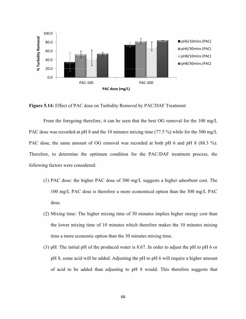
66

Figure 5.14: Effect of PAC dose on Turbidity Removal by PAC/DAF Treatment

From the foregoing therefore, it can be seen that the best OG removal for the 100 mg/L

PAC dose was recorded at pH 8 and the 10 minutes mixing time (77.5 %) while for the 300 mg/L

PAC dose, the same amount of OG removal was recorded at both pH 6 and pH 8 (88.3 %).

Therefore, to determine the optimum condition for the PAC/DAF treatment process, the

following factors were considered:

(1) PAC dose: the higher PAC dose of 300 mg/L suggests a higher adsorbent cost. The

100 mg/L PAC dose is therefore a more economical option than the 300 mg/L PAC

dose.

(2) Mixing time: The higher mixing time of 30 minutes implies higher energy cost than

the lower mixing time of 10 minutes which therefore makes the 10 minutes mixing

time a more economic option than the 30 minutes mixing time.

(3) pH: The initial pH of the produced water is 8.67. In order to adjust the pH to pH 6 or

pH 8, some acid will be added. Adjusting the pH to pH 6 will require a higher amount

of acid to be added than adjusting to pH 8 would. This therefore suggests that

0.0

20.0

40.0

60.0

80.0

100.0

PAC-100 PAC-300

% T

urbi

dity

Rem

oval

PAC dose (mg/L)

pH6/10mins (PAC)

pH6/30mins (PAC)

pH8/10mins (PAC)

pH8/30mins (PAC)

67

produced water treatment at pH 6 implies higher acid costs than treatment at pH 8

will require thus making treatment at pH 8 the more economical option.

The optimum condition for the PAC/DAF treatment scheme was therefore selected to be the 100

mg/L PAC dose at pH 8 and the 10 minutes mixing time since this condition also met the

regulatory requirement.

5.4.4. Organoclay and DAF Experiments

Effect of pH

Figure 5.15 shows that better OG removal was observed at the higher OC dose (300

mg/L) at pH 8 while better OG removal was observed at the lower OC dose (100 mg/L) at pH 6;

this was the case regardless of the mixing time. The paired t-test statistical analysis however

shows that at the higher OC dose and at both mixing times, although OG removal was better at

pH8 than pH6, the difference was not significant; p = 0.324 at the mixing time of 10 minutes and

p = 0.189 at the mixing time of 30 minutes. At the lower OC dose, the paired t-test statistical

analysis showed that OG removal at the mixing time of 30 minutes was significantly better at pH

6 than pH8 (p = 0.016) but the difference was not significant at the lower mixing time of 10

minutes (p = 0.068).

68

Figure 5.15: Effect of pH on OG Removal by OC/DAF Treatment

The OC/DAF treatment scheme also gave good turbidity removal, although it was not as

good as PAC/DAF treatment scheme, it was better than the FeCl3/DAF and control treatment

schemes. At the low OC dose (100 mg/L), better turbidity removal was observed at pH 6 (59 %)

than pH 8 (49.4 %). At the high OC dose (300 mg/L), pH did not have an impact on turbidity

removal at the 30 minutes mixing time but it had a significant impact at the 10 minutes mixing

time as the error bars suggest; again better turbidity removal was observed at pH 6 than pH 8.

This is illustrated in Figure 5.16:

Figure 5.16: Effect of pH on Turbidity Removal by OC/DAF Treatment

0.0

20.0

40.0

60.0

80.0

100.0

pH6 pH8

%O

il an

d G

reas

e Re

mov

al

pH

OC-100(10min)

OC-100(30min)

OC-300(10min)

OC-300(30min)

0.0

20.0

40.0

60.0

80.0

100.0

pH6 pH8

% T

urbi

dity

Rem

oval

pH

OC-100 (10mins)

OC-100 (30mins)

OC-300 (10mins)

OC-300 (30mins)

69

Effect of Mixing Time

Figure 5.17 shows that better OG removal is observed at the higher mixing time (30

minutes) than the lower mixing time (10 minutes) at conditions of pH and OC dose. However, as

can be seen from the figure as well as from the paired t-test statistical analysis, the difference is

not significant. The p-values for the 100 mg/L OC dose at pH 6, the 100 mg/L OC dose at pH 8,

the 300 mg/L OC dose at pH 6 and the 300 mg/L OC dose at pH 8 are 0.661, 0.550, 0.065 and

0.330 respectively.

Figure 5.17: Effect of Mixing Time on OC/DAF Treatment

Also, Figure 5.17 shows that the best OG removal results were observed with the 300

mg/L OC dose at pH 8 while the worst results were observed with the 300 mg/L OC dose at pH 6

and the 100 mg/L OC dose at pH 8.

At the low OC dose, better turbidity removal was observed at the longer mixing time (30

minutes) than the shorter mixing time (10 minutes) at both pH values (Figure 5.18) although it

was not significant; pH 6 performed better in both cases. At the high OC dose however, better

turbidity removal was observed at the shorter mixing time than the longer mixing time; pH did

0.0

20.0

40.0

60.0

80.0

100.0

10 30

% O

il an

d G

reas

e Re

mov

al

Mixing time (min)

OC-100/pH6

OC-100/pH8

OC-300/pH6

OC-300/pH8

70

not have any impact at the longer mixing time but it appeared to have a significant impact at the

shorter mixing time; pH 6 appears to perform significantly better than pH 8.

Figure 5.18: Effect of Mixing Time on Turbidity Removal by OC/DAF Treatment

Effect of OC Dose

Figure 5.19 shows that at pH 8, the higher OC dose (300 mg/L) showed better OG

removal at both the shorter (10 minutes) and longer (30 minutes) mixing times. At pH 6

however, the lower OC dose (100 mg/L) recorded better OG removal at both mixing times than

the higher OC dose. Paired t-test analysis results comparing the effect of the OC dose on OG

removal showed that OC dose did not have a significant effect on OG removal at both the low

and high pH levels and mixing times. the p values at pH 6 and 10 minutes, pH 6 and 30 minutes,

pH 8 and 10 minutes, and pH 8 and 30 minutes are, 0.155, 0.141, 0.707 and 0.295 respectively.

0.0

20.0

40.0

60.0

80.0

100.0

10 30

% T

urbi

dity

Rem

oval

Mixing Time (mins)

OC-100 (pH6)

OC-100 (pH8)

OC-300 (pH6)

OC-300 (pH8)

71

Figure 5.19: Effect of OC dose on OG Removal by OC/DAF treatment

However, we can see from Figure 5.19 that the best OG removal was observed with the

300 mg/L OC dose at pH 8 and at the mixing time of 30 minutes, with 79.5 % removal of OG

achieved. 78.1 % removal of OG was found with the OC dose of 300 mg/L at pH 8 and the

mixing time of 10 minutes. The lower OC dose at pH 6 and the mixing time of 10 minutes gave

the worst performance, with only 74 % removal of the OG.

Figure 5.19 also shows that the low and high OC doses, at both low and high pH values

as well as low and high mixing times were able to remove OG from the synthetic produced water

to meet regulatory discharge requirement of 30 mg/L; 70 % OG removal in this case. These

results confirm that OC can be used to optimise the performance of the DAF process for OG

removal from synthetic produced water.

At the shorter mixing time, the high OC dose (69.7 %) appeared to perform significantly

better at removing turbidity than the low dose (53.4 %) at pH 6. Also, at the shorter mixing time,

the high OC dose (52.8 %) produced better turbidity removal at pH 8 than the low OC dose (47.6

%) however the difference was not significant. At the high mixing time, OC dose did not have

0.0

20.0

40.0

60.0

80.0

100.0

OC-100 OC-300 % O

il an

d G

reas

e Re

mov

al

OC dose (mg/L)

Ph6/10min (OC)

pH6/30min (OC)

pH8/10min (OC)

pH8/30min (OC)

72

any impact on turbidity removal; the low OC dose actually performed better than the high dose

in this case, particularly at pH 6, although it was not significantly better.

Figure 5.20: Effect of OC dose on Turbidity Removal by OC/DAF Treatment

In order to select the optimum conditions with which to optimise the DAF unit using OC,

the performance of OC at all the factors discussed were considered. At all factors, the low OC

dose was able to aid the DAF process in removing OG to meet the regulatory discharge

requirement, hence an optimum condition of 100 mg/L OC dose at pH 6 and a mixing time of 10

minutes may be chosen as 100 mg/L OC dose may be more economical than the 300 mg/L dose.

Also, the 10 minute mixing time means more energy savings compared to the 30 minute mixing

time. However, treatment at pH 6 will require the addition of some acid in order to reduce the

produced water pH from 8.65 to 6.0, this may be a source of additional cost for this condition

hence an alternative optimum condition of 300 mg/L OC dose at pH 8 and the 10 minutes mixing

time was also considered. In this case, the higher OC dose represents more cost incurred on the

adsorbent but treating at pH 8 implies that lower acid volumes will be required to bring the

produced water pH down from 8.65 to the 8.0 range and energy savings is once again observed

by selecting the 10 minutes mixing time. The cost of OC and the acid would therefore be the

basis for deciding which of these conditions will be chosen as the optimum condition.

0.0

20.0

40.0

60.0

80.0

100.0

OC-100 OC-300

% T

urbi

dity

Rem

oval

OC dose (mg/L)

pH6/10mins (OC)

pH6/30mins (OC)

pH8/10mins (OC)

pH8/30mins (OC)

73

The 300 mg/L OC dose at pH8 and mixing time of 10 minutes was chosen as the

optimum condition because in addition to giving the better OG removal of the two conditions

compared, OC is a low cost adsorbent and so there will not be a significant impact from the cost

of the OC. Also, treating at pH 8 significantly saves acid costs.

5.4.5 Treatment Process Comparison

Figure 5.21 and Figure 5.22 summarises the results for the treatment of the synthetic

produced water for oil and grease removal and turbidity removal respectively, using the

FeCl3/DAF, PAC/DAF and OC/DAF treatment schemes.

Figure 5.21: Oil and Grease Removal with Alternative Treatment Regimes

The results of this study showed that at the high dose, PAC performed best under all

other conditions observed recording up to 88.3 % OG removal. This was followed by OC at the

300 mg/L dose at pH 8 and at the longer mixing time of 30 minutes; 79.5 % OG removal from

produced water was recorded by the OC at these conditions. The poorest performance in this

0

20

40

60

80

100

Control (DAF)

5mg/L (FeCl)

20mg/L (FeCl3)

100mg/L PAC

(10min)

300mg/L PAC

(10min)

100mg/L PAC

(30min)

300mg/L PAC

(30min)

100mg/L OC

(10min)

300mg/L OC

(10min)

100mg/L OC

(30min)

300mg/L OC

(30min)

%O

il &

Gre

ase

Rem

oval

pH6 pH8

Regulatory Limit

74

study was observed with the coagulant in which its best performance was recorded at the 20

mg/L FeCl3 dose and at both pH 8 removing 70.6 % OG from the produced water.

Under all conditions of pH, dose and mixing time, the adsorbents were able to optimise

the DAF process to reduce the residual OG content of the produced water to meet the regulatory

discharge requirement of 30 mg/L (70 % OG removal). However, only the 20 mg/L FeCl3 dose

at pH8 was able to optimize the DAF process to meet the regulatory discharge requirement.

Turbidity removal results agreed with OG removal results as illustrated in figure5.22

below.

Figure 5.22: Turbidity Removal with Alternative Treatment Technologies

0.0

20.0

40.0

60.0

80.0

100.0

Control (DAF)

5mg/L (FeCl3)

20mg/L (FeCl3)

100mg/L PAC

(10min)

300mg/L PAC

(10min)

100mg/L PAC

(30min)

300mg/L PAC

(30min)

100mg/L OC

(10min)

300mg/L OC

(10min)

100mg/L OC

(30min)

300mg/L OC

(30min)

% T

urbi

dity

Red

ucti

on

Coagulant/Adsorbant dose (mg/L) Mixing time (min) pH6 pH8

75

5.5 Conclusions

At the optimum condition of 20 mg/L FeCl3 dose and at pH8, FeCl3 was found to significantly (p

< 0.05) improve the performance of the dissolved air flotation (DAF) process for OG removal.

At the optimum condition of 100 mg/L PAC dose, pH 8 and a mixing time of 10 minutes, PAC

pretreatment was found to significantly (p < 0.05) improve the performance of the DAF process

for OG removal from produced water. At the optimum condition of 300 mg/L OC dose, pH 8

and a mixing time of 10 minutes, OC significantly (p < 0.05) improved the performance of the

DAF process for OG removal from produced water.

Organoclay is a low cost alternative adsorbent to activated carbon. Spent organoclay is

considered to be non hazardous in the United States as it does not desorb adsorbed hydrocarbon,

and as the sludge generated using organoclay is not chemical in nature, this study recommends

adsorption with organoclay as the best pre-treatment for optimizing the performance of the DAF

process in removing OG from offshore oil field produced water.

76

Chapter 6: Removal of Dissolved Oil Components with Adsorption-DAF Process

6.1 Introduction

Dissolved or soluble oil components of produced water represent all hydrocarbons and

other organic compounds that have some solubility in produced water (Arnold and Stewart,

2008). Deep-water crude has a large polar constituent, which increases the amount of dissolved

hydrocarbons in produced water. Temperature and pH can affect the solubility of organic

compounds (McFarlane et al. 2002).

Several studies presented on the chemical characterization of produced water show that

the composition is field dependent (Utvik, 1999, Utivik et. al, 2002; Brendehaug et. al, 1992;

Brown et. al. 1992) and the dissolved hydrocarbons are dominated by: the volatile aromatic

fraction of the oil namely benzene, toluene, ethylbenzene and xylene (BTEX); the polynuclear

aromatic hydrocarbons (PAHs), primarily naphthalene, phenantrene and dibenzothiophene

(NPD) and their C1-C3 alkyl homologues; phenols, which may be alkylated up to C7; and

organic acids which are dominated by C1-C6 acids (Veil et. al, 2004; Utvik, 1999). These

hydrocarbons are likely contributors to produced water toxicity, and their toxicities are additive,

so that although individually the toxicities may be insignificant, when combined, aquatic toxicity

can occur (Glickman 1998).

Generally, the concentration of organic compounds in produced water increases as the

molecular weight of the compound decreases. Produced waters from gas production have higher

contents of low molecular-weight aromatic hydrocarbons such as BTEX than those from oil

operations. Aromatic hydrocarbons and alkylated phenols are perhaps the most important

contributors to toxicity (Frost et al. 1998). Studies indicate that the produced waters discharged

from gas/condensate platforms are about ten times more toxic than the produced waters

77

discharged from oil platforms (Jacobs et al. 1992). However, for produced water discharged

offshore, the volumes from gas production are much lower, so the total impact may be less.

Due to the large droplet size of the oil present in the free and dispersed oil, they are more

easily removed by the gravity separation technologies than the dissolved oil components.

However, as oil droplet size decreases, oil removal from produced water becomes more

challenging using these technologies. Gravitational-type separation will not remove dissolved oil

from produced water (Arnold and Stewart, 2008; Veil et. al, 2004). Technologies currently being

evaluated by industry for removing soluble organics from produced water include; solvent

extraction, bio-treatment, membranes and adsorption. Benzene is normally present in higher

concentration than others in the BTEX group and analytical techniques used in their

measurement include; Purge and trap, Gas chromatography – mass spectrometry (GC-MS) and

Gas chromatography – flame ionization detector (GC/FID).

The purpose of this study was to investigate the removal of benzene with dissolved air

flotation (DAF) with coagulation or adsorption pre-treatment. Two adsorbents, PAC and

organoclay (OC) and one coagulant (ferric chloride, FeCl3) were evaluated in bench-scale

experiments to determine benzene removal efficacy of a combined coagulation-DAF and/or

adsorption/DAF process.

6.2 Materials and Methods

6.2.1 Materials

Laboratory grade benzene (chromasolv® plus, SIGMA-ALDRICH, USA) and methanol

(optima*, Fisher Scientific, Canada) were used in these experiments. Gas tight syringes

(Hamilton Company, Reno Nevada) were used for sample measurements and 2 mL gas

chromatograph auto sampler vials (Agilent Technologies, Santa Clara, USA) were used for gas

78

chromatography analysis in the 3800 Varian gas chromatograph (GC) (Agilent Technologies,

Santa Clara, USA). Ultra-pure water was obtained by using a Milli-Q system from Millipore

(Milford, M.A, USA).

6.2.2 Benzene/Methanol Stock solution

A benzene stock solution was prepared by first weighing a cleaned and dried 500 mL

sample bottle on the TP-1502 laboratory weighing balance (Denver Instruments, New York,

USA) and recording its weight. Using a dropping pipette, 2 drops of benzene were dropped into

the bottle and the bottle was weighed again to determine the weight of benzene. Methanol was

then poured into the bottle to fill it up and the bottle was weighed again to determine the weight

of the methanol. As concentration is measured in milligrams of benzene per liter of methanol, the

volume of methanol was determined from the knowledge of its mass and density, hence the

concentration of the benzene/methanol stock solution.

Standards

Using standard volumetric methods, 0.8 mL standard solutions of benzene were prepared

from two stock solutions; 231.0 mg/L and 23.1 mg/L (the 23.1 mg/L stock solution is a ten part

dilution of the 231.0 mg/L stock solution). The 231.0 mg/L stock solution was used to prepare

the standard solutions of 1, 5, 10 and 15 mg/L while the 23.1 mg/L stock solution was used to

prepare standard solutions of 0.3, 0.5 and 0.6 mg/L. The standard solutions of 0.3 and 0.6 mg/L

were prepared as quality control samples to check the level of accuracy of the calibration curve.

Also, a sample of the synthetic produced water was analyzed for its benzene content.

Volume measurements were done using 100 L and 500 L gas tight syringes into 800

L auto sampler vials. In order to avoid loss of the volatiles, the water sample was first measured

79

and transferred into the vials, and then the benzene was measured and added to it. The vial was

then fitted and sealed with the cap.

Analysis/Calibration curve

A gas chromatograph (GC) analyzer (3800 Varian) with a DB-5 column (30 m x 0.25

and auto sampler (8400 Varian) equipped with a solid phase micro extraction

(SPME) polydimethylsiloxane (100 m) fiber was used to perform the injections and measure

the concentration of benzene in solution. Headspace analysis of the 2 mL auto sampler vials were

performed with a fibre adsorption time of analytes for 5 minutes, followed by a desorption time

of 1 minute with injector temperature at 220

follows: 45 °C (0.5 min), 8 °Cmin-1 to 100 °C and 50 °Cmin-1 to 200 °C. The detector

temperature was set at 280°C, the detector type being a flame ionization detector (FID). Peak

integration of the analyses was performed using Varian Star (v. 6.20) software. Retention time

for benzene was determined to be 2.658 minutes from the benzene method on the GC.

Method Detection Limit (MDL)

The Method Detection Limit (MDL) was determined according to “The Analytical

Detection Limit Guidance and Laboratory Guide for Determining Method Detection Limits”

(Wisconsin Department of Natural Resources (1996). The MDL is the minimum concentration of

a substance that can be measured and reported with 99 % confidence that the analyte

concentration is greater than zero, and is determined from analysis of a sample in a given matrix

containing the analyte.

A new set of standards was prepared for the MDL procedure as earlier described. Results

from preliminary tests showed that benzene was present in the synthetic produced water;

80

therefore, subsequent standards were prepared using the synthetic produced water solution

instead of de-ionized water. This was done in order to account for the benzene present in the raw

water. It is also noteworthy to mention that new standards were prepared and calibration

performed every time a new measurement was to be conducted. This was done in order to ensure

the accuracy and consistency of the method.

Ten replicates of a 0.6 mg/L solution were also prepared from the stock solution.

Calibration was done and the replicate samples were analyzed for the benzene. According to the

Detection Limit Guidance and Laboratory Guide for Determining Method Detection Limits”

(Wisconsin Department of Natural Resources (1996), there are three important things to

remember about calculating MDLs; (1) use the sample standard deviation, not the population

standard deviation, (2) use the correct Student’s t-value, and (3) use all significant figures and

round the final MDL to the number of digits used when reporting results for that method. Table

6.1 summarises the results obtained from this analysis:

Table 6.1: Concentration of 0.6 mg/L Benzene standards measured by GC-FID

Sample Concentration of Benzene, X (mg/L)

1 0.5299802 0.5831313 0.5452814 0.5382755 0.5055486 0.5454647 0.5302968 0.5462659 0.49597810 0.493722

81

In order to determine the MDL the standard T-test statistical analysis was performed on

this set of data by applying the following formula (Wisconsin Department of Natural Resources,

1996).:

MDL = Standard deviation (S) x t-value Equation 6.3

The standard deviation was computed using the following formula:

Equation 6.4

Where:

X = concentration of sample (mg/L)

= mean concentration of samples (mg/L)

n = number of samples

The variables were inserted in the equation and the standard deviation, S was determined

to be 0.027. From the t distribution tables (Berthouex and Brown, 2002) the t-value for (n-1) = 9

degrees of freedom (n=10) at a probability,

Equation 6.5

Hence

The MDL was evaluated using the following five-point check (Analytical Detection Limit

Guidance, 1996):

Does the spike level exceed 10 times the MDL? If so, the spike level is high

82

Is the MDL higher than the spike level? If so, the spike level is too low

Does the calculated MDL meet regulatory requirement for the necessary program?

Is the signal/noise (S/N) in the appropriate range?

Are the replicate recoveries reasonable?

The outcome of the evaluation showed that all these checks were satisfied, however

experience has shown that the first two checks were the most important ones (Daurie 2012).

Therefore, as a spike level of 0.6 mg/L does not exceed more than 10 times the MDL and since

the MDL is not higher than the spike level, the MDL value of 0.08 mg/L was considered to be

acceptable.

Minimum Detection Limit

Having determined the instruments method detection limit, the next task was to determine the

minimum detection limit. For this task, 0.2, 0.3 and 0.4 mg/L standards were prepared from the

stock solution as well as fresh calibration standards. These concentrations were selected based on

preliminary calibration studies which showed that the 0.1 mg/L standard that was prepared, was

not detected on the calibration curve. However, standards prepared which had concentrations at

and above 0.5 mg/L were detected. Therefore, the range between 0.2 to 0.4 mg/L was chosen in

order to determine the lowest concentration that the method can be considered to accurately

measure.

Calibration was done and the results from the measurements are summarised in Table 6.2

below:

83

Table 6.2: Measured concentration of MDL samples

Sample Conc. (mg\L) Measured Conc. (mg/L)

0.2 0.247830.3 0.255250.4 0.37360

Based on the results in Table 6.2, 0.3 mg/L was selected as the Minimum Detection Limit; the

measured concentrations of the 0.3 and 0.4 mg/L samples can be seen to be approximately equal

to the sample (spiked) concentration. However, for the 0.2 mg/L sample, the measured

concentration is above the sample concentration.

6.2.3 Benzene Removal Experiments

Experiments with synthetic produced water were conducted to evaluate treatment efficacy of

coagulation and adsorption processes for removal of dissolved oil component (i.e., benzene). A

synthetic produced water sample was prepared as described in Chapter 4 and spiked with 5mg/L

of benzene solution. This concentration of benzene was chosen for these experiments because

literature shows that the average benzene concentration in produced water is within this range

(Utvik, 1999). The produced water sample was then subjected to treatment using the optimum

conditions for oil and grease removal with ferric chloride.l,l coagulant (FeCl3), powdered

activated carbon (PAC) and organoclay (OC) adsorbents determined in Chapter 5.

Coagulation/DAF and Adsorption/DAF Experiments

The optimum conditions for treating the synthetic produced water with FeCl3, PAC and OC is

summarised in Table 6.3 below:

84

Table 6.3: Optimum Coagulant and Adsorbent Pre-treatment Conditions for DAF process

Coagulant/ Adsorbent dose (mg/L) pH Mixing time (min)FeCl3 8 Rapid mix (300rpm) – 2 minutes

Slow mix (30 rpm) – 15 minutesPAC 8 10OC 8 10

For each experiment performed, four replicates of the produced water were prepared in a

1 L jar (twelve replicates in all) and the DAF unit was set up as described in Chapter 5. Of the

four samples, two samples were used as duplicates for control trials (i.e., no coagulant or

adsorbent addition) while the other two samples were used as duplicates for the coagulation\DAF

treatment and adsorption/DAF (PAC and OC) treatment respectively.

For the coagulation/DAF treatment process, the samples were first spiked with the

coagulant and their pH adjusted by spiking with the appropriate volume of acid, then the benzene

was spiked last in order to reduce the potential for benzene loss due to volatilization during

treatment. A similar approach was applied for the adsorption/DAF treatment process: the

appropriate dose of PAC/OC was first of all added to the raw water samples and their pH

adjusted by adding the appropriate amount of acid (see sections 5.2.3; PAC\DAF & OC\DAF).

Benzene was spiked last in order to reduce its loss due to volatilization.

See Chapters 3 and 5 for the applicable operating procedures and conditions for the

coagulation/DAF and adsorption/DAF treatment schemes.

85

6.3 Results

Figure 6.1 shows that by itself, DAF was able remove up to 79.3 % of the benzene

present in the produced water. The FeCl3-DAF and PAC-DAF treatment processes performed

comparatively, removing 86.6 and 86.5 % of the benzene respectively. The OC-DAF treatment

removed 83.5 % of the benzene from the produced water.

Figure 6.1: % Benzene Removal after Treatment

A comparison of each treatment scheme with the DAF treatment was done in order to

determine if they optimized the performance of the DAF process in removing benzene from the

produced water; the statistical paired t-test results show that neither coagulation (FeCl3) nor

adsorption (PAC or OC) had a significant effect on the performance of the DAF process. P

values obtained from comparing each one of the FeCl3/DAF, PAC/DAF and OC/DAF processes

with the DAF process are 0.224, 0.155 and 0.183 respectively.

Judging by the high benzene removal from the DAF treatment and subsequently from the

three treatment schemes studied, the outcomes suggests that it is possible that since benzene is a

0 10 20 30 40 50 60 70 80 90

100

DAF FeCl3 PAC OC

% B

enze

ne R

emov

al

Coagulant/Adsorbent

Benzene

86

volatile organic compound (VOC), most of the compound may have been lost due to

volatilization particularly during the DAF process.

Strictly speaking, the term VOC refers to those organic compounds which are present in

the atmosphere as gases, but which under normal conditions of temperature and pressure would

be liquids or solids. A VOC is by defnition an organic compound whose vapour pressure at say

20 °C is less than 760 torr (101.3 kPa) and greater than 1torr (0.13 kPa) (Hester and Harrison,

1995). The vapour pressure of benzene at 20 °C is 14 kPa (US Department of Health and Human

Services, 1988).

Sparingly soluble vapours partition from water into air according to Henry’s Law (Barton

et al, 2003) which states the following for a given organic compound:

Where are the equilibrium concentrations of the organic solute in the gas

and liquid phases, respectively, is the Henry’s Law constant. Henry’s Law states that the

amount of chemicals present in the air (transferred from water) is directly proportional to its

equilibrium concentration in water. It is also assumed that the solution or the mixture is ideal

(Chidgopkar, 1996). The higher the numeric value of H, the more volatile is the chemical and

hence the easier is the stripping of the chemical from water (Chidgopkar, 1996).

According to AWWA, Water Quality and Treatment (1990), several common chemicals

or pollutants found in water are categorised under A to E groups according to the ease with

which they can be stripped; the ease of stripping is in the order A > B > C > D > E. Chemicals

with high vapour pressure (i.e relatively volatile) and very low solubility have a high H value

and are therefore the easiest to strip. Benzene belongs to group B chemicals which are also easy

to strip but the process is more difficult than for category “A” chemicals. Benzene has a H value

87

of 240 atm and is classified as a group B76 chemical; the two digits describes the relative

volatility of the chemical within the group (Chidgopkar, 1996). The lower the value of the two

digit number that follows the group name, the higher the relative volatility is. Hence the

chemicals with H values ranging between 100 and 200 atm are grouped between B90 and B80.

Chemicals with H values ranging from 200 and 300 atm are grouped between B80 and B70.

The use of air flotation in the DAF process may be likened to the use of air in air

strippers, for mass transfer of volatile and semi volatile contaminants from water into the air

space (Chidgopkar, 1996). This increases the surface area between the air and the water phases

thus leading to an increase in the removal efficiency (Chidgopkar, 1996). This may explain why

such high level of benzene removal was observed from the control (DAF) treatment alone.

Hence this study suggests that although the use of the DAF process is a good option for

the removal of free and dispersed oil from produced water, it will be necessary to incorporate

such auxiliary equipment in its design as those used in air stripping for the treatment of off-gas

(usually BTEX) in order to use it for the treatment of dissolved oil in produced water; this is

necessary in order to prevent the inhalation of VOCs like benzene which are known to be

carcinogenic to humans (US Department of Health and Human Services, 1988). Such auxiliary

equipment includes activated carbon adsorption, thermal or catalytic oxidation, biological

treatment and gas-phase chemical oxidation (Stocking et.al, 2000).

88

6.4 Conclusion

The main finings of this set of experiments can be summarised as follows:

1. DAF, without pre-treatment achieved significant removal of benzene from

produced water.

2. Pre-treatment with coagulation or adsorption did not significantly impact benzene

removal in the DAF process.

3. Auxiliary equipment for treating off-gas should be incorporated in the DAF

treatment design in order to use it for the removal of dissolved VOCs (BTEX)

from produced water.

89

Chapter 7: Conclusions

7.1 Conclusions

Petroleum ether was selected as the solvent of choice of the three solvents compared for

the UV-vis spectrophotometric analysis of OG in produced water. It is not as flammable as

hexane and it is not considered to be a potentially carcinogenic to humans like dichloromethane

and it gave a comparable dissolution of crude oil as the other two solvents compared. Peak

wavelength for OG using dichloromethane, hexane and petroleum ether as solvent were found to

be at 228, 225 and 226 nm respectively.

UV-Vis spectrophotometric analytical method proved to be an alternative method for

measuring OG in oil field produced water as it gave comparable results as the FTIR

spectrometric analytical method. However, the FTIR analytical method was found to be quite

reliable for measuring both low ( 5 mg/L) and high ( 30 mg/L) OG concentrations while the

UV-Vis method was found to be reliable for measuring higher ( 30 mg/L) OG concentrations. It

was not accurate for measuring concentrations below 30 mg/L (which is the regulatory discharge

limit).

From this study, the 30 mg/L regulatory discharge limit for OG was at the 70 % OG removal

mark. By itself, the DAF process removed less than 70 % of the OG present in the oil field

produced water. At an optimum coagulant dose of 20 mg/L at pH 8, pre-treatment with ferric

chloride had a significant impact (p < 0.05) on the performance of the DAF process; 70.6 % OG

removal was achieved by the FeCl3/DAF treatment scheme. At an optimum condition of 100

mg/L PAC dose, pH 8 and at a mixing time of 10 minutes, adsorption using PAC had a

significant impact (p < 0.05) on the performance of the DAF process, removing 77.5 % OG from

the oil field produced water. At an optimum condition of 300 mg/L OC dose, pH 8 and a mixing

90

time of 10 minutes, adsorption with OC had a significant impact (p < 0.05) on the performance o

the DAF process, removing 78.1 % OG from the oil field produced water.

Organocaly is a low cost alternative adsorbent to activated carbon. Spent organoclay is

considered to be non hazardous in the United States as it does not desorb adsorbed hydrocarbon,

and as the sludge generated using organoclay is not chemical in nature, this study recommends

adsorption with organoclay as the best pre-treatment for optimizing the performance of DAF in

removing oil and grease from offshore oil field produced water.

Benzene was the target dissolved oil component in this study, however without pre-

treatment, DAF achieved significant removal of benzene from produced water which indicated

that pre-treatment with coagulation or adsorption did not significantly impact benzene removal in

the DAF process. This is because benzene is a volatile organic compound, hence similar levels of

benzene removal was observed by using the DAF process alone (79.3 %), FeCl3/DAF (86.6 %),

PAC/DAF (86.5 %) and OC/DAF (83.5 %).

Also, as benzene is known to be carcinogenic to humans, observations made from this

study suggests that although the DAF process may be a good technology for targeting the

removal of free and dispersed OG from oil field produced water, it will be necessary to

incorporate auxiliary equipment in its design, for the treatment of the off-gas (VOCs, particularly

BTEX) released during the removal of dissolved oil from the oil field produced water.

91

7.2 Recommendations

The UV-Vis analytical method has proven to be an alternative method for OG

measurement in produced water. Further studies should be performed in order to have a better

understanding of how its accuracy in measuring lower OG concentrations may be achieved. The

effect of the choice of solvent on the accuracy of the UV-Vis spectrophotometric method in

measuring low OG concentrations may also be investigated.

OG concentrations in produced water varies from field to field and geographical location,

further studies should include the investigation of the effect of varying OG concentrations on the

performance of DAF and the pre-treatment options evaluated in order to determine its effect on

the residual OG in the treated water.

Finally, in order to select the ideal pre-treatment for the DAF process, a detailed cost

analysis should be conducted.

92

References

Ahmadun, F., Pendashteh, A., Abdullah, L., Awang Biak, D., Madeni, S., & Abidin, Z. (2009). Review of technologies for oil and gas produced water treatment. Journal of Hazardous Materials 170, 530-551.

Ali, I., & Gupta, V. (2007). Advances in Water Treatment using Adsorption Technology. Nature Protocols 1, 2661-2667.

Al-Shamrani, A., James, A., & Xiao, H. (2002). Destabilization of Oil-Water Emulsions and Separation by Dissolved Air Flotation. Water Research 36, 1503-1512.

Alther, G. R. (1995). Organically Modified Clay Removes Oil from Water. Watse Management ,15 (8) 623-628.

Alther, G. (2001a). Using organoclay to enhance carbon filtration. Waste Mangement 22, 507-513.

Alther, G. (2001b). How to remove emulsified oil from wastewater with organoclays. Water Engineering and Management 7, 27-29.

APHA (American Public Health Association), AWWA (American Water Works Association), & WEF (Water Environment Federation). (2000). Standard Methods for the Examination of Water.Washington: American Health Public Association.

Arnold, K., & Stewart, M. (2008). Surface Production Operations: Design of Oil Handling Systems and Facilities. Gulf Professional Publishing.

Arthur Daniel J., Bruce G. Langhus, Chirag Patel. (2005). Technical Summary of Oil and Gas Produced Water Treatment Technologies. Tulsa, OK: ALL Consulting, LLC.

ASTM International. (2011). Standard Test Method for Oil and Grease and Petroleum Hydrocarbons in Water (ASTM, D3921-96). ASTM International.

Bansal, R. C., & Goyal, M. (2005). Activated Carbon Adsorption. Boca Raton: Taylor and Francis Group.

Barker, J. F. (1970). Chemical Engineering Sympsium Series 67, 423.

Bayati, F., Shayegan, J., & Noorjahan, A. (2012). Treatment of Oilfield Produced Water by Dissolved Air Precipitation/Solvent Sublation. Journal of Petroleum Science and Engineering,80: 26-31.

Beall, G. W. (2003). The Use of Organoclays in Water Treatment. Applied Clay Science 24,11-20.

93

Belhateche, D. (1995). Choose Appropriate Wastewater Treatment Technologies. Chemical Engineering Progress, 91 (8), 32-51.

Bennett, G. F., & Peters, R. W. (1988). The Removal of Oil from Wastewater by Air Flotation: A Review. Critical Reviews in Environmental Control 18 (3), 189-253.

Berthouex, P. M., & Brown, L. C. (2002). Statistics for Environmental Engineers (2nd Edition).Boca Raton, London, New York, Washington, D.C.: Lewis Publishers.

Betega de Paiva, L., Morales, A. R., & Valenzuela Diaz, F. R. (2008). Organoclays: Properties, Preparation and Application. Applied Clay Science 42, 8-24.

Bratby, J., & Marais, G. (1977). Flotation. In D. Purchas, Solid/Liquid Separation Equipment Scale Up (pp. 155-168). Upland Press.

Brendehaug, J., Johnsen, S., Bryne, K., Gjose, A., Eide, T., & Aarnot, E. (1992). Toxicity Testing and Chemical Characterisation of Produced Water - A Preliminary Study. In J. Ray, & F. Engelhardt, Poduced Water Technological/Environmental Issues and Solutions (p. 245). New York: Plenum Press.

Brown, J., Sauer Jr., T., Wade, M., & Neff, J. (1992). Characterisation of Produced Water Freon Extracts. In J. Ray, & F. Engelhardt, Produced Water: Technological/Environmental Issues and Solutions (p. 113). New York: Plenum Press.

Bruker Optik. (2007). Users Manual for ALPHA-T, FT-IR Spectrometer. Bruker Optik GmbH.

Callaghan, D., & Baumgartner, W. (1990). Characterisation of Residual Hydrocarbons in Produced Water Discharged from Gas Production Platforms. SPE European Petroleum Conference (pp. 22-24). The Hague: SPE.

Canada-Nova Scotia Offshore Petroleum Board. (2010). Offshore Waste Treatment Guidelines.CNSOPB.

Carey, J., Zaidi, A., & Ribo, J. (1992). Specific Toxic Organics in Produced Waters from In-Situ Havy Oil Recovery Operations in Western Canada. In J. Ray, & F. Engelhardt, Produced Water Technological/Environmental Issues and Solutions (p. 133). New York: Plenum Press.

Carrott, P., Mourao, P., Ribeiro Carrott, M., & Goncalves, E. (2005). Separating Surface and Solvent Effects and the Notion of Critical Adsorption Energy in the Adsorption of Phenolic Compounds by Activated Carbons. Langmuir , 21 (25) 11863-11869.

Carrott, P., Ribeiro Carrott, M., & Nabais, J. (1998). Influence of Surface Ioniztion on the Adsorption of Aqueous Mercury Chlorocomplexes by Activated Carbons. Carbon , 36 (1-2) 11-17.

94

Carrott, P., Ribeiro Carrott, M., Nabais, J., & Ramalho, J. (1997). Influence of Surface Ionization on the Adsorption of Aqueous Zinc Species by Activated Carbons. Carbon , 35 (3), 403-410.

Caturla, F., Martin-Martinez, J., Molina-sabio, M., Rodriguez-Reinoso, F., & Torregrosa, R. (1988). Adsorption of Substituted Phenols on Activated Carbon. J. Colloid Interface Sci. , 124, 528-534.

Caudle, D., & Stephenson, M. (1988). The Determination of Water Soluble Organics in Produced Water. New Orleans: Report to Offshore Operators Committee.

CETCO Remediation Technologies. (2012, February). Technical Data Organoclay PM-199(Organic Adsorption Media). Retrieved February 17, 2012, from Remediation Technologies: http://remediation.cetco.com/DesktopModules/Bring2mind/DMX/Download.aspx?EntryId=733&Command=Core_Download&PortalId=9&TabId=1379

Chidgopkar, V. R. (1996, March 01). Applying Henry's Law to Groundwater Treatment.Retrieved July 25, 2012, from Pollution Engineering: http://dwb4.unl.edu/Chem/CHEM869J/CHEM869JLinks/www.pollutionengineering.com/archives/1996/pol0301.96/03adp1f0.htm

Cristina, M., Almeida, M., & Vilas Boas, L. (2003). Analysis of BTEX and Other Substituted Benzenes in Water Using Headspace SPME-GC-FID Method Validation. Journal of Environmental Monitoring 6, 80-88.

Danis, T., Albanis, T., Petrakis, D., & Pomonis, P. (1998). Removal of Chlorinated Phenols from Aqueous Solutions by Adsorption on Alumina Pillared Clays and Mesoporous Alumina Aluminum Phosphates. Water Resources , 32, 295-302.

Daurie, H. (2012). Analytical Detection Limit Guidance for Benzene. Personal Communication, (K. T. Jaji, Interviewer), May 1, 2012.

Dempsey, B. A. (2006). Coagulation Characteristics and Reactions. In G. Newcombe, & D. Dixon, Interface Science in Drinking Water Treatment (pp. 5-23). Pennsylvania: Elsevier.

Dentel, S. (1996). Use of organoclay adsorbent materials for groundwater treatment applications. Delaware State Water Research Institute .

Dentel, S., Jamrah, A., & Stapleton, M. (1994). Organoclay Sorbents for Selective Removal of Organics from Water and Wastewater. In D. Wise, & D. Trantalo, Process Engineering for Pollution Control and Waste Minimization (pp. 525-534). New York: Marcel Dekker, Inc.

Doyle, D., & Brown, A. (2000). Produced Water Treatment and Hydrocarbon Removal with Organoclay. SPE Annual Technical Conferenceand Exhibition (pp. 1-11). Dallas, Texas: Society of Petroleum Engineers.

95

Duan, J., & Gregory, J. (2003). Coagulation by Hydrolysing Metal Salts. Advances in Colloid and Interface Science 100-102, 475-502.

Edwards, A., & Cresser, M. (1987). Relationship between Ultraviolet Absorbance and Total Organic Carbon in Two Upland Catchments. Water Resources , 21 (1) 49-56.

Farmaki, E., Kaloudis, T., Dimitrou, K., Thanasoulias, N., Kousouris, L., & Tzoumerikas, F. (2007). Validation of a FT-IR for the Determination of Oils and Grease in Water using Tetrachloroethylene as the Extraction Solvent. Desalination 210, 52-60.

Farmer, R., Dussert, B., & Kovacic, S. (1996). Improved Granular Activated Carbon for the Stabilization of Wastewater. Spring Symposium (pp. 456-460). Pittsburgh: Calgon Carbon Corporation.

Flentje, M., & Hager, D. (1964). Reevaluation of Granular-Carbon Filters for Taste and Odor Control. J. American Water Works Association 56, 191.

Francis, R. (1987). Water Resources 21, 1023.

Freeman, H. M. (1989). Standard Handbook of Hazardous Waste Treatment and Disposal (2nd Edition). New York: McGraw-Hill.

Frost, T., Johnsen, S., & Utvik, T. (1998). Environmental Effects of Produced Water Discharges.Norway: OLF.

Gabaldon, C., Marzal, P., Seco, A., & Gonzalez, J. (2000). Cadmium and Copper Removal by a Granular Activated Carbon in Laboratory Column Systems. Sep. Sci. Technol. 35, 1039-1053.

Glickman, A. (1998). Produced Water Toxicity: Steps You Can Take To Ensure Permit Compliance. API Produced Water Management Technical Forum and Exhibition. Lafayette, LA, Nov. 17 - 18: API.

Gopalratnam, C., Bennett, G., & Peters, R. (1988). The Simultaneous Removal of Oil and Heavy Metals from Industrial Wastewaters by Joint Precipitation and Air Flotation. Environmental Progress 7, 84-92.

Gregory, R., & Zabel, T. (1990). In F. Pontius, Water Quality and Treatment (pp. 367-453). New York: McGraw-Hill.

Gupta, V., & Suhas. (2009). Application of Low Cost Adsorbents for Dye Removal - A Review. Journal of Environmental Management 90, 2313-2342.

Hami, M., Al-Hashimi, M., & Al-Doori, M. (2007). Effect of Activated Carbon on BOD and COD Removal in a Dissolved Air Flotation Unit Treating Refinery Wastewater. Desalination216, 116-122.

96

Hanson, A., & Cleasby, J. (1990). American Water Works Association 82, 56.

Harrison, R. M. (2007). Principles of Environmental Chemistry. Royal Society of Chemistry.

Hester, R. E., & Harrison, R. M. (1995). Volatile Organic compounds in the Atmosphere. Royal Society of Chemistry.

Howe, G., Mullins, M., & Rogers, T. (1987). Evaluation and Prediction of Henry`s Law Constants and Aqueous Solubilities for Solvents and Hydrocarbon Fuel Components Vol. 1: Technical Discussion. North Carolina: Research Triangle Institute.

Imamura, K., Ikeda, E., Nagayasu, T., Sakiyama, T., & Nakanishi, K. (2002). Adsorption Behaviour of Methylene Blue and Its Congeners on a Stainless Steel Surface. J. Colloid Interface Sci. 245, 50-57.

Intertate Oil and Gas Compact and Commision ALL Consulting. (2006). A guide to practical management of produced water from onshore oil and gas operations in the United States. U.S Department of Energy National Petroleum Technology Office.

Jacobs, R., Grant, R., Kwant, J., Marqueine, J., & Mentzer, E. (1992). The Composition of Produced Water from Shell Operated Oil and Gas Production in the North Sea. In J. Ray, & F. Englehart, Produced Water: Technological/Environmental Issues and Solutions (p. 13). New York: Plenum Press.

Khaled, O., El-Sayed, M., & El-Kady, M. (2011). Treatment of Oil-Water Emulsions by Adsorption onto Activated Carbon, Bentonite and Deposited Carbon. Egyptian Journal of Petroleum 20, 9-15.

Knocke, W., West, S., & Hoehn, R. (1986). Journal of American Water Works Association 78,189.

Kuennen, R., Taylor, R., Van Dyke, K., & Groenevelt, K. (1992). Removing Lead from Drinking Water with a Point-Of-Use GAC Fixed-Bed Adsorber . J. Am. Water Works Assoc. 84, 91-101.

Kuran, P., & Sojak, L. (1996). Environmental Analysis of Volatile Organic Compounds in Water and Sediment by Gas Chromatography. Journal of Chromatography 733, 119-141.

Lalezary, S., Pirbazari, M., & McGuire, M. (1986). Evaluating Activated Carbons for Removing Low Concentrations of Taste and Odor Producing Organics. J. Am. Water Works Assoc.78, 76-82.

Lazaridis, N., Matis, K., Stalidis, G., & Mavros, P. (1992). Dissolved Air Flotation of Metal Ions. Separation Science and Technology 27, 1743-1758.

97

Lee, M., Crittenden, J., Snoeyink, V., & Ari, M. (1983). Design of Carbon Beds to Remove Humic Substances. J. Environ. Eng. ASCE 109, 631-645.

Man-Chi Lo, I., Lee, C., & Liljestrand, H. (1996). Tricaprylmethylammonium Bentonite Complexes as Adsorbents for Benzene, Toluene, Ethylbenzene and Xylene. Water Science Technology 34 (7-8) 319-325.

Marcias-Garcia, A., Valenzuela-Calahorro, C., Gomez-Serrano, V., & Espinosa-Mansilla, A. (1993). Adsorption of Pb2+ by Heat-Treated Acid Sulfurized Activated Carbon. Carbon 31,1249-1255.

McFarlane, J., Bostick, D., & Luo, H. (2002). Characterization and Modelling of Produced Water. Produced Water Conference. Colorado Springs, CO, Oct. 16-17: Ground Water Protection Council.

Morris, J., & Knocke, W. (1984). J. Am. Water Works Assoc. 76, 74.

Mourao, P., Carrott, P., & Ribeiro, C. (2006). Application of Different Equations to Adsorption Isotherms of Phenolic Compounds on Activated Carbons Prepared from Cork. Carbon , 44, 2422-2429.

Najm, I., Snoeyink, V., Lykins, B., & Adams, J. (1991). Using Powdered Activated Carbon: A Critical Review. J. Am. Water Works Assoc. 83, 65-76.

Neff, J., Sauer, T., & Maciolek, N. (1987). Fate and Effects of Produced Water Discharges in Near Shore Marine Waters, Vol. 1-2. Washington: American Petroleum Institiute.

Nikolov, A., Randie, M., Shetty, C., & Wasan, D. (1996). Chemical Demulsification of Oil in Water Emulsion using Air Flotation: The Importance of Film Thickness Stability. Chemical Engineering Communications Vols 152-153, 337-350.

Orszulik, S. T. (2008). Environmental Technology in the Oil Industry. Hampshire, U.K.: Springer.

Packham, R., & Colloid, J. (1965). Journal of Colloid & Interface Science 20, 81.

Pernitsky, D. J. (2003). Coagulation 101. Retrieved August 16/08/2012, 2012, from Alberta Water and Wastewater Operators Association: https://awwoa.ab.ca/home/pdfs/Coagulation%20101.pdf

Pinho, C., Mansilha, C., & Gameiro, P. (2011). Evaluation of the Actual Standard Procedures for Analysis of Total Extractable Hydrocarbons in Environmental Water Matrices. Desalination 273,308-315.

98

Place, M. (1991). Dissolved organic compounds in produced water. 66th Annual Technical Conference and Exhibition of the Society of Petroleum Engineers (p. SPE 22780). Texas, Dallas: Society of Petroleum Engineers Inc.

Practical Environmental Analysis (2nd Edition). Royal Society of Chemistry.

Reitz, R., & Anderson, M. (1985). Physiologically-based Pharmacokinetics and the Risk Assessment Process for Methylene Chloride. Report Prepared for the U.S Environmental Protection Agency, provided by Dr. W. Chen of Dow Chemical Canada Inc. Oct. 1985.

Richardson, J., Harker, J., & Backhurst, J. (2002). Coulson and Richardson's Chemical Engineering Volume 2 - Particle Technology and Separation Processes (5th Edition). Elsevier.

Roe, T., Johnsen, S., Frost, T., & Furnes, G. (1996). Discharges of Produced Water: Effects in the Water Column (Phase II). Stravenger, Norway.: Norweigian Oil Industry Association, OLF.

Rubio, J., Souza, M., & Smith, R. (2002). Overview of Flotation as a Wastewater Treatment Technique. Minerals Engineering 15, 139-155.

Schramn, L. L. (1992). Emulsion Fundamentals and Applications in the Petroleum Industry.Washington, DC: American Chemical Society.

Sharmasarkar, S., Jaynes, W. F., & Vance, G. F. (1999). BTEX Sorption by Montmorillonite Organoclays: TMPA, ADAM, HDTMA. Water, Air, and Soil Pollution 119, 257-273.

Simard, R., Hasegawa, I., Bandaruk, W., & Headington, C. (1951). Infrared Spectrophotometric Determination of Oil and Phenols in Water. Analytical Chemistry 23 (10) 1384-1387.

Somerville, H., Bennett, D., Davenport, J., Holt, M., Lynes, A., & Mahieu, A. (1987). Environmental Effects of Produced Water from North Sea Oil Operations. Marine Pollution Bull. 18 (10) 549-58.

Stephenson, M. (1992). Components of Produced Water: A Compilation of Industry Studies. JPT, SPE 23313, 548-603.

Stocking, A., Eylers, H., Wooden, M., Herson, T., & Kavanaugh, M. (2000). Treatment Technologies for Removal of Methyl Tertiary Butyl Ether (MTBE) from Drinking Water (2nd Edition): Air Stripping. Fountain Valley, California: Center for Groundwater Restoration and Protection, National Water Research Institute.

Strickland, W. (1980). Laborattory Results of Cleaning Produced Water by Gas Flotation. Society of Petroleum Engineering Journal 20, 175-190.

99

Tellez, G. T., Nirmalakhandan, N., & Gardea-Torresdey, J. L. (2005). Comparison of Purge and Trap GC/MS and Spectrophotometry for Monitoring Petroleum Hydrocarbon Degradation in Oilfield Produced Waters. Microchemical Journal 81, 12-18.

Tibbetts, P., Buchanan, I., Gawel, L., & Large, R. (1992). A Comprehensive Determination of Produced Water Composition. In J. Ray, & F. Engelhardt, Produced Water Technological/Environmental Issues and Solutions (p. Vol. 46 (1992) 97). New York: Plenum Press.

Tyrie, C., & Caudle, D. (2007). Produced Water Seminar - Comparing Oil in Water Measurement Methods. Exploration and Production - Oil and Gas Review (pp. 31-35). Max Oil.

U.S. Department of Health and Human Services. (2011). Report on Carcinogens. U.S. Department of Health and Human Services.

U.S. Environmental Protection Agency. (1980). EPA 440. 5-80-018: Ambient water quality criteria for benzene.

Utvik, T. (1999). Chemical Characterization of Produced Water from Four Offshore Oil Production Platforms in the North Sea. Chemosphere 39 (15) 2593-2606.

Utvik, T., Hasle, B., & Hasle, J. (2002). Recent Knowledge about Produced Water Composition and the Contribution from Different Chemicals to Risk of Harmful Environmental Effects. SPE International Conference on Health, Safety and Environment in Oil and Gas Exploration and Production (pp. 1-5). Kuala Lumpur, Malaysia: Society of Petroleum Engineers Inc.

Varian. Users Manual for Cary-100Bio UV/Vis Spectrophotometer. Varian .

Veil, John A.; Puder, Markus G.; Elcock, Deborah; Redweik, Robert J., Jr.; Argonne National Library. (2004). A White Paper Describing Produced Water from Production of Crude Oil, Natural Gas, and Coal Bed Methane. Prepared for: U.S Department of Energy National Energy Technology Laboratory.

Wisconsin Department of Natural Resources. (1996). Analytical Detection Limit Guidance and Laboratory Guide for Determining Method Detection Limits. Wisconsin Department of Natural Resources.

Yang, M., Lee, K., & Neff, J. (2011). Measurement of Oil in Produced Water. Glasgow, UK: Spring Science + Buisness Media, LLC.

Younker, J., Lee, S., Gagnon, G., & Walsh, M. (2011). Treatment of Oilfield Produced Water by Chemical Coagulation and Electrocoagulation. Offshore Technology Conference (pp. 1-5). Houston, Texas

100

Zouboulis, A., & Avranas, A. (2000). Treatment of Oil-in-Water Emulsions by Coagulation and Dissolved Air Flotation. Colloids and Surfaces 172, 153-161.

101

Appendices

Appendix A

Figure A-1: UV Absorption Spectra for Crude Oil in Hexane Standards

Figure A-2: UV Absorption Spectra for Crude Oil in Petroleum ether Standards.

0 0.2 0.4 0.6 0.8

1 1.2 1.4 1.6

200 225 250 275 300 325 350 375 400 425 450 475 500

UV-Abs

Wavelength(nm)

1mg/L

10mg/L

5mg/L

25mg/L

50mg/L

75mg/L

100mg/L

0 0.2 0.4 0.6 0.8

1 1.2 1.4

200 225 250 275 300 325 350 375 400 425 450 475 500

UV-Abs

Wavelength(nm)

1 mg/L

5mg/L

10mg/L

25mg/L

50mg/L

75mg/L

100mg/L

102

Appendix- B

Table B-1: Data, Oil & Grease Removal from Synthetic Produced Water

pH Coagulant/Adsorbent Dose (mg/L) Initial OG Concentration (mg/L) 1 2 Average % OG Removal stdevControl 92 47.6 36.6 42.1 54.2 8.4

FeCl3 - 5 33.9 34.0 34.0 62.3 0.0

FeCl3 - 20 26.9 27.2 27.1 69.9 0.2

PAC-100 (10 mins) 28.3 28.6 28.5 74.5 0.2PAC-300 (10 mins) 13.3 14.4 13.8 87.6 0.7PAC-100 (30 mins) 29.8 31.5 30.7 69.6 1.2PAC-300 (30 mins) 12.7 11.3 12.0 88.3 1.0OC-100 (10mins) 92.1 22.4 25.4 23.9 74.0 2.4OC-300 (10mins) 107.5 31.7 31.1 31.4 70.8 0.4OC-100 (30mins) 92.1 23.1 22.7 22.9 74.9 0.3OC-300 (30mins) 107.5 26.9 25.1 26.0 73.3 1.3

Control 92 54 59.2 56.6 38.5 4.0

FeCl3 - 5 27.4 30.3 28.8 68.0 2.2

FeCl3 - 20 23.0 30.0 26.5 70.6 5.5

PAC-100 (10 mins) 24.1 26.1 25.1 77.5 1.2PAC-300 (10 mins) 13.4 13.4 13.4 88.0 0.0PAC-100 (30 mins) 30.7 28.0 29.3 71.0 1.9PAC-300 (30 mins) 12.4 11.2 11.8 88.3 0.8OC-100 (10mins) 92.1 24.9 28.5 26.7 71.0 2.8OC-300 (10mins) 107.5 28.3 18.7 23.5 78.1 6.3OC-100 (30mins) 92.1 25.2 24.7 25.0 72.8 0.4OC-300 (30mins) 107.5 22.7 17.2 20.0 79.5 4.0

pH6 111.7

90

pH8

90

111.7

103

Table B-2: Data, Turbidity Removal from Synthetic Produced Water

pH Coagulant/Adsorbent Dose (mg/L) Initial Turbidity (NTU) 1 2 Average % TBD Removal stdevControl 92 48.4 54.2 51.3 44.2 2.1

FeCl3 - 5 84.6 87.4 86.0 5.5 2.1

FeCl3 - 20 80.2 68.2 74.2 18.5 9.3

PAC-100 (10 mins) 45.5 73.7 59.6 35.2 21.7PAC-300 (10 mins) 20.3 28.2 24.3 73.6 6.1PAC-100 (30 mins) 38.2 47.7 43.0 52.8 7.4PAC-300 (30 mins) 12.2 19.4 12.0 82.6 5.6OC-100 (10mins) 92 45.6 40.2 42.9 53.4 4.2OC-300 (10mins) 91 30.5 27.9 27.9 69.7 4.2OC-100 (30mins) 92 35.1 40.3 37.7 59.0 4.0OC-300 (30mins) 91 50.7 41.1 45.9 49.6 7.5

Control 92 75.5 68.3 71.9 21.8 1.1

FeCl3 - 5 78.4 76.3 77.3 15.0 1.7

FeCl3 - 20 64.8 74.1 69.4 23.7 7.2

PAC-100 (10 mins) 39.7 62.5 51.1 44.5 17.5PAC-300 (10 mins) 20.4 33.5 27.0 70.7 10.1PAC-100 (30 mins) 39.7 44.2 42.0 53.9 3.5PAC-300 (30 mins) 15.1 14.5 14.8 83.7 0.5OC-100 (10mins) 92 50.2 46.3 48.3 47.6 3.0OC-300 (10mins) 91 47.9 39.0 43.5 52.8 6.8OC-100 (30mins) 92 45.0 48.1 46.6 49.4 2.4OC-300 (30mins) 91 41.8 50.2 46.0 49.5 6.5

pH6

pH8

91

92

91

92