Thesis Crack Modelling With the EXtended Finite Element Method

Crack Modelling with the eXtended Finite Element Method

Francisco Xavier Girão Zenóglio de Oliveira

Thesis to obtain the Master of Science Degree in

Aerospace Engineering

Examination Committee

Chairperson: Prof. Fernando José Parracho LauSupervisor: Prof. Virgínia Isabel Monteiro Nabais Infante

Co-supervisor: Prof. Ricardo Miguel Gomes Simões BaptistaMembers of the Committee: Prof. Ricardo António Lamberto Duarte Cláudio

Prof. José Miguel Almeida da Silva

July 2013

II

Dedicated to my family and friends

III

IV

Agradecimentos

Deixo aqui o meu especial agradecimento a senhora professora Virgınia Isabel Monteiro Nabais

Infante, e ao senhor professor Ricardo Miguel Gomes Simoes Baptista, que sempre se revelaram

disponıveis na realizacao desta tese.

Agradeco tambem a minha famılia, que me tem sempre apoiado ao longo da minha vida academica.

Por ultimo, a todos os meus amigos, de secundario, bem como aqueles que conheci nesta casa,

Instituto Superior Tecnico, que sempre me mostraram que a vida e mais do que somente o nosso

trabalho.

V

VI

Acknowledgements

I leave here my special thanks to professor Virgınia Isabel Monteiro Nabais Infante, and professor

Ricardo Miguel Gomes Simoes Baptista, who always proved to be available in the realization of this

thesis.

I also thank to my family, who has always supported me through my academic life.

Finally, to all my friends from high school, as well as those I met in this house, Instituto Superior

Tecnico, who always showed me that life is more than just work.

VII

VIII

Resumo

O mais importante para a industria aeroespacial e a seguranca do equipamento. Os engenheiros

fazem um grande esforco para garantir elevados padroes de qualidade. O estudo de fendas e extrema-

mente importante para este proposito.

A modelacao de fendas, tem sido desde sempre um topico muito importante. As abordagens tradi-

cionais com o metodo dos elementos finitos podem fornecer solucoes precisas, no entanto, a construcao

das malhas e demorada e nao e obvia.

Um novo conceito emerge, conhecido como o Metodo de Elementos Finitos Extendidos, XFEM,

em que as descontinuidades geometricas e as sigularidades, sao introduzidas numericamente, com a

adicao de novos termos as funcoes de forma. Assim, a formulacao em elementos finitos permanece a

mesma, a representacao da fenda e mais facil, com uma solucao mais precisa.

Esta tese verifica a validade deste novo conceito para fendas estacionarias com ajuda do XFEM,

implementado no Abaqus R©. O criterio de comparacao e o factor de intensidade de tensoes para ge-

ometrias simples. Os resultados computacionais sao proximos dos valores obtidos com as solucoes

disponıveis na literatura e qualitativamente a simplicidade do metodo e verificada.

Palavras-chave: Fenda, XFEM, Abaqus R©

IX

X

Abstract

The most important thing for the aerospace industry is the equipment’s safety. Engineers, make

a great effort to guarantee high standards of quality. The study of crack phenomena is major for this

purpose.

Crack modelling, has ever been an important topic. Traditional approaches of the finite element

method can provide accurate solutions, nevertheless the meshing techniques are time consuming and

not obvious.

A new concept emerges, known as the eXtended Finite Element Method, XFEM, where the geo-

metric discontinuities and singularities, are introduced numerically with the addition of new terms to the

classical shape functions. So, the finite element formulation remains the same, the crack representation

is easier, with an approximate solution more precise.

This thesis, verifies the validity of this new concept for stationary cracks with Abaqus R©’s XFEM aid.

The comparison criterion is the stress intensity factor for simple geometries. The computational results

are near to the values obtained from the closed-forms available on the literature and qualitatively the

simplicity of this method is checked.

Keywords: Crack, XFEM, Abaqus R©

XI

XII

Table of Contents

Agradecimentos . . . . . . . . . . . . . . . . . . . . . . . . . . . . . . . . . . . . . . . . . . . . V

Acknowledgements . . . . . . . . . . . . . . . . . . . . . . . . . . . . . . . . . . . . . . . . . . VII

Resumo . . . . . . . . . . . . . . . . . . . . . . . . . . . . . . . . . . . . . . . . . . . . . . . . . IX

Abstract . . . . . . . . . . . . . . . . . . . . . . . . . . . . . . . . . . . . . . . . . . . . . . . . . XI

List of Tables . . . . . . . . . . . . . . . . . . . . . . . . . . . . . . . . . . . . . . . . . . . . . . XV

List of Figures . . . . . . . . . . . . . . . . . . . . . . . . . . . . . . . . . . . . . . . . . . . . . XVIII

Abbreviations . . . . . . . . . . . . . . . . . . . . . . . . . . . . . . . . . . . . . . . . . . . . . . XIX

Nomenclature . . . . . . . . . . . . . . . . . . . . . . . . . . . . . . . . . . . . . . . . . . . . . . XXIII

1 Introduction 1

1.1 Context . . . . . . . . . . . . . . . . . . . . . . . . . . . . . . . . . . . . . . . . . . . . . . 1

1.2 Objectives . . . . . . . . . . . . . . . . . . . . . . . . . . . . . . . . . . . . . . . . . . . . . 2

1.3 Method . . . . . . . . . . . . . . . . . . . . . . . . . . . . . . . . . . . . . . . . . . . . . . 2

1.4 Structure . . . . . . . . . . . . . . . . . . . . . . . . . . . . . . . . . . . . . . . . . . . . . 3

2 Bibliographic Research 5

2.1 Theory of Linear Elastic Fracture Mechanics . . . . . . . . . . . . . . . . . . . . . . . . . . 5

2.1.1 Stress Distribution Around a Crack . . . . . . . . . . . . . . . . . . . . . . . . . . . 5

2.1.2 Loading Modes . . . . . . . . . . . . . . . . . . . . . . . . . . . . . . . . . . . . . . 6

2.1.3 Stress Intensity Factors . . . . . . . . . . . . . . . . . . . . . . . . . . . . . . . . . 7

2.1.4 The Griffith Energy Balance . . . . . . . . . . . . . . . . . . . . . . . . . . . . . . . 8

2.1.5 The Energy Release Rate . . . . . . . . . . . . . . . . . . . . . . . . . . . . . . . . 10

2.1.6 The J-Integral . . . . . . . . . . . . . . . . . . . . . . . . . . . . . . . . . . . . . . . 11

2.2 The Finite Element Method . . . . . . . . . . . . . . . . . . . . . . . . . . . . . . . . . . . 16

2.2.1 System of Equations . . . . . . . . . . . . . . . . . . . . . . . . . . . . . . . . . . . 16

2.2.2 Constitutive Relations . . . . . . . . . . . . . . . . . . . . . . . . . . . . . . . . . . 16

2.2.3 Element Types . . . . . . . . . . . . . . . . . . . . . . . . . . . . . . . . . . . . . . 17

2.3 The Classical Approach to the Stress Intensity Factor Calculation . . . . . . . . . . . . . . 19

2.4 The eXtended Finite Element Method . . . . . . . . . . . . . . . . . . . . . . . . . . . . . 21

2.4.1 XFEM Enrichment: Jump Function . . . . . . . . . . . . . . . . . . . . . . . . . . . 21

2.4.2 XFEM Enrichment: Asymptotic Near-Tip Singularity Functions . . . . . . . . . . . 23

XIII

2.4.3 XFEM Limitations . . . . . . . . . . . . . . . . . . . . . . . . . . . . . . . . . . . . 23

3 Case Studies 25

3.1 The SENT Specimen . . . . . . . . . . . . . . . . . . . . . . . . . . . . . . . . . . . . . . . 27

3.2 The CCT Specimen . . . . . . . . . . . . . . . . . . . . . . . . . . . . . . . . . . . . . . . 28

3.3 The SENB Specimen . . . . . . . . . . . . . . . . . . . . . . . . . . . . . . . . . . . . . . 29

3.4 Cylindrical Pressure Vessel . . . . . . . . . . . . . . . . . . . . . . . . . . . . . . . . . . . 30

4 Numerical Study 33

4.1 The SENT Specimen Study . . . . . . . . . . . . . . . . . . . . . . . . . . . . . . . . . . . 33

4.1.1 Mesh Construction . . . . . . . . . . . . . . . . . . . . . . . . . . . . . . . . . . . . 33

4.1.2 Requested Contours and GRef Influence . . . . . . . . . . . . . . . . . . . . . . . 36

4.1.3 Influence of the Ratio a/W . . . . . . . . . . . . . . . . . . . . . . . . . . . . . . . . 41

4.1.4 DRef Influence . . . . . . . . . . . . . . . . . . . . . . . . . . . . . . . . . . . . . . 42

4.1.5 Interpolation and Integration . . . . . . . . . . . . . . . . . . . . . . . . . . . . . . 43

4.1.6 Standard Element Size Attribution . . . . . . . . . . . . . . . . . . . . . . . . . . . 46

4.1.7 SENT Classical Approach . . . . . . . . . . . . . . . . . . . . . . . . . . . . . . . . 47

4.1.8 SENT Discussion . . . . . . . . . . . . . . . . . . . . . . . . . . . . . . . . . . . . . 49

4.2 The CCT Specimen Study . . . . . . . . . . . . . . . . . . . . . . . . . . . . . . . . . . . . 51


4.2.2 GRef Influence . . . . . . . . . . . . . . . . . . . . . . . . . . . . . . . . . . . . . . 52


4.2.4 CCT Classical Approach . . . . . . . . . . . . . . . . . . . . . . . . . . . . . . . . . 54

4.3 The SENB Specimen Study . . . . . . . . . . . . . . . . . . . . . . . . . . . . . . . . . . . 55


4.3.2 GRef Influence . . . . . . . . . . . . . . . . . . . . . . . . . . . . . . . . . . . . . . 56


4.3.4 SENB Classical Approach . . . . . . . . . . . . . . . . . . . . . . . . . . . . . . . . 58

4.4 Vessel Under Pressure, Closed-Form Deduction . . . . . . . . . . . . . . . . . . . . . . . 59

4.4.1 The Geometry, Mesh Construction and Boundaries Conditions . . . . . . . . . . . 59

4.4.2 Results And Discussion . . . . . . . . . . . . . . . . . . . . . . . . . . . . . . . . . 62

5 Conclusions 65

5.1 Achievements . . . . . . . . . . . . . . . . . . . . . . . . . . . . . . . . . . . . . . . . . . . 65

5.2 Future Work . . . . . . . . . . . . . . . . . . . . . . . . . . . . . . . . . . . . . . . . . . . . 66

Bibliography 68

XIV

List of Tables

4.1 Impact in the average error of the requested number of contours . . . . . . . . . . . . . . 37

4.2 SENT analyses characteristics . . . . . . . . . . . . . . . . . . . . . . . . . . . . . . . . . 38

4.3 Numerical study, files appearance . . . . . . . . . . . . . . . . . . . . . . . . . . . . . . . 39

4.4 SENT GRef influence results . . . . . . . . . . . . . . . . . . . . . . . . . . . . . . . . . . 40

4.5 Ratio a/W influence for GRef=80 divisions . . . . . . . . . . . . . . . . . . . . . . . . . . 41

4.6 SENT DRef influence results . . . . . . . . . . . . . . . . . . . . . . . . . . . . . . . . . . 42

4.7 C3D8R versus C3D4R analyses characteristics . . . . . . . . . . . . . . . . . . . . . . . 43

4.8 Integration effect . . . . . . . . . . . . . . . . . . . . . . . . . . . . . . . . . . . . . . . . . 44

4.9 Standard element size attribution SENT results . . . . . . . . . . . . . . . . . . . . . . . . 46

4.10 SENT classical results . . . . . . . . . . . . . . . . . . . . . . . . . . . . . . . . . . . . . . 48

4.11 CCT analyses characteristics . . . . . . . . . . . . . . . . . . . . . . . . . . . . . . . . . . 52

4.12 CCT GRef influence results . . . . . . . . . . . . . . . . . . . . . . . . . . . . . . . . . . . 52

4.13 Standard element size attribution CTT results . . . . . . . . . . . . . . . . . . . . . . . . . 53

4.14 CCT classical results . . . . . . . . . . . . . . . . . . . . . . . . . . . . . . . . . . . . . . . 54

4.15 SENB analyses characteristics . . . . . . . . . . . . . . . . . . . . . . . . . . . . . . . . . 56

4.16 SENB GRef influence results . . . . . . . . . . . . . . . . . . . . . . . . . . . . . . . . . . 56

4.17 Standard element size attribution SENB results . . . . . . . . . . . . . . . . . . . . . . . . 57

4.18 SENB classical results . . . . . . . . . . . . . . . . . . . . . . . . . . . . . . . . . . . . . . 58

4.19 Vessel convergence evaluation, analyses characteristics . . . . . . . . . . . . . . . . . . . 60

4.20 Vessel convergence evaluation . . . . . . . . . . . . . . . . . . . . . . . . . . . . . . . . . 61

4.21 Vessel results . . . . . . . . . . . . . . . . . . . . . . . . . . . . . . . . . . . . . . . . . . . 62

5.1 Conclusions . . . . . . . . . . . . . . . . . . . . . . . . . . . . . . . . . . . . . . . . . . . . 65

XV

XVI

List of Figures

2.1 Real and ideal crack tension behaviour . . . . . . . . . . . . . . . . . . . . . . . . . . . . . 5

2.2 Stresses near the crack tip and polar coordinates . . . . . . . . . . . . . . . . . . . . . . . 6

2.3 Load modes . . . . . . . . . . . . . . . . . . . . . . . . . . . . . . . . . . . . . . . . . . . . 7

2.4 A through-thickness crack in an infinitely wide plate subjected to a remote tensile stress . 9

2.5 J-Integral, 2D contours . . . . . . . . . . . . . . . . . . . . . . . . . . . . . . . . . . . . . . 12

2.6 3D J-Integral . . . . . . . . . . . . . . . . . . . . . . . . . . . . . . . . . . . . . . . . . . . 14

2.7 Finite element domain . . . . . . . . . . . . . . . . . . . . . . . . . . . . . . . . . . . . . . 16

2.8 Abaqus R© elements . . . . . . . . . . . . . . . . . . . . . . . . . . . . . . . . . . . . . . . . 17

2.9 Degeneration of a quadrilateral element into a triangle at the crack tip . . . . . . . . . . . 19

2.10 Degeneration of a brick element into a wedge . . . . . . . . . . . . . . . . . . . . . . . . . 19

2.11 Crack-tip elements for elastic and elastic-plastic analyses . . . . . . . . . . . . . . . . . . 20

2.12 Spider-web mesh . . . . . . . . . . . . . . . . . . . . . . . . . . . . . . . . . . . . . . . . . 20

2.13 XFEM deduction, first mesh . . . . . . . . . . . . . . . . . . . . . . . . . . . . . . . . . . . 21

2.14 XFEM deduction, final mesh . . . . . . . . . . . . . . . . . . . . . . . . . . . . . . . . . . . 22

2.15 Abaqus R© enrichment scheme . . . . . . . . . . . . . . . . . . . . . . . . . . . . . . . . . . 24

3.1 Edge crack in a semi-infinite plate subject to a remote tensile stress . . . . . . . . . . . . 26

3.2 The SENT specimen . . . . . . . . . . . . . . . . . . . . . . . . . . . . . . . . . . . . . . . 27

3.3 The CCT specimen . . . . . . . . . . . . . . . . . . . . . . . . . . . . . . . . . . . . . . . . 28

3.4 The SENB specimen . . . . . . . . . . . . . . . . . . . . . . . . . . . . . . . . . . . . . . . 29

3.5 Broken pressure vessel . . . . . . . . . . . . . . . . . . . . . . . . . . . . . . . . . . . . . 30

3.6 Vessel with semicircular crack . . . . . . . . . . . . . . . . . . . . . . . . . . . . . . . . . . 31

3.7 Vessel geometry . . . . . . . . . . . . . . . . . . . . . . . . . . . . . . . . . . . . . . . . . 31

4.1 Perfectly structured mesh . . . . . . . . . . . . . . . . . . . . . . . . . . . . . . . . . . . . 33

4.2 Unstructured mesh . . . . . . . . . . . . . . . . . . . . . . . . . . . . . . . . . . . . . . . . 34

4.3 The SENT specimen final mesh . . . . . . . . . . . . . . . . . . . . . . . . . . . . . . . . . 34

4.4 Mesh refinement control . . . . . . . . . . . . . . . . . . . . . . . . . . . . . . . . . . . . . 35

4.5 Error evolution for different number of requested contours . . . . . . . . . . . . . . . . . . 37

4.6 Time evolution with the GRef parameter . . . . . . . . . . . . . . . . . . . . . . . . . . . . 39

4.7 SENT contour error evolution . . . . . . . . . . . . . . . . . . . . . . . . . . . . . . . . . . 40

XVII

4.8 Error behaviour versus a/W ratio . . . . . . . . . . . . . . . . . . . . . . . . . . . . . . . . 41

4.9 DRef influence . . . . . . . . . . . . . . . . . . . . . . . . . . . . . . . . . . . . . . . . . . 42

4.10 Stresses comparison between the two kinds of integration . . . . . . . . . . . . . . . . . . 45

4.11 Standard element size attribution, SENT absolute average error evolution . . . . . . . . . 46

4.12 Classical partition scheme . . . . . . . . . . . . . . . . . . . . . . . . . . . . . . . . . . . . 47

4.13 SENT, Classical mesh . . . . . . . . . . . . . . . . . . . . . . . . . . . . . . . . . . . . . . 47

4.14 CTT mesh . . . . . . . . . . . . . . . . . . . . . . . . . . . . . . . . . . . . . . . . . . . . . 51

4.15 CCT contour error evolution without GRef = 10 . . . . . . . . . . . . . . . . . . . . . . . . 52

4.16 Standard element size attribution, CTT absolute average error evolution . . . . . . . . . . 53

4.17 CCT classical partition scheme . . . . . . . . . . . . . . . . . . . . . . . . . . . . . . . . . 54

4.18 CCT Classical mesh . . . . . . . . . . . . . . . . . . . . . . . . . . . . . . . . . . . . . . . 54

4.19 SENB partition scheme and mesh . . . . . . . . . . . . . . . . . . . . . . . . . . . . . . . 55

4.20 SENB mesh detail . . . . . . . . . . . . . . . . . . . . . . . . . . . . . . . . . . . . . . . . 55

4.21 SENB contour error evolution . . . . . . . . . . . . . . . . . . . . . . . . . . . . . . . . . . 56

4.22 Standard element size attribution, SENB absolute average error evolution . . . . . . . . . 57

4.23 SENB classical partition scheme . . . . . . . . . . . . . . . . . . . . . . . . . . . . . . . . 58

4.24 SENB Classical mesh . . . . . . . . . . . . . . . . . . . . . . . . . . . . . . . . . . . . . . 58

4.25 Vessel geometry with boundary conditions and internal pressure . . . . . . . . . . . . . . 59

4.26 Vessel lateral view with semicircular crack . . . . . . . . . . . . . . . . . . . . . . . . . . . 59

4.27 Vessel radial stress distributions for different ESize values . . . . . . . . . . . . . . . . . . 60

4.28 Vessel geometric factor . . . . . . . . . . . . . . . . . . . . . . . . . . . . . . . . . . . . . 63

XVIII

Abbreviations

C3D4 Abaqus R© Linear Tetrahedral Element with 4 nodes

C3D8 Abaqus R© Linear Hexahedral Element with 8 nodes

C3D10 Abaqus R© Quadratic Tetrahedral Element with 10 nodes

C3D20 Abaqus R© Quadratic Hexahedral Element with 20 nodes

CAE Computed Assisted Engineering

CCT Centre Crack Tension

DOF Degrees of Freedom

DRef Depth Refinement

ESize Element Size for the Standard Element Size Attribution

FEM Finite Element Method

GRef Global Refinement

LEFM Linear Elastic Fracture Mechanics

SENB Single Edge Notch Bending

SENT Single Edge Notched Tension

XFEM eXtended Finite Element Method

XIX

XX

Nomenclature

ε Strain

Γ Contour containing the crack tip

γs Surface energy

µ Shear modulus

ν Poisson coefficient

Ω Finite domain

Φ Total energy

Π Potential energy

Ψi Crack tip asymptotic solutions

σf Fracture stress

σh Hoop stress

σij Stress tensor

σrr Radial stress

θ Polar coordinate, angle

A Crack area

a Crack length

ai Vector of enriched nodes with the Jump function

Am Amplitude, dimensionless function of θ

B Thickness

bi Vector of enriched nodes with crack tip asymptotic solutions

XXI

C Closed contour

E Young’s modulus

f Volume forces

fij Dimensionless function of θ in the leading term

G Energy release rate

H Jump function

I Identity matrix

i Number of the Depth Refinement

J J-Integral

j Number of requested contours

K Stress Intensity Factor

k Constant

Kc Fracture toughness

Ki Stress intensity factor, i mode

m Interior normal

n Exterior normal

Ni Shape functions

P Pre-logarithmic, energy factor tensor

pint Vessel internal pressure

q Vector within the virtual displacement

r Polar coordinate, radius

ro Outer radius

rp Plastic radius

ri Inner radius

S Contour area

XXII

t Tension forces

ui Displacement on the i direction

W Elastic strain energy

Ws Work necessary to create new crack faces

Y (a) Geometric factor, function of the crack length

XXIII

XXIV

Chapter 1

Introduction

1.1 Context

Nowadays, the study and evaluation of the integrity of the various mechanical components is ex-

tremely important for the industry. The two major goals are: increase the components fatigue life ex-

pectancy, and their safety.

Previously, the study and analyses were constantly made from laboratory experiments, which were

lengthy, expensive [1] and sometimes difficult to implement, due to several rules [2]. Today, there are new

materials and mechanical components appearing to a daily rhythm, which must be tested and certified

to be available for the consumers.

Inevitably, the engineers presented with systematic solutions, with higher precision, such as the

Finite Element Method, making the whole process effective and efficient. However, some mechanical

phenomena have always been difficult to model with the Finite Element Method (FEM), amongst which

the study of cracks, stationary and especially its propagation. This particular study is necessary in order

to predict the mechanical behaviour of the equipment but also in order to increase its life expectancy.

Thus, there has always been a great need of representing correctly cracks, with accurate results and

an expeditious manner. There were several attempts, which proved to be difficult to enforce for several

reasons, the main one being the mesh generation around the crack tip [1] to obtain good results. It is in

these terms that a new concept emerges recently; XFEM, eXtended Finite Element Method, creating a

new paradigm in the study of cracks [3, 4].

The method of extended elements permits a representation of cracks by finite elements, which does

not require to change the mesh to monitor crack propagation [5], causing a revolution when compared

with the classical methods. The discontinuity in the elements is described from enrichments functions

overlapping the elements.

1

1.2 Objectives

The XFEM, although a relatively recent concept, 1999, is now available in commercial versions of

finite elements. In fact, the XFEM has been already implemented in the Finite Element Method software

Abaqus R© / Standard, owned by Simulia [6].

A need therefore arises of realizing the potential and the Abaqus R©’s XFEM validity in order to un-

derstand the possibilities for subsequent analyses. The aim is thus to evaluate the XFEM for crack

modelling in Abaqus R©.

The basic idea behind the theme is to understand how accurate is the increase brought by the XFEM

in the fracture mechanics domain, to predict the integrity of mechanical systems, according to standard

methods. The main objective is to conduct a convergence analysis of the FEM discretizations, identifying

aspects and important parameters in the cases studied.

The understanding of which are the best modelling techniques with the aid of XFEM, to achieve the

best precision and efficiency within the mechanical behaviour of materials, will be the main objectives

of this thesis. So, some simulations will be performed, with solutions known by the scientific community,

using Abaqus R©’s XFEM.

1.3 Method

As first instance, it is made a bibliographic research to understand the principles of the linear elastic

fracture mechanics theory, in order to explain the calculation of the stress intensity factor; the main

parameter under analysis in this thesis. Then, the fundamentals behind the XFEM are also briefly

presented.

Next, it is done an evaluation of the XFEM in Abaqus R©, where for a given geometry, with a solution

available in the literature for its stress intensity factor, it is studied the advantages and disadvantages of

using the XFEM for different meshes, elements, rules of integration and interpolation.

Furthermore, a better validation of the XFEM is achieved with two others geometries, to verify and

confirm the conclusions from the first geometry analysis, to once again investigate the quality and appli-

cability of XFEM.

Finally, a more complex geometry is used in order to achieve a better understating of the XFEM

limitations, allowing this thesis conclusion.

2

1.4 Structure

Chapter 2 discusses initially the basic concepts of the Linear Elastic Fracture Mechanics, where it

can be understood how to calculate the stress intensity factor. In the second phase, the traditional finite

elements and their constitutive laws are presented, allowing after the introduction of the XFEM, where

its formulation is also presented.

Chapter 3 makes a brief presentation of the geometries under analysis. Their geometric character-

istics are briefly commented, and the closed-forms for theirs stress intensity factors are introduced.

In chapter 4, all the numerical analyses are carried. First, several analyses are preformed. In the end

the more important are identified in order to be better investigated with the other geometries. Finally, a

more complex structure, consisting of a vessel under internal pressure, is analysed in order to conclude

about the XFEM use for structures analysis.

Chapter 5, presents the mains conclusion of this thesis, and suggest some further works.

3

4

Chapter 2

Bibliographic Research

2.1 Theory of Linear Elastic Fracture Mechanics

2.1.1 Stress Distribution Around a Crack

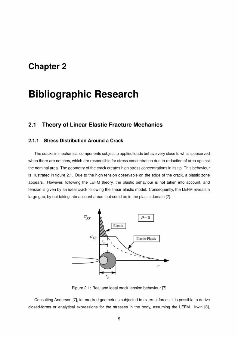
The cracks in mechanical components subject to applied loads behave very close to what is observed

when there are notches, which are responsible for stress concentration due to reduction of area against

the nominal area. The geometry of the crack creates high stress concentrations in its tip. This behaviour

is illustrated in figure 2.1. Due to the high tension observable on the edge of the crack, a plastic zone

appears. However, following the LEFM theory, the plastic behaviour is not taken into account, and

tension is given by an ideal crack following the linear elastic model. Consequently, the LEFM reveals a

large gap, by not taking into account areas that could be in the plastic domain [7].

Figure 2.1: Real and ideal crack tension behaviour [7]

Consulting Anderson [7], for cracked geometries subjected to external forces, it is possible to derive

closed-forms or analytical expressions for the stresses in the body, assuming the LEFM. Irwin [8],

5

Sneddon [9], Westergaard [10], and Williams [11] were among the first to publish such solutions.

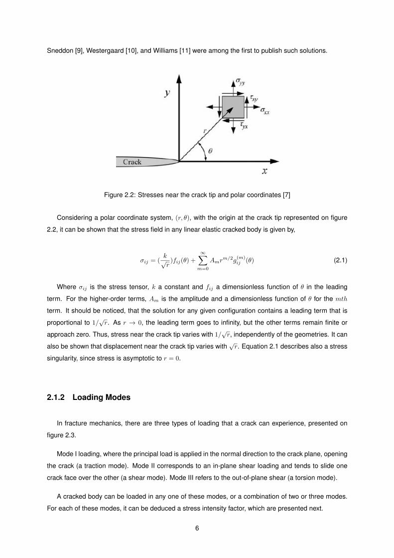
Figure 2.2: Stresses near the crack tip and polar coordinates [7]

Considering a polar coordinate system, (r, θ), with the origin at the crack tip represented on figure

2.2, it can be shown that the stress field in any linear elastic cracked body is given by,

σij = (k√r

)fij(θ) +

∞∑m=0

Amrm/2g

(m)ij (θ) (2.1)

Where σij is the stress tensor, k a constant and fij a dimensionless function of θ in the leading

term. For the higher-order terms, Am is the amplitude and a dimensionless function of θ for the mth

term. It should be noticed, that the solution for any given configuration contains a leading term that is

proportional to 1/√r. As r → 0, the leading term goes to infinity, but the other terms remain finite or

approach zero. Thus, stress near the crack tip varies with 1/√r, independently of the geometries. It can

also be shown that displacement near the crack tip varies with√r. Equation 2.1 describes also a stress

singularity, since stress is asymptotic to r = 0.

2.1.2 Loading Modes

In fracture mechanics, there are three types of loading that a crack can experience, presented on

figure 2.3.

Mode I loading, where the principal load is applied in the normal direction to the crack plane, opening

the crack (a traction mode). Mode II corresponds to an in-plane shear loading and tends to slide one

crack face over the other (a shear mode). Mode III refers to the out-of-plane shear (a torsion mode).

A cracked body can be loaded in any one of these modes, or a combination of two or three modes.

For each of these modes, it can be deduced a stress intensity factor, which are presented next.

6

Figure 2.3: Loading modes I, II and III [7]

2.1.3 Stress Intensity Factors

The stress intensity factors are used as a measure that quantifies the severity of a crack relatively

to others cracks [7]. They are so, of extreme importance for the cracks study. They are also related

to the mechanisms of crack initialization but also their propagation, and in some cases, the stress in-

tensity factor may reach an extreme value: the fracture toughness KC , leading to the fracture of the

components.

Each mode of loading produces the 1√r

singularity at the crack’s tip, but the proportionality constants

k and fij depend on the mode. For further considerations it is important to substitute k of equation 2.1

by the stress intensity factor K, where K = k√

2π . The stress intensity factor is usually given with a

subscript to denote the mode of loading, i.e., KI , KII , or KIII .

Considering the LEFM, the stress fields ahead of a crack tip in an isotropic linear elastic material can

be written as,

limr→0σ(I)ij =

KI√2πr

f(I)ij (θ) (2.2)

limr→0σ(II)ij =

KII√2πr

f(II)ij (θ) (2.3)

limr→0σ(III)ij =

KIII√2πr

f(III)ij (θ) (2.4)

For modes I, II, and III, respectively.

In a mixed-mode problem (i.e., when more than one loading mode is present), the individual contri-

butions to a given stress can be summed:

σ(Total)ij = σ

(I)ij + σ

(II)ij + σ

(III)ij (2.5)

Equation 2.5 results from the principle of linear superposition.

7

Considering this thesis will focus on loading Mode I, it is shown below both the stress and displace-

ment field ahead a crack tip,

σxx =KI√2πr

cos(θ)

[1− sin(

θ

2)sin(

3θ

2)

](2.6)

σyy =KI√2πr

cos(θ

2)

[1 + sin(

θ

2)sin(

3θ

2)

](2.7)

τxy =KI√2πr

cos(θ

2)sin(

θ

2)cos(

3θ

2) (2.8)

For plane stress,

σzz = 0 (2.9)

For plane strain,

σzz = ν(σxx + σyy) (2.10)

Where (r, θ) are the polar coordinates, ν the Poisson ratio. The remaining components of the stress

tensor are zero. For the displacement field,

ux =KI

2µ

√r

2πcos(

θ

2)

[κ− 1 + 2sin2(

θ

2)

](2.11)

uy =KI

2µ

√r

2πsin(

θ

2)

[κ+ 1− 2cos2(

θ

2)

](2.12)

Where u is the displacement, µ is the shear modulus and κ = 3− 4ν for plane strain and κ = 3−ν1+ν for

plane stress.

2.1.4 The Griffith Energy Balance

According to the first law of thermodynamics, when a system goes from a non-equilibrium state to

equilibrium, there is a net decrease in energy [7].

In 1920, Griffith applied this idea to the formation of a crack [12]:

”It may be supposed, for the present purpose, that the crack is formed by the sudden annihi-

lation of the tractions acting on its surface. At the instant following this operation, the strains,

8

and therefore the potential energy under consideration, have their original values; but in gen-

eral, the new state is not one of equilibrium. If it is not a state of equilibrium, then, by the

theorem of minimum potential energy, the potential energy is reduced by the attainment of

equilibrium; if it is a state of equilibrium, the energy does not change.”

The total energy must decrease or remain constant to form a crack or to allow its propagation. Thus

the critical conditions for fracture can be defined as the point where the crack growth occurs under

equilibrium conditions, with no net change in the total energy.

Consider a wide plate subjected to a constant stress load with a crack 2a long (figure 2.4). In order

for this crack to increase in size, sufficient potential energy must be available in the plate to overcome

the surface energy γs of the material. The Griffith energy balance for an incremental increase in the

crack area dA, under equilibrium conditions, can be expressed as follow:

dΦ

dA=dΠ

dA+dWs

dA= 0 (2.13)

Or,

dΠ

dA= −dWs

dA(2.14)

Where Φ is the total energy, Π the potential energy supplied by the internal strain energy and external

forces and Ws the work required to create new surfaces.

Figure 2.4: A through-thickness crack in an infinitely wide plate subjected to a remote tensile stress [7]

From Anderson [7], for the cracked plate illustrated in figure 2.4, Griffith [12] used the stress analysis

of Inglis to show that,

9

Π = Π0 −πσ2a2B

E(2.15)

Where Π0 is the potential energy of an uncracked plate and B is the plate thickness. Since the

formation of a crack requires the creation of two surfaces, Ws is given by

Ws = 4aBγs (2.16)

With γs the surface energy of the material. Thus,

− dΠ

dA=πσ2a

E(2.17)

And,

dWs

dA= 2γs (2.18)

Solving for the fracture stress,

σf = (2Eγsπa

)1/2 (2.19)

It is important to have in mind the distinction between crack area and surface area. The crack area is

defined as the projected area of the crack (2aB in the present example), but since a crack includes two

matching surfaces, the surface area is 2A .

2.1.5 The Energy Release Rate

Irwin [8], in 1956, proposed an energy approach for fracture that is essentially equivalent to the

Griffith model, except that Irwin approach is in a form more convenient for solving engineering problems.

Irwin defined an energy release rate G, which is a measure of the energy available for an increment

of crack extension:

G = −dΠ

dA(2.20)

The term rate, as it is used in this context, does not refer to a derivative with respect to time; G is

the rate of change in potential energy with the crack area. Since G is obtained from the derivative of a

potential, it is also called the crack extension force or the crack driving force.

10

According to equation 2.17, the energy release rate for a wide plate in plane stress with a crack of

length 2a (figure 2.4) is given by,

G =πσ2a

E(2.21)

Referring to the previous section, the crack extension occurs when G reaches a critical value,

Gc =dWs

dA= 2γs (2.22)

Where Gc is also a measure of the fracture toughness of the material.

At this moment, it must be said the energy release rate is extremely important for this thesis. This is

justified by its direct relationship with the stress intensity factor.

Irwin’s showed that for linear elastic materials, under loading Mode I, it may be written,

G =K2I

E′(2.23)

Where for plane stress,

E′ = E (2.24)

And for plane strain,

E′ =E

1− ν2(2.25)

Nevertheless, the energy release rate is still not enough and practical to get the value of the stress

intensity factor.

2.1.6 The J-Integral

In the previous section, it was showed the basis behind the energy release rate, with a direct relation

with the stress intensity factor. Even the energy release rate is a simple concept, it is not obvious how

to deduce it with the finite element method. Fortunately, there is another concept in the LEFM theory,

called the J-Integral, which may be calculated numerically and reveals itself very useful because in the

context of LEFM, the J-Integral is equal to the energy release rate G.

11

J-Integral Calculation

As said before, the stress intensity factor can be calculated by the energy release rate G, which in

this thesis context is equal to the J-Integral.

The J-Integral is a contour integral for bi-dimensional geometries (see figure 2.5). Its definition is

easily extended to three-dimensional geometries, and it is used to extract the stress intensity factors.

Figure 2.5: a) 2D contour integral, b) 2D closed contour integral [6]

For the two-dimensional case, the J-Integral is given by,

J = limΓ→0

∫Γ

n.H.qdΓ (2.26)

Where Γ is the contour containing the crack tip, n is the exterior normal to the contour, and q is the

unitary vector within the virtual displacement direction of the crack.

The function H is defined by,

H = WI − σ.∂u∂x

(2.27)

Where W is the elastic strain energy1, I the identity tensor, σ the stress tensor and u the vector of

displacements.

The contour Γ connects the two crack faces and encloses the crack tip. This is shown in figure 2.5

a). The contour tends to zero, until it only contains the crack tip (equation 2.26). The exterior normal n

moves along the integration while q stands fixed in the crack tip.

1The strain energy definition may also include the elastic-plastic effects, which are not presented, considering the fact that theywill not be subject in this thesis.

12

It is very important to note the J-Integral is independent of the chosen path for elastic materials in the

absence of imposed forces in the body or tension applied on the crack, so the contour does not need to

contract itself on the crack, but it has only to enclose the crack tip.

The two dimensional integral may be rewritten as a closed bi-dimensional contour integral as the

following [13],

J = −∮C+C−+C++Γ

m.H.qdΓ−∫C++C−

t.∂u

∂x.qdΓ (2.28)

Where the line integrals are preformed in a closed contour, which is an extension of Γ. C+ and C−

are contours along the crack faces, enclosed by C. The normal m had to be introduced as the unitary

exterior normal to the contour C, respecting m = −n. The function q had also to be introduced, being a

unitary vector applied in the direction of the virtual extension of the crack tip, which respects q = q in Γ

and vanishes in C.

In equation (2.28), t is the tension on the crack faces. Crack tension is also a subject not considered

in this thesis. The second term may be erased from equation 2.28.

The J-Integral may be now transformed in a surface integral by the divergence theorem properties,

yielding to,

J =

∫S

(∂

∂x).(H.q)dS (2.29)

Where S is the area in the closed domain. The equilibrium forces equation is,

(∂

∂x).σ + f = 0 (2.30)

Where σ is the tension tensor, and f the volume forces. And the energy strain gradient, for an

homogeneous material with constant properties is,

(∂W (ε)

∂x) =

∂W

∂ε

∂ε

∂x= σ

∂ε

∂x(2.31)

Where ε is the mechanical strain.

Considering these two previous equations, the J-Integral may now be written as,

J = −∫S

(

[H∂q

∂x+ (f.

∂u

∂x).q

])dS (2.32)

The bi-dimensional equation for the J-Integral is easily extended to a three dimensional formulation.

The J-Integral has to be defined in order to a parametric variable s, in the crack front, in such manner

13

J(s) is defined by a function which characterizes the bi-dimensional J-Integral for each point placed in

the path defining the crack front, which is also described parametrically in order to s (figure 2.6).

Figure 2.6: a) Local coordinates system, b) 3D J-Integral [6]

The local system of cartesian coordinates is placed in the crack front. See figure 2.6 a). The axis

x3, runs tangentially the crack, x2 is defined perpendicular to the crack front. In this formulation, x1 will

always be directed forward at the crack front. x1 and x2 define a perpendicular plane to the crack front.

J(s) is so described in the x1x2 plane.

From figure 2.6, it is obvious that for the three-dimensional case, each infinitesimal 2D contour must

be integrated, for each position of s, along the path described by the crack front in order to obtain a

volume J-Integral.

Stress Intensity Factors Extraction

Having defined the procedure to obtain the J-Integral, for both, bi-dimensional and three-dimensional

crack geometries, it becomes necessary to extract the stress intensity factors. Consulting Abaqus R©

Documentation [6], for a linear elastic material, the J-Integral is related to the stress intensity factors by

the following relation,

J =1

8πKTP−1K (2.33)

With K = [KI ,KII ,KIII ]T and P the pre-logarithmic energy factor tensor [14, 15, 16, 17].

For homogeneous and isotropic materials this equation may be simplified in the form,

14

J =1

E′(K2

I +K2II) +

1

2GK3III (2.34)

Where, E′ is given by equations 2.24 and 2.25.

At last, for pure Mode I loading, the relation between the J-Integral and the stress intensity factor is

given by,

J = (K2I

E′) (2.35)

Which is exactly the equation presented in section 2.1.5.

15

2.2 The Finite Element Method

2.2.1 System of Equations

In this section, are presented the governing equations of the finite elements, used for the analyses.

Figure 2.7: FEM domain and boundary condtions [5]

Considering the domain Ω of figure 2.7, the border Λ may be divided in four independent borders: Λt

with tension applied, Λu with imposed displacements, and the last two domains,Λ+c and Λ−c , representing

the crack faces.

The equilibrium equations and boundary conditions are,

∇σ + f = 0 in Ω (2.36)

σ.n = t in Λt (2.37)

σ.n = 0 in Λ+c (2.38)

σ.n = 0 in Λ−c (2.39)

u = uimp in Λu (2.40)

Where f represents the volume forces, n the outer normal, t the superficial forces, uimp the imposed

displacements. Finally, considering an infinitesimal deformation δv, the weak formulation is,

∫Ω

σ∇δv =

∫Λt

tδvdΓ +

∫Λ

fδvdΩ (2.41)

2.2.2 Constitutive Relations

Although the fact the weak formulation has always the same form, the element quality depends on

the constitutive relations, as well of the selected shape forms.

This thesis is limited to the linear elastic fracture mechanics, implying that only small strains will be

considered. The material model could not be different than the presented next, which is a limitation

imposed by the commercial software of analysis Abaqus R©, allowing only this model for XFEM aid.

16

Respecting the elasticity theory, the tension obeys to the following,

σxx

σyy

σzz

σxy

σxz

σyz

= D

εxx

εyy

εzz

2εxy

2εxz

2εyz

(2.42)

Being D given by,

D =E(1− ν)

(1 + ν)(1− ν)

1 ν1−ν

ν1−ν 0 0 0

ν1−ν 1 ν

1−ν 0 0 0

ν1−ν

ν1−ν 1 0 0 0

0 0 0 1−2ν2(1−ν) 0 0

0 0 0 0 1−2ν2(1−ν) 0

0 0 0 0 0 1−2ν2(1−ν)

(2.43)

Where σij and εij are the tension and strain components, E the Young’s modulus, and ν the Poisson

coefficient.

2.2.3 Element Types

In Abaqus R©, the geometries under analysis can be modelled with two types of volumetric ele-

ments: the tetrahedral and hexahedral, which remains the isoparametric element most used for three-

dimensional elasticity [18].

Abaqus R© admits two formulations of this element. The linear element of 8 nodes, identified as C3D8,

and the quadratic of 20 nodes, C3D20 (figure 2.8 a and b).

At each node, for both elements, there are three degrees of freedom, corresponding to three possible

displacements. Thus, the element of 8 nodes, has 24 degrees of freedom, a number three times lower

than the 60 degrees of freedom of the element of 20 nodes [6].

Figure 2.8: Three dimensional elements, (a) 8 nodes, (b) 20 nodes, (c) 10 nodes, from [6]

17

As for the tetrahedral, there is a linear element of 4 nodes, C3D4 and a quadratic element with 10

nodes, the C3D10 (figure 2.8 c).

Any of the four elements allows two kinds of numerical integration; reduced or full integration. The

reduced integration is identified by a R in the element code. For example, C3D20R, indicates a three-

dimensional element of 20 nodes, being a quadratic with reduced integration.

18

2.3 The Classical Approach to the Stress Intensity Factor Calcu-

lation

In order to have a full understanding of the XFEM, it is necessary to evaluate the geometries with the

classical approach for the stress intensity factor calculation.

In the classical approach, according to [7], in two-dimensional problems quadrilateral elements are

collapsed to triangles where three nodes occupy the same point in space, like what is shown on figure

2.9. For three dimensions problems, a brick element is degenerated to a wedge (figure 2.10).

Figure 2.9: Degeneration of a quadrilateral element into a triangle at the crack tip [7]

Figure 2.10: Degeneration of a brick element into a wedge [7]

In elastic problems, the nodes at the crack tip are normally tied, and the mid-side nodes moved to the

1/4 points. This modification is necessary to introduce a 1/√r strain singularity in the element, which

brings numerical accuracy due to the fact that the analytical solution contains the same term.

A similar result can be achieved by moving the midside nodes to 1/4 points in non collapsed quadri-

lateral elements, but the singularity would exist only on the element edges; collapsed elements are

preferable in this case because the singularity exists within the element as well as on the edges.

When a plastic zone forms, the singularity no longer exists at the crack tip. Consequently, elastic

singular elements are not appropriate for elastic-plastic analyses. Figure 2.11 shows an element that

exhibits the desired strain singularity under fully plastic conditions.

19

Figure 2.11: Crack-tip elements for elastic and elastic-plastic analyses. Element (a) produces a 1/√r

strain singularity, while (b) exhibits a 1/r strain singularity (a) Elastic singularity element and (b) plasticsingularity element [7]

According to [1], [6] and [7], for typical problems, the most efficient mesh design for the crack-tip

region is the “spider-web” configuration (figure 2.12), consisting of concentric rings of quadrilateral ele-

ments that are focused toward the crack tip. The elements in the first ring are degenerated to triangles,

as described above. Since the crack tip region contains stress and strain gradients, the mesh refinement

should be greater at the crack-tip. The spider-web design allows a smooth transition from a fine mesh

at the tip to a coarser. In addition, this configuration results in a series of smooth, concentric integration

domains (contours) for the J-Integral calculation.

Figure 2.12: Spider-web mesh from [6]

20

2.4 The eXtended Finite Element Method

The extended finite element method, XFEM, is an evolution of the classical finite element method

based on the concept of partition unit, i.e. the sum of shape functions is equal to one.

This method was initially developed by Ted Belytschko [3] and his colleagues in 1999. The XFEM

based on the concept of partition of unity [19], adds a priori known information about the solution of a

given problem, to the FEM formulation, making possible, for example, to represent discontinuities and

singularities, independently of the mesh. This particular feature makes this method very robust and

attractive to simulate the propagation of cracks, since it is no longer necessary to have a continual

updating of the mesh. The XFEM is then referenced as a Meshless method.

In the XFEM, enrichment functions are added to additional nodes, in order to include information

about discontinuities and singularities around the crack. These functions are the asymptotic near-tip

solutions, which are sensitive to singularities, and the Jump function, which simulates the discontinuity

when the crack opens.

2.4.1 XFEM Enrichment: Jump Function

To explain the form how the discontinuities are added to the FEM, consider a simple bi-dimensional

geometry (figure 2.13), with four elements and an edge crack.

Figure 2.13: Bi-dimensional geometry for the XFEM deduction

The solution for the displacement is typically given by,

u(x, y) =

10∑i=1

Ni(x, y)ui (2.44)

Where Ni(x, y) is the shape function on node i with coordinates (x, y), and ui is the displacement

vector.

21

Defining c as a middle point between u9 and u10 and d as the distance between the two nodes, it is

possible to write,

c =u9 + u10

2(2.45)

d =u9 − u10

2(2.46)

But also,

u9 = c+ d (2.47)

u10 = c− d (2.48)

Manipulating the expression 2.44,

u(x, y) =

8∑i=1

Ni(x, y)ui + c(N9 +N10) + d(N9 +N10)H(x, y) (2.49)

Where the Jump function was added obeying to,

H(x, y) =

1 y > 0

−1 y < 0

(2.50)

We may substitute (N9 +N10) by N11 and c by u11.

Figure 2.14: Bi-dimensional geometry, the final mesh, with the new node

The displacement approximation becomes,

22

u(x, y) =

8∑i=1

(Ni(x, y)ui +N11u11) + (dN11H(x, y)) (2.51)

The first term of the equation is the conventional approximation by the FEM, and the second term cor-

responds to the Jump enrichment, associated to a new node, with displacement u11, and consequently

new degrees of freedom.

The equation 2.51, reveals that the geometry crack can then be represented by a mesh which does

not contain any discontinuity, since this is included in the equation due to the presence of the enrichment

term reproducing the crack discontinuity.

2.4.2 XFEM Enrichment: Asymptotic Near-Tip Singularity Functions

In the previous section, it was shown which enrichment function can capture the discontinuity due to

the presence of a crack or notch. It remains to illustrate how to pick up the singularities existing in this

type of problem. The enrichment function appointed above, will be introduced in all the elements around

the crack. However, the following asymptotic solutions will be introduced only at the crack tips.

Let all nodes be represented by the set S, the nodes that comprise the tips are the set Sc and the

other, comprising the physical discontinuity, are the set Sh.

The approximation becomes,

u(x, y) =

8∑i∈S

Ni(x, y)(ui +H(x, y)aii∈Sh

+

4∑i=1

ψi(x, y)bi

i∈Sc

) (2.52)

Where ui is the nodal displacement, ai represents the vector of enriched nodes with the discontinuity

function, and bi are the nodes enriched with the crack tip asymptotic solutions.

The enrichment functions at the crack tips, for linear elastic isotropic materials are given by,

ψi(x, y)4i=1 = (√rsin(α),

√rcos(α/2),

√rsin(α/2)sin(α),

√rcos(α/2)sin(α)) (2.53)

Where (r, α) correspond to the polar coordinates of point with Cartesian coordinates (x, y).

2.4.3 XFEM Limitations

Although the XFEM has been developed for the study of static or propagating cracks, this work will

focus mainly on the static case, since crack propagation is even complex and heavy in computational

terms, with numerical convergence issues. Moreover, for propagating cracks, the asymptotic near-tip

singularity functions are not included in the enrichment scheme (figure 2.15).

23

Figure 2.15: Abaqus R© enrichment schemes for both, stationary and propagating cases [20]

Another limitation relates to the fact that all the geometries presented are three-dimensional since

the considered Abaqus R© version (CAE 6.12) does not allow the calculation of the stress intensity factor

in two-dimensional geometries with XFEM use.

All simulations will assume linear elastic materials and the theory of linear elastic fracture. This

limitation is imposed by the Abaqus R©, which only allows stationary analysis with linear elastic materials,

since Abaqus R© 6.12 only contemplates the near-tip asymptotic solutions for the stress field at the crack’s

tip for isotropic linear elastic material.

24

Chapter 3

Case Studies

This thesis purpose is to validate the XFEM in the context of mechanical behaviour, most precisely,

the fracture mechanics. The most interesting parameter to consider is the stress intensity factor; a value

very useful to quantify the crack importance on the stress distribution. In order to emphasize the possible

advantages or disadvantages brought by the XFEM, it must be investigated the quality of the solutions

with XFEM aid. From Anderson [7], it is very hard to find the closed-forms or analytical solutions for

the stress intensity factor of a given loaded geometry. Nevertheless, there are still some solutions for

very simple configurations. For the more complex geometries, the stress intensity factor must be derived

numerically, by finite elements. For example, one configuration for which a closed-form solution exists is

a through crack in an infinite plate subjected to a remote tensile stress (figure 2.4). It can be shown the

solution in this case, is given by,

KI = Y (a)σ√πa (3.1)

Y (a) = 1 (3.2)

Thus the amplitude of the crack-tip singularity for this configuration is proportional to the remote

stress and the square root of the crack size. Note this solution is for a infinite body, turning it useless for

this thesis. There is also a related solution for a semi-infinite plate with an edge crack, figure 3.1, from

[7].

This configuration can be obtained by slicing the plate in figure 2.4 through the middle of the crack.

The stress intensity factor for the edge crack is given by,

KI = 1.12σ√πa (3.3)

This is very close to equation 3.1. The 12% increase in KI for the edge crack is caused by different

boundary conditions at the free edge. As figure 3.1 illustrates, the edge crack opens more because it

25

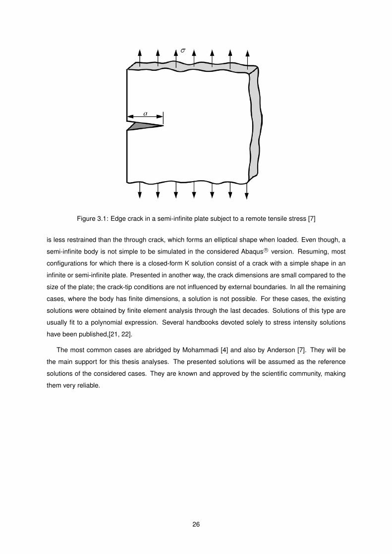
Figure 3.1: Edge crack in a semi-infinite plate subject to a remote tensile stress [7]

is less restrained than the through crack, which forms an elliptical shape when loaded. Even though, a

semi-infinite body is not simple to be simulated in the considered Abaqus R© version. Resuming, most

configurations for which there is a closed-form K solution consist of a crack with a simple shape in an

infinite or semi-infinite plate. Presented in another way, the crack dimensions are small compared to the

size of the plate; the crack-tip conditions are not influenced by external boundaries. In all the remaining

cases, where the body has finite dimensions, a solution is not possible. For these cases, the existing

solutions were obtained by finite element analysis through the last decades. Solutions of this type are

usually fit to a polynomial expression. Several handbooks devoted solely to stress intensity solutions

have been published,[21, 22].

The most common cases are abridged by Mohammadi [4] and also by Anderson [7]. They will be

the main support for this thesis analyses. The presented solutions will be assumed as the reference

solutions of the considered cases. They are known and approved by the scientific community, making

them very reliable.

26

3.1 The SENT Specimen

The first geometry to be considered for the analysis is known as the SENT specimen, an acronym

for Single Edge Notched Tension plate. It consists of a parallelepiped specimen with a corner crack in

its longitudinal symmetry axis. The choice of this specimen to the first analysis is due to its popularity

in experimental studies of fracture mechanics. Due to this fact, this sample is likely to have an accurate

empirical solution for the stress intensity factor.

Figure 3.2: The SENT specimen

As can be seen in the figure 3.2, the sample has a height H, width W , an edge crack of width a, and

thickness B. The solution for the stress intensity factor of this specimen, accessed in [4], is given by,

KI = Y (a)σ√πa (3.4)

Y (a) = [1.12− 0.23(a

W) + 10.56(

a

W)2 − 21.74(

a

W)3 + 30.42(

a

W)4] (3.5)

This specimen is the basis of study for most of the analyses presented in this thesis. The results

obtained for the different analysis performed in this specimen, allow the study of the others geometries,

with superior knowledge about XFEM.

27

3.2 The CCT Specimen

The second specimen considered for the numerical investigation is another one very popular among

the scientific community identified as CCT, an acronym for Center Crack Tension plate. The stress

intensity factor for a through crack 2a long, at right angles, in an infinite plane, with an uniform stress

field applied, is given by the equation 3.1.

Figure 3.3: The CCT specimen

Considering the figure 3.3, the specimen has a height H, width W , and a centre crack 2a long.

Consulting [4], the stress intensity factor is,

KI = Y (a)σ√πa (3.6)

Y (a) = [1 + 0.256(a

W)− 1.152(

a

W)2 + 12.2(

a

W)3] (3.7)

28

3.3 The SENB Specimen

The last considered specimen is the Single Edge Notch Bending specimen, identified by the acronym

SENB. This one, unlike the others presented, is not under traction load but in bending, caused by a three

point load apply.

Figure 3.4: The SENB specimen [7]

The specimen is horizontally positioned, with three forces applied; P on the bottom, and P/2 on each

of the two top corners. The span is S = 4W , contrasting with the height W . The thickness is B.

From Bower [23],

KI =4P

B

√π

W

[1.6(

a

W)1/2 − 2.6(

a

W)3/2 + 12.3(

a

W)5/2 − 21.2(

a

W)7/2 + 21.8(

a

W)9/2

](3.8)

29

3.4 Cylindrical Pressure Vessel

After the validation of the XFEM with the previous specimens, with the acquired knowledge, it will be

deducted a closed-form solution for a cylindrical vessel under pressure.

Cylindrical vessels, under internal pressure, are commonly used in many engineering applications.

They may be used as industrial compressed air receivers and domestic hot water storage tanks. Other

examples of pressure vessels are the distillation towers, pressure reactors, autoclaves. They are also

present in oil refineries and petrochemical plants, nuclear reactor vessels, submarine, aircraft and space

ship habitats, and storage vessels for liquified gases such as ammonia, chlorine, propane, butane, and

LPG.

Due to fatigue loads, vibrations and thermal stresses, the vessels are affected by crack initiation and

propagation until the inevitable fracture (figure 3.5).

Figure 3.5: Broken pressure vessel <http://www.pjedwards.net/>

The existence of closed-forms for the stress intensity factors in vessels are of extreme importance.

With this structure, the goal is to preform a set of analyses, producing a closed-form under certain

conditions, and compare it with one existing solution.

For a semicircular crack (figure 3.6 with c = a), from [24], the closed-form solution is,

KI = 1.122

πσh√πa (3.9)

Where σh is the hoop stress, and a the crack radius. The hoop stress, is related with the internal

pressure. Assuming a thin vessel, stress-plane conditions may be assumed and so there is only two

30

<http://www.pjedwards.net/>

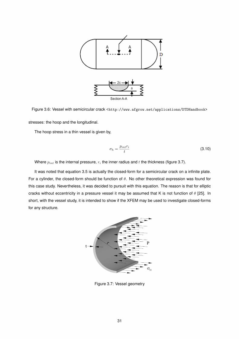
Figure 3.6: Vessel with semicircular crack <http://www.afgrow.net/applications/DTDHandbook>

stresses: the hoop and the longitudinal.

The hoop stress in a thin vessel is given by,

σh =pintrit

(3.10)

Where pint is the internal pressure, ri the inner radius and t the thickness (figure 3.7).

It was noted that equation 3.5 is actually the closed-form for a semicircular crack on a infinite plate.

For a cylinder, the closed-form should be function of θ. No other theoretical expression was found for

this case study. Nevertheless, it was decided to pursuit with this equation. The reason is that for elliptic

cracks without eccentricity in a pressure vessel it may be assumed that K is not function of θ [25]. In

short, with the vessel study, it is intended to show if the XFEM may be used to investigate closed-forms

for any structure.

Figure 3.7: Vessel geometry

31

<http://www.afgrow.net/applications/DTDHandbook>

32

Chapter 4

Numerical Study

4.1 The SENT Specimen Study

The study and the validation of this new method have not proven to be an easy task because of the

large number of parameters which need to be evaluated. Organize and structure the agenda proved to

be a complex point. In this section, using the SENT specimen, it is presented and discussed the results

for different aspects of this validation.

4.1.1 Mesh Construction

Bearing in mind the XFEM, it is known in advance, from the bibliographic research [26], that the

mesh should be orthonormal around the crack. Moreover, it should have a high density, leading to more

accurate results [26]. Thus, considering hexahedral elements in the first instance, a perfectly structured

mesh is chosen as first approach (figure 4.1).

Figure 4.1: Perfectly structured mesh.

Although not evident, the mesh represented on figure 4.1, is quite poor. If it was a problem of

displacement calculation, it would probably suffice. However, it is intended here to calculate the stress

33

intensity factor, which requires a much finer mesh around the crack.

Imposing a better refinement, leading to a sufficiently fine mesh, the solving process becomes quite

heavy in time. Running a very fine mesh, appears very difficult for a common user laptop, as the one

that was used for this thesis realization. It is then necessary to find a mesh that obey to all the criteria

for the analyses and which is not too expensive in computational time.

It was chosen to partition the mesh [6]. In other words, the mesh is defined by blocks, where each

block has a proper refinement. However, after preliminary testing for convergence, the mesh defined

by blocks may pose some problems. Sometimes, for a given partition scheme, the Abaqus R© meshing

algorithms are forced to build unstructured meshes with degenerated elements (figure 4.2), which makes

the mesh weak with a consequent loss of accuracy.

Figure 4.2: Unstructured mesh

A structured mesh, with high density around the crack, is really necessary for good results. It should

be noted at this point that for the Abaqus R©, a structured mesh, is not necessarily a mesh with orthonor-

mal elements. In Abaqus R©, a structured mesh, must verify that all the elements have a parallelogram

shape in 2D and a hexahedral shape in 3D.

After consultation of [7] and an optimisation study, the partition scheme presented on figure 4.3 was

derived. This partition allows a fine refinement near the crack, and a coarser mesh for the remaining

points.

Figure 4.3: SENT final mesh.

34

This partition scheme generated structured meshes in all simulations. It is noted however that when

the specimen has its height H or too low or too high, the distorted elements begin to increase. Those

elements do not introduce a significant error since they are situated in the far-field.

In addition to this partition scheme, two edges sets were defined: the Global Refinement, which

assigns to all the edges in the plane the introduced number of divisions, and the Depth Refinement,

which controls the refinement of all the elements responsible of the three-dimensionality. It can be

appreciated in figure 4.4 the consequence of these parameters variation.

Figure 4.4: Mesh refinement control: a) Global Refinement of 10 with Depth Refinement of 1 b) GlobalRefinement of 10 with Depth Refinement of 10

The crack block is the block around the crack. It is always used a square as block, with a characteristic

dimension corresponding to the double of the crack length. This block definition has been validated from

several analysis, proving to be the one with less oscillations in the majority of the different solutions.

The greatest advantage of all, with this mesh design, it is logically the high density around the crack

which is essential, since it is a point of accumulation of stresses, with high gradients, requiring a higher

number of nodes. For instance if the Global Refinement is fixed at a value of 20 there will be in the crack

block 400 elements in the plane.

35

4.1.2 Requested Contours and GRef Influence

As mentioned in section 2, the J-Integral, that allows the stress intensity factor deduction, is calcu-

lated by 2D closed contour integrals. In theory, the J-Integral is path independent, but numerically (or

computationally) this is not true. Thus, different contours give different solutions for the stress intensity

factor.

Abaqus R© allows the user to introduce the number of contours to use for the stress intensity factor

calculation, but what number should be introduced? Furthermore, it was observed that the package of

requested contours is calculated for each of the generated points in the crack’s front.

The number of generated points, appears to be related to the number of mesh divisions in depth. For

structured geometries, if the geometry is a parallelepiped and has i divisions in depth, there will be i+ 1

point, which implies i+ 1 packages of j contours, each one with a stress intensity factor estimation.

Against this backdrop, it was necessary to design a set of tests that could clarify various doubts. A

large sample of analysis was needed in order to be able to understand how to tune the parameters to

obtain good results.

Choosing then a SENT geometry, which was set with a height H = 90 mm, width W = 10 mm, crack

length a = 2 mm, it was made the study of the computational burden associated to the mesh variations.

In terms of thickness, B = 1 mm, and only 2 divisions in depth were considered. For the elements, it

was used hexahedral elements with first order accuracy, and reduced integration, since as it is shown

later on this thesis, these characteristics are the best choice.

As previously stated, two sets of refinement were defined, Global Refinement and Depth Refinement,

referred to from now on as GRef and DRef. In this set of analyses, the first will vary and the second will

be fixed in 2 divisions. The partition scheme remains constant, so the increase of GRef , increases the

mesh density around the crack.

Another question arises now. What will be the composition of the solution since each contour pro-

vides a different value for the stress intensity factor? And which contours should be chosen? All of them

or only some?

In all the existing Computed Assisted Engineering (CAE) solutions, regarding the stress intensity

factor calculation, the number of contours for the stress intensity factor calculation is asked to the user.

In the classical method, 5 contours is always desirable [1]. As the XFEM is still a recent method, it was

decided to also study the impact of the requested number of contours.

Hence, considering the aforementioned geometry, with GRef = 80, DRef = 2, and the traction

tension unitary, different numbers of contours for the stress intensity factor calculation were requested.

The considered range of contours was [5, 10, 15, 20, 25] and for each contour, the error was calculated.

For the errors calculations, it has always been used a relative error expression as the written in

equation 4.1, where Kref is the reference stress intensity factor obtained from literature.

36

εrelative =KI −Kref

Kref(4.1)

The results can be appreciated on figure 4.5 where the first contour is always neglected.

Figure 4.5: Error evolution for different number of requested contours

It may be said that all the different plot lines oscillate in turn of the same final value. As can also

be observed, it is confirmed that each contour gives a different value for the stress intensity factor. It is

necessary to define how to calculate a final value. The fairest way, it is to make an average.

It was thought that this average could be a controlled one, by the exclusion of the values that affect

to much negatively the solution, but it was decided to consider all the values for the average except the

one for the first contour, which is always far from the solution. This decision is related to the fact, that if

a random geometry is considered, for which the correlation for the stress intensity factor is unknown, it

will be very hard to know what values can be excluded. In order to develop a strategy, it is important to

work with the same rules that if a random geometry was the case under evaluation.

Having the average in mind, it was possible to derive table 4.1.

Table 4.1: Impact in the average error of the requested number of contoursNumber of Requested Contours [#] Average Error [%]

5 0.4610 0.5315 0.4220 0.4225 0.54

As the sample of contours growth, the average error becomes lower and a minimum is observed for

15 and 20 requested contours. The variations in the error are very small (0.1%) but it was decided to ask

20 contours in all further analyses, to observe the error evolution with the contour number.

37

More contours could be requested but it was verified that sometimes, for higher number of requested

contours, the outer contours may give values for the stress intensity factor completely wrong. This makes

sense because if a too high number of contours is requested, the outer ones, will have a radius relatively

to the crack’s tip so big, that the solution is no more accurate.

For the data treatment, it is important to refer that each Abaqus R© analysis, produces a very long

output file, with all the kind of information, such as the elements and nodes number, the time taken by

the analysis, among others, which makes the data treatment time consuming. Thus, it was programmed

in C + + a code that takes as input the output file from Abaqus R©, and processes all the information,

isolating what is needed, and in the end, writes a new file. This feature proved to be a big jump in this

thesis since it has saved hours of data analysis. The treated data were then entered into excel files,

allowing the graphs and tables production.

After the study of what should be the number of requested contours, 6 different meshes were

considered, consequential to 6 variations in the GRef value, which took one of the following values:

[10, 20, 40, 80, 160, 200]. For all these analyses, DRef = 2.

This set of values assigned to the global refinement conducted to the analyses characteristics pre-

sented in table 4.2.

Table 4.2: SENT analyses characteristicsGRef [#] Elements [#] Nodes [#] Time [s]

10 1200 4176 320 4800 15276 640 19200 59076 2080 76800 233076 44

160 307200 926676 1258200 480000 1446276 1657

As can be seen in figure 4.6, the time evolution with the parameter GRef is exponential, indicating

that the GRef parameter is time sensitive.

From table 4.2, it may be observed that the number of elements and nodes, increase very fast. From

GRef = 160, the analyses already has many elements and are time consuming, becoming heavy since

the analyses should be expedite for this particular case, which is a simple geometry. To more complex

geometries, it is reasonable to expect rather longer runs, associated to heavier meshes.

For each value of GRef it is calculated 3 packs with 20 stress intensity factors. The 3 packages

are consequential of the 2 divisions in depth considered for the DRef value. Each one of the 20 stress

intensity factors is consequent of a J-Integral calculation, in one of the 20 considered contours.

Table 4.3, shows part of an excel file for a given refinement.

For each GRef value, it is extracted the time1 taken by the analysis, the number of nodes as well the

1Abaqus R© gives different times for each analysis; the more important are the CPU time and the Wall-clock time. It is importantto note that the chosen reference time for this thesis was the Wall-clock. It corresponds to the human perception of the passageof time from the start to the completion of a task. In this thesis, it was used a processor Intel i7, with 8 logic units and a CPU of3.6 GHz, associated with a RAM memory of 8 GB

38

Figure 4.6: Time evolution with the GRef parameter

Table 4.3: Numerical study, files appearance

number of elements.

For each of the 3 generated points, the 20 stress intensity factors estimations are introduced and the

respective error is calculated.

To each point, it is associated an average error. At last, the absolute average error is calculated,

corresponding to the average of the three averages errors. In practise, this absolute average error,

corresponds to the average error verified for a given GRef value.

It is important to note, that in the case of 2 divisions in depth, which produces 3 points, it was always

the centre one who gave the best results. So far, the explanation has not been found, but it is the main

reason which support the fact that all important validations in this thesis are done with DRef = 2.

Another interesting point is the evolution of the error, with the number of contour, for the different

analyses (figure 4.7). The plotted values are extracted for each analysis from the second point, the

more accurate values.

The more eye-catching point is the fact that the second contour produces the biggest error for all

GRef values.

Then, the solutions for GRef = 10 and GRef = 20 divisions appear unstable. Their behaviour

invalidates them completely. From GRef = 40, all solutions are cleaner.

The closest solutions are from GRef = 80 divisions. The times taken by the analyses of GRef = 160

39

Figure 4.7: SENT contour error evolution

and GRef = 200 divisions are already very high. The difference between the solution for GRef = 80

and GRef = 160 is 0.02% (table 4.4), however in computational cost (Wall-clock time), GRef = 160 is 31

times more expensive than GRef = 80 (table 4.2), which makes the analysis of GRef = 80 a reference

for subsequent analysis.

Ultimately, the solution is converging, as can be appreciated on table 4.4. In short,the results are

very good revealing a very good start for this XFEM evaluation and validation.

Table 4.4: SENT GRef influence resultsGRef [#] Absolute Average Error [%]

10 3.1620 1.9240 0.9180 0.48

160 0.50200 0.51

40

4.1.3 Influence of the Ratio a/W

Continuing with the analyses, the new goal is to understand the influence of the a/W ratio on the

solution quality.

Keeping the SENT geometry, with H = 90 mm, for a constant width W = 10 mm, the ratio a/W is

varied between 0.1 and 0.35, with a step of 0.05.

From the previous analysis, GRef = 80 and DRef = 2. The integration is reduced type, linear

interpolation for the shape functions, and 8 nodes hexahedral elements are considered. The results are

resumed in table 4.5.

Table 4.5: Ratio a/W influence for GRef=80 divisionsa [m] a/W [#] Absolute Average Error [%]

1 0.10 1.431.5 0.15 0.81

2 0.20 0.482.5 0.25 0.60

3 0.30 0.973.5 0.35 1.49

Figure 4.8: Error behaviour versus a/W ratio

The variations of the error are not greater than 1% (figure 4.8). All solutions are very good considering

the fact that GRef = 80, corresponds to a coarse mesh. The error seems to have a parabolic behaviour,

with a clear minimum for the ratio of a/W = 0.2. In short, the ratio a/W is not particularly related to the

solution accuracy.

41

4.1.4 DRef Influence

It was set the ratio a/W = 0.2, with W = 10 mm, W = 90 mm, and keeping GRef = 80, the

refinement was varied in depth, DRef , between 1 and 6.

The range is chosen in a so short interval because as can be observed in the results, DRef makes

the analyses quickly become very heavy (time speaking).

It is important to recall here that for a structured geometry like this one, with DRef = i, there will be

i + 1 points for the stress intensity factor calculation. Furthermore, it is always requested 20 contours.

The consequence is that if DRef = 1, there are 2 points, and therefore, 40 estimates for the stress

intensity factor. Incrementing, if DRef = 2, there are 60 stress intensity factors.

The analyses characteristics are presented in table 4.6 and the errors plotted on figure 4.9.

Table 4.6: SENT DRef influence resultsDRef [#] Elements [#] Nodes[#] Time [s]

1 38400 155384 222 76800 233076 483 115200 310768 744 153600 388460 2105 192000 466152 3066 230400 543844 747

Figure 4.9: DRef influence

Looking at the results, it can be said that the refinement in depth does not improve the solution. It

was decided to consider DRef = 2 for further analyses, which proved to be a good decision, since

during this thesis realization, it was investigated the effect of the DRef parameter, and the results were

moreover the same, showing that DRef = 2 is always the best choice for the depth refinement.

42

4.1.5 Interpolation and Integration

In this section, within the SENT geometry, with DRef = 2, and varying the GRef parameter, the

goal is to understand what is the impact of the elements interpolation order and their integration in the

results.

As previously referred, both the tetrahedral ant the hexahedral elements have two orders of interpo-

lation; first and second order. They affect the shape functions and consequently, the number of degrees

of freedom, producing the 4 available elements for the XFEM use: for the hexahedral, the first order

C3D8, with 8 DOF, the second order C3D20, with 20 DOF, and for the tetrahedral, the first order C3D4,

with 4 DOF, and the second order C3D10, with 10 DOF .

As for the integration, Abaqus R© allows two kinds: the reduced2 or the full integration.

Considering the reduced integration, and remembering that one of this thesis main goal is the time-

efficiency, the more important study to do, is the results comparison between the tetrahedral and hexa-

hedral elements, with first order shape functions (second order is obviously more time consuming).

The geometry is still the same: H = 90 mm, W = 10 mm, a = 2 mm and B = 1 mm. DRef is fixed

in 2 and GRef is varied.

Table 4.7 shows the differences in the analyses characteristics, between the choice of the two ele-

ments, C3D8R and the C3D4R.

Table 4.7: C3D8R versus C3D4R analyses characteristicsC3D8R

GRef [#] Elements [#] Nodes[#] Time [s] Average Error [%]10 1200 4176 3 3.1620 4800 15276 6 1.9240 19200 59076 20 0.9180 76800 233076 44 0.48

C3D4RGRef [#] Elements [#] Nodes[#] Time [s] Average Error [%]

10 218988 91926 6 -26.3320 34905 16787 23 -2.9840 218988 91926 77 5.1280 1234692 481729 926 4.88

It can be noted, that for the same attributed value to GRef , the number of elements and nodes is

much higher for the tetrahedral mesh than those for the hexahedral mesh.

Other important aspect, is the fact that tetrahedral elements, produce runs much longer then those

with hexahedral elements. In fact, for GRef = 80, the time taken by the analysis is 23 times higher than

for hexahedral elements.

As said before, the parameter DRef , was fixed in 2 divisions and it was expected that only 3 points

would be generated, although, the number of points for the tetrahedral runs was respectively for each

2Remember that the R, is the code reference for reduced integration, which is the standard for any Abaqus R© analysis.

43

GRef value, 4, 11, 24, and 26. Overall, it can be said that tetrahedral elements generated bad results

when compared to the hexahedral results.

The idea was to proceed the study with the second order elements. But at this stage, it was discov-

ered that Abaqus R© XFEM does not allow the use of second order elements. This aspect, is one big

limitation associated to Abaqus R© XFEM implementation, for who wants high accuracy.

At last, it only remains to verify the difference in the results according to the integration type.

Table 4.8: Integration effectC3D8F


160 307200 926676 2618 0.47C3D8R


160 307200 926676 1258 0.50

In table 4.8, it is summarized the analyses characteristics and the absolute average error evolution,

for the two kinds of integration. It may be concluded, that the full integration results (which corresponds

to the first half of table 4.8) are better than the reduced integration results. The analyses times, are

higher for the full integration, even-though, they seem not to be an important aspect until GRef = 160,

where for the full integration, the time is 2 times higher than for the reduced type. The benefits brought

by the full integration are not considerable [27].

A final question arises now respecting the integration type: Is there a huge difference in the results

if instead of the stress intensity factor calculation, the goal is to calculate the stresses? Considering

equation 2.7, that gives the analytical y stress in polar coordinates near a crack tip, it was possible to

plot the graph 4.10. It makes the comparison between the analytical y stress field, with the outputs from

Abaqus R©, for the two kinds of integration, with θ = 0o.

From figure 4.10, it is possible to confirm the convergence of the results with the analytical solution

when GRef = 80. It is also visible, that the difference in the results between the two kinds of integration

is very small.

In short, it is suggested as good practice, the use of first order hexahedral elements, with reduced

integration. The tetrahedral elements generated bad results: their errors were higher than those for

the same analyses with hexahedral elements. The full integration proved to be better but too time

consuming.

44

Figu

re4.

10:

Stre

sses

com

paris

onbe

twee

nth

etw

oki

nds

ofin

tegr

atio

n

45

4.1.6 Standard Element Size Attribution

The last considered analysis for the SENT specimen, allows to investigate a more lazy approach.

Engineers are always looking for performance and celerity, and this approach is far away the fastest for

the mesh construction.

In this section, it is investigated if the standard element size attribution, which is an Abaqus R© feature,

gives good results. With this approach, there is any special concern with the mesh design. It is only

necessary to build the geometry and then insert an estimation of what should be the characteristic

element size. With this value, Abaqus R© performs a mesh optimization, always looking when possible for

a structured mesh.

The specimen geometry remains the same. Four element sizes (ESize) are considered, 2.5, 1.5, 0.5

and 0.3 mm. The choice of these values was made having in mind the consequent elements number

as well the time for each run. Observing table 4.9, the results are not spectacular. Nevertheless, this

method seems to be good if there is not a great concern with the precision of the solution. If the target

is only an idea of the value of the stress intensity factor, in a short period of time, this analysis might be

the more interesting choice.

Table 4.9: Standard element size attribution SENT resultsESize [mm] Elements [#] Nodes[#] Time [s] Average Error [%]

2.5 144 920 1 35.31.5 420 2168 1 9.50.5 7200 23076 5 9.30.2 112500 276552 71 7.2

Figure 4.11: Standard element size attribution, SENT average error evolution

46

4.1.7 SENT Classical Approach

With this analysis, the goal is to understand the accuracy of the classical approach and compare it

with the XFEM results. As mentioned on section 2, in order to apply the classical methodology, it is first

necessary to build the ”spider-web” mesh. In this topic, the SENT specimen has a height H = 90 mm,

W = 10 mm, and a crack with a length of 2.5 mm. The thickness remains 1 mm long. The partition

scheme is shown on figure 4.12.

Figure 4.12: Classical partition scheme

The inner circle, is for the collapsed elements, in this case, wedge elements since the structure is

tri-dimensional. The second ring, allows a smooth transition to the coarser mesh, and introduces several

circles for the J-Integral calculation. Then, it is used a standard element size attribution, with ESize = 0.2

mm. The result is presented on figure 4.13.

Figure 4.13: SENT, Classical mesh

Table 4.10 shows the analysis result and the best result from the GRef analysis.

47

The classical approach is still a light analysis, something validated by a short time of 113 s, and the

error, is very good. In fact, the best result so far. As first observation from table 4.10, the XFEM is not

more accurate than the classical method.

Table 4.10: SENT classical resultsESize [mm] Elements [#] Nodes[#] Time [s] Error [%]

0.2 115390 141666 113 -0.3

GRef [#] Elements [#] Nodes[#] Time [s] Error [%]80 76800 233076 44 0.5

48

4.1.8 SENT Discussion

With this first package of analyses, it was possible to understand many important features about the

XFEM use.

First of all, it was possible to see that the number of generated points for the stress intensity factor cal-

culation is related to the mesh design. For each point, Abaqus R© calculates the l requested J-Integrals,

and consequently different values for the stress intensity factor. The fairest way to treat the results is to

calculate an average, after excluding the first contour that is always incorrect.

For structured geometries (parallelepipeds), the GRef and DRef parameters are a very interesting

mesh construction option. Fixing GRef = 80 and DRef = 2, the results are extremely accurate and the

runs appear to be very fast.

Even if the accuracy seems to be related with the GRef parameter, the same may not be said for the

DRef parameter.

It was also proved that the ratio a/W does not generate concern respecting the solution accuracy.

Other interesting point, is about the order of interpolation and integration. Abaqus R© does not allow the

use of second order accuracy within the XFEM. The analyses are restricted to the use of first order

tetrahedral or hexahedral elements. In short, after a validation for different GRef values, it was possible

to conclude that hexahedral elements are more accurate than the tetrahedral elements. So, the use of

hexahedral elements is highly recommended. Finally, the full integration, even if with better results than

the reduced one, proved to be too time consuming.

The standard element approach, appears as excellent solution for those who does not want to lose

time with the mesh construction and just want an acceptable estimation of the stress intensity factor.

At last, the classical method, revealed to be an excellent approach. The XFEM, even very versatile,

seems to be less accurate.

Considering these conclusions it was decided to pursuit the analyses of the other geometries, fo-

cusing only in 3 aspects: the use of the GRef parameter, the standard element size attribution and the

classical solution. These 3, are the more important to understand the Abaqus R© XFEM capabilities, as

well to define a strategy of analysis for the XFEM use.

49

50

4.2 The CCT Specimen Study


For the CCT specimen, the requirements are the same of the SENT specimen. A structured mesh

must be guaranteed, with a strong density around the crack. The proposed partition scheme is presented

on figure 4.14.

Figure 4.14: a)CCT partition scheme b) Mesh Partition Zoom

The block around the crack is this time a square of length 4a instead of 2a, since that for the CCT

specimen, the crack length is 2a. For this analyses, 2a = 2 mm. The specimen height is of 90 mm and

W = 10 mm, as in the previous specimen. Again, the thickness is of 1 mm.

51

4.2.2 GRef Influence

After the analyses carried out for the SENT specimen, the GRef influence is probably the most

important and mandatory analysis.

In this analysis, DRef takes the value of 2, producing 3 points.

Table 4.11 shows the analyses characteristics carried out. GRef = 80 has a perfect reasonable time

and GRef = 160 is an expensive analysis, making the limit of GRef parameter this time lower than the

last geometry. So, GRef was varied in the following set: [10, 20, 40, 80, 160].

Table 4.11: CCT analyses characteristicsGRef [#] Elements [#] Nodes [#] Time [s]

10 1400 5040 320 5600 17826 540 22400 68706 1480 89600 271266 59

160 358400 1079586 1096

Table 4.12: CCT GRef influence resultsGRef [#] Absolute Average Error [%]

10 -2.2020 0.4140 0.3780 0.23

160 0.42

Figure 4.15: CCT contour error evolution without GRef = 10

Table 4.12 shows the relative errors. The first overview indicates that all the solutions, except for

GRef = 10, have a good average error. GRef = 10 did not produce a converged solution, as can be

seen in table 4.12. Figure 4.15 was produced by the exclusion of GRef = 10. GRef = 20 is still with

an oscillatory behaviour. The solutions are converging from GRef = 40. Globally, the results are very

good, and again, GRef = 80 is the best choice.

52


About the standard element size attribution, here again a thickness of 1mm is imposed to the CCT

specimen. It is expected to obtain satisfactory values but worst than those for the GRef influence

analyses.

Table 4.13: Standard element size attribution CTT resultsESize [mm] Elements [#] Nodes[#] Time [s] Average Error [%]

2.5 144 920 1 233.31.5 420 2240 1 75.10.5 7200 23292 8 8.40.2 112500 277092 73 7.0

The last analysis, ESize = 0.2 mm, has converged, with the expected result for the average error

value considering the result for the same analysis with the SENT specimen. Again, this approach seems

to be very convenient for satisfactory values in an acceptable time, and with a very simple mesh design.

Figure 4.16: Standard element size attribution, CTT average error evolution

53

4.2.4 CCT Classical Approach

In this analysis, the CCT specimen has a height H = 90 mm, width W = 10 mm, and a crack with

a = 2.5 mm. The thickness remains 1 mm long. The partition scheme is shown on figure 4.17.

Figure 4.17: CCT classical partition scheme

Again, it is used a standard element size attribution, with ESize = 0.2 mm. The mesh is presented

on figure 4.18.

Figure 4.18: CCT Classical mesh

The analysis result is briefly resumed on table 4.14. Again, a very ligth analysis in a short period of

time, 117 s, and an error of −1.4%, but this time, in contrast with the SENT specimen, the XFEM results

were more accurate.

Table 4.14: CCT classical resultsESize [mm] Elements [#] Nodes[#] Time [s] Error [%]

0.2 118600 145722 117 -1.4


54

4.3 The SENB Specimen Study


As for the other geometries, a structured mesh must be used if the goal is to calculate the stress

intensity factor. This specimen, has a force application in three different locations, more precisely, three

different edges (figure 3.4). In Abaqus R©, this kind of loading apply is not easy and requires some

coupling relations. In order to introduce an edge in the specimen bottom, it was necessary to create

a partition (figure 4.19), consisting of a cut in the mid plane, which cuts trough the control domain of

the block mesh around the crack. The consequence is that the elements around the crack have not a

square form but a rectangular one, like what is presented on figure 4.20. Note that the geometry (figure

3.4), obeys to W = 10 mm, B = 10 mm and a/W = 0.25. At last, the crack’s block, is a square with

characteristic length 5mm, corresponding to 2a (figure 4.20).

Figure 4.19: a) SENB partition scheme b) Mesh for Esize=2

Figure 4.20: Mesh detail

55

4.3.2 GRef Influence

Once again, the first numerical study is the GRef parameter influence on the solution accuracy. The

GRef parameter for this kind of structured meshes appears to be a good and easy way of defining a

powerful and efficient (time speaking) mesh.

Like in the others analyses of this kind, DRef is fixed in 2 divisions, producing 3 points for the

calculations. The better one should be the middle one.

Table 4.15 presents the analyses characteristics.

Table 4.15: SENB analyses characteristicsGRef [#] Elements [#] Nodes [#] Time [s]

10 1600 5439 520 6400 20199 640 25600 78519 1880 102400 310359 126

160 409600 1234839 1049

It may be observed that GRef = 160 is a time consuming analysis (approximately 1000 s), with a big

number of elements (almost half million).

Table 4.16 shows the error evolution with the GRef values. The results are good. Since GRef =

40, the average error is already below 4%. At GRef = 80, the error is better, with a value of 2.7%.

Nevertheless, the results are not so good as the previous. This is related to the increase of the error

with the contour number, perceptible on figure 4.21.

Table 4.16: SENB GRef influence resultsGRef [#] Absolute Average Error [%]

10 7.620 4.540 3.380 2.7

160 2.5

Figure 4.21: SENB contour error evolution

56


This analysis, will show if a standard element size attribution gives good results in the stress intensity

factor estimation for this particular geometry. The ESize parameter took again the following values:

[2.5, 1.5, 0.5, 0.2] millimetres.

The results are presented on table 4.17. The first impression is about the time. For ESize = 0.2 mm,

the parameter becomes very sensitive, and the consequent analysis time consuming.

The results for ESize = 2.5 mm and ESize = 1.5 mm were exactly the same.

The more important, is the evolution of the absolute average error, which decreases rapidly, until an

acceptable result of 10.2 %. It may also be inferred, from table 4.17, that the mesh density is major to

obtain good results. In fact, for ESize = 0.2 mm, the mesh had approximately 1 million nodes with an

extremely low error, of 0.8 %. This approach may definitely bring good results.

Table 4.17: Standard element size attribution SENB resultsESize [mm] Elements [#] Nodes[#] Time [s] Average Error [%]

2.5 256 1213 4 -91.81.5 256 1213 4 -91.80.5 32000 73335 74 10.20.2 500000 1051113 7754 0.8

Figure 4.22: Standard element size attribution, SENB absolute average error evolution

57

4.3.4 SENB Classical Approach

In this analysis, the SENB specimen has a height H = 10 mm, width W = 40 mm, and a crack with

a = 2.5 mm. The thickness remains 10 mm long. The partition scheme is shown on figure 4.23.

Figure 4.23: SENB classical partition scheme

Again, it is used a standard element size attribution, with ESize = 0.2 mm. The mesh is presented

on figure 4.24.

Figure 4.24: SENB Classical mesh

Table 4.18 presents the result. This time it is a heavy analysis, with a run longer than one hour, due

to the high number of elements (half million), but again, the classical approach seems more accurate

than the XFEM, since the error is of 1.9%, revealing the best result for the SENB geometry.

Table 4.18: SENB classical resultsESize [mm] Elements [#] Nodes[#] Time [s] Error [%]

0.2 518000 542847 7630 1.9


58

4.4 Vessel Under Pressure, Closed-Form Deduction

4.4.1 The Geometry, Mesh Construction and Boundaries Conditions

In this topic, the goal is to deduce a closed-form solution for a vessel under internal pressure. Con-

sidering the aforementioned geometry, represented on figure 3.7, the thickness is fixed in 5 mm and the

diameter is D = 20 mm, respecting the thin vessel theory. The height H, was fixed in 100 mm. This is

necessary to guarantee that the analytical expression, equation 3.9 is valid for the considered geometry.

The internal pressure is fixed in 1 MPa. According to equation 3.10, the hoop stress is,

σh = 4MPa (4.2)

In terms of boundary conditions, in order to reduce the number of DOF, it was chosen to only repre-

sent half of the cylinder, introducing symmetry about the YZ plane.

Figure 4.25: Vessel geometry with boundary conditions and internal pressure

Figure 4.26: Vessel lateral view with semicircular crack

Having in mind the results for the other analyses, hexahedral elements with first order accuracy were

considered, with reduced integration.

59

The considered crack is semicircular. That geometry is not easily partitioned. Hence, for the mesh

design, it was chosen to use a standard element size attribution; in other words, any special mesh

design.

In order to choose the characteristic elements size, the ESize parameter, two aspects were consid-

ered: the time of each analysis in parallel with a convergence study.

Putting aside the thin theory, and assuming a radial stress, it may be demonstrated that,

σrr =pintri

2

ro2 − ri2(1− ro2

r2) (4.3)

Where pint is the internal pressure, ri the inner radius, ro the external radius and r the distance to

the cylinder axis, in the domain [ri, ro].

So considering four characteristic element sizes, 1.25, 1, 0.625 and 0.5 mm, it was possible to build

tables 4.19 and 4.20. Table 4.19 shows the analyses characteristics and table 4.20 shows the radial

stress distribution for the different ESize values, also represented on figure 4.27.

Table 4.19: Vessel convergence evaluation, analyses characteristicsEsize [mm] Time [s] Nodes [#] Elements [#]

1.25 28 20160 526501 60 39500 98112

0.625 320 161200 3695760.5 1925 314000 700710

It may observed that the results begin to be extremely accurate when ESize = 0.625 mm. Another

important aspect, is the fact that this particular analysis is still light, not heavy at all, with a total of 161200

elements, and a total time of 320 s.

Figure 4.27: Vessel radial stress distributions for different ESize values

60

Table 4.20: Vessel convergence evaluationESize=1.25 mm

r/t σrr XFEM [MPa] σrr Analytical [MPa] Relative Error [%]0.00 -0.83 -1.00 -16.690.25 -0.69 -0.68 0.730.50 -0.42 -0.42 0.820.75 -0.19 -0.19 1.341.00 -0.09 0.00 -

ESize=1 mmr/t σrr XFEM [MPa] σrr Analytical [MPa] Relative Error [%]0.00 -0.87 -1.00 -13.460.20 -0.75 -0.74 0.450.40 -0.52 -0.52 0.450.60 -0.32 -0.32 0.530.80 -0.15 -0.15 0.961.00 -0.07 0.00 -

ESize=0.625 mmr/t σrr XFEM [MPa] σrr Analytical [MPa] Relative Error [%]

0.000 -0.91 -1.00 -8.510.125 -0.84 -0.83 0.180.250 -0.68 -0.68 0.170.375 -0.55 -0.54 0.160.500 -0.42 -0.42 0.170.625 -0.30 -0.30 0.200.750 -0.19 -0.19 0.280.875 -0.09 -0.09 0.571.000 -0.04 0.00 -

ESize=0.5 mmr/t σrr XFEM [MPa] σrr Analytical [MPa] Relative Error [%]0.00 -0.93 -1.00 -6.840.10 -0.87 -0.87 0.090.20 -0.74 -0.74 0.070.30 -0.63 -0.63 0.040.40 -0.52 -0.52 0.020.50 -0.42 -0.42 0.000.60 -0.32 -0.32 -0.020.70 -0.23 -0.23 -0.010.80 -0.15 -0.15 0.030.90 -0.07 -0.07 0.251.00 -0.04 0.00 -

61

4.4.2 Results And Discussion

The runs were made with 5 different crack radius: 1 to 3.25 mm with a step of 0.25 mm. The same

mesh was always considered (last topic), conducting to a different number of points for each analysis.

Table 4.21 shows the results.

Table 4.21: Vessel resultsa [m] Analytical KI [MPa

√mm] XFEM KI [MPa

√mm] Relative Error [%] No of Points [#]

1.00 5.06 4.31 -14.65 71.25 5.65 5.04 -10.91 71.50 6.19 5.67 -8.43 111.75 6.69 6.17 -7.77 112.00 7.15 6.81 -4.73 112.25 7.58 7.14 -5.77 112.50 7.99 7.71 -3.53 152.75 8.38 8.21 -2.10 153.00 8.76 8.77 0.20 193.25 9.11 9.23 1.32 23

For a = 1 mm, the error is of −14.65%. It is possible that when the crack is very small the mesh

has no sufficient resolution, generating a high negative error. Then, the error decreases with the crack

radius incrementation.

Remembering that the purpose here is to get a closed-form for the stress intensity factor of the vessel

for the already mentioned conditions, it is important to calculate the geometric factor.

A stress intensity factor expression must respect the following expression:

KI = Y (a)σ√πa (4.4)

Where the geometric factor Y (a) is a non-dimensional function of the crack characteristic length a.

This particular case is very interesting because the analytical geometric factor is a constant function

[24],

Y (a) = 1.122

π(4.5)

So, applying this principle to the values obtained numerically, it was possible to plot figure 4.28.

The results obtained with the XFEM, suggest a linear or even a parabolic behaviour for the geomet-

ric factor instead of a constant value. The number of points for the stress intensity factor calculation

increases with the radius. Since the mesh is the same for all the considered crack radius, when the

radius increase, there will be more mesh divisions in the crack domain, producing an higher number

of points. This could suggest that when the number of points is increased, the solution becomes more

accurate. However, with the DRef study, within the SENT geometry, it was showed that the increase of

the points number does not bring more accuracy.

62

Figure 4.28: Vessel geometric factor

At last, knowing in advance that the analytical solution is a constant, it was decided to make an

average of the values obtained with XFEM aid.

YXFEM (a) = 0.67 (4.6)

This approximation corresponds to an error of −6.23%, revealing a not so good estimation of the

geometric factor. Nevertheless, this structural analysis was in general a success. With the classical

approach it would be very hard to design a spider-web mesh in order to deduce the stress intensity

factor. The XFEM affirms its superiority for the stress intensity factors calculations upon the mesh

construction.

63

64

Chapter 5

Conclusions

5.1 Achievements

The XFEM, proofed to be an adequate method for the stress intensity factor calculation, and so, for

the study of stationary cracks. Table 5.1, resumes the main results of this thesis.

Table 5.1: ConclusionsGRef Influence

Error [%] Time [s]SENT 0.48 44CCT 0.23 59

SENB 2.7 126

Classical Approach ESize=0.2 mmError [%] Time [s]

SENT -0.3 113CCT -1.4 117

SENB 1.9 7630

Standard Element Size Attribution ESize=0.2 mmError [%] Time [s]

SENT 7.2 71CCT 7 73

SENB 0.8 7754

The results obtained with GRef = 80, corresponding to a coarse mesh, were very good. The errors

were more less the same than those obtained with the classical method, but in less time.

Qualitatively, to represent cracks with the XFEM in Abaqus R© is easier than the necessary work to

implement a classical crack. Furthermore, the analyses with the XFEM require meshes less refined,

with results extremely accurate.

The standard element size attribution proofed to be a very interesting tool, when used in parallel with

the XFEM, conducting to acceptable results, in short time, for thin geometries. It is a very good solution

for those who do not want to invest in the mesh construction.

65

Concerning the structure analysis under consideration, the pressure vessel, the results were disap-

pointing, showing that the XFEM, can not be used without concern if the target is to obtain correct and

precise values. Even though the simplicity of the XFEM use, proofed to be the biggest strenght of this

method.

In short, the XFEM, produced better results than the classical ones, when all the aspects are taken

in account and has revealed capable of represent the crack phenomena with precision. Abaqus R© XFEM

is a very user-friendly tool.

Finally, in general, the eXtended Finite Element Method, is a new conceptual approach for the physics

simulation and calculus. Its limits are not yet known. There are still lots of work to do, to understand the

possibilities of this method. It will be without any doubt a very discussed method in the years to come,

with applications beyond the solid mechanics.

5.2 Future Work

As future work, after this validation for simple geometries, the XFEM must be tested and verified

for more complex geometries, where the meshes are expected to be heavier, requiring computational

power.

Abaqus R© XFEM for propagating cracks deserves to be investigated. Furthermore, more work is

needed in order to introduce the necessary enrichment functions to represent correctly this mechanism.

Also, it is important to investigate a way to easily overcome the convergence problems.

Maybe, a high order approach could be studied, with second order shape functions. This would

definitely bring accuracy to the solutions.

Finally, engineers and researchers must apply this new concept to other areas, such as the aerody-

namics, were for example, shock-waves could eventually be represented with this new method.

66

Bibliography

[1] R.A. Claudio, R. Baptista, V. Infante, and C.M. Branco. Life prediction using finite elements in

complex geometries. 8a JORNADAS DA FRACTURA, 2002.

[2] American Society for Testing and Materials. Annual Book of ASTM Standards. ASTM, 2003.

[3] T. Belytschko. Elastic crack growth in finite elements with minimal remeshing. International Journal

for Numerical Methods in Engineering, 45(5):601–620, 1999.

[4] S. Mohammadi. Extended finite element method for fracture analysis of structures. Blackwell Pub.,

2008.

[5] M. Leven and D. Rickert. Stationary 3d crack analysis with abaqus xfem for integrity assessment

of subsea equipment. Master’s thesis in applied mechanics, Department of Applied Mechanics

Division of Material and Computational Mechanics CHALMERS UNIVERSITY OF TECHNOLOGY,

Gotenberg Sweden, 2012.

[6] Abaqus 6.12 Online Documentation. Dassault Systemes, Providence, Rhode Island, 2012.

[7] T.L. Anderson. Fracture Mechanics: Fundamentals and Applications, Second Edition. CRC Press-

INC, 1995.

[8] H. Tada, P.C. Paris, and G.R. Irwin. The stress analysis of cracks handbook: by Hiroshi Tada, with

the cooperation of Paul C. Paris and George R. Irwin. Paris Productions & (Del Research Corp.),

1985.

[9] I.N. Sneddon. The distribution of stress in the neighbourdhood of a crack in a elastic solid. Proced-

ings, Royal Society of London, A-187:229–260, 1946.

[10] H.M. Westergaard. Bearing pressures and cracks. Journal of Applied Mechanics, 6:49–53, 1993.

[11] M.L Williams. On the stress distribution at the base of a stationary crack. Journal of Applied

Mechanics, 24:109–114, 1957.

[12] A.A. Griffith. The Phenomena of Rupture and Flow in Solids. Philosophical transactions / Royal

Society of London. 1920.

[13] C. F. Shih, B. Moran, and T. Nakamura. Energy release rate along a three-dimensional crack front

in a thermally stressed body. International Journal of Fracture, 30:79–102, 1986.

67

[14] C. F Shih and R. J. Asaro. Elastic-plastic analysis of cracks on bimaterial interfaces: Part i—small

scale yielding. Journal of Applied Mechanics, pages 299–316, 1988.

[15] D. M. Barnett and R. J. Asaro. The fracture mechanics of slit-like cracks in anisotropic elastic media.

Journal of the Mechanics and Physics of Solids, 20:353–366, 1972.

[16] H. Gao, M. Abbudi, and D. M. Barnett. Interfacial crack-tip fields in anisotropic elastic solids. Journal

of the Mechanics and Physics of Solids, 40:393–416, 1992.

[17] Z. Suo. Singularities, interfaces and cracks in dissimilar anisotropic media. Proceedings of the

Royal Society, London, 427:331–358, 1990.

[18] C.A.M. Soares. Elementos Finitos em Mecanica dos Solidos. Instituto Superior Tecnico, 1982.

[19] I. Babuska and J. M. Melenk. The partition of unity method. International Journal of Numerical

Methods in Engineering, 40:727–758, 1996.

[20] L. Gigliotti. Assessment of the applicability of xfem in abaqus for modeling crack growth in rubber.

Master thesis, KTH School of Engineering Sciences Department of Solid Mechanics Royal Institute

of Technology, Stockholm Sweden, 2012.

[21] Y. Murakami. Stress intensity factors handbook. Number v. 1 in Stress Intensity Factors Handbook.

Pergamon, 1987.

[22] D.P. Rooke, D.J. Cartwright, and Great Britain. Ministry of Defence. Procurement Executive. Com-

pendium of Stress Intensity Factors. Stationery Office, 1976.

[23] A.F. Bower. Applied Mechanics of Solids. Taylor & Francis, 2011.

[24] http://www.afgrow.net/applications/DTDHandbook. Handbook for Damage Tolerant Design, June

2013.

[25] A.Th. Diamantoudis and G.N. Labeas. Stress intensity factors of semi-elliptical surface cracks

in pressure vessels by global-local finite element methodology. Engineering Fracture Mechanics,

72:1299–1312, 2005.

[26] M.J. McNary. Implementation of the extended finite element method (xfem) in the abaqus software

package. In partial fulfillment of the requirements for the degree master of science in mechanical

engineering, Georgia Institute of Technology, May 2009.

[27] R.A. Claudio. Previsao de vida fadiga/fluencia em discos de turbina de turborreactores. Dissertacao

para obtencao do grau de mestre em engenharia mecanica, UNIVERSIDADE TECNICA DE LIS-

BOA, INSTITUTO SUPERIOR TECNICO, 2001.

68

Documents

Thesis Crack Modelling With the EXtended Finite Element Method