Embed Size (px)
DESCRIPTION
thesis
Citation preview
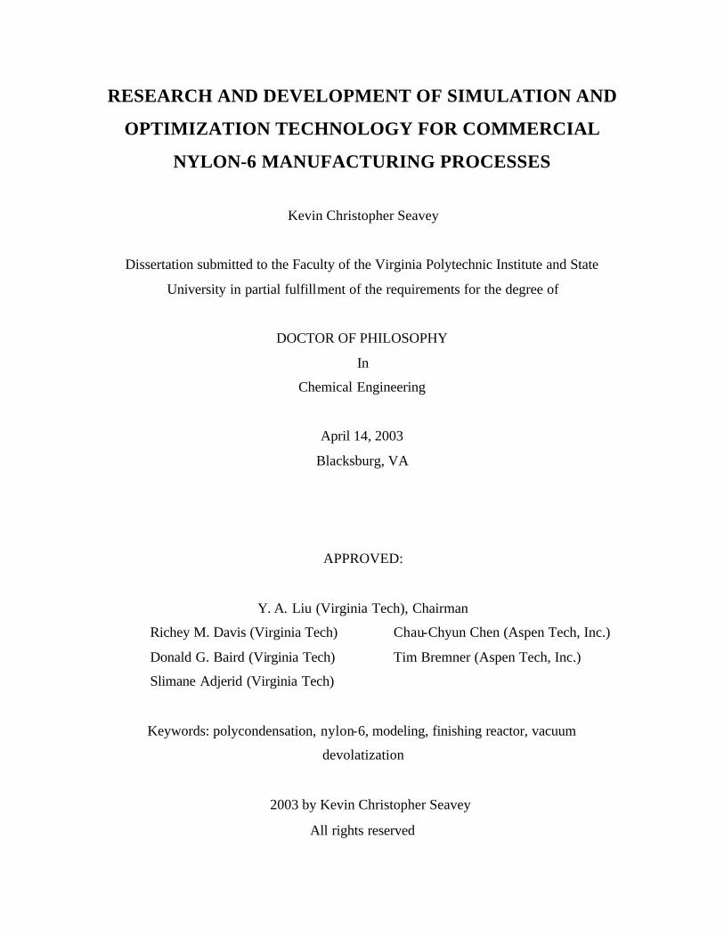
RESEARCH AND DEVELOPMENT OF SIMULATION AND
OPTIMIZATION TECHNOLOGY FOR COMMERCIAL
NYLON-6 MANUFACTURING PROCESSES
Kevin Christopher Seavey
Dissertation submitted to the Faculty of the Virginia Polytechnic Institute and State
University in partial fulfillment of the requirements for the degree of
DOCTOR OF PHILOSOPHY
In
Chemical Engineering
April 14, 2003
Blacksburg, VA
APPROVED:
Y. A. Liu (Virginia Tech), Chairman
Richey M. Davis (Virginia Tech) Chau-Chyun Chen (Aspen Tech, Inc.)
Donald G. Baird (Virginia Tech) Tim Bremner (Aspen Tech, Inc.)
Slimane Adjerid (Virginia Tech)
Keywords: polycondensation, nylon-6, modeling, finishing reactor, vacuum
devolatization
2003 by Kevin Christopher Seavey
All rights reserved
ii
Research and Development of Simulation and Optimization Technology for
Commercial Nylon-6 Manufacturing Processes
Kevin C. Seavey
Abstract
This dissertation concerns the development of simulation and optimization technology for
industrial, hydrolytic nylon-6 polymerizations. The significance of this work is that it is a
comprehensive and fundamental analysis of nearly all of the pertinent aspects of
simulation. It steps through all of the major steps for developing process models,
including simulation of the reaction kinetics, phase equilibrium, physical properties, and
mass-transfer- limited devolatization. Using this work, we can build accurate models for
all major processing equipment involved in nylon-6 production.
Contributions in this dissertation are of two types. Type one concerns the formalization
of existing knowledge of nylon-6 polymerization mixtures, mainly for documentation and
teaching purposes. Type two, on the other hand, concerns original research contributions.
Formalizations of existing knowledge include reaction kinetics and physical properties.
Original research contributions include models for phase equilibrium, diffusivities of
water and caprolactam, and devolatization in vacuum-finishing reactors.
We have designed all of the models herein to be fundamental, yet accessible to the
practicing engineer. All of the analysis was done using commercial software packages
offered by Aspen Technology, Cambridge, MA. We chose these packages for two
reasons: (1) These packages enable one to quickly build fundamental steady-state and
dynamic models of polymer trains; and (2) These packages are the only ones
commercially available for simulating polymer trains.
iii
Acknowledgements
First and foremost, I thank my advisor, Professor Y. A. Liu, for giving me the
opportunity to be a member in his research group. In addition to giving me a challenging
research topic, he has provided countless opportunities to meet practicing engineers from
across the globe and work with them to improve their processes. He has also provided
me with opportunities to work closely with Aspen Tech’s polymer simulation group,
which allowed me to learn world-class, state-of-the-art simulation technology for
industrial polymerization processes.
I also thank my committee members for the time and effort that they have invested into
my professional development. Specifically, I thank Professors Donald G. Baird and
Richey M. Davis for teaching me engineering rheology. I thank Professor Slimane
Adjerid and Donald G. Baird for teaching me numerical analysis and implementation. I
thank Chau-Chyun Chen for teaching me equilibrium thermodynamics for process
design. Lastly, I thank Tim Bremner for teaching me the finer aspects of polymer
chemistry and rheology, and for teaching me scientific skepticism. Tim always keeps my
mind in check when it wanders beyond the bounds of the data. He has also provided
much rheological data and shared with me many valuable insights about the chemical
process industries.
I also thank my fellow group members. Neeraj P. Khare has not only been a colleague of
the highest measure, but is also a friend. We have had countless productive discussions
in the office as well as memorable experiences traveling to conferences and
manufacturing sites. I also thank Bruce Lucas for more great experiences and interesting
discussions regarding the solid-state polymerization of step-growth polymers. Lastly, I
thank Richard Oldland for asking many questions and for seeking guidance from me – I

iv
hope that the little that I have passed on will serve him well. The cohesion of the group
has been a great advantage for helping us struggle, cope, and grow in the graduate school
environment.
I also thank Aspen Tech’s step-growth polymerization expert, David Tremblay. He has
taught me everything I know about simulating nylon-6 polymerizations, from reaction
kinetics to simulating mass-transfer-limited devolatization using penetration theory. I
also thank the many personnel of Honeywell, Inc., for giving me the chance to work on
their nylon-6 processes. These people include Thomas N. Williams, Earl Schoenborn,
John Mattson, Charlie Larkin, and Steve Davies. Seeing the processing equipment and
looking into operating vessels has helped me significantly, giving me new ideas for
simulating nylon-6 polymerization systems.
I also thank all of the undergraduate assistants that I have had the pleasure to work with.
Eva J. Shaw (now Wagner), Tom Lee, Jason Pettrey, Kristen Koch, Farzana Ahmed, and
Amber Wawro have done much great work and have added an element of charm and
liveliness to our offices.
I also express my gratitude and thanks to my parents, Robert S. Seavey and Yasuko
Seavey. They have, through their many years of hard work and patience, selflessly given
me the opportunity to pursue a higher education. Without their foresight and charity, I
would not be where I am today.
Finally, I thank Honeywell, Inc., SINOPEC, China Petrochemical Corporation, Aspen
Technology, and AlliantTechsystems for financial support and for giving me the
opportunity to work on many challenging, industrial problems. They continually teach
the great gift called pragmatism – it remains a valuable guide to lifelong, on-the-job
education.

v
Table of Contents
ABSTRACT ................................................................................................................................................................... II
ACKNOWLEDGEMENTS ..................................................................................................................................... III
TABLE OF CONTENTS ............................................................................................................................................ V
LIST OF FIGURES ..................................................................................................................................................... X
LIST OF TABLES ....................................................................................................................................................XIV
1 INTRODUCTION AND DIS SERTATION SCOPE/ORGANIZATION............................................1
1.1 INTRODUCTION TO CHEMICAL ENGINEERING AND PROCESS SIMULATION........................................ 2 1.2 INTRODUCTION TO POLYMER CHEMISTRY.............................................................................................. 3 1.3 DISSERTATION SCOPE AND ORGANIZATION............................................................................................ 6
2 REACTION KINETICS OF NYLON-6 .......................................................................................................9
2.1 INTRODUCTION.......................................................................................................................................... 10 2.2 SPECIES IDENTIFICATION AND FUNCTIONAL GROUP DEFINITION..................................................... 10 2.3 REACTIONS AND KINETICS ...................................................................................................................... 19
2.3.1 Ring Opening of Caprolactam..........................................................................................................22 2.3.2 Polycondensation................................................................................................................................23 2.3.3 Polyaddition of Caprolactam............................................................................................................26 2.3.4 Ring Opening of Cyclic Dimer..........................................................................................................27 2.3.5 Polyaddition of Cyclic Dimer............................................................................................................27 2.3.6 Monofunctional Acid Condensation.................................................................................................28 2.3.7 Monofunctional Amine Caprolactam Addition..............................................................................29 2.3.8 Monofunctional Amine Polycondensation......................................................................................30 2.3.9 Concentration of Terminated and Unterminated Linear Monomers and Dimers ...................31 2.3.10 Reaction and Rate Summary........................................................................................................34
2.4 SPECIES BALANCE..................................................................................................................................... 37 2.5 POLYMER PROPERTIES.............................................................................................................................. 38 2.6 BATCH REACTOR SIMULATION............................................................................................................... 42 2.7 CONCLUSIONS............................................................................................................................................ 46 2.8 NOMENCLATURE ....................................................................................................................................... 48 2.9 APPENDIX – FORTRAN 77 CODE FOR NYLON-6 BATCH REACTOR SIMULATION (DIGITAL
VISUAL FORTRAN 6.0) .......................................................................................................................................... 49
vi
3 PHASE EQUILIBRIUM IN NYLON-6 POLYMERIZATIONS ........................................................53
3.1 INTRODUCTION.......................................................................................................................................... 54 3.1.1 Commercial Nylon-6 Manufacturing Processes............................................................................54 3.1.2 Previous Nylon-6 Simulation Research...........................................................................................57 3.1.3 Objectives of Current Study ..............................................................................................................59
3.2 LITERATURE REVIEW................................................................................................................................ 61 3.2.1 Nylon-6 Polymerization Kinetics......................................................................................................61 3.2.2 Polymer Equilibrium..........................................................................................................................63
3.2.2.1 Previous Attempts to Develop a Phase-Equilibrium Model for Water/Caprolactam/Nylon-6 ... 63 3.2.2.2 POLYNRTL Model..................................................................................................................... 65
3.2.3 Equilibrium Data for Water/Caprolactam/Nylon-6......................................................................67 3.3 METHODOLOGY......................................................................................................................................... 67
3.3.1 Characterizing the Phase Equilibrium of Water/Caprolactam...................................................67 3.3.1.1 Consistency Test One: Van Ness et al. Test................................................................................ 68 3.3.1.2 Consistency Test Two: Wisniak Test.......................................................................................... 70 3.3.1.3 Determining Binary Interaction Parameters from Phase-Equilibrium Data................................ 71
3.3.2 Characterizing the Ternary, Reactive System Water/Caprolactam/Nylon-6............................72 3.4 RESULTS AND DISCUSSION ...................................................................................................................... 73
3.4.1 Binary Interaction Parameters for Water/Caprolactam..............................................................73 3.4.2 Binary Interaction Parameters for Water/Caprolactam/Nylon-6...............................................80
3.5 VALIDATION OF REGRESSED BINARY INTERACTION PARAMETERS.................................................. 83 3.6 MODEL APPLICATION............................................................................................................................... 86
3.6.1 Melt Train Model ................................................................................................................................87 3.6.2 Bubble-Gas Kettle Train Model........................................................................................................92 3.6.3 Example Summary...............................................................................................................................94
3.7 CONCLUSIONS............................................................................................................................................ 94 3.8 NOMENCLATURE ....................................................................................................................................... 96 3.9 SUPPORTING INFORMATION..................................................................................................................... 98
4 PHYSICAL PROPERTIES OF NYLON-6 POLYMERIZATION SYSTEMS ........................... 101
4.1 INTRODUCTION TO NYLON-6 POLYMERIZATION................................................................................102 4.2 PURE-COMPONENT PHYSICAL PROPERTIES FOR NYLON-6 POLYMERIZATION..............................104
4.2.1 Molecular Weight............................................................................................................................. 104 4.2.2 Critical Constants............................................................................................................................ 105 4.2.3 Vapor Pressure................................................................................................................................. 106 4.2.4 Vapor Molar Volume....................................................................................................................... 107 4.2.5 Liquid Molar Volume ...................................................................................................................... 108 4.2.6 Ideal Gas Enthalpy.......................................................................................................................... 110

vii
4.2.7 Ideal Liquid Enthalpy...................................................................................................................... 112 4.2.8 Polymer Rheology............................................................................................................................ 116
4.3 MIXTURE PROPERTIES FOR NYLON-6 POLYMERIZATION..................................................................122 4.3.1 Vapor Molar Volume....................................................................................................................... 122 4.3.2 Liquid Molar Volume ...................................................................................................................... 122 4.3.3 Vapor Mixture Enthalpy.................................................................................................................. 122 4.3.4 Liquid Mixture Enthalpy................................................................................................................. 123
4.4 VAPOR-LIQUID EQUILIBRIUM FOR NYLON-6 POLYMERIZATION.....................................................123 4.5 FORTRAN 77 IMPLEMENTATION ........................................................................................................124
4.5.1 Purpose of the Code......................................................................................................................... 124 4.5.2 Molecular Weight (Subroutine MOLECULARWEIGHT) ......................................................... 127 4.5.3 Vapor Pressure (Subroutines VAPORPRESSURE and ANTOINE) ........................................ 127 4.5.4 Critical Constants (Subroutine CRITICALPROPS)................................................................... 129 4.5.5 Vapor Molar Volume, Fugacity Coefficients, and Enthalpy Departure (Subroutine
FUGACITY) ...................................................................................................................................................... 130 4.5.6 Binary Interaction Parameters (Subroutine BINARY) .............................................................. 130 4.5.7 Activity Coefficients (Subroutine ACTIVITY).............................................................................. 131 4.5.8 Liquid Molar Volume Parameters (Subroutine MOLVOLP) ................................................... 134 4.5.9 Pure-Component Liquid Molar Volume (Subroutine LIQUIDMOLARVOLUME) .............. 135 4.5.10 Pure-Component Enthalpy Parameters (Subroutine ENTHPARAM) ............................... 136 4.5.11 Mixture Vapor Enthalpy (Subroutine VAPORENTHALPY)................................................ 138 4.5.12 Mixture Liquid Enthalpy (Subroutine LIQUIDENTHALPY) .............................................. 139 4.5.13 Poynting Correction (Subroutine POYNTING) ..................................................................... 142 4.5.14 Normalization of Composition Variables (Subroutine NORMALIZE) .............................. 142 4.5.15 Mole-to-Mass and Mass-to-Mole Conversions (Subroutines MOLETOMASS and
MASSTOMOLE) ............................................................................................................................................... 143 4.5.16 Dew Pressure Computation (Subroutine DEWPRESSURE) ............................................... 144 4.5.17 Bubble Pressure Computation (Subroutine BUBBLEPRESSURE) ................................... 146 4.5.18 TP-VLE Flash (Subroutine FLASH)........................................................................................ 148 4.5.19 Driver Program (Program STREAMFLASH)........................................................................ 153
4.6 PERFORMANCE OF SIMULATION............................................................................................................154 4.7 CONCLUSIONS..........................................................................................................................................155 4.8 NOMENCLATURE .....................................................................................................................................156 4.9 APPENDIX - FORTRAN 77 CODE (DIGITAL VISUAL FORTRAN 6.0) ........................................158
5 A MODEL FOR THE DIFFUSIVITY OF WATER AND CAPROLACTAM IN
CONCENTRATED NYLON-6 SOLUTIONS .................................................................................................. 179
5.1 INTRODUCTION........................................................................................................................................180

viii
5.2 SIMULATION PROBLEM...........................................................................................................................181 5.3 THEORETICAL ..........................................................................................................................................184
5.3.1 Mass-Transfer Theory ..................................................................................................................... 184 5.3.2 Modeling the Diffusivity of Volatile Species in Concentrated Polymer Solutions................ 187
5.3.2.1 Specific Hole Free Volume and Overlap Factor........................................................................ 190 5.3.2.2 Pre-exponential Factor............................................................................................................... 190 5.3.2.3 Ratio of Molar Volume of Jumping Units................................................................................. 191
5.3.3 Reaction Kinetics.............................................................................................................................. 192 5.4 IMPLEMENTATION ...................................................................................................................................197 5.5 RESULTS AND DISCUSSION ....................................................................................................................198
5.5.1 Estimates of Free-Volume Parameters......................................................................................... 198 5.5.2 Batch Reaction/Diffusion Results.................................................................................................. 207
5.6 APPLICATION OF DIFFUSIVITY MODEL................................................................................................215 5.7 CONCLUSIONS..........................................................................................................................................219 5.8 NOMENCLATURE .....................................................................................................................................221
6 SIMULATION OF VACUUM REACTORS FOR FINISHING STEP-GROWTH POLYMERS
223
6.1 INTRODUCTION TO THE COMMERCIAL PRODUCTION OF STEP -GROWTH POLYMERS....................224 6.1.1 Batch and Continuous Polymer Trains........................................................................................ 224
6.2 FINISHING REACTOR TECHNOLOGY .....................................................................................................227 6.3 ANALYSIS OF THE DESIGN AND OPERATION OF FINISHING REACTORS ..........................................231
6.3.1 Initial Steps towards Understanding Finishing Reactors......................................................... 232 6.3.2 Current Modeling Approach for Industrial Finishing Reactors.............................................. 235 6.3.3 Modern Analysis of Bubble-Gas Kettles...................................................................................... 237 6.3.4 Modern Analysis of Rotating-Disk Reactors............................................................................... 239 6.3.5 Literature Review Summary........................................................................................................... 241
6.4 THEORETICAL ..........................................................................................................................................244 6.4.1 Mass Transfer due to Bubbling...................................................................................................... 245 6.4.2 Mass Transfer due to Diffusion ..................................................................................................... 249
6.4.2.1 Penetration Theory..................................................................................................................... 250 6.4.2.2 Estimating the Interfacial Surface Area and Renewal Time ..................................................... 252
6.4.3 Reaction Kinetics.............................................................................................................................. 254 6.5 IMPLEMENTATION ...................................................................................................................................259 6.6 MODEL PERFORMANCE AND VALIDATION..........................................................................................261
6.6.1 Using Diffusion to Model the Finishing Reactors...................................................................... 261 6.6.2 Using Diffusion and Bubbling to Model the Finishing Reactors............................................. 267
6.7 CONCLUSIONS..........................................................................................................................................272

ix
6.8 NOMENCLATURE .....................................................................................................................................275
7 CONCLUSIONS AND FUTURE WORK............................................................................................... 277
7.1 HEAT TRANSFER......................................................................................................................................277 7.2 MASS-TRANSFER-LIMITED DEVOLATIZATION ...................................................................................277
VITA............................................................................................................................................................................. 280

x
List of Figures
FIGURE 1.1. CHEMICAL FORMULA FOR POLYETHYLENE – THE BRACKETS DENOTE A REPEAT UNIT, REPEATED
N TIMES AND COVALENTLY BONDED END-TO-END AS SHOWN FOR THE OTHER REPEAT UNITS.................. 3 FIGURE 1.2. FREE-RADICAL ADDITION OF ETHYLENE TO FORM POLYETHYLENE................................................... 4 FIGURE 1.3. TWO NYLON-6 CHAINS, OF DEGREE OF POLYMERIZATION N AND M, REACT TO FORM ONE LONGER
CHAIN OF DEGREE OF POLYMERIZATION N+M. WATER IS THE SMALL MOLECULE THAT IS ELIMINATED.5 FIGURE 1.4. CAPROLACTAM CONVERSION REACTIONS IN THE HYDROLYTIC POLYMERIZATION OF NYLON-6... 6 FIGURE 2.1. NON-POLYMERIC SPECIES INVOLVED IN HYDROLYTIC POLYMERIZATION OF NYLON 6................. 12 FIGURE 2.2. A FIVE-SEGMENT , LINEAR POLYMER CHAIN CONSISTING OF TWO TERMINAL SEGMENTS AND
THREE BOUND SEGMENTS................................................................................................................................... 13 FIGURE 2.3. POLYMERIC SPECIES WITH A DEGREE OF POLYMERIZATION OF ONE ................................................ 15 FIGURE 2.4. POLYMERIC SPECIES OF DEGREE OF POLYMERIZATION TWO............................................................. 17 FIGURE 2.5. POLYMERIC SPECIES OF LENGTH N, WHERE N GOES FROM THREE TO INFINITY............................... 18 FIGURE 2.6. RING OPENING OF CAPROLACTAM VIA WATER.................................................................................... 22 FIGURE 2.7. POLYCONDENSATION EQUILIBRIUM REACTION. THE GROUP R CAN STAND FOR HYDROGEN, A
HYDROXYL GROUP, OR A TERMINATOR GROUP................................................................................................ 23 FIGURE 2.8. ADDITION OF CAPROLACT AM................................................................................................................. 26 FIGURE 2.9. RING-OPENING OF CYCLIC DIMER.......................................................................................................... 27 FIGURE 2.10. POLYADDITION OF CYCLIC DIMER....................................................................................................... 28 FIGURE 2.11. MONOFUNCTIONAL ACID TERMINATION ............................................................................................ 29 FIGURE 2.12. ADDITION OF CAPROLACT AM VIA MONOFUNCTIONAL AMINE ........................................................ 30 FIGURE 2.13. MONOFUNCTIONAL AMINE POLYCONDENSATION WITH A POLYMERIC CARBOXYL GROUP ........ 30 FIGURE 2.14. AMINE END GROUP CONCENTRATION AND POLYMER MASS AS A FUNCTION OF TIME IN A BATCH
REACTOR (INITIAL CHARGE IS 1 KG WATER, 99 KG CAPROLACTAM)............................................................ 43 FIGURE 2.15. CYCLIC DIMER AND POLYMER PRODUCTION VS. TIME IN A LIQUID-ONLY BATCH REACTOR
(INITIAL CHARGE IS 1 KG WATER, 99 KG CAPROLACTAM). ............................................................................ 44 FIGURE 2.16. ADDITION OF ACETIC ACID INCREASES THE RATE OF POLYMERIZATION VIA INCREASE IN
CARBOXYLIC ACID FUNCTIONALITIES (INITIAL CHARGE IS 1 KG WATER, 99 KG CAPROLACTAM, AND 0.21
KG ACETIC ACID).................................................................................................................................................. 45 FIGURE 2.17. ACETIC ACID/CYCLOHEXYLAMINE TERM INATED NYLON 6 BATCH POLYMERIZATION (INITIAL
CHARGE IS 1 KG WATER, 99 KG CAPROLACTAM, 0.21 KG ACETIC ACID, AND 0.35 KG
CYCLOHEXYLAMINE)........................................................................................................................................... 46 FIGURE 3.1. A BLOCK DIAGRAM OF A CONVENTIONAL NYLON-6 POLYMERIZATION PROCESS............................. 55 FIGURE 3.2. DEVELOPING A MODEL FOR THE BINARY INTERACTIONS WITHIN THE TERNARY SYSTEM
WATER/CAPROLACTAM/NYLON-6...................................................................................................................... 60
xi
FIGURE 3.3. PERCENT ERROR IN VAPOR MOLE FRACTION PREDICTION VS. LIQUID MOLE FRACTION FOR
CAPROLACTAM FOR ALL DATA SETS (VAN NESS ET AL. TEST )...................................................................... 74 FIGURE 3.4. L/W RATIO VS. CAPROLACTAM LIQUID MOLE FRACTION FOR ALL DATA SETS (WISNIAK TEST ).. 75 FIGURE 3.5. PREDICTED VALUE OF THE POLYNRTL BINARY PARAMETER TAU FOR WATER/CAPROLACTAM
AND CAPROLACTAM/WATER............................................................................................................................... 76 FIGURE 3.6. WATER/CAPROLACTAM T-X-Y DIAGRAM (101,325 PA)...................................................................... 77 FIGURE 3.7. WATER/CAPROLACTAM T-X-Y DIAGRAM (24,000 PA). ....................................................................... 78 FIGURE 3.8. WATER/CAPROLACTAM T-X-Y DIAGRAM (10,700 PA). ....................................................................... 79 FIGURE 3.9. WATER/CAPROLACTAM T-X-Y DIAGRAM (4,000 PA). ......................................................................... 80 FIGURE 3.10. MASS FLOW RATES EXITING CONDENSER - MODEL PREDICTION VS. PLANT EXPERIENCE. ALL
VALUES HAVE BEEN NORMALIZED USING THE LARGEST FLOW RATE........................................................... 84 FIGURE 3.11. FOUR-REACTOR NYLON-6 MANUFACTURING PROCE SS. MOST OF THE MONOMER CONVERSION
TAKES PLACE IN THE FIRST TWO REACTORS, WHILE THE MOLECULAR WEIGHT BUILD OCCURS IN THE
THIRD AND FOURTH REACTORS. THE SECOND VESSEL HAS A REFLUX CONDENSER WHILE THE ENTIRE
TRAIN HAS A CONDENSER TO RECYCLE THE UNREACTED MONOMER........................................................... 88 FIGURE 3.12. THREE-REACTOR NYLON-6 MANUFACTURING PROCESS. LACTAM AND WATER ARE FED TO THE
FIRST MULTI-PHASE KETTLE, WHILE INERT GAS FLOW DEVOLATILIZES THE SECOND AND THIRD
VESSELS. ................................................................................................................................................................ 92 FIGURE 4.1. NON-POLYMERIC SPECIES PRESENT IN NYLON-6 POLYMERIZATION MIXTURES............................102 FIGURE 4.2. POSSIBLE STRUCTURES OF NYLON-6: THE NYLON-6 REPEAT UNIT IS B-ACA (TWO COVALENT
BONDS TO THE REST OF THE POLYMER MOLECULE). POSSIBLE ENDGROUPS ARE T-COOH OR T-CHA
AND T-NH2 OR T-HOAC (ONE COVALENT BOND TO THE REST OF THE POLYMER MOLECULE). ...........103 FIGURE 4.3. IDEAL GAS VAPOR MOLAR VOLUME PREDICTIONS FOR WATER (DATA FROM SANDLER) ............108 FIGURE 4.4. TAIT MOLAR VOLUME PREDICTIONS FOR NYLON-6 COMP ARED TO EXPERIMENTAL DATA.........110 FIGURE 4.5. HEAT CAPACITY OF MOLTEN NYLON-6...............................................................................................114 FIGURE 4.6. REGRESSED ENTHALPY OF NYLON-6 AT 313 K..................................................................................115 FIGURE 4.7. NON-NEWTONIAN SHEAR VISCOSITY OF NYLON-6 (NUMBER-AVERAGE MOLECULAR WEIGHT OF
22,500 G/MOL)....................................................................................................................................................117 FIGURE 4.8. FLOW CURVES AT 250 AND 270 °C PREDICTED USING TEMPERATURE SHIFT FACTOR.................120 FIGURE 4.9. STREAM VECTOR CONTAINING STREAM CONDITIONS AND FLOW RATES FOR EACH SPECIES 1
THROUGH N. THE STREAM VECTOR ALSO CONTAINS THE DEGREE OF POLYMERIZATION FOR EACH
SPECIES................................................................................................................................................................125 FIGURE 5.1. BATCH DIFFUSION/REACTION APPARATUS OF NAGASUBRAMANIAN AND REIMSCHUESSEL ......182 FIGURE 5.2. PENETRATION THEORY REPRESENTATION OF THE CONCENTRATION GRADIENT IN THE DIFFUSION
OF A SPECIES THROUGH THE LIQUID PHASE INTO THE VAPOR PHASE – CL IS THE BULK-PHASE
CONCENTRATION WHILE CL* IS THE LIQUID-PHASE INTERFACIAL CONCENTRATION...............................185
xii
FIGURE 5.3. A MOLECULAR LATTICE THAT HAS HOLES BETWEEN THE MOLECULES. FOR A MOLECULE TO
MOVE, A VOID VOLUME AT LEAST AS LARGE AS THE SPECIFIC HOLE VOLUME MUST BE PRESENT .........188 FIGURE 5.4. VOGEL EQUATION (EQ. (5.10)) FIT TO VISCOSITY DATA FOR WATER AND CAP ROLACTAM........200 FIGURE 5.5. NORMALIZED VOGEL PARAMETERS (EQ. (5.10)) AS A FUNCTION OF NYLON-6 MOLECULAR
WEIGHT ................................................................................................................................................................201 FIGURE 5.6. PRE-EXPONENTIAL FACTOR FOR VRENTAS-DUDA FREE-VOLUME EQUATION (FOR WATER,
GENERATED USING EQS. (5.11) AND (5.12)) ..................................................................................................204 FIGURE 5.7. PRE-EXPONENTIAL FACTOR FOR VRENTAS-DUDA FREE-VOLUME EQUATION (FOR
CAPROLACTAM, GENERATED USING EQS. (5.11) AND (5.12)) .....................................................................205 FIGURE 5.8. PENETRATION-THEORY MODEL USING RIGOROUS BOUNDARY CONDITIONS AND THE DIFFUSION
CONSTANTS OF NAGASUBRAMANIAN AND REIMSCHUESSEL ......................................................................208 FIGURE 5.9. VRENTAS-DUDA FREE-VOLUME MODEL FOR DIFFUSION COEFFICIENT ALONG WITH PENET RATION
THEORY AND EQUILIBRIUM BOUNDARY CONDITIONS (VRENTAS-DUDA PARAMETERS REGRESSED FROM
VISCOSITY AND DENSIT Y DATA ONLY)............................................................................................................210 FIGURE 5.10. VRENTAS-DUDA FREE-VOLUME MODEL FOR DIFFUSION COEFFICIENT ALONG WITH
PENETRATION THEORY AND EQUILIBRIUM BOUNDARY CONDITIONS (VRENTAS-DUDA ADJUSTED TO FIT
DIFFUSION DATA)...............................................................................................................................................212 FIGURE 5.11. BATCH REACTOR PROFILE FOR ACCUMULATED MASS....................................................................216 FIGURE 5.12. COMPARISON OF NORMALIZED CAPROLACTAM WEIGHT FRACTION (CL) AND FORMIC-ACID
VISCOSITY (FAV) PROFILES (CL INITIAL VALUE 0.0815, FAV INITIAL VALUE 16.7) – CAPROLACTAM
DEVOLATIZATION IS HARDLY AFFECTED BY SURFACE RENEWAL EVERY MINUTE CAUSED BY MIXING
WHEREAS INCREASED WATER EVAPORATION CAUSES THE FAV TO RISE MODESTLY..............................218 FIGURE 5.13. COMPARISON OF NORMALIZED CAPROLACTAM WEIGHT FRACTION (CL) AND FORMIC-ACID
VISCOSITY (FAV) PROFILES (CL INITIAL VALUE 0.0815, FAV INITIAL VALUE 16.7) – CASE ONE:
MIXING AND 2.5X SURFACE AREA AND CASE TWO: MIXING AND VACUUM OF 50 MM HG......................219 FIGURE 6.1. NYLON-6 PRODUCTION TRAIN (BUBBLE-GAS TYPE) WITH THREE POLYMERIZATION REACTORS
AND POST -POLYMERIZATION UNITS – THE FIRST REACTOR CARRIES OUT MONOMER CONVERSION, WHILE
THE SECOND AND THIRD REACTORS BUILD UP THE MOLECULAR WEIGHT OF THE POLYMER BY WATER
REMOVAL............................................................................................................................................................224 FIGURE 6.2. FOUR-REACTOR NYLON-6 MELT TRAIN – THE FIRST TWO REACT ORS PERFORM MONOMER
CONVERSION, WHILE THE SECOND TWO REACTORS PERFORM P OLYMER DEVOLATIZATION AND
MOLECULAR-WEIGHT BUILD.............................................................................................................................226 FIGURE 6.3. BUBBLE-GAS KETTLE FOR FINISHING STEP -GROWTH POLYMER MELTS.........................................227 FIGURE 6.4. BATCH REACTION SCHEME FOR MANUFACTURING NYLON-6 ..........................................................228 FIGURE 6.5. WIPED-WALL EVAPORATOR – WIPERS MOUNTED ON A ROTATING SHAFT APPLY THE
PREPOLYMER AS A FILM ON THE REACTOR WALLS TO MAXIMIZE INTERFACIAL SURFACE AREA...........230 FIGURE 6.6. ROTATING-DISK FINISHING REACT OR.................................................................................................231
xiii
FIGURE 6.7. INITIAL APPROACH FOR MODELING THIN-FILM FINISHING REACT ORS............................................233 FIGURE 6.8. DIFFUSION OF VOLATILE SPECIES INTO THE BULK VAPOR PHASE AND INTO BUBBLES DISPERSED
IN THE POLYMER MELT......................................................................................................................................234 FIGURE 6.9. CONCENTRATION PROFILE VS. DISTANCE IN A DEVOLATIZING SLAB OF POLYMER SOLUTION...236 FIGURE 6.10. COMPARTMENTAL MODELING STRATEGY FOR THE ROTATING-DISK REACTOR..........................240 FIGURE 6.11. DEPICTION OF PRESSURES INSIDE AND OUTSIDE THE BUBBLE, AND THE FORCE OF SURFACE
TENSION. THE EQUATION IS THE CONDITION FOR MECHANICAL EQUILIBRIUM, WITH R BEING THE
BUBBLE RADIUS..................................................................................................................................................246 FIGURE 6.12. PENETRATION THEORY ANALYSIS OF INDUSTRIAL-SCALE UNIT OPERATIONS WITH AGITATION
..............................................................................................................................................................................250 FIGURE 6.13. CROSS-SECTION OF ROTATING DISK REACTOR DEPICTING THE LIQUID LEVEL AND THE
SUBSEQUENT ANGLE THETA THAT IS FORMED ...............................................................................................253 FIGURE 6.14. SIMULATION FLOW SHEET FOR A CONTINUOUS NYLON-6 POLYMERIZATION PROCESS .............260 FIGURE 6.15. DIFFUSION COEFFICIENT OF WATER IN THE WIPED-WALL EVAPORATOR AND ROTATING-DISK
REACTOR.............................................................................................................................................................263 FIGURE 6.16. DIFFUSION COEFFICIENT OF CAPROLACTAM IN T HE WIPED-WALL EVAPORATOR AND ROTATING-
DISK REACTOR....................................................................................................................................................264 FIGURE 6.17. KEY POLYMER CHARACTERISTIC AS A FUNCTION OF PRODUCTION RATE...................................267

xiv
List of Tables
TABLE 2.1. CHEMICAL FORMULAS FOR NON-POLYMERIC SPECIES......................................................................... 12 TABLE 2.2. CHEMICAL FORMULAS FOR POLYMERIC SPECIES.................................................................................. 14 TABLE 2.3. FUNCTIONAL GROUP MOLECULAR WEIGHTS......................................................................................... 18 TABLE 2.4. SUMMARY OF EQUILIBRIUM REACTIONS AND ACCOMPANYING REACTION RATES.......................... 34 TABLE 2.5. RATE CONSTANTS FOR THE ARAI ET AL.* EQUILIBRIUM SCHEME....................................................... 37 TABLE 2.6. DIFFERENTIAL EQUATIONS DESCRIBING THE TIME RATE OF CHANGE FOR ALL FUNCTIONAL
GROUPS. THESE EQUATIONS ALSO DOUBLE AS A SIMULATION FOR LIQUID-PHASE-ONLY BATCH
REACTORS. ............................................................................................................................................................ 37 TABLE 3.1. NYLON-6 PRODUCTION/RECYCLING TECHNOLOGIES PRACTICED ON A COMMERCIAL SCALE........ 57 TABLE 3.2. NYLON-6 POLYMERIZATION REACTION MECHANISMS......................................................................... 61 TABLE 3.3. RATE CONSTANTS FOR THE EQUILIBRIUM REACTIONS IN TABLE 3.2................................................. 62 TABLE 3.4. LIQUID-PHASE, WATER MOLE-FRACTION PREDICTIONS AT ONE ATMOSPHERE FOR THE
JACOBS/SCHWEIGMAN, FUKUMOTO, AND TAI ET AL. PHASE-EQUILIBRIUM MODELS................................ 65 TABLE 3.5. PHYSICAL PROPERTY CONSTANTS FOR WATER AND CAPROLACTAM. THE VAPOR PRESSURE IS
COMPUTED USING EQ. (3.9), WITH UNITS OF PA AND TEMPERATURE UNITS OF K. THE ENTHALPY OF
VAPORIZATION IS COMPUTED USING EQ. (3.15), WITH UNITS OF J/KMOL AND TEMPERATURE UNITS OF
K............................................................................................................................................................................. 73 TABLE 3.6. REGRE SSION RESULTS FOR POLYNRTL BINARY INTERACTION PARAMETERS FOR
WATER/CAPROLACTAM (BASED ON T-P-X DATA ONLY)................................................................................. 76 TABLE 3.7. COMPARISON OF MODEL P REDICTIONS WITH GIORI AND HAYES POLYMERIZATION DATA............ 81 TABLE 3.8. PREDICTIONS FOR LIQUID-PHASE WATER MOLE FRACTION OF PREVIOUS LITERATURE MODELS
AND THE IDEAL MODEL, AND COMPARISON WITH EXPERIMENTAL DATA.................................................... 82 TABLE 3.9. POLYNRTL BINARY INTERACTION PARAMETERS FOR WATER/CAPROLACTAM/NYLON-6
(TEMPERATURE UNITS ARE K)............................................................................................................................ 83 TABLE 3.10. OPERATING CONDITIONS FOR EACH UNIT OPERATION IN THE FOUR-VESSEL TRAIN...................... 90 TABLE 3.11. MODEL PREDICTIONS FOR LIQUID-PHASE MASS FLOW RATES EXITING EACH REACT OR............... 91 TABLE 3.12. OPERATING CONDITIONS FOR EACH KETTLE DEPICTED IN FIGURE 3.12. ALL OPERATING
CONDITIONS COME FROM REFERENCE 14. ........................................................................................................ 93 TABLE 3.13. PREDICTED LIQUID-STREAM COMPOSITIONS EXITING EACH KETTLE. ............................................. 93 TABLE 3.14. PHASE-EQUILIBRIUM DATA FOR THE SYSTEM WATER/CAPROLACTAM AT 101,325 PA
(MANCZINGER AND TETTAMANTI). .................................................................................................................. 98 TABLE 3.15. PHASE-EQUILIBRIUM DATA FOR T HE SYSTEM WATER/CAPROLACTAM AT 24,000 PA
(MANCZINGER AND TETTAMANTI). .................................................................................................................. 98
xv
TABLE 3.16. PHASE-EQUILIBRIUM DATA FOR THE SYSTEM WATER/CAPROLACTAM AT 10,700 PA
(MANCZINGER AND TETTAMANTI). .................................................................................................................. 99 TABLE 3.17. PHASE-EQUILIBRIUM DATA FOR THE SYSTEM WATER/CAPROLACTAM AT 4,000 PA
(MANCZINGER AND TETTAMANTI). .................................................................................................................. 99 TABLE 3.18. PHASE-EQUILIBRIUM DATA FOR THE SYSTEM WATER/CAPROLACTAM/NYLON-6 (GIORI AND
HAYES). GIORI AND HAYES USED A 0.020-KG CAPROLACTAM CHARGE FOR ALL POLYMERIZATIONS.
..............................................................................................................................................................................100 TABLE 4.1. CHEMICAL FORMULAS FOR NON-POLYMERIC SPECIES PRESENT IN NYLON-6 POLYMERIZATION
MIXTURES............................................................................................................................................................102 TABLE 4.2. CHEMICAL FORMULAS FOR POLYMER SEGMENTS...............................................................................104 TABLE 4.3. MOLECULAR WEIGHTS FOR NYLON-6 MIXTURES................................................................................105 TABLE 4.4. CRITICAL TEMPERATURE FOR THE SPECIES IN NYLON-6 POLYMERIZATION MIXTURES................105 TABLE 4.5. DIPPR VAPOR PRESSURE EQUATION PARAMETERS FOR NYLON-6 POLYMERIZATION MIXTURES.
VAPOR PRESSURE UNITS ARE PA AND TEMPERATURE UNITS ARE K...........................................................107 TABLE 4.6. DIPPR LIQUID MOLAR VOLUME PARAMETERS FOR NON-POLYMERIC SPECIES (MOLAR VOLUME IN
M3/KMOL AND TEMPERATURE IN K)................................................................................................................109 TABLE 4.7. IDEAL GAS ENTHALPY OF FORMATION .................................................................................................111 TABLE 4.8. DIPPR IDEAL GAS HEAT CAPACITY PARAMETERS (IDEAL GAS HEAT CAPACITY IN J/KMOL-K,
TEMPERATURE IN K, UPPER TEMPERATURE LIMIT IS 1,000 OR 1,500 K) ...................................................111 TABLE 4.9. DIPPR ENT HALPY OF VAPORIZATION PARAMETERS (ENTHALPY OF VAPORIZATION IN J/KMOL)112 TABLE 4.10. CARREAU-YASUDA EQUATION PARAMETERS FOR FLOW CURVES OF NYLON-6 AT VARIOUS
TEMPERATURES..................................................................................................................................................118 TABLE 4.11. MARK-HOUWINK CONSTANTS FOR NYLON-6 AT 25 °C ...................................................................121 TABLE 4.12. COMPUTATION SUBROUTINE INDEX ...................................................................................................125 TABLE 4.13. PHYSICAL PROPERTY CONSTANT SUBROUTINES INDEX...................................................................126 TABLE 4.14. EXAMPLE FLASH CALCULATION - PHYSICAL PROPERTY SYSTEM PREDICTIONS...........................154 TABLE 5.1. NYLON-6 POLYMERIZATION REACTION MECHANISMS (THIS STUDY DOES NOT INVOLVE
MONOFUNCTIONAL TERMINATOR SPECIES – THEREFORE , WE DO NOT CONSIDER THEM HERE)..............192 TABLE 5.2. RATE CONSTANTS FOR THE EQUILIBRIUM REACTIONS IN TABLE 5.1...............................................193 TABLE 5.3. COMPONENT/SEGMENT DEFINITIONS USED FOR SIMULATING NYLON-6 POLYMERIZATION USING
ASPEN TECH’S STEP -GROWTH POLYMERIZATION MODEL............................................................................194 TABLE 5.4. EQUILIBRIUM REACTIONS USING SEGMENT APPROACH.....................................................................195 TABLE 5.5. SPECIES CONSERVATION EQUATIONS FOR A LIQUID-ONLY, BATCH REACTION..............................196 TABLE 5.6. STARTING MATERIALS AND RESULTING POLYMER SOLUTION COMPOSITION.................................197 TABLE 5.7. VOGEL PARAMETERS FOR WATER, CAPROLACTAM, AND NYLON-6 .................................................202 TABLE 5.8. MOLECULAR WEIGHT AND CRITICAL MOLAR VOLUME FOR WATER AND CAPROLACTAM............202 TABLE 5.9. SPECIFIC VOLUME DIPPR PARAMETERS FOR WATER AND CAPROLACTAM....................................203
xvi
TABLE 5.10. FREE-VOLUME PARAMETERS FOR WATER, CAPROLACTAM, AND NYLON-6 REPEAT SEGMENT ( *iV
GENERATED USING EQ. (5.23) FOR WATER AND CAPROLACTAM; FOR NYLON-6, WE USED THE
CRYSTALLINE DENSITY)....................................................................................................................................206 TABLE 5.11. RATIO OF MOLAR VOLUME OF JUMPING UNITS.................................................................................207 TABLE 5.12. COMPARISON OF DIFFUSION COEFFICIENT VALUES ENCOUNTERED IN THIS STUDY (VALUES IN
PARENTHESIS ARE IN UNITS OF CM2/S).............................................................................................................213 TABLE 5.13. SUMMARY OF FREE-VOLUME PARAMETERS FOR EQS. (5.27), (5.29), AND (5.31) .......................214 TABLE 6.1. SUMMARY OF FREE-VOLUME PARAMETERS FOR EQS. (6.20), (6.22), AND (6.24)..........................252 TABLE 6.2. NYLON-6 POLYMERIZATION REACTION MECHANISMS.......................................................................254 TABLE 6.3. SEGMENT DEFINITIONS USED FOR SIMULATING NYLON-6 POLYMERIZATION.................................255 TABLE 6.4. EQUILIBRIUM REACTIONS USING SEGMENT APPROACH.....................................................................256 TABLE 6.5. SPECIES CONSERVATION EQUATIONS FOR A LIQUID-ONLY, BATCH REACTION..............................258 TABLE 6.6. OUTPUT VARIABLE PREDICTIONS USING ONLY DIFFUSIONAL-MASS TRANSFER THEORY.............262 TABLE 6.7. DEVOLATIZATION RATES OF FINISHING REACTORS CONSIDERING DIFFUSION AS THE SOLE
MECHANISM OF DEVOLATIZATION...................................................................................................................262 TABLE 6.8. DEVOLATIZATION RATES FOR THE WIPED-WALL EVAPORATOR AND ROTATING-DISK REACTOR –
BUBBLING MECHANISM VS. DIFFUSION MECHANISM (NUMBERS IN PARENTHESES ARE APPROXIMATE
PRODUCTION RATES) .........................................................................................................................................268

1
1 Introduction and Dissertation Scope/Organization
In this chapter, we introduce basic aspects of the engineering of polymer manufacturing
processes. We first introduce chemical process engineering and modeling. We then
review basic aspects of polymer chemistry and in particular, the commercial
manufacturing of nylon-6. Lastly, we give an outline of the dissertation.
Chapter organization is as follows:
• 1.1 – Introduction to chemical process simulation
• 1.2 – Introduction to polymer chemistry
• 1.3 – Overview of the scope and organization of the dissertation

2
1.1 Introduction to Chemical Engineering and Process
Simulation
The field of chemical engineering was established in the late nineteenth century by
George Davis of England and Lewis Norton of the Massachusetts Institute of
Technology1. It focused on the design and optimization of chemical manufacturing
processes. While modern chemical engineers (or more colloquially, chemE’s) can be
found in any technical field where a combined knowledge of mathematics, physics, and
chemistry is beneficial, many graduating chemE’s still find employment in the process
engineering departments of chemical manufacturing companies. These companies
manufacture pharmaceuticals, petrochemicals, polymers, and other chemicals.
Process engineers are interested in developing fundamental and/or empirical relationships
between key process inputs and outputs. For example, a reactor engineer may be
interested in the effect of reactor temperature on product characteristics. These
relationships between inputs and outputs constitute a model for the process. The model is
then used to optimize the process, i.e., investigate various operating alternatives in order
to find the most economical way to run the process. Models are also used for process
design and analysis of the controls and dynamics.
The later half of the twentieth century witnessed the start of the computer revolution.
Computing and communications technology has blossomed, allowing large amounts of
computations and data to be easily handled. With the proliferation of computing power,
process modeling has also changed. Complex, fundamental models are easily accessible
and commercially available. These models integrate knowledge of physical properties,
unit operations, and sometimes reaction kinetics in order to understand how reactors,
distillation columns, and other unit operations work. Process engineers then, armed with
this quantitative knowledge of how their processes work, use these models to improve
their processes by performing virtual experiments on their processes.
1 http://www.pafko.com/history/h_1888.html (accessed January 2004)

3
1.2 Introduction to Polymer Chemistry
This dissertation is concerned with the simulation and optimization of polymer
manufacturing processes – importantly, we focus on the hydrolytic polymerization
process for nylon-6. Therefore, we now review basic aspects of polymer chemistry for
those readers who are not familiar with the field.
Polymers, or macromolecules, are large molecules of considerable commercial
importance. They either occur naturally or are man-made. Natural polymers include
proteins and polysaccharides, while synthetic polymers include elastomers, thermoplastic
polymers, and thermosetting polymers2. Hemoglobin and cellulose are examples of
naturally occurring polymers, while polyethylene (PE) and nylon are examples of
synthetic polymers.
Individual polymer molecules are composed of repeating structural units, or segments.
Figure 1.1 shows the repeat nature of a linear polyethylene.
CH3
CH2CH2
CH2CH2
CH2CH2
CH2CH2
CH2CH2
CH2CH2
CH2CH2
CH3
n
Figure 1.1. Chemical formula for polyethylene – the brackets denote a repeat unit, repeated
n times and covalently bonded end-to-end as shown for the other repeat units
The number of repeat units in an individual polymer molecule is the degree of
polymerization DP. The molecular weight of a polymer molecule, neglecting end-groups,
is the DP multiplied by the repeat unit molecular weight. Polymer mixtures usually
contain molecules of different lengths, i.e., the molecular weight distribution is
polydisperse.
2 Cowie, J. M. G., Polymers: Chemistry & Physics of Modern Materials, 2nd ed., Blackie Academic and
Professional, New York, p. 3, 1991.

4
In 1929, Wallace Hume Carothers introduced a useful division among polymers: those
produced via a condensation process, and those produced via an addition process3.
Condensation, or step-growth, polymers are produced through a chemical reaction that
involves the elimination of a small molecule, whereas addition polymers are produced
with no such loss.
An example of an addition polymeriza tion is that of polyethylene by a free-radical
mechanism (Figure 1.2).
CH3 CH2
n+ CH2 CH2 CH3 CH2
n+1
Figure 1.2. Free-radical addition of ethylene to form polyethylene
Free-radical addition polymers are formed in three steps: initiation, propagation, and
termination. Radicals are formed in the initiation step, monomer is added to form a
growing polymer chain in the propagation step, and radicals are neutralized in the
termination step.
On the other hand, an example of a polycondensation, or molecular-weight build,
reaction is the growth of nylon-6, a polyamide (Figure 1.3).
3 Flory, P. J., Principles of Polymer Chemistry, Cornell University Press, Ithaca, New York, p. 37, 1953.
5
O
RNH
H+
n m
m+n
+ OH2
O
OHNH
R
O
RNH
R
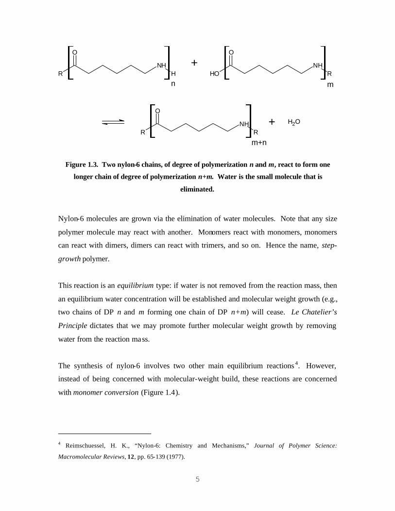
Figure 1.3. Two nylon-6 chains, of degree of polymerization n and m, react to form one
longer chain of degree of polymerization n+m. Water is the small molecule that is
eliminated.
Nylon-6 molecules are grown via the elimination of water molecules. Note that any size
polymer molecule may react with another. Monomers react with monomers, monomers
can react with dimers, dimers can react with trimers, and so on. Hence the name, step-
growth polymer.
This reaction is an equilibrium type: if water is not removed from the reaction mass, then
an equilibrium water concentration will be established and molecular weight growth (e.g.,
two chains of DP n and m forming one chain of DP n+m) will cease. Le Chatelier’s
Principle dictates that we may promote further molecular weight growth by removing
water from the reaction mass.
The synthesis of nylon-6 involves two other main equilibrium reactions 4. However,
instead of being concerned with molecular-weight build, these reactions are concerned
with monomer conversion (Figure 1.4).
4 Reimschuessel, H. K., “Nylon-6: Chemistry and Mechanisms,” Journal of Polymer Science:
Macromolecular Reviews, 12, pp. 65-139 (1977).

6
+ NH
O
n+1
O
RNH
H
n
O
RNH
H
NH
O
+ OH2
O
OHNH2
Figure 1.4. Caprolactam conversion reactions in the hydrolytic polymerization of nylon-6
The monomer for nylon-6 polymer is ε-caprolactam, the ring structure in Figure 1.4. In
the first conversion reaction, water opens the caprolactam ring to form aminocaproic
acid. In the second conversion reaction, an existing polymer chain directly adds a
caprolactam molecule to form a slightly larger polymer chain. The first equilibrium
reaction suggests that we must use high water concentrations in order to convert as much
caprolactam as possible into aminocaproic acid. We may think of aminocaproic acid as a
polymer molecule of DP one.
Commodity polymers, such as nylon-6, are typically produced in a low profit margin
regime. This being the case, these polymer processes must be designed and highly
optimized. Monomer must be converted rapidly into polymer, and the polymer must be
of sufficiently high molecular weight to have useful mechanical properties. Furthermore,
the finished polymer can only contain a trace amount of impurities, such as reaction by-
products and residual monomer.
1.3 Dissertation Scope and Organization
This dissertation is concerned with the research and development of simulation and
optimization technology for commercial nylon-6 manufacturing processes. This means
two things:
• Documentating existing simulation technology for nylon-6 polymerization
processes
7
• Identifying gaps in our knowledge and filling these gaps by creating new models.
In this case, we create new models of nylon-6 physical properties and vacuum-
finishing nylon-6.
The state of the literature regarding nylon-6 polymerization now follows. The kinetics of
polymerization are well-grounded. However, it is peculiar to note that the method-of-
moments is applied to simulating nylon-6 polymerization, yet a segment-based approach
is used to simulate poly(ethylene terephthalate) polymerization. We prefer the segment-
based approach because it is easier to apply to industrial polymerizations that utilize
multiple terminating species. Furthermore, moments of the molecular-weight distribution
such as the weight-average molecular weight are generally not of interest to industrial
manufacturers of nylon-6. Therefore, we develop the segment-based approach for
simulating nylon-6 polymerization in Chapter 2.
Chapters 3 and 4 concern the physical properties of nylon-6 polymerization mixtures.
While modeling physical properties is virtually non-existent in the simulation literature, it
is absolutely crucial in developing a simulation model for a real process. Accurate heat
balances and reactor-sizing calculations depend on accurate physical property models.
Therefore, to rectify these deficiencies in the literature, we develop a phase-equilibrium
model for nylon-6 polymerization mixtures and document the basic approach and
constants used to simulate physical properties.
Chapters 5 and 6 deal with an active area of step-growth simulation research – that is, the
area of mass-transfer- limited devolatization. The current understanding of this
phenomenon is that diffusion governs devolatization, characterized through an
empirically-determined mass-transfer coefficient. Additional surface area for diffusion
that cannot be accounted for is attributed to microscopic bubble formation.
We develop a Dullian/Vrentas-Duda model for the diffusion coefficients of water and
caprolactam in nylon-6 melts. We then use this equation in conjunction with a

8
fundamental equation for bubble nucleation to describe vacuum-devolatization in a
continuous nylon-6 process.
We now move to Chapter 2 of this dissertation - a discussion on nylon-6 polymerization
kinetics.

9
2 Reaction Kinetics of Nylon-6
This chapter introduces the basis for accurately simulating the reaction kinetics of nylon-
6 using the segment approach of Barrera et al.5. Reaction kinetics involve the
equilibrium and reaction rate equations used to simulate hydrolytic polymerization. We
first outline the chemical species we wish to consider in formulating our reaction set. We
then present chemical reactions that have traditionally been used to simulate the
industrial, hydrolytic polymerization of nylon-6. We analyze these chemical reactions to
develop the rate equations for each reaction and perform species balances to arrive at the
final ordinary differential equation set. We then devote a section to solving this
differential equation set, for which the computer code is available in Sec. 2.9.
Chapter organization is as follows:
• 2.1 – Introduction and economic importance of nylon-6
• 2.2 - Species identification
• 2.3 – Polymerization reactions
• 2.4 – Species conservation equations
• 2.5 – Polymer property computation
• 2.6 – Batch reactor simulation
• 2.7 - Conclusions
5 Barrera, M., G. Ko, M. Osias, S. Ramanathan, D. A. Tremblay, and C. C. Chen, “Polymer Component
Characterization Method and Process Simulation Apparatus,” United States Patent #5,687,090 (1997).

10
2.1 Introduction
It is hard to over-estimate the importance of nylon in the development of polymer science
and in the commercial growth of polymer applications. Nylon was discovered by
Wallace Hume Carothers in 1935 and produced commercially by DuPont and IG Farben
beginning in 19396. Nylon’s combination of strength, toughness, and high melt
temperature made it the first engineering thermoplastic, capable of myriad uses. It
quickly found application in synthetic fibers, which continue to dominate its current
production of 12.5 billion lbs/yr7,8. Other high- volume applications include household
articles, automotive parts, electrical cable, and packaging.
There are two major types of nylon: (1) nylon-6,6 made commercially by the
condensation polymerization of adipic acid with hexamethylene diamine; and (2) nylon-
6, made from the ring opening of ε-caprolactam and its subsequent polycondensation.
While nylon-6,6 dominates production in the US, nylon-6 is dominant in Europe and
Asia. Nylon-6 production accounts for approximately 7 billion lbs/year of fibers and
resins.
This chapter, along with Chapters 3 through 6, addresses fundamental issues relevant to
engineering the nylon-6 hydrolytic polymerization process. We now take a detailed look
at the reaction kinetics of polymerization.
2.2 Species Identification and Functional Group Definition
The first step towards developing the reaction kinetics model is noting the chemical
species that we wish to consider. These species include water, caprolactam, cyclic dimer,
a monofunctional acid terminator (we consider acetic acid), a monofunctional amine
6 Kohan, M. I., editor, Nylon Plastics, Wiley, New York (1973). 7 Hajduk, F., “Nylon Fibers”, Chemical Economics Handbook-SRI International, Menlo Park, CA, pp. 1-2
(March 2002). 8 Davenport, R.E., Riepl, J., and Sasano, T., “Nylon Resins”, Chemical Economics Handbook , SRI
International, Menlo Park, CA, pp. 1-4 (July 2001).

11
terminator (we consider cyclohexylamine), and polymer. We treat amino caproic acid as
a polymer; this is in accord with the traditional method-of-moments approach.
The first principle to consider in functional group definition is that these definitions must
not be redundant, i.e., we must only be able to represent each chemical species as one
combination of functional groups (or a single functional group).
In addition, we use the reaction scheme and kinetics of Arai et al. 9 for all of the
equilibrium reactions that do not involve terminator (five equilibrium reactions total).
This reaction scheme is used in all reported nylon 6 kinetic studies. Since we are going
to use their rate constants, we should define functional groups in a manner consistent
with their work.
With these two considerations in mind, we define all non-polymeric species as their own
functional group. We should not define any of these molecules as composed of multiple
functional groups (e.g., cyclic dimer as two identical amide groups), since this would
require modification of the reaction rate expressions.
The non-polymeric species that we track are water (W), caprolactam (CL), cyclic dimer
(CD), acetic acid (AA), and cyclohexylamine (CHA). Figure 2.1 shows the chemical
formulas for these functional groups.
9 Arai, Y., K. Tai, H. Teranishi, and T. Tagawa, “Kinetics of Hydrolytic Polymerization of e-Caprolactam:
3. Formation of Cyclic Dimer,” Polymer, 22, pp. 273-277 (1981).

12
OH2 W
CL
CD
O
OH
CH3
NH2
AA
CHA
NH
O
NH
NH
O
O
Figure 2.1. Non-polymeric species involved in hydrolytic polymerization of nylon 6
Table 2.1 contains the chemical formulas for each of these species.
Table 2.1. Chemical formulas for non-polymeric species
Functional Group (non-polymeric) Chemical Formula
Water H2O
Caprolactam C6H11NO
Cyclic dimer C12H22N2O2
Acetic acid C2H4O2
Cyclohexylamine C6H13N
We choose acetic acid as the monofunctional acid terminator, as in Twilley et al.10 This
work also cites ranges for terminator concentrations – 0.1 to 0.7 moles of terminator per
100 moles of caprolactam. We choose cyclohexylamine as the monofunctional amine
terminator, as in Wagner and Haylock11.
10 Twilley, I. C., G. J. Coli, and D. W. H. Roth, “Method for the Production of Thermally Stable
Polycaprolactam,” US Patent #3,578,640, pp. 1-6 (1971). 11 Wagner, J. W., and J. C. Haylock, “Control of Viscosity and Polycaproamide Degradation During
Vacuum Polycondensation,” US Patent #Re.28,937, pp. 1-10 (1976).

13
For polymers, we initially sketch out functional groups based on the work of Arai et al. 12
All of our polymers are made up of one or more functional groups. The only polymeric
species that is its own functional group is an unterminated polymer of degree of
polymerization (DP) one, i.e., amino caproic acid (P1). We must explicitly track this
species because it is involved in certain reactions like the ring opening of caprolactam.
All other polymers are made up of multiple functional groups.
When we say that polymeric molecules are made up of multiple functional groups, we
mean that functional group segments are connected in a linear chain by covalent bonds.
There are two types of functional group segments – bound (or repeat) segments and
terminal (or end group) segments (Figure 2.2).
Terminal Segment
Bound Segment
Figure 2.2. A five-segment, linear polymer chain consisting of two terminal segments and
three bound segments
Terminal segments are found only at the ends of polymer chains, and are connected to
other segments through one covalent bond. Bound segments, on the other hand, occur in
the interior of a polymer molecule and have two covalent bonds.
12 Arai, Y., K. Tai, H. Teranishi, and T. Tagawa, “Kinetics of Hydrolytic Polymerization of e-Caprolactam:
3. Formation of Cyclic Dimer,” Polymer, 22, pp. 273-277 (1981).
14
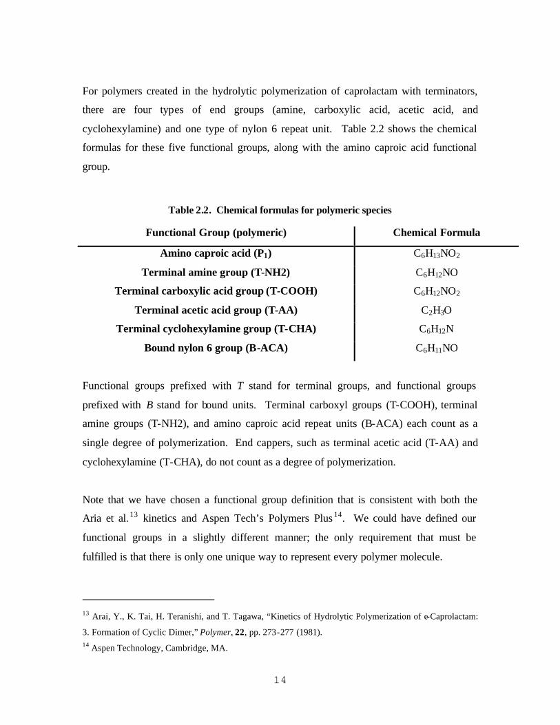
For polymers created in the hydrolytic polymerization of caprolactam with terminators,
there are four types of end groups (amine, carboxylic acid, acetic acid, and
cyclohexylamine) and one type of nylon 6 repeat unit. Table 2.2 shows the chemical
formulas for these five functional groups, along with the amino caproic acid functional
group.
Table 2.2. Chemical formulas for polymeric species
Functional Group (polymeric) Chemical Formula
Amino caproic acid (P1) C6H13NO2
Terminal amine group (T-NH2) C6H12NO
Terminal carboxylic acid group (T-COOH) C6H12NO2
Terminal acetic acid group (T-AA) C2H3O
Terminal cyclohexylamine group (T-CHA) C6H12N
Bound nylon 6 group (B-ACA) C6H11NO
Functional groups prefixed with T stand for terminal groups, and functional groups
prefixed with B stand for bound units. Terminal carboxyl groups (T-COOH), terminal
amine groups (T-NH2), and amino caproic acid repeat units (B-ACA) each count as a
single degree of polymerization. End cappers, such as terminal acetic acid (T-AA) and
cyclohexylamine (T-CHA), do not count as a degree of polymerization.
Note that we have chosen a functional group definition that is consistent with both the
Aria et al. 13 kinetics and Aspen Tech’s Polymers Plus 14. We could have defined our
functional groups in a slightly different manner; the only requirement that must be
fulfilled is that there is only one unique way to represent every polymer molecule.
13 Arai, Y., K. Tai, H. Teranishi, and T. Tagawa, “Kinetics of Hydrolytic Polymerization of e-Caprolactam:
3. Formation of Cyclic Dimer,” Polymer, 22, pp. 273-277 (1981). 14 Aspen Technology, Cambridge, MA.

15
Now, in order to see how we construct all possible polymer molecules using the
functional groups of Table 2.2, we first split all polymers by their degree of
polymerization (DP): the first group has a DP of one, the second group has a DP two,
and the third group has polymers of DP three and higher. We shall discuss each of these
types in Figure 2.3, Figure 2.4, and Figure 2.5.
Figure 2.3 shows the chemical formulas for polymeric species of degree of
polymerization one.
O
OHNH
H
O
OHN
O
CH3
H
O
CH3
O
NNH
H
O
NHHNH
P1
P1,T-AA
P1,T-CHA
P1,T-AA/T-CHA
P1
T-COOH : T-AA
T-CHA : T-NH2
T-CHA : B-ACA : T-AA
Figure 2.3. Polymeric species with a degree of polymerization of one
We denote polymers using Px,y, where x is the degree of polymerization, and y is the
termination condition. Furthermore, colons denote connectivity, i.e., covalent bonding
between segments.
16
An unterminated polymer of DP one is called P1. This molecule is amino caproic acid.
When the amine group is terminated by a monofunctional acid (acetic acid (AA) in this
case), we call that molecule P1,T-AA. It has two functional groups: a terminal acetic acid
group and a terminal carboxylic acid group.
When the carboxylic acid group is terminated by a monofunctional amine
(cyclohexylamine (CHA) in this case), we call that P1,T-CHA. This molecule has a terminal
cyclohexylamine group and a terminal amine group.
When terminated on both sides, we have P1,T-AA/T-CHA, which is made up of three
functional groups: a terminal cyclohexylamine group, a terminal acetic acid group, and a
nylon 6 repeat unit (B-ACA).
Figure 2.4 shows polymeric species of degree of polymerization two.

17
O
NHH
O
OHN
H
O
CH3
O
N
O
OHN
H
H
O
NHH
O
NHN
H
O
N
O
NHN
H O
CH3
H
P2
P2,T-AA
P2,T-CHA
P2,T-AA/T-CHA
T-COOH : T-NH2
T-COOH : B-ACA : T-AA
T-CHA : B-ACA : T-NH2
T-CHA : B-ACA : B-ACA : T-AA
Figure 2.4. Polymeric species of degree of polymerization two
All polymers of DP two or higher have terminal groups of some kind. Unterminated
polymer of DP two has a terminal carboxyl group and a terminal amine group (P2).
Mono-terminated polymer has a single nylon 6 repeat unit (P2,T-AA and P2,T-CHA). Di-
terminated polymer has two nylon 6 repeat units (P2,T-AA/T-CHA).
We form polymeric species of degree of polymerization three and higher in the following
way. For unterminated polymer, we insert a B-ACAn-2 (B-ACAn meaning B-ACA1st:B-
ACA2nd:…B-ACAn-th) in between the terminal groups, n going from three to infinity (Pn).
For mono-terminated polymer, we substitute the long nylon 6 repeat unit with B-ACAn-1
(Pn,T-AA and Pn,T-CHA). For di-terminated polymer, we substitute a B-ACAn group for the
two existing B-ACA units (Pn,T-AA/T-CHA).

18
O
CH3
O
N
O
OHN
H
H
O
NHH
O
NHN
H
Pn
Pn,T-AA
Pn,T-CHA
Pn,T-AA/T-CHA
T-COOH : [B-ACA]n-2 : T-NH2
O
OHN
O
N
O
NHH
H
H
O
CH3
O
NHN
H
n-2
n-1 T-COOH : [B-ACA]n-1 : T-AA
n-1
T-CHA : [B-ACA]n-1 : T-NH2
n
T-CHA : [B-ACA]n : T-AA
Figure 2.5. Polymeric species of length n, where n goes from three to infinity
For convenience, we tabulate the molecular weights of each functional group below
(Table 2.3).
Table 2.3. Functional group molecular weights
Functional Group Molecular Weight (g/mol)
W 18.01528
CL 113.1595
CD 226.318
AA 60.05256
CHA 99.17596
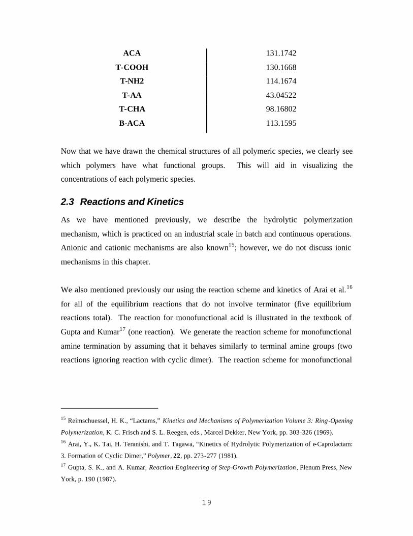
19
ACA 131.1742
T-COOH 130.1668
T-NH2 114.1674
T-AA 43.04522
T-CHA 98.16802
B-ACA 113.1595
Now that we have drawn the chemical structures of all polymeric species, we clearly see
which polymers have what functional groups. This will aid in visualizing the
concentrations of each polymeric species.
2.3 Reactions and Kinetics
As we have mentioned previously, we describe the hydrolytic polymerization
mechanism, which is practiced on an industrial scale in batch and continuous operations.
Anionic and cationic mechanisms are also known15; however, we do not discuss ionic
mechanisms in this chapter.
We also mentioned previously our using the reaction scheme and kinetics of Arai et al.16
for all of the equilibrium reactions that do not involve terminator (five equilibrium
reactions total). The reaction for monofunctional acid is illustrated in the textbook of
Gupta and Kumar17 (one reaction). We generate the reaction scheme for monofunctional
amine termination by assuming that it behaves similarly to terminal amine groups (two
reactions ignoring reaction with cyclic dimer). The reaction scheme for monofunctional
15 Reimschuessel, H. K., “Lactams,” Kinetics and Mechanisms of Polymerization Volume 3: Ring-Opening
Polymerization, K. C. Frisch and S. L. Reegen, eds., Marcel Dekker, New York, pp. 303-326 (1969). 16 Arai, Y., K. Tai, H. Teranishi, and T. Tagawa, “Kinetics of Hydrolytic Polymerization of e-Caprolactam:
3. Formation of Cyclic Dimer,” Polymer, 22, pp. 273-277 (1981). 17 Gupta, S. K., and A. Kumar, Reaction Engineering of Step-Growth Polymerization , Plenum Press, New
York, p. 190 (1987).
20
amine is suggested in Heikens et al. 18 We shall illustrate each of these eight equilibrium
reactions shortly.
The five main equilibrium reactions, by name, are (1) ring opening of caprolactam, (2)
polycondensation, (3) polyaddition of caprolactam, (4) ring opening of cyclic dimer, and
(5) polyaddition of cyclic dimer. Monofunctional acid reacts through the monofunctional
acid condensation mechanism, while monofunctional amine reacts through both
monofunctional amine caprolactam addition and monofunctional amine
polycondensation (all eight of these equilibrium reactions are found in Figure 2.6 through
Figure 2.13).
The rate constant values apply to polymerizations taking place at temperatures ranging
from 230 to 280 °C and initial water concentrations of 0.42 to 1.18 mol/kg. Species
concentrations were experimentally measured using Karl-Fisher water analysis and gas
chromatography19.
This reaction scheme contains two assumptions: the equal reactivity assumption and the
assumption that no cyclics higher than dimer are formed. The equal reactivity
assumption treats the reactivity of polymers as independent of chain length, while having
no cyclic trimer or higher means that we do not track the production or destruction of
these species.
The cyclic dimer assumption is a good approximation, as the majority of the cyclic
oligomers exists as cyclic dimer20, 21. Hermans et al. 22, 23 have confirmed the correctness
18 Heikens, D., P. H. Hermans, and G. M. Van Der Want, “On the Mechanism of the Polymerization of e-
Caprolactam. IV. Polymerization in the Presence of Water and Either an Amine or a Carboxylic Acid,”
Journal of Polymer Science, XLIV, pp. 437-448 (1960). 19 Arai, Y., K. Tai, H. Teranishi, and T. Tagawa, “Kinetics of Hydrolytic Polymerization of e-Caprolactam:
3. Formation of Cyclic Dimer,” Polymer, 22, pp. 273-277 (1981). 20 Arai, Y., K. Tai, H. Teranishi, and T. Tagawa, “Kinetics of Hydrolytic Polymerization of e-Caprolactam:
3. Formation of Cyclic Dimer,” Polymer, 22, pp. 273-277 (1981).
21
of the equal reactivity of end groups assumption for unterminated nylon systems (and the
resulting Flory-Schultz distribution).
We ignore side reactions such as thermo-oxidative degradation reactions 24 that occur in
the presence of oxygen and high heat. These reactions produce carbon monoxide, carbon
dioxide, acetaldehyde, formaldehyde, and methanol. These reactions do not occur
because oxygen is typically excluded from commercial nylon 6 polymerizations 25. We
also ignore transamidation reactions 26, i.e., the attack of an internal, polymeric amide
group by an amine end-group, which results in an exchange of end groups and a
randomization of the molecular weight distribution (leading to the Flory-Schulz
distribution):
x y z x z yP P P P+ ++ +� (2.1)
We ignore this reaction because it does not affect the concentration of polymer,
polymeric end groups, or polymer number-average molecular weight.
21 Reimschuessel, H. K., “Nylon 6. Chemistry and Mechanisms,” Journal of Polymer Science:
Macromolecular Reviews, 12, pp. 65-139 (1977). 22 Hermans, P. H., D. Heikens, and P. F. Van Velden, “A Direct Analytical Test of the Flory-Schultz
Distribution in Nylon 6 Type Equilibrium Polymers. Preliminary Communication,” Journal of Polymer
Science, 16, pp. 451-457 (1955). 23 Hermans, P. H., D. Heikens, and P. F. Van Velden, “On the Mechanism of the Polymerization of e-
Caprolactam. II. The Polymerization in the Presence of Water,” Journal of Polymer Science, 30, pp. 81-104
(1958). 24 Reimschuessel, H. K., “Nylon 6. Chemistry and Mechanisms,” Journal of Polymer Science:
Macromolecular Reviews, 12, p. 109 (1977). 25 Reimschuessel, H. K., “Nylon 6. Chemistry and Mechanisms,” Journal of Polymer Science:
Macromolecular Reviews, 12, pp. 65-139 (1977). 26 Hermans, P. H., D. Heikens, and P. F. Van Velden, “On the Mechanism of the Polymerization of e-
Caprolactam. II. The Polymerization in the Presence of Water,” Journal of Polymer Science, 30, pp. 81-104
(1958).

22
Arai et al.27 use a mass basis for concentration, i.e., concentrations are expressed in moles
per kg of reaction mixture, rather than moles per liter. Changing to a volume basis may
require adjustment of the kinetic parameters due to volume corrections 28.
We now examine each equilibrium reaction in detail, and write the reactions in terms of
our functional groups and derive corresponding rate expressions.
2.3.1 Ring Opening of Caprolactam
The ring opening reaction involves the reversible opening (hydrolysis) of the caprolactam
ring using water to form amino caproic acid. Ring opening proceeds via a nucleophilic
attack of water on caprolactam. The reverse reaction involves a nucleophilic attack of an
amine end-group on its neighboring carboxyl group.
NH
O
+ OH2
k1
k1'=k1/K1
O
OHNH2
Figure 2.6. Ring opening of caprolactam via water
The functional group notation for this reaction is:
1
1 1 1
k1k ' = k K
CL + W P�����⇀↽����� (2.2)
The rate expression is simply the rate of forward reaction minus the rate of reverse
reaction. Reaction rates are the product of the rate constant and the product of all
27 Arai, Y., K. Tai, H. Teranishi, and T. Tagawa, “Kinetics of Hydrolytic Polymerization of e-Caprolactam:
3. Formation of Cyclic Dimer,” Polymer, 22, pp. 273-277 (1981). 28 Heikens, D., and P. H. Hermans, “On the Mechanism of Polymerization of e-Caprolactam in the
Presence of Water. III. Supplementary Remarks on a Previous Paper. Introduction to Volume Correction,”
Journal of Polymer Science, XLIV, pp. 429-436 (1960).
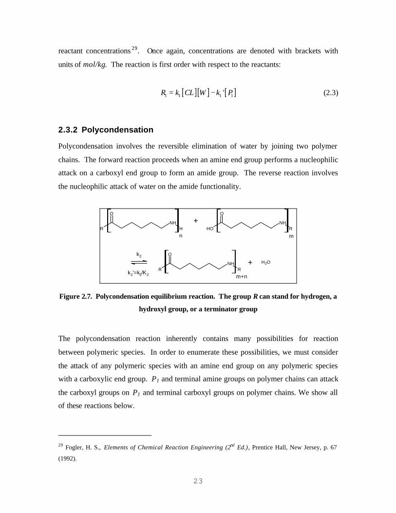
23
reactant concentrations 29. Once again, concentrations are denoted with brackets with
units of mol/kg. The reaction is first order with respect to the reactants:
[ ][ ] [ ]1 1 1 1'R k CL W k P= − (2.3)
2.3.2 Polycondensation
Polycondensation involves the reversible elimination of water by joining two polymer
chains. The forward reaction proceeds when an amine end group performs a nucleophilic
attack on a carboxyl end group to form an amide group. The reverse reaction involves
the nucleophilic attack of water on the amide functionality.
O
RNH
H+
n m
k2
k2'=k2/K2 m+n
+ OH2
O
OHNH
R
O
RNH
R
Figure 2.7. Polycondensation equilibrium reaction. The group R can stand for hydrogen, a
hydroxyl group, or a terminator group
The polycondensation reaction inherently contains many possibilities for reaction
between polymeric species. In order to enumerate these possibilities, we must consider
the attack of any polymeric species with an amine end group on any polymeric species
with a carboxylic end group. P1 and terminal amine groups on polymer chains can attack
the carboxyl groups on P1 and terminal carboxyl groups on polymer chains. We show all
of these reactions below.
29 Fogler, H. S., Elements of Chemical Reaction Engineering (2nd Ed.) , Prentice Hall, New Jersey, p. 67
(1992).

24
2
2 2 2
k1 1 k '=k K
P + P T-COOH:T-NH2 + W������⇀↽������ (2.4)
2
2 2 2
k1 k '=k K
P + T-COOH T-COOH:B-ACA + W ������⇀↽������ (2.5)
2
2 2 2
k1 k '=k K
T-NH2 + P T-NH2:B-ACA + W ������⇀↽������ (2.6)
2
2 2 2
k
k '=k KT-NH2 + T-COOH B-ACA:B-ACA + W ������⇀↽������ (2.7)
The rate expression for reaction (2.4) is the following:
[ ] [ ][ ]2
2 2 1 2 2'R k P k P W= − (2.8)
Note that we have not used a reverse rate term of [ ][ ]2 ' 2k W T NH− ,
[ ][ ]2 'k W T COOH− , or some other variant using functional groups. This is because each
of these terminal group concentrations represents the concentration of all polymer
molecules with these terminal groups. We wish only to consider the reaction of
unterminated P2 molecules.
The rate expression for reaction (2.5) is:
[ ][ ] [ ] [ ] [ ]( )( )3 2 1 2 1, 2' T AAR k P T COOH k W T COOH P P− = − − − − + (2.9)
Note the reverse reaction term above. The reverse reaction concerns terminal carboxyl
groups immediately attached to a B-ACA group. All polymeric species containing T-
COOH groups have B-ACA’s immediately attached except for P2 and P1,T-AA, which have
a terminal amine group or terminal acetic acid group attached to the terminal carboxyl
group, respectively (see Figure 2.3 and Figure 2.4). Therefore, we must subtract the
concentration of these species.
The rate expression for reaction (2.6) is:

25
[ ][ ] [ ] [ ] [ ]( )( )4 2 1 2 1, 22 ' 2 T CHAR k T NH P k W T NH P P− = − − − − + (2.10)
Lastly, for reaction (2.7), the rate expression is:
[ ][ ] [ ][ ]5 2 22 ' :R k T NH T COOH k W B ACA B ACA= − − − − − (2.11)
Determining the concentration of B-ACA linkages is the trickiest step of this analysis.
Let us start by considering the concentration of B-ACA units:
[ ] [ ]:B ACA B ACA B ACA− − = − … (2.12)
We must subtract from this the concentration of doubly terminated monomer, singly
terminated dimer, and unterminated trimer (see Figure 2.3, Figure 2.4, and Figure 2.5):
[ ] [ ]
[ ]( )1, / 2, 2, 3
:
T A A T CHA T AA T CHA
B ACA B ACA B ACA
P P P P− − − −
− − = −
− + + + … (2.13)
Now what we are left with is the concentration of B-ACA groups in only those polymers
that have at least two of these groups. We must eliminate one B-ACA from this number
for every polymer chain, e.g., a five-B-ACA chain has four B-ACA:B-ACA linkages.
We do so by subtracting a single type of end group: we can either choose T-NH2 and T-
AA, or T-COOH and T-CHA:
[ ] [ ][ ]( )
[ ] [ ] [ ]( )[ ] ( )[ ] [ ] [ ] [ ]
1, / 2, 2, 3
1, 2 2, 3
1, 1, / 2,
1, 2 1,
:
2
2
T AA T CHA T AA T CHA
T CHA T CHA
T AA T AA T CHA T AA
T CHA T AA
B ACA B ACA B ACA
P P P P
T NH P P P P
T AA P P P
B ACA T NH T AA P P P
− − − −
− −
− − − −
− −
− − = −
− + + +
− − + + + +
− − + + +
= − − − − − + + +
(2.14)

26
We want to subtract end groups for only those polymers with two or more B-ACA repeat
units; hence the origin of the additional terms such as [ ] [ ]( )1, 2 2, 3T CHA T CHAP P P P− − + + +
and ( )1, 1, / 2,T AA T A A T CHA T AAP P P− − − − + + associated with smaller polymeric species
containing the respective end group.
2.3.3 Polyaddition of Caprolactam
Polyaddition proceeds when the amine group of a nylon molecule opens a caprolactam
ring:
+ NH
O
n+1
k3
k3'=k3/K3
O
RNH
H
n
O
RNH
H
Figure 2.8. Addition of caprolactam
Any polymer with an amine functionality can perform the forward reaction. We list all of
the possibilities below:
3
3 3 3
k1 k '=k K
P + CL T-NH2:T-COOH�����⇀�↽������ (2.15)
3
3 3 3
k
k '=k KT-NH2 + CL T-NH2:B-ACA�����⇀�↽������ (2.16)
The rate expression for reaction (2.15) is:
[ ][ ] [ ]6 3 1 3 2'R k P CL k P= − (2.17)
The rate expression for reaction (2.16) is:
[ ][ ] [ ] [ ]( )( )7 3 3 1, 22 ' 2 T CHAR k T NH CL k T NH P P− = − − − − + (2.18)

27
The last concentration term represents the terminal amine groups attached to a B-ACA
repeat unit.
2.3.4 Ring Opening of Cyclic Dimer
Cyclic dimer can be opened by water; this reaction is analogous to ring opening of
caprolactam.
NH
NH
O
O
+ OH2
2
k4
k4'=k4/K4
O
OHNH
H
Figure 2.9. Ring-opening of cyclic dimer
In our notation system, we represent this reaction as:
4
4 4 4
k
k '=k KCD + W T-COOH:T-NH2������⇀↽������ (2.19)
The rate expression for this reaction is:
[ ][ ] [ ]8 4 4 2'R k CD W k P= − (2.20)
2.3.5 Polyaddition of Cyclic Dimer
We also consider polyaddition of cyclic dimer; this reaction is analogous to the
polyaddition of caprolactam.

28
+k5
k5'=k5/K5
O
RNH
H
n
O
RNH
H
NH
NH
O
O
n+2
Figure 2.10. Polyaddition of cyclic dimer
A terminal amine group of any polymer can perform this addition. Therefore, over all
polymer species, we have:
5
5 5 5
k1 k '=k K
P + CD T-NH2:B-ACA:T-COOH�����⇀�↽������ (2.21)
5
5 5 5
k
k '=k KT-NH2 + CD B-ACA:B-ACA:T-NH2�����⇀�↽������ (2.22)
The rate expression for reaction (2.21) is:
[ ][ ] [ ]9 5 1 5 3'R k P CD k P= − (2.23)
The rate expression for reaction (2.22) is:
[ ][ ] [ ] [ ] [ ]( )( )10 5 5 1, 2 2, 32 ' 2 T CHA T CHAR k T NH CD k T NH P P P P− − = − − − − + + + (2.24)
The last concentration term represents the concentration of only those terminal amine
groups that are attached to two B-ACA units.
2.3.6 Monofunctional Acid Condensation
Monofunctional acids react with terminal amine groups to form “acid end capped”
polymer species and water.

29
+
n
k2
k2'=k2/K2
O
RNH
H
n
O
RNH
O
CH3
O
OH
CH3
OH2+
Figure 2.11. Monofunctional acid termination
We assume that the rate constant is identical to that of condensation reactions since the
mechanism is the same.
All polymers with a terminal amine can undergo acid end capping:
2
2 2 2
k1 k '=k K
P + AA T-AA:T-COOH + W������⇀↽������ (2.25)
2
2 2 2
k
k '=k KT-NH2 + AA B-ACA:T-AA + W������⇀↽������ (2.26)
The rate expressions for these reactions are below:
[ ][ ] [ ]11 2 1 2 1,' T AAR k AA P k P W− = − (2.27)
[ ][ ] [ ] [ ]( )12 2 2 1,2 ' T AAR k AA T NH k W T AA P − = − − − − (2.28)
2.3.7 Monofunctional Amine Caprolactam Addition
Monofunctional amines can add caprolactam just as polymeric terminal amines do:
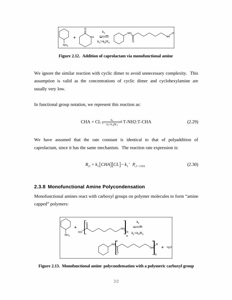
30
+ NH
Ok3
k3'=k3/K3NH2
O
NHHNH
Figure 2.12. Addition of caprolactam via monofunctional amine
We ignore the similar reaction with cyclic dimer to avoid unnecessary complexity. This
assumption is valid as the concentrations of cyclic dimer and cyclohexylamine are
usually very low.
In functional group notation, we represent this reaction as:
3
3 3 3
k
k '=k KCHA + CL T-NH2:T-CHA�����⇀�↽������ (2.29)
We have assumed that the rate constant is identical to that of polyaddition of
caprolactam, since it has the same mechanism. The reaction rate expression is:
[ ][ ]13 3 3 1,' T CHAR k CHA CL k P − = − (2.30)
2.3.8 Monofunctional Amine Polycondensation
Monofunctional amines react with carboxyl groups on polymer molecules to form “amine
capped” polymers:
+NH2
O
NHRNH
O
OHNH
R
k2
k2'=k2/K2
+ OH2
n
n
Figure 2.13. Monofunctional amine polycondensation with a polymeric carboxyl group

31
Polymeric carboxyl groups are found on some linear monomers and unterminated higher
polymers:
2
2 2 2
k1 k '=k K
CHA + P T-NH2:T-CHA + W������⇀↽������ (2.31)
2
2 2 2
k
k '=k KCHA + T-COOH B-ACA:T-CHA + W������⇀↽������ (2.32)
The rate expressions for these reactions are below:
[ ][ ] [ ]14 2 1 2 1,' T CHAR k CHA P k P W− = − (2.33)
[ ][ ] [ ] [ ]( )15 2 2 1,' T CHAR k CHA T COOH k W T CHA P − = − − − − (2.34)
2.3.9 Concentration of Terminated and Unterminated Linear
Monomers and Dimers
Now that we have defined all reaction rate expressions, we must consider their solution.
One weakness of not explicitly keeping track of each polymeric species is that we do not
have specific information about the connectivity of functional groups. For example, we
would not be able to answer the following question: how many polymers are created
with a degree of polymerization of ten and are acetic acid terminated? We only know
with absolute certainty how many amino caproic acid molecule s, i.e., P1, exist, because
we track this group explicitly. This result begs the following question about our analysis
so far: how are we to determine the concentration of species such as P2, P1,T -AA, P2,T-CHA,
etc.?

32
The first assumption that is typically made30 is that unterminated species of DP one
through three have equal concentrations:
[ ] [ ] [ ]1 2 3P P P= = (2.35)
Arai and coworkers31 found that the results of kinetics simulations did not vary as the
concentrations of linear dimer and trimer were changed within the neighborhood of that
of amino caproic acid. Furthermore, experimental results32 approximately validate this
assumption.
We now extend this result to terminated species up to DP two:
1, 2,y yP P = (2.36)
Now, for a distribution of polymers according to length and acetic-acid termination
condition, there is a fraction that is one repeat unit long:
[ ] ( )( )1, 1,T AAP T AA P DP T AA− = − = − (2.37)
( )1,P DP T AA= − is the probability that we will find a polymer of DP one among all
acetic acid terminated polymers. We now assume that the probability of finding a
polymer of DP one among all acetic acid terminated polymers is equal to the probability
of finding a polymer of DP one among all polymers P(DP=1).
30 Arai, Y., K. Tai, H. Teranishi, and T. Tagawa, “Kinetics of Hydrolytic Polymerization of e-Caprolactam:
3. Formation of Cyclic Dime r,” Polymer, 22, pp. 273-277 (1981). 31 Arai, Y., K. Tai, H. Teranishi, and T. Tagawa, “Kinetics of Hydrolytic Polymerization of e-Caprolactam:
3. Formation of Cyclic Dimer,” Polymer, 22, pp. 273-277 (1981). 32 Mochizuki, S., and N. Ito, “The Hydrolytic Poly merization Kinetics of e-Caprolactam,” Chemical
Engineering Science, 28, pp. 1139-1147 (1973).

33
Now the following question naturally arises: how do we compute the probability of
finding a polymer of any length? We assume that our polymer molecular weight follows
the Flory-Schultz most-probable distribution – a theoretical result33 obtained from the
analysis of the condensation polymerization of bi-functional monomer (such as amino
caproic acid). Two important expressions regarding the most-probable distribution come
from Flory’s textbook34: an expression for the mole-fraction of a polymer species of DP
x, and an expression for the number-average DP nx as a function of conversion p.
( ) 11 xxNp p
N−= − (2.38)
1
1nxp
=−
(2.39)
When we combine these two equations, and set x equal to one, we get the following mole
fraction (or probability) of polymers of length one:
( )1 1
1
n
NP DP
N
x
= =
= (2.40)
We use this expression, along with equations (2.36) and (2.37), to generate the
concentration terms that we need to evaluate reaction rates:
[ ]1,
1T AA
n
P T AAx− = − (2.41)
[ ]1, 2,
1T CHA T CHA
n
P P T CHAx− − = = − (2.42)
33 Flory, P. J., Principles of Polymer Chemistry, Cornell University Press, New York, pp. 69-105 (1953). 34 Flory, P. J., Principles of Polymer Chemistry, Cornell University Press, New York, p. 81, 320 (1953).

34
2.3.10 Reaction and Rate Summary
We summarize Sec. 2.3 by tabulating all of our equilibrium reactions and accompanying
rates (Table 2.4).
Table 2.4. Summary of equilibrium reactions and accompanying reaction rates
Equilibrium Reaction Reaction Rate
1
1 1 1
k
k ' = k K
1
CL + W
P
�����⇀↽�����
[ ][ ][ ]
1 1
1 1'
R k CL W
k P
=
−
2
2 2 2
k1 1 k '=k K
P + P
T-COOH:T-NH2 + W
������⇀↽������ [ ][ ][ ]
22 2 1
2 1'
R k P
k P W
=
−
2
2 2 2
k1 k '=k K
P + T-COOH
T-COOH:B-ACA + W
������⇀↽������
[ ][ ]
[ ][ ]
[ ] [ ]
3 2 1
21
' 1
n
R k P T COOH
T COOHk W
P T AAx
= −
−
− − − −
2
2 2 2
k1 k '=k K
T-NH2 + P
T-NH2:B-ACA + W
������⇀↽������
[ ][ ]
[ ][ ]
[ ] [ ]
4 2 1
21
2
2' 1
n
R k T NH P
T NHk W
P T CHAx
= −
−
− − − −
2
2 2 2
k
k '=k KT-NH2 + T-COOH
B-ACA:B-ACA + W
������⇀↽������
[ ][ ]
[ ][ ] [ ] [ ]
[ ] [ ] [ ]
5 2
21
2
2' 1 1
n n
R k T NH T COOH
B ACA T NH T AAk W
P T AA T CHAx x
= − −
− − − − −
− + + − + −
3
3 3 3
k1 k '=k K
P + CL
T-NH2:T-COOH
�����⇀�↽������ [ ][ ][ ]
6 3 1
3 1'
R k P CL
k P
=
−

35
3
3 3 3
k
k '=k KT-NH2 + CL
T-NH2:B-ACA
�����⇀�↽������
[ ][ ][ ]
[ ] [ ]
7 3
31
2
2' 1
n
R k T NH CL
T NHk
P T CHAx
= −
−
− − − −
4
4 4 4
k
k '=k KCD + W
T-COOH:T-NH2
������⇀↽������ [ ][ ][ ]
8 4
4 1'
R k CD W
k P
=
−
5
5 5 5
k1 k ' = k K
P + CD
T-NH2:B-ACA:T-COOH
�����⇀�↽������ [ ][ ][ ]
9 5 1
5 1'
R k P CD
k P
=
−
5
5 5 5
k
k ' = k KT-NH2 + CD
B-ACA:B-ACA:T-NH2
�����⇀�↽������
[ ][ ][ ]
[ ] [ ]
10 5
51
2
2' 1
2 2n
R k T NH CD
T NHk
P T CHAx
= −
−
− − − −
2
2 2 2
k1 k '=k K
P + AA
T-AA:T-COOH + W
������⇀↽������ [ ][ ]
[ ][ ]11 2 1
21
'n
R k AA P
k W T AAx
=
− −
2
2 2 2
k
k '=k KT-NH2 + AA
B-ACA:T-AA + W
������⇀↽������ [ ][ ]
[ ][ ]
12 2
2
2
1' 1
n
R k AA T NH
k W T AAx
= −
− − −
3
3 3 3
k
k ' = k KCHA + CL
T-NH2:T-CHA
�����⇀�↽������ [ ][ ]
[ ]13 3
31
'n
R k CHA CL
k T CHAx
=
− −
2
2 2 2
k1 k '=k K
CHA + P
T-NH2:T-CHA + W
������⇀↽������ [ ][ ]
[ ][ ]14 2 1
21
'n
R k CHA P
k W T CHAx
=
− −
2
2 2 2
k
k '=k KCHA + T-COOH
B-ACA:T-CHA + W
������⇀↽������ [ ][ ]
[ ][ ]
15 2
21
' 1n
R k CHA T COOH
k W T CHAx
= −
− − −

36
The rate constants are found in Arai et al.35 (Table 2.5). We have converted the numbers
into SI units. All reactions are catalyzed by carboxylic acid functional groups36, 37. We
have ignored the presence of alkali metal compounds that also have a catalytic effect38.
35 Arai, Y., K. Tai, H. Teranishi, and T. Tagawa, “Kinetics of Hydrolytic Polymerization of e-Caprolactam:
3. Formation of Cyclic Dimer,” Polymer, 22, pp. 273-277 (1981). 36 Giori, C., and B. T. Hayes, “Hydrolytic Polymerization of Caprolactam. I. Hydrolysis –
Polycondensation Kinetics,” Journal of Polymer Science, Part A-1, 8, pp. 335-349 (1970). 37 Heikens, D., P. H. Hermans, and G. M. Van Der Want, “On the Mechanism of the Polymerization of e-
Caprolactam. IV. Polymerization in the Presence of Water and Either an Amine or a Carboxylic Acid,”
Journal of Polymer Science, XLIV, pp. 437-448 (1960). 38 Khaitin, B. S., “Mathematical Modelling of Caprolactam Polymerization,” Polymer Science USSR, 24(5),
pp. 1091-1096 (1982).
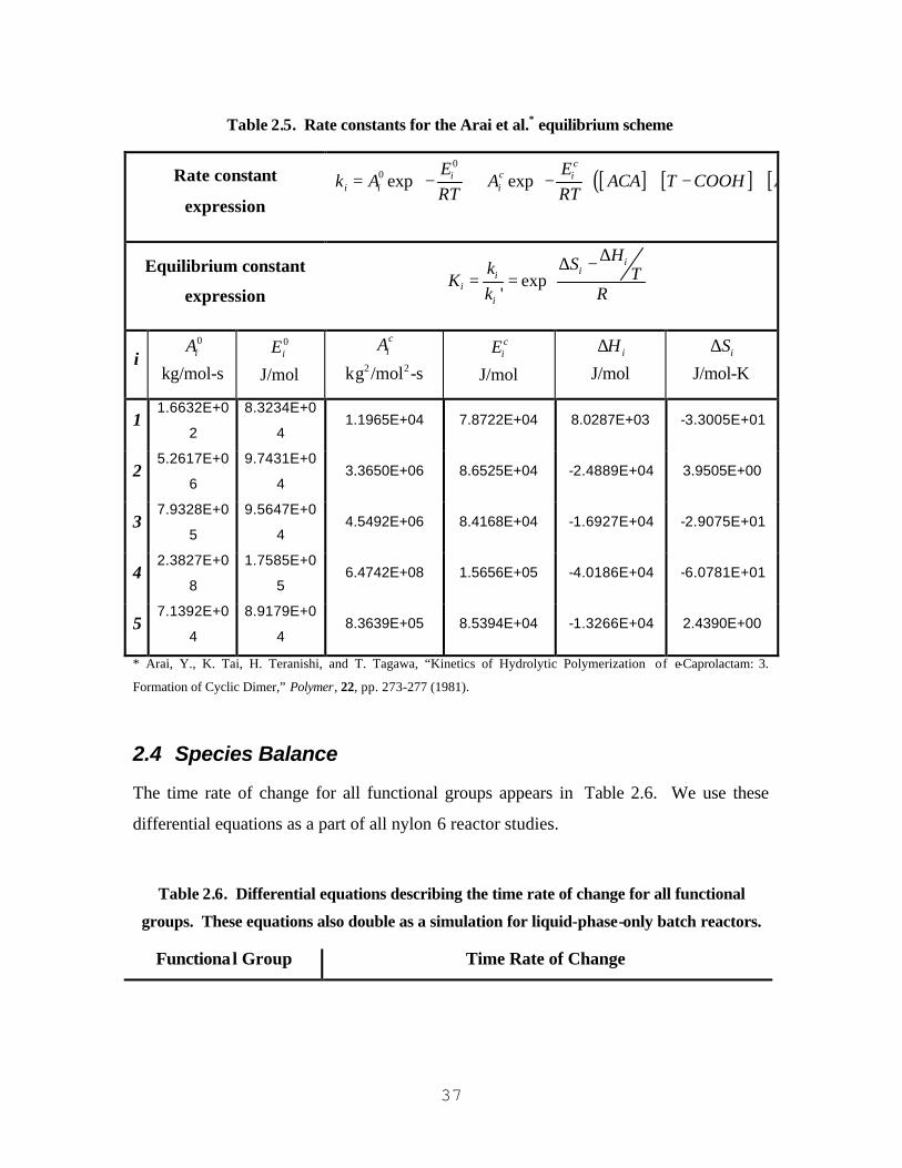
37
Table 2.5. Rate constants for the Arai et al.* equilibrium scheme
Rate constant
expression [ ] [ ] [(
00 exp exp
cci i
i i i
E Ek A A ACA T COOH AA
RT RT
= − + − + − +
Equilibrium constant
expression exp
'
iii
ii
HSk TKk R
∆ ∆ − = =
i 0
kg/mol-siA
0
J/moliE
2 2kg /mol -s
ciA
J/mol
ciE
J/moliH∆
J/mol-K
iS∆
1 1.6632E+0
2
8.3234E+0
4 1.1965E+04 7.8722E+04 8.0287E+03 -3.3005E+01
2 5.2617E+0
6
9.7431E+0
4 3.3650E+06 8.6525E+04 -2.4889E+04 3.9505E+00
3 7.9328E+0
5
9.5647E+0
4 4.5492E+06 8.4168E+04 -1.6927E+04 -2.9075E+01
4 2.3827E+0
8
1.7585E+0
5 6.4742E+08 1.5656E+05 -4.0186E+04 -6.0781E+01
5 7.1392E+0
4
8.9179E+0
4 8.3639E+05 8.5394E+04 -1.3266E+04 2.4390E+00
* Arai, Y., K. Tai, H. Teranishi, and T. Tagawa, “Kinetics of Hydrolytic Polymerization of e-Caprolactam: 3.
Formation of Cyclic Dimer,” Polymer, 22, pp. 273-277 (1981).
2.4 Species Balance
The time rate of change for all functional groups appears in Table 2.6. We use these
differential equations as a part of all nylon 6 reactor studies.
Table 2.6. Differential equations describing the time rate of change for all functional
groups. These equations also double as a simulation for liquid-phase-only batch reactors.
Functional Group Time Rate of Change

38
W [ ]
( )2 3 4 5 11 12 14 15
1 8
d WR R R R R R R R
dtR R
= + + + + + + +
− +
CL [ ] ( )1 6 7 13
d CLR R R R
dt= − + + +
CD [ ] ( )8 9 10
d CDR R R
dt= − + +
AA [ ] ( )11 12
d AAR R
dt= − +
CHA [ ] ( )13 14 15
d CHAR R R
dt= − + +
P1
[ ]
( )
11
2 3 4 6 9 11 142
d PR
dtR R R R R R R
=
− + + + + + +
B-ACA [ ]3 4 5 7 9 10 12 152 2
d B ACAR R R R R R R R
dt
−= + + + + + + +
T-NH2 [ ]
( )2 6 8 9 13 14
5 12
2d T NHR R R R R R
dtR R
−= + + + + +
− +
T-COOH [ ]
( )2 6 8 9 11
5 15
d T COOHR R R R R
dtR R
−= + + + +
− +
T-AA [ ]11 12
d T AAR R
dt
−= +
T-CHA [ ]13 14 15
d T CHAR R R
dt
−= + +
The initial condition for each of these equations is the initial concentration.
2.5 Polymer Properties
The equations in Table 2.6 allow us to simulate concentration changes in all functional
groups. Now we must solve for polymer properties: polymer mass, number-average

39
molecular weight, end-group concentrations, formic-acid viscosity, and the content of
extractables.
The polymer mass is simply the mass-concentration (kg/kg total) of all of the polymeric
functional groups and amino caproic acid, multiplied by the total mass of the system:
( )
( )( )
( )( )
( )2
Polymer Mass, kg =
kgmol, , kg mol
kgmol, , kg mol
kgmol, , kg molTotal mass, kg
kgmol2, , kg mol
kgmol, , kg mol
,
ACA
B ACA
T COOH
T NH
T AA
ACA MW
B ACA MW
T COOH MW
T NH MW
T AA MW
T CHA
−
−
−
−
+ − + − + − + −
+ − ( )kgmol , kg molT CHAMW −
(2.43)
We compute the polymer number-average degree of polymerization nx using the
following formula39:
[ ]
[ ]n
nn
n Px
P= ∑
∑ (2.44)
The numerator represents the total number of functional groups that count as repeat units
over all polymeric species, or [ ] [ ] [ ] [ ]2B ACA T COOH T NH ACA− + − + − + . The
denominator represents the number of polymer chains. Each polymer chain is either an
amino caproic acid or has a terminal amine group or is terminated with an acetic acid
39 Cowie, J. M. G., Polymers: Chemistry and Physics of Modern Materials (2nd Ed.) , Blackie Academic and
Professional, New York, p. 8 (1991).

40
group. Therefore, the number of chains is the sum of the number of amine end-groups,
amino caproic acid groups, and terminal acetic acid groups:
[ ] [ ] [ ] [ ]
[ ] [ ] [ ]2
2n
B ACA T COOH T NH ACAx
ACA T NH T AA− + − + − +
=+ − + −
(2.45)
The corresponding number-average molecular weight is determined by considering the
molecular weight of each functional group, this time including terminal acetic acid and
cyclohexylamine groups:
[ ] [ ] [ ][ ] [ ] [ ]
[ ] [ ] [ ]
22
2
B ACA T COOH T NH
T AA T CHA ACAn
B ACA MW T COOH MW T NH MW
T AA MW T CHA MW ACA MWM
ACA T NH T AA
− − −
− −
− + − + − + − + − + =
+ − + − (2.46)
The end-group concentrations are typically expressed in mmol/kg (or eq/106 g):
mmolAmine group concentration, kg
1,000 mmol mol mol 2, , mol kg kgT NH ACA
=
− +
(2.47)
mmolCarboxylic acid group concentration, kg
1,000 mmol mol mol , , mol kg kgT COOH ACA
=
− +
(2.48)
Amine groups, R-NH2, occur as terminal amine groups and amino caproic acid
molecules. Carboxylic acid groups, R-COOH, occur as terminal carboxylic acid groups
and amino caproic acid molecules.
To calculate end-group concentrations in pure polymer, we multiply the results of
equations (2.47) and (2.48) by the total mass of the liquid phase (kg) and then divide by
the total mass of the polymer (kg).

41
We also give an equation to estimate the formic acid viscosity (FAV) using the polymer
molecular weight. The FAV is experimentally determined by first dissolving 22 grams of
polyamide in 8 oz. of formic acid 40. The viscosity of the solution is then determined,
along with the viscosity of formic acid alone. The ratio of the solution to solvent
viscosity is the FAV. We approximate the FAV using the polymer molecular weight41:
( )2.159.38 9 2 nFAV E M= − (2.49)
We have assumed that the final polydispersity of the polymer is two, a theoretical result
of the Flory-Schultz distribution. This has been found to be the case in theoretical studies
of acetic-acid-terminated nylon 642. A FAV data point found in US Patent #3,294,75643
tells us that a number-average molecular weight of 18,000 g/mol corresponds with an
FAV of 55. This data point is well correlated with equation (2.49).
We approximate the mass-percentage of extractables using the mass-percentage of all
non-polymeric species:
40 ASTM D789 41 Akkapeddi, M. K., C. Brown, and B. Vanbuskirk, “Chain Extension of PA-6 and PA-6/66 Copolymer
Via Reactive Extrusion with Triscaprolactamyl Phosphite (TCP),” Honeywell Report,
http://www.honeywell-plastics.com/techinfo/techpapers/0475.pdf, p. 3. 42 Agrawal, A. K., K. Devika, and T. Manabe, “Simulation of Hydrolytic Polymerization of Nylon-6 in
Industrial Reactors: Part I. Mono-Acid-Stabilized Systems in VK Tube Reactors,” Industrial and
Engineering Chemistry and Research, 40, pp. 2563-2572 (2001). 43 Russell, W. N., A. H. Wiesner, and O. E. Snider, “Continuous Polymerization of E-Caprolactam,” US
Patent #3,294,756 , pp. 1-7 (1966).
42
[ ] [ ] [ ][ ] [ ][ ] [ ] [ ][ ] [ ] [ ]
2
g/kg Small Molecules =
g/kg Polymer = 2
g/kg Small Molecules% Extractables
g/kg Small Molecul
W AA CL
CD CHA
ACA B ACA T NH
T COOH T AA T CHA
W MW AA MW CL MW
CD MW CHA MW
ACA MW B ACA MW T NH MW
T COOH MW T AA MW T CHA MW− −
− − −
+ +
+ +
+ − + −
+ − + − + −
∼es + g/kg Polymer
(2.50)
2.6 Batch Reactor Simulation
We use the differential equations of Table 2.6 to simulate a batch, nylon 6
polymerization. We do not need additional reactor equations to simulate a batch reactor;
therefore, it makes for a suitable example to study the kinetics of nylon 6
polymerizations.
The core of the batch reactor simulation is solving the ordinary differential equations in
Table 2.6. All other quantities, such as polymer properties and mass of each component,
are post calculated. We give a simulation example written in FORTRAN 77 in the
appendix for this chapter. We call the IMSL subroutine IVPAG to solve the ordinary
differential equation system.
We simulate a system that is initially charged with 99 kg of caprolactam and 1 kg of
water. The batch reactor operates at 240 °C for ten hours, after which the molten
polymer is discharged. The reactor is operated at high pressure, i.e., we simulate it as a
single liquid phase.
The first notable point regarding the polymerization is the relationship between total ends
and conversion rate (Figure 2.14). The significance of this plot was first pointed out in
Yates et al.44 44 Yates, S. L., C. J. Cole, A. H. Wiesner, and J. W. Wagner, “Two-Stage Hydrolysis Process for the
Preparation of Nylon 6,” United States Patent 4,310,659, Allied Corporation, pp. 1-7 (1982).
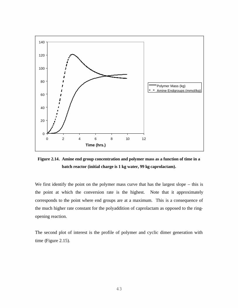
43
0
20
40
60
80
100
120
140
0 2 4 6 8 10 12
Time (hrs.)
Polymer Mass (kg)Amine Endgroups (mmol/kg)
Figure 2.14. Amine end group concentration and polymer mass as a function of time in a
batch reactor (initial charge is 1 kg water, 99 kg caprolactam).
We first identify the point on the polymer mass curve that has the largest slope – this is
the point at which the conversion rate is the highest. Note that it approximately
corresponds to the point where end groups are at a maximum. This is a consequence of
the much higher rate constant for the polyaddition of caprolactam as opposed to the ring-
opening reaction.
The second plot of interest is the profile of polymer and cyclic dimer generation with
time (Figure 2.15).

44
0
0.05
0.1
0.15
0.2
0.25
0.3
0.35
0.4
0.1 1.1 2.1 3.1 4.1 5.1 6.1 7.1 8.1 9.1
Time (hrs.)
Cyc
lic D
imer
Mas
s (k
g)
0
10
20
30
40
50
60
70
80
90
100
Po
lym
er M
ass
(kg
)
Cyclic DimerPolymer Mass
Figure 2.15. Cyclic dimer and polymer production vs. time in a liquid-only batch reactor
(initial charge is 1 kg water, 99 kg caprolactam).
Cyclic dimer production continues throughout the course of polymerization. In fact, as
the polymer mass reaches equilibrium in the reaction mixture, cyclic dimer continues to
be produced at a high rate.
If we add 0.21 kg (reference 45 instructs us to add terminator in the ratio of 0.2 to 0.4
moles of terminator per 100 moles of caprolactam) of acetic acid to the reaction mass, we
increase the rate of polymerization significantly because of the presence of a higher
amount of carboxylic acid groups (Figure 2.16):
45 Twilley, I. C., D. W. H. Roth, and R. A. Lofquist, “Process for the Production of Nylon 6,” US Patent
#3,558,567, Allied Chemical Corporation

45
0
20
40
60
80
100
120
140
0 2 4 6 8 10 12
Time (hrs.)
Polymer Mass (kg)Amine Endgroups (mmol/kg)Polymer Mass (AA-term.)Amine Endgroups (AA-term.)
Figure 2.16. Addition of acetic acid increases the rate of polymerization via increase in
carboxylic acid functionalities (initial charge is 1 kg water, 99 kg caprolactam, and 0.21 kg
acetic acid).
The maximum amine end-group concentration is somewhat depressed over the base case
– we expect this result since acetic acid caps terminal amine groups.
When we further add 0.35 kg of cyclohexylamine terminator, we do not change the
conversion characteristics of the reaction (Figure 2.17).

46
0
20
40
60
80
100
120
140
0 2 4 6 8 10 12
Time (hrs.)
Polymer Mass (kg, AA-term.)
Amine Endgroups (mmol/kg,AA-term.)Polymer Mass (AA/CHA-term.)Amine Endgroups (AA/CHA-term.)
Figure 2.17. Acetic acid/cyclohexylamine terminated nylon 6 batch polymerization (initial
charge is 1 kg water, 99 kg caprolactam, 0.21 kg acetic acid, and 0.35 kg cyclohexylamine).
Cyclohexylamine does not catalyze the step-growth reactions; therefore, we should not
expect it to affect the rate of polymerization. However, the addition of cyclohexylamine
tends to somewhat increase the overall amine end-group concentration.
2.7 Conclusions
We have developed a functional group model for the polymerization of e-caprolactam.
To our knowledge, this model has not appeared in the literature. The advantages of the
functional group model over the previously used method-of-moments approach are:
• The functional group approach is more intuitive to develop and apply – e.g., no
additional knowledge above basic reaction kinetics (such as statistics) is required

47
• The functional group approach easily handles modifications to the
terminator/reactions set – i.e., additional reactions are simply appended to the
existing kinetic scheme without a need for re-deriving moment expressions
After we show the development of the kinetics set, we apply it a simulation of a nylon 6
batch reactor. We briefly show some characteristics of the polymerization, and then
show how to optimize the process using a design-of-experiments approach. High
reaction temperatures, water, and acetic acid initial charges are key to reducing batch
times and cyclic dimer production; however, molecular weight build tends to suffer.

48
2.8 Nomenclature
Symbol Description Units
Ai0 Pre-exponential factor for uncatalyzed
forward reaction i kg/mol-s
Aic Pre-exponential factor for catalyzed
forward reaction i kg/mol-s
Ei0 Activation energy for uncatalyzed
forward reaction i J/mol
Eic Activation energy for catalyzed
forward reaction i J/mol
FAV Formic-acid viscosity Unitless
iH∆ enthalpy of reaction i J/mol
Ki Equilibrium constant for reaction i Unitless
ki Forward rate constant for reaction i kg/mol-s
ki’ Reverse rate constant for reaction i kg/mol-s
nM Number-average molecular weight kg/mol
p Conversion Unitless
Px Polymer chain with degree of polymerization x N. A.
Px,y Polymer chain with degree of polymerization x and
termination condition y N. A.
Ri Rate equation for reaction i N. A.
iS∆ Entropy of reaction i J/mol-K
nx Number-average degree of polymerization Unitless

49
2.9 Appendix – FORTRAN 77 Code for Nylon-6 Batch Reactor
Simulation (DIGITAL Visual FORTRAN 6.0)
USE NUMERICAL_LIBRARIES INTEGER N, NPARAM PARAMETER (N=11, NPARAM=50) C SPECIFICATIONS FOR LOCAL VARIABLES INTEGER IDO, IEND, NOUT, I REAL A(1,1), PARAM(NPARAM), T, TEND, TOL, Y(N), TIMEEND REAL MOLWEIGHT(N), MASS(N), TOTALMASS, POLYMERMASS REAL TIMEINTERVAL, MN, FAV, AMINE, CARBOX, EXTRACT C SPECIFICATIONS FOR FUNCTIONS EXTERNAL FCN, FCNJ COMMON XN C OPEN OUTPUT FILE AND INITIALIZE SOLVER PARAMETERS OPEN(9,FILE='NYLONBATCH.DAT') C CALL SSET (NPARAM, 0.0, PARAM, 1) C IDO = 1 C MOLECULAR WEIGHTS MOLWEIGHT(1) = 18.01528 MOLWEIGHT(2) = 113.1595 MOLWEIGHT(3) = 226.318 MOLWEIGHT(4) = 60.05256 MOLWEIGHT(5) = 99.17596 MOLWEIGHT(6) = 131.1742 MOLWEIGHT(7) = 113.1595 MOLWEIGHT(8) = 114.1674 MOLWEIGHT(9) = 130.1668 MOLWEIGHT(10) = 43.04522 MOLWEIGHT(11) = 98.16802 C****************************USER INPUT ONE****************************** C "T" IS THE STARTING TIME (HR) C "TIMEEND" IS THE ENDING TIME (HR) C "TIMEINTERVAL IS THE TIME STEP SIZE (HR) T = 0.0 TIMEEND = 5.0 TIMEINTERVAL = 0.1 C "MASS(I)" ARE THE INITIAL CHARGES (KG) C 1: WATER C 2: CAPROLACTAM C 3: CYCLIC DIMER C 4: ACETIC ACID C 5: CYCLOHEXYLAMINE C 6: AMINO CAPROIC ACID (P1) C 7: B-ACA REPEAT UNIT C 8: T-NH2 TERMINAL UNIT C 9: T-COOH TERMINAL UNIT C 10: T-AA END-CAPPER C 11: T-CHA END-CAPPER MASS(1) = 1.0

50
MASS(2) = 99.0 MASS(3) = 0.0 MASS(4) = 0.0 MASS(5) = 0.0 MASS(6) = 0.0 MASS(7) = 0.0 MASS(8) = 0.0 MASS(9) = 0.0 MASS(10) = 0.0 MASS(11) = 0.0 C***************************************************************************** C INITIAL CONCENTRATION CALCULATION TOTALMASS = 0.0 DO I = 1, N TOTALMASS = MASS(I) + TOTALMASS END DO DO I = 1, N Y(I) = MASS(I)*1000.0/MOLWEIGHT(I)/TOTALMASS END DO C TOL = 1.0E-6 C WRITE COLUMN HEADERS IN OUTPUT FILE WRITE (9,99998) C INTEGRATE O.D.E. SET TEND = 0 10 CONTINUE TEND = TEND + TIMEINTERVAL C (THE ARRAY A(*,*) IS NOT USED) CALL IVPAG (IDO, N, FCN, FCNJ, A, T, TEND, TOL, PARAM, Y) IF (TEND .LE. TIMEEND) THEN C WRITE OUTPUT MASS AND NUMBER-AVERAGE MOLECULAR WEIGHT DO I = 1, N MASS(I) = Y(I)*TOTALMASS*MOLWEIGHT(I)/1000.0 END DO MN = (Y(7)*MOLWEIGHT(7)+Y(9)*MOLWEIGHT(9)+Y(8)*MOLWEIGHT(8) & +Y(10)*MOLWEIGHT(10)+Y(11)*MOLWEIGHT(11)+ & Y(6)*MOLWEIGHT(6))/(Y(6)+Y(8)+Y(10)+1E-12) FAV = 9.38E-9*(2.0*MN)**2.15 AMINE = 1000.0*(Y(8)+Y(6)) CARBOX = 1000.0*(Y(9)+Y(6)) POLYMERMASS = MASS(6) + MASS(7) + MASS(8) + MASS(9) + & MASS(10) + MASS(11) EXTRACT = (MASS(1)+MASS(2)+MASS(3)+MASS(4)+MASS(5))/TOTALMASS WRITE (9,99999) T, MASS, POLYMERMASS, & MN, FAV, AMINE, CARBOX, EXTRACT IF (TEND .EQ. TIMEEND) IDO = 3 GO TO 10 END IF 99998 FORMAT (11X, 'T', 14X, 'W', 11X, 'CL', 11X, 'CD', 11X, 'AA' &,11X, 'CHA', 11X, 'ACA', 11X, 'B-ACA', 11X, 'T-NH2', 11X, &'T-COOH', 11X, 'T-AA', 11X, 'T-CHA', 11X, 'POLYMERMASS',11X,'MN' &,11X, 'FAV',11X,'AMINE', 11X, 'CARBOX', 11X, 'EXTRACT') 99999 FORMAT (18F15.5) CLOSE(9) END C*****************************************************************************
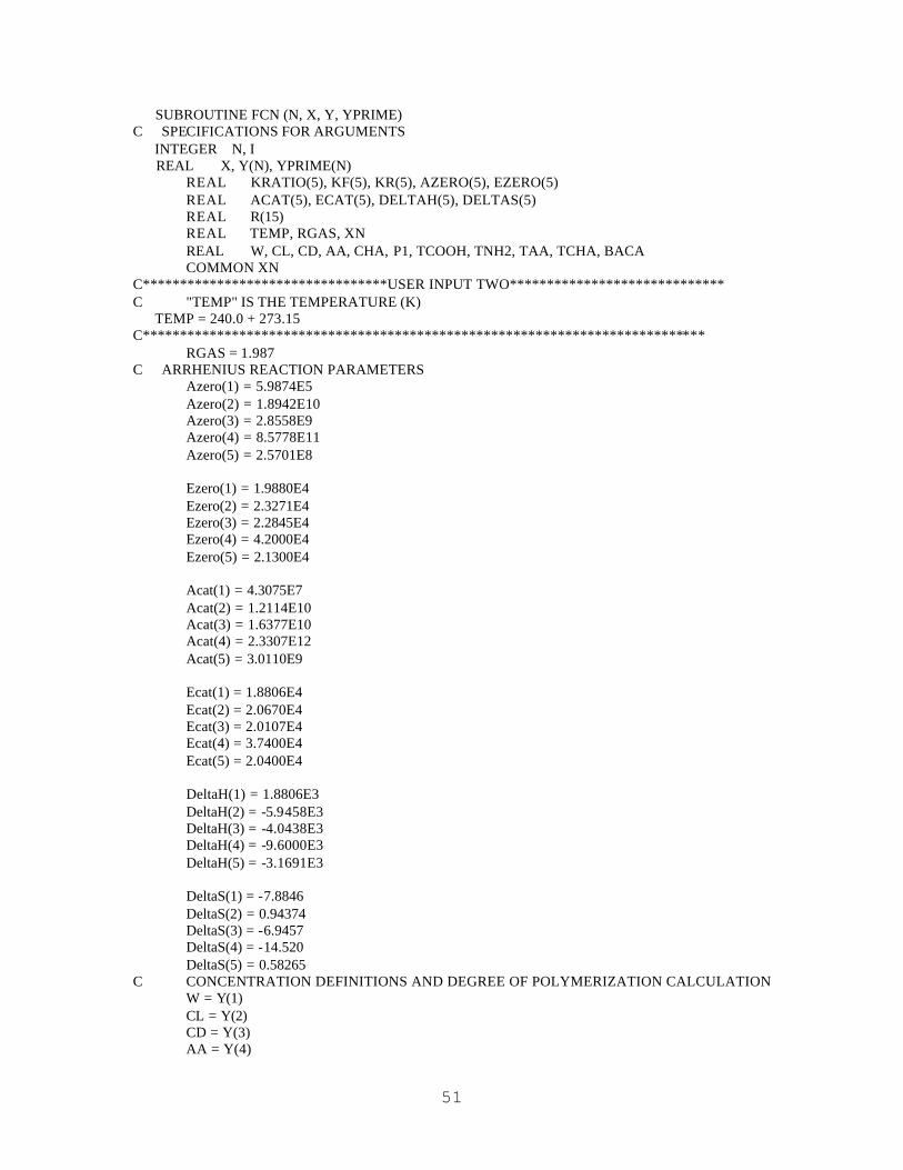
51
SUBROUTINE FCN (N, X, Y, YPRIME) C SPECIFICATIONS FOR ARGUMENTS INTEGER N, I REAL X, Y(N), YPRIME(N) REAL KRATIO(5), KF(5), KR(5), AZERO(5), EZERO(5) REAL ACAT(5), ECAT(5), DELTAH(5), DELTAS(5) REAL R(15) REAL TEMP, RGAS, XN REAL W, CL, CD, AA, CHA, P1, TCOOH, TNH2, TAA, TCHA, BACA COMMON XN C*********************************USER INPUT TWO***************************** C "TEMP" IS THE TEMPERATURE (K) TEMP = 240.0 + 273.15 C**************************************************************************** RGAS = 1.987 C ARRHENIUS REACTION PARAMETERS Azero(1) = 5.9874E5 Azero(2) = 1.8942E10 Azero(3) = 2.8558E9 Azero(4) = 8.5778E11 Azero(5) = 2.5701E8 Ezero(1) = 1.9880E4 Ezero(2) = 2.3271E4 Ezero(3) = 2.2845E4 Ezero(4) = 4.2000E4 Ezero(5) = 2.1300E4 Acat(1) = 4.3075E7 Acat(2) = 1.2114E10 Acat(3) = 1.6377E10 Acat(4) = 2.3307E12 Acat(5) = 3.0110E9 Ecat(1) = 1.8806E4 Ecat(2) = 2.0670E4 Ecat(3) = 2.0107E4 Ecat(4) = 3.7400E4 Ecat(5) = 2.0400E4 DeltaH(1) = 1.8806E3 DeltaH(2) = -5.9458E3 DeltaH(3) = -4.0438E3 DeltaH(4) = -9.6000E3 DeltaH(5) = -3.1691E3 DeltaS(1) = -7.8846 DeltaS(2) = 0.94374 DeltaS(3) = -6.9457 DeltaS(4) = -14.520 DeltaS(5) = 0.58265 C CONCENTRATION DEFINITIONS AND DEGREE OF POLYMERIZATION CALCULATION W = Y(1) CL = Y(2) CD = Y(3) AA = Y(4)

52
CHA = Y(5) P1 = Y(6) BACA = Y(7) TNH2 = Y(8) TCOOH = Y(9) TAA = Y(10) TCHA = Y(11) XN = (BACA+TCOOH+TNH2+ACA)/(ACA+TNH2+TAA+1E-12) + 1E-12 C RATE CONSTANT CALCULATION DO I = 1, 5 Kratio(I) = Exp(DeltaS(I) / Rgas - DeltaH(I) / (Temp * Rgas)) Kf(I) = Azero(I) * Exp(-1.0 * Ezero(I) / (Rgas * Temp)) + Acat & (I) * (P1 + TCOOH + AA) * Exp(-1.0 * Ecat(I) / (Rgas * Temp)) Kr(I) = Kf(I) / Kratio(I) END DO C REACTION RATES FOR EACH EQUILIBRIUM REACTION R(1) = KF(1)*CL*W - KR(1)*P1 R(2) = KF(2)*P1**2 - KR(2)*P1*W R(3) = KF(2)*P1*TCOOH - KR(2)*W*(TCOOH-P1-TAA/(XN**2)) R(4) = KF(2)*TNH2*P1 - KR(2)*W*(TNH2-P1-TCHA/(XN**2)) R(5) = KF(2)*TNH2*TCOOH - KR(2)*W*(BACA-TNH2-TAA+P1+2*TCHA/ & (XN**2)) R(6) = KF(3)*P1*CL - KR(3)*P1 R(7) = KF(3)*TNH2*CL - KR(3)*(TNH2-P1-TCHA/(XN**2)) R(8) = KF(4)*CD*W - KR(4)*P1 R(9) = KF(5)*P1*CD - KR(5)*P1 R(10) = KF(5)*TNH2*CD - KR(5)*(TNH2-2.0*P1-2.0*TCHA/(XN**2)) R(11) = KF(2)*AA*P1 - KR(2)*W*TAA/(XN**2) R(12) = KF(2)*AA*TNH2 - KR(2)*W*TAA*(1-1/(XN**2)) R(13) = KF(3)*CHA*CL - KR(3)*TCHA/(XN**2) R(14) = KF(2)*CHA*P1 - KR(2)*W*TCHA/(XN**2) R(15) = KF(2)*CHA*TCOOH - KR(2)*W*TCHA*(1-1/(XN**2)) C SPECIES BALANCES (O.D.E. SET) YPRIME(1) = R(2)+R(3)+R(4)+R(5)+R(11)+R(12)+R(14)+R(15) & - (R(1)+R(8)) YPRIME(2) = -1.0*(R(1)+R(6)+R(7)+R(13)) YPRIME(3) = -1.0*(R(8)+R(9)+R(10)) YPRIME(4) = -1.0*(R(11)+R(12)) YPRIME(5) = -1.0*(R(13)+R(14)+R(15)) YPRIME(6) = R(1) - (2.0*R(2)+R(3)+R(4)+R(6)+R(9)+R(11)+R(14)) YPRIME(7) = R(3)+R(4)+2.0*R(5)+R(7)+R(9)+2.0*R(10)+R(12)+R(15) YPRIME(8) = R(2)+R(6)+R(8)+R(9)+R(13)+R(14) - (R(5)+R(12)) YPRIME(9) = R(2)+R(6)+R(8)+R(9)+R(11) - (R(5)+R(15)) YPRIME(10) = R(11) + R(12) YPRIME(11) = R(13) + R(14) + R(15) RETURN END C***************************************************************************** SUBROUTINE FCNJ (N, X, Y, DYPDY) C SPECIFICATIONS FOR ARGUMENTS INTEGER N REAL X, Y(N), DYPDY(N,*) C THIS SUBROUTINE IS NEVER CALLED RETURN END

53
3 Phase Equilibrium in Nylon-6 Polymerizations46
In Chapter 2, we developed the basis for simulating the hydrolytic polymerization of
nylon-6: the reaction set. Reaction takes place in the liquid phase. Our task for this
chapter is to consider the central problem of the distribution of species when liquid and
vapor phases are present.
This chapter presents a thermodynamically consistent model for the phase equilibrium of
water/caprolactam/nylon-6 mixtures, based on the POLYNRTL (polymer non-random
two-liquid) activity-coefficient model. Our model predicts phase equilibrium for any
binary or ternary mixture containing water, ε-caprolactam, and nylon-6 at industrially
relevant temperatures and pressures with an average error of 1%. This chapter also
demonstrates its application to simulate industrial production of nylon-6. Prior literature
makes simplifying assumptions about liquid phase (molten polymer) activities of water
and ε-caprolactam; these assumptions are shown to be unrealistic.
Chapter organization is below:
• 3.1 – Introduction to nylon-6 production and simulation
• 3.2 – Literature review covering simulation technology for kinetics and phase
equilibrium, and phase-equilibrium data for the system water/caprolactam/nylon-6
• 3.3 – Methodology for analyzing and characterizing the phase-equilibrium of
water/caprolactam/nylon-6 mixtures
• 3.4 – Results of analysis
• 3.5 – Validation of binary interaction parameter set
• 3.6 – Application of the phase-equilibrium model to describe manufacturing trains
• 3.7 – Conclusions
46 Adapted from a manuscript submitted to Industrial and Engineering Chemistry Research (coauthors are
Neeraj P. Khare, Y. A. Liu, Thomas N. Williams , and Chau-Chyun Chen)

54
3.1 Introduction
Considering the economic scale of nylon-6 production (reviewed in Chapter 2), it is not
surprising that a number of polymerization models based on first principles have
appeared47,48,49,50,51. These models attempt to apply knowledge of kinetics, physical and
thermodynamic properties, mass and energy transport, and phase equilibrium to simulate
a manufacturing process. We can apply an accurate model to improve or maintain
product quality and increase production rate.
This chapter addresses inaccuracies in phase equilibrium that limit the accuracy of these
existing models. In particular, we describe commercial nylon-6 manufacturing
technologies to demonstrate the critical impact of phase equilibrium. We then outline
prior simulation studies that seek to understand and optimize these processes and their
deficiencies. Lastly, we discuss current problems facing the simulation of nylon-6 phase
equilibrium, and show how to address these problems.
3.1.1 Commercial Nylon-6 Manufacturing Processes
Figure 3.1 depicts a conventional nylon-6 production scheme.
47 Giori, C., and B. T. Hayes, “Hydrolytic Polymerization of Caprolactam. I. Hydrolysis –
Polycondensation Kinetics,” Journal of Polymer Science: Part A-1, 8, pp. 335-349 (1970). 48 Agrawal, A. K., K. Devika, and T. Manabe, “Simulation of Hydrolytic Polymerization of Nylon-6 in
Industrial Reactors: Part I. Mono-Acid-Stabilized Systems in VK Tube Reactors,” Industrial and
Engineering Chemistry Research, 40, pp. 2563-2572 (2001). 49 Gupta, S. K., D. Kunzru, A. Kumar, and K. K. Agarwal, “Simulation of Nylon-6 Polymerization in
Tubular Reactors with Recycle,” Journal of Applied Polymer Science, 28, pp. 1625-1640 (1983). 50 Amon, M., and C. D. Denson, “Simplified Analysis of the Performance of Wiped-Film Polycondensation
Reactors,” Industrial and Engineering Fundamentals, 19, pp. 415-420 (1980). 51 Gupta, A., S. K. Gupta, K. S. Ghandi, M. H. Mehta, M. R. Padh, A. V. Soni, and B. V. Ankleswaria,
“Modeling of Hydrolytic Polymerization in a Semi-Batch Nylon-6 Reactor,” Chemical Engineering
Communications, 113, pp. 63-89 (1992).

55
Polymerization Pelletizing LeachingAnd Drying
MonomerRecovery
Feed
Waste
ResinPolymerization Pelletizing LeachingAnd Drying
MonomerRecovery
Feed
Waste
Resin
Figure 3.1. A block diagram of a conventional nylon-6 polymerization process.
The reactor feed typically contains fresh caprolactam monomer, recycled monomer,
water, and desired additives52, such as chain-terminating agents, fire-retarding agents, and
delustrants. The reactor section hydrolyzes the monomer, converts it to polymer, and
builds the polymer molecular weight.
As the molten polymer is in equilibrium with water and monomer, the by-product water
must be removed by vaporization to increase the molecular weight. However,
vaporization of the water may also remove a significant amount of caprolactam, which is
recovered and recycled.
In conventional processes, the polymer is then pelletized, and leached with hot water to
remove low-molecular-weight extractables, such as residual monomer and cyclic
oligomers. The polymer is then dried and shipped elsewhere, or used directly to spin
fibers53.
52 Twilley, I. C., D. W. H. Roth, and R. A. Lofquist, “Process for the Production of Nylon-6,” United States
Patent #3,558,567 , Allied Chemical Corporation (1971). 53 Yates, S. L., C. J. Cole, A. H. Wiesner, and J. W. Wagner, “Two-Stage Hydrolysis Process for the
Preparation of Nylon-6,” United States Patent #4,310,659 , Allied Chemical Corporation (1982).

56
By contrast, in direct melt processes, the extraction and drying steps are avoided by
devolatilizing the polymer of unreacted monomer. Molten polymer can then be fed
directly to spinning or pelletizing. However, melt polymers are typically modified
(terminated with monofunctional amines and carboxylic acids) to limit the molecular
weight produced at the low levels of water achieved when removing unreacted
caprolactam. Therefore, direct melt processes have a limited product range compared
with conventional processes.
Within these two process variants, i.e., conventional and direct melt, a number of
commercial technologies are available to polymerize caprolactam. These technologies
include batch, bubble-gas kettle, melt (terminated and unterminated resins), traditional
VK (Vereinfacht Kontinuierliches), and solid-state processes. Even the depolymerization
of nylon-6 to recover caprolactam is practiced on a commercial scale 54. Table 3.1
summarizes these major technologies along with their approximate temperature and
pressure conditions.
54 http://www.oit.doe.gov/chemicals/pdfs/nylon.pdf (accessed September 2002)
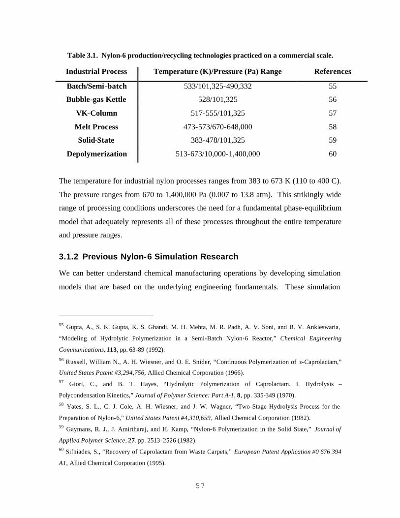
57
Table 3.1. Nylon-6 production/recycling technologies practiced on a commercial scale.
Industrial Process Temperature (K)/Pressure (Pa) Range References
Batch/Semi-batch 533/101,325-490,332 55
Bubble-gas Kettle 528/101,325 56
VK-Column 517-555/101,325 57
Melt Process 473-573/670-648,000 58
Solid-State 383-478/101,325 59
Depolymerization 513-673/10,000-1,400,000 60
The temperature for industrial nylon processes ranges from 383 to 673 K (110 to 400 C).
The pressure ranges from 670 to 1,400,000 Pa (0.007 to 13.8 atm). This strikingly wide
range of processing conditions underscores the need for a fundamental phase-equilibrium
model that adequately represents all of these processes throughout the entire temperature
and pressure ranges.
3.1.2 Previous Nylon-6 Simulation Research
We can better understand chemical manufacturing operations by developing simulation
models that are based on the underlying engineering fundamentals. These simulation
55 Gupta, A., S. K. Gupta, K. S. Ghandi, M. H. Mehta, M. R. Padh, A. V. Soni, and B. V. Ankleswaria,
“Modeling of Hydrolytic Polymerization in a Semi-Batch Nylon-6 Reactor,” Chemical Engineering
Communications, 113, pp. 63-89 (1992). 56 Russell, William N., A. H. Wiesner, and O. E. Snider, “Continuous Polymerization of ε-Caprolactam,”
United States Patent #3,294,756, Allied Chemical Corporation (1966). 57 Giori, C., and B. T. Hayes, “Hydrolytic Polymerization of Caprolactam. I. Hydrolysis –
Polycondensation Kinetics,” Journal of Polymer Science: Part A-1, 8, pp. 335-349 (1970). 58 Yates, S. L., C. J. Cole, A. H. Wiesner, and J. W. Wagner, “Two-Stage Hydrolysis Process for the
Preparation of Nylon-6,” United States Patent #4,310,659 , Allied Chemical Corporation (1982). 59 Gaymans, R. J., J. Amirtharaj, and H. Kamp, “Nylon-6 Polymerization in the Solid State,” Journal of
Applied Polymer Science, 27, pp. 2513-2526 (1982). 60 Sifniades, S., “Recovery of Caprolactam from Waste Carpets,” European Patent Application #0 676 394
A1, Allied Chemical Corporation (1995).

58
models can be used in a variety of beneficial ways; they speed up process development
and optimization, and can facilitate new product development.
Researchers who recognized the value of simulation began publishing models of nylon-6
polymerization in the 1970’s, with Giori and Hayes61 being one of the first. Initial
models for most commercial nylon polymerization technologies have now been
documented, including VK column62, plug-flow63, wiped-film64, and semi-batch
reactors65.
In modeling any multi-phase chemical manufacturing process, it is important to properly
model the phase equilibrium of the process66. Specifically, we must pay particular
attention to phase equilibrium when modeling nylon polymerizations. This is because the
water concentration in the liquid phase is the overwhelming factor in determining product
characteristics, such as production rate and molecular weight67. Furthermore, properly
representing the thermodynamics is the basis for fundamentally modeling mass-transfer
resistances in step-growth finishing reactors. If we cannot adequately model phase
61 Giori, C., and B. T. Hayes, “Hydrolytic Polymerization of Caprolactam. I. Hydrolysis –
Polycondensation Kinetics,” Journal of Polymer Science: Part A-1, 8, pp. 335-349 (1970). 62 Agrawal, A. K., K. Devika, and T. Manabe, “Simulation of Hydrolytic Polymerization of Nylon-6 in
Industrial Reactors: Part I. Mono-Acid-Stabilized Systems in VK Tube Reactors,” Industrial and
Engineering Chemistry Research, 40, pp. 2563-2572 (2001). 63 Gupta, S. K., D. Kunzru, A. Kumar, and K. K. Agarwal, “Simulation of Nylon-6 Polymerization in
Tubular Reactors with Recycle,” Journal of Applied Polymer Science, 28, pp. 1625-1640 (1983). 64 Amon, M., and C. D. Denson, “Simplified Analysis of the Performance of Wiped-Film Polycondensation
Reactors,” Industrial and Engineering Fundamentals, 19, pp. 415-420 (1980). 65 Gupta, A., S. K. Gupta, K. S. Ghandi, M. H. Mehta, M. R. Padh, A. V. Soni, and B. V. Ankleswaria,
“Modeling of Hydrolytic Polymerization in a Semi-Batch Nylon-6 Reactor,” Chemical Engineering
Communications, 113, pp. 63-89 (1992). 66 Bokis, C. P., H. Orbey, and C. C. Chen, “Properly Model Polymer Processes,” Chemical Engineering
Progress, 95(4), pp. 39-52 (1999). 67 Gupta, A., S. K. Gupta, K. S. Ghandi, M. H. Mehta, M. R. Padh, A. V. Soni, and B. V. Ankleswaria,
“Modeling of Hydrolytic Polymerization in a Semi-Batch Nylon-6 Reactor,” Chemical Engineering
Communications, 113, pp. 63-89 (1992).

59
equilibrium, then we will not be able to properly diagnose the appearance of significant
mass-transfer limitations or calculate interfacial equilibrium compositions.
While it is clear that properly modeling the phase equilibrium in nylon polymerizations is
important, it is unfortunate that virtually no nylon-6 model in the literature contains an
accurate, fundamental thermodynamic model. This is because there is considerable
uncertainty in the phase-equilibrium data themselves68. A possible exception is the
modeling study by Loth et al.69; however, they give no details regarding their phase-
equilibrium model.
Experimental phase-equilibrium measurements are difficult to make because the
water/caprolactam/nylon-6 system is reactive. Furthermore, the mixture
water/caprolactam is wide-boiling, with the normal boiling point of caprolactam above
260 °C. Characterizing this system and analyzing the resulting data requires a deep
understanding of the underlying kinetics and thermodynamics.
In an ideal world, we would have many sets of thermodynamically consistent phase-
equilibrium data for water/caprolactam, water/nylon-6, and caprolactam/nylon-6. These
data would cover a wide range of temperatures and pressures. Unfortunately, we suffer
from a lack of data, and the literature data that we do have are inconsistent.
3.1.3 Objectives of Current Study
We develop a thermodynamically consistent model for nylon-6 phase equilibrium using
the scarce and inconsistent literature data. This development involves characterizing the
binary interactions between caprolactam, water, and nylon-6 (Figure 3.2).
68 Gupta, A., S. K. Gupta, K. S. Ghandi, M. H. Mehta, M. R. Padh, A. V. Soni, and B. V. Ankleswaria,
“Modeling of Hydrolytic Polymerization in a Semi-Batch Nylon-6 Reactor,” Chemical Engineering
Communications, 113, pp. 63-89 (1992). 69 Loth, W., J. Vonend, U. Lehnen, G. Kory, and K. D. Hungenberg, “Simulation of the Entire Process for
the Development and Optimization of Polymer Process Concepts,” DECHEMA Monographs, 134, pp. 545-
556 (1998).
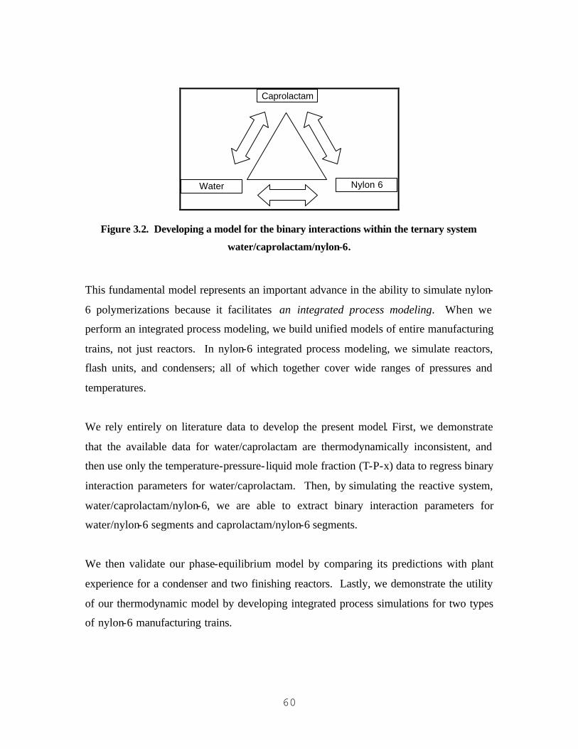
60
Caprolactam
Water Nylon 6
Figure 3.2. Developing a model for the binary interactions within the ternary system
water/caprolactam/nylon-6.
This fundamental model represents an important advance in the ability to simulate nylon-
6 polymerizations because it facilitates an integrated process modeling. When we
perform an integrated process modeling, we build unified models of entire manufacturing
trains, not just reactors. In nylon-6 integrated process modeling, we simulate reactors,
flash units, and condensers; all of which together cover wide ranges of pressures and
temperatures.
We rely entirely on literature data to develop the present model. First, we demonstrate
that the available data for water/caprolactam are thermodynamically inconsistent, and
then use only the temperature-pressure- liquid mole fraction (T-P-x) data to regress binary
interaction parameters for water/caprolactam. Then, by simulating the reactive system,
water/caprolactam/nylon-6, we are able to extract binary interaction parameters for
water/nylon-6 segments and caprolactam/nylon-6 segments.
We then validate our phase-equilibrium model by comparing its predictions with plant
experience for a condenser and two finishing reactors. Lastly, we demonstrate the utility
of our thermodynamic model by developing integrated process simulations for two types
of nylon-6 manufacturing trains.

61
3.2 Literature Review
We split our literature review into three sections: nylon-6 polymerization kinetics, phase-
equilibrium modeling, and water/caprolactam/nylon-6 phase-equilibrium data from the
literature. We report nylon-6 polymerization kinetics for two reasons. First, we simulate
the reactive system to obtain the binary interaction parameters for water/nylon-6
segments and caprolactam/nylon-6 segments. Second, we use the existing kinetic model,
along with our thermodynamic and mass-transfer models, to build integrated models for
commercial nylon-6 processes.
3.2.1 Nylon-6 Polymerization Kinetics
Arai et al.70 have presented the accepted standard regarding the chemistry and kinetics of
the hydrolytic polymerization of ε-caprolactam. Their reaction mechanism includes the
ring opening of caprolactam (CL), polycondensation, polyaddition of caprolactam, ring
opening of cyclic dimer (CD), and the polyaddition of cyclic dimer. Table 3.2 lists these
five equilibrium reactions.
Table 3.2. Nylon-6 polymerization reaction mechanisms.
Reaction Name Equilibrium Reaction
Ring opening of
caprolactam
1
1
k
2k '
H O CL ACA+ �
Polycondensation ( ) ( )2
2
k
2n n+1k 'ACA ACA ACA H O+ +�
Polyaddition of
caprolactam ( ) ( )
3
3
k
n n+1k 'CL ACA ACA+ �
Ring opening of
cyclic dimer
4
4
k
2k '
H O CD 2ACA+ �
Polyaddition of cyclic ( ) ( )5
5
k
n n+2k 'CD ACA ACA+ �
70 Arai, Y., K. Tai, H. Teranishi, and T. Tagawa, “Kinetics of Hydrolytic Polymerization of ε-Caprolactam:
3. Formation of Cyclic Dimer,” Polymer, 22, pp. 273-277 (1981).

62
dimer
*ACA is aminocaproic acid, (ACA)n is nylon-6 with a degree of polymerization n.
Table 3.3 gives the accompanying rate constants ki, again from Arai et al19.
Table 3.3. Rate constants for the equilibrium reactions in Table 3.2.
Rate constant expression [ ]0
0 exp expc
ci ii i i
E Ek A A T COOH
RT RT
= − + − −
Equilibrium constant
expression exp
'
iii
ii
HSk TKk R
∆ ∆ − = =
i 0
kg/mol-siA
0
J/moliE
2 2kg /mol -s
ciA
J/mol
ciE
J/moliH∆
J/mol-K
iS∆
1 1.66E+02 8.32E+04 1.20E+04 7.87E+04 8.03E+03 -33.01
2 5.26E+06 9.74E+04 3.37E+06 8.65E+04 -
2.49E+04 3.951
3 7.93E+05 9.56E+04 4.55E+06 8.42E+04 -
1.69E+04 -29.08
4 2.38E+08 1.76E+05 6.47E+08 1.57E+05 -
4.02E+04 -60.79
5 7.14E+04 8.92E+04 8.36E+05 8.54E+04 -
1.33E+04 2.439
We refer the reader to Arai et al.19 for the reaction-rate equations.
We add one more equilibrium reaction to this kinetic scheme: the termination reaction
with a monofunctional acid, such as acetic acid (HAC).

63
( ) ( )2
2
k
2n nxk 'HAC ACA ACA H O+ +� (3.1)
We assume that this reaction follows the same kinetics as the polycondensation reaction,
as in reference 47.
We ignore the analysis of cyclic oligomers higher than dimers for sake of simplicity.
3.2.2 Polymer Equilibrium
3.2.2.1 Previous Attempts to Develop a Phase-Equilibrium Model for
Water/Caprolactam/Nylon-6
Researchers typically use one of three phase-equilibrium models in simulating nylon-6
polymerizations: the Jacobs/Schweigman model71, the Fukumoto model72, or the Tai et
al.13 model. These models only predict water concentrations in reacting mixtures of
water, caprolactam, and nylon-6.
The Jacobs/Schweigman model is the most simplistic of the three models. It consists of
an empiricism based on experimental equilibrium data for a VK column reactor. The
model predicts the concentration of water [W] as a function of temperature T:
( )1.76 0.006 °Cmol
[ ]kg 1.8
TW
− =
(3.2)
71 Jacobs, H., and C. Schweigman, “Mathematical Model for the Polymerization of Caprolactam to Nylon-
6,” Proceedings of the Fifth European/Second International Symposium on Chemical Reaction
Engineering, Amsterdam, May 2-4, pp. B7.1-26 (1972). 72 Fukumoto, O., “Equilibria Between Polycapramide and Water. I.,” Journal of Polymer Science, XXII,
pp. 263-270 (1956).
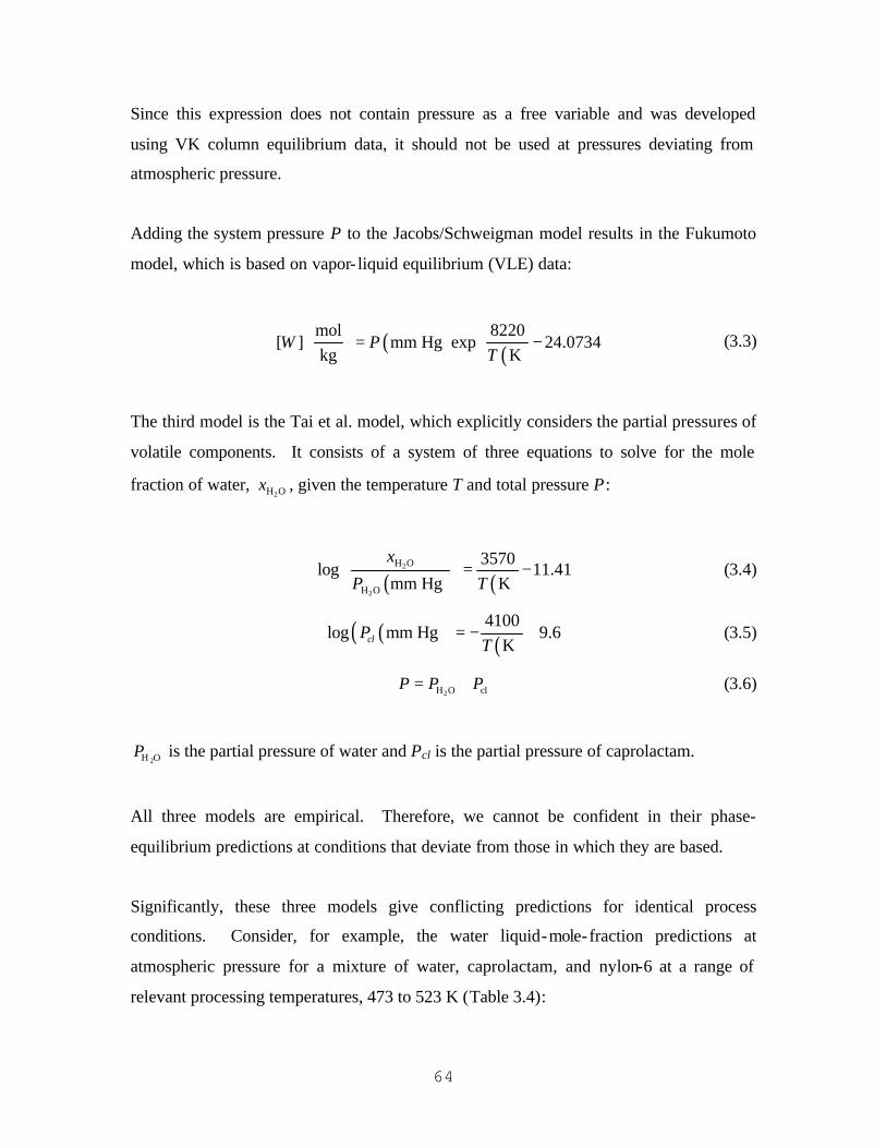
64
Since this expression does not contain pressure as a free variable and was developed
using VK column equilibrium data, it should not be used at pressures deviating from
atmospheric pressure.
Adding the system pressure P to the Jacobs/Schweigman model results in the Fukumoto
model, which is based on vapor- liquid equilibrium (VLE) data:
( ) ( )mol 8220
[ ] mm Hg exp 24.0734kg K
W PT
= −
(3.3)
The third model is the Tai et al. model, which explicitly considers the partial pressures of
volatile components. It consists of a system of three equations to solve for the mole
fraction of water, 2H Ox , given the temperature T and total pressure P:
( ) ( )
2
2
H O
H O
3570log 11.41
mm Hg K
x
P T
= −
(3.4)
( )( ) ( )4100
log mm Hg 9.6KclP
T= − + (3.5)
2H O clP P P= + (3.6)
2H OP is the partial pressure of water and Pcl is the partial pressure of caprolactam.
All three models are empirical. Therefore, we cannot be confident in their phase-
equilibrium predictions at conditions that deviate from those in which they are based.
Significantly, these three models give conflicting predictions for identical process
conditions. Consider, for example, the water liquid-mole-fraction predictions at
atmospheric pressure for a mixture of water, caprolactam, and nylon-6 at a range of
relevant processing temperatures, 473 to 523 K (Table 3.4):

65
Table 3.4. Liquid-phase, water mole -fraction predictions at one atmosphere for the
Jacobs/Schweigman, Fukumoto, and Tai et al. phase-equilibrium models.
Temperature (K) Jacobs/Schweigman Fukumoto Tai et al.
473 0.006 0.017 0.103
493 0.004 0.008 0.050
513 0.003 0.004 0.025
533 0.002 0.002 0.013
The Fukumoto model predic ts mole fractions that are about twice those of the
Jacobs/Schweigman predictions. Furthermore, the Tai et al. model predicts mole
fractions that are an order of magnitude higher than both models. This difference casts
considerable doubt on the validity of at least two of these models.
3.2.2.2 POLYNRTL Model
Bokis et al.17 give an excellent description of how to choose an appropriate
thermodynamic equilibrium model when simulating polymer processes. They suggest
using activity-coefficient models, instead of equations of state, for processes that involve
low-to-moderate pressures (pressure < 1E+6 Pa) and/or nonideal components (e.g., polar
compounds such as alcohols, water, and ketones).
Furthermore, they state that the polymer-non-random-two-liquid (POLYNRTL) activity-
coefficient model73 has the following advantages over the Flory-Huggins74,75 and
universal quasi-chemical functional group (UNIFAC)76 activity-coefficient models:
73 Chen, C. C., “A Segment-based Local Composition Model for the Gibbs Energy of Polymer Solutions,”
Fluid Phase Equilibria, 83, pp. 301-312 (1993). 74 Flory, P. J., “Thermodynamics of High Polymer Solutions,” Journal of Chemical Physics, 10, pp. 51-61
(1942). 75 Huggins, M. L., “Some Properties of Solutions of Long-Chain Compounds,” Journal of Physical
Chemistry, 46, pp. 151-158 (1942). 76 Fredenslund, A., R. L. Jones, and J. M. Prausnitz, “Group Contribution Estimation of Activity
Coefficients in Nonideal Liquid Mixtures,” AIChE Journal, 21, pp. 1086-1099 (1975).
66
1. POLYNRTL covers large ranges of temperatures and compositions accurately.
2. POLYNRTL takes advantage of the already existing database of NRTL binary
interaction parameters.
Based on these suggestions, we choose to model nylon-6 phase equilibrium using the
POLYNRTL property method. This method uses: (1) the polymer NRTL activity-
coefficient model for the liquid phases; (2) the Redlich-Kwong77 equation of state for the
vapor phase; (3) the van Krevelen78 model for the liquid properties (enthalpy, entropy,
Gibbs free energy, heat capacity, and molar volume); and (4) Henry’s law for any
supercritical components.
The POLYNRTL activity-coefficient model combines the traditional NRTL model with
the Flory-Huggins description for configurational entropy. It essentially calculates the
Gibbs free energy of mixing in a polymer solution as the sum of two contributions: (1)
the entropy of mixing from Flory-Huggins (FH) activity-coefficient model; and (2) the
enthalpy of mixing from NRTL activity-coefficient model79. These activity coefficients
include binary parameters to model the interactions between two components.
POLYNRTL represents the temperature dependence of the binary interaction parameters
(τij) by Eq. (3.7):
lnijij ij ij
ba c T
Tτ = + + (3.7)
We set the non-randomness factor αij to 0.3, as suggested by Prausnitz et al. 80
77 Redlich, O., and J. N. S. Kwong, “On the Thermodynamics of Solutions. V. An Equation of State.
Fugacities of Gaseous Solutions,” Chemical Reviews, 44: 233-244, 1949. 78 Van Krevelen, D. W., Properties of Polymers, Elsevier, New York, pp. 1-875, 1990. 79 Renon, H., and J. M. Prausnitz, “Local Compositions in Thermodynamic Excess Functions for Liquid
Mixtures,” AIChE Journal, 14, pp. 135-144 (1968). 80 Prausnitz, J. M., R. N. Lichtenthaler, and E. G. de Azevedo, Molecular Thermodynamics of Fluid-Phase
Equilibrium, 3 rd ed., Prentice Hall, New Jersey, p. 261 (1999).
67
Therefore, we model binary interactions in equilibrium mixtures by specifying the
coefficients aij through cij. We typically regress equilibrium data or use a predictive
model, such as UNIFAC, to obtain the values of these parameters.
3.2.3 Equilibrium Data for Water/Caprolactam/Nylon-6
There are two sources of phase-equilibrium data that we use for regression. The first
source characterizes the binary interactions between water and caprolactam. The second
characterizes the interactions in the reactive, ternary system nylon-6/caprolactam/water.
All of the data sets appear in the Supporting Information Sec. 3.8.
Manczinger and Tettamanti81 give four sets of low-pressure, isobaric phase-equilibrium
data for the binary water/caprolactam. Table 3.14 through Table 3.17 show their data.
Giori and Hayes82 present one set of isothermal phase-equilibrium data for the ternary
system water/caprolactam/nylon-6. They carry out nylon-6 polymerizations at 543 K in a
laboratory reactor and characterize the resulting phase equilibrium. Table 3.18 shows
their experimental data.
3.3 Methodology
We first characterize the binary interactions between water and caprolactam using the
first four data sets30. We then simulate the Giori and Hayes experiments31 to quantify the
binary interactions between water/nylon-6 and caprolactam/nylon-6.
3.3.1 Characterizing the Phase Equilibrium of Water/Caprolactam
Here, we explain how to obtain the binary parameters for water/caprolactam. Our
handling of the data consists of testing the data for thermodynamic consistency. We use
81 Maczinger, J., and K. Tettamanti, “Phase Equilibrium of the System Caprolactam/Water,” Periodica
Polytechnica, 10, 183 (1966). 82 Giori, C., and B. T. Hayes, “Hydrolytic Polymerization of Caprolactam. II. Vapor-Liquid Equilibrium,”
Journal of Polymer Science: Part A-1, 8, pp. 351-358 (1970).

68
two consistency tests for our isobaric data sets: a Van Ness et al. test83 and a Wisniak
test84. The Wisniak test can be used in a point or area mode; however, we use only the
point test because of the difficulty in accurately computing integrals of “functions” of our
experimental data.
3.3.1.1 Consistency Test One: Van Ness et al. Test
In this test, we first obtain a redundant data set comprised of temperature, pressure, liquid
mole fraction, and vapor mole fraction measurements (T-P-xy). We then regress only the
T-P-x data. After regressing these data, we are able to predict the original pressure data
(using T-x data) and vapor mole fraction data (using T-P-x data). Consistency test one
comes by examining the extent of corroboration between the measured and predicted
vapor mole fractions. This test is an indirect application of the Gibbs-Duhem equation
since the POLYNRTL model obeys the Gibbs-Duhem equation.
The fundamental phase-equilibrium relation for this analysis is:
( ) ( ) ( ), expsat sii i i i i i i
vy P x x T P T P P
RTφ γ = −
(3.8)
We compute the activity coefficient iγ using the POLYNRTL model; it is a function of
the liquid composition xi and temperature T. satiP is the vapor pressure, which we
compute using an Antoine form:
exp ln iEsat ii i i i
BP A C T DT
T = + + +
(3.9)
83 Van Ness, H. C., S. M. Byer, and R. E. Gibbs, “Vapor-Liquid Equilibrium: Part 1. An Appraisal of Data
Reduction Methods,” AIChE Journal, 19, pp. 238-244 (1973). 84 Wisniak, J., “A New Test for the Thermodynamic Consistency of Vapor-Liquid Equilibrium,” Industrial
and Engineering Chemistry Research, 32, pp. 1531-1533 (1993).

69
We have neglected vapor-phase non-idealities (fugacity coefficient iφ equals one)
because most of the data are at vacuum conditions; however, one can easily estimate the
degree of vapor-phase non- ideality occurring at high pressures using the Redlich-Kwong
equation of state. Furthermore, the Poynting pressure correction is negligible
(exponential term is one).
We eliminate the need for vapor-composition data by summing Eq. (3.8) over all species;
for a binary system containing species i and j, we have:
( ) ( ) ( ) ( ), ,sat sati i i i j j j jP x x T P T x x T P Tγ γ= + (3.10)
Using the T-P-x data, we manipulate the six POLYNRTL binary interaction parameters
(aij – cij for water-caprolactam and caprolactam-water, Eq. (3.7)) to minimize the
following sum-of-squares error for each data point k:
2observed calculated
observedk k
k k
P PSSE
P −
=
∑ (3.11)
Once we have the binary interaction parameters, we predict the vapor composition using
the original T-P-x data and Eq. (3.8). Lastly, we compute the percent difference in vapor
mole-fraction data vs. prediction for each liquid-composition data point:
calculated observed
observedPercent Deviation 100%y y
y −
=
(3.12)
We plot the percent deviation vs. the liquid mole fraction to characterize the consistency
of the observed phase-equilibrium data.

70
3.3.1.2 Consistency Test Two: Wisniak Test
The second consistency test that we use, due to Wisniak, is based on the bubble-point
equation for mixtures and utilizes the Clausius-Clapeyron equation. It is fundamentally-
based and preferable to a combined Redlich-Kister85/Herington method86 for testing the
consistency of isobaric phase-equilibrium data.
For each data point i at system temperature Ti, we compute two functions Li and Wi:
k k ki i
T x sL T
s
° ∆ °= −
∆∑ (3.13)
( )lnk k
i i
x wW RT
s
γ −=
∆
∑ (3.14)
For every species k, at the system pressure, there is a pure-component boiling point kT ° ,
a liquid mole fraction xk, and entropy of vaporization ks∆ ° . In Eq. (3.14), s∆ is the
entropy of mixing of the mixture.
We compute the boiling temperature kT ° for each component k by setting the pressure to
the system pressure in Eq. (3.9) and then backing out the temperature.
We calculate the entropy of vaporization from the enthalpy of vaporization kh∆ ° :
2
, ,
,
1
k k
c k c k
T TB C DT T
kk
c kkk
k k
TA
Ths
T T
° °+ + °
− ∆ ° ∆ ° = =° °
(3.15)
85 Prausnitz, J. M., R. N. Lichtenthaler, and E. G. de Azevedo, Molecular Thermodynamics of Fluid-Phase
Equilibrium, 3 rd ed., Prentice Hall, New Jersey, p. 247 (1999). 86 Herington, E. F. G., “Tests for the Consistency of Experimental Isobaric Vapour-Liquid Equilibrium
Data,” Journal of the Petroleum Institute, 37, pp. 457-470 (1951).
71
The critical temperature Tc,k as well as the constants Ak through Dk are tabulated in
standard reference sources (such as AIChE data compilations 87) and differ for each
chemical species.
We find the activity coefficients from the experimental data using Eq. (3.16):
( )
ii sat
i i
y Px P T
γ = (3.16)
We compute the mixture entropy of vaporization for the mixture s∆ using the following
mixing rule:
k ks x s∆ = ∆ °∑ (3.17)
Lastly, we find the w term appearing in Eq. (3.14) using:
ln kk
k
yw x
x
=
∑ (3.18)
We perform the point test by computing the ratio of Li and Wi and plotting this as a
function of liquid mole fraction. Inconsistent data contains ratio values that are much
different than one and do not scatter randomly about one.
3.3.1.3 Determining Binary Interaction Parameters from Phase-
Equilibrium Data
The Van Ness et al. test effectively regresses binary interaction-parameters using T-P-x
data only. If the data are judged inconsistent, we assume that the vapor-phase
87 Daubert, T. E., and R. P. Danner, Physical and Thermodynamic Properties of Pure Chemicals. Data
Compilation. Vol. 1 , Hemisphere Publishing Corporation, New York, p. V-1 (1989).

72
composition data are bad88. This is because it is harder to accurately measure vapor
compositions than liquid compositions.
If the data are inconsistent and we throw out the vapor mole- fraction measurements, then
we have already obtained binary interaction parameters using the data that we are most
confident in (T-P-x data). However, if the data are consistent, then we can use all of the
data to compute activity coefficients (via Eq. (3.16)) and re-regress the binary interaction
parameters.
3.3.2 Characterizing the Ternary, Reactive System
Water/Caprolactam/Nylon-6
By completing the first step of this study, Sec. 3.3.1, we obtain the binary interaction
parameters for the system water/caprolactam. We then simulate the Giori and Hayes
experiments in order to characterize the binary interactions between water/nylon-6
segments and caprolactam/nylon-6 segments. We use a commercial simulation package,
POLYMERS PLUS by Aspen Technology, Inc., Cambridge, Massachusetts, to model the
batch step-growth polymerizations. However, our methodology is applicable in any
polymer process simulator.
We simulate a 0.000077-m3 (77 ml) reactor using the Arai et al. kinetic scheme and the
binary interaction parameters for water/caprolactam. We maintain a vapor- liquid system
throughout the polymerization. After reaction equilibrium is reached in the closed vessel,
we predict final liquid and vapor compositions, as well as the final pressure.
Since we have a relatively small amount of data, we must minimize the number of free
parameters in fitting the reaction data. We regress the bij parameters for water/nylon-6
segment interactions and caprolactam/nylon-6 segment interactions. We fix the aij and cij
parameters to zero.
88 Prausnitz, J. M., R. N. Lichtenthaler, and E. G. de Azevedo, Molecular Thermodynamics of Fluid-Phase
Equilibrium, 3 rd ed., Prentice Hall, New Jersey, p. 249 (1999).

73
We vary these four binary interaction parameters, one for each binary interaction, until
we match the outlet compositions and pressures from the data of Giori and Hayes. The
resulting binary interaction parameters characterize the systems, water/nylon-6 segments
and caprolactam/nylon-6 segments.
3.4 Results and Discussion
3.4.1 Binary Interaction Parameters for Water/Caprolactam
Table 3.5 contains the pertinent physical property constants for water and caprolactam,
found in Daubert and Danner36. We need these parameters to compute the vapor pressure
and enthalpy of vaporization.
Table 3.5. Physical property constants for water and caprolactam. The vapor pressure is
computed using Eq. (3.9), with units of Pa and temperature units of K. The enthalpy of
vaporization is computed using Eq. (3.15), with units of J/kmol and temperature units of K.
Constant Water Caprolactam
Vapor pressure
Ai 7.3649E+01 7.4172E+01
Bi -7.2582E+03 -1.0469E+04
Ci -7.3037E+00 -6.8944E+00
Di 4.1653E-06 1.2113E-18
Ei 2.0000E+00 6.0000E+00
Enthalpy of vaporization
Ai
5.2053E+07 8.3520E+07
Bi 3.1990E-01 3.7790E-01
Ci -2.1200E-01 0.0000E+00
Di 2.5795E-01 0.0000E+00
Critical temperature (K) 806.00 647.13
Figure 3.3 shows the results of the Van Ness et al. test for thermodynamic consistency: a
plot of the percent error in vapor mole fraction vs. liquid mole fraction for caprolactam.

74
-200%
0%
200%
400%
600%
800%
1000%
1200%
0 0.2 0.4 0.6 0.8 1
x CL
Err
or in
y C
L
Figure 3.3. Percent error in vapor mole fraction prediction vs. liquid mole fraction for
caprolactam for all data sets (Van Ness et al. test).
Consistent data show small, randomly-distributed errors around the x axis. Inconsistent
data give large, non-randomly distributed errors. It is clear from Figure 3.3 that all data
sets are inconsistent; this suggests that we should ignore vapor-phase measurements.
Similarly, for the Wisniak test, we show a ratio plot in Figure 3.4.
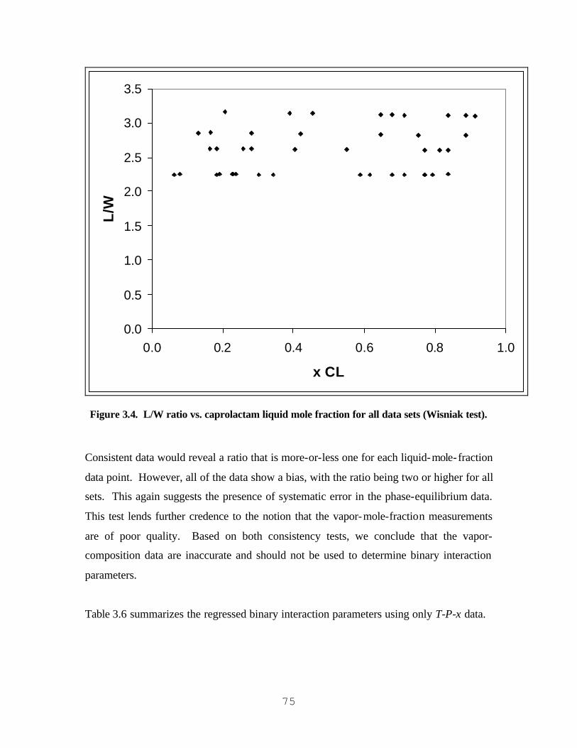
75
0.0
0.5
1.0
1.5
2.0
2.5
3.0
3.5
0.0 0.2 0.4 0.6 0.8 1.0
x CL
L/W
Figure 3.4. L/W ratio vs. caprolactam liquid mole fraction for all data sets (Wisniak test).
Consistent data would reveal a ratio that is more-or-less one for each liquid-mole-fraction
data point. However, all of the data show a bias, with the ratio being two or higher for all
sets. This again suggests the presence of systematic error in the phase-equilibrium data.
This test lends further credence to the notion that the vapor-mole-fraction measurements
are of poor quality. Based on both consistency tests, we conclude that the vapor-
composition data are inaccurate and should not be used to determine binary interaction
parameters.
Table 3.6 summarizes the regressed binary interaction parameters using only T-P-x data.

76
Table 3.6. Regression results for POLYNRTL binary interaction parameters for
water/caprolactam (based on T-P-x data only).
POLYNRTL Binary Interaction
Parameter Value (Temperature Units are K)
awater-cl -0.313
acl-water 0.628
bwater-cl -15.4
bcl-water -13.7
cwater-cl 0.0495
ccl-water -0.0898
Figure 3.5 shows the plot of the POLYNRTL parameters ijτ vs. temperature.
-0.1
-0.08
-0.06
-0.04
-0.02
0
0.02
0.04
0.06
0.08
0 50 100 150 200 250 300
Temperature (°C)
PO
LY
NR
TL
Tau
Tau (water-cl)Tau (cl-water)
Figure 3.5. Predicted value of the POLYNRTL binary parameter tau for
water/caprolactam and caprolactam/water.

77
The binary interaction parameter ijτ is not significantly different from zero over a wide
temperature range. This suggests that the energy of interaction does not largely differ
between unlike interactions vs. like interactions (i.e., near- ideal solution behavior).
We plot the experimental data vs. POLYNRTL model calculations for each of the four
isobars in Figure 3.6 through Figure 3.9.
0
50
100
150
200
250
300
0 0.2 0.4 0.6 0.8 1
Water Mole Fraction
Tem
per
atu
re (
°C)
Data - x waterData - y waterPOLYNRTL - x waterPOLYNRTL - y water
Figure 3.6. Water/caprolactam T-x-y diagram (101,325 Pa).

78
0
50
100
150
200
250
0 0.2 0.4 0.6 0.8 1
Water Mole Fraction
Tem
per
atu
re (
°C)
Data - x waterData - y waterPOLYNRTL - x waterPOLYNRTL - y water
Figure 3.7. Water/caprolactam T-x-y diagram (24,000 Pa).

79
0
20
40
60
80
100
120
140
160
180
200
0 0.2 0.4 0.6 0.8 1
Water Mole Fraction
Tem
per
atu
re (
°C)
Data - x waterData - y waterPOLYNRTL - x waterPOLYNRTL - y water
Figure 3.8. Water/caprolactam T-x-y diagram (10,700 Pa).

80
0
20
40
60
80
100
120
140
160
180
0 0.2 0.4 0.6 0.8 1
Water Mole Fraction
Tem
per
atu
re (
°C)
Data - x waterData - y waterPOLYNRTL - x waterPOLYNRTL - y water
Figure 3.9. Water/caprolactam T-x-y diagram (4,000 Pa).
The POLYNRTL model accurately correlates the phase-equilibrium data. Furthermore,
assuming ideal behavior in the vapor and liquid phases gives nearly identical predictions.
Therefore, we may safely neglect non-idealities in water/caprolactam solutions under
vacuum.
3.4.2 Binary Interaction Parameters for Water/Caprolactam/Nylon-6
With these binary interaction parameters, we turn to simulating the Giori and Hayes data.
We manipulate the second binary interaction parameters bij for small molecule/nylon-6
segment interactions. We obtain model predictions and compare them with the Giori and
Hayes data in Table 3.7.

81
Table 3.7. Comparison of model predictions with Giori and Hayes polymerization data.
Caprolactam liquid
mole fraction
Water liquid mole
fraction
Water vapor mole
fraction Total pressure (Pa)
Data
0.096 0.012 0.74 571,473
0.097 0.0249 0.85 974,203
0.099 0.0387 0.886 1,399,298
0.101 0.0515 0.89 1,826,890
0.106 0.065 0.91 2,156,196
Model Prediction
0.087 0.012 0.69 537,087
0.086 0.025 0.84 1,013,377
0.086 0.039 0.90 1,444,827
0.085 0.052 0.93 1,831,991
0.085 0.066 0.95 2,177,624
% Error
-9.38% 0.00% -6.76% -6.02%
-11.34% 0.40% -1.18% 4.02%
-13.13% 0.78% 1.58% 3.25%
-15.84% 0.97% 4.49% 0.28%
-19.81% 1.54% 4.40% 0.99%
The binary interaction parameters are water-nylon 6 segment nylon 6 segment-water297/ 601b b= = − and
cl-nylon 6 segment nylon 6 segment-cl265/ 207b b= = (temperature units in K).
The average model prediction error for water compositions is 0.74%. Note that we are
most interested in these compositions since they significantly impact final polymer
properties, such as polymer molecular weight and conversion. The model under-predicts
the final caprolactam liquid composition by about 13.9%. The average error for the final
pressure prediction is -0.51%.
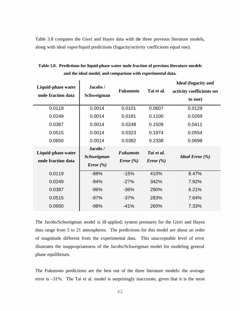
82
Table 3.8 compares the Giori and Hayes data with the three previous literature models,
along with ideal vapor/liquid predictions (fugacity/activity coefficients equal one).
Table 3.8. Predictions for liquid-phase water mole fraction of previous literature models
and the ideal model, and comparison with experimental data.
Liquid-phase water
mole fraction data
Jacobs /
Schweigman Fukumoto Tai et al.
Ideal (fugacity and
activity coefficients set
to one)
0.0119 0.0014 0.0101 0.0607 0.0129
0.0249 0.0014 0.0181 0.1100 0.0269
0.0387 0.0014 0.0248 0.1509 0.0411
0.0515 0.0014 0.0323 0.1974 0.0554
0.0650 0.0014 0.0382 0.2338 0.0698
Liquid-phase water
mole fraction data
Jacobs /
Schweigman
Error (%)
Fukumoto
Error (%)
Tai et al.
Error (%) Ideal Error (%)
0.0119 -88% -15% 410% 8.47%
0.0249 -94% -27% 342% 7.92%
0.0387 -96% -36% 290% 6.21%
0.0515 -97% -37% 283% 7.64%
0.0650 -98% -41% 260% 7.33%
The Jacobs/Schweigman model is ill-applied; system pressures for the Giori and Hayes
data range from 5 to 21 atmospheres. The predictions for this model are about an order
of magnitude different from the experimental data. This unacceptable level of error
illustrates the inappropriateness of the Jacobs/Schweigman model for modeling general
phase equilibrium.
The Fukumoto predictions are the best out of the three literature models: the average
error is –31%. The Tai et al. model is surprisingly inaccurate, given that it is the most

83
advanced out of the three. The average error of the Tai et al. model is 317%. Lastly,
neglecting non- ideality results in water liquid composition errors of 7.52%. Since water-
concentration terms in the kinetic expressions are proportional to water mole fractions in
the liquid phase, we can expect that this error would cause errors of ca. 8% when
computing reaction-rate terms. A likely explanation as to why ideal behavior
approximates the Giori and Hayes data is that the excess Gibbs energy of mixing is low
when the composition is at extreme values (polymer fraction is near zero or one).
By way of comparison, our new phase-equilibrium model generates an average prediction
error for the water liquid mole fraction of 1%. More importantly, it allows us to make
phase-equilibrium predictions in any binary or ternary mixture that primarily contains
water, caprolactam, and nylon-6 at any specified temperature and pressure. Table 3.9
contains our final binary interaction-parameter set.
Table 3.9. POLYNRTL binary interaction parameters for water/caprolactam/nylon-6
(temperature units are K).
Component i = Water Nylon-6 segment Nylon-6 segment
Component j = Cl Water Cl
aij -0.313 0 0
aji 0.628 0 0
bij -15.4 -601 207
bji -13.7 297 265
ci j 0.0495 0 0
cj i -0.0898 0 0
3.5 Validation of Regressed Binary Interaction Parameters
We consider two model predictions to be good indicators of the quality of our binary
interaction parameters: condenser performance and devolatization in finishing reactors.
Here, we perform exploratory simulations of a commercial condenser and two
commercial finishing reactors.

84
The feed contains a mixture of caprolactam and water. The condenser operates at a
temperature of 483 K and a pressure is 53,000 Pa. When we simulate the condenser as a
single flash unit, we get predictions for the liquid and vapor stream flow rates. Figure
3.10 compares our predictions with plant experience.
0
0.1
0.2
0.3
0.4
0.5
0.6
0.7
0.8
0.9
1
Vapor stream, cl Vapor stream,water
Liquid stream, cl Liquid stream,water
Mas
s F
low
Rat
e
Plant experienceModel prediction
Figure 3.10. Mass flow rates exiting condenser - model prediction vs. plant experience. All
values have been normalized using the largest flow rate.
The vapor-phase flow rates of caprolactam and water are predicted with an average error
of about 4%. The model under-predicts the liquid-phase component flow rates of
caprolactam and water by about 9%.
It is significant to note the split fractions: the data show that about 49% of the
caprolactam is vaporized, while 99% of the water is vaporized. Our phase-equilibrium

85
predictions nearly match the data, showing 53% for caprolactam vaporization and 99%
for water vaporization.
In our model of the first finishing reactor, we simulate a vapor- liquid plug-flow reactor,
with a feed stream containing 1 part by weight water, 77 parts caprolactam, and 423 parts
nylon-6. The molecular weight of the incoming polymer is 11.5 kg/mol. The reactor is
operating at ca. 520 K and 4,000 Pa with a residence time of 600 seconds11.
By way of validation, we are looking at the devolatization behavior of small molecules,
namely, caprolactam. From prior experience89, we know that devolatization of
caprolactam is mass-transfer limited. Therefore, if we ignore mass-transfer limitations in
the finishing reactor model, we should devolatize too much caprolactam and therefore
under-predict the mass fraction of caprolactam in the exiting melt stream.
Our model under-predicts the caprolactam mass fraction in the exit stream by 38%. This
shows that our phase-equilibrium calculations are reasonable. What would not be
reasonable is an equilibrium prediction for the caprolactam percentage that is actually
more than the mass-transfer limited case. Regarding the caprolactam mass percentage in
the exiting melt, the equilibrium case should always be lower than the mass-transfer-
limited case.
Now we simulate a second finishing reactor. Once again, we consider a vapor-liquid
plug-flow reactor, with a feed stream containing 1 part by weight water, 58 parts
caprolactam, and 356 parts nylon-6. The molecular weight of the incoming polymer is
9.8 kg/mol. This reactor is operating at ca. 523 K and 4,670 Pa with a residence time of
1,740 seconds11.
89 Nagasubramanian, K., and H. K. Reimschuessel, “Diffusion of Water and Caprolactam in Nylon-6
Melts,” Journal of Applied Polymer Science, 17, pp. 1663-1677 (1973).

86
Our model under-predicts the caprolactam mass fraction in the exit stream by 44%. This
again shows that our phase-equilibrium calculations are reasonable.
Regarding the finishing reactor studies, one may ask the following valid question: may
we approximate the error of the phase-equilibrium model from these results, as in the
condenser study? Unfortunately, this is not possible because we do not know to what
extent mass-transfer limitations are affecting the reactor performance. In other words, if
there is no mass-transfer limitation, the phase-equilibrium model is in error by –38 to
44%. If there is a strong mass-transfer limitation, then the phase-equilibrium model may
have large, little or no error.
3.6 Model Application
Previous attempts at nylon-6 integrated process modeling were hindered by the lack of a
fundamental thermodynamic phase-equilibrium model. For example, Reimschuessel and
Nagasubramanian90 simulated the molecular weight build in the finishing stage by first
“instantaneously” removing all water from the polymerization mass, while ignoring
caprolactam devolatization. There is no corresponding unit operation that can perform
this separation in an actual plant. Furthermore, this assumption has led Tirrell et al. 91 to
an unusual conclusion: that it is preferable to perform molecular weight build and
monomer conversion in a single reactor. To have adequate molecular weight build, we
need to enforce low water concentrations. However, to do this, we typically use severe
operating conditions, such as high vacuum in melt processes11, to remove most of the
water. In doing so, we cannot avoid losing a significant amount of the caprolactam to the
vapor phase. Therefore, equilibrium thermodynamics clearly suggests that it is
impractical to try to obtain both molecular weight build and monomer conversion in the
same reactor.
90 Nagasubramanian, K., and H. K. Reimschuessel, “Caprolactam Polymerization. Polymerization in
Backmix Flow Systems,” Journal of Applied Polymer Science, 16, pp. 929-934 (1972). 91 Tirrell, M. V., G. H. Pearson, R. A. Weiss, and R. L. Laurence, “An Analysis of Caprolactam
Polymerization,” Polymer Engineering and Science, 15, pp. 386-393 (1975).
87
Assuming instantaneous and complete water removal was necessary in the past because
researchers did not have access to a fundamental thermodynamic model. However, with
our new phase-equilibrium model, we are able to simulate any unit operation that
involves caprolactam, water, and nylon-6 at multi-phase conditions. These include flash
units and condensers. Therefore, we simulate multi-phase reactors with condensers that
return unreacted monomer back to the inlet of the train. Furthermore, we can add one
new model prediction to our list of key process output variables: extractables level in the
final polymer. Extractables include anything we can extract from the polymer melt:
typically caprolactam and oligomers. We are able to predict this quantity more
accurately because we have rigorously taken into account the phase behavior of the
system.
To illustrate our ability to develop an integrated process model for nylon-6 manufacture,
we simulate two commercial technologies: a melt train and a bubble-gas kettle train. All
details such as unit operation configuration, feed conditions, and operating conditions are
available in the patent literature.
3.6.1 Melt Train Model
We simulate a typical commercial melt train involving four reactors11. The first two
reactors carry out monomer conversion; the third and fourth reactors carry out
devolatization and molecular weight build. Figure 3.11 shows the process-flow diagram
for this train.
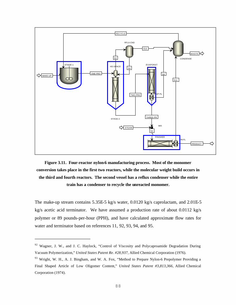
88
MAKE-UP
RECYCLE
ONE-PRO
TWO-PRO
S4
S3
S2
S11
PRODUCT
S8
THREE-PR
S13
WASTE
STEAM
STAGE-1
STAGE-2
HD-SPACEEVAPORAT
FINISHERFIN-FL
EVAP-FL
RFLX-CND
CONDENSE
MIX
Figure 3.11. Four-reactor nylon-6 manufacturing process. Most of the monomer
conversion takes place in the first two reactors, while the molecular weight build occurs in
the third and fourth reactors. The second vessel has a reflux condenser while the entire
train has a condenser to recycle the unreacted monomer.
The make-up stream contains 5.35E-5 kg/s water, 0.0120 kg/s caprolactam, and 2.01E-5
kg/s acetic acid terminator. We have assumed a production rate of about 0.0112 kg/s
polymer or 89 pounds-per-hour (PPH), and have calculated approximate flow rates for
water and terminator based on references 11, 92, 93, 94, and 95.
92 Wagner, J. W., and J. C. Haylock, “Control of Viscosity and Polycaproamide Degradation During
Vacuum Polymerization,” United States Patent Re. #28,937, Allied Chemical Corporation (1976). 93 Wright, W. H., A. J. Bingham, and W. A. Fox, “Method to Prepare Nylon-6 Prepolymer Providing a
Final Shaped Article of Low Oligomer Content,” United States Patent #3,813,366, Allied Chemical
Corporation (1974).
89
The first vessel is a stirred-tank reactor (CSTR), STAGE-1 in Figure 3.11. The residence
time is 8,100 s, the temperature is 488 K, and the pressure is 545,000 Pa.
The second vessel is a plug-flow reactor (STAGE-2 in Figure 3.11). The feed to this
vessel enters a vapor headspace, which we simulate using a flash unit at reactor
conditions (HD-SPACE in Figure 3.11). Vapor from this flash enters the reflux
condenser (RFLX-CND in Figure 3.11). Most of the caprolactam is returned back to the
reactor headspace, while a mixture of caprolactam and water goes to the train condenser
(CONDENSE in Figure 3.11). The reactor has a residence time of 28,800 s, a
temperature of 498 K, and a pressure of 66,700 Pa.
The third reactor is a two-phase plug-flow reactor (PFR, EVAPORAT in Figure 3.11).
The vapor phase is removed via a vacuum system (EVAP-FL in Figure 3.11) and enters
the train condenser CONDENSE. This reactor has a residence time of 1,200 s, a
temperature of 523 K, and a pressure of 2,330 Pa.
The fourth reactor is a two-phase plug-flow reactor (PFR, FINISHER in Figure 3.11).
The vapor phase is removed via a vacuum system (FIN-FL in Figure 3.11) and also enters
the train condenser CONDENSE. We used a sweep-steam mass flow rate of ca. one-
quarter that of the polymer flow rate entering the reactor. This reactor has a residence
time of 7,200 s, a temperature of 536 K, and a pressure of 4,000 Pa.
The train condenser CONDENSE recovers the unreacted monomer and sends it back to
the inlet of the train. Uncondensed species, mostly water, leave in a waste stream. The
condenser operates at an assumed pressure of 101,325 Pa and an assumed temperature of
403 K.
94 Boggs, B. A., L. J. Balint, P. W. Ager, and E. J. Buyalos, “Wiped-Wall Reactor,” United States Patent
#3,976,431, Allied Chemical Corporation (1976). 95 Saunders, L. V. J., and D. Rochell, “Polymer Finisher,” United States Patent #3,686,826, Allied
Chemical Corporation (1972).
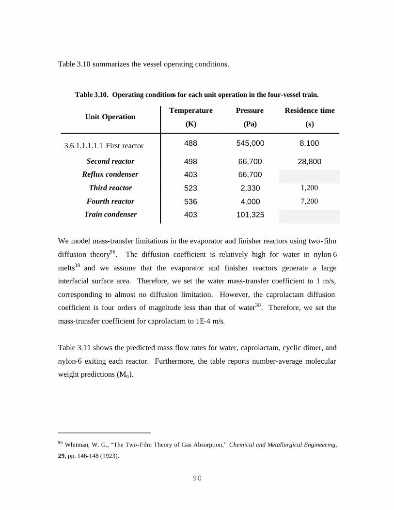
90
Table 3.10 summarizes the vessel operating conditions.
Table 3.10. Operating conditions for each unit operation in the four-vessel train.
Unit Operation Temperature
(K)
Pressure
(Pa)
Residence time
(s)
3.6.1.1.1.1.1 First reactor 488 545,000 8,100
Second reactor 498 66,700 28,800
Reflux condenser 403 66,700
Third reactor 523 2,330 1,200
Fourth reactor 536 4,000 7,200
Train condenser 403 101,325
We model mass-transfer limitations in the evaporator and finisher reactors using two-film
diffusion theory96. The diffusion coefficient is relatively high for water in nylon-6
melts38 and we assume that the evaporator and finisher reactors generate a large
interfacial surface area. Therefore, we set the water mass-transfer coefficient to 1 m/s,
corresponding to almost no diffusion limitation. However, the caprolactam diffusion
coefficient is four orders of magnitude less than that of water38. Therefore, we set the
mass-transfer coefficient for caprolactam to 1E-4 m/s.
Table 3.11 shows the predicted mass flow rates for water, caprolactam, cyclic dimer, and
nylon-6 exiting each reactor. Furthermore, the table reports number-average molecular
weight predictions (Mn).
96 Whitman, W. G., “The Two-Film Theory of Gas Absorption,” Chemical and Metallurgical Engineering,
29, pp. 146-148 (1923).
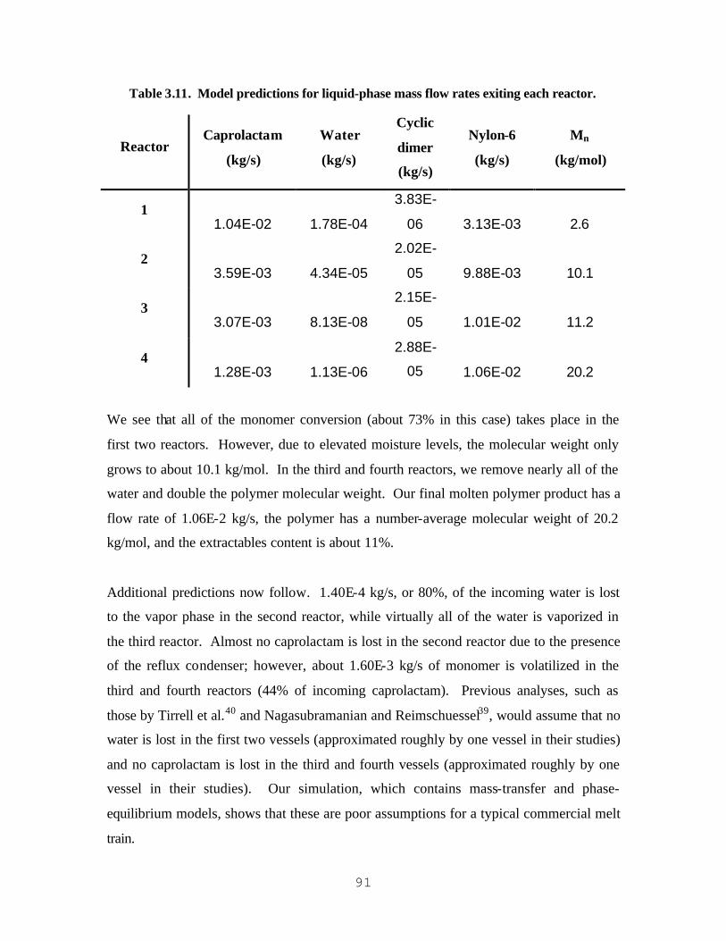
91
Table 3.11. Model predictions for liquid-phase mass flow rates exiting each reactor.
Reactor Caprolactam
(kg/s)
Water
(kg/s)
Cyclic
dimer
(kg/s)
Nylon-6
(kg/s)
Mn
(kg/mol)
1 1.04E-02 1.78E-04
3.83E-
06 3.13E-03 2.6
2 3.59E-03 4.34E-05
2.02E-
05 9.88E-03 10.1
3 3.07E-03 8.13E-08
2.15E-
05 1.01E-02 11.2
4 1.28E-03 1.13E-06
2.88E-
05 1.06E-02 20.2
We see that all of the monomer conversion (about 73% in this case) takes place in the
first two reactors. However, due to elevated moisture levels, the molecular weight only
grows to about 10.1 kg/mol. In the third and fourth reactors, we remove nearly all of the
water and double the polymer molecular weight. Our final molten polymer product has a
flow rate of 1.06E-2 kg/s, the polymer has a number-average molecular weight of 20.2
kg/mol, and the extractables content is about 11%.
Additional predictions now follow. 1.40E-4 kg/s, or 80%, of the incoming water is lost
to the vapor phase in the second reactor, while virtually all of the water is vaporized in
the third reactor. Almost no caprolactam is lost in the second reactor due to the presence
of the reflux condenser; however, about 1.60E-3 kg/s of monomer is volatilized in the
third and fourth reactors (44% of incoming caprolactam). Previous analyses, such as
those by Tirrell et al.40 and Nagasubramanian and Reimschuessel39, would assume that no
water is lost in the first two vessels (approximated roughly by one vessel in their studies)
and no caprolactam is lost in the third and fourth vessels (approximated roughly by one
vessel in their studies). Our simulation, which contains mass-transfer and phase-
equilibrium models, shows that these are poor assumptions for a typical commercial melt
train.
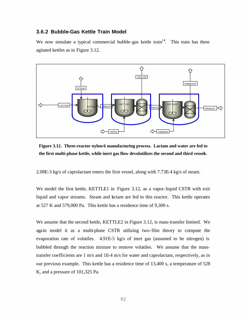
92
3.6.2 Bubble-Gas Kettle Train Model
We now simulate a typical commercial bubble-gas kettle train14. This train has three
agitated kettles as in Figure 3.12.
STEAM
LACTAM ONEOUT
TWON2
TWOVAP
TWOLIQ
THREEN2
THREEVAP
PRODUCTKETTLE1
KETTLE2SEP2
KETTLE3
SEP3
Figure 3.12. Three-reactor nylon-6 manufacturing process. Lactam and water are fed to
the first multi-phase kettle, while inert gas flow devolatilizes the second and third vessels.
2.08E-3 kg/s of caprolactam enters the first vessel, along with 7.73E-4 kg/s of steam.
We model the first kettle, KETTLE1 in Figure 3.12, as a vapor- liquid CSTR with exit
liquid and vapor streams. Steam and lactam are fed to this reactor. This kettle operates
at 527 K and 579,000 Pa. This kettle has a residence time of 9,300 s.
We assume that the second kettle, KETTLE2 in Figure 3.12, is mass-transfer limited. We
again model it as a multi-phase CSTR utilizing two-film theory to compute the
evaporation rate of volatiles. 4.91E-5 kg/s of inert gas (assumed to be nitrogen) is
bubbled through the reaction mixture to remove volatiles. We assume that the mass-
transfer coefficients are 1 m/s and 1E-4 m/s for water and caprolactam, respectively, as in
our previous example. This kettle has a residence time of 13,400 s, a temperature of 528
K, and a pressure of 101,325 Pa.

93
The third kettle, KETTLE3 in Figure 3.12, is identical to the second kettle regarding
operating conditions.
A summary of the vessel operating conditions appears in Table 3.12.
Table 3.12. Operating conditions for each kettle depicted in Figure 3.12. All operating
conditions come from reference 14.
Kettle Temperature
(K) Pressure (Pa)
Residence time
(s)
Steam /
nitrogen flow
rate (kg/s)
1 527 579,000 9,300 7.73E-4
(Steam)
2 528 101,325 13,400 4.91E-5
(Nitrogen)
3 528 101,325 13,400 4.91E-5
(Nitrogen)
Table 3.13 shows the liquid-phase flow rates, compositions, and polymer molecular
weight coming out of each kettle.
Table 3.13. Predicted liquid-stream compositions exiting each kettle.
Kettle Caprolactam
(kg/s)
Water
(kg/s)
Cyclic
dimer
(kg/s)
Nylon-6
(kg/s)
Mn
(kg/mol)
1 4.83E-04 4.77E-05
6.45E-
06 1.51E-03 5.2
2 2.37E-04 3.99E-06
8.71E-
06 1.67E-03 12.4
3 1.89E-04 1.34E-06
9.56E-
06 1.69E-03 20.6

94
With this train, we produce 1.69E-3 kg/s nylon (81% conversion), with 10.5%
extractables coming out of the third kettle. The molecular weight of the polymer is 20.6
kg/mol.
In the first kettle, 75% of the incoming water exits in the vapor stream, along with 4% of
the incoming caprolactam. In the second kettle, the corresponding percentages are 98%
and 18%, respectively. Lastly, the third kettle devolatilizes 80% of the incoming water
and 34% of the incoming caprolactam.
This example again shows that incomplete devolatization based on a more detailed
analysis of the phase equilibrium is more realistic. Using the previous assumptions
regarding nylon phase behavior would have resulted in severe prediction inaccuracies.
3.6.3 Example Summary
These two applications illustrate that we are no longer bound by unrealistic assumptions,
such as no or instantaneous water removal, while ignoring caprolactam devolatization. In
fact, we obtain a high level of detail in our simulations, including an analysis of the
monomer-recovery portion that exists for every realistic manufacturing process. This
high level of modeling detail is possible through the use of our fundamental phase-
equilibrium model for water/caprolactam/nylon-6.
3.7 Conclusions
We have advanced nylon-6 process-simulation technology by developing and
documenting a fundamental phase- equilibrium model. It represents a step forward
towards the generation of a single, consistent model that describes the phase behavior of
all commercially significant nylon polymerization/depolymerization technologies.
In creating this model, we use phase-equilibrium data to characterize the ternary system,
water/caprolactam/nylon-6. We illustrate adequate treatment for inconsistent
thermodynamic data, including the generation of a coherent set of POLYNRTL binary

95
interaction parameters. We then show how to simulate the reactive system,
water/caprolactam/nylon-6, to extract binary interaction parameters for water/nylon-6
segments and caprolactam/nylon-6 segments. Our model predicts the liquid mole
fraction of water with an average error of 1%; previous literature models sometimes
generate predictions that are more than an order of magnitude in error.
After generating a complete model for the phase equilibrium for
water/caprolactam/nylon-6, we validate the interaction parameters by performing
exploratory simulations of commercial manufacturing processes. We simulate a
condenser and match the split fraction for water (99%). We predict a caprolactam split
fraction of 53%, which approximates the real split fraction of 49%.
We also simulate two commercial finishing reactors and show that the models under-
predict the mass fraction of caprolactam in the exit polymer stream. This is in
accordance with expectations: we did not simulate mass-transfer limitations and
therefore, the amount of caprolactam predicted to be in the liquid phase should be low
when compared with plant data.
Lastly, we show two applications of our new phase-equilibrium model in which we
developed integrated process models for entire nylon-6 manufacturing trains. We
simulate wide ranges of temperature and pressure conditions, with temperature ranging
from 403 to 536 K and pressure ranging from 2,330 to 545,000 Pa. We perform
fundamental kinetic, thermodynamic, and mass-transfer calculations to make detailed
predictions about reactor products. These predictions could not be made in the past
without a fundamental phase-equilibrium model.
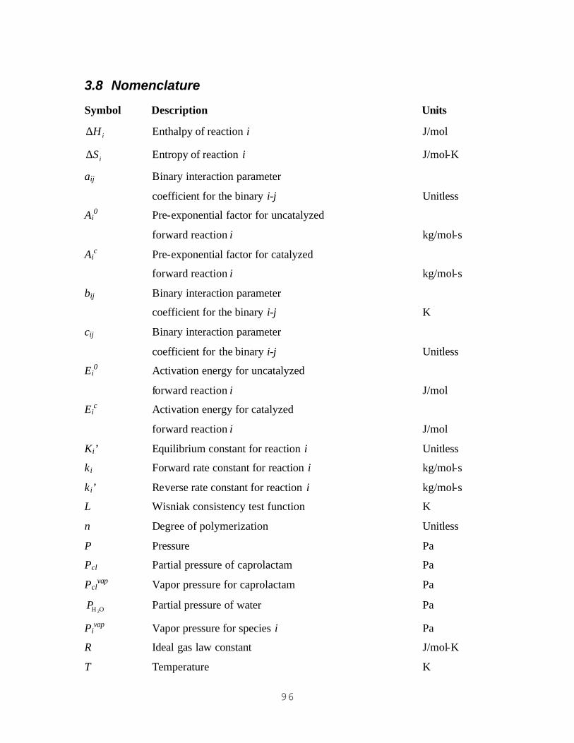
96
3.8 Nomenclature
Symbol Description Units
iH∆ Enthalpy of reaction i J/mol
iS∆ Entropy of reaction i J/mol-K
aij Binary interaction parameter
coefficient for the binary i-j Unitless
Ai0 Pre-exponential factor for uncatalyzed
forward reaction i kg/mol-s
Aic Pre-exponential factor for catalyzed
forward reaction i kg/mol-s
bij Binary interaction parameter
coefficient for the binary i-j K
cij Binary interaction parameter
coefficient for the binary i-j Unitless
Ei0 Activation energy for uncatalyzed
forward reaction i J/mol
Eic Activation energy for catalyzed
forward reaction i J/mol
Ki’ Equilibrium constant for reaction i Unitless
ki Forward rate constant for reaction i kg/mol-s
ki’ Reverse rate constant for reaction i kg/mol-s
L Wisniak consistency test function K
n Degree of polymerization Unitless
P Pressure Pa
Pcl Partial pressure of caprolactam Pa
Pclvap Vapor pressure for caprolactam Pa
2H OP Partial pressure of water Pa
Pivap Vapor pressure for species i Pa
R Ideal gas law constant J/mol-K
T Temperature K

97
iT ° Boiling point for component i K
w Wisniak consistency test function Unitless
W Wisniak consistency test function K
xi Liquid-phase mole fraction of
caprolactam Unitless
xi Liquid-phase mole fraction of
species i Unitless
2H Ox Liquid-phase mole fraction of water Unitless
ycl Vapor-phase mole fraction
of caprolactam Unitless
yi Vapor-phase mole fraction
of species i Unitless
ijα POLYNRTL non-randomness factor
for the binary i-j Unitless
iγ Activity coefficient for species i Unitless
2H Oγ Activity coefficient for water Unitless
is∆ ° Enthalpy of vaporization at the
boiling point for component i J/mol
s∆ Mixture entropy of vaporization J/mol-K
is∆ ° Entropy of vaporization at the boiling
point for component i J/mol-K
ijτ POLYNRTL binary interaction parameter
for the binary i-j Unitless

98
3.9 Supporting Information
Table 3.14. Phase-equilibrium data for the system water/caprolactam at 101,325 Pa
(Manczinger and Tettamanti).
Liquid Mole Fraction
Caprolactam
Vapor Mole Fraction
Caprolactam Temperature (°C)
0.06 0.0003 102
0.08 0.0004 102
0.18 0.0008 106
0.19 0.0010 106
0.23 0.0007 107
0.23 0.0008 107
0.24 0.0008 108
0.30 0.0011 110
0.34 0.0014 112
0.59 0.0033 127
0.62 0.0062 129
0.68 0.0060 135
0.71 0.0135 139
0.77 0.0176 147
0.77 0.0201 147
0.79 0.0193 150
0.84 0.0226 160
Table 3.15. Phase-equilibrium data for the system water/caprolactam at 24,000 Pa
(Manczinger and Tettamanti).
Liquid Mole Fraction
Caprolactam
Vapor Mole Fraction
Caprolactam Temperature (°C)
0.16 0.0002 68
0.18 0.0003 69
0.26 0.0005 71
0.28 0.0006 72
0.40 0.0008 76
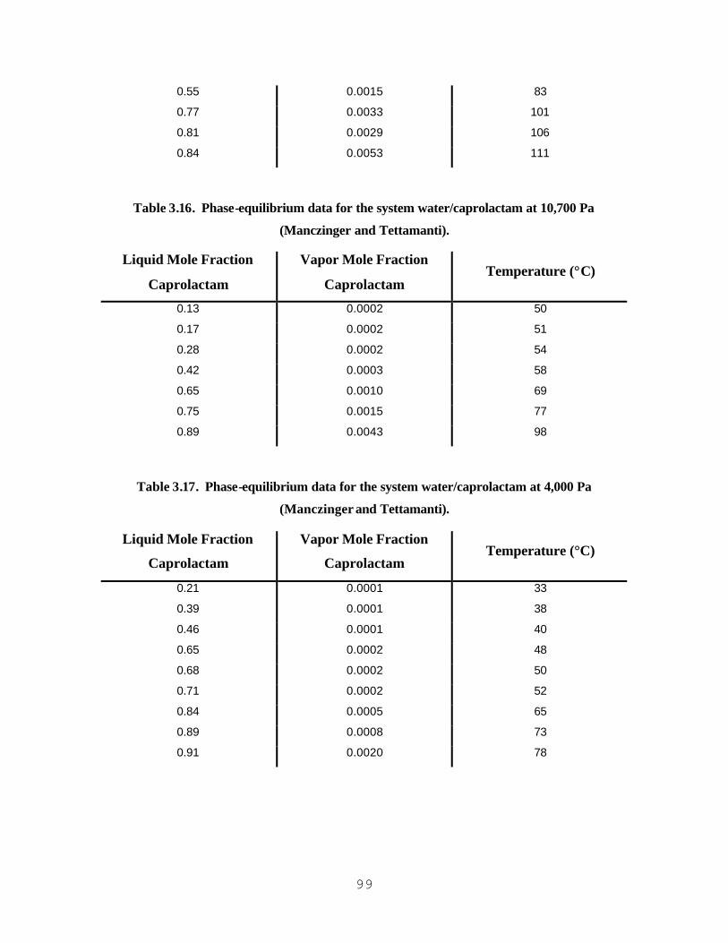
99
0.55 0.0015 83
0.77 0.0033 101
0.81 0.0029 106
0.84 0.0053 111
Table 3.16. Phase-equilibrium data for the system water/caprolactam at 10,700 Pa
(Manczinger and Tettamanti).
Liquid Mole Fraction
Caprolactam
Vapor Mole Fraction
Caprolactam Temperature (°C)
0.13 0.0002 50
0.17 0.0002 51
0.28 0.0002 54
0.42 0.0003 58
0.65 0.0010 69
0.75 0.0015 77
0.89 0.0043 98
Table 3.17. Phase-equilibrium data for the system water/caprolactam at 4,000 Pa
(Manczinger and Tettamanti).
Liquid Mole Fraction
Caprolactam
Vapor Mole Fraction
Caprolactam Temperature (°C)
0.21 0.0001 33
0.39 0.0001 38
0.46 0.0001 40
0.65 0.0002 48
0.68 0.0002 50
0.71 0.0002 52
0.84 0.0005 65
0.89 0.0008 73
0.91 0.0020 78

100
Table 3.18. Phase-equilibrium data for the system water/caprolactam/nylon-6 (Giori and
Hayes). Giori and Hayes used a 0.020-kg caprolactam charge for all polymerizations.
Water charge
(g)
Liquid mole
fraction cl
Liquid mole
fraction water
Vapor mole
fraction water
Equilibrium
pressure (Pa)
0.4 0.10 0.01 0.74 571,473
0.8 0.10 0.02 0.85 1,019,330
1.2 0.10 0.04 0.89 1,399,298
1.6 0.10 0.05 0.89 1,826,890
2.0 0.11 0.07 0.91 2,156,196

101
4 Physical Properties of Nylon-6 Polymerization
Systems
In Chapter 3, we developed a POLYNRTL model for describing the phase equilibrium
inn nylon-6 polymerization mixtures. In this chapter, we add other models to describe
the basic thermophysical properties of the liquid and vapor phases. We are interested in
knowing about phase equilibrium, enthalpies, and molar volumes of these mixtures.
Chapter organization is as follows:
• 4.1 – Tabulation of chemical species that we consider
• 4.2 – Pure-component property models
• 4.3 – Mixture property models
• 4.4 – Phase equilibrium model
• 4.5 – FORTRAN77 implementation of physical property system
• 4.6 – Performance of the simulation
• 4.7 - Conclusions

102
4.1 Introduction to Nylon-6 Polymerization
As we read in Chapter 2, the hydrolytic polymerization of nylon-6 involves seven major
species, including terminators:
1. Initiator - water
2. Monomer – e-caprolactam
3. Byproduct – cyclic dimer
4. Monomer – aminocaproic acid
5. Monofunctional acid terminator – acetic acid
6. Monofunctional amine terminator – cyclohexylamine
7. Polymer – nylon-6 (composed of repeat units and various end groups)
Figure 4.1 shows the molecular structure for all non-polymeric species.
OH2 W
CL
CD
O
OH
CH3
NH2
AA
CHA
NH
O
NH
NH
O
O
Figure 4.1. Non-polymeric species present in nylon-6 polymerization mixtures
Table 4.1 shows the chemical formulas for these non-polymeric species:
Table 4.1. Chemical formulas for non-polymeric species present in nylon-6 polymerization
mixtures
Non-polymeric species Chemical Formula

103
Water H2O
Caprolactam C6H11NO
Cyclic dimer C12H22N2O2
Aminocaproic acid C6H13NO2
Acetic acid C2H4O2
Cyclohexylamine C6H13N
Unlike the simple species, nylon-6 polymer molecules may have a variety of molecular
structures. We describe these molecules as composed of polymer segments. The possible
segments include nylon-6 repeat units (B-ACA), amine end groups (T-NH2), carboxylic
acid end groups (T-COOH), acetic acid end groups (T-HOAC), and cyclohexylamine end
groups (T-CHA); see Figure 4.2.
O
NOHNH
H
NHH
OO
O
CH3
O
NHN
H
B-ACA
T-COOH T-NH2
T-CHA T-HOAC
Figure 4.2. Possible structures of nylon-6: the nylon-6 repeat unit is B-ACA (two covalent
bonds to the rest of the polymer molecule). Possible endgroups are T-COOH or T-CHA
and T-NH2 or T-HOAC (one covalent bond to the rest of the polymer molecule).
All polymer molecules have two end groups – either a carboxyl or cyclohexylamine
endgroup on one end of the chain, and an amine or acetic acid end group on the other end

104
of the chain. Furthermore, the chain can have any number of repeat units. Possible
nylon-6 molecules include:
• T-COOH : T-NH2
• T-COOH : T-HOAC
• T-CHA : T- NH2
• T-CHA : B-ACA : T-HOAC
• T-COOH : (B-ACA)n : T-NH2
The colon represents covalent bonds between segments. The notation (B-ACA)n means a
linear chain of n B-ACA repeat units.
Table 4.2 shows the chemical formulas for each of these polymer segments.
Table 4.2. Chemical formulas for polymer segments
Polymeric segments Chemical Formula
Terminal amine group (T-NH2) C6H12NO
Terminal carboxylic acid group (T-COOH) C6H12NO2
Terminal acetic acid group (T-AA) C2H3O
Terminal cyclohexylamine group (T-CHA) C6H12N
Bound nylon 6 group (B-ACA) C6H11NO
Now we move on to characterizing the physical properties of nylon-6 polymerization
mixtures.
4.2 Pure-Component Physical Properties for Nylon-6
Polymerization
4.2.1 Molecular Weight
We tabulate the molecular weights for all species below (Table 4.3):

105
Table 4.3. Molecular weights for nylon-6 mixtures
Species Molecular weight (g/mol)
Water 18.0152
Caprolactam 113.159
Cyclic dimer 226.318
Aminocaproic acid 131.1742
Acetic acid 60.0524
Cyclohexylamine 99.1754
Nylon-6 (g/mol-seg, B-ACA repeat unit) 113.159
We express the molecular weight of nylon-6 as g/mol-seg. We multiply this number by
the number of segments per molecule (or degree of polymerization) to get the real
polymer molecular weight. We use the number-average degree of polymerization to
calculate the polymer molecular weight.
4.2.2 Critical Constants
We need the critical properties of non-polymeric species to compute the liquid molar
enthalpy. We use the critical temperatures tabulated by the Design Institute for Physical
Property Research (DIPPR)97 (Table 4.4).
Table 4.4. Critical temperature for the species in nylon-6 polymerization mixtures.
Species Tc (K)
Water 6.4713E+02
Caprolactam 8.0600E+02
Cyclic dimer 8.0600E+02
Aminocaproic acid 8.0600E+02
Acetic acid 5.9271E+02
97 Daubert, T. E., and R. P. Danner, Physical and Thermodynamic Properties of Pure Chemicals. Data
Compilation, Volumes 1-3, Hemisphere Publishing Corporation, New York, 1989.

106
Cyclohexylamine 6.1500E+02
For cyclic dimer and aminocaproic acid, we use the critical temperature of caprolactam.
We do so because we do have critical property data for these two molecules. This
approximation does not significantly affect our liquid enthalpy calculations because
cyclic dimer and aminocaproic acid exist in very small quantities relative to nylon-6 and
caprolactam.
4.2.3 Vapor Pressure
We use the DIPPR equation to compute the pure-component vapor pressure siP as a
function of temperature T:
exp ln iEs ii i i i
BP A C T D T
T = + + +
(4.1)
We use the vapor-pressure parameters from Daubert and Danner98 for water,
caprolactam, acetic acid, and cyclohexylamine. Because we do not have vapor pressure
data for cyclic dimer and aminocaproic acid, we assume that these species are non-
volatile.
The assumption that aminocaproic acid is non-volatile does not affect design calculations
for typical hydrolytic polymerizations. This is because it is present in negligible
quantities. However, if one wishes to model a process in which the vaporization of
aminocaproic acid is important, then vapor pressure data should be collected within the
temperature range of interest and vapor pressure parameters regressed.
The assumption that cyclic dimer is non-volatile also does not affect most design
calculations; however, if there is partial devolatization, then model predictions for cyclic
98 Daubert, T. E., and R. P. Danner, Physical and Thermodynamic Properties of Pure Chemicals. Data
Compilation, Volumes 1-3, Hemisphere Publishing Corporation, New York, 1989.
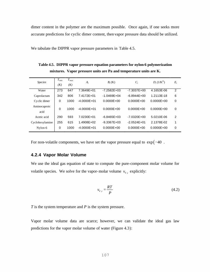
107
dimer content in the polymer are the maximum possible. Once again, if one seeks more
accurate predictions for cyclic dimer content, then vapor pressure data should be utilized.
We tabulate the DIPPR vapor pressure parameters in Table 4.5.
Table 4.5. DIPPR vapor pressure equation parameters for nylon-6 polymerization
mixtures. Vapor pressure units are Pa and temperature units are K.
Species Tmin
(K)
Tmax
(K) Ai Bi (K) Ci Di (1/KE) Ei
Water 273 647 7.3649E+01 -7.2582E+03 -7.3037E+00 4.1653E-06 2
Caprolactam 342 806 7.4172E+01 -1.0469E+04 -6.8944E+00 1.2113E-18 6
Cyclic dimer 0 1000 -4.0000E+01 0.0000E+00 0.0000E+00 0.0000E+00 0
Aminocaproic
acid 0 1000 -4.0000E+01 0.0000E+00 0.0000E+00 0.0000E+00 0
Acetic acid 290 593 7.0230E+01 -6.8465E+03 -7.0320E+00 5.0210E-06 2
Cyclohexylamine 255 615 1.4908E+02 -9.3367E+03 -2.0524E+01 2.1378E-02 1
Nylon-6 0 1000 -4.0000E+01 0.0000E+00 0.0000E+00 0.0000E+00 0
For non-volatile components, we have set the vapor pressure equal to ( )exp 40− .
4.2.4 Vapor Molar Volume
We use the ideal gas equation of state to compute the pure-component molar volume for
volatile species. We solve for the vapor-molar volume ,V iv explicitly:
,V i
RTv
P= (4.2)
T is the system temperature and P is the system pressure.
Vapor molar volume data are scarce; however, we can validate the ideal gas law
predictions for the vapor molar volume of water (Figure 4.3):

108
0
20
40
60
80
100
120
0 50 100 150 200 250 300 350
Temperature (°C)
Wat
er V
apo
r M
ola
r V
olu
me
(m3 /m
ol)
0.05 MPa, Data0.05 MPa, Ideal0.1 MPa, Data0.1 MPa, Ideal0.2 MPa, Data0.2 MPa,Ideal0.3 MPa, Data0.3 MPa, Ideal0.4 MPa, Data0.4 MPa, Ideal
Figure 4.3. Ideal gas vapor molar volume predictions for water (data from Sandler99)
The ideal gas law does not have any problems matching water vapor molar volume data
up to 0.4 MPa and within the temperature range of 100 to 300 °C.
4.2.5 Liquid Molar Volume
We use the DIPPR equation for computing the liquid molar volume of non-polymeric
species:
( )1 1
1Di
i
i
Ti C
i
Av
B
+ −
= (4.3)
99 Sandler, S. I., Chemical and Engineering Thermodynamics, 2nd ed., Wiley, New York, pp. 589-595,
1989.

109
We find DIPPR equation parameters in Daubert and Danner100. We do not find DIPPR
parameters for cyclic dimer and aminocaproic acid. Since these two species exist in such
small quantities in polymerization mixtures and are chemically similar to caprolactam,
we simply approximate their molar volumes as equal to caprolactam (Table 4.6).
Table 4.6. DIPPR liquid molar volume parameters for non-polymeric species (molar
volume in m3/kmol and temperature in K)
Species Tmin (K) Tmzx (K) Ai (kmol/m3) Bi Ci (K) Di
Water 2.7316E+02 3.3315E+02 5.4590E+00 3.0542E-01 6.4713E+02 8.1000E-02
Caprolactam 3.4236E+02 8.0600E+02 7.1180E-01 2.5400E-01 8.0600E+02 2.8570E-01
Cyclic dimer 3.4236E+02 8.0600E+02 7.1180E-01 2.5400E-01 8.0600E+02 2.8570E-01
Aminocaproic
acid 3.4236E+02 8.0600E+02 7.1180E-01 2.5400E-01 8.0600E+02 2.8570E-01
Acetic acid 2.8981E+02 5.9271E+02 1.5791E+00 2.6954E-01 5.9271E+02 2.6843E-01
Cyclohexylamine 2.5545E+02 6.1500E+02 7.0886E-01 2.5517E-01 6.1500E+02 2.7070E-01
We use the Tait equation for the molar volume of polymer. We use data for amorphous
polymer from Zoller101. The equation for the polymer liquid molar volume is below:
( )( )
,,0 1 0.0894ln 1 , 220 °C< T <300 °Ci i
i
P Pav v T
B T
= − +
(4.4)
The equations for the Tait parameters ( ), 0iv T and ( )iB T are below:
( ) ( ) ( )3
2, 0 , 9.4650 04 1.2273 09 ,im
v T E E T Ckg
= − + − ° (4.5)
( ) ( ) ( ) ( ) ( ), 3.3232 08 exp 1 3.8193 03 ,iB T Pa E E T C= + − − ° (4.6)
100 Daubert, T. E., and R. P. Danner, Physical and Thermodynamic Properties of Pure Chemicals. Data
Compilation, Volumes 1-3, Hemisphere Publishing Corporation, New York, 1989. 101 Zoller, P., and D. J. Walsh, Standard Pressure-Volume-Temperature Data for Polymers, Technomic,
Lancaster, p. 278, 1995.
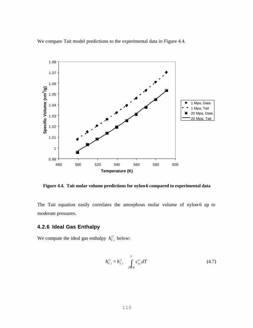
110
We compare Tait model predictions to the experimental data in Figure 4.4.
0.99
1
1.01
1.02
1.03
1.04
1.05
1.06
1.07
1.08
480 500 520 540 560 580 600
Temperature (K)
Sp
ecifi
c V
olu
me
(cm
3 /g)
1 Mpa, Data1 Mpa, Tait20 Mpa, Data20 Mpa, Tait
Figure 4.4. Tait molar volume predictions for nylon-6 compared to experimental data
The Tait equation easily correlates the amorphous molar volume of nylon-6 up to
moderate pressures.
4.2.6 Ideal Gas Enthalpy
We compute the ideal gas enthalpy ,V ih○ below:
, , ,298
T
V i f i p iK
h h c dT= + ∫○ ○ ○ (4.7)

111
,f ih○ is the ideal gas enthalpy of formation at 298 K, ,p ic○ is the ideal gas heat capacity,
and T is the temperature of interest. We use the DIPPR ideal gas heat capacity model.
The integrated form is below:
,298298
coth tanhTT
i ip i i i i i i
KK
C Ec dT AT B C D E
T T= + −∫ ○ (4.8)
We find the ideal gas enthalpy of formation and the parameters for the ideal gas heat
capacity in Daubert and Danner102 (Table 4.7 and Table 4.8). Once again, lacking data
for cyclic dimer and aminocaproic acid, we approximate the ideal gas properties using the
values for caprolactam. This does not impact mixture enthalpy calculations since these
species are present in very small quantities.
Table 4.7. Ideal gas enthalpy of formation
Species Ideal Gas Enthalpy of Formation (J/kmol)
Water -2.4182E+08
Caprolactam -2.4620E+08
Cyclic dimer -2.4620E+08
Aminocaproic acid -2.4620E+08
Acetic acid -4.3225E+08
Cyclohexylamine -1.0490E+08
Table 4.8. DIPPR ideal gas heat capacity parameters (ideal gas heat capacity in J/kmol-K,
temperature in K, upper temperature limit is 1,000 or 1,500 K)
Species Ai (J/kmol-K) Bi (J/kmol-K) Ci (K) Di (J/kmol-K) Ei (K)
Water 3.3359E+04 2.6798E+04 2.6093E+03 8.8880E+03 1.1676E+03
Caprolactam 7.0664E+04 3.7774E+05 -1.5631E+03 2.4215E+05 7.6957E+02
102 Daubert, T. E., and R. P. Danner, Physical and Thermodynamic Properties of Pure Chemicals. Data
Compilation, Volumes 1-3, Hemisphere Publishing Corporation, New York (1989).

112
Cyclic dimer 7.0664E+04 3.7774E+05 -1.5631E+03 2.4215E+05 7.6957E+02
Aminocaproic acid 7.0664E+04 3.7774E+05 -1.5631E+03 2.4215E+05 7.6957E+02
Acetic acid 4.0200E+04 1.3675E+05 1.2620E+03 7.0030E+04 5.6970E+02
Cyclohexylamine 1.9744E+05 2.5599E+05 1.1911E+03 -1.1499E+07 2.3342E+01
4.2.7 Ideal Liquid Enthalpy
We use the following equation to compute the ideal liquid enthalpy ,L ih○ :
, ,s
i
Pv i
L i V i i iPP
vh h h v T dP
T ∂ = − + − ∂
∫○ ○ (4.9)
Since we are using the ideal gas equation of state, the vapor enthalpy departure function
is zero. Therefore, we did not include the vapor enthalpy departure term in Eq. (4.9).
We use the DIPPR equation for the enthalpy of vaporization vih :
( )( )2 3
1 i i r i r i rB C T D T E Tvi i rh A T
+ + += − (4.10)
Tr is the reduced temperature, or T / Tc. Critical temperatures are in Table 4.4. Daubert
and Danner103 tabulate the enthalpy of vaporization parameters for water, caprolactam,
acetic acid, and cyclohexylamine (Table 4.9). We use the caprolactam parameters to
approximate the enthalpy of vaporization for cyclic dimer and aminocaproic acid.
Table 4.9. DIPPR enthalpy of vaporization parameters (enthalpy of vaporization in J/kmol)
Species Tmin (K) Tmax (K) Ai (J/kmol) Bi Ci Di
Water 273 647 5.2053E+07 3.1990E-01 -2.1200E-01 2.5795E-01
Caprolactam 342 806 8.3520E+07 3.7790E-01
103 Daubert, T. E., and R. P. Danner, Physical and Thermodynamic Properties of Pure Chemicals. Data
Compilation, Volumes 1-3, Hemisphere Publishing Corporation, New York, 1989.

113
Cyclic dimer 342 806 8.3520E+07 3.7790E-01
Aminocaproic
acid 342 806 8.3520E+07 3.7790E-01
Acetic acid 290 593 1.2600E+07 -1.1100E+00 6.3000E-02 1.1420E+00
Cyclohexylamine 255 615 5.7160E+07 4.2100E-01
Assuming that the molar volume is not a function of pressure for simple species, we can
use a numerical approximation to the integral in Eq. (4.10):
( ) ( ) ( )
2si
Pi i si
i i iPP P
v T v Tvv T dP v T P P
T
+ ∆ − − ∆ ∂ − = − − ∂ ∆ ∫ (4.11)
2∆ is the temperature interval over which we take our numerical derivative. The
advantage of using a numerical derivative is that one can “swap out” a particular molar
volume model for another one (e.g., changing from DIPPR to Rackett). However, the
disadvantage is a loss of accuracy compared with the analytical solution.
We compute the polymer enthalpy using an equation with the following form:
, , ,ref
ref
T
Lpoly T poly p polyT
h h c= + ∫○ ○ (4.12)
We neglect pressure effects for computing the enthalpy of polymer. This simplification
should not seriously affect our design calculations for two reasons:
• We are most interested in heat of reaction calculations – the enthalpy of the
polymer is fitted to heat of reaction data so that the heat of reaction is predicted
accurately.
• The effect of pressure on the liquid enthalpy is usually negligible – for simple
species like caprolactam, the excess enthalpy accounts for less than 1% of the
total, pure-component liquid enthalpy at pressures above 100 atmospheres.

114
We use the heat capacity expression of Guar et al.104 for amorphous nylon-6:
( ),J
, 0.153 ,K 223.95, 313 K < < 600 Kmol-seg Kppolyc T T= + (4.13)
This expression fits the data very well (Figure 4.5):
265
270
275
280
285
290
295
300
305
310
315
320
300 350 400 450 500 550 600
Temperature (K)
Mo
lten
Nyl
on
-6 H
eat C
apac
ity
(J/m
ol-
seg
K)
DataCorrelation
Figure 4.5. Heat capacity of molten nylon-6
We use enthalpy of polymerization105 to determine the enthalpy of nylon-6 at 313 K. The
enthalpy of reaction is 1.69E+04 J/mol (endothermic reaction). We find a value of the
enthalpy of nylon-6 at 313 K which satisfies the following relation:
104 Guar, U., S. Lau, B. B. Wunderlich, and B. Wunderlich, “Heat Capacity and Other Thermodynamic
Properties of Linear Macro molecules. VIII. Polyesters and Polyamides,” Journal of Physical Chemistry
Reference Data, 12: 65-89, 1983.

115
, ,L poly seg Lcaprolactam rxnh h h− − = ∆○ ○ (4.14)
We regress the enthalpy of nylon-6 at 313 K temperatures ranging from 210 to 240 °C
(Figure 4.6):
-3.30E+05
-3.29E+05
-3.28E+05
-3.27E+05
-3.26E+05
-3.25E+05
-3.24E+05
-3.23E+05
-3.22E+05
-3.21E+05
-3.20E+05483 488 493 498 503 508 513
Temperature (K)
Nyl
on
-6 E
nth
alp
y at
313
K (
J/m
ol-s
eg)
Figure 4.6. Regressed enthalpy of nylon-6 at 313 K
The regressed enthalpy drifts from -3.22E+05 to -3.26E+05 J/mol-seg over a temperature
range of 30 K. This variation is due to the differing enthalpy slopes with temperature
between caprolactam and nylon-6.
105 Arai, Y., K. Tai, H. Teranishi, and T. Tagawa, “Kinetics of Hydrolytic Polymerization of e-Caprolactam: 3.
Formation of Cyclic Dimer,” Polymer, 22: 273-277, 1981.
116
We use an average value of -3.24E+05 J/mol-seg for our calculations. This results in a
9% under-prediction of the enthalpy of reaction at 483 K and a 9% over-prediction of the
enthalpy of reaction at 513 K. Between this range, the error is less.
4.2.8 Polymer Rheology
The rheological properties of nylon-6 vary widely depending on measurement techniques
and molecular-weight distribution. Therefore, we recommend collecting appropriate
experimental data for one’s particular process and polymer grades. We use sample
experimental data to illustrate treatment of rheological data.
We use the non-Newtonian shear viscosity (flow curve) data of Bankar et al106. We show
the flow curves at 230, 250, and 270 °C for a nylon-6 with a number-average molecular
weight of 22,500 g/mol and a molecular-weight polydispersity of 2.08 (Figure 4.7).
106 Bankar, V. G., J. E. Spruiell, and J. L. White, “Melt-Spinning Dynamics and Rheological Properties of
Nylon-6,” Journal of Applied Polymer Science, 21: 2135-2155, 1977.

117
1.00E+02
1.00E+03
1.00E-01 1.00E+00 1.00E+01 1.00E+02 1.00E+03
Shear Rate (1/s)
Sh
ear
Vis
cosi
ty (
Pa
s)
230 °C (Data)250 °C (Data)270 °C (Data)230 °C (CY)250 °C (CY)270 °C (CY)
Figure 4.7. Non-Newtonian shear viscosity of nylon-6 (number-average molecular weight of
22,500 g/mol)
We have fit the curves using the modified Carreau-Yasuda (CY) equation below:
( )( )
01 2 11
1a a
η
ηη γ
τ γ−
= +
&&
(4.15)
0η is the zero-shear viscosity, ητ is a characteristic relaxation time, and a is the breadth-
of-transition parameter. Table 4.10 shows the CY parameters for the three flow curves in
Figure 4.7.

118
Table 4.10. Carreau-Yasuda equation parameters for flow curves of nylon-6 at various
temperatures
Temperature (°C) ( )0 Pa sη ( )sητ a
230 9.9900E+02 3.9698E-03 8.9686E-01
250 5.0232E+02 2.0242E-03 9.0857E-01
270 3.3000E+02 1.2198E-03 9.2506E-01
We designate the flow curve at 230 °C as the reference flow curve. We can approximate
the change of the zero-shear viscosity with weight-average molecular weight using the
following power- law relation:
( )3.4
0 6nylon wA Mη −= (4.16)
For 230 °C, we regress a value of 1.32E-13 Pa s for the constant Anylon-6. We note that at
250 °C, the value is 6.6E-14 Pa s; this compares well with the value of 9.5E-14 Pa s
tabulated in the Polymer Handbook107. We further assume, for purposes of illustration,
that the ratio of the zero-shear viscosity and relaxation time is constant over a range of
molecular weights ( 0ητ η∝ ). This proportionality is suggested by reptation theory108.
Another common form for the relationship between the relaxation time and the zero-shear
viscosity is the form suggested by Bueche’s theory109 of polymer dynamics; this form is a
proportionality of the relaxation time with the product of the zero-shear viscosity and the
weight-average molecular weight ( 0 wMητ η∝ ). The relationship at 230 °C between the
zero-shear viscosity and the relaxation time is below: 107 Mehta, R. H., “Physical Constants of Various Polyamides: Polyamide 6, Polyamide 66, Polyamide 610,
and Polyamide 12,” p. V-127, Polymer Handbook, 4 th ed., J. Brandrup, E. H. Immergut, and E. A. Grulke,
eds., Wiley, New York, 1999. 108 Doi, M., and S. F. Edwards, “Dynamics of Concentrated Polymer Systems. III. The Constitutive
Equation,” J. Chem. Soc. Faraday Trans. II., 74: 1818-1832, 1978. 109 Bueche, F., “Viscosity of Entangled Polymers; Theory of Va riation with Shear Rate,” The Journal of
Chemical Physics, 48: 4781-4784, 1968.

119
( ) ( )0 230 °C230 °C, s 3.97 6 , Pa sEητ η= − (4.17)
We assume that the polydispersity of nylon-6 does not change with molecular weight;
this is approximately true for polymerizations taken to nearly 100% conversion. We
further assume that the Carreau-Yasuda parameter is proportional to some function of the
polydispersity only. This results in a constant a parameter for all nylon-6 polymers at
230 °C with the same polydispersity.
Now that we know how to generate a flow curve at 230 °C for a nylon-6 at any number-
average molecular weight and a polydispersity of two, we turn to predicting the variation
in the flow curve at any temperature above 100 °C plus the glass transition temperature.
We do so using a temperature shift factor aT. We get the shift factor through the
following equation:
0
0 230 °C
TT T
aη
η= (4.18)
The shift factors for the data in Table 4.10 are 0.547 and 0.313 for temperatures 250 °C
and 270 °C, respectively. We correlate the shift factors to temperature using the flow
activation energy H:
1 1
exp230 °CT
Ha
R T = −
(4.19)
We regress a value for the flow activation energy of 66 kJ/mol; this compares well with
the value of 60 kJ/mol found in the Polymer Handbook110.
110 Mehta, R. H., “Physical Constants of Various Polyamides: Polyamide 6, Polyamide 66, Polyamide 610,
and Polyamide 12,” p. V-127, Polymer Handbook, 4 th ed., J. Brandrup, E. H. Immergut, and E. A. Grulke,
eds., Wiley, New York, 1999.

120
We shift the flow curve at 230 °C to any temperature T using the following equations:
230 °C
230 °C
TT T
TT T
a
a
η η
γγ
=
=&& (4.20)
We compute shift factors using equation (4.18) and predict the two higher temperature
flow curves using the flow curve at 230 °C (Figure 4.8):
1.00E+02
1.00E+03
1.00E-01 1.00E+00 1.00E+01 1.00E+02 1.00E+03 1.00E+04
Shear Rate (1/s)
Sh
ear
Vis
cosi
ty (
Pa
s)
230 °C (Data)250 °C (Data)270 °C (Data)230 °C (Shift)250 °C (Shift)270 °C (Shift)
Figure 4.8. Flow curves at 250 and 270 °C predicted using temperature shift factor
We predict the zero-shear viscosity at 250 °C with an error of 9%; we predict the zero-
shear viscosity at 270 °C with an error of -5%.

121
Turning to the intrinsic viscosity of nylon-6, we can estimate it using the Mark-Houwink
constants in the Polymer Handbook111 (Table 4.11). The constants are for a variety of
solvents at 25 °C, and we use the viscosity-average molecular weight:
[ ] a
vK Mη = (4.21)
Table 4.11. Mark-Houwink constants for nylon-6 at 25 °C
Solvent Mv,min (g/mol) Mv,max (g/mol) K (ml/g) a
m-Cresol 0.05E4 0.5E4 320E-3 0.62
Trifluoroethanol 1.3E4 10E4 53.6E-3 0.75
Aq. Formic acid
(85%) 0.7E4 12E4 22.6E-3 0.82
Aq. Formic acid
(65%) 0.7E4 12E4 229E-3 0.5
Aq. Sulfuric
acid 0.3E4 1.3E4 59.2E-3 0.69
We estimate the viscosity-average molecular weight using the number-average molecular
weight112 and by assuming that our sample of nylon-6 follows the most probable
molecular weight distribution:
( ) ( ) 11 1
av nM a a M= + Γ + (4.22)
Lastly, we estimate the formic-acid viscosity of nylon-6 using an expression found in the
literature113:
111 Mehta, R. H., “Physical Constants of Various Polyamides,” in Polymer Handbook (4th ed.) , J. Brandrup,
E. H. Immergut, and E. A. Grulke, eds., Wiley, New York, p. V-127 (1999). 112 Flory, P. J., Principles of Polymer Chemistry, Cornell University Press, Ithaca, New York, p. 313, 1953.
122
( ) ( )2.159.38 9 wFAV E M= − (4.23)
The formic-acid viscosity is a relative viscosity; the ratio of the solution viscosity to the
solvent viscosity (dimensionless). Once again, we show these relationships for
illustrative purposes; re-developing these expressions using in-house measurements is
always recommended for polymer rheology prediction.
4.3 Mixture Properties for Nylon-6 Polymerization
4.3.1 Vapor Molar Volume
We compute the vapor mixture molar volume Vv using the ideal gas equation of state.
Given a temperature T and pressure P, we solve for the vapor molar volume directly
using Eq. (4.2).
4.3.2 Liquid Molar Volume
We use Amagat’s law for approximating the liquid molar volume of a mixture Lv . This
expression uses the mole fraction of each component in the liquid phase xi and the pure-
component liquid molar volume vi:
L i ii
v x v= ∑ (4.24)
4.3.3 Vapor Mixture Enthalpy
We compute the vapor mixture enthalpy using the pure-component, ideal gas enthalpies
and the vapor composition. We use the following model:
113 Akkapeddi, M. K., C. Brown, and B. Vanbuskirk, “Chain Extension of PA-6 and PA-6/66 Copolymer
Via Reactive Extrusion with Triscaprolactamyl Phosphite,” Honeywell Report, http://www.honeywell-
plastics.com/literature/techpapers/0475.pdf, p. 3 (accessed October 2002).

123
,V i V ii
h y h= ∑ ○ (4.25)
iy is the mole fraction of species i in the vapor phase. The ideal gas enthalpy ,V ih○ was
computed in Sec. 13-2.6.
4.3.4 Liquid Mixture Enthalpy
We evaluate the liquid mixture enthalpy Lh using the ideal liquid enthalpy, and then
computing an excess function Eh that estimates departure from ideality:
,E
L i L ii
h x h h= +∑ ○ (4.26)
We use an activity coefficient model to compute the excess function:
2
,
lnE ii
i P x
h RT xTγ∂ = − ∂
∑ (4.27)
We use a finite-difference approximation to evaluate the partial derivative:
ln lnln
2i ii T T
T
γ γγ +∆ − ∆−∂
≈∂ ∆
(4.28)
2∆ is the temperature interval over which we compute our numerical derivative. We
compute the activity coefficient using the POLYNRTL activity coefficient model
(Chapter 3, Sec. 3.2.2.2).
4.4 Vapor-Liquid Equilibrium for Nylon-6 Polymerization
We solve the basic phase-equilibrium equations for each species present in the reaction
mixture:

124
si i i iy P x Pγ= (4.29)
We use the POLYNRTL model to solve for the activity coefficient iγ . We have assumed
that the Poynting correction factors and the fugacity coefficients are one. Our example in
this chapter uses the binary interaction parameters for water-caprolactam binary
interactions (Chapter 3, Sec. 3.4.1).
4.5 FORTRAN 77 Implementation
We implement the principles outlined in the previous sections in a stand-alone
FORTRAN 77 code. We now give that code and provide comments on how it operates.
The code in its entirety appears in Sec. 4.8.
4.5.1 Purpose of the Code
The code takes a specified temperature, pressure, and overall feed (mass flow rate) and
performs a temperature-pressure vapor/liquid flash. It also computes the molar volume
and enthalpy of each phase. These values are stored in the stream vectors that contain all
relevant stream information (Figure 4.9).

125
TemperaturePressure
Mass flow 1Mass flow 2Mass flow 3Mass flow…Mass flow nMole flow 1Mole flow 2Mole flow 3Mole flow…Mole flow n
Degree of Polymerization 1Degree of Polymerization 2Degree of Polymerization 3Degree of Polymerization…Degree of Polymerization n
Molar volumeEnthalpy
Figure 4.9. Stream vector containing stream conditions and flow rates for each species 1
through n. The stream vector also contains the degree of polymerization for each species.
The stream vector has the temperature and pressure of the stream. The stream vector also
contains all flow rates (both mass- and mole-based), degrees of polymerization, and the
molar volume and enthalpy of the streams. The feed stream is called FEED, the liquid
stream is called LIQUID, and the vapor stream is called VAPOR.
The computer program is split into many subroutines that handle very specialized
computations. We split the program into two main parts:
• Computation subroutines – these subroutines perform calculations
• Physical property subroutines – these subroutines store the parameters for the
physical property computations
Table 4.12 contains the names and purposes of the computation subroutines.
Table 4.12. Computation subroutine index
Subroutine name Purpose
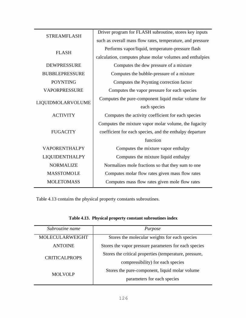
126
STREAMFLASH Driver program for FLASH subroutine, stores key inputs
such as overall mass flow rates, temperature, and pressure
FLASH Performs vapor/liquid, temperature-pressure flash
calculation, computes phase molar volumes and enthalpies
DEWPRESSURE Computes the dew pressure of a mixture
BUBBLEPRESSURE Computes the bubble-pressure of a mixture
POYNTING Computes the Poynting correction factor
VAPORPRESSURE Computes the vapor pressure for each species
LIQUIDMOLARVOLUME Computes the pure-component liquid molar volume for
each species
ACTIVITY Computes the activity coefficient for each species
FUGACITY
Computes the mixture vapor molar volume, the fugacity
coefficient for each species, and the enthalpy departure
function
VAPORENTHALPY Computes the mixture vapor enthalpy
LIQUIDENTHALPY Computes the mixture liquid enthalpy
NORMALIZE Normalizes mole fractions so that they sum to one
MASSTOMOLE Computes molar flow rates given mass flow rates
MOLETOMASS Computes mass flow rates given mole flow rates
Table 4.13 contains the physical property constants subroutines.
Table 4.13. Physical property constant subroutines index
Subroutine name Purpose
MOLECULARWEIGHT Stores the molecular weights for each species
ANTOINE Stores the vapor pressure parameters for each species
CRITICALPROPS Stores the critical properties (temperature, pressure,
compressibility) for each species
MOLVOLP Stores the pure-component, liquid molar volume
parameters for each species
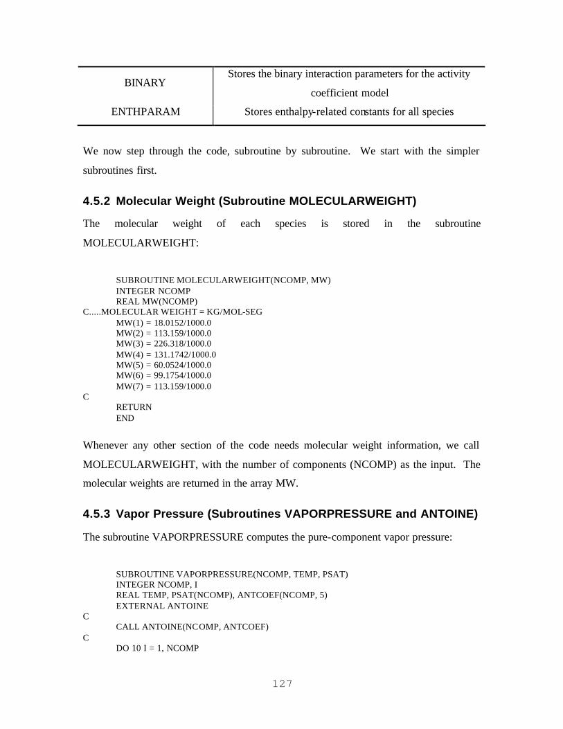
127
BINARY Stores the binary interaction parameters for the activity
coefficient model
ENTHPARAM Stores enthalpy-related constants for all species
We now step through the code, subroutine by subroutine. We start with the simpler
subroutines first.
4.5.2 Molecular Weight (Subroutine MOLECULARWEIGHT)
The molecular weight of each species is stored in the subroutine
MOLECULARWEIGHT:
SUBROUTINE MOLECULARWEIGHT(NCOMP, MW) INTEGER NCOMP REAL MW(NCOMP) C.....MOLECULAR WEIGHT = KG/MOL-SEG MW(1) = 18.0152/1000.0 MW(2) = 113.159/1000.0 MW(3) = 226.318/1000.0 MW(4) = 131.1742/1000.0 MW(5) = 60.0524/1000.0 MW(6) = 99.1754/1000.0 MW(7) = 113.159/1000.0 C RETURN END
Whenever any other section of the code needs molecular weight information, we call
MOLECULARWEIGHT, with the number of components (NCOMP) as the input. The
molecular weights are returned in the array MW.
4.5.3 Vapor Pressure (Subroutines VAPORPRESSURE and ANTOINE)
The subroutine VAPORPRESSURE computes the pure-component vapor pressure:
SUBROUTINE VAPORPRESSURE(NCOMP, TEMP, PSAT) INTEGER NCOMP, I REAL TEMP, PSAT(NCOMP), ANTCOEF(NCOMP, 5) EXTERNAL ANTOINE C CALL ANTOINE(NCOMP, ANTCOEF) C DO 10 I = 1, NCOMP

128
PSAT(I) = EXP(ANTCOEF(I,1)+ANTCOEF(I,2)/TEMP+ANTCOEF(I,3) & *LOG(TEMP)+ANTCOEF(I,4)*TEMP**ANTCOEF(I,5)) 10 CONTINUE C RETURN END The input to the subroutine is the number of components (NCOMP) and the temperature
at which one desires the vapor-pressure calculation (TEMP).
The first line of the executable code calls the ANTOINE subroutine; this subroutine
stores the vapor pressure parameters for all of the species:
SUBROUTINE ANTOINE(NCOMP, ANTCOEF) C.....DAUBERT, T. E., AND R. P. DANNER C.....PHYSICAL AND THERMODYNAMIC PROPERTIES OF PURE CHEMICALS VOLUME 3 INTEGER NCOMP REAL ANTCOEF(NCOMP, 5) C.....VAPOR PRESSURE (PA), TEMPERATURE (K) ANTCOEF(1,1) = 7.3649E+01 ANTCOEF(1,2) = -7.2582E+03 ANTCOEF(1,3) = -7.3037E+00 ANTCOEF(1,4) = 4.1653E-06 ANTCOEF(1,5) = 2.0000E+00 C ANTCOEF(2,1) = 7.4172E+01 ANTCOEF(2,2) = -1.0469E+04 ANTCOEF(2,3) = -6.8944E+00 ANTCOEF(2,4) = 1.2113E-18 ANTCOEF(2,5) = 6.0000E+00 C ANTCOEF(3,1) = -40.0 ANTCOEF(3,2) = 0.0 ANTCOEF(3,3) = 0.0 ANTCOEF(3,4) = 0.0 ANTCOEF(3,5) = 0.0 C ANTCOEF(4,1) = -40.0 ANTCOEF(4,2) = 0.0 ANTCOEF(4,3) = 0.0 ANTCOEF(4,4) = 0.0 ANTCOEF(4,5) = 0.0 C ANTCOEF(5,1) = 7.0230E+01 ANTCOEF(5,2) = -6.8465E+03 ANTCOEF(5,3) = -7.0320E+00 ANTCOEF(5,4) = 5.0210E-06 ANTCOEF(5,5) = 2.0000E+00 C ANTCOEF(6,1) = 1.4908E+02 ANTCOEF(6,2) = -9.3367E+03

129
ANTCOEF(6,3) = -2.0524E+01 ANTCOEF(6,4) = 2.1378E-02 ANTCOEF(6,5) = 1.0000E+00 C ANTCOEF(7,1) = -40.0 ANTCOEF(7,2) = 0.0 ANTCOEF(7,3) = 0.0 ANTCOEF(7,4) = 0.0 ANTCOEF(7,5) = 0.0 C RETURN END
After the subroutine retrieves the vapor pressure parameters (ANTCOEF), it computes
the vapor pressures and returns them in the array PSAT.
4.5.4 Critical Constants (Subroutine CRITICALPROPS)
The subroutine CRITICALPROPS stores the critical property data (temperature,
pressure, compressibility) for each component. The input is the number of components
(NCOMP) and the critical properties are returned in the array CRIT:
SUBROUTINE CRITICALPROPS(NCOMP, CRIT) C.....DAUBERT, T. E., AND R. P. DANNER C.....PHYSICAL AND THERMODYNAMIC PROPERTIES OF PURE CHEMICALS VOLUME 3 INTEGER NCOMP REAL CRIT(NCOMP, 3) C.....CRIT(*,1) = CRITICAL TEMPERATURE (K) C.....CRIT(*,2) = CRITICAL PRESSURE (PA) C.....CRIT(*,3) = CRITICAL COMPRESSIBILITY CRIT(1, 1) = 647.13 CRIT(1, 2) = 2.2055E+07 CRIT(1, 3) = 0.229 C CRIT(2, 1) = 806.0 CRIT(2, 2) = 4.7700E+06 CRIT(2, 3) = 0.286 C CRIT(3, 1) = 806.0 CRIT(3, 2) = 4.7700E+06 CRIT(3, 3) = 0.286 C CRIT(4, 1) = 806.0 CRIT(4, 2) = 4.7700E+06 CRIT(4, 3) = 0.286 C CRIT(5, 1) = 592.71 CRIT(5, 2) = 5.79E+06 CRIT(5, 3) = 0.201 C

130
CRIT(6, 1) = 615.0 CRIT(6, 2) = 4.20E+06 CRIT(6, 3) = 0.296 C CRIT(7, 1) = 647.13 CRIT(7, 2) = 2.2055E+07 CRIT(7, 3) = 0.229 C RETURN END
4.5.5 Vapor Molar Volume, Fugacity Coefficients, and Enthalpy
Departure (Subroutine FUGACITY)
The vapor molar volume, fugacity coefficients, and enthalpy departure function are
computed in the equation of state subroutine, FUGACITY. The subroutine inputs are the
number of components (NCOMP), the temperature (TEMP), the pressure (PRES), and
the vapor composition (Y). It returns the fugacity coefficient for each species
(FUGCOEF), the mixture vapor molar volume (VMOLVOL), and the enthalpy departure
(ENTHALPY):
SUBROUTINE FUGACITY(NCOMP, TEMP, PRES, Y, FUGCOEF, VMOLVOL, & ENTHALPY) INTEGER NCOMP, I, ITMAX, IT REAL TEMP, PRES, Y(NCOMP), FUGCOEF(NCOMP), VMOLVOL, ENTHALPY REAL CRIT(NCOMP, 3), AM, BM, A(NCOMP), B(NCOMP), RIDEAL REAL F, DFDV, TOL PARAMETER (RIDEAL = 8.314, ITMAX = 1000, TOL = 1.0) C VMOLVOL = RIDEAL*TEMP/PRES FUGCOEF = 1.0 ENTHALPY = 0.0 C RETURN END
4.5.6 Binary Interaction Parameters (Subroutine BINARY)
The binary interaction parameters for the POLYNRTL activity coefficient are stored in
the subroutine BINARY. The input is the number of components (NCOMP); the binary
interaction parameters (BININTPAR) are returned:
SUBROUTINE BINARY(NCOMP, BININTPAR)
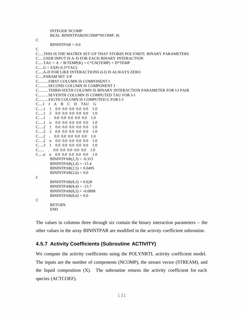
131
INTEGER NCOMP REAL BININTPAR(NCOMP*NCOMP, 8) C BININTPAR = 0.0 C C.....THIS IS THE MATRIX SET-UP THAT STORES POLYNRTL BINARY PARAMETERS C.....USER INPUT IS A-D FOR EACH BINARY INTERACTION C.....TAU = A + B/TEMP(K) + C*LN(TEMP) + D*TEMP C.....G = EXP(-0.3*TAU) C.....A-D FOR LIKE INTERACTIONS (I-I) IS ALWAYS ZERO C.....PARAM SET -UP C..........FIRST COLUMN IS COMPONENT I C..........SECOND COLUMN IS COMPONENT J C..........THIRD-SIXTH COLUMN IS BINARY INTERACTION PARAMETER FOR I-J PAIR C..........SEVENTH COLUMN IS COMPUTED TAU FOR I-J C..........EIGTH COLUMN IS COMPUTED G FOR I-J C.....I J A B C D TAU G C.....1 1 0.0 0.0 0.0 0.0 0.0 1.0 C.....1 2 0.0 0.0 0.0 0.0 0.0 1.0 C.....1 . 0.0 0.0 0.0 0.0 0.0 1.0 C.....1 n 0.0 0.0 0.0 0.0 0.0 1.0 C.....2 1 0.0 0.0 0.0 0.0 0.0 1.0 C.....2 2 0.0 0.0 0.0 0.0 0.0 1.0 C.....2 . 0.0 0.0 0.0 0.0 0.0 1.0 C.....2 n 0.0 0.0 0.0 0.0 0.0 1.0 C.....3 1 0.0 0.0 0.0 0.0 0.0 1.0 C...... . 0.0 0.0 0.0 0.0 0.0 1.0 C.....n n 0.0 0.0 0.0 0.0 0.0 1.0 BININTPAR(2,3) = -0.313 BININTPAR(2,4) = -15.4 BININTPAR(2,5) = 0.0495 BININTPAR(2,6) = 0.0 C BININTPAR(8,3) = 0.628 BININTPAR(8,4) = -13.7 BININTPAR(8,5) = -0.0898 BININTPAR(8,6) = 0.0 C RETURN END
The values in columns three through six contain the binary interaction parameters – the
other values in the array BININTPAR are modified in the activity coefficient subroutine.
4.5.7 Activity Coefficients (Subroutine ACTIVITY)
We compute the activity coefficients using the POLYNRTL activity coefficient model.
The inputs are the number of components (NCOMP), the stream vector (STREAM), and
the liquid composition (X). The subroutine returns the activity coefficient for each
species (ACTCOEF).

132
The first part of the subroutine reads the temperature from the stream vector, reads the
degree of polymerization for each species from the stream vector, and calls the binary
interaction parameter subroutine:
C.....PURPOSE: COMPUTE LIQUID-PHASE ACTIVITY COEFFICIENT USING C...............POLYNRTL ACTIVITY COEFFICIENT MODEL C...............(CHEN, C. C., "A SEGMENT-BASED LOCAL COMPOSITION MODEL FOR THE C................GIBBS ENERGY OF POLYMER SOLUTIONS," FLUID PHASE EQUILIBRIA, C................83, PAGES 301-312 (1993) SUBROUTINE ACTIVITY(NCOMP, STREAM, X, ACTCOEF) INTEGER NCOMP, I REAL STREAM(3*NCOMP+4), X(NCOMP), ACTCOEF(NCOMP), XSEG(NCOMP) REAL BININTPAR(NCOMP*NCOMP, 8), TEMP, DP(NCOMP), XSEGTOT REAL PHIOVERR, FLORY(NCOMP), NRTL(NCOMP) REAL SUM1, SUM2, SUM3, SUM4, SUM5, SUM6 EXTERNAL BINARY C.....READ TEMPERATURE TEMP = STREAM(1) C.....READ DEGREE OF POLYMERIZATION FOR ALL SPECIES DO 10 I = 1, NCOMP DP(I) = STREAM(2+2*NCOMP+I) 10 CONTINUE C.....READ BINARY INTERACTION PARAMETERS CALL BINARY(NCOMP, BININTPAR)
Next, the subroutine computes the POLYNRTL parameters IJτ and GIJ, and computes
the segment-based mole fractions (XSEG):
C.....COMPUTE TAU'S AND G'S DO 20 I = 1, NCOMP**2.0 BININTPAR(I,7) = BININTPAR(I,3) + BININTPAR(I,4)/TEMP + & BININTPAR(I,5)*LOG(TEMP) + BININTPAR(I,6)*TEMP BININTPAR(I,8) = EXP(-0.3*BININTPAR(I,7)) 20 CONTINUE C.....COMPUTE SEGMENT-BASED MOLE FRACTIONS XSEGTOT = 0.0 DO 30 I = 1, NCOMP XSEGTOT = XSEGTOT + X(I)*STREAM(2+2*NCOMP+I) 30 CONTINUE C DO 40 I = 1, NCOMP XSEG(I) = X(I)*STREAM(2+2*NCOMP+I)/XSEGTOT 40 CONTINUE

133
Next, the subroutine computes a portion of the Flory-Huggins contribution to the activity
coefficient, the term k kk
X r∑ :
C.....COMPUTE SUM(PHI(I)/R(I)) PHIOVERR = 0.0 DO 50 I = 1, NCOMP PHIOVERR = PHIOVERR + XSEG(I)/STREAM(2+2*NCOMP+I) 50 CONTINUE C
Lastly, the subroutine computes the activity coefficient for each species. The Flory-
Huggins contribution is first:
DO 80 I = 1, NCOMP C.....COMPUTE FLORY-HUGGINS ACTIVITY COEFFICIENT CONTRIBUTION FLORY(I) = LOG(XSEG(I)/X(I)) + 1.0 - & STREAM(2+2*NCOMP+I)*PHIOVERR
Next, the subroutine computes the local-composition contribution to the activity
coefficient:
C.....COMPUTE NRTL ACTIVITY COEFFICIENT CONTRIBUTION SUM1 = 0.0 SUM5 = 0.0 SUM6 = 0.0 DO 70 J = 1, NCOMP SUM2 = 0.0 SUM3 = 0.0 SUM4 = 0.0 DO 60 K = 1, NCOMP SUM2 = SUM2+XSEG(K)*BININTPAR(NCOMP*(K-1)+J,8) SUM3 = SUM3+XSEG(K)*BININTPAR(NCOMP*(K-1)+J,8)* & BININTPAR(NCOMP*(K-1)+J,7) SUM4 = SUM4+XSEG(K)*BININTPAR(NCOMP*(K-1)+J,8) 60 CONTINUE SUM1 = SUM1 + XSEG(J)*BININTPAR((I-1)*NCOMP+J,8)/SUM2* & (BININTPAR(NCOMP*(I-1)+J,7) - SUM3/SUM4) SUM5 = SUM5 + XSEG(J)*BININTPAR(NCOMP*(J-1)+I,8)* & BININTPAR(NCOMP*(J-1)+I,7) SUM6 = SUM6 + XSEG(J)*BININTPAR(NCOMP*(J-1)+I,8) 70 CONTINUE NRTL(I) = STREAM(2+2*NCOMP+I)*(SUM5/SUM6 + SUM1) C.....COMPUTE ACTUAL ACTIVITY COEFFICIENT ACTCOEF(I) = EXP(FLORY(I) + NRTL(I)) 80 CONTINUE RETURN
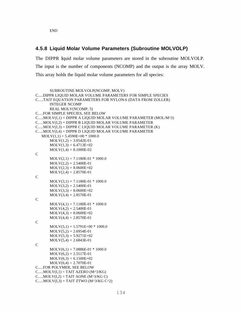
134
END
4.5.8 Liquid Molar Volume Parameters (Subroutine MOLVOLP)
The DIPPR liquid molar volume parameters are stored in the subroutine MOLVOLP.
The input is the number of components (NCOMP) and the output is the array MOLV.
This array holds the liquid molar volume parameters for all species:
SUBROUTINE MOLVOLP(NCOMP, MOLV) C.....DIPPR LIQUID MOLAR VOLUME PARAMETERS FOR SIMPLE SPECIES C.....TAIT EQUATION PARAMETERS FOR NYLON-6 (DATA FROM ZOLLER) INTEGER NCOMP REAL MOLV(NCOMP, 5) C.....FOR SIMPLE SPECIES, SEE BELOW C.....MOLV(I,1) = DIPPR A LIQUID MOLAR VOLUME PARAMETER (MOL/M^3) C.....MOLV(I,2) = DIPPR B LIQUID MOLAR VOLUME PARAMETER C.....MOLV(I,3) = DIPPR C LIQUID MOLAR VOLUME PARAMETER (K) C.....MOLV(I,4) = DIPPR D LIQUID MOLAR VOLUME PARAMETER MOLV(1,1) = 5.4590E+00 * 1000.0 MOLV(1,2) = 3.0542E-01 MOLV(1,3) = 6.4713E+02 MOLV(1,4) = 8.1000E-02 C MOLV(2,1) = 7.1180E-01 * 1000.0 MOLV(2,2) = 2.5400E-01 MOLV(2,3) = 8.0600E+02 MOLV(2,4) = 2.8570E-01 C MOLV(3,1) = 7.1180E-01 * 1000.0 MOLV(3,2) = 2.5400E-01 MOLV(3,3) = 8.0600E+02 MOLV(3,4) = 2.8570E-01 C MOLV(4,1) = 7.1180E-01 * 1000.0 MOLV(4,2) = 2.5400E-01 MOLV(4,3) = 8.0600E+02 MOLV(4,4) = 2.8570E-01 C MOLV(5,1) = 1.5791E+00 * 1000.0 MOLV(5,2) = 2.6954E-01 MOLV(5,3) = 5.9271E+02 MOLV(5,4) = 2.6843E-01 C MOLV(6,1) = 7.0886E-01 * 1000.0 MOLV(6,2) = 2.5517E-01 MOLV(6,3) = 6.1500E+02 MOLV(6,4) = 2.7070E-01 C.....FOR POLYMER, SEE BELOW C.....MOLV(I,1) = TAIT AZERO (M^3/KG) C.....MOLV(I,2) = TAIT AONE (M^3/KG C) C.....MOLV(I,3) = TAIT ZTWO (M^3/KG C^2)

135
C.....MOLV(I,4) = TAIT BZERO (PA) C.....MOLV(I,5) = TAIT BONE (1/C) MOLV(7,1) = 9.4650E-4 MOLV(7,2) = 0.0000E+00 MOLV(7,3) = 1.2273E-09 MOLV(7,4) = 3.3232E+08 MOLV(7,5) = 3.8193E-03 C RETURN END
4.5.9 Pure-Component Liquid Molar Volume (Subroutine
LIQUIDMOLARVOLUME)
The pure-component DIPPR liquid molar volume is computed in the subroutine
LIQUIDMOLARVOLUME. The input to the subroutine is the number of components
(NCOMP) and the stream vector (STREAM). The liquid molar volumes are returned in
the array (LMOLV).
SUBROUTINE LIQUIDMOLARVOLUME(NCOMP, STREAM, LM OLV) INTEGER NCOMP, I REAL LMOLV(NCOMP), MOLV(NCOMP, 5), TEMP, RIDEAL REAL STREAM(3*NCOMP+4), PRES, MW(NCOMP) PARAMETER (RIDEAL = 8.314) EXTERNAL MOLVOLP, MOLECULARWEIGHT C TEMP = STREAM(1) PRES = STREAM(2) C CALL MOLVOLP(NCOMP, MOLV) CALL MOLECULARWEIGHT(NCOMP, MW) C DO 10 I = 1, NCOMP IF(STREAM(2+2*NCOMP+I).EQ.1.0) THEN LMOLV(I) = (MOLV(I,2)**(1.0+(1.0-TEMP/MOLV(I,3)) & **MOLV(I,4)))/MOLV(I,1) ELSE LMOLV(I) = ((MOLV(I,1) + MOLV(I,2)*(TEMP-273.15) + & MOLV(I,3)*(TEMP-273.15)**2.0) * & (1.0 - 0.0894*LOG(1.0 + PRES/(MOLV(I,4)* & EXP(-1.0*MOLV(I,5)*(TEMP-273.15)))))) * & MW(I) * STREAM(2+2*NCOMP+I) END IF 10 CONTINUE C RETURN END

136
The subroutine uses the DIPPR equation for non-polymeric species and the Tait equation
for nylon-6; it identifies the polymer by a non-one degree of polymerization.
4.5.10 Pure-Component Enthalpy Parameters (Subroutine
ENTHPARAM)
The ideal gas enthalpy parameters are stored in the subroutine ENTHPARAM. The input
is the number of components (NCOMP). The output is the ideal gas enthalpy of
formation (IGFORM), the ideal gas DIPPR heat capacity parameters (IGHTCAP), the
DIPPR enthalpy of vaporization parameters (HVAP), and the polymer enthalpy
parameters (HPOLY).
SUBROUTINE ENTHPARAM(NCOMP, IGFORM, IGHTCAP, HVAP, HPOLY) INTEGER NCOMP REAL IGFORM(NCOMP), IGHTCAP(NCOMP,5), HVAP(NCOMP,4), HPOLY(3) C C.....DAUBERT, T. E., AND R. P. DANNER C.....PHYSICAL AND THERMODYNAMIC PROPERTIES OF PURE CHEMICALS VOLUME 3 C C.....VAN KREVELEN, D. W. C.....PROPERTIES OF POLYMERS, 3RD ED., PAGES 112, 123 (1990) C C.....IGFORM = J/KMOL IGFORM(1) = -2.4182E+08 IGFORM(2) = -2.4620E+08 IGFORM(3) = -2.4620E+08 IGFORM(4) = -2.4620E+08 IGFORM(5) = -4.32E+08 IGFORM(6) = -1.05E+08 C.....IGHTCAP = J/KMOL-K IGHTCAP(1, 1) = 3.3359E+04 IGHTCAP(1, 2) = 2.6798E+04 IGHTCAP(1, 3) = 2.6093E+03 IGHTCAP(1, 4) = 8.8880E+03 IGHTCAP(1, 5) = 1.1676E+03 C IGHTCAP(2, 1) = 7.0664E+04 IGHTCAP(2, 2) = 3.7774E+05 IGHTCAP(2, 3) = -1.5631E+03 IGHTCAP(2, 4) = 2.4215E+05 IGHTCAP(2, 5) = 7.6957E+02 C IGHTCAP(3, 1) = 7.0664E+04 IGHTCAP(3, 2) = 3.7774E+05 IGHTCAP(3, 3) = -1.5631E+03 IGHTCAP(3, 4) = 2.4215E+05 IGHTCAP(3, 5) = 7.6957E+02 C

137
IGHTCAP(4, 1) = 7.0664E+04 IGHTCAP(4, 2) = 3.7774E+05 IGHTCAP(4, 3) = -1.5631E+03 IGHTCAP(4, 4) = 2.4215E+05 IGHTCAP(4, 5) = 7.6957E+02 C IGHTCAP(5, 1) = 4.02E+04 IGHTCAP(5, 2) = 1.37E+05 IGHTCAP(5, 3) = 1.26E+03 IGHTCAP(5, 4) = 7.00E+04 IGHTCAP(5, 5) = 5.70E+02 C IGHTCAP(6, 1) = 1.97E+05 IGHTCAP(6, 2) = 2.56E+05 IGHTCAP(6, 3) = 1.19E+03 IGHTCAP(6, 4) = -1.15E+07 IGHTCAP(6, 5) = 2.33E+01 C.....HVAP = J/KMOL HVAP(1, 1) = 5.2053E+07 HVAP(1, 2) = 3.1990E-01 HVAP(1, 3) = -2.1200E-01 HVAP(1, 4) = 2.5795E-01 C HVAP(2, 1) = 8.3520E+07 HVAP(2, 2) = 3.7790E-01 HVAP(2, 3) = 0.0 HVAP(2, 4) = 0.0 C HVAP(3, 1) = 8.3520E+07 HVAP(3, 2) = 3.7790E-01 HVAP(3, 3) = 0.0 HVAP(3, 4) = 0.0 C HVAP(4, 1) = 8.3520E+07 HVAP(4, 2) = 3.7790E-01 HVAP(4, 3) = 0.0 HVAP(4, 4) = 0.0 C HVAP(5, 1) = 1.26E+07 HVAP(5, 2) = -1.11 HVAP(5, 3) = 6.30E-02 HVAP(5, 4) = 1.142 C HVAP(6, 1) = 5.72E+07 HVAP(6, 2) = 0.421 HVAP(6, 3) = 0.0 HVAP(6, 4) = 0.0 C.....HPOLY(1) = REFERENCE ENTHALPY AT 313 K (J/MOL-SEG) C.....HPOLY(2) = CP CONSTANT ONE (J/MOL-SEG K^2) C.....HPOLY(3) = CP CONSTANT TWO (J/MOL-SEG K) HPOLY(1) = -3.24E5 HPOLY(2) = 0.153 HPOLY(3) = 223.95 C RETURN END

138
4.5.11 Mixture Vapor Enthalpy (Subroutine VAPORENTHALPY)
We compute the mixture vapor enthalpy using the subroutine VAPORENTHALPY. The
inputs include the number of components (NCOMP), the stream vector (VAPOR), and
the vapor composition (Y). The mixture vapor enthalpy (VAPENTH) is returned.
The subroutine starts by reading in the temperature, pressure, and enthalpy-model
parameters. Then it computes the vapor pressures:
SUBROUTINE VAPORENTHALPY(NCOMP, VAPOR, Y, VAPENTH) INTEGER NCOMP, I REAL VAPOR(3*NCOMP+4), Y(NCOMP), VAPENTH, TEMP, PRES REAL IGFORM(NCOMP), IGHTCAP(NCOMP, 5), HVAP(NCOMP, 4) REAL HPOLY(3), PSAT(NCOMP), FUGCOEF(NCOMP), VMOLVOL, ENTHALPY REAL EN(NCOMP) EXTERNAL ENTHPARAM, VAPORPRESSURE, FUGACITY C.....READ TEMPERATURE AND PRESSURE TEMP = VAPOR(1) PRES = VAPOR(2) C.....READ ENTHALPY PARAMETERS CALL ENTHPARAM(NCOMP, IGFORM, IGHTCAP, HVAP, HPOLY) C.....COMPUTE VAPOR PRESSURES CALL VAPORPRESSURE(NCOMP, TEMP, PSAT)
Next, the subroutine computes the pure-component ideal gas enthalpies. These are stored
in the array EN:
C.....COMPUTE PURE COMPONENT ENTHALPIES EN = 0.0 DO 10 I = 1, NCOMP IF(VAPOR(2+2*NCOMP+I).EQ.1.0) THEN EN(I) = IGFORM(I) + & (IGHTCAP(I,1)*TEMP + IGHTCAP(I,2)*IGHTCAP(I,3)* & COSH(IGHTCAP(I,3)/TEMP)/SINH(IGHTCAP(I,3)/TEMP) - & IGHTCAP(I,4)*IGHTCAP(I,5)* & SINH(IGHTCAP(I,5)/TEMP)/COSH(IGHTCAP(I,5)/TEMP)) - & (IGHTCAP(I,1)*298.0 + IGHTCAP(I,2)*IGHTCAP(I,3)* & COSH(IGHTCAP(I,3)/298.0)/SINH(IGHTCAP(I,3)/298.0) - & IGHTCAP(I,4)*IGHTCAP(I,5)* & SINH(IGHTCAP(I,5)/298.0)/COSH(IGHTCAP(I,5)/298.0)) EN(I) = EN(I)/1000.0 END IF 10 CONTINUE

139
Next, we use an ideal mixing rule to combine the pure-component enthalpies using the
vapor composition Y:
VAPENTH = 0.0 DO 20 I = 1, NCOMP VAPENTH = VAPENTH + Y(I)*EN(I) 20 CONTINUE
Lastly, we compute the enthalpy departure function using the FUGACITY subroutine:
C.....COMPUTE VAPOR-PHASE ENTHALPY DEPARTURE FROM IDEALITY CALL FUGACITY(NCOMP, TEMP, PRES, Y, FUGCOEF, VMOLVOL, & ENTHALPY) VAPENTH = VAPENTH + ENTHALPY C RETURN END
4.5.12 Mixture Liquid Enthalpy (Subroutine LIQUIDENTHALPY)
We use the subroutine LIQUIDENTHALPY to compute the mixture liquid enthalpy.
The inputs for this subroutine are the number of components (NCOMP), the stream
vector (LIQUID), and the liquid composition (X). The liquid enthalpy is returned in the
variable LIQENTH.
The first part of the subroutine reads the temperature and pressure. It also computes the
vapor pressure and reads in the enthalpy parameters and critical properties:
SUBROUTINE LIQUIDENTHALPY(NCOMP, LIQUID, X, LIQENTH) INTEGER NCOMPM U REAL LIQUID(3*NCOMP+4), LIQENTH, RIDEAL, HINT, X(NCOMP) REAL ACTCOEF(NCOMP), PSAT(NCOMP), TEMP REAL IGFORM(NCOMP), IGHTCAP(NCOMP, 5), HVAP(NCOMP, 4), HPOLY(3) REAL EN(NCOMP), DUMMYX(NCOMP), FUGCOEF(NCOMP), TR REAL ENTHALPY, CRIT(NCOMP, 3), VOL1, VOL2, PRES, ENTHALPYI REAL ACTTEMP2(NCOMP), ACTTEMP1(NCOMP), LMOLV(NCOMP) PARAMETER (RIDEAL = 8.314, HINT = 1.0) EXTERNAL ACTIVITY, VAPORPRESSURE, ENTHPARAM, FUGACITY EXTERNAL CRITICALPROPS C.....READ TEMPERATURE AND PRESSURE TEMP = LIQUID(1) PRES = LIQUID(2) C.....READ ENTHALPY PARAMETERS FOR COMPONENTS
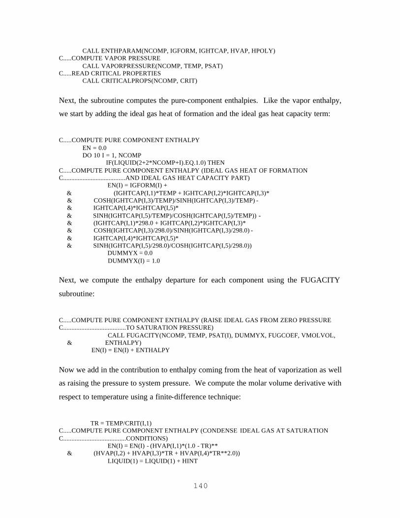
140
CALL ENTHPARAM(NCOMP, IGFORM, IGHTCAP, HVAP, HPOLY) C.....COMPUTE VAPOR PRESSURE CALL VAPORPRESSURE(NCOMP, TEMP, PSAT) C.....READ CRITICAL PROPERTIES CALL CRITICALPROPS(NCOMP, CRIT)
Next, the subroutine computes the pure-component enthalpies. Like the vapor enthalpy,
we start by adding the ideal gas heat of formation and the ideal gas heat capacity term:
C.....COMPUTE PURE COMPONENT ENTHALPY EN = 0.0 DO 10 I = 1, NCOMP IF(LIQUID(2+2*NCOMP+I).EQ.1.0) THEN C.....COMPUTE PURE COMPONENT ENTHALPY (IDEAL GAS HEAT OF FORMATION C......................................AND IDEAL GAS HEAT CAPACITY PART) EN(I) = IGFORM(I) + & (IGHTCAP(I,1)*TEMP + IGHTCAP(I,2)*IGHTCAP(I,3)* & COSH(IGHTCAP(I,3)/TEMP)/SINH(IGHTCAP(I,3)/TEMP) - & IGHTCAP(I,4)*IGHTCAP(I,5)* & SINH(IGHTCAP(I,5)/TEMP)/COSH(IGHTCAP(I,5)/TEMP)) - & (IGHTCAP(I,1)*298.0 + IGHTCAP(I,2)*IGHTCAP(I,3)* & COSH(IGHTCAP(I,3)/298.0)/SINH(IGHTCAP(I,3)/298.0) - & IGHTCAP(I,4)*IGHTCAP(I,5)* & SINH(IGHTCAP(I,5)/298.0)/COSH(IGHTCAP(I,5)/298.0)) DUMMYX = 0.0 DUMMYX(I) = 1.0
Next, we compute the enthalpy departure for each component using the FUGACITY
subroutine:
C.....COMPUTE PURE COMPONENT ENTHALPY (RAISE IDEAL GAS FROM ZERO PRESSURE C......................................TO SATURATION PRESSURE) CALL FUGACITY(NCOMP, TEMP, PSAT(I), DUMMYX, FUGCOEF, VMOLVOL, & ENTHALPY) EN(I) = EN(I) + ENTHALPY
Now we add in the contribution to enthalpy coming from the heat of vaporization as well
as raising the pressure to system pressure. We compute the molar volume derivative with
respect to temperature using a finite-difference technique:
TR = TEMP/CRIT(I,1) C.....COMPUTE PURE COMPONENT ENTHALPY (CONDENSE IDEAL GAS AT SATURATION C......................................CONDITIONS) EN(I) = EN(I) - (HVAP(I,1)*(1.0 - TR)** & (HVAP(I,2) + HVAP(I,3)*TR + HVAP(I,4)*TR**2.0)) LIQUID(1) = LIQUID(1) + HINT

141
CALL LIQUIDMOLARVOLUME(NCOMP, LIQUID, LMOLV) LIQUID(1) = LIQUID(1) - HINT VOL2 = LMOLV(I) LIQUID(1) = LIQUID(1) - HINT CALL LIQUIDMOLARVOLUME(NCOMP, LIQUID, LMOLV) LIQUID(1) = LIQUID(1) + HINT VOL1 = LMOLV(I) CALL LIQUIDMOLARVOLUME(NCOMP, LIQUID, LMOLV) C.....COMPUTE PURE COMPONENT ENTHALPY (BRING LIQUID TO SYSTEM PRESSURE) EN(I) = EN(I) + (LMOLV(I) - TEMP* & ((VOL2 - VOL1)/(2.0*HINT)))*(PRES - PSAT(I)) C.....CONVERT J/KMOL TO J/MOL EN(I) = EN(I) / 1000.0
For polymer, we use a simpler equation to compute the pure-component liquid enthalpy;
we use the enthalpy at 313 K and a liquid heat capacity model to raise our system to
system temperature. We ignore pressure effects.
ELSE C.....PURE COMPONENT LIQUID ENTHALPY FOR POLYMER EN(I) = LIQUID(2+2*NCOMP+I)* & (HPOLY(1) + (HPOLY(2)/2.0*TEMP**2.0 + HPOLY(3)*TEMP) & - (HPOLY(2)/2.0*313.0**2.0 + HPOLY(3)*313.0)) END IF 10 CONTINUE
Next, we use a mixing rule to arrive at the ideal liquid enthalpy:
C.....COMPUTE MIXTURE ENTHALPY WITHOUT EXCESS ENTHALPY OF MIXING EFFECTS ENTHALPYI = 0.0 DO 20 I = 1, NCOMP ENTHALPYI = ENTHALPYI + X(I)*EN(I) 20 CONTINUE
The excess enthalpy function for the liquid phase is computed using a finite difference
technique; the activity coefficients are furnished by the ACTIVITY subroutine. Lastly,
the excess enthalpy is added to the ideal liquid enthalpy:
LIQUID(1) = LIQUID(1) + HINT CALL ACTIVITY(NCOMP, LIQUID, X, ACTCOEF) LIQUID(1) = LIQUID(1) - HINT ACTTEMP2 = ACTCOEF LIQUID(1) = LIQUID(1) - HINT CALL ACTIVITY(NCOMP, LIQUID, X, ACTCOEF) LIQUID(1) = LIQUID(1) + HINT ACTTEMP1 = ACTCOEF

142
C LIQENTH = 0.0 DO 30 I = 1, NCOMP LIQENTH = LIQENTH + (LOG(ACTTEMP2(I))-LOG(ACTTEMP1(I)))/ & (2.0*HINT)*X(I) 30 CONTINUE C.....COMPUTE EXCESS ENTHALPY OF MIXING LIQENTH = LIQENTH*(-1.0)*(TEMP**2.0)*RIDEAL C LIQENTH = LIQENTH + ENTHALPYI C RETURN END
4.5.13 Poynting Correction (Subroutine POYNTING)
The subroutine POYNTING computes the Poynting correction factor for all species. The
inputs include the number of components (NCOMP), the liquid molar volumes
(LMOLV), the temperature (TEMP), the pressure (PRES), and the vapor pressures
(PSAT). The Poynting correction factor is return in the array POYNT.
SUBROUTINE POYNTING(NCOMP, LMOLV, TEMP, PRES, PSAT, POYNT) INTEGER NCOMP, I REAL LMOLV(NCOMP), PRES, PSAT(NCOMP), POYNT(NCOMP), TEMP REAL RIDEAL PARAMETER (RIDEAL = 8.314) C POYNT = 1.0 C RETURN END
4.5.14 Normalization of Composition Variables (Subroutine
NORMALIZE)
We use the NORMALIZE subroutine to normalize mole fractions so that they sum to
one. We require this operation in the VLE calculations. This subroutine requires the
mole fraction array X and the number of components (NCOMP). The normalized mole
fractions are returned in the array X.
C.....PURPOSE: THIS SUBROUTINE NORMALIZES MOLE FRACTIONS SUBROUTINE NORMALIZE(NCOMP, X) INTEGER NCOMP, I

143
REAL X(NCOMP), TOT C TOT = 0.0 DO 10 I = 1, NCOMP TOT = TOT + X(I) 10 CONTINUE C DO 20 I = 1, NCOMP X(I) = X(I)/TOT 20 CONTINUE C RETURN END
4.5.15 Mole-to-Mass and Mass-to-Mole Conversions
(Subroutines MOLETOMASS and MASSTOMOLE)
Two subroutines convert molar flow rates to mass flow rates (MOLETOMASS) and vice
versa (MASSTOMOLE). These subroutines use mole/mass information and use it to fill
in empty spaces of the stream vector.
SUBROUTINE MASSTOMOLE(NCOMP, STREAM) INTEGER NCOMP, I REAL STREAM(3*NCOMP+4), MW(NCOMP) EXTERNAL MOLECULARWEIGHT C CALL MOLECULARWEIGHT(NCOMP, MW) C DO 10 I = 1, NCOMP STREAM(NCOMP+2+I) = STREAM(2+I)/(MW(I)*STREAM(2*NCOMP+2+I)) 10 CONTINUE C RETURN END
SUBROUTINE MOLETOMASS(NCOMP, STREAM) INTEGER NCOMP, I REAL STREAM(3*NCOMP+4), MW(NCOMP) EXTERNAL MOLECULARWEIGHT C CALL MOLECULARWEIGHT(NCOMP, MW) C DO 10 I = 1, NCOMP STREAM(2+I) = STREAM(NCOMP+2+I)*MW(I)*STREAM(2*NCOMP+2+I) 10 CONTINUE C RETURN END

144
4.5.16 Dew Pressure Computation (Subroutine DEWPRESSURE)
The subroutine DEWPRESSURE computes the dew pressure of a mixture. As inputs, the
subroutine takes the number of components (NCOMP) and the stream vector (STREAM).
It returns the dew pressure (DEWP) and the activity/fugacity coefficients at the dew point
(ACTDEW and FUGDEW, respectively).
The first part of the subroutine computes the overall composition variable Z, and sets it
equal to the vapor composition Y:
SUBROUTINE DEWPRESSURE(NCOMP, STREAM, DEWP, ACTDEW, FUGDEW) INTEGER NCOMP, I REAL STREAM(3*NCOMP+4), ACTDEW(NCOMP), FUGDEW(NCOMP), DEWP REAL PSAT(NCOMP), LMOLV(NCOMP), Y(NCOMP), TEMP, STOT REAL X(NCOMP), VMOLVOL, ENTHALPY, POYNT(NCOMP), ACTOLD(NCOMP) REAL ERROR1, ERROR2, DEWPOLD, TOL1, TOL2 PARAMETER (TOL1 = 10.0, TOL2 = 1.0E-5) EXTERNAL VAPORPRESSURE, LIQUIDMOLARVOLUME, ACTIVITY, NORMALIZE EXTERNAL FUGACITY, POYNTING C.....READ TEMPERATURE TEMP = STREAM(1) C.....SET Y = Z STOT = 0.0 DO 10 I = 1, NCOMP STOT = STOT + STREAM(2+NCOMP+I) 10 CONTINUE C DO 20 I = 1, NCOMP Y(I) = STREAM(2+NCOMP+I)/STOT 20 CONTINUE
Next, we set fugacity and activity coefficients to one and compute the vapor pressure and
liquid molar volumes. We also estimate the dew pressure and liquid composition and
then refine the dew pressure estimate using non- ideal activity coefficients:
C.....SET ACTIVITY/FUGACITY COEFFICIENTS EQUAL TO ONE FUGDEW = 1.0 ACTDEW = 1.0 C.....COMPUTE VAPOR PRESSURE CALL VAPORPRESSURE(NCOMP, TEMP, PSAT) C.....COMPUTE LIQUID MOLAR VOLUMES CALL LIQUIDMOLARVOLUME(NCOMP, STREAM, LMOLV) C.....COMPUTE DEW PRESSURE DEWP = 0.0 DO 30 I = 1, NCOMP DEWP = DEW P + Y(I)*FUGDEW(I)/ACTDEW(I)/PSAT(I)

145
30 CONTINUE DEWP = 1.0/DEWP C.....COMPUTE X DO 40 I = 1, NCOMP X(I) = Y(I)*DEWP/PSAT(I) 40 CONTINUE C.....NORMALIZE X CALL NORMALIZE(NCOMP, X) C.....COMPUTE ACTIVITY COEFFICIENT CALL ACTIVITY(NCOMP, STREAM, X, ACTDEW) C.....COMPUTE DEW PRESSURE DEWP = 0.0 DO 50 I = 1, NCOMP DEWP = DEWP + Y(I)*FUGDEW(I)/PSAT(I)/ACTDEW(I) 50 CONTINUE DEWP = 1.0/DEWP
Next, we enter the dew pressure convergence loop (outer loop). We start this loop by
computing non- ideal fugacity coefficients and the Poynting correction factor.
C.....COMPUTE FUGACITY COEFFICIENT 60 CALL FUGACITY(NCOMP, TEMP, DEWP, Y, FUGDEW, VMOLVOL, ENTHALPY) C.....COMPUTE POYNTING CORRECTION FACTOR CALL POYNTING(NCOMP, LMOLV, TEMP, DEWP, PSAT, POYNT)
We now enter the activity coefficient convergence loop (inner loop).
C.....COMPUTE X 70 DO 80 I = 1, NCOMP X(I) = Y(I)*FUGDEW(I)*DEWP/ACTDEW(I)/PSAT(I)/POYNT(I) 80 CONTINUE C.....NORMALIZE X CALL NORMALIZE(NCOMP, X) C.....COMPUTE ACTIVITY COEFFICIENTS ACTOLD = ACTDEW CALL ACTIVITY(NCOMP, STREAM, X, ACTDEW) C.....COMPUTE CHANGE IN ACTIVITY COEFFICIENTS SINCE LAST ITERATION ERROR1 = 0.0 DO 90 I = 1, NCOMP ERROR1 = ERROR1 + (ACTDEW(I)-ACTOLD(I))**2.0 90 CONTINUE
Here we check the relative change in the activity coefficients. If it is below the specified
tolerance, then we exit the inner loop.
C.....CHECK TOLERANCE (ACTIVITY COEFFICIENT CONVERGENCE LOOP) IF(ERROR1.GT.TOL1) THEN GO TO 70

146
END IF C DEWPOLD = DEWP C.....COMPUTE DEW PRESSURE DEWP = 0.0 DO 100 I = 1, NCOMP DEWP = DEWP + Y(I)*FUGDEW(I)/ACTDEW(I)/PSAT(I)/POYNT(I) 100 CONTINUE DEWP = 1.0/DEWP C.....COMPUTE CHANGE IN DEW PRESSURE ERROR2 = (DEWP - DEWPOLD)**2.0
We now check the relative change in the estimated dew pressure. If it is below the
specified tolerance, we exit the outer convergence loop.
C.....CHECK TOLERANCE (DEW PRESSURE CONVERGENCE LOOP) IF(ERROR2.GT.TOL2) THEN GO TO 60 END IF C RETURN END
4.5.17 Bubble Pressure Computation (Subroutine
BUBBLEPRESSURE)
The BUBBLEPRESSURE subroutine computes the bubble pressure for a mixture. The
input for this subroutine includes the number of components (NCOMP) and the stream
vector (STREAM). The subroutine returns the bubble pressure (BUBP) and the
activity/fugacity coefficients at the bubble point (ACTBUB and FUGBUB, respectively).
The first part of the subroutine reads the temperature, computes the overall composition
variable Z, and sets the liquid composition X to the overall composition.
SUBROUTINE BUBBLEPRESSURE(NCOMP, STREAM, BUBP, ACTBUB, FUGBUB) INTEGER NCOMP, I REAL STREAM(3*NCOMP+4), BUBP, ACTBUB(NCOMP), FUGBUB(NCOMP) REAL PSAT(NCOMP), TEMP, LMOLV(NCOMP), POYNT(NCOMP), STOT REAL X(NCOMP), Y(NCOMP), VMOLVOL, ENTHALPY, BUBPOLD, ERROR, TOL PARAMETER (TOL = 1.0E-05) EXTERNAL POYNTING, VAPORPRESSURE, FUGACITY, ACTIVITY, NORMALIZE C.....READ TEMPERATURE TEMP = STREAM(1) C.....SET X = Z

147
STOT = 0.0 DO 10 I = 1, NCOMP STOT = STOT + STREAM(2+NCOMP+I) 10 CONTINUE C DO 20 I = 1, NCOMP X(I) = STREA M(2+NCOMP+I)/STOT 20 CONTINUE
We now set the fugacity coefficient equal to one and compute the vapor pressures and
liquid molar volumes. We also compute the activity coefficients and estimate the bubble
pressure:
C.....SET FUGACITY COEFFICIENTS EQUAL TO ONE FUGBUB = 1.0 C.....COMPUTE VAPOR PRESSURE CALL VAPORPRESSURE(NCOMP, TEMP, PSAT) C.....COMPUTE LIQUID MOLAR VOLUME CALL LIQUIDMOLARVOLUME(NCOMP, STREAM, LMOLV) C.....COMPUTE ACTIVITY COEFFICIENTS CALL ACTIVITY(NCOMP, STREAM, X, ACTBUB) C.....COMPUTE BUBBLE PRESSURE BUBP = 0.0 DO 30 I = 1, NCOMP BUBP = BUBP + X(I)*ACTBUB(I)*PSAT(I)/FUGBUB(I) 30 CONTINUE
Here we enter the bubble pressure convergence loop. We continuously refine our
estimates of the vapor composition at the bubble point, the fugacity coefficients at the
bubble point, and the bubble pressure:
C.....COMPUTE POYNTING CORRECTION FACTORS 40 CALL POYNTING(NCOMP, LMOLV, TEMP, BUBP, PSAT, POYNT) C.....COMPUTE Y DO 50 I = 1, NCOMP Y(I) = X(I)*ACTBUB(I)*PSAT(I)*POYNT(I)/FUGBUB(I)/BUBP 50 CONTINUE C.....NORMALIZE Y CALL NORMALIZE(NCOMP, Y) C.....COMPUTE FUGACITY COEFFICIENTS CALL FUGACITY(NCOMP, TEMP, BUBP, Y, FUGBUB, VMOLVOL, ENTHALPY) C BUBPOLD = BUBP C.....COMPUTE BUBBLE PRESSURE BUBP = 0.0 DO 60 I = 1, NCOMP BUBP = BUBP + X(I)*ACTBUB(I)*PSAT(I)*POYNT(I)/FUGBUB(I) 60 CONTINUE
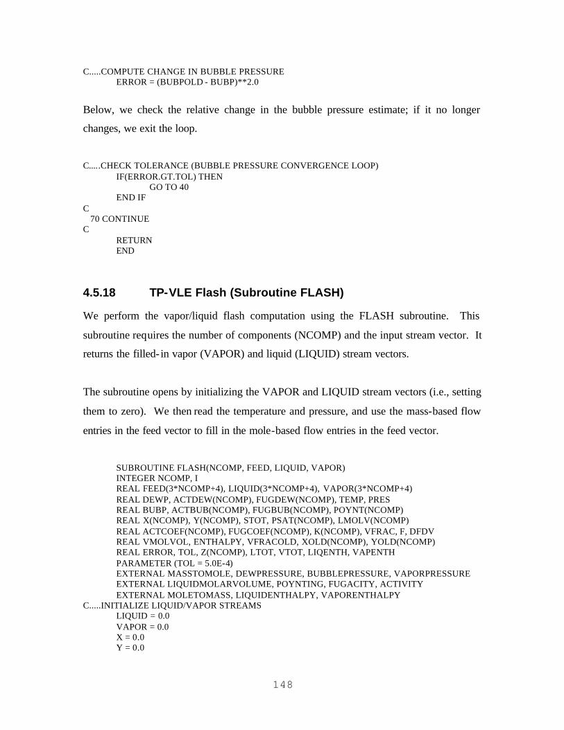
148
C.....COMPUTE CHANGE IN BUBBLE PRESSURE ERROR = (BUBPOLD - BUBP)**2.0
Below, we check the relative change in the bubble pressure estimate; if it no longer
changes, we exit the loop.
C.....CHECK TOLERANCE (BUBBLE PRESSURE CONVERGENCE LOOP) IF(ERROR.GT.TOL) THEN GO TO 40 END IF C 70 CONTINUE C RETURN END
4.5.18 TP-VLE Flash (Subroutine FLASH)
We perform the vapor/liquid flash computation using the FLASH subroutine. This
subroutine requires the number of components (NCOMP) and the input stream vector. It
returns the filled- in vapor (VAPOR) and liquid (LIQUID) stream vectors.
The subroutine opens by initializing the VAPOR and LIQUID stream vectors (i.e., setting
them to zero). We then read the temperature and pressure, and use the mass-based flow
entries in the feed vector to fill in the mole-based flow entries in the feed vector.
SUBROUTINE FLASH(NCOMP, FEED, LIQUID, VAPOR) INTEGER NCOMP, I REAL FEED(3*NCOMP+4), LIQUID(3*NCOMP+4), VAPOR(3*NCOMP+4) REAL DEWP, ACTDEW(NCOMP), FUGDEW(NCOMP), TEMP, PRES REAL BUBP, ACTBUB(NCOMP), FUGBUB(NCOMP), POYNT(NCOMP) REAL X(NCOMP), Y(NCOMP), STOT, PSAT(NCOMP), LMOLV(NCOMP) REAL ACTCOEF(NCOMP), FUGCOEF(NCOMP), K(NCOMP), VFRAC, F, DFDV REAL VMOLVOL, ENTHALPY, VFRACOLD, XOLD(NCOMP), YOLD(NCOMP) REAL ERROR, TOL, Z(NCOMP), LTOT, VTOT, LIQENTH, VAPENTH PARAMETER (TOL = 5.0E-4) EXTERNAL MASSTOMOLE, DEWPRESSURE, BUBBLEPRESSURE, VAPORPRESSURE EXTERNAL LIQUIDMOLARVOLUME, POYNTING, FUGACITY, ACTIVITY EXTERNAL MOLETOMASS, LIQUIDENTHALPY, VAPORENTHALPY C.....INITIALIZE LIQUID/VAPOR STREAMS LIQUID = 0.0 VAPOR = 0.0 X = 0.0 Y = 0.0
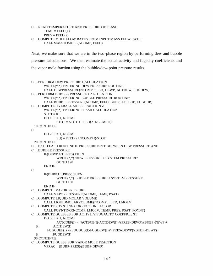
149
C.....READ TEMPERATURE AND PRESSURE OF FLASH TEMP = FEED(1) PRES = FEED(2) C.....COMPUTE MOLE FLOW RATES FROM INPUT MASS FLOW RATES CALL MASSTOMOLE(NCOMP, FEED)
Next, we make sure that we are in the two-phase region by performing dew and bubble
pressure calculations. We then estimate the actual activity and fugacity coefficients and
the vapor mole fraction using the bubble/dew-point pressure results.
C.....PERFORM DEW PRESSURE CALCULATION WRITE(*,*) 'ENTERING DEW PRESSURE ROUTINE' CALL DEWPRESSURE(NCOMP, FEED, DEWP, ACTDEW, FUGDEW) C.....PERFORM BUBBLE PRESSURE CALCULATION WRITE(*,*) 'ENTERING BUBBLE PRESSURE ROUTINE' CALL BUBBLEPRESSURE(NCOMP, FEED, BUBP, ACTBUB, FUGBUB) C.....COMPUTE OVERALL MOLE FRACTION Z WRITE(*,*) 'ENTERING FLASH CALCULATION' STOT = 0.0 DO 10 I = 1, NCOMP STOT = STOT + FEED(2+NCOMP+I) 10 CONTINUE C DO 20 I = 1, NCOMP Z(I) = FEED(2+NCOMP+I)/STOT 20 CONTINUE C.....EXIT FLASH ROUTINE IF PRESSURE ISN'T BETWEEN DEW PRESSURE AND C.....BUBBLE PRESSURE IF(DEWP.GT.PRES) THEN WRITE(*,*) 'DEW PRESSURE > SYSTEM PRESSURE' GO TO 120 END IF C IF(BUBP.LT.PRES) THEN WRITE(*,*) 'BUBBLE PRESSURE < SYSTEM PRESSURE' GO TO 130 END IF C.....COMPUTE VAPOR PRESSURE CALL VAPORPRESSURE(NCOMP, TEMP, PSAT) C.....COMPUTE LIQUID MOLAR VOLUME CALL LIQUIDMOLARVOLUME(NCOMP, FEED, LMOLV) C.....COMPUTE POYNTING CORRECTION FACTOR CALL POYNTING(NCOMP, LMOLV, TEMP, PRES, PSAT, POYNT) C.....COMPUTE GUESSES FOR ACTIVITY/FUGACITY COEFFICIENT DO 30 I = 1, NCOMP ACTCOEF(I) = (ACTBUB(I)-ACTDEW(I))*(PRES -DEWP)/(BUBP-DEWP)+ & ACTDEW(I) FUGCOEF(I) = (FUGBUB(I)-FUGDEW(I))*(PRES-DEWP)/ (BUBP-DEWP)+ & FUGDEW(I) 30 CONTINUE C.....COMPUTE GUESS FOR VAPOR MOLE FRACTION VFRAC = (BUBP-PRES)/(BUBP-DEWP)

150
We now enter the convergence loop. The convergence loop monitors the relative change
in the predictions for the liquid composition, vapor composition, and the vapor mole
fraction.
The subroutine first computes the K values for each component. Then one Newton
iteration is performed, updating the estimate for the vapor mole fraction.
C.....COMPUTE K VALUES FOR EACH COMPONENT 40 DO 50 I = 1, NCOMP K(I) = ACTCOEF(I)*PSAT(I)*POYNT(I)/FUGCOEF(I)/PRES 50 CONTINUE C.....COMPUTE F-VALUE FOR NEWTON ITERATION F = 0.0 DO 60 I = 1, NCOMP F = F + Z(I)*(K(I)-1.0)/(1.0 + VFRAC*(K(I)-1.0)) 60 CONTINUE C.....COMPUTE DFDV-VALUE FOR NEWTON ITERATION DFDV = 0.0 DO 70 I = 1, NCOMP DFDV = DFDV + Z(I)*((K(I)-1.0)**2.0)/ & ((1.0+VFRAC*(K(I)-1.0))**2.0) 70 CONTINUE DFDV = -1.0*DFDV C VFRACOLD = VFRAC XOLD = X YOLD = Y C.....UPDATE NEWTON ITERATION FOR VAPOR MOLE FRACTION VFRAC = VFRAC - F/DFDV
Once we have updated the vapor mole fraction, we re-compute composition variables and
activity/fugacity coefficients.
DO 80 I = 1, NCOMP X(I) = Z(I)/(1.0 + VFRAC*(K(I)-1.0)) Y(I) = K(I)*X(I) 80 CONTINUE C.....COMPUTE FUGACITY COEFFICIENT CALL FUGACITY(NCOMP, TEMP, PRES, Y, FUGCOEF, VMOLVOL, ENTHALPY) C.....COMPUTE ACTIVITY COEFFICIENT CALL ACTIVITY(NCOMP, FEED, X, ACTCOEF) C.....COMPUTE CHANGES IN VFRAC, X, AND Y ERROR = 0.0 DO 90 I = 1, NCOM P ERROR = ERROR + (XOLD(I)-X(I))**2.0 + (YOLD(I)-Y(I))**2.0 90 CONTINUE
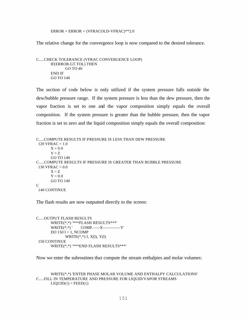
151
ERROR = ERROR + (VFRACOLD-VFRAC)**2.0
The relative change for the convergence loop is now compared to the desired tolerance.
C.....CHECK TOLERANCE (VFRAC CONVERGENCE LOOP) IF(ERROR.GT.TOL) THEN GO TO 40 END IF GO TO 140
The section of code below is only utilized if the system pressure falls outside the
dew/bubble pressure range. If the system pressure is less than the dew pressure, then the
vapor fraction is set to one and the vapor composition simply equals the overall
composition. If the system pressure is greater than the bubble pressure, then the vapor
fraction is set to zero and the liquid composition simply equals the overall composition:
C.....COMPUTE RESULTS IF PRESSURE IS LESS THAN DEW PRESSURE 120 VFRAC = 1.0 X = 0.0 Y = Z GO TO 140 C.....COMPUTE RESULTS IF PRESSURE IS GREATER THAN BUBBLE PRESSURE 130 VFRAC = 0.0 X = Z Y = 0.0 GO TO 140 C 140 CONTINUE
The flash results are now outputted directly to the screen:
C.....OUTPUT FLASH RESULTS WRITE(*,*) '***FLASH RESULTS***' WRITE(*,*) ' COMP.-----X-------------Y' DO 150 I = 1, NCOMP WRITE(*,*) I, X(I), Y(I) 150 CONTINUE WRITE(*,*) '***END FLASH RESULTS***'
Now we enter the subroutines that compute the stream enthalpies and molar volumes:
WRITE(*,*) 'ENTER PHASE MOLAR VOLUME AND ENTHALPY CALCULATIONS' C.....FILL IN TEMPERATURE AND PRESSURE FOR LIQUID/VAPOR STREAMS LIQUID(1) = FEED(1)

152
LIQUID(2) = FEED(2) VAPOR(1) = FEED(1) VAPOR(2) = FEED(2) C.....COMPUTE MOLE FLOW RATES FOR LIQUID/VAPOR STREAMS DO 160 I = 1, NCOMP LIQUID(2+NCOMP+I) = (1.0-VFRAC)*STOT*X(I) VAPOR(2+NCOMP+I) = VFRAC*STOT*Y(I) LIQUID(2+2*NCOMP+I) = FEED(2+2*NCOMP+I) VAPOR(2+2*NCOMP+I) = FEED(2+2*NCOMP+I) 160 CONTINUE C.....COMPUTE MASS FLOW RATES FROM MOLE FLOW RATES FOR LIQUID/VAPOR STREAMS CALL MOLETOMASS(NCOMP, LIQUID) CALL MOLETOMASS(NCOMP, VAPOR) C.....COMPUTE TOTAL MASS FLOW RATE IN LIQUID AND VAPOR STREAMS LTOT = 0.0 VTOT = 0.0 DO 170 I = 1, NCOMP LTOT = LTOT + LIQUID(2+I) VTOT = VTOT + VAPOR(2+I) 170 CONTINUE C.....COMPUTE MOLAR VOLUME AND ENTHALPY OF LIQUID STREAM IF FLOW IS ZERO IF(LTOT.EQ.0) THEN LIQUID(3+3*NCOMP) = 0.0 LIQUID(4+3*NCOMP) = 0.0 GO TO 190 END IF C.....COMPUTE MOLAR VOLUME AND ENTHALPY OF LIQUID STREAM IF FLOW IS NONZERO LIQUID(3+3*NCOMP) = 0.0 CALL LIQUIDMOLARVOLUME(NCOMP, LIQUID, LMOLV) DO 180 I = 1, NCOMP LIQUID(3+3*NCOMP) = LIQUID(3+3*NCOMP) + X(I)*LMOLV(I) 180 CONTINUE C CALL LIQUIDENTHALPY(NCOMP, LIQUID, X, LIQENTH) LIQUID(3*NCOMP+4) = LIQENTH C.....COMPUTE MOLAR VOLUME AND ENTHALPY OF VAPOR STREAM IF FLOW IS ZERO 190 IF(VTOT.EQ.0) THEN VAPOR(3+3*NCOMP) = 0.0 VAPOR(4+3*NCOMP) = 0.0 GO TO 200 END IF C.....COMPUTE MOLAR VOLUME AND ENTHALPY OF VAPOR STREAM IF FLOW IS NONZERO CALL FUGACITY(NCOMP, TEMP, PRES, Y, FUGCOEF, VMOLVOL, ENTHALPY) VAPOR(3+3*NCOMP) = VMOLVOL C CALL VAPORENTHALPY(NCOMP, VAPOR, Y, VAPENTH) VAPOR(3*NCOMP+4) = VAPENTH C 200 RETURN END

153
4.5.19 Driver Program (Program STREAMFLASH)
We use the program STREAMFLASH to drive the VLE flash subroutine. This program
simply includes the necessary input stream information: temperature, pressure, mass flow
rates and degrees of polymerization. The FLASH subroutine then resolves the input
stream into a liquid and vapor stream, while filling in stream properties such as the molar
volume and the enthalpy.
PROGRAM STREAMFLASH C.....PURPOSE: THIS PROGRAM TAKES A STREAM AND PERFORMS A TWO-PHASE C...............TEMPERATURE/PRESSURE FLASH C.....TECHNICALS: DIPPR EQUATION FOR VAPOR PRESSURE C..................DIPPR EQUATION FOR MOLAR VOLUME OF LIQUID SIMPLE SPECIES C..................TAIT/VAN-KREVELEN METHOD FOR MOLAR VOLUME/ENTHALPY OF POLYMERS C..................IDEAL-GAS LAW FOR VAPOR-PHASE FUGACITY COEFFICIENT C..................POLYMER-NRTL EQUATION FOR LIQUID-PHASE ACTIVITY COEFFICIENT C..................POYNTING CORRECTION NOT INCLUDED C.....INPUTS: TEMPERATURE C..............PRESSURE C..............FEEDS (KG/HR) C..............DEGREE OF POLYMERIZATION C..............PHYSICAL PROPERTY PARAMETERS (APPEAR AT END OF CODE) C.....OUPUTS: VAPOR STREAM (TEMPERATURE, PRESSURE, MOLE FLOW, MASS FLOW, C............................DEGREE OF POLYMERIZATION FOR EACH SPECIES, C............................MOLAR VOLUME, MOLAR ENTHALPY) C..............LIQUID STREAM INTEGER NCOMP C*****USER INPUT - NUMBER OF COMPONENTS***************************************** C.....NCOMP = NUMBER OF COMPONENTS IN STREAM PARAMETER (NCOMP = 7) C******************************************************************************* REAL FEED(3*NCOMP+4), LIQUID(3*NCOMP+4), VAPOR(3*NCOMP+4) C.....STREAM VECTOR SET -UP C..........TEMPERATURE(K), PRESSURE (PA) C..........MASS FLOW RATE (KG/S), MOLAR FLOW RATE (MOL/S), C..........DEGREE OF POLYMERIZATION FOR EACH SPECIES, C..........MOLAR VOLUME (M^3/MOL), ENTHALPY (J/MOL) EXTERNAL FLASH C*****USER INPUT - FEED STREAM CHARACTERISTICS********************************** C.....FEED(1) = TEMPERATURE (K) C.....FEED(2) = PRESSURE (PA) FEED(1) = 230.0 + 273.15 FEED(2) = 760.0 * 133.32237 C.....FEED(3-5) = MASS FLOW RATE OF COMPONENT 3-5 (KG/S) FEED(3) = 10.0 FEED(4) = 10.0 FEED(5) = 10.0 FEED(6) = 10.0 FEED(7) = 10.0 FEED(8) = 10.0

154
FEED(9) = 10.0 C.....FEED(9-11) = DEGREE OF POLYMERIZATION OF COMPONENT 9-11 FEED(17) = 1.0 FEED(18) = 1.0 FEED(19) = 1.0 FEED(20) = 1.0 FEED(21) = 1.0 FEED(22) = 1.0 FEED(23) = 25.0 C******************************************************************************* CALL FLASH(NCOMP, FEED, LIQUID, VAPOR) C END
We feed 10.0 kg/s of each component. The number-average degree of polymerization of
the polymer is 25. The flash takes place at 230 °C and 1 atm.
4.6 Performance of Simulation
Table 4.14 shows the major simulation results for an example flash calculation.
Table 4.14. Example flash calculation - physical property system predictions
Output Feed Liquid Vapor
Water mass flow
rate (kg/s) 1.0000E+01 7.3646E-02 9.9264E+00
Caprolactam mass
flow rate (kg/s) 1.0000E+01 3.6475E+00 6.3525E+00
Cyclic dimer mass
flow rate (kg/s) 1.0000E+01 1.0000E+01 0.0000E+00
Aminocaproic acid
mass flow rate
(kg/s)
1.0000E+01 1.0000E+01 0.0000E+00
Acetic acid mass
flow rate (kg/s) 1.0000E+01 1.4660E-01 9.8534E+00
Cyclohexylamine
mass flow rate
(kg/s)
1.0000E+01 2.5047E-01 9.7495E+00

155
Nylon-6 mass flow
rate (kg/s) 1.0000E+01 1.0000E+01 0.0000E+00
Volumetric flow
rate (m3 /s) 3.0095E-02 3.5899E+01
Mass enthalpy
(J/kg) -1.9876E+06 -6.0292E+06
The non-volatile species, nylon-6, cyclic dimer, and aminocaproic acid, remain in the
liquid phase.
4.7 Conclusions
We have shown how to implement the activity coefficient approach in describing the
physical properties of nylon-6 reaction mixtures. The FORTRAN code easily handles
changes in simulation, including the modification of chemical species present, changes in
temperature or pressure, and changes in physical property models and parameters. The
physical property system is suitable for describing non- ideal vapor/liquid mixtures
appearing in nearly all hydrolytic step-growth polymerizations.
The hydrolytic polymerization of nylon-6 typically does not involve high-pressure phase
equilibrium; therefore, the ideal gas equation of state is suitable for describing the vapor
phase. Also, the POLYNRTL activity coefficient model can moderately high degrees
non- ideal behavior in the liquid phase.
As was mentioned previously, we do not recommend extrapolation using empirical
models. Model developers should always seek to validate their models within the
temperature-pressure ranges of interest.

156
4.8 Nomenclature
Symbol Description Units
a Carreau-Yasuda parameter or Mark-Houwink exponent Unitless
Ta Temperature shift factor Unitless
,p polyc Polymer heat capacity J/kmol-seg-K
,p ic○ Ideal-gas heat capacity for species i J/kmol-K
FAV Formic-acid viscosity Unitless
H Flow activation energy J/kmol Eh Excess enthalpy of mixing J/kmol
,f ih○ Ideal-gas enthalpy of formation for species i J/kmol
vih Enthalpy of vaporization of species i J/kmol
Lh Liquid mixture enthalpy J/kmol
,L ih○ Ideal- liquid enthalpy of species i J/kmol
,L polyh○ Ideal-polymer enthalpy J/kmol-seg
Vh Vapor mixture enthalpy J/kmol
rxnh∆ Enthalpy of reaction J/kmol
,refT polyh○ Reference ideal-polymer enthalpy at Tref J/kmol-seg
,V ih○ Ideal-gas enthalpy of species i J/kmol
K Mark-Houwink constant ml/g
vM Viscosity-average molecular weight kg/kmol
wM Weight-average molecular weight kg/kmol
P Pressure Pa s
iP Critical pressure of species i Pa
siP Vapor pressure of species i Pa
R Ideal-gas law constant J/kmol-K
T Temperature K

157
Tc Critical temperature K
Tref Reference temperature K
xi Liquid mole fraction of species i Unitless
yi Vapor mole fraction of species i Unitless
iγ Activity coefficient of species i Unitless
γ& Shear rate 1/s
η Non-Newtonian steady-shear viscosity Pa-s
0η Zero-shear viscosity Pa-s
[ ]η Intrinsic viscosity ml/g
iv Liquid-molar volume of species i m3/mol
Lv Mixture liquid molar volume m3/mol
,V iv Vapor-molar volume of species i m3/mol
ητ Carreau-Yasuda relaxation time s

158
4.9 Appendix - FORTRAN 77 Code (DIGITAL Visual FORTRAN
6.0)
PROGRAM STREAMFLASH C.....PURPOSE: THIS PROGRAM TAKES A STREAM AND PERFORMS A TWO-PHASE C...............TEMPERATURE/PRESSURE FLASH C.....TECHNICALS: DIPPR EQUATION FOR VAPOR PRESSURE C..................DIPPR EQUATION FOR MOLAR VOLUME OF LIQUID SIMPLE SPECIES C..................TAIT/VAN-KREVELEN METHOD FOR MOLAR VOLUME/ENTHALPY OF POLYMERS C..................IDEAL-GAS LAW FOR VAPOR-PHASE FUGACITY COEFFICIENT C..................POLYMER-NRTL EQUATION FOR LIQUID-PHASE ACTIVITY COEFFICIENT C..................POYNTING CORRECTION NOT INCLUDED C.....INPUTS: TEMPERATURE C..............PRESSURE C..............FEEDS (KG/HR) C............. .DEGREE OF POLYMERIZATION C..............PHYSICAL PROPERTY PARAMETERS (APPEAR AT END OF CODE) C.....OUPUTS: VAPOR STREAM (TEMPERATURE, PRESSURE, MOLE FLOW, MASS FLOW, C............................DEGREE OF POLYMERIZATION FOR EACH SPECIES, C............................MOLAR VOLUME, MOLAR ENTHALPY) C..............LIQUID STREAM INTEGER NCOMP C*****USER INPUT - NUMBER OF COMPONENTS***************************************** C.....NCOMP = NUMBER OF COMPONENTS IN STREAM * PARAMETER (NCOMP = 7) C******************************************************************************* REAL FEED(3*NCOMP+4), LIQUID(3*NCOMP+4), VAPOR(3*NCOMP+4) REAL TOTMOLLIQ, TOTMOLVAP, TOTMASLIQ, TOTMASVAP, ENTHALPYL REAL ENTHALPYV, MOLARVOLUMEL, MOLARVOLUMEV C.....STREAM VECTOR SET -UP C..........TEMPERATURE(K), PRESSURE (PA) C..........MASS FLOW RATE (KG/S), MOLAR FLOW RATE (MOL/S), C..........DEGREE OF POLYMERIZATION FOR EACH SPECIES, C..........MOLAR VOLUME (M^3/MOL), ENTHALPY (J/MOL) EXTERNAL FLASH C*****USER INPUT - FEED STREAM CHARACTERISTICS********************************** C.....FEED(1) = TEMPERATURE (K) * C.....FEED(2) = PRESSURE (PA) * FEED(1) = 230.0 + 273.15 FEED(2) = 760.0 * 133.32237 C.....FEED(3-5) = MASS FLOW RATE OF COMPONENT 3-5 (KG/S) * FEED(3) = 10.0 FEED(4) = 10.0 FEED(5) = 10.0 FEED(6) = 10.0 FEED(7) = 10.0 FEED(8) = 10.0 FEED(9) = 10.0 C.....FEED(9-11) = DEGREE OF POLYMERIZATION OF COMPONENT 9-11 * FEED(17) = 1.0 FEED(18) = 1.0 FEED(19) = 1.0
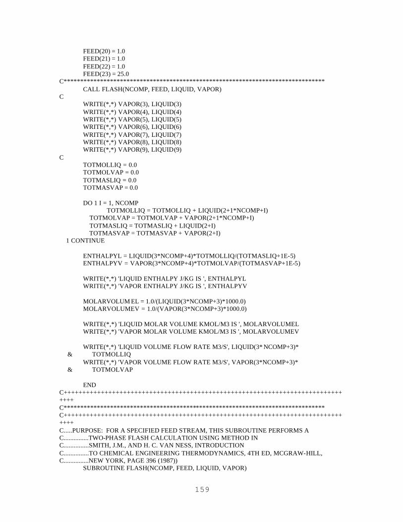
159
FEED(20) = 1.0 FEED(21) = 1.0 FEED(22) = 1.0 FEED(23) = 25.0 C******************************************************************************* CALL FLASH(NCOMP, FEED, LIQUID, VAPOR) C WRITE(*,*) VAPOR(3), LIQUID(3) WRITE(*,*) VAPOR(4), LIQUID(4) WRITE(*,*) VAPOR(5), LIQUID(5) WRITE(*,*) VAPOR(6), LIQUID(6) WRITE(*,*) VAPOR(7), LIQUID(7) WRITE(*,*) VAPOR(8), LIQUID(8) WRITE(*,*) VAPOR(9), LIQUID(9) C TOTMOLLIQ = 0.0 TOTMOLVAP = 0.0 TOTMASLIQ = 0.0 TOTMASVAP = 0.0 DO 1 I = 1, NCOMP TOTMOLLIQ = TOTMOLLIQ + LIQUID(2+1*NCOMP+I) TOTMOLVAP = TOTMOLVAP + VAPOR(2+1*NCOMP+I) TOTMASLIQ = TOTMASLIQ + LIQUID(2+I) TOTMASVAP = TOTMASVAP + VAPOR(2+I) 1 CONTINUE ENTHALPYL = LIQUID(3*NCOMP+4)*TOTMOLLIQ/(TOTMASLIQ+1E-5) ENTHALPYV = VAPOR(3*NCOMP+4)*TOTMOLVAP/(TOTMASVAP+1E-5) WRITE(*,*) 'LIQUID ENTHALPY J/KG IS ', ENTHALPYL WRITE(*,*) 'VAPOR ENTHALPY J/KG IS ', ENTHALPYV MOLARVOLUM EL = 1.0/(LIQUID(3*NCOMP+3)*1000.0) MOLARVOLUMEV = 1.0/(VAPOR(3*NCOMP+3)*1000.0) WRITE(*,*) 'LIQUID MOLAR VOLUME KMOL/M3 IS ', MOLARVOLUMEL WRITE(*,*) 'VAPOR MOLAR VOLUME KMOL/M3 IS ', MOLARVOLUMEV WRITE(*,*) 'LIQUID VOLUME FLOW RATE M3/S', LIQUID(3* NCOMP+3)* & TOTMOLLIQ WRITE(*,*) 'VAPOR VOLUME FLOW RATE M3/S', VAPOR(3*NCOMP+3)* & TOTMOLVAP END C+++++++++++++++++++++++++++++++++++++++++++++++++++++++++++++++++++++++++++++++ C******************************************************************************* C+++++++++++++++++++++++++++++++++++++++++++++++++++++++++++++++++++++++++++++++ C.....PURPOSE: FOR A SPECIFIED FEED STREAM, THIS SUBROUTINE PERFORMS A C...............TWO-PHASE FLASH CALCULATION USING METHOD IN C...............SMITH, J.M., AND H. C. VAN NESS, INTRODUCTION C...............TO CHEMICAL ENGINEERING THERMODYNAMICS, 4TH ED, MCGRAW-HILL, C...............NEW YORK, PAGE 396 (1987)) SUBROUTINE FLASH(NCOMP, FEED, LIQUID, VAPOR)
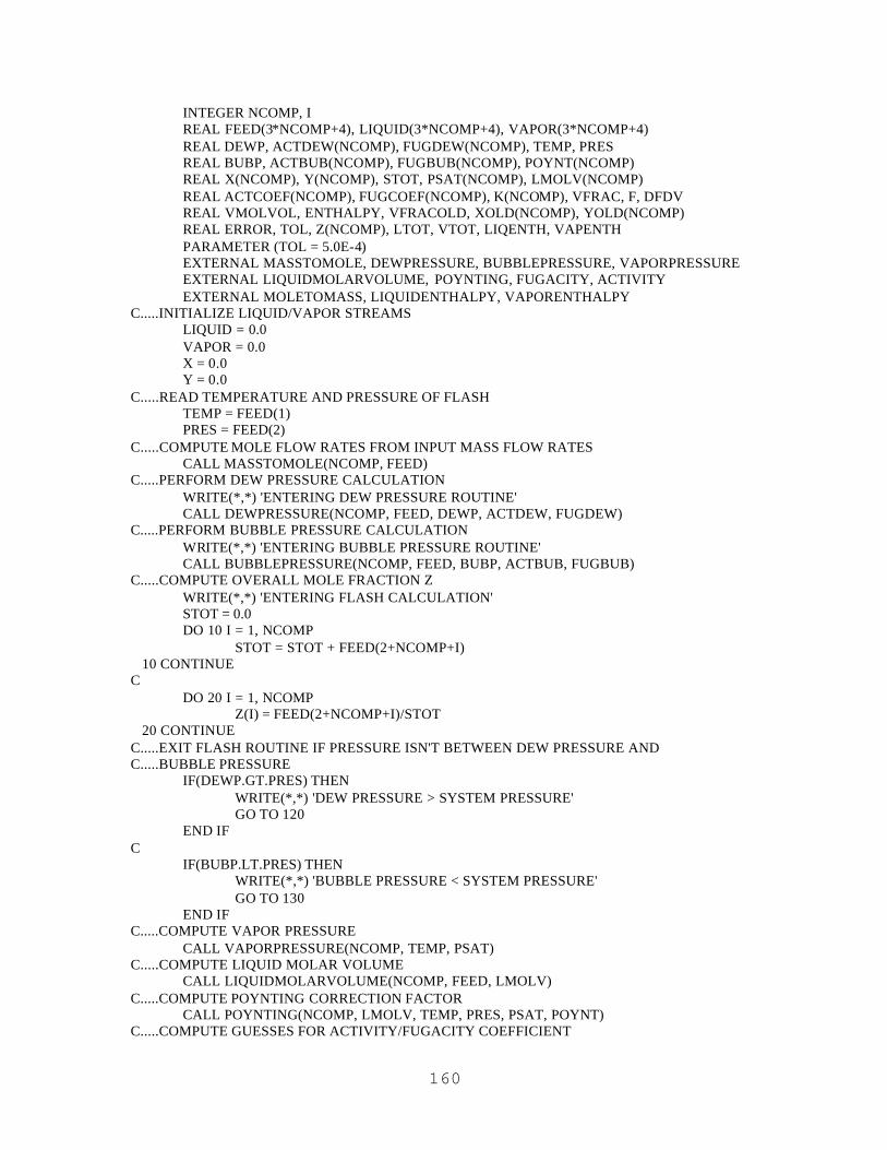
160
INTEGER NCOMP, I REAL FEED(3*NCOMP+4), LIQUID(3*NCOMP+4), VAPOR(3*NCOMP+4) REAL DEWP, ACTDEW(NCOMP), FUGDEW(NCOMP), TEMP, PRES REAL BUBP, ACTBUB(NCOMP), FUGBUB(NCOMP), POYNT(NCOMP) REAL X(NCOMP), Y(NCOMP), STOT, PSAT(NCOMP), LMOLV(NCOMP) REAL ACTCOEF(NCOMP), FUGCOEF(NCOMP), K(NCOMP), VFRAC, F, DFDV REAL VMOLVOL, ENTHALPY, VFRACOLD, XOLD(NCOMP), YOLD(NCOMP) REAL ERROR, TOL, Z(NCOMP), LTOT, VTOT, LIQENTH, VAPENTH PARAMETER (TOL = 5.0E-4) EXTERNAL MASSTOMOLE, DEWPRESSURE, BUBBLEPRESSURE, VAPORPRESSURE EXTERNAL LIQUIDMOLARVOLUME, POYNTING, FUGACITY, ACTIVITY EXTERNAL MOLETOMASS, LIQUIDENTHALPY, VAPORENTHALPY C.....INITIALIZE LIQUID/VAPOR STREAMS LIQUID = 0.0 VAPOR = 0.0 X = 0.0 Y = 0.0 C.....READ TEMPERATURE AND PRESSURE OF FLASH TEMP = FEED(1) PRES = FEED(2) C.....COMPUTE MOLE FLOW RATES FROM INPUT MASS FLOW RATES CALL MASSTOMOLE(NCOMP, FEED) C.....PERFORM DEW PRESSURE CALCULATION WRITE(*,*) 'ENTERING DEW PRESSURE ROUTINE' CALL DEWPRESSURE(NCOMP, FEED, DEWP, ACTDEW, FUGDEW) C.....PERFORM BUBBLE PRESSURE CALCULATION WRITE(*,*) 'ENTERING BUBBLE PRESSURE ROUTINE' CALL BUBBLEPRESSURE(NCOMP, FEED, BUBP, ACTBUB, FUGBUB) C.....COMPUTE OVERALL MOLE FRACTION Z WRITE(*,*) 'ENTERING FLASH CALCULATION' STOT = 0.0 DO 10 I = 1, NCOMP STOT = STOT + FEED(2+NCOMP+I) 10 CONTINUE C DO 20 I = 1, NCOMP Z(I) = FEED(2+NCOMP+I)/STOT 20 CONTINUE C.....EXIT FLASH ROUTINE IF PRESSURE ISN'T BETWEEN DEW PRESSURE AND C.....BUBBLE PRESSURE IF(DEWP.GT.PRES) THEN WRITE(*,*) 'DEW PRESSURE > SYSTEM PRESSURE' GO TO 120 END IF C IF(BUBP.LT.PRES) THEN WRITE(*,*) 'BUBBLE PRESSURE < SYSTEM PRESSURE' GO TO 130 END IF C.....COMPUTE VAPOR PRESSURE CALL VAPORPRESSURE(NCOMP, TEMP, PSAT) C.....COMPUTE LIQUID MOLAR VOLUME CALL LIQUIDMOLARVOLUME(NCOMP, FEED, LMOLV) C.....COMPUTE POYNTING CORRECTION FACTOR CALL POYNTING(NCOMP, LMOLV, TEMP, PRES, PSAT, POYNT) C.....COMPUTE GUESSES FOR ACTIVITY/FUGACITY COEFFICIENT

161
DO 30 I = 1, NCOMP ACTCOEF(I) = (ACTBUB(I)-ACTDEW(I))*(PRES -DEWP)/(BUBP-DEWP)+ & ACTDEW(I) FUGCOEF(I) = (FUGBUB(I)-FUGDEW(I))*(PRES-DEWP)/(BUBP-DEWP)+ & FUGDEW(I) 30 CONTINUE C.....COMPUTE GUESS FOR VAPOR MOLE FRACTION VFRAC = (BUBP-PRES)/(BUBP-DEWP) C.....COMPUTE K VALUES FOR EACH COMPONENT 40 DO 50 I = 1, NCOMP K(I) = ACT COEF(I)*PSAT(I)*POYNT(I)/FUGCOEF(I)/PRES 50 CONTINUE C.....COMPUTE F-VALUE FOR NEWTON ITERATION F = 0.0 DO 60 I = 1, NCOMP F = F + Z(I)*(K(I)-1.0)/(1.0 + VFRAC*(K(I)-1.0)) 60 CONTINUE C.....COMPUTE DFDV-VALUE FOR NEWTON ITERATION DFDV = 0.0 DO 70 I = 1, NCOMP DFDV = DFDV + Z(I)*((K(I)-1.0)**2.0)/ & ((1.0+VFRAC*(K(I)-1.0))**2.0) 70 CONTINUE DFDV = -1.0*DFDV C VFRACOLD = VFRAC XOLD = X YOLD = Y C.....UPDATE NEWTON ITERATION FOR VAPOR MOLE FRACTION VFRAC = VFRAC - F/DFDV C DO 80 I = 1, NCOMP X(I) = Z(I)/(1.0 + VFRAC*(K(I)-1.0)) Y(I) = K(I)*X(I) 80 CONTINUE C.....COMPUTE FUGACITY COEFFICIENT CALL FUGACITY(NCOMP, TEMP, PRES, Y, FUGCOEF, VMOLVOL, ENTHALPY) C.....COMPUTE ACTIVITY COEFFICIENT CALL ACTIVITY(NCOMP, FEED, X, ACTCOEF) C.....COMPUTE CHANGES IN VFRAC, X, AND Y ERROR = 0.0 DO 90 I = 1, NCOMP ERROR = ERROR + (XOLD(I)-X(I))**2.0 + (YOLD(I)-Y(I))**2.0 90 CONTINUE ERROR = ERROR + (VFRACOLD-VFRAC)**2.0 C.....CHECK TOLERANCE (VFRAC CONVERGENCE LOOP) IF(ERROR.GT.TOL) THEN GO TO 40 END IF GO TO 140 C.....COMPUTE RESULTS IF PRESSURE IS LESS THAN DEW PRESSURE 120 VFRAC = 1.0 X = 0.0 Y = Z GO TO 140 C.....COMPUTE RESULTS IF PRESSURE IS GREATER THAN BUBBLE PRESSURE
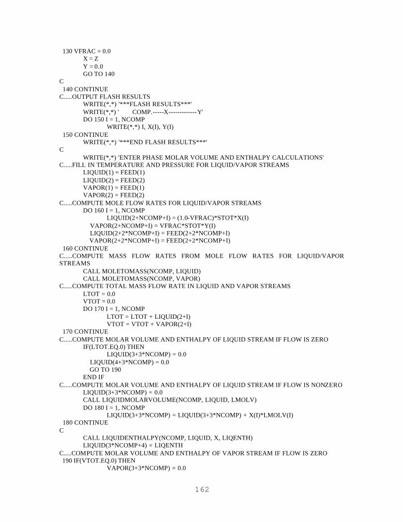
162
130 VFRAC = 0.0 X = Z Y = 0.0 GO TO 140 C 140 CONTINUE C.....OUTPUT FLASH RESULTS WRITE(*,*) '***FLASH RESULTS***' WRITE(*,*) ' COMP.-----X-------------Y' DO 150 I = 1, NCOMP WRITE(*,*) I, X(I), Y(I) 150 CONTINUE WRITE(*,*) '***END FLASH RESULTS***' C WRITE(*,*) 'ENTER PHASE MOLAR VOLUME AND ENTHALPY CALCULATIONS' C.....FILL IN TEMPERATURE AND PRESSURE FOR LIQUID/VAPOR STREAMS LIQUID(1) = FEED(1) LIQUID(2) = FEED(2) VAPOR(1) = FEED(1) VAPOR(2) = FEED(2) C.....COMPUTE MOLE FLOW RATES FOR LIQUID/VAPOR STREAMS DO 160 I = 1, NCOMP LIQUID(2+NCOMP+I) = (1.0-VFRAC)*STOT*X(I) VAPOR(2+NCOMP+I) = VFRAC*STOT*Y(I) LIQUID(2+2*NCOMP+I) = FEED(2+2*NCOMP+I) VAPOR(2+2*NCOMP+I) = FEED(2+2*NCOMP+I) 160 CONTINUE C.....COMPUTE MASS FLOW RATES FROM MOLE FLOW RATES FOR LIQUID/VAPOR STREAMS CALL MOLETOMASS(NCOMP, LIQUID) CALL MOLETOMASS(NCOMP, VAPOR) C.....COMPUTE TOTAL MASS FLOW RATE IN LIQUID AND VAPOR STREAMS LTOT = 0.0 VTOT = 0.0 DO 170 I = 1, NCOMP LTOT = LTOT + LIQUID(2+I) VTOT = VTOT + VAPOR(2+I) 170 CONTINUE C.....COMPUTE MOLAR VOLUME AND ENTHALPY OF LIQUID STREAM IF FLOW IS ZERO IF(LTOT.EQ.0) THEN LIQUID(3+3*NCOMP) = 0.0 LIQUID(4+3*NCOMP) = 0.0 GO TO 190 END IF C.....COMPUTE MOLAR VOLUME AND ENTHALPY OF LIQUID STREAM IF FLOW IS NONZERO LIQUID(3+3*NCOMP) = 0.0 CALL LIQUIDMOLARVOLUME(NCOMP, LIQUID, LMOLV) DO 180 I = 1, NCOMP LIQUID(3+3*NCOMP) = LIQUID(3+3*NCOMP) + X(I)*LMOLV(I) 180 CONTINUE C CALL LIQUIDENTHALPY(NCOMP, LIQUID, X, LIQENTH) LIQUID(3*NCOMP+4) = LIQENTH C.....COMPUTE MOLAR VOLUME AND ENTHALPY OF VAPOR STREAM IF FLOW IS ZERO 190 IF(VTOT.EQ.0) THEN VAPOR(3+3*NCOMP) = 0.0

163
VAPOR(4+3*NCOMP) = 0.0 GO TO 200 END IF C.....COMPUTE MOLAR VOLUME AND ENTHALPY OF VAPOR STREAM IF FLOW IS NONZERO CALL FUGACITY(NCOMP, TEMP, PRES, Y, FUGCOEF, VMOLVOL, ENTHALPY) VAPOR(3+3*NCOMP) = VMOLVOL C CALL VAPORENTHALPY(NCOMP, VAPOR, Y, VAPENTH) VAPOR(3*NCOMP+4) = VAPENTH C 200 RETURN END C+++++++++++++++++++++++++++++++++++++++++++++++++++++++++++++++++++++++++++++++ C******************************************************************************* C+++++++++++++++++++++++++++++++++++++++++++++++++++++++++++++++++++++++++++++++ C.....PURPOSE: FOR A SPECIFIED TEMPERATURE AND FEED, THIS C...............SUBROUTINE DOES A DEW-PRESSURE CALCULATION USING THE C...............METHOD OUTLINED IN SMITH, J.M., AND H. C. VAN NESS, INTRODUCTION C...............TO CHEMICAL ENGINEERING THERMODYNAMICS, 4TH ED, MCGRAW-HILL, C...............NEW YORK, PAGE 382 (1987) SUBROUTINE DEWPRESSURE(NCOMP, STREAM, DEWP, ACTDEW, FUGDEW) INTEGER NCOMP, I REAL STREAM(3*NCOMP+4), ACTDEW(NCOMP), FUGDEW(NCOMP), DEWP REAL PSAT(NCOMP), LMOLV(NCOMP), Y(NCOMP), TEMP, STOT REAL X(NCOMP), VMOLVOL, ENTHALPY, POYNT(NCOMP), ACTOLD(NCOMP) REAL ERROR1, ERROR2, DEWPOLD, TOL1, TOL2 PARAMETER (TOL1 = 10.0, TOL2 = 1.0E-5) EXTERNAL VAPORPRESSURE, LIQUIDMOLARVOLUME, ACTIVITY, NORMALIZE EXTERNAL FUGACITY, POYNTING C.....READ TEMPERATURE TEMP = STREAM(1) C.....SET Y = Z STOT = 0.0 DO 10 I = 1, NCOMP STOT = STOT + STREAM(2+NCOMP+I) 10 CONTINUE C DO 20 I = 1, NCOMP Y(I) = STREAM(2+NCOMP+I)/STOT 20 CONTINUE C.....SET ACTIVITY/FUGACITY COEFFICIENTS EQUAL TO ONE FUGDEW = 1.0 ACTDEW = 1.0 C.....COMPUTE VAPOR PRESSURE CALL VAPORPRESSURE(NCOMP, TEMP, PSAT) C.....COMPUTE LIQUID MOLAR VOLUMES CALL LIQUIDMOLARVOLUME(NCOMP, STREAM, LMOLV) C.....COMPUTE DEW PRESSURE DEWP = 0.0 DO 30 I = 1, NCOMP DEWP = DEWP + Y(I)*FUGDEW(I)/ACTDEW(I)/PSAT(I) 30 CONTINUE DEWP = 1.0/DEWP C.....COMPUTE X
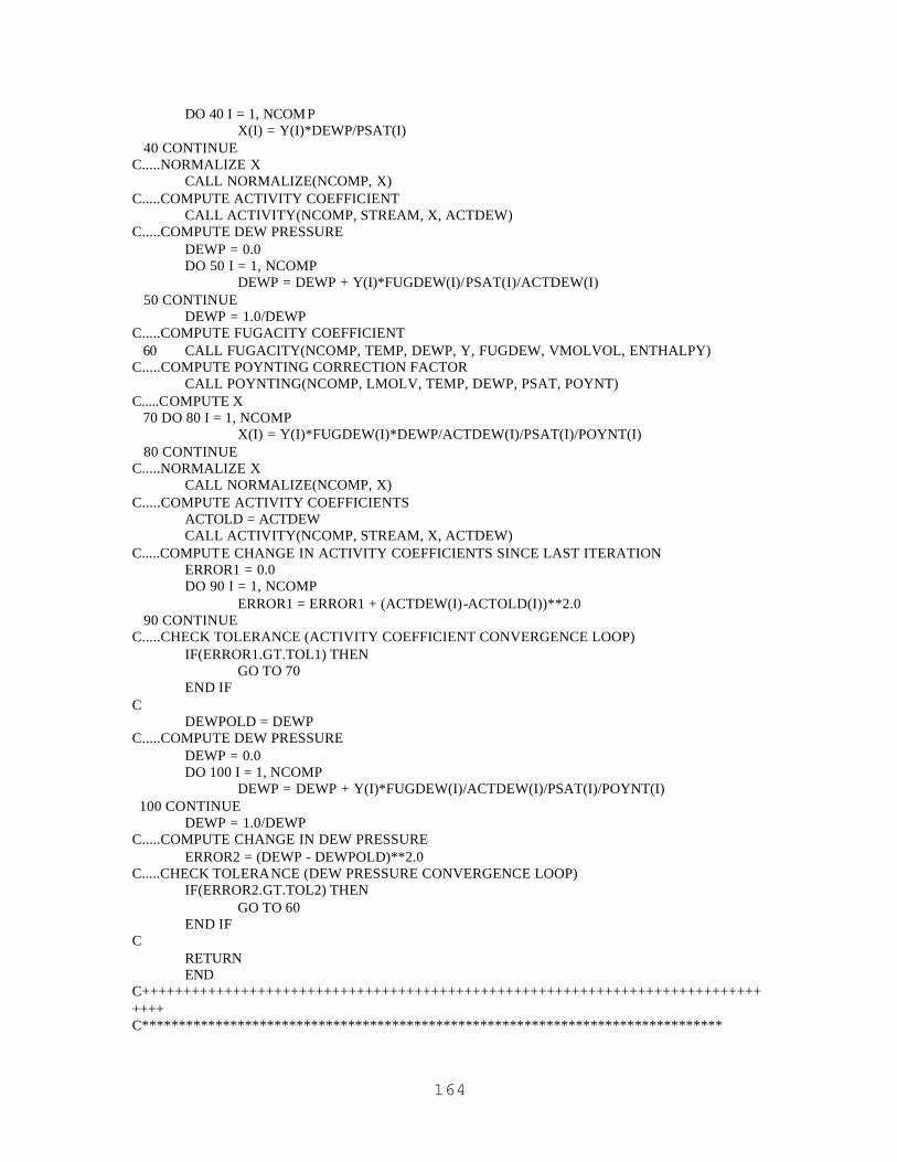
164
DO 40 I = 1, NCOMP X(I) = Y(I)*DEWP/PSAT(I) 40 CONTINUE C.....NORMALIZE X CALL NORMALIZE(NCOMP, X) C.....COMPUTE ACTIVITY COEFFICIENT CALL ACTIVITY(NCOMP, STREAM, X, ACTDEW) C.....COMPUTE DEW PRESSURE DEWP = 0.0 DO 50 I = 1, NCOMP DEWP = DEWP + Y(I)*FUGDEW(I)/PSAT(I)/ACTDEW(I) 50 CONTINUE DEWP = 1.0/DEWP C.....COMPUTE FUGACITY COEFFICIENT 60 CALL FUGACITY(NCOMP, TEMP, DEWP, Y, FUGDEW, VMOLVOL, ENTHALPY) C.....COMPUTE POYNTING CORRECTION FACTOR CALL POYNTING(NCOMP, LMOLV, TEMP, DEWP, PSAT, POYNT) C.....COMPUTE X 70 DO 80 I = 1, NCOMP X(I) = Y(I)*FUGDEW(I)*DEWP/ACTDEW(I)/PSAT(I)/POYNT(I) 80 CONTINUE C.....NORMALIZE X CALL NORMALIZE(NCOMP, X) C.....COMPUTE ACTIVITY COEFFICIENTS ACTOLD = ACTDEW CALL ACTIVITY(NCOMP, STREAM, X, ACTDEW) C.....COMPUTE CHANGE IN ACTIVITY COEFFICIENTS SINCE LAST ITERATION ERROR1 = 0.0 DO 90 I = 1, NCOMP ERROR1 = ERROR1 + (ACTDEW(I)-ACTOLD(I))**2.0 90 CONTINUE C.....CHECK TOLERANCE (ACTIVITY COEFFICIENT CONVERGENCE LOOP) IF(ERROR1.GT.TOL1) THEN GO TO 70 END IF C DEWPOLD = DEWP C.....COMPUTE DEW PRESSURE DEWP = 0.0 DO 100 I = 1, NCOMP DEWP = DEWP + Y(I)*FUGDEW(I)/ACTDEW(I)/PSAT(I)/POYNT(I) 100 CONTINUE DEWP = 1.0/DEWP C.....COMPUTE CHANGE IN DEW PRESSURE ERROR2 = (DEWP - DEWPOLD)**2.0 C.....CHECK TOLERANCE (DEW PRESSURE CONVERGENCE LOOP) IF(ERROR2.GT.TOL2) THEN GO TO 60 END IF C RETURN END C+++++++++++++++++++++++++++++++++++++++++++++++++++++++++++++++++++++++++++++++ C*******************************************************************************

165
C+++++++++++++++++++++++++++++++++++++++++++++++++++++++++++++++++++++++++++++++ C.....PURPOSE: FOR A SPECIFIED TEMPERATURE AND FEED, THIS C...............SUBROUTINE DOES A BUBBLE-PRESSURE CALCULATION USING THE C...............METHOD OUTLINED IN SMITH, J.M., AND H. C. VAN NESS, INTRODUCTION C...............TO CHEMICAL ENGINEERING THERMODYNAMICS, 4TH ED, MCGRAW-HILL, C...............NEW YORK, PAGE 383 (1987) SUBROUTINE BUBBLEPRESSURE(NCOMP, STREAM, BUBP, ACTBUB, FUGBUB) INTEGER NCOMP, I REAL STREAM(3* NCOMP+4), BUBP, ACTBUB(NCOMP), FUGBUB(NCOMP) REAL PSAT(NCOMP), TEMP, LMOLV(NCOMP), POYNT(NCOMP), STOT REAL X(NCOMP), Y(NCOMP), VMOLVOL, ENTHALPY, BUBPOLD, ERROR, TOL PARAMETER (TOL = 1.0E-05) EXTERNAL POYNTING, VAPORPRESSURE, FUGACITY, ACTIVITY, NORMALIZE C.....READ TEMPERATURE TEMP = STREAM(1) C.....SET X = Z STOT = 0.0 DO 10 I = 1, NCOMP STOT = STOT + STREAM(2+NCOMP+I) 10 CONTINUE C DO 20 I = 1, NCOMP X(I) = STREAM(2+NCOMP+I)/STOT 20 CONTINUE C.....SET FUGACITY COEFFICIENTS EQUAL TO ONE FUGBUB = 1.0 C.....COMPUTE VAPOR PRESSURE CALL VAPORPRESSURE(NCOMP, TEMP, PSAT) C.....COMPUTE LIQUID MOLAR VOLUME CALL LIQUIDMOLARVOLUME(NCOMP, STREAM, LMOLV) C.....COMPUTE ACTIVITY COEFFICIENTS CALL ACTIVITY(NCOMP, STREAM, X, ACTBUB) C.....COMPUTE BUBBLE PRESSURE BUBP = 0.0 DO 30 I = 1, NCOMP BUBP = BUBP + X(I)*ACTBUB(I)*PSAT(I)/FUGBUB(I) 30 CONTINUE C.....COMPUTE POYNTING CORRECTION FACTORS 40 CALL POYNTING(NCOMP, LMOLV, TEMP, BUBP, PSAT, POYNT) C.....COMPUTE Y DO 50 I = 1, NCOMP Y(I) = X(I)*ACTBUB(I)*PSAT(I)*POYNT(I)/FUGBUB(I)/BUBP 50 CONTINUE C.....NORMALIZE Y CALL NORMALIZE(NCOMP, Y) C.....COMPUTE FUGACITY COEFFICIENTS CALL FUGACITY(NCOMP, TEMP, BUBP, Y, FUGBUB, VMOLVOL, ENTHALPY) C BUBPOLD = BUBP C.....COMPUTE BUBBLE PRESSURE BUBP = 0.0 DO 60 I = 1, NCOMP BUBP = BUBP + X(I)*ACTBUB(I)*PSAT(I)*POYNT(I)/FUGBUB(I) 60 CONTINUE C.....COMPUTE CHANGE IN BUBBLE PRESSURE
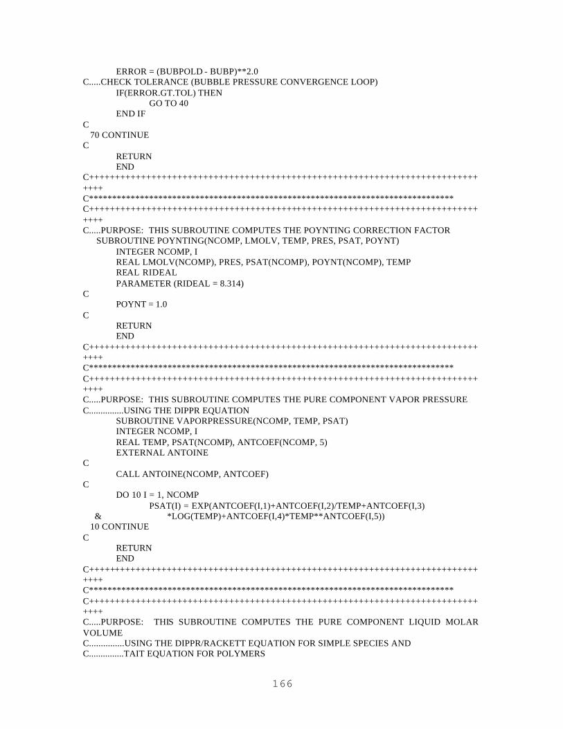
166
ERROR = (BUBPOLD - BUBP)**2.0 C.....CHECK TOLERANCE (BUBBLE PRESSURE CONVERGENCE LOOP) IF(ERROR.GT.TOL) THEN GO TO 40 END IF C 70 CONTINUE C RETURN END C+++++++++++++++++++++++++++++++++++++++++++++++++++++++++++++++++++++++++++++++ C******************************************************************************* C+++++++++++++++++++++++++++++++++++++++++++++++++++++++++++++++++++++++++++++++ C.....PURPOSE: THIS SUBROUTINE COMPUTES THE POYNTING CORRECTION FACTOR SUBROUTINE POYNTING(NCOMP, LMOLV, TEMP, PRES, PSAT, POYNT) INTEGER NCOMP, I REAL LMOLV(NCOMP), PRES, PSAT(NCOMP), POYNT(NCOMP), TEMP REAL RIDEAL PARAMETER (RIDEAL = 8.314) C POYNT = 1.0 C RETURN END C+++++++++++++++++++++++++++++++++++++++++++++++++++++++++++++++++++++++++++++++ C******************************************************************************* C+++++++++++++++++++++++++++++++++++++++++++++++++++++++++++++++++++++++++++++++ C.....PURPOSE: THIS SUBROUTINE COMPUTES THE PURE COMPONENT VAPOR PRESSURE C...............USING THE DIPPR EQUATION SUBROUTINE VAPORPRESSURE(NCOMP, TEMP, PSAT) INTEGER NCOMP, I REAL TEMP, PSAT(NCOMP), ANTCOEF(NCOMP, 5) EXTERNAL ANTOINE C CALL ANTOINE(NCOMP, ANTCOEF) C DO 10 I = 1, NCOMP PSAT(I) = EXP(ANTCOEF(I,1)+ANTCOEF(I,2)/TEMP+ANTCOEF(I,3) & *LOG(TEMP)+ANTCOEF(I,4)*TEMP**ANTCOEF(I,5)) 10 CONTINUE C RETURN END C+++++++++++++++++++++++++++++++++++++++++++++++++++++++++++++++++++++++++++++++ C******************************************************************************* C+++++++++++++++++++++++++++++++++++++++++++++++++++++++++++++++++++++++++++++++ C.....PURPOSE: THIS SUBROUTINE COMPUTES THE PURE COMPONENT LIQUID MOLAR VOLUME C...............USING THE DIPPR/RACKETT EQUATION FOR SIMPLE SPECIES AND C...............TAIT EQUATION FOR POLYMERS

167
SUBROUTINE LIQUIDMOLARVOLUME(NCOMP, STREAM, LMOLV) INTEGER NCOMP, I REAL LMOLV(NCOMP), MOLV(NCOMP, 5), TEMP, RIDEAL REAL STREAM(3*NCOMP+4), PRES, MW(NCOMP) PARAMETER (RIDEAL = 8.314) EXTERNAL MOLVOLP, MOLECULARWEIGHT C TEMP = STREAM(1) PRES = STREAM(2) C CALL MOLVOLP(NCOMP, MOLV) CALL MOLECULARWEIGHT(NCOMP, MW) C DO 10 I = 1, NCOMP IF(STREAM(2+2*NCOMP+I).EQ.1.0) THEN LMOLV(I) = (MOLV(I,2)**(1.0+(1.0-TEMP/MOLV(I,3)) & **MOLV(I,4)))/MOLV(I,1) ELSE LMOLV(I) = ((MOLV(I,1) + MOLV(I,2)*(TEMP-273.15) + & MOLV(I,3)*(TEMP-273.15)**2.0) * & (1.0 - 0.0894*LOG(1.0 + PRES/(MOLV(I,4)* & EXP(-1.0*MOLV(I,5)*(TEMP-273.15)))))) * & MW(I) * STREAM(2+2*NCOMP+I) END IF 10 CONTINUE C RETURN END C+++++++++++++++++++++++++++++++++++++++++++++++++++++++++++++++++++++++++++++++ C******************************************************************************* C+++++++++++++++++++++++++++++++++++++++++++++++++++++++++++++++++++++++++++++++ C.....PURPOSE: COMPUTE LIQUID-PHASE ACTIVITY COEFFICIENT USING C...............POLYNRTL ACTIVITY COEFFICIENT MODEL C...............(CHEN, C. C., "A SEGMENT-BASED LOCAL COMPOSITION MODEL FOR THE C................GIBBS ENERGY OF POLYMER SOLUTIONS," FLUID PHASE EQUILIBRIA, C................83, PAGES 301-312 (1993) SUBROUTINE ACTIVITY(NCOMP, STREAM, X, ACTCOEF) INTEGER NCOMP, I REAL STREAM(3*NCOMP+4), X(NCOMP), ACTCOEF(NCOMP), XSEG(NCOMP) REAL BININTPAR(NCOMP*NCOMP, 8), TEMP, DP(NCOMP), XSEGTOT REAL PHIOVERR, FLORY(NCOMP), NRTL(NCOMP) REAL SUM1, SUM2, SUM3, SUM4, SUM5, SUM6 EXTERNAL BINARY C.....READ TEMPERATURE TEMP = STREAM(1) C.....READ DEGREE OF POLYMERIZATION FOR ALL SPECIES DO 10 I = 1, NCOMP DP(I) = STREAM(2+2*NCOMP+I) 10 CONTINUE C.....READ BINARY INTERACTION PARAMETERS CALL BINARY(NCOMP, BININTPAR) C.....COMPUTE TAU'S AND G'S DO 20 I = 1, NCOMP**2.0 BININTPAR(I,7) = BININTPAR(I,3) + BININTPAR(I,4)/TEMP +
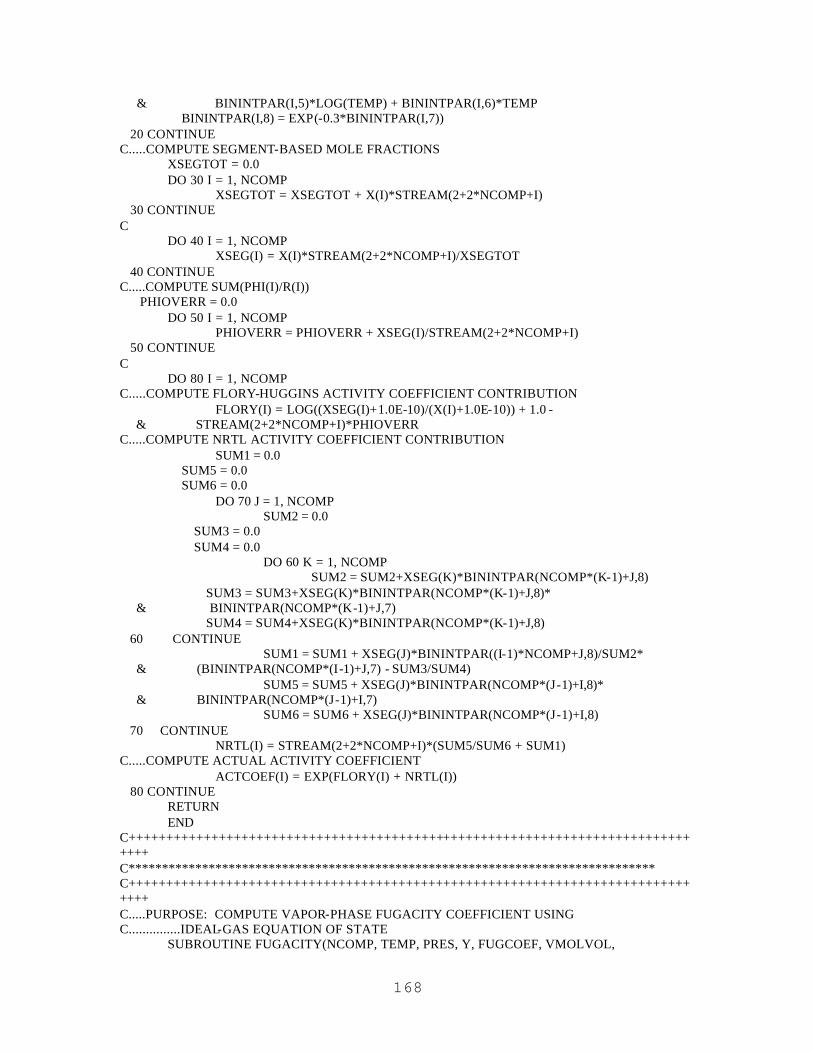
168
& BININTPAR(I,5)*LOG(TEMP) + BININTPAR(I,6)*TEMP BININTPAR(I,8) = EXP(-0.3*BININTPAR(I,7)) 20 CONTINUE C.....COMPUTE SEGMENT-BASED MOLE FRACTIONS XSEGTOT = 0.0 DO 30 I = 1, NCOMP XSEGTOT = XSEGTOT + X(I)*STREAM(2+2*NCOMP+I) 30 CONTINUE C DO 40 I = 1, NCOMP XSEG(I) = X(I)*STREAM(2+2*NCOMP+I)/XSEGTOT 40 CONTINUE C.....COMPUTE SUM(PHI(I)/R(I)) PHIOVERR = 0.0 DO 50 I = 1, NCOMP PHIOVERR = PHIOVERR + XSEG(I)/STREAM(2+2*NCOMP+I) 50 CONTINUE C DO 80 I = 1, NCOMP C.....COMPUTE FLORY-HUGGINS ACTIVITY COEFFICIENT CONTRIBUTION FLORY(I) = LOG((XSEG(I)+1.0E-10)/(X(I)+1.0E-10)) + 1.0 - & STREAM(2+2*NCOMP+I)*PHIOVERR C.....COMPUTE NRTL ACTIVITY COEFFICIENT CONTRIBUTION SUM1 = 0.0 SUM5 = 0.0 SUM6 = 0.0 DO 70 J = 1, NCOMP SUM2 = 0.0 SUM3 = 0.0 SUM4 = 0.0 DO 60 K = 1, NCOMP SUM2 = SUM2+XSEG(K)*BININTPAR(NCOMP*(K-1)+J,8) SUM3 = SUM3+XSEG(K)*BININTPAR(NCOMP*(K-1)+J,8)* & BININTPAR(NCOMP*(K-1)+J,7) SUM4 = SUM4+XSEG(K)*BININTPAR(NCOMP*(K-1)+J,8) 60 CONTINUE SUM1 = SUM1 + XSEG(J)*BININTPAR((I-1)*NCOMP+J,8)/SUM2* & (BININTPAR(NCOMP*(I-1)+J,7) - SUM3/SUM4) SUM5 = SUM5 + XSEG(J)*BININTPAR(NCOMP*(J-1)+I,8)* & BININTPAR(NCOMP*(J-1)+I,7) SUM6 = SUM6 + XSEG(J)*BININTPAR(NCOMP*(J-1)+I,8) 70 CONTINUE NRTL(I) = STREAM(2+2*NCOMP+I)*(SUM5/SUM6 + SUM1) C.....COMPUTE ACTUAL ACTIVITY COEFFICIENT ACTCOEF(I) = EXP(FLORY(I) + NRTL(I)) 80 CONTINUE RETURN END C+++++++++++++++++++++++++++++++++++++++++++++++++++++++++++++++++++++++++++++++ C******************************************************************************* C+++++++++++++++++++++++++++++++++++++++++++++++++++++++++++++++++++++++++++++++ C.....PURPOSE: COMPUTE VAPOR-PHASE FUGACITY COEFFICIENT USING C...............IDEAL-GAS EQUATION OF STATE SUBROUTINE FUGACITY(NCOMP, TEMP, PRES, Y, FUGCOEF, VMOLVOL,

169
& ENTHALPY) INTEGER NCOMP, I, ITMAX, IT REAL TEMP, PRES, Y(NCOMP), FUGCOEF(NCOMP), VMOLVOL, ENTHALPY REAL CRIT(NCOMP, 3), AM, BM, A(NCOMP), B(NCOMP), RIDEAL REAL F, DFDV, TOL PARAMETER (RIDEAL = 8.314, ITMAX = 1000, TOL = 1.0) C VMOLVOL = RIDEAL*TEMP/PRES FUGCOEF = 1.0 ENTHALPY = 0.0 C RETURN END C+++++++++++++++++++++++++++++++++++++++++++++++++++++++++++++++++++++++++++++++ C******************************************************************************* C+++++++++++++++++++++++++++++++++++++++++++++++++++++++++++++++++++++++++++++++ C.....PURPOSE: THIS SUBROUTINE COMPUTES THE VAPOR ENTHALPY C...............USING THE IDEAL GAS AT 298 K AS THE REFERENCE STATE C...............(POLYMER CONTRIBUTION IS IGNORED) SUBROUTINE VAPORENTHALPY(NCOMP, VAPOR, Y, VAPENTH) INTEGER NCOMP, I REAL VAPOR(3*NCOMP+4), Y(NCOMP), VAPENTH, TEMP, PRES REAL IGFORM(NCOMP), IGHTCAP(NCOMP, 5), HVAP(NCOMP, 4) REAL HPOLY(3), PSAT(NCOMP), FUGCOEF(NCOMP), VMOLVOL, ENTHALPY REAL EN(NCOMP) EXTERNAL ENTHPARAM, VAPORPRESSURE, FUGACITY C.....READ TEMPERATURE AND PRESSURE TEMP = VAPOR(1) PRES = VAPOR(2) C.....READ ENTHALPY PARAMETERS CALL ENTHPARAM(NCOMP, IGFORM, IGHTCAP, HVAP, HPOLY) C.....COMPUTE VAPOR PRESSURES CALL VAPORPRESSURE(NCOMP, TEMP, PSAT) C.....COMPUTE PURE COMPONENT ENTHALPIES EN = 0.0 DO 10 I = 1, NCOMP IF(VAPOR(2+2*NCOMP+I).EQ.1.0) THEN EN(I) = IGFORM(I) + & (IGHTCAP(I,1)*TEMP + IGHTCAP(I,2)*IGHTCAP(I,3)* & COSH(IGHTCAP(I,3)/TEMP)/SINH(IGHTCAP(I,3)/TEMP) - & IGHTCAP(I,4)*IGHTCAP(I,5)* & SINH(IGHTCAP(I,5)/TEMP)/COSH(IGHTCAP(I,5)/TEMP)) - & (IGHTCAP(I,1)*298.0 + IGHTCAP(I,2)*IGHTCAP(I,3)* & COSH(IGHTCAP(I,3)/298.0)/SINH(IGHTCAP(I,3)/298.0) - & IGHTCAP(I,4)*IGHTCAP(I,5)* & SINH(IGHTCAP(I,5)/298.0)/COSH(IGHTCAP(I,5)/298.0)) EN(I) = EN(I)/1000.0 END IF 10 CONTINUE C VAPENTH = 0.0 DO 20 I = 1, NCOMP VAPENTH = VAPENTH + Y(I)*EN(I) 20 CONTINUE

170
C.....COMPUTE VAPOR-PHASE ENTHALPY DEPARTURE FROM IDEALITY CALL FUGACITY(NCOMP, TEMP, PRES, Y, FUGCOEF, VMOLVOL, & ENTHALPY) VAPENTH = VAPENTH + ENTHALPY C RETURN END C+++++++++++++++++++++++++++++++++++++++++++++++++++++++++++++++++++++++++++++++ C******************************************************************************* C+++++++++++++++++++++++++++++++++++++++++++++++++++++++++++++++++++++++++++++++ C.....PURPOSE: THIS SUBROUTINE COMPUTES THE LIQUID STREAM ENTHALPY C...............USING IDEAL GAS AT 298 K AS REFERENCE STATE FOR SIMPLE SPECIES C...............AND AMORPHOUS POLYMER AT 313 K AS REFERENCE STATE FOR POLYMERS C...............(HEAT CAPACITY OF POLYMER FROM GAUR ET AL.) SUBROUTINE LIQUIDENTHALPY(NCOMP, LIQUID, X, LIQENTH) INTEGER NCOMPM U REAL LIQUID(3*NCOMP+4), LIQENTH, RIDEAL, HINT, X(NCOMP) REAL ACTCOEF(NCOMP), PSAT(NCOMP), TEMP REAL IGFORM(NCOMP), IGHTCAP(NCOMP, 5), HVAP(NCOMP, 4), HPOLY(3) REAL EN(NCOMP), DUMMYX(NCOMP), FUGCOEF(NCOMP), TR REAL ENTHALPY, CRIT(NCOMP, 3), VOL1, VOL2, PRES, ENTHALPYI REAL ACTTEMP2(NCOMP), ACTTEMP1(NCOMP), LMOLV(NCOMP) PARAMETER (RIDEAL = 8.314, HINT = 1.0) EXTERNAL ACTIVITY, VAPORPRESSURE, ENTHPARAM, FUGACITY EXTERNAL CRITICALPROPS C.....READ TEMPERATURE AND PRESSURE TEMP = LIQUID(1) PRES = LIQUID(2) C.....READ ENTHALPY PARAMETERS FOR COMPONENTS CALL ENTHPARAM(NCOMP, IGFORM, IGHTCAP, HVAP, HPOLY) C.....COMPUTE VAPOR PRESSURE CALL VAPORPRESSURE(NCOMP, TEMP, PSAT) C.....READ CRITICAL PROPERTIES CALL CRITICALPROPS(NCOMP, CRIT) C.....COMPUTE PURE COMPONENT ENTHALPY EN = 0.0 DO 10 I = 1, NCOMP IF(LIQUID(2+2*NCOMP+I).EQ.1.0) THEN C.....COMPUTE PURE COMPONENT ENTHALPY (IDEAL GAS HEAT OF FORMATION C......................................AND IDEAL GAS HEAT CAPACITY PART) EN(I) = IGFORM(I) + & (IGHTCAP(I,1)*TEMP + IGHTCAP(I,2)*IGHTCAP(I,3)* & COSH(IGHTCAP(I,3)/TEMP)/SINH(IGHTCAP(I,3)/TEMP) - & IGHTCAP(I,4)*IGHTCAP(I,5)* & SINH(IGHTCAP(I,5)/TEMP)/COSH(IGHTCAP(I,5)/TEMP)) - & (IGHTCAP(I,1)*298.0 + IGHTCAP(I,2)*IGHTCAP(I,3)* & COSH(IGHTCAP(I,3)/298.0)/SINH(IGHTCAP(I,3)/298.0) - & IGHTCAP(I,4)*IGHTCAP(I,5)* & SINH(IGHTCAP(I,5)/298.0)/COSH(IGHTCAP(I,5)/298.0)) DUMMYX = 0.0 DUMMYX(I) = 1.0 C.....COMPUTE PURE COMPONENT ENTHALPY (RAISE IDEAL GAS FROM ZERO PRESSURE C......................................TO SATURATION PRESSURE) CALL FUGACITY(NCOMP, TEMP, PSAT(I), DUMMYX, FUGCOEF, VMOLVOL,

171
& ENTHALPY) EN(I) = EN(I) + ENTHALPY TR = TEMP/CRIT(I,1) C.....COMPUTE PURE COMPONENT ENTHALPY (CONDENSE IDEAL GAS AT SATURATION C......................................CONDITIONS) EN(I) = EN(I) - (HVAP(I,1)*(1.0 - TR)** & (HVAP(I,2) + HVAP(I,3)*TR + HVAP(I,4)*TR**2.0)) LIQUID(1) = LIQUID(1) + HINT CALL LIQUIDMOLARVOLUME(NCOMP, LIQUID, LMOLV) LIQUID(1) = LIQUID(1) - HINT VOL2 = LMOLV(I) LIQUID(1) = LIQUID(1) - HINT CALL LIQUIDMOLARVOLUME(NCOMP, LIQUID, LMOLV) LIQUID(1) = LIQUID(1) + HINT VOL1 = LMOLV(I) CALL LIQUIDMOLARVOLUME(NCOMP, LIQUID, LMOLV) C.....COMPUTE PURE COMPONENT ENTHALPY (BRING LIQUID TO SYSTEM PRESSURE) EN(I) = EN(I) + (LMOLV(I) - TEMP* & ((VOL2 - VOL1)/(2.0*HINT)))*(PRES - PSAT(I)) C.....CONVERT J/KMOL TO J/MOL EN(I) = EN(I) / 1000.0 ELSE C.....PURE COMPONENT LIQUID ENTHALPY FOR POLYMER EN(I) = LIQUID(2+2*NCOMP+I)* & (HPOLY(1) + (HPOLY(2)/2.0*TEMP**2.0 + HPOLY(3)*TEMP) & - (HPOLY(2)/2.0*313.0**2.0 + HPOLY(3)*313.0)) END IF 10 CONTINUE C.....COMPUTE MIXTURE ENTHALPY WITHOUT EXCESS ENTHALPY OF MIXING EFFECTS ENTHALPYI = 0.0 DO 20 I = 1, NCOMP ENTHALPYI = ENTHALPYI + X(I)*EN(I) 20 CONTINUE C LIQUID(1) = LIQUID(1) + HINT CALL ACTIVITY(NCOMP, LIQUID, X, ACTCOEF) LIQUID(1) = LIQUID(1) - HINT ACTTEMP2 = ACTCOEF LIQUID(1) = LIQUID(1) - HINT CALL ACTIVITY(NCOMP, LIQUID, X, ACTCOEF) LIQUID(1) = LIQUID(1) + HINT ACTTEMP1 = ACTCOEF C LIQENTH = 0.0 DO 30 I = 1, NCOMP LIQENTH = LIQENTH + (LOG(ACTTEMP2(I))-LOG(ACTTEMP1(I)))/ & (2.0*HINT)*X(I) 30 CONTINUE C.....COMPUTE EXCESS ENTHALPY OF MIXING LIQENTH = LIQENTH*(-1.0)*(TEMP**2.0)*RIDEAL C LIQENTH = LIQENTH + ENTHALPYI C RETURN END

172
C+++++++++++++++++++++++++++++++++++++++++++++++++++++++++++++++++++++++++++++++ C******************************************************************************* C+++++++++++++++++++++++++++++++++++++++++++++++++++++++++++++++++++++++++++++++ C.....PURPOSE: THIS SUBROUTINE NORMALIZES MOLE FRACTIONS SUBROUTINE NORMALIZE(NCOMP, X) INTEGER NCOMP, I REAL X(NCOMP), TOT C TOT = 0.0 DO 10 I = 1, NCOMP TOT = TOT + X(I) 10 CONTINUE C DO 20 I = 1, NCOMP X(I) = X(I)/TOT 20 CONTINUE C RETURN END C+++++++++++++++++++++++++++++++++++++++++++++++++++++++++++++++++++++++++++++++ C******************************************************************************* C+++++++++++++++++++++++++++++++++++++++++++++++++++++++++++++++++++++++++++++++ C.....PURPOSE: THIS SUBROUTINE TAKES A STREAM WITH MASS FLOW RATES AND FILLS C...............IN THE APPROPRIATE MOLE FLOW RATES SUBROUTINE MASSTOMOLE(NCOMP, STREAM) INTEGER NCOMP, I REAL STREAM(3*NCOMP+4), MW(NCOMP) EXTERNAL MOLECULARWEIGHT C CALL MOLECULARWEIGHT(NCOMP, MW) C DO 10 I = 1, NCOMP STREAM(NCOMP+2+I) = STREAM(2+I)/(MW(I)*STREAM(2*NCOMP+2+I)) 10 CONTINUE C RETURN END C+++++++++++++++++++++++++++++++++++++++++++++++++++++++++++++++++++++++++++++++ C******************************************************************************* C+++++++++++++++++++++++++++++++++++++++++++++++++++++++++++++++++++++++++++++++ C.....PURPOSE: THIS SUBROUTINE TAKES A STREAM WITH MOLE FLOW RATES AND FILLS C...............IN THE APPROPRIATE MASS FLOW RATES SUBROUTINE MOLETOMASS(NCOMP, STREAM) INTEGER NCOMP, I REAL STREAM(3*NCOMP+4), MW(NCOMP) EXTERNAL MOLECULARWEIGHT C CALL MOLECULARWEIGHT(NCOMP, MW) C DO 10 I = 1, NCOMP

173
STREAM(2+I) = STREAM(NCOMP+2+I)*MW(I)*STREAM(2*NCOMP+2+I) 10 CONTINUE C RETURN END C$$$$$$$$$$$$$$$$$$$$$$$$$$$$$$$$$$$$$$$$$$$$$$$$$$$$$$$$$$$$$$$$$$$$$$$$$$$$$$$ C******************************************************************************* C$$$$$$$$$$$$$$$$$$$$$$$$$$$$$$$$$$$$$$$$$$$$$$$$$$$$$$$$$$$$$$$$$$$$$$$$$$$$$$$ C*****PHYSICAL PROPERTY PARAMETERS BELOW**************************************** C$$$$$$$$$$$$$$$$$$$$$$$$$$$$$$$$$$$$$$$$$$$$$$$$$$$$$$$$$$$$$$$$$$$$$$$$$$$$$$$ C******************************************************************************* C$$$$$$$$$$$$$$$$$$$$$$$$$$$$$$$$$$$$$$$$$$$$$$$$$$$$$$$$$$$$$$$$$$$$$$$$$$$$$$$ SUBROUTINE MOLECULARWEIGHT(NCOMP, MW) INTEGER NCOMP REAL MW(NCOMP) C.....MOLECULAR WEIGHT = KG/MOL-SEG MW(1) = 18.0152/1000.0 MW(2) = 113.159/1000.0 MW(3) = 226.318/1000.0 MW(4) = 131.1742/1000.0 MW(5) = 60.0524/1000.0 MW(6) = 99.1754/1000.0 MW(7) = 113.159/1000.0 C RETURN END C******************************************************************************* SUBROUTINE ANTOINE(NCOMP, ANTCOEF) C.....DAUBERT, T. E., AND R. P. DANNER C.....PHYSICAL AND THERMODYNAMIC PROPERTIES OF PURE CHEMICALS VOLUME 3 INTEGER NCOMP REAL ANTCOEF(NCOMP, 5) C.....VAPOR PRESSURE (PA), TEMPERATURE (K) ANTCOEF(1,1) = 7.3649E+01 ANTCOEF(1,2) = -7.2582E+03 ANTCOEF(1,3) = -7.3037E+00 ANTCOEF(1,4) = 4.1653E-06 ANTCOEF(1,5) = 2.0000E+00 C * ANTCOEF(2,1) = 7.4172E+01 ANTCOEF(2,2) = -1.0469E+04 ANTCOEF(2,3) = -6.8944E+00 ANTCOEF(2,4) = 1.2113E-18 ANTCOEF(2,5) = 6.0000E+00 C * ANTCOEF(3,1) = -40.0 ANTCOEF(3,2) = 0.0 ANTCOEF(3,3) = 0.0 ANTCOEF(3,4) = 0.0 ANTCOEF(3,5) = 0.0 C * ANTCOEF(4,1) = -40.0 ANTCOEF(4,2) = 0.0 ANTCOEF(4,3) = 0.0 ANTCOEF(4,4) = 0.0
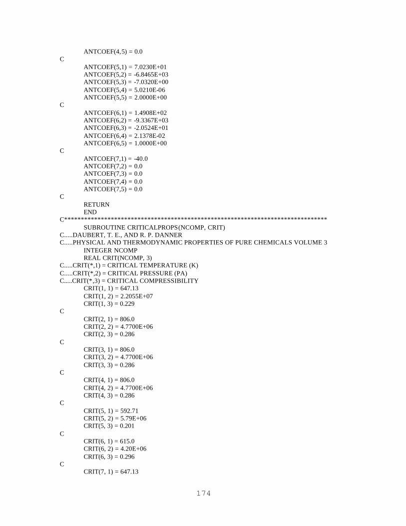
174
ANTCOEF(4,5) = 0.0 C ANTCOEF(5,1) = 7.0230E+01 ANTCOEF(5,2) = -6.8465E+03 ANTCOEF(5,3) = -7.0320E+00 ANTCOEF(5,4) = 5.0210E-06 ANTCOEF(5,5) = 2.0000E+00 C ANTCOEF(6,1) = 1.4908E+02 ANTCOEF(6,2) = -9.3367E+03 ANTCOEF(6,3) = -2.0524E+01 ANTCOEF(6,4) = 2.1378E-02 ANTCOEF(6,5) = 1.0000E+00 C ANTCOEF(7,1) = -40.0 ANTCOEF(7,2) = 0.0 ANTCOEF(7,3) = 0.0 ANTCOEF(7,4) = 0.0 ANTCOEF(7,5) = 0.0 C RETURN END C******************************************************************************* SUBROUTINE CRITICALPROPS(NCOMP, CRIT) C.....DAUBERT, T. E., AND R. P. DANNER C.....PHYSICAL AND THERMODYNAMIC PROPERTIES OF PURE CHEMICALS VOLUME 3 INTEGER NCOMP REAL CRIT(NCOMP, 3) C.....CRIT(*,1) = CRITICAL TEMPERATURE (K) C.....CRIT(*,2) = CRITICAL PRESSURE (PA) C.....CRIT(*,3) = CRITICAL COMPRESSIBILITY CRIT(1, 1) = 647.13 CRIT(1, 2) = 2.2055E+07 CRIT(1, 3) = 0.229 C CRIT(2, 1) = 806.0 CRIT(2, 2) = 4.7700E+06 CRIT(2, 3) = 0.286 C CRIT(3, 1) = 806.0 CRIT(3, 2) = 4.7700E+06 CRIT(3, 3) = 0.286 C CRIT(4, 1) = 806.0 CRIT(4, 2) = 4.7700E+06 CRIT(4, 3) = 0.286 C CRIT(5, 1) = 592.71 CRIT(5, 2) = 5.79E+06 CRIT(5, 3) = 0.201 C CRIT(6, 1) = 615.0 CRIT(6, 2) = 4.20E+06 CRIT(6, 3) = 0.296 C CRIT(7, 1) = 647.13

175
CRIT(7, 2) = 2.2055E+07 CRIT(7, 3) = 0.229 C RETURN END C******************************************************************************* SUBROUTINE MOLVOLP(NCOMP, MOLV) C.....DIPPR LIQUID MOLAR VOLUME PARAMETERS FOR SIMPLE SPECIES C.....TAIT EQUATION PARAMETERS FOR NYLON-6 (DATA FROM ZOLLER) INTEGER NCOMP REAL MOLV(NCOMP, 5) C.....FOR SIMPLE SPECIES, SEE BELOW C.....MOLV(I,1) = DIPPR A LIQUID MOLAR VOLUME PARAMETER (MOL/M^3) C.....MOLV(I,2) = DIPPR B LIQUID MOLAR VOLUME PARAMETER C.....MOLV(I,3) = DIPPR C LIQUID MOLAR VOLUME PARAMETER (K) C.....MOLV(I,4) = DIPPR D LIQUID MOLAR VOLUME PARAMETER MOLV(1,1) = 5.4590E+00 * 1000.0 MOLV(1,2) = 3.0542E-01 MOLV(1,3) = 6.4713E+02 MOLV(1,4) = 8.1000E-02 C MOLV(2,1) = 7.1180E-01 * 1000.0 MOLV(2,2) = 2.5400E-01 MOLV(2,3) = 8.0600E+02 MOLV(2,4) = 2.8570E-01 C MOLV(3,1) = 7.1180E-01 * 1000.0 MOLV(3,2) = 2.5400E-01 MOLV(3,3) = 8.0600E+02 MOLV(3,4) = 2.8570E-01 C MOLV(4,1) = 7.1180E-01 * 1000.0 MOLV(4,2) = 2.5400E-01 MOLV(4,3) = 8.0600E+02 MOLV(4,4) = 2.8570E-01 C MOLV(5,1) = 1.5791E+00 * 1000.0 MOLV(5,2) = 2.6954E-01 MOLV(5,3) = 5.9271E+02 MOLV(5,4) = 2.6843E-01 C MOLV(6,1) = 7.0886E-01 * 1000.0 MOLV(6,2) = 2.5517E-01 MOLV(6,3) = 6.1500E+02 MOLV(6,4) = 2.7070E-01 C.....FOR POLYMER, SEE BELOW C.....MOLV(I,1) = TAIT AZERO (M^3/KG) C.....MOLV(I,2) = TAIT AONE (M^3/KG C) C.....MOLV(I,3) = TAIT ZTWO (M^3/KG C^2) C.....MOLV(I,4) = TAIT BZERO (PA) C.....MOLV(I,5) = TAIT BONE (1/C) MOLV(7,1) = 9.4650E-4 MOLV(7,2) = 0.0000E+00 MOLV(7,3) = 1.2273E-09 MOLV(7,4) = 3.3232E+08 MOLV(7,5) = 3.8193E-03

176
C RETURN END C******************************************************************************* SUBROUTINE BINARY(NCOMP, BININTPAR) INTEGER NCOMP REAL BININTPAR(NCOMP*NCOMP, 8) C BININTPAR = 0.0 C C.....THIS IS THE MATRIX SET-UP THAT STORES POLYNRTL BINARY PARAMETERS C.....USER INPUT IS A-D FOR EACH BINARY INTERACTION C.....TAU = A + B/TEMP(K) + C*LN(TEMP) + D*TEMP C.....G = EXP(-0.3*TAU) C.....A-D FOR LIKE INTERACTIONS (I-I) IS ALWAYS ZERO C.....PARAM SET -UP C..........FIRST COLUMN IS COMPONENT I C..........SECOND COLUMN IS COMPONENT J C..........THIRD-SIXTH COLUMN IS BINARY INTERACTION PARAMETER FOR I-J PAIR C..........SEVENTH COLUMN IS COMPUTED TAU FOR I-J C..........EIGTH COLUMN IS COMPUTED G FOR I-J C.....I J A B C D TAU G C.....1 1 0.0 0.0 0.0 0.0 0.0 1.0 C.....1 2 0.0 0.0 0.0 0.0 0.0 1.0 C.....1 . 0.0 0.0 0.0 0.0 0.0 1.0 C.....1 n 0.0 0.0 0.0 0.0 0.0 1.0 C.....2 1 0.0 0.0 0.0 0.0 0.0 1.0 C.....2 2 0.0 0.0 0.0 0.0 0.0 1.0 C.....2 . 0.0 0.0 0.0 0.0 0.0 1.0 C.....2 n 0.0 0.0 0.0 0.0 0.0 1.0 C.....3 1 0.0 0.0 0.0 0.0 0.0 1.0 C...... . 0.0 0.0 0.0 0.0 0.0 1.0 C.....n n 0.0 0.0 0.0 0.0 0.0 1.0 BININTPAR(2,3) = -0.313 BININTPAR(2,4) = -15.4 BININTPAR(2,5) = 0.0495 BININTPAR(2,6) = 0.0 C BININTPAR(8,3) = 0.628 BININTPAR(8,4) = -13.7 BININTPAR(8,5) = -0.0898 BININTPAR(8,6) = 0.0 C RETURN END C******************************************************************************* SUBROUTINE ENTHPARAM(NCOMP, IGFORM, IGHTCAP, HVAP, HPOLY) INTEGER NCOMP REAL IGFORM(NCOMP), IGHTCAP(NCOMP,5), HVAP(NCOMP,4), HPOLY(3) C C.....DAUBERT, T. E., AND R. P. DANNER C.....PHYSICAL AND THERMODYNAMIC PROPERTIES OF PURE CHEMICALS VOLUME 3 C C.....VAN KREVELEN, D. W. C.....PROPERTIES OF POLYMERS, 3RD ED., PAGES 112, 123 (1990) C
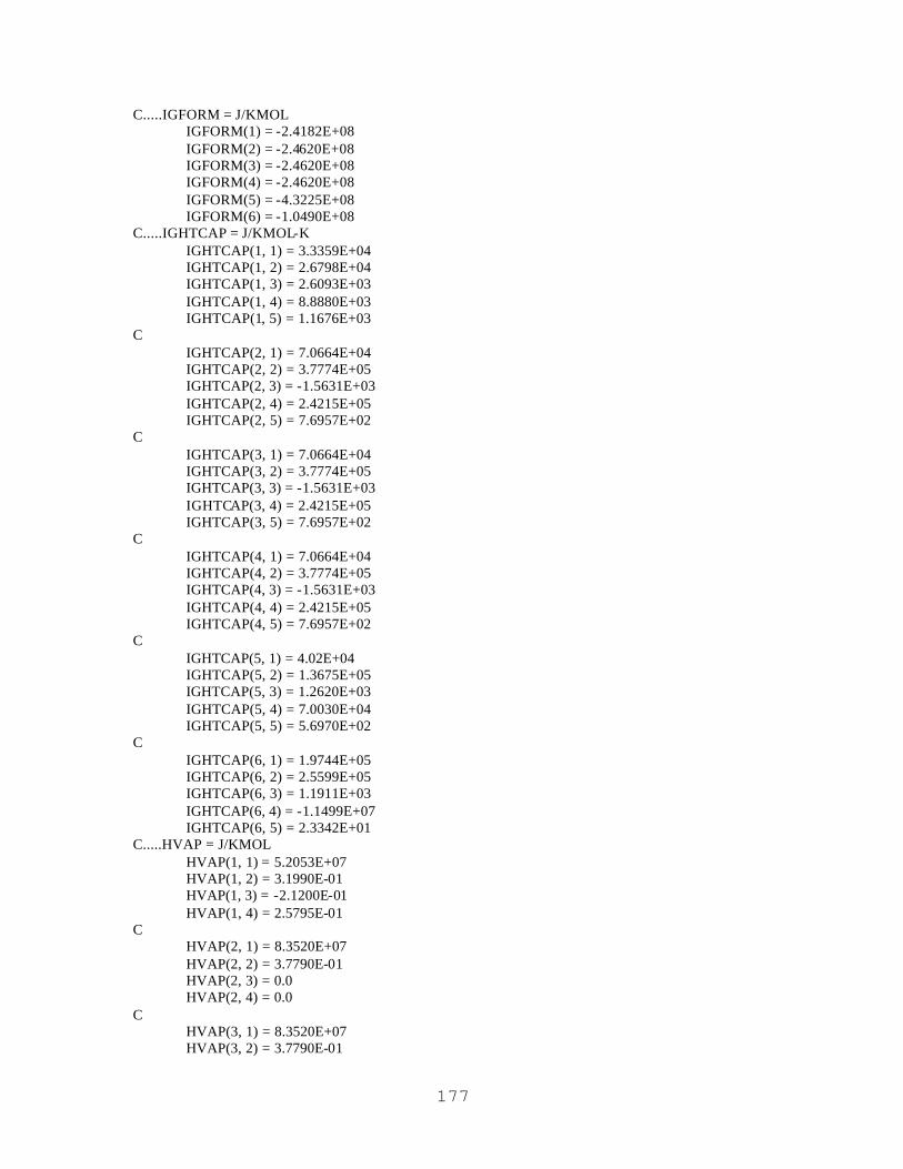
177
C.....IGFORM = J/KMOL IGFORM(1) = -2.4182E+08 IGFORM(2) = -2.4620E+08 IGFORM(3) = -2.4620E+08 IGFORM(4) = -2.4620E+08 IGFORM(5) = -4.3225E+08 IGFORM(6) = -1.0490E+08 C.....IGHTCAP = J/KMOL-K IGHTCAP(1, 1) = 3.3359E+04 IGHTCAP(1, 2) = 2.6798E+04 IGHTCAP(1, 3) = 2.6093E+03 IGHTCAP(1, 4) = 8.8880E+03 IGHTCAP(1, 5) = 1.1676E+03 C IGHTCAP(2, 1) = 7.0664E+04 IGHTCAP(2, 2) = 3.7774E+05 IGHTCAP(2, 3) = -1.5631E+03 IGHTCAP(2, 4) = 2.4215E+05 IGHTCAP(2, 5) = 7.6957E+02 C IGHTCAP(3, 1) = 7.0664E+04 IGHTCAP(3, 2) = 3.7774E+05 IGHTCAP(3, 3) = -1.5631E+03 IGHTCAP(3, 4) = 2.4215E+05 IGHTCAP(3, 5) = 7.6957E+02 C IGHTCAP(4, 1) = 7.0664E+04 IGHTCAP(4, 2) = 3.7774E+05 IGHTCAP(4, 3) = -1.5631E+03 IGHTCAP(4, 4) = 2.4215E+05 IGHTCAP(4, 5) = 7.6957E+02 C IGHTCAP(5, 1) = 4.02E+04 IGHTCAP(5, 2) = 1.3675E+05 IGHTCAP(5, 3) = 1.2620E+03 IGHTCAP(5, 4) = 7.0030E+04 IGHTCAP(5, 5) = 5.6970E+02 C IGHTCAP(6, 1) = 1.9744E+05 IGHTCAP(6, 2) = 2.5599E+05 IGHTCAP(6, 3) = 1.1911E+03 IGHTCAP(6, 4) = -1.1499E+07 IGHTCAP(6, 5) = 2.3342E+01 C.....HVAP = J/KMOL HVAP(1, 1) = 5.2053E+07 HVAP(1, 2) = 3.1990E-01 HVAP(1, 3) = -2.1200E-01 HVAP(1, 4) = 2.5795E-01 C HVAP(2, 1) = 8.3520E+07 HVAP(2, 2) = 3.7790E-01 HVAP(2, 3) = 0.0 HVAP(2, 4) = 0.0 C HVAP(3, 1) = 8.3520E+07 HVAP(3, 2) = 3.7790E-01

178
HVAP(3, 3) = 0.0 HVAP(3, 4) = 0.0 C HVAP(4, 1) = 8.3520E+07 HVAP(4, 2) = 3.7790E-01 HVAP(4, 3) = 0.0 HVAP(4, 4) = 0.0 C HVAP(5, 1) = 1.26E+07 HVAP(5, 2) = -1.11 HVAP(5, 3) = 6.30E-02 HVAP(5, 4) = 1.142 C HVAP(6, 1) = 5.7160E+07 HVAP(6, 2) = 0.42100 HVAP(6, 3) = 0.0 HVAP(6, 4) = 0.0 C.....HPOLY(1) = REFERENCE ENTHALPY AT 313 K (J/MOL-SEG) C.....HPOLY(2) = CP CONSTANT ONE (J/MOL-SEG K^2) C.....HPOLY(3) = CP CONSTANT TWO (J/MOL-SEG K) HPOLY(1) = -3.24E5 HPOLY(2) = 0.153 HPOLY(3) = 223.95 C RETURN END

179
5 A Model for the Diffusivity of Water and Caprolactam
in Concentrated Nylon-6 Solutions114
In Chapters 2 through 4, we developed the reaction set and physical property system for
nylon-6 polymerizations. In this chapter, we shift gears and tackle an active area of
research in the field of step-growth polymerizations – that is, the area of mass-transfer
limited polymerization. The first step in mass-transfer analysis is to quantify the
molecular diffusion coefficients of volatile species. This chapter presents a model for the
molecular diffusion coefficient of water and caprolactam in concentrated nylon-6
solutions at typical polymerization conditions. The model is based on the Vrentas-
Duda115 free-volume theory for diffusion coefficients and utilizes the experimental data
of Nagasubramanian and Reimschuessel116. The model estimates the effects of
concentration and temperature on the diffusion coefficients.
Chapter organization is below:
• 5.1 – Introduction to the problem of diffusion in concentrated nylon-6 solutions
• 5.2 – Simulation problem description
• 5.3 – Overview of theory of reaction/diffusion
• 5.4 – Details on implementation of theory
• 5.5 – Results and discussion
• 5.6 – Application of the new models for diffusivities
• 5.7 – Conclusions
114 Adapted from a document coauthored by Tom Lee and Y. A. Liu 115 Vrentas, J. S., and J. L. Duda, “Diffusion in Polymer-Solvent Systems. I. Reexamination of the Free-
Volume Theory,” Journal of Polymer Science, Polymer Physics Edition, 15, pp. 403-416 (1977). 116 Nagasubramanian, K., and H. K. Reimschuessel, “Diffusion of Water and Caprolactam in Nylon-6
Melts,” Journal of Applied Polymer Science, 17, pp. 1663-1677 (1973).

180
5.1 Introduction
It is well known that the finishing stages of step-growth polymer synthesis are mass-
transfer limited, rather than kinetically limited. There are three typical approaches to
finishing operations for producing nylon-6. The first approach involves inert gas
injection117 into the concentrated polymer solution to remove water, thus driving reaction
equilibrium towards high-molecular-weight polymer. We then pelletize the polymer and
perform hot-water extraction followed by drying in order to remove residual monomer
and oligomers. The second approach for finishing a nylon-6 solution involves vacuum-
devolatization118 of the concentrated high-molecular-weight solution, thus removing
residual monomer and water at the same time. This produces a melt that can be directly
used for spinning fibers, thus avoiding pelletizing, hot-water extraction, and drying. A
third approach for finishing polymers is solid-state polymerization. 119 Solid-state
polymerization takes place at lower temperatures than the melt process, and essentially
consists of passing a current of inert gas over polymer pellets or by applying vacuum to
remove volatile reaction byproducts, including water, thus driving reaction equilibrium to
create a very high molecular weight product.
All of these finishing steps are similar in that they involve simultaneous reaction and
mass transfer. The polymer solutions are no longer in thermodynamic equilibrium with
their surroundings. When we dig under the idiosyncrasies of each process, such as
mixing effects, interfacial area generation, boiling, and crystallization, we find the same
basic core for understanding these processes. The common starting point in analysis is
developing a quantitative model to predict the diffusion coefficient of volatile species
117 Russell, W. N., A. H. Wiesner, and O. E. Snider, “Continuous Polymerization of ε-Caprolactam,”
United States Patent #3,294,756 (1966). 118 Yates, S. L., C. J. Cole, A. H. Wiesner, and J. W. Wagner, “Two-Stage Hydrolysis Process for the
Preparation of Nylon-6,” United States Patent #4,310,659 (1982). 119 Kang, C. K., “Modeling of Solid-State Polymerization of Poly(ethylene terephthalate),” Journal of
Applied Polymer Science, 68, pp. 837-846 (1998).
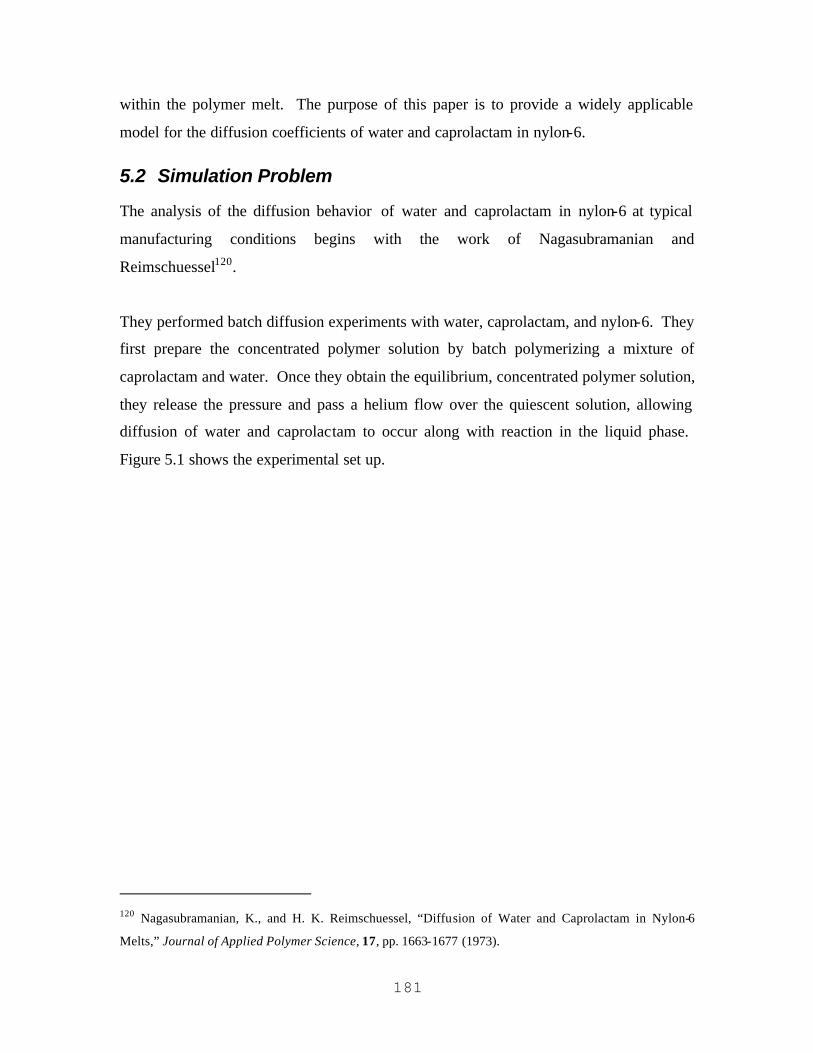
181
within the polymer melt. The purpose of this paper is to provide a widely applicable
model for the diffusion coefficients of water and caprolactam in nylon-6.
5.2 Simulation Problem
The analysis of the diffusion behavior of water and caprolactam in nylon-6 at typical
manufacturing conditions begins with the work of Nagasubramanian and
Reimschuessel120.
They performed batch diffusion experiments with water, caprolactam, and nylon-6. They
first prepare the concentrated polymer solution by batch polymerizing a mixture of
caprolactam and water. Once they obtain the equilibrium, concentrated polymer solution,
they release the pressure and pass a helium flow over the quiescent solution, allowing
diffusion of water and caprolactam to occur along with reaction in the liquid phase.
Figure 5.1 shows the experimental set up.
120 Nagasubramanian, K., and H. K. Reimschuessel, “Diffusion of Water and Caprolactam in Nylon-6
Melts,” Journal of Applied Polymer Science, 17, pp. 1663-1677 (1973).
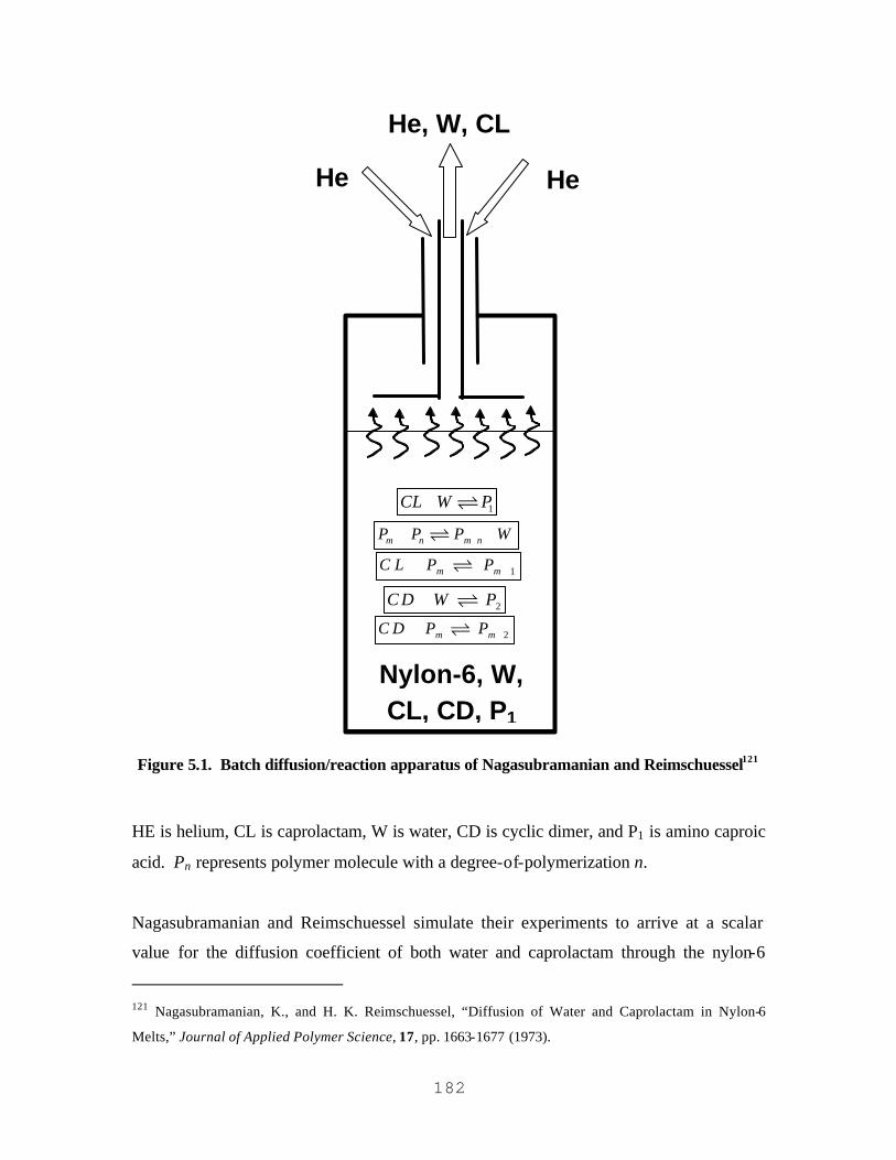
182
HeHe
He, W, CL
Nylon-6, W, CL, CD, P1
1CL W P+ �m n m nP P P W++ +�
1m mC L P P ++ �
2C D W P+ �2m mC D P P ++ �
Figure 5.1. Batch diffusion/reaction apparatus of Nagasubramanian and Reimschuessel121
HE is helium, CL is caprolactam, W is water, CD is cyclic dimer, and P1 is amino caproic
acid. Pn represents polymer molecule with a degree-of-polymerization n.
Nagasubramanian and Reimschuessel simulate their experiments to arrive at a scalar
value for the diffusion coefficient of both water and caprolactam through the nylon-6
121 Nagasubramanian, K., and H. K. Reimschuessel, “Diffusion of Water and Caprolactam in Nylon-6
Melts,” Journal of Applied Polymer Science, 17, pp. 1663-1677 (1973).
183
melt. Strictly speaking, these diffusion coefficients pertain only to concentrated solutions
in the 10% by weight caprolactam range and at 265 °C, since these are the conditions
under which data was generated. They use Higbie122 penetration theory along with the
reaction kinetics scheme of Reimschuessel and Nagasubramanian123.
While this may suffice for making rough mass-transfer rate calculations for processes that
mirror the conditions used in their study, questions arise on how to apply their results in
differing situations. For example, we may ask, what happens to the diffusion coefficient
if a finishing reactor is run at 245 °C? Another question would be how to apply these
results to analyzing solid-state polymerization, where the concentration of reaction by-
products is far lower than that found in the batch polymerization experiment.
Additionally, more recent developments concerning our growing understanding of nylon-
6 polymerizations further cloud our ability to judge the applicability of their results even
to reaction conditions similar to theirs. One such complication is that they use a now-
outdated reaction kinetics scheme for their analysis - modern analyses of nylon-6
polymerizations use the newer kinetic scheme of Arai et al.124
We know that in general, the diffusion coefficient in polymer solutions is a strong
function of concentration125. In addition, we know that temperature influences the
diffusion coefficient. In order to estimate these dependencies on temperature and
concentration, we need the diffusion coefficient as a function of temperature and
concentration, rather than just a scalar value. This will allow us to at least estimate the
change in the diffusion coefficient with temperature and volatile concentration, rather
122 Higbie, R., “The Rate of Absorption of a Pure Gas Into a Liquid Still During Short Periods of
Exposure,” Transactions of the Americal Institute of Chemical Engineers, 31, pp. 365-389 (1935). 123 Reimschuessel, H. K., and K. Nagasubramanian, “Optimization of Caprolactam Polymerization,”
Chemical Engineering Science , 27, pp. 1119-1130 (1972). 124 Arai, Y., K. Tai, H. Teranishi, and T. Tagawa, “Kinetics of Hydrolytic Polymerization of ε-
Caprolactam: 3. Formation of Cyclic Dimer,” Polymer, 22, pp. 273-277 (1981). 125 Vrentas, J. S., and J. L. Duda, “Diffusion in Polymer-Solvent Systems. I. Reexamination of the Free-
Volume Theory,” Journal of Polymer Science, Polymer Physics Edition, 15, pp. 403-416 (1977).
184
than remain paralyzed by questions regarding how exactly to apply Nagasubramanian
and Reimschuessel’s results to the engineering analysis of differing polymer finishing
techniques.
In addition to a more generally applicable function to represent the diffusion coefficient,
we also wish to predict the interfacial liquid concentration of volatile and non-volatile
species. Nagasubramanian and Reimschuessel did not predict these quantities during
their analysis. They assume a constant interfacial concentration, which may not be valid,
and extrapolate the interfacial concentration of caprolactam from the experimental data –
this is not possible in the general analysis of industrial finishing reactors. In addition,
they regress the interfacial concentration of water as a parameter. One generally wishes
to predict this value in order to minimize the amount of free parameters that must be
estimated from plant data.
Specifically, our goal is to provide a method for estimating the concentration/temperature
dependence of the diffusion coefficients of water and caprolactam in concentrated nylon-
6 solutions. Our intended audience consists of users of advanced polymerization
simulation tools. Our results are useful for the quantitative modeling of industrial nylon-
6 polymerization processes.
5.3 Theoretical
5.3.1 Mass-Transfer Theory
We use penetration theory126 to analyze this diffusion/reaction problem. The penetration
theory can successfully describe a wide range of complicated, industrial nylon-6
126 Higbie, R., “The Rate of Absorption of a Pure Gas Into a Liquid Still During Short Periods of
Exposure,” Transactions of the Americal Institute of Chemical Engineers, 31, pp. 365-389 (1935).

185
processes as demonstrated by Laubriet et al.127 and is also the industrial standard for
simulating the mass-transfer aspects of polymerization processes.
Figure 5.2 shows the penetration-theory representation of the concentration gradient in
the liquid phase:
Co
nce
ntr
atio
n
Liquid Phase
VaporPhase
,i LC
, *i LC
Figure 5.2. Penetration theory representation of the concentration gradient in the diffusion
of a species through the liquid phase into the vapor phase – CL is the bulk-phase
concentration while CL* is the liquid-phase interfacial concentration
The discontinuity between the concentrations is due to the equality of chemical potentials
rather than the equality of concentrations. We typically assume that the liquid phase at
the interface is in thermodynamic equilibrium with the vapor phase. Relative to the
liquid phase, we typically assume that no mass-transfer resistance is found in the vapor
phase. 127 Laubriet, C., B. LeCorre, and K. Y. Choi, “Two-Phase Model for Continuous Final Stage Melt
Polycondensation of Poly(ethylene terephthalate). 1. Steady-State Analysis,” Industrial and Engineering
Chemistry Research, 30, pp. 2-12 (1991).

186
We compute the evaporation rate for species i out of the liquid phase Ei as follows:
( ), , , *i L i i L i L LE k a C C V= − (5.1)
iE has units of mol/s. The mass-transfer coefficient for species i is ,L ik a , which has
units of s-1. ,i LC is the bulk liquid concentration of species i (mol/m3), while , *i LC is the
liquid interfacial concentration of i. Lastly, LV is the volume of the liquid phase (m3).
The term a of the mass-transfer coefficient is the specific surface area of the liquid phase
– the ratio of the interfacial surface area between the vapor and liquid phase, Aint (m2),
and the liquid phase volume LV . Therefore, we can cancel out these terms and write:
( ), int , , *i L i i L i LE k A C C= − (5.2)
where Aint is the actual interfacial area (m2).
According to penetration theory, we express ,L ik as twice the square root of the ratio of
the diffusion coefficient for species i, iD (m2/s), and the product of p and the contact time
tc.
( ),
,
,2 i i L
L ic
C Tk
tπ=
D (5.3)
We assume that the diffusion coefficient is a function of the bulk-phase composition and
temperature.
We compute the concentration at the interface by assuming that the liquid interface is in
thermodynamic equilibrium with the vapor phase. At low pressure/elevated temperature
187
and for a concentrated solution, we would expect that the ratio of the vapor-phase mole
fraction yi and the liquid-phase mole fraction xi would be equal to the saturation pressure
of species i to the system pressure P:
sat
i i
i
y Px P
= (5.4)
We cannot apply this method for predicting the liquid mole fraction of non-volatile
species, such as nylon-6. Their evaporation rate is zero and thus their vapor mole
fraction is zero. We therefore approximate the mole fraction of nylon-6 at the interface
by assuming that it makes up the balance:
NYLON W CL1x x x= − − (5.5)
In reality, a small but unknown portion of the balance contains amino caproic acid and
oligomers – for sake of simplicity, we will ignore this complication.
5.3.2 Modeling the Diffusivity of Volatile Species in Concentrated
Polymer Solutions
In a solution of polymer and small molecules, the diffusivity of volatiles iD depends on
the polymer concentration and temperature. The diffusivity is also a function of polymer
molecular weight but only at low polymer concentrations 128. We use Vrentas-Duda free-
volume theory129 to characterize the diffusivity of caprolactam and water through molten
nylon-6. Free-volume models have been successfully used to describe diffusion
128 Vrentas, J. S., and C. H. Chu, “Molecular Weight Dependence of the Diffusion Coefficient for the
Polystyrene-Toluene System,” Journal of Polymer Science. Part B. Polymer Physics, 27, pp. 465-468
(1989). 129 Vrentas, J. S., and J. L. Duda, “Diffusion in Polymer-Solvent Systems. I. Reexamination of the Free-
Volume Theory,” Journal of Polymer Science, Polymer Physics Edition, 15, pp. 403-416 (1977).
188
coefficients for many industrial processes, including the solid-state polymerization of
poly(ethylene terephthala te)130.
Free-volume theory is based on the idealization that molecules diffuse through holes, or
free volume, in condensed matter. The free volume of a liquid is of two types: the
interstitial free volume and hole free volume. Figure 5.3 shows the hole free volume,
which is comprised of cell-sized empty spaces between molecules and governs the
diffusion process, while the remaining space is termed the interstitial free volume.
Interstitial free
volume
Hole free volume
Figure 5.3. A molecular lattice that has holes between the molecules. For a molecule to
move, a void volume at least as large as the specific hole volume must be present.
Diffusion occurs when a molecule achieves enough energy to overcome the attractive
forces created by neighboring molecules, and jumps to a neighboring empty space.
130 Kang, C. K., “Modeling of Solid-State Polymerization of Poly(Ethylene Terepthalate),” Journal of
Applied Polymer Science, 68, pp. 837-846 (1998).
189
The Vrentas-Duda free-volume theory accounts for the effect of free volume on the
solvent diffusion coefficient, with temperature and concentration dependence as in the
following equations. For simplicity, we assume that the concentrated nylon-6 solution
primarily contains water, caprolactam, and nylon-6:
µ µ µ
µ* * *W CL NYLONW CL W C L NYLON W NYLON
W 0,W
( )exp
FH
V V V
V
ω ω ξ ω ξ
γ
+ + = −
D D (5.6)
µ µ µ
µ* * *W CL NYLONCL W W CL NYLON CL NYLON
CL 0,CL
( )exp
FH
V V V
V
ξ ω ω ω ξ
γ
+ + = −
D D (5.7)
0,iD is a pre-exponential factor for diffusion of species i (m2/s), i jξ is the ratio of the
molar volumes of the jumping units for species i and j, µ *iV is the specific hole free volume
for pure i (m3/kg), µFHV is the specific hole free volume for the mixture (m3/kg), iω is the
mass fraction of species i, and γ is the overlap factor of the mixture. The jumping unit for
each species is the actual molecular entity that performs a one-step diffusional
movement, while the overlap factor accounts for overlapping free space.
The top term in the exponential represents the critical local hole free-volume required for
a molecule to diffuse in the mixture. The bottom term represents the actual free volume
in the mixture.
We typically express the 0,iD as an exponential function far above the glass-transition
temperature for the diffusing species:
0, exp ii i
EA
RT = −
D (5.8)
Ai is a pre-exponential factor and Ei (J/mol) represents the activation energy required for
a molecule to overcome attractive forces holding it to its neighbors.

190
We estimate all of these parameters using the method of Hong131 – this method only
requires viscosity and density data. After we have estimated these parameters, we can
fine-tune them using diffusion data.
5.3.2.1 Specific Hole Free Volume and Overlap Factor
Vrentas and Duda132 express the ratio of the specific hole free volume of the mixture and
the overlap factor as:
µ
( ) ( ) ( )* * *
W CL NYLONW W CL CL NYLON NYLON
W CL NYLON
ˆ ˆ ˆFH V V VVC T C T C T
B B Bω ω ω
γ
= + + + + +
(5.9)
We estimate the specific hole free-volume of component i, *iV , by estimating the specific
volume at absolute zero. Bi and Ci are free-volume parameters which can be determined
using viscosity iη (Pa s) as a function of temperature T (K) and the Vogel equation133:
ln ii i
i
BA
C Tη = +
+ (5.10)
For polymers, we only consider the Newtonian viscosity.
5.3.2.2 Pre-exponential Factor
The Dullien equation134 relates the diffusion coefficient of pure i to the viscosity:
131 Hong, S. U., “Predictive Methods To Estimate Solvent Free-Volume Parameters and Diffusion
Coefficients in Polymer/Solvent Systems,” Industrial and Engineering Chemistry Research, 36, pp. 501-
505 (1997). 132 Vrentas, J. S., and J. L. Duda, “Diffusion in Polymer-Solvent Systems. II. A Predictive Theory for the
Dependence of Diffusion Coeffic ients on Temperature, Concentration, and Molecular Weight,” Journal of
Polymer Science: Polymer Physics Edition, 15, pp. 417-439 (1977). 133 Tanner, R. I., Engineering Rheology, 2nd ed., Oxford, New York, p. 452 (2000).

191
( )2 3 2 3
,
0
ˆ0.124 16 molˆ
c i
ii i i
E V RT
V Mη
−=D (5.11)
,c iV% is the critical molar volume of the solvent (m3/mol) and Mi is the molecular weight of
the solvent. 0iV is the specific volume of the pure solvent (m3/kg) and the diffusion
coefficient iD has units of m2/s.
Once we have the diffusion coefficient for pure i, we can use the Vrentas/Duda135
equation at the limit of pure i to compute the pre-exponential factor for species i:
0,
exp
ii
i
i
BC T
= − +
DD (5.12)
We use Eq. (5.12) to generate the pre-exponential factor as a function of temperature for
water and caprolactam.
5.3.2.3 Ratio of Molar Volume of Jumping Units
The final parameter that we estimate is the ratio of the molar volume of the jumping units
i and j ( i jξ ). We use the method presented by Zielinski and Duda136 to estimate this
parameter:
134 Dullien, F. A. L., “Predictive Equations for Self-Diffusion in Liquids: a Different Approach,” AIChE
Journal , 18, pp. 62-70 (1972). 135 Vrentas, J. S., and J. L. Duda, “Diffusion in Polymer-Solvent Systems. I. Reexamination of the Free-
Volume Theory,” Journal of Polymer Science, Polymer Physics Edition, 15, pp. 403-416 (1977). 136 Zielinski, J. M., and J. L. Duda, “Predictive Capabilities of a Free-Volume Theory for Polymer-Solvent
Diffusion Coefficients,” Polymer Preprints, 32, pp. 394-395 (1991).
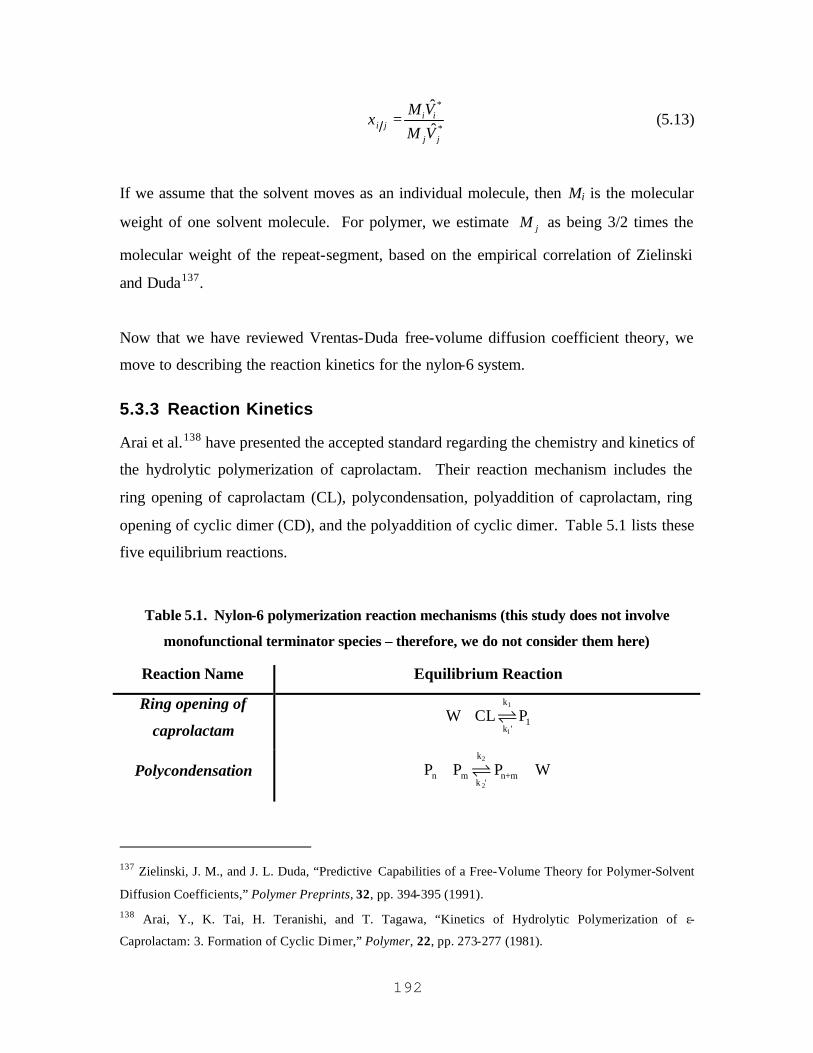
192
*
*
ˆˆ
i ii j
j j
M VM V
ξ = (5.13)
If we assume that the solvent moves as an individual molecule, then Mi is the molecular
weight of one solvent molecule. For polymer, we estimate jM as being 3/2 times the
molecular weight of the repeat-segment, based on the empirical correlation of Zielinski
and Duda137.
Now that we have reviewed Vrentas-Duda free-volume diffusion coefficient theory, we
move to describing the reaction kinetics for the nylon-6 system.
5.3.3 Reaction Kinetics
Arai et al.138 have presented the accepted standard regarding the chemistry and kinetics of
the hydrolytic polymerization of caprolactam. Their reaction mechanism includes the
ring opening of caprolactam (CL), polycondensation, polyaddition of caprolactam, ring
opening of cyclic dimer (CD), and the polyaddition of cyclic dimer. Table 5.1 lists these
five equilibrium reactions.
Table 5.1. Nylon-6 polymerization reaction mechanisms (this study does not involve
monofunctional terminator species – therefore, we do not consider them here)
Reaction Name Equilibrium Reaction
Ring opening of
caprolactam
1
1
k
1k '
W CL P+ �
Polycondensation 2
2
k
n m n+mk '
P P P W+ +�
137 Zielinski, J. M., and J. L. Duda, “Predictive Capabilities of a Free-Volume Theory for Polymer-Solvent
Diffusion Coefficients,” Polymer Preprints, 32, pp. 394-395 (1991). 138 Arai, Y., K. Tai, H. Teranishi, and T. Tagawa, “Kinetics of Hydrolytic Polymerization of ε-
Caprolactam: 3. Formation of Cyclic Dimer,” Polymer, 22, pp. 273-277 (1981).

193
Polyaddition of
caprolactam
3
3
k
n n+1k '
CL P P+ �
Ring opening of
cyclic dimer
4
4
k
2k '
W CD P+ �
Polyaddition of cyclic
dimer
5
5
k
n n+2k '
CD P P+ �
*P1 is aminocaproic acid, Pn is nylon-6 with a degree of polymerization n.
For sake of simplicity, we ignore the formation of cyclics higher than two.
Table 5.2 gives the accompanying rate constants ki, again from Arai et al139.
Table 5.2. Rate constants for the equilibrium reactions in Table 5.1
Rate constant expression
[ ] [ ]( )
00
1
exp
exp
ii i
cc ii
Ek A
RT
EA T COOH P
RT
= −
+ − − +
Equilibrium constant expression exp'
iii
ii
HSk TKk R
∆ ∆ − = =
i 0
kg/mol-siA
0
J/moliE
2 2kg /mol -s
ciA
J/mol
ciE
J/moliH∆
J/mol-K
iS∆
1 1.66E+02 8.32E+04 1.20E+04 7.87E+04 8.03E+03 -33.01
2 5.26E+06 9.74E+04 3.37E+06 8.65E+04 -
2.49E+04 3.951
3 7.93E+05 9.56E+04 4.55E+06 8.42E+04 -
1.69E+04 -29.08
139 Arai, Y., K. Tai, H. Teranishi, and T. Tagawa, “Kinetics of Hydrolytic Polymerization of ε-
Caprolactam: 3. Formation of Cyclic Dimer,” Polymer, 22, pp. 273-277 (1981).

194
4 2.38E+08 1.76E+05 6.47E+08 1.57E+05 -
4.02E+04 -60.79
5 7.14E+04 8.92E+04 8.36E+05 8.54E+04 -
1.33E+04 2.439
We use Polymers Plus and Aspen Dynamics software (Aspen Technology, Cambridge,
MA) to simulate this reaction/diffusion process, although our methodology is equally
applicable in any comparable polymer simulation software. These software tools use a
segment approach for simulating polymers in this reaction set; Table 5.3 shows the
conventional species and segment definitions.
Table 5.3. Component/segment definitions used for simulating nylon-6 polymerization
using Aspen Tech’s step-growth polymerization model140
Component/Segment Name Molecular Structure
Conventional components
Water H2O
Caprolactam C6H11NO
Amino caproic acid (P1) C6H13NO2
Oligomers and polymers
Cyclic dimer C12H22N2O2
Nylon-6 C6H11NO
Polymeric segments
Terminal amine group (T-NH2) C6H12NO
Terminal carboxylic acid group (T-
COOH) C6H12NO2
Bound nylon 6 group (B-ACA) C6H11NO
We re-write the equilibrium reactions in terms of the segment definitions:
140 David Tremblay, Aspen Technology, Cambridge, MA. Personal communication, 2003.

195
Table 5.4. Equilibrium reactions using segment approach
Equilibrium Reaction Reaction Rate
Ring-opening of Caprolactam (1
1
k
1k '
W CL P+ � )
1
1 1 1
k
k ' = k K
1
CL + W
P
�����⇀↽�����
[ ][ ][ ]
1 1
1 1'
R k CL W
k P
=
−
Polycondensation (2
2
k
n m n+mk '
P P P W+ +� )
2
2 2 2
k1 1 k '=k K
P + P
T-COOH:T-NH2 + W
������⇀↽������ [ ][ ][ ]
22 2 1
2 2'
R k P
k P W
=
−
2
2 2 2
k1 k '=k K
P + T-COOH
T-COOH:B-ACA + W
������⇀↽������
[ ][ ]
[ ][ ] [ ][ ] [ ]
3 2 1
2 '2
R k P T COOH
B ACAk W T COOH
B ACA T NH
= −
−− − − + −
2
2 2 2
k1 k '=k K
T-NH2 + P
T-NH2:B-ACA + W
������⇀↽������
[ ][ ]
[ ][ ] [ ][ ] [ ]
4 2 1
2
2
' 2
R k T NH P
B ACAk W T NH
B ACA T COOH
= −
−− − − + −
2
2 2 2
k
k '=k KT-NH2 + T-COOH
B-ACA:B-ACA + W
������⇀↽������
[ ][ ][ ][ ]
[ ][ ] [ ]
5 2
2
2
'
2
R k T NH T COOH
k W B ACA
B ACAB ACA T NH
= − −
− −
− − + −
Polyaddition of Caprolactam (3
3
k
n n+1k '
CL P P+ � )
3
3 3 3
k1 k '=k K
P + CL
T-NH2:T-COOH
�����⇀�↽������ [ ][ ][ ]
6 3 1
3 2'
R k P CL
k P
=
−
3
3 3 3
k
k '=k KT-NH2 + CL
T-NH2:B-ACA
�����⇀�↽������
[ ][ ]
[ ] [ ][ ] [ ]
7 3
3
2
' 2
R k T NH CL
B ACAk T NH
B ACA T COOH
= −
−− − − + −
Ring-opening of Cyclic Dimer (4
4
k
2k '
W CD P+ � )
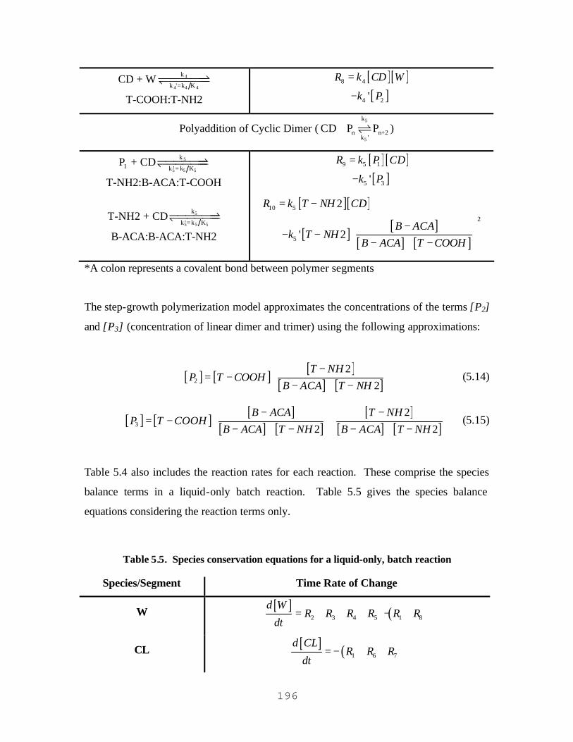
196
4
4 4 4
k
k '=k KCD + W
T-COOH:T-NH2
������⇀↽������ [ ][ ][ ]
8 4
4 2'
R k CD W
k P
=
−
Polyaddition of Cyclic Dimer (5
5
k
n n+2k '
CD P P+ � )
5
5 5 5
k1 k ' = k K
P + CD
T-NH2:B-ACA:T-COOH
�����⇀�↽������ [ ][ ][ ]
9 5 1
5 3'
R k P CD
k P
=
−
5
5 5 5
k
k ' = k KT-NH2 + CD
B-ACA:B-ACA:T-NH2
�����⇀�↽������
[ ][ ]
[ ] [ ][ ] [ ]
10 5
2
5
2
' 2
R k T NH CD
B ACAk T NH
B ACA T COOH
= −
−− − − + −
*A colon represents a covalent bond between polymer segments
The step-growth polymerization model approximates the concentrations of the terms [P2]
and [P3] (concentration of linear dimer and trimer) using the following approximations:
[ ] [ ] [ ][ ] [ ]2
22
T NHP T COOH
B ACA T NH
−= − − + −
(5.14)
[ ] [ ] [ ][ ] [ ]
[ ][ ] [ ]3
22 2
B ACA T NHP T COOH
B ACA T NH B ACA T NH
− −= − − + − − + −
(5.15)
Table 5.4 also includes the reaction rates for each reaction. These comprise the species
balance terms in a liquid-only batch reaction. Table 5.5 gives the species balance
equations considering the reaction terms only.
Table 5.5. Species conservation equations for a liquid-only, batch reaction
Species/Segment Time Rate of Change
W [ ] ( )2 3 4 5 1 8
d WR R R R R R
dt= + + + − +
CL [ ] ( )1 6 7
d CLR R R
dt= − + +
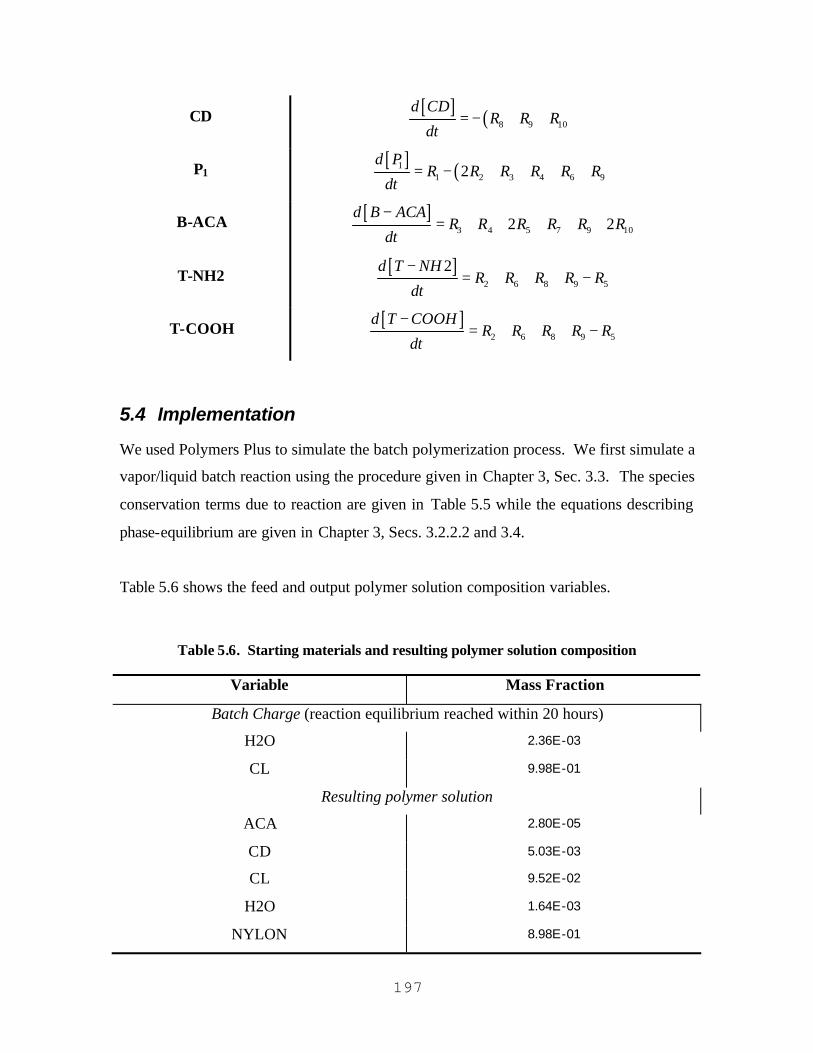
197
CD [ ] ( )8 9 10
d CDR R R
dt= − + +
P1 [ ] ( )1
1 2 3 4 6 92d P
R R R R R Rdt
= − + + + +
B-ACA [ ]3 4 5 7 9 102 2
d B ACAR R R R R R
dt
−= + + + + +
T-NH2 [ ]2 6 8 9 5
2d T NHR R R R R
dt
−= + + + −
T-COOH [ ]2 6 8 9 5
d T COOHR R R R R
dt
−= + + + −
5.4 Implementation
We used Polymers Plus to simulate the batch polymerization process. We first simulate a
vapor/liquid batch reaction using the procedure given in Chapter 3, Sec. 3.3. The species
conservation terms due to reaction are given in Table 5.5 while the equations describing
phase-equilibrium are given in Chapter 3, Secs. 3.2.2.2 and 3.4.
Table 5.6 shows the feed and output polymer solution composition variables.
Table 5.6. Starting materials and resulting polymer solution composition
Variable Mass Fraction
Batch Charge (reaction equilibrium reached within 20 hours)
H2O 2.36E-03
CL 9.98E-01
Resulting polymer solution
ACA 2.80E-05
CD 5.03E-03
CL 9.52E-02
H2O 1.64E-03
NYLON 8.98E-01

198
Nagasubramanian and Reimschuessel did not give the H2O/CL ratio for their charging
materials – we back-calculated that value by matching the reported final polymer
molecular weight. The final number-average degree of polymerization is about 200.
After we generate the concentrated polymer solution for use in this study, we use a
continuous-stirred-tank reactor model in Aspen Dynamics to simulate the batch
diffusion/reaction process. We shut off the liquid feed and product streams for the
reactor and only consider a continuous helium feed stream and outlet vapor stream. We
implement penetration theory (Eq. (5.2)) using the customization features available in
AD.
The initial conditions are those listed in Table 5.6. The mass transfer boundary condition
is computed by assuming thermodynamic equilibrium between the liquid interface and
the vapor phase (Eq. (5.4)).
The reactor is a vertical cylinder with a flat head and heel (see Figure 5.1). The diameter
is 0.055 m, the height is 0.198 m, and the liquid level is 0.07 m. The helium injection
rate is 2.50E-06 m3/s. The diffusion experiment was carried out at 265 °C (operating
conditions from Nagasubramanian and Reimschuessel141).
5.5 Results and Discussion
5.5.1 Estimates of Free-Volume Parameters
We first find the viscosity/temperature equations for water, caprolactam, and nylon-6.
Daubert and Danner142 give the viscosity expressions for water and caprolactam:
141 Nagasubramanian, K., and H. K. Reimschuessel, “Diffusion of Water and Caprolactam in Nylon-6
Melts,” Journal of Applied Polymer Science, 17, pp. 1663-1677 (1973). 142 Daubert, T. E., and R. P. Danner, Physical and Thermodynamic Properties of Pure Chemicals. Data
Compilation, Volume 3 , Hemisphere Publishing Corporation, New York (1989).
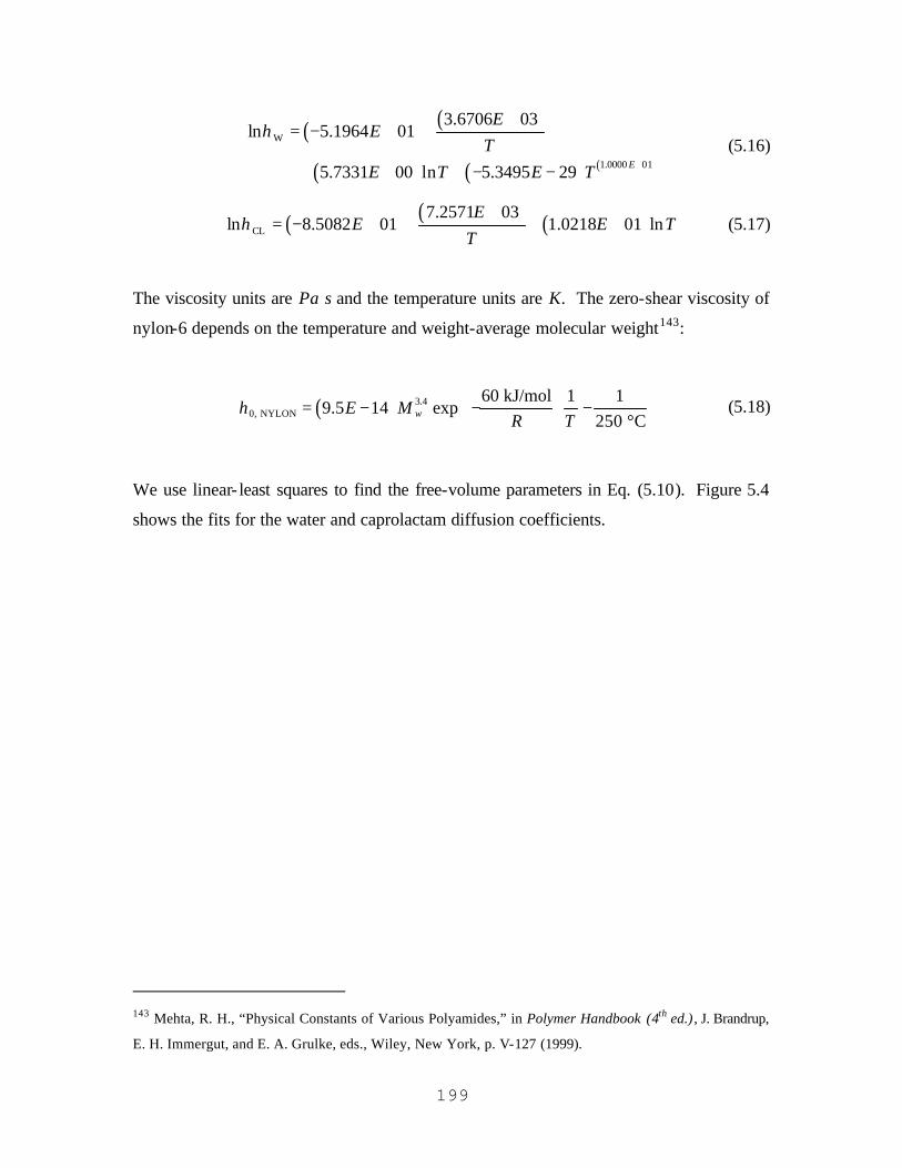
199
( ) ( )
( ) ( ) ( )
W
1.0000 01
3.6706 03ln 5.1964 01
5.7331 00 ln 5.3495 29 E
EE
TE T E T
η
+
+= − + +
+ + + − − (5.16)
( ) ( ) ( )CL
7.2571 03ln 8.5082 01 1.0218 01 ln
EE E T
Tη
+= − + + + + (5.17)
The viscosity units are Pa s and the temperature units are K. The zero-shear viscosity of
nylon-6 depends on the temperature and weight-average molecular weight143:
( ) 3.40, NYLON
60 kJ/mol 1 19.5 14 exp
250 °CwE MR T
η
= − − −
(5.18)
We use linear- least squares to find the free-volume parameters in Eq. (5.10). Figure 5.4
shows the fits for the water and caprolactam diffusion coefficients.
143 Mehta, R. H., “Physical Constants of Various Polyamides,” in Polymer Handbook (4th ed.) , J. Brandrup,
E. H. Immergut, and E. A. Grulke, eds., Wiley, New York, p. V-127 (1999).
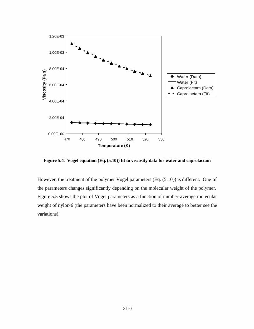
200
0.00E+00
2.00E-04
4.00E-04
6.00E-04
8.00E-04
1.00E-03
1.20E-03
470 480 490 500 510 520 530
Temperature (K)
Vis
cosi
ty (
Pa
s)
Water (Data)Water (Fit)Caprolactam (Data)Caprolactam (Fit)
Figure 5.4. Vogel equation (Eq. (5.10)) fit to viscosity data for water and caprolactam
However, the treatment of the polymer Vogel parameters (Eq. (5.10)) is different. One of
the parameters changes significantly depending on the molecular weight of the polymer.
Figure 5.5 shows the plot of Vogel parameters as a function of number-average molecular
weight of nylon-6 (the parameters have been normalized to their average to better see the
variations).

201
0.75
0.85
0.95
1.05
1.15
1.25
10000 12000 14000 16000 18000 20000 22000
Number-Average Molecular Weight (g/mol)
No
rmal
ized
Fre
e-V
olu
me
Par
amet
er
ABC
Figure 5.5. Normalized Vogel parameters (Eq. (5.10)) as a function of nylon-6 molecular
weight
We have assumed that the polydispersity is two, the most-probable (or Schultz-Flory)
distribution.
Significant mass-transfer resistance typically occurs in nylon-6 reactors that handle
polymer of a number-average molecular weight of 12,000 g/mol and higher. Therefore,
the variation in the B and C parameters is negligible. The A parameter changes
substantially throughout the molecular weight range; however, this does not matter
because we do not use A in the diffusion coefficient theory. We use the average of the B
and C parameter throughout the number-average molecular weight range of 12,000 to
22,000 g/mol. Table 5.7 contains the pertinent free volume parameters.

202
Table 5.7. Vogel parameters for water, caprolactam, and nylon-6
Species A B (K) C (K)
Water -1.09E+01 8.15E+02 -6.39E+01
Caprolactam -9.42E+00 6.43E+02 -2.27E+02
Nylon-6* -6.76E+00 to -4.67E+00 4.77E+03 -9.18E+01
*Values are for the number-average molecular weight range of 12,000 to 22,000 g/mol.
A parameter is the range, while the B and C parameters are averages over the range.
Next, we compute the pre-exponential factor D01 for both water and caprolactam. We
first need the critical molar volume, molecular weight, and specific volumes for water
and caprolactam. Table 5.8 contains the molecular weights and critical molar volumes,
from Daubert and Danner144.
Table 5.8. Molecular weight and critical molar volume for water and caprolactam145
Species Molecular Weight (g/mol) Critical Molar Volume (m3/kmol)
Water 18.015 0.05595
Caprolactam 113.159 0.40200
The specific volume of the solvent comes from the DIPPR equation146, which is a
modification of the Rackett equation for liquid molar volume:
( )( )
0
1 1ˆ
Dii
ii T C
i i
MV
A B− + −
= (5.19)
144 Daubert, T. E., and R. P. Danner, Physical and Thermodynamic Properties of Pure Chemicals. Data
Compilation, Volume 3 , Hemisphere Publishing Corporation, New York (1989). 145 Daubert, T. E., and R. P. Danner, Physical and Thermodynamic Properties of Pure Chemicals. Data
Compilation, Volume 3 , Hemisphere Publishing Corporation, New York (1989). 146 Daubert, T. E., and R. P. Danner, Physical and Thermodynamic Properties of Pure Chemicals. Data
Compilation, Volume 3 , Hemisphere Publishing Corporation, New York (1989).
203
The denominator is the liquid density (kmol/m3) and the numerator is the molecular
weight (kg/kmol). The specific volume therefore has units of m3 /kg. Table 5.9 contains
the specific volume parameters.
Table 5.9. Specific volume DIPPR parameters for water and caprolactam147
Species A B C D
Water 5.4590E+00 3.0542E-01 6.4713E+02 8.1000E-02
Caprolactam 7.1180E-01 2.5400E-01 8.0600E+02 2.8570E-01
The combination of these pure-component properties (Table 5.8 and Table 5.9) along
with the Vogel parameters allow us to generate plots for the pre-exponential factor as a
function of temperature for water and caprolactam (Figure 5.6 and Figure 5.7).
147 Daubert, T. E., and R. P. Danner, Physical and Thermodynamic Properties of Pure Chemicals. Data
Compilation, Volume 3 , Hemisphere Publishing Corporation, New York (1989).
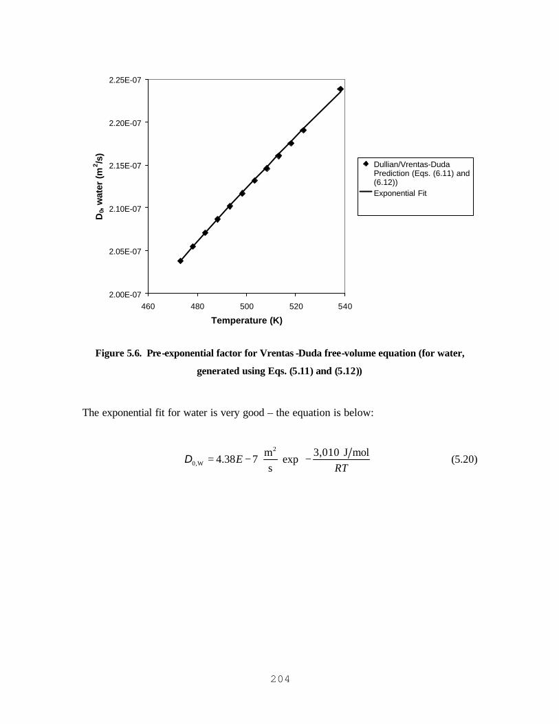
204
2.00E-07
2.05E-07
2.10E-07
2.15E-07
2.20E-07
2.25E-07
460 480 500 520 540
Temperature (K)
D0,
wat
er (
m2 /s
)
Dullian/Vrentas-DudaPrediction (Eqs. (6.11) and(6.12))Exponential Fit
Figure 5.6. Pre-exponential factor for Vrentas -Duda free-volume equation (for water,
generated using Eqs. (5.11) and (5.12))
The exponential fit for water is very good – the equation is below:
2
0,Wm 3,010 J mol
4.38 7 exps
ERT
= − −
D (5.20)
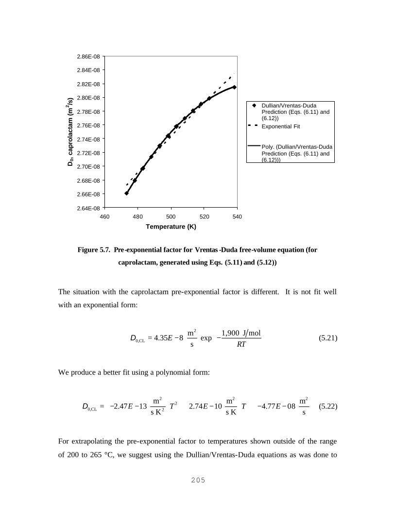
205
2.64E-08
2.66E-08
2.68E-08
2.70E-08
2.72E-08
2.74E-08
2.76E-08
2.78E-08
2.80E-08
2.82E-08
2.84E-08
2.86E-08
460 480 500 520 540
Temperature (K)
D0,
cap
rola
ctam
(m
2 /s)
Dullian/Vrentas-DudaPrediction (Eqs. (6.11) and(6.12))Exponential Fit
Poly. (Dullian/Vrentas-DudaPrediction (Eqs. (6.11) and(6.12)))
Figure 5.7. Pre-exponential factor for Vrentas -Duda free-volume equation (for
caprolactam, generated using Eqs. (5.11) and (5.12))
The situation with the caprolactam pre-exponential factor is different. It is not fit well
with an exponential form:
2
0,CLm 1,900 J mol
4.35 8 exps
ERT
= − −
D (5.21)
We produce a better fit using a polynomial form:
2 2 2
20,CL 2
m m m2.47 13 2.74 10 4.77 08
s K s K sE T E T E
= − − + − + − −
D (5.22)
For extrapolating the pre-exponential factor to temperatures shown outside of the range
of 200 to 265 °C, we suggest using the Dullian/Vrentas-Duda equations as was done to

206
generate the predictions in the first place. The extrapability of Eq. (5.22) is questionable
because it is not based on first principles.
Lastly, we estimate the ratio of the molar volume ratio of jumping units. We first need to
estimate the specific hole free-volume for each species *iV . We do so using Blitz’s rule,
as outlined in Haward148:
*ˆ ˆ0.91 mpi iV V= (5.23)
ˆ mpiV is the solid density of species i at the melting point. We find these for water and
caprolactam in Daubert and Danner149. For polymer, we use the crystalline density of
nylon-6 from the Polymer Handbook150 as the value for the specific hole free-volume.
Table 5.10 contains the parameters that we use to compute the ratio of jumping units.
Table 5.10. Free-volume parameters for water, caprolactam, and nylon-6 repeat segment151
( *iV generated using Eq. (5.23) for water and caprolactam; for nylon-6, we used the
crystalline density)
Species Mi (kg/mol) ˆ mpiV (m3/kg) *
iV (m3/kg)
Water 0.018015 1.09E-03 9.93E-04
Caprolactam 0.113159 9.12E-04 8.30E-04
Nylon-6 repeat segment 0.113159 N. A. 8.13E-04
148 Haward, R. N., “Occupied Volume of Liquids and Polymers,” Journal of Macromolecular Science.
Reviews in Macromolecular Chemistry, C4(2), pp. 191-242 (1970). 149 Daubert, T. E., and R. P. Danner, Physical and Thermodynamic Properties of Pure Chemicals. Data
Compilation, Volume 3 , Hemisphere Publishing Corporation, New York (1989). 150 Mehta, R. H., “Physical Constants of Various Polyamides,” in Polymer Handbook (4th ed.) , J. Brandrup,
E. H. Immergut, and E. A. Grulke, eds., Wiley, New York, p. V-124 (1999). 151 Daubert, T. E., and R. P. Danner, Physical and Thermodynamic Properties of Pure Chemicals. Data
Compilation, Volume 3 , Hemisphere Publishing Corporation, New York (1989).
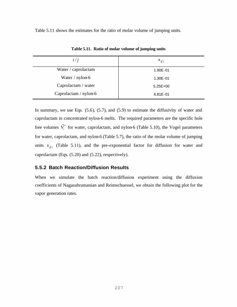
207
Table 5.11 shows the estimates for the ratio of molar volume of jumping units.
Table 5.11. Ratio of molar volume of jumping units
i / j i jξ
Water / caprolactam 1.90E-01
Water / nylon-6 1.30E-01
Caprolactam / water 5.25E+00
Caprolactam / nylon-6 6.81E-01
In summary, we use Eqs. (5.6), (5.7), and (5.9) to estimate the diffusivity of water and
caprolactam in concentrated nylon-6 melts. The required parameters are the specific hole
free volumes *iV for water, caprolactam, and nylon-6 (Table 5.10), the Vogel parameters
for water, caprolactam, and nylon-6 (Table 5.7), the ratio of the molar volume of jumping
units i jξ (Table 5.11), and the pre-exponential factor for diffusion for water and
caprolactam (Eqs. (5.20) and (5.22), respectively).
5.5.2 Batch Reaction/Diffusion Results
When we simulate the batch reaction/diffusion experiment using the diffusion
coefficients of Nagasubramanian and Reimschuessel, we obtain the following plot for the
vapor generation rates.
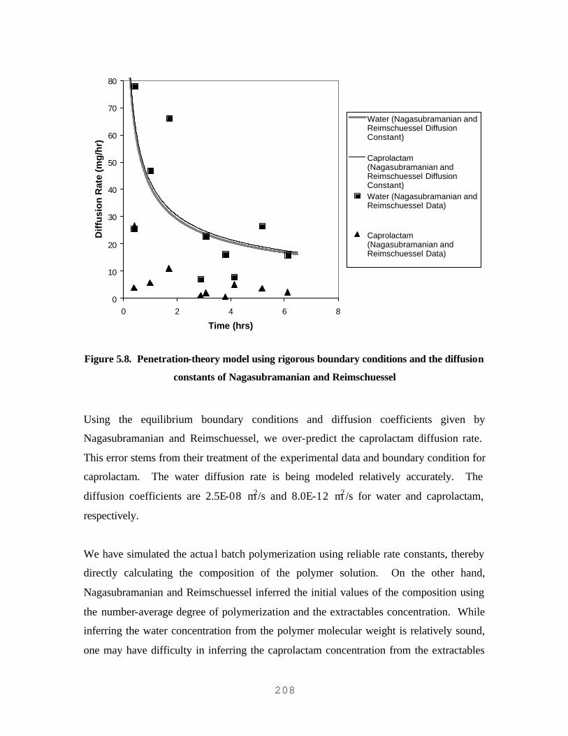
208
0
10
20
30
40
50
60
70
80
0 2 4 6 8
Time (hrs)
Dif
fusi
on
Rat
e (m
g/h
r)
Water (Nagasubramanian andReimschuessel DiffusionConstant)
Caprolactam(Nagasubramanian andReimschuessel DiffusionConstant)Water (Nagasubramanian andReimschuessel Data)
Caprolactam(Nagasubramanian andReimschuessel Data)
Figure 5.8. Penetration-theory model using rigorous boundary conditions and the diffusion
constants of Nagasubramanian and Reimschuessel
Using the equilibrium boundary conditions and diffusion coefficients given by
Nagasubramanian and Reimschuessel, we over-predict the caprolactam diffusion rate.
This error stems from their treatment of the experimental data and boundary condition for
caprolactam. The water diffusion rate is being modeled relatively accurately. The
diffusion coefficients are 2.5E-08 m2/s and 8.0E-12 m2 /s for water and caprolactam,
respectively.
We have simulated the actua l batch polymerization using reliable rate constants, thereby
directly calculating the composition of the polymer solution. On the other hand,
Nagasubramanian and Reimschuessel inferred the initial values of the composition using
the number-average degree of polymerization and the extractables concentration. While
inferring the water concentration from the polymer molecular weight is relatively sound,
one may have difficulty in inferring the caprolactam concentration from the extractables

209
concentration. This is because the extractables include a significant and unknown
fraction of linear and cyclic oligomers.
We found that the boundary condition predicted using equilibrium theory (Eq. (5.4))
actually changes considerably throughout the polymerization/diffusion. The water
boundary condition changes from 1.79E-04 kmol/m3 to 1.04E-05, while the caprolactam
boundary condition changes from 1.69E-03 kmol/m3 to 9.87E-05 over the six-hour
experiment. This is in contrast to Nagasubramanian and Reimschuessel’s work, in which
they fix the value of the interfacial boundary condition to extrapolated and regressed
values (outlined in Sec. 5.2).
We now simulate the diffusion/reaction experiment using diffusion coefficients from
Vrentas-Duda free-volume theory (Figure 5.9). We estimate the required parameters
using only viscosity and density data (Sec. 5.5.1).

210
0
10
20
30
40
50
60
70
80
0 2 4 6 8
Time (hrs)
Dif
fusi
on
Rat
e (m
g/h
r)
Water (Vrentas-DudaPrediction)
Caprolactam (Vrentas-DudaPrediction)
Water (Nagasubramanian andReimschuessel Data)
Caprolactam(Nagasubramanian andReimschuessel Data)
Figure 5.9. Vrentas -Duda free-volume model for diffusion coefficient along with
penetration theory and equilibrium boundary conditions (Vrentas -Duda parameters
regressed from viscosity and density data only).
The predictions are decent considering that the diffusion coefficients were predicted a
priori and not fit to any diffusion data. The predicted rate of water diffusion is excellent;
however, the predicted rate of diffusion for caprolactam devolatization is too high when
compared with the experimental data152. This is most likely because the Vrentas-Duda
model has made an error in approximating the concentration dependence of the pure
caprolactam diffusion coefficients. The predicted diffusion coefficients are 7.76E-08
m2/s and 1.09E-10 m2/s for water and caprolactam in this solution, respectively. The
self-diffusion coefficients, according to the Dullian equation (Eq. (5.11)), are 4.01E-08
m2/s and 3.56E-09 m2/s for water and caprolactam, respectively.
152 Nagasubramanian, K., and H. K. Reimschuessel, “Diffusion of Water and Caprolactam in Nylon-6
Melts,” Journal of Applied Polymer Science, 17, pp. 1663-1677 (1973).

211
In order to improve the predictions of the Vrentas-Duda model, we focus on the most
controversial parameter in the model – the ratio of the jumping unit during diffusion
i jξ −153. We have four such parameters: W-CL W-NYLON CL-W CL-NYLON, , , and ξ ξ ξ ξ . When we
remember the definition of these parameters, that they are the ratio of the jumping units
of i and j, we can reduce these four parameters down to two independent parameters:
W-NYLONW-CL
CL-NYLON
ξξ
ξ= (5.24)
CL-NYLONCL-W
W-NYLON W-CL
1ξξ
ξ ξ= = (5.25)
We manipulate the parameters W-NYLONξ and CL-NYLONξ from their original values (Table
5.11) in order to improve the fit to the data. We seek to zero the following error function:
( )model data
dataError i i
i
E E
E
−= (5.26)
We arrive at the final fit to the data (Figure 5.10).
153 Zielinski, J. M., and J. L. Duda, “Predictive Capabilities of a Free-Volume Theory for Polymer-Solvent
Diffusion Coefficients,” Polymer Preprints, 32, pp. 394-395 (1991).
212
0
10
20
30
40
50
60
70
80
0 2 4 6 8
Time (hrs)
Dif
fusi
on
Rat
e (m
g/h
r)
Water (Vrentas-Duda)
Caprolactam (Vrentas-Duda)
Water (Nagasubramanian andReimschuessel Data)
Caprolactam(Nagasubramanian andReimschuessel Data)
Figure 5.10. Vrentas -Duda free-volume model for diffusion coefficient along with
penetration theory and equilibrium boundary conditions (Vrentas -Duda adjusted to fit
diffusion data).
The fitted parameters are H2O-NYLONξ equal to 8.54E-02 (0.657 times the original value)
and CL-NYLONξ equal to 1.55 (2.27 times the original value). The diffusion coefficient of
water at these conditions is 1.17E-07 m2/s and for caprolactam 2.31E-13 m2/s.
This brings us to an important point regarding the composition dependence of the
diffusion coefficient. It appears that composition dependence cannot be ignored in
transforming the self-diffusion coefficient of water and caprolactam into the respective
diffusion coefficient in a concentrated nylon-6 solution. For example, the diffusion
coefficient of caprolactam has decreased by four orders of magnitude under the original
Dullian equation (Eq. (5.11)) prediction for the self-diffusion coefficient. One may argue
that the composition dependence can be ignored over a small region of the composition
range – however, we recommend theoretically testing this assumption because
213
composition appears in an exponential term according to the Vrentas-Duda equation
(Eqs. (5.6) and (5.7)) and may exert a strong influence. In our case, we regress data from
a diffusion experiment in which the solution contains ca. 9% (by mass) caprolactam – we
suspect that extrapolating these results to ca. 1% caprolactam (as would be required to
simulate a continuous finishing operation that produces ready-to-spin polymer melt like
the one disclosed in Yates et al.154) would require some kind of composition correction.
However, if one expects to simulate only those solutions at ca. 9% caprolactam, then the
diffusion coefficients given in the previous paragraph should be adequate.
In summary, Table 5.12 shows the diffusion coefficient values that we have encountered
thus far.
Table 5.12. Comparison of diffusion coefficient values encountered in this study (values in
parenthesis are in units of cm2/s)
Species
Nagasubramanian
and Reimscheussel
Diffusion
Coefficient (m2/s)
Vrentas/Duda
Uncorrected
Diffusion
Coefficient (m2/s)
Vrentas/Duda
Corrected Diffusion
Coefficient (m2/s)
Water 2.50E-08 (2.50E-04) 7.76E-08 (7.76E-04) 1.17E-07 (1.17E-03)
Caprolactam 8.00E-12 (8.00E-08) 1.09E-10 (1.09E-06) 2.31E-13 (2.31E-09)
We summarize the final diffusion coefficient model used to generate the fits in Figure
5.10.
µ µ µ
µ* * *W CL NYLONW CL W C L NYLON W NYLON
W 0,W
( )exp
FH
V V V
V
ω ω ξ ω ξ
γ
+ + = −
D D (5.27)
154 Yates, S. L., C. J. Cole, A. H. Wiesner, and J. W. Wagner, “Two-Stage Hydrolysis Process for the
Preparation of Nylon-6,” United States Patent #4,310,659 (1982).
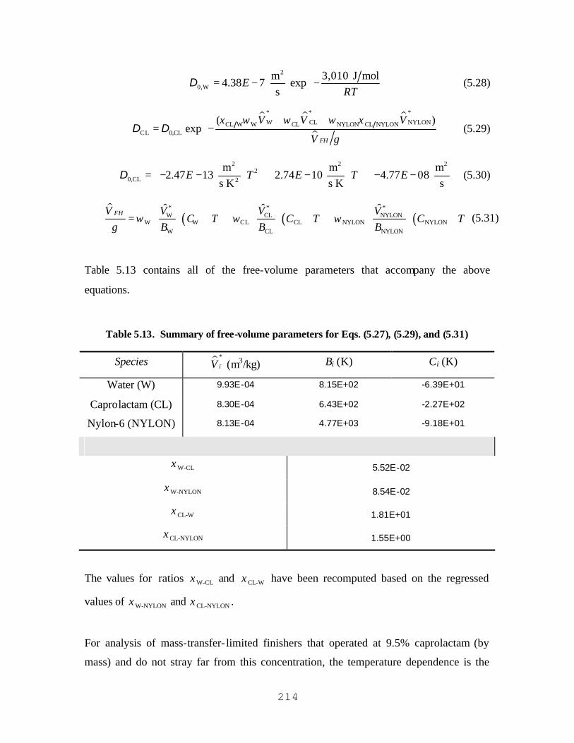
214
2
0,Wm 3,010 J mol
4.38 7 exps
ERT
= − −
D (5.28)
µ µ µ
µ* * *W CL NYLONCL W W CL NYLON CL NYLON
CL 0,CL
( )exp
FH
V V V
V
ξ ω ω ω ξ
γ
+ + = −
D D (5.29)
2 2 2
20,CL 2
m m m2.47 13 2.74 10 4.77 08
s K s K sE T E T E
= − − + − + − −
D (5.30)
µ
( ) ( ) ( )* * *
W CL NYLONW W CL CL NYLON NYLON
W CL NYLON
ˆ ˆ ˆFH V V VVC T C T C T
B B Bω ω ω
γ
= + + + + +
(5.31)
Table 5.13 contains all of the free-volume parameters that accompany the above
equations.
Table 5.13. Summary of free-volume parameters for Eqs. (5.27), (5.29), and (5.31)
Species µ *iV (m3/kg) Bi (K) Ci (K)
Water (W) 9.93E-04 8.15E+02 -6.39E+01
Caprolactam (CL) 8.30E-04 6.43E+02 -2.27E+02
Nylon-6 (NYLON) 8.13E-04 4.77E+03 -9.18E+01
W-CLξ 5.52E-02
W-NYLONξ 8.54E-02
CL-Wξ 1.81E+01
CL-NYLONξ 1.55E+00
The values for ratios W-CLξ and CL-Wξ have been recomputed based on the regressed
values of W-NYLONξ and CL-NYLONξ .
For analysis of mass-transfer- limited finishers that operated at 9.5% caprolactam (by
mass) and do not stray far from this concentration, the temperature dependence is the

215
only important factor, and the concentration dependence can be ignored. We estimate the
equation containing only temperature dependence by using the diffusion coefficients
regressed from the data (Vrentas/Duda corrected in Table 5.12) and the activation
energies contained in Eqs. (5.20) and (5.21):
2
Wm 3,010 J mol
2.29 7 exps
ERT
= − −
D (5.32)
2
CLm 1,900 J mol
3.53 13 exps
ERT
= − −
D (5.33)
These expressions must be used with caution – the Vrentas-Duda theory predicts that at
8% caprolactam, the diffusion coefficient of water has decreased by 3% and that for
caprolactam has decreased by 46%.
5.6 Application of Diffusivity Model
Let us consider the design of a simple batch process for produc ing nylon-6. We start
with a batch reactor that is 2.4 m in diameter and 4.8 m in height. It is vertically oriented
with an elliptical geometry. The vessel is 85% full and has a volume of approximately
21.7 m3, ignoring the added volume due to the elliptical head and heel. We charge the
reactor with 18,000 kg of caprolactam and 180 kg of water. We simulate the reactor for 6
hours at 260 °C using the same Polymer Plus model described in Sec. 5.4. Figure 5.11
shows the batch reactor profiles.
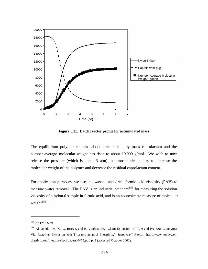
216
0
2000
4000
6000
8000
10000
12000
14000
16000
18000
20000
0 1 2 3 4 5 6 7
Time (hr)
Nylon-6 (kg)
Caprolactam (kg)
Number-Average MolecularWeight (g/mol)
Figure 5.11. Batch reactor profile for accumulated mass
The equilibrium polymer contains about nine percent by mass caprolactam and the
number-average molecular weight has risen to about 10,000 g/mol. We wish to now
release the pressure (which is about 3 atm) to atmospheric and try to increase the
molecular weight of the polymer and decrease the residual caprolactam content.
For application purposes, we use the washed-and-dried formic-acid viscosity (FAV) to
measure water removal. The FAV is an industrial standard155 for measuring the solution
viscosity of a nylon-6 sample in formic acid, and is an approximate measure of molecular
weight156:
155 ASTM D789 156 Akkapeddi, M. K., C. Brown, and B. Vanbuskirk, “Chain Extension of PA-6 and PA-6/66 Copolymer
Via Reactive Extrusion with Triscaprolactamyl Phosphite,” Honeywell Report, http://www.honeywell-
plastics.com/literature/techpapers/0475.pdf, p. 3 (accessed October 2002).

217
( ) ( )2.159.38 9 2 nFAV E M= − (5.34)
The formic-acid viscosity is a relative viscosity – the ratio of the solution viscosity to the
viscosity of pure formic acid. It is therefore dimensionless.
Let us consider the evaporation rate equation for our process once again:
int , , *2 i ii i L i Lsat
c i
y PE A C v
t Pπ
= −
D (5.35)
, *i Lv is the molar volume of the liquid phase at the interface. There are three primary
ways in which we can enhance devolatization (i.e., increase Ei) without changing the
temperature: we can increase the interfacial surface area intA , we can decrease the system
pressure P, or we can decrease our average contact time ct . The average contact time is
influenced by mixing effects – the more vigorous the stirring, the less time between
surface renewal events. However, the more viscous the solution, the more time goes by
before surface renewal.
If we adjust the reactor temperature, then we influence the viscosity, the diffusion
coefficient, and the vapor pressure of the species. Higher temperature increases the
diffusion coefficient and the vapor pressure – both of these effects enhance mass transfer.
Increasing the temperature also decreases the viscosity, thereby enhancing the frequency
of surface renewal effects during agitation.
Let us first consider two cases: one in which we are operating the reactor at atmospheric
pressure with no agitation and one in which we are able to renew the surface every
minute using mixing. Renewing the surface area every minute means that the time term
in Eq. (5.35) is reset every minute. The surface area is 4.52 m2 and the temperature is
260 °C. Figure 5.12 shows the FAV build and caprolactam content for these two cases.

218
0.9
1
1.1
1.2
1.3
1.4
1.5
1.6
0 1 2 3 4 5 6 7
Time (hrs)
Val
ue
No
rmal
ized
to
Init
ial V
alu
e
CL (Base)FAV (base)CL (Mixing)FAV (mixing)
Figure 5.12. Comparison of normalized caprolactam weight fraction (CL) and formic-acid
viscosity (FAV) profiles (CL initial value 0.0815, FAV initial value 16.7) – caprolactam
devolatization is hardly affected by surface renewal every minute caused by mixing whereas
increased water evaporation causes the FAV to rise modestly
Surface renewal through mixing increases the rate of FAV build, but does not do so
significantly. Caprolactam devolatization is not affected at all.
Keeping the mixing (surface renewal every minute), we now compare the effects of
increasing the surface area to that of vacuum. We use a vacuum of 50 mm Hg. The
surface area is increased by a factor of 2.5. This could be achieved by bubbling an inert
gas stream through the polymer melt. Figure 5.13 shows the results.
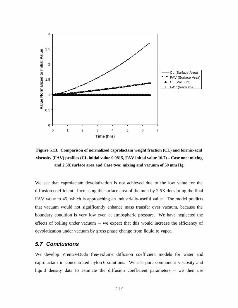
219
0
0.5
1
1.5
2
2.5
3
0 1 2 3 4 5 6 7
Time (hrs)
Val
ue
No
rmal
ized
to
Init
ial V
alu
e
CL (Surface Area)FAV (Surface Area)CL (Vacuum)FAV (Vacuum)
Figure 5.13. Comparison of normalized caprolactam weight fraction (CL) and formic-acid
viscosity (FAV) profiles (CL initial value 0.0815, FAV initial value 16.7) – Case one: mixing
and 2.5X surface area and Case two: mixing and vacuum of 50 mm Hg
We see that caprolactam devolatization is not achieved due to the low value for the
diffusion coefficient. Increasing the surface area of the melt by 2.5X does bring the final
FAV value to 45, which is approaching an industrially-useful value. The model predicts
that vacuum would not significantly enhance mass transfer over vacuum, because the
boundary condition is very low even at atmospheric pressure. We have neglected the
effects of boiling under vacuum – we expect that this would increase the efficiency of
devolatization under vacuum by gross phase change from liquid to vapor.
5.7 Conclusions
We develop Vrentas-Duda free-volume diffusion coefficient models for water and
caprolactam in concentrated nylon-6 solutions. We use pure-component viscosity and
liquid density data to estimate the diffusion coefficient parameters – we then use
220
penetration theory, the reaction kinetics of Arai et al., and devolatization data at 265 °C
and a caprolactam mass fraction of 0.1 to fine-tune the ratio of the molar volume of
jumping units for water, caprolactam, and nylon-6.
We then apply our diffusion coefficient model to analyze a typical industrial
polymerization process. We qualitatively examine the effects of increasing the interfacial
surface area, mixing, and vacuum on devolatization. We found that mixing marginally
increased the diffusion of water through the polymer melt – however, to build a high-
molecular weight polymer, we had to increase the surface area of the melt by a factor of
10. We were not able to significantly reduce the caprolactam content in the melt, even
through the use of a vacuum of 50 mm Hg. However, we neglected the effects of
solution boiling, which we expect would enhance the removal of residual monomer.

221
5.8 Nomenclature
Symbol Description Units
intA Interfacial area m2
Ai0 Pre-exponential factor for uncatalyzed
forward reaction i kg/mol-s
Aic Pre-exponential factor for catalyzed
forward reaction i kg/mol-s
,i LC Concentration of species i in the bulk liquid phase kmol/m3
, *i LC Concentration of species i at the liquid-side interface kmol/m3
iD Diffusion coefficient of species i m2/s
0,iD Pre-exponential diffusion coefficient for species i m2/s
Ei Evaporation rate for species i kmol/s
Ei0 Activation energy for uncatalyzed
forward reaction i J/mol
Eic Activation energy for catalyzed
forward reaction i J/mol
FAV Formic-acid viscosity Unitless
iH∆ Enthalpy of reaction i J/mol
Ki Equilibrium constant for reaction i Unitless
ki Forward rate constant for reaction i kg/mol-s
ki’ Reverse rate constant for reaction i kg/mol-s
,L ik a Mass-transfer coefficient for species i 1/s
Mi Molecular weight of species i kg/kmol
nM Number-average molecular weight kg/mol
P Pressure Pa sat
iP Vapor pressure of species i Pa
Px Polymer chain with degree of polymerization x N. A.
Px,y Polymer chain with degree of polymerization x and

222
termination condition y N. A.
Ri Rate equation for reaction i N. A.
iS∆ entropy of reaction i J/mol-K
T Temperature K
ct Contact time s
,c iV Critical molar volume of species i m3/mol
0iV Specific volume of species i m3/kg
LV Volume of the liquid phase m3
µFHV Specific hole free volume for the mixture m3/kg
µ *iV Specific hole free volume for species i m3/kg
xi Liquid mole fraction of species i Unitless
nx Number-average degree of polymerization Unitless
yi Vapor mole fraction of species i Unitless
γ Overlap factor for the mixture Unitless
iη Viscosity of species i Pa s
i jξ Ratio of the molar volumes of the jumping units for
species i and j Unitless
iω Weight fraction of species i Unitless
223
6 Simulation of Vacuum Reactors for Finishing Step-
Growth Polymers
Chapters 2 through 5 provide the background material for simulating mass-transfer-
limited finishing reactors. In this chapter, we conclude our analysis of nylon-6
polymerizations by developing a model for a particularly complicated class of finishing
reactors – those operating under vacuum. These reactors are complex because: (1) they
are equipped with internals which are meant to provide more interfacial surface area for
diffusion, and (2) they are operating under vacuum, causing boiling in the concentrated
polymer solution. Our model explicitly accounts for mass transfer of volatiles through
two key mechanisms: bubble nucleation under vacuum and molecular diffusion through
the vapor- liquid interface. It is an improvement over models in the past, because it
clarifies the effect of vacuum on mass transfer and also the impact of vapor bubbles on
the devolatization of a concentrated nylon-6 solution.
Chapter organization is as follows.
• 6.1 – Introduction to commercial technology for producing nylon-6
• 6.2 – Overview of finishing reactor technology
• 6.3 – Literature review for finishing reactor models
• 6.4 – Theory of vacuum-limited devolatization
• 6.5 – Implementation
• 6.6 – Model performance and comparison with previous model
• 6.7 - Conclusions
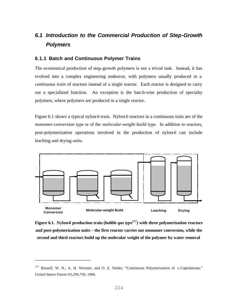
224
6.1 Introduction to the Commercial Production of Step-Growth
Polymers
6.1.1 Batch and Continuous Polymer Trains
The economical production of step-growth polymers is not a trivial task. Instead, it has
evolved into a complex engineering endeavor, with polymers usually produced in a
continuous train of reactors instead of a single reactor. Each reactor is designed to carry
out a specialized function. An exception is the batch-wise production of specialty
polymers, where polymers are produced in a single reactor.
Figure 6.1 shows a typical nylon-6 train. Nylon-6 reactors in a continuous train are of the
monomer-conversion type or of the molecular-weight-build type. In addition to reactors,
post-polymerization operations involved in the production of nylon-6 can include
leaching and drying units.
Monomer Conversion
Molecular-weight Build Leaching Drying
Figure 6.1. Nylon-6 production train (bubble-gas type157) with three polymerization reactors
and post-polymerization units – the first reactor carries out monomer conversion, while the
second and third reactors build up the molecular weight of the polymer by water removal
157 Russell, W. N., A. H. Wiesner, and O. E. Snider, “Continuous Polymerization of ε-Caprolactam,”
United States Patent #3,294,756, 1966.
225
The first polymerization kettle is operated at high pressure to keep water from vaporizing
out of the reaction mixture. A high water content in the liquid phase is necessary to drive
the reaction equilibrium in the direction of monomer conversion.
The second and third polymerization kettles are typically operated at ambient pressure.
Inert gas is bubbled through the reaction mass to remove water. This water removal
promotes molecular weight build. Lastly, the high-molecular-weight polymer must be
subjected to washing and drying in order to remove residual monomer and reaction side
products (e.g., cyclic dimer).
Instead of washing and drying the polymer in separate steps, melt trains have been
developed to combine the molecular-weight build, devolatization, and drying steps
(Figure 6.2).
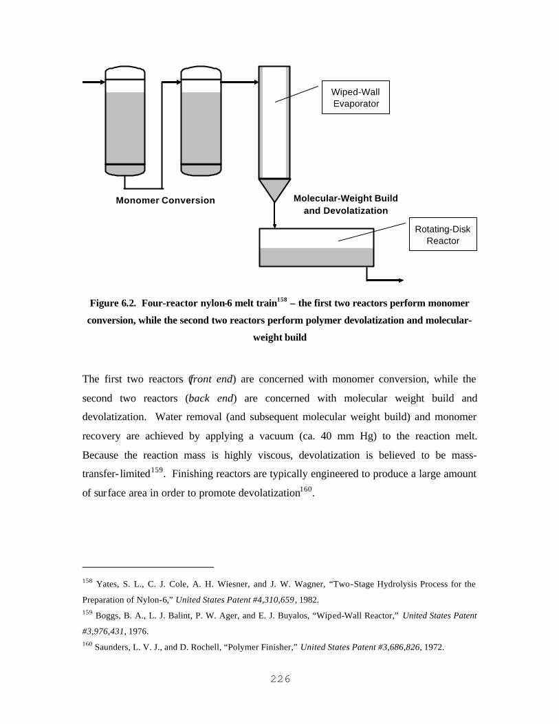
226
Monomer Conversion Molecular-Weight Build and Devolatization
Wiped-Wall Evaporator
Rotating-Disk Reactor
Figure 6.2. Four-reactor nylon-6 melt train158 – the first two reactors perform monomer
conversion, while the second two reactors perform polymer devolatization and molecular-
weight build
The first two reactors (front end) are concerned with monomer conversion, while the
second two reactors (back end) are concerned with molecular weight build and
devolatization. Water removal (and subsequent molecular weight build) and monomer
recovery are achieved by applying a vacuum (ca. 40 mm Hg) to the reaction melt.
Because the reaction mass is highly viscous, devolatization is believed to be mass-
transfer- limited159. Finishing reactors are typically engineered to produce a large amount
of surface area in order to promote devolatization160.
158 Yates, S. L., C. J. Cole, A. H. Wiesner, and J. W. Wagner, “Two-Stage Hydrolysis Process for the
Preparation of Nylon-6,” United States Patent #4,310,659 , 1982. 159 Boggs, B. A., L. J. Balint, P. W. Ager, and E. J. Buyalos, “Wiped-Wall Reactor,” United States Patent
#3,976,431, 1976. 160 Saunders, L. V. J., and D. Rochell, “Polymer Finisher,” United States Patent #3,686,826, 1972.
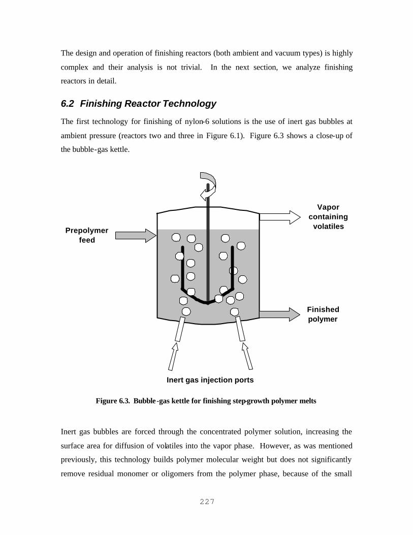
227
The design and operation of finishing reactors (both ambient and vacuum types) is highly
complex and their analysis is not trivial. In the next section, we analyze finishing
reactors in detail.
6.2 Finishing Reactor Technology
The first technology for finishing of nylon-6 solutions is the use of inert gas bubbles at
ambient pressure (reactors two and three in Figure 6.1). Figure 6.3 shows a close-up of
the bubble-gas kettle.
Inert gas injection ports
Prepolymerfeed
Finishedpolymer
Vapor containing
volatiles
Figure 6.3. Bubble-gas kettle for finishing step-growth polymer melts
Inert gas bubbles are forced through the concentrated polymer solution, increasing the
surface area for diffusion of volatiles into the vapor phase. However, as was mentioned
previously, this technology builds polymer molecular weight but does not significantly
remove residual monomer or oligomers from the polymer phase, because of the small
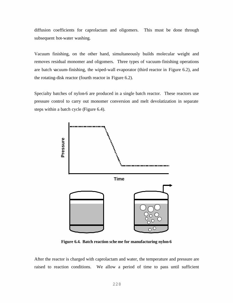
228
diffusion coefficients for caprolactam and oligomers. This must be done through
subsequent hot-water washing.
Vacuum finishing, on the other hand, simultaneously builds molecular weight and
removes residual monomer and oligomers. Three types of vacuum-finishing operations
are batch vacuum-finishing, the wiped-wall evaporator (third reactor in Figure 6.2), and
the rotating-disk reactor (fourth reactor in Figure 6.2).
Specialty batches of nylon-6 are produced in a single batch reactor. These reactors use
pressure control to carry out monomer conversion and melt devolatization in separate
steps within a batch cycle (Figure 6.4).
Pre
ssu
re
Time
Figure 6.4. Batch reaction sche me for manufacturing nylon-6
After the reactor is charged with caprolactam and water, the temperature and pressure are
raised to reaction conditions. We allow a period of time to pass until sufficient

229
conversion is achieved. We then ramp the pressure down to devolatilize the melt and
build polymer molecular weight. The vacuum causes boiling of the volatile species.
This example of mass-transfer- limited devolatization shows at least two avenues for the
escape of volatile species from the viscous polymer melt:
• Diffusion through the interfacial surface area between the liquid pool and vapor
head space
• Kinetically- limited phase transition from liquid to vapor (i.e., boiling)
The second example of a vacuum-finishing unit is the thin-film evaporator. It can be a
vertically-oriented vessel that wipes a thin polymer film on the inside wall of the
reactor161. Figure 6.5 illustrates the geometric configuration of this reactor.
161 Yates, S. L., C. J. Cole, A. H. Wiesner, and J. W. Wagner, “Two-Stage Hydrolysis Process for the
Preparation of Nylon-6,” United States Patent #4,310,659 , 1982.
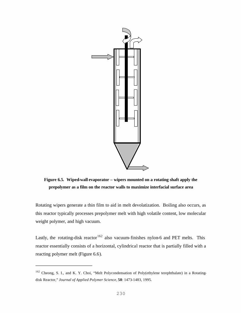
230
Figure 6.5. Wiped-wall evaporator – wipers mounted on a rotating shaft apply the
prepolymer as a film on the reactor walls to maximize interfacial surface area
Rotating wipers generate a thin film to aid in melt devolatization. Boiling also occurs, as
this reactor typically processes prepolymer melt with high volatile content, low molecular
weight polymer, and high vacuum.
Lastly, the rotating-disk reactor162 also vacuum-finishes nylon-6 and PET melts. This
reactor essentially consists of a horizontal, cylindrical reactor that is partially filled with a
reacting polymer melt (Figure 6.6).
162 Cheong, S. I., and K. Y. Choi, “Melt Polycondensation of Poly(ethylene terephthalate) in a Rotating-
disk Reactor,” Journal of Applied Polymer Science, 58: 1473-1483, 1995.
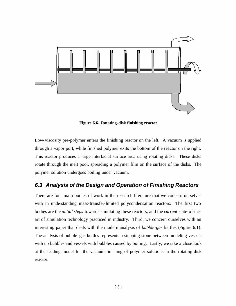
231
Figure 6.6. Rotating-disk finishing reactor
Low-viscosity pre-polymer enters the finishing reactor on the left. A vacuum is applied
through a vapor port, while finished polymer exits the bottom of the reactor on the right.
This reactor produces a large interfacial surface area using rotating disks. These disks
rotate through the melt pool, spreading a polymer film on the surface of the disks. The
polymer solution undergoes boiling under vacuum.
6.3 Analysis of the Design and Operation of Finishing Reactors
There are four main bodies of work in the research literature that we concern ourselves
with in understanding mass-transfer-limited polycondensation reactors. The first two
bodies are the initial steps towards simulating these reactors, and the current state-of-the-
art of simulation technology practiced in industry. Third, we concern ourselves with an
interesting paper that deals with the modern analysis of bubble-gas kettles (Figure 6.1).
The analysis of bubble-gas kettles represents a stepping stone between modeling vessels
with no bubbles and vessels with bubbles caused by boiling. Lastly, we take a close look
at the leading model for the vacuum-finishing of polymer solutions in the rotating-disk
reactor.

232
6.3.1 Initial Steps towards Understanding Finishing Reactors
Several papers illustrate the initial style of simulating mass-transfer- limited finishing
reactors. These papers include studies by Ault and Mellichamp 163, Amon and Denson164,
Ravindranath and Mashelker165, Gupta et al. 166, and Ahn167.
Their strategy consists of combining diffusion equations with reaction kinetics equations
to simulate finishing reactors. Figure 6.7 illustrates this approach applied to the analysis
of a wiped-wall reactor.
163 Ault, J. W., and D. A. Mellichamp, “A Diffusion and Reaction Model for Simple Polycondensation,”
Chemical Engineering Science, 27: 1441-1448, 1972; Ault, J. W., and D. A. Mellichamp, “Complex Linear
Polycondensation. II. Polymerization Rate Enhancement in Thick Film Reactors,” Chemical Engineering
Science, 27: 2233-2242, 1972 164 Amon, M., and C. D. Denson, “Simplified Analysis of the Performance of Wiped-Film
Polycondensation Reactors,” Industrial and Engineering Chemistry Fundamentals, 19: 415-420, 1980. 165 Ravindranath, K., and R. A. Mashelkar, “Modeling of Poly(Ethylene Terephthalate) Reactors: 6. A
Continuous Process for Final Stages of Polycondensation,” Polymer Engineering and Science, 22: 628-636,
1982. 166 Gupta, S. K., A. K. Ghosh, S. K. Gupta, and A. Kumar, “Analysis of Wiped Film Reactors Using the
Orthogonal Collocation Technique,” Journal of Applied Polymer Science, 29: 3217-3230, 1984. 167 Ahn, Y. C., “Effects of Diffusional Water Removal and Heat Transfer in Nylon-6 Reactors,” Polymer
Engineering and Science, 37: 484-493, 1997.

233
2
Diffusion
ii i
DCC
Dt= ∇D
Polymer Film Reactor
Wall
[ ]
Chemical Reaction
ii j k
dCk C C
dt = + …
Figure 6.7. Initial approach for modeling thin-film finishing re actors
Ci is the concentration of diffusing species i (mol/m3), iD is the diffusion coefficient of
species i, D/Dt is the substantial derivative with respect to time, ∇ is the gradient
operator, and ki is the rate constant for reaction i.
Some type of diffusion equation dictates the mass-transfer- limited volatization of small
molecules from the polymer melt. Both rigorous diffusion equations as well as simpler
penetration/film-type theories168 have been applied to analyze mass transfer. Reaction
kinetics are typically handled using standard reaction schemes, such as the one by Arai et
al.169 for nylon-6 polymerization.
168 Higbie, R., “The Rate of Absorption of a Pure Gas Into a Still Liquid During Short Periods of
Exposure,” Transactions of the American Institute of Chemical Engineers,” 31: 365-389, 1935; Whitman,
W. G., “Preliminary Experimental Confirmation of the Two-Film Theory of Gas Absorption,” Chemical
and Metallurgical Engineering, 29: 146-148, 1923. 169 Arai, Y., K. Tai, H. Teranishi, and T. Tagawa, “Kinetics of Hydrolytic Polymerization of ε-
Caprolactam: 3. Formation of Cyclic Dimer,” Polymer, 22: 273-277, 1981.
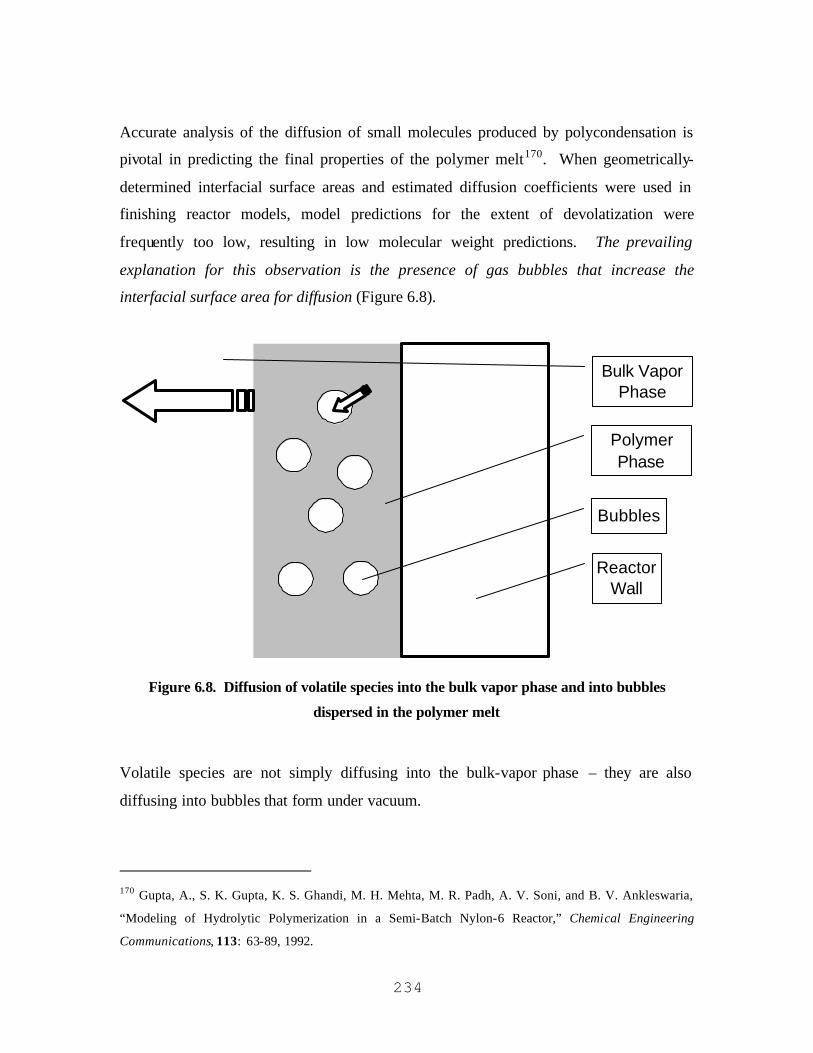
234
Accurate analysis of the diffusion of small molecules produced by polycondensation is
pivotal in predicting the final properties of the polymer melt170. When geometrically-
determined interfacial surface areas and estimated diffusion coefficients were used in
finishing reactor models, model predictions for the extent of devolatization were
frequently too low, resulting in low molecular weight predictions. The prevailing
explanation for this observation is the presence of gas bubbles that increase the
interfacial surface area for diffusion (Figure 6.8).
Bubbles
Polymer Phase
Reactor Wall
Bulk Vapor Phase
Figure 6.8. Diffusion of volatile species into the bulk vapor phase and into bubbles
dispersed in the polymer melt
Volatile species are not simply diffusing into the bulk-vapor phase – they are also
diffusing into bubbles that form under vacuum.
170 Gupta, A., S. K. Gupta, K. S. Ghandi, M. H. Mehta, M. R. Padh, A. V. Soni, and B. V. Ankleswaria,
“Modeling of Hydrolytic Polymerization in a Semi-Batch Nylon-6 Reactor,” Chemical Engineering
Communications, 113: 63-89, 1992.

235
The traditional approach to solving this problem is to simply leave the interfacial surface
area as an adjustable parameter and regressing a value to match actual reactor data171.
This fact reflects the empirical nature of finishing-reactor modeling, and the next section
shows how we currently model these processes in industry.
6.3.2 Current Modeling Approach for Industrial Finishing Reactors
The current modeling approach used in industrial process simulation of finishing reactors
is the single-parameter model for a general mass-transfer-limited reactor172. This model
is an elegant combination of simplicity, ease of application, and range of applicability. It
characterizes mass-transfer- limited devolatization using the penetration theory of
devolatization:
( ),, , , *
i LL i i L i L
dCk a C C
dt= − (6.1)
The change in the concentration of species i, ,i LC , in the liquid phase with respect to time
is a function of the product of the mass-transfer coefficient kL,ia and the liquid-phase
concentration gradient173. The gradient is the difference between the bulk-liquid
concentration, ,i LC , and the interfacial liquid-phase concentration in equilibrium with the
vapor phase , *i LC (Figure 6.9).
171 Laubriet, C., B. LeCorre, and K. Y. Choi, “Two-Phase Model for Continuous Final Stage Melt
Polycondensation of Poly(Ethylene Terephthalate). I. Steady-State Analysis,” Industrial and Engineering
Chemistry Research, 30: 2-12, 1991. 172 Laubriet, C., B. LeCorre, and K. Y. Choi, “Two-Phase Model for Continuous Final Stage Melt
Polycondensation of Poly(Ethylene Terephthalate). I. Steady-State Analysis,” Industrial and Engineering
Chemistry Research, 30: 2-12, 1991. 173 We typically assume that the vapor-phase film resistance to mass transfer is negligible compared with
the melt-phase film resistance

236
Co
nce
ntr
atio
n
Liquid Phase
VaporPhase
,i LC
, *i LC
Figure 6.9. Concentration profile vs. distance in a devolatizing slab of polymer solution
Based on the penetration theory for interfacial mass transfer, we may write the mass-
transfer coefficient ,L ik a in terms of the diffusion coefficient for species i, iD , the contact
time tc, and the specific interfacial surface area of contact a:
, 2L ic
k a atπ
= iD (6.2)
We determine the mass-transfer coefficient by regressing real reactor performance data
(e.g., amount of a specific component devolatized, molecular weight of the finished
polymer, etc.). This model is general in tha t it can accommodate any finishing reactor
configuration that involves liquid-vapor contacting. It is easy to use in that only one
parameter needs to be regressed, kLa. However, the model fails to characterize the
variation of the mass-transfer coefficient with feed composition and polymer molecular
weight, reactor temperature and pressure, and specifics regarding the operation of reactor
internals. This weakness severely limits our ability to learn about one type of
devolatization technology and then subsequently apply this knowledge to analyze a new
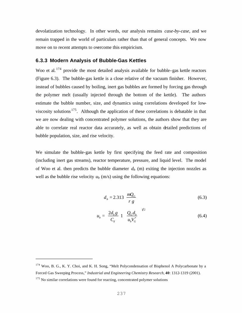
237
devolatization technology. In other words, our analysis remains case-by-case, and we
remain trapped in the world of particulars rather than that of general concepts. We now
move on to recent attempts to overcome this empiricism.
6.3.3 Modern Analysis of Bubble-Gas Kettles
Woo et al.174 provide the most detailed analysis available for bubble-gas kettle reactors
(Figure 6.3). The bubble-gas kettle is a close relative of the vacuum finisher. However,
instead of bubbles caused by boiling, inert gas bubbles are formed by forcing gas through
the polymer melt (usually injected through the bottom of the kettle). The authors
estimate the bubble number, size, and dynamics using correlations developed for low-
viscosity solutions 175. Although the application of these correlations is debatable in that
we are now dealing with concentrated polymer solutions, the authors show that they are
able to correlate real reactor data accurately, as well as obtain detailed predictions of
bubble population, size, and rise velocity.
We simulate the bubble-gas kettle by first specifying the feed rate and composition
(including inert gas streams), reactor temperature, pressure, and liquid level. The model
of Woo et al. then predicts the bubble diameter db (m) exiting the injection nozzles as
well as the bubble rise velocity ub (m/s) using the following equations:
2.313 Gb
Qd
gµρ
=
(6.3)
1 2
*
21b G b
bd b G
d g Q du
C u V
= +
(6.4)
174 Woo, B. G., K. Y. Choi, and K. H. Song, “Melt Polycondensation of Bisphenol A Polycarbonate by a
Forced Gas Sweeping Process,” Industrial and Engineering Chemistry Research, 40: 1312-1319 (2001). 175 No similar correlations were found for reacting, concentrated polymer solutions

238
µ is the solution viscosity (Pa s), QG is the volumetric flow rate of the gas (m3/s), ? is the
melt density (kg/m3), and g is the gravitational acceleration constant. Cd is the drag
coefficient (= 16/Re + 1) and *GV is the volume of a bubble (m3).
We compute the average residence time of the bubbles in the polymer solution tc (s) and
number of bubbles in solution Nb below:
( )1L G
cb R
Vt
u Sε+
= (6.5)
*G
bG
QN
Vθ
= (6.6)
VL is the polymer solution volume (m3), εG is the fractional gas holdup (volumetric basis),
ub is the bubble rise velocity (m/s), and SR is the cross-sectional area of the reactor (m2).
QG is the gas volumetric flow rate (m3/s) and *GV is the volume of a bubble (m3). We
compute the fractional gas holdup using an empirical correlation:
( )0.6342 0.50.239 10G b Ru Dε − −= × (6.7)
With detailed predictions for key quantities of bubble dynamics, we can compute the
mass-transfer coefficient ,L ik a (1/s) in Eq. (6.2):
*
, 2 b GL i
c L
N Sk a
t Vπ
=
iD (6.8)
iD is the diffusion coefficient for species i (m2/s), tc is the vapor- liquid average contact
time (s), Nb is the number of bubbles in solution, *GS is the interfacial surface area per
bubble (m2/bubble), and VL is the volume of polymer solution in the reactor (m3).

239
Once we obtain the mass-transfer coefficient, we are able to use the one-parameter
finishing reactor model, Eq. (6.1), to simulate the devolatization within the bubble-gas
kettle.
Again, although the range of applicability of these correlations is exceeded in
concentrated polymer solutions, Woo et al. 176 manage to successfully correlate molecular
weight build as a function of reaction time at varying reaction temperatures and gas flow
rates. However, they treat the diffusivity as an adjustable parameter because no value
was available in the literature.
6.3.4 Modern Analysis of Rotating-Disk Reactors
The most realistic model for rotating-disk reactors is the model of Cheong and Choi177.
They investigate the batch polymerization of poly(ethylene terephthalate) in lab-scale
rotating-disk reactor under vacuum. Cheong and Choi conceptualize the rotating-disk
reactor by splitting it into sections, with each rotating-disk and adjacent reactor space
comprising one compartment. The polymer on the disk (film phase) is modeled as a two-
phase plug-flow reactor (PFR), while the bulk polymer phase in each compartment is
modeled as a two-phase continuous-stirred-tank reactor (CSTR). Figure 6.10 shows a
diagram of their compartmental modeling methodology.
176 Woo, B. G., K. Y. Choi, and K. H. Song, “Melt Polycondensation of Bisphenol A Polycarbonate by a
Forced Gas Sweeping Process,” Industrial and Engineering Chemistry Research, 40: 1312-1319 (2001). 177 Cheong, S. I., and K. Y. Choi, “Melt Polycondensation of Poly(ethylene terephthalate) in a Rotating
Disk Reactor,” Journal of Applied Polymer Science, 58, pp. 1473-1483 (1995).

240
Film phase(PFR)
Bulk phase(CSTR)
Film phase
Bulk phase
Idealization
Compartment in Rotating-Disk Reactor
Figure 6.10. Compartmental modeling strategy for the rotating-disk reactor178
The amount of polymer taken up by the disks is estimated based on experimental results.
Besides the compartmental modeling strategy, this model is similar to the study of Woo
et al.179 in that it attempts to connect reactor operating variables, such as disk rotation
speed, to the mass-transfer coefficient in Eq. (6.1). This model therefore becomes useful
for determining the effect of disk spacing and rotation speed on devolatization
performance. It is also useful for examining the effects of temperature and pressure on
diffusional mass transfer and reaction. However, this approach suffers from the same
inherent empiricism of the one-parameter model of Laubriet et al. 180 – the mass-transfer
coefficients must be regressed from reactor data.
178 Cheong, S. I., and K. Y. Choi, “Melt Polycondensation of Poly(ethylene terephthalate) in a Rotating
Disk Reactor,” Journal of Applied Polymer Science, 58, pp. 1473-1483 (1995). 179 Woo, B. G., K. Y. Choi, and K. H. Song, “Melt Polycondensation of Bisphenol A Polycarbonate by a
Forced Gas Sweeping Process,” Industrial and Engineering Chemistry Research, 40: 1312-1319 (2001). 180 Laubriet, C., B. LeCorre, and K. Y. Choi, “Two-Phase Model for Continuous Final Stage Melt
Polycondensation of Poly(Ethylene Terephthalate). I. Steady-State Analysis,” Industrial and Engineering
Chemistry Research, 30: 2-12, 1991.

241
6.3.5 Literature Review Summary
As we have seen, traditional chemical-engineering analysis (transport phenomena,
thermodynamics, and reaction kinetics) and modern process simulation techniques have
yielded reasonable approximations for finishing reactors that do not involve boiling.
However, analysis of boiling phenomena has always been carried out in the grossest
fashion possible: the additional interfacial surface area generated by the presence of
bubbles as well as the mass loss of volatiles are accounted for by regressing the mass-
transfer coefficients from actual reactor data. While this yields a reactor model that
describes the current reactor conditions, this may not furnish a robust model that can
accurately predict/extrapolate to conditions other than those under which the model was
developed and validated.
A fundamental model for vacuum devolatization in rotating-disk reactors, on the other
hand, is different. Ideally, it should allow us to make accurate predictions for all types of
vacuum finishers.
Additionally, Laubriet et al.’s and Cheong and Choi’s models appear to generate
considerable confusion as to the exact role of vacuum and increased surface area in step-
growth finishing reactors. With these models, diffusional mass transfer is the primary
route for volatile removal. This remains the case even when a vacuum is used and
boiling of the solution takes place. Cheong and Choi181 count the interfacial area
generated by the bubbles as simply an additional surface area in their penetration theory
correlation. This appears objectionable because they have implicitly assumed that the
bulk-vapor phase and the gas phase present in the bubble have equal compositions.
Furthermore, they give no mechanism for predicting how this additional surface area
varies with operating conditions, such as pressure. Lastly, this opens the door to
unknowing abuse of current theories by industrial practitioners – when diffusion
coefficients are known, the additional surface area must be equal for all diffusing species.
181 Cheong, S. I., and K. Y. Choi, “Melt Polycondensation of Poly(ethylene terephthalate) in a Rotating
Disk Reactor,” Journal of Applied Polymer Science, 58, pp. 1473-1483 (1995).

242
Oftentimes, mass-transfer coefficients are manipulated unboundedly to fit data, resulting
in absurdities such as unequal areas of mass-transfer for different species.
We do not believe that present models accurately reflect the underlying mechanisms of
devolatization under vacuum. Any bubble formed in a supersaturated liquid is most
likely at or near chemical equilibrium with its surroundings182. Therefore, there is no
concentration driving force for mass transfer. This means that the bubbles do not
contribute additional surface area for diffusional mass transfer – rather, they contribute to
devolatization simply through gross phase change (i.e., boiling) directly from liquid to
vapor.
Evidence to support this notion comes from the nylon-6 polymerization literature. When
nylon-6 is finished in a rotating-disk reactor (or any vacuum finisher), we are
simultaneously increasing the polymer molecular weight (through water removal) and
removing residual caprolactam monomer183. This produces a nylon-6 melt that is suitable
for direct spinning (caprolactam mass fraction ~ 0.01). Seavey184 has previously shown
that removal of caprolactam through diffusional mass transfer is most likely too slow to
be significantly enhanced by vacuum or by reasonable surface-area enhancement. The
batch-reactor simulations of Chapter 5 show that a change of pressure from atmospheric
to 50 mm Hg does almost nothing for caprolactam devolatization. However, if we
postulate that vacuum enhances the flashing of volatiles from the concentrated nylon-6
solution, then we begin to see how significant amounts of caprolactam can be removed in
a commercially-feasible process through a route other than diffusional mass transfer.
The low diffusion coefficient of caprolactam (order of 8E-10 m2/hr) also suggests another
interesting fact – that all commercial technologies for nylon-6 production employ either
182 Holden, B. S., and J. L. Katz, “The Homogeneous Nucleation of Bubbles in Superheated Binary Liquid
Mixtures,” AIChE Journal, 24, pp. 260-266 (1978). 183 Yates, S. L., C. J. Cole, A. H. Wiesner, and J. W. Wagner, “Two-Stage Hydrolysis Process for the
Preparation of Nylon-6,” United States Patent #4,310,659 (1982). 184 Chapter 5 of this dissertation, Sec. 5.6

243
hot-water leaching or vacuum. This is because a reasonable increase in interfacial
surface area (as in the case of the bubble-gas kettles) is still not enough to remove
caprolactam due to the low diffusion coefficient.
We also believe that Cheong and Choi’s model185 is presently too complex for the general
analysis of existing rotating-disk reactors. This shortcoming is a result of weaknesses of
our understanding of rotating-disk reactors rather than a direct weakness of the model
itself. In their study, they experimentally measure the amount of polymer solution
dragged up onto the disks, and use these results to separate the film and bulk liquid
phases. If these experimental measurements are not available, then we cannot apply their
model. Therefore, this level of complexity, i.e., separation of the film and bulk liquid
phases, must be postponed until some generally reliable method is developed that can
accurately predict the amount of polymer dragged onto the disks as a function of the
polymer-solution properties and disk design.
We prefer to use a simpler series of CSTR’s to model the entire reactor, since there is
most likely some degree of back-mixing taking place between the reactor compartments.
The CSTR’s- in-series model has been successfully used to model a similar reactor – the
gas-phase polypropylene process186. The polypropylene reactor is characterized by a
plug-flow polymer particle phase and a well-mixed vapor phase. We use penetration
theory to analyze diffusional mass transfer, as do Cheong and Choi – however, we use
bubble-nucleation theory in order to model the formation of bubbles (and subsequent
removal of volatiles caused by bubble nucleation), rather than correct the mass-transfer
coefficient empirically and otherwise ignore bubble nucleation.
185 Cheong, S. I., and K. Y. Choi, “Melt Polycondensation of Poly(ethylene terephthalate) in a Rotating
Disk Reactor,” Journal of Applied Polymer Science, 58, pp. 1473-1483 (1995). 186 Caracotsios, M., “Theoretical Modeling of Amoco’s Gas Phase Horizontal Stirred Bed Reactor for the
Manufacturing of Polypropylene Resins,” Chemical Engineering Science, 47, pp. 2591-2596 (1992).

244
6.4 Theoretical
Now that we have reviewed the literature on analyzing various step-growth finishing
reactors, let us turn towards developing an improved and consistent theory for vacuum
reactors.
These reactors are operated under vacuum, causing foaming within the polymer melt, and
resulting in the flashing of volatiles and their release into the vapor phase. So far, we are
in agreement with the general understanding found in the literature – for example, see
Gupta et al. 187
Now, let us make the following assumption for modeling devolatization: mass transfer
due to surface regeneration and bubble formation and release, operate
independently and in an additive manner. In other words:
, ,i idiffusion ibubbleE E E= + (6.9)
The total evaporation rate of a volatile species i Ei (mol/s) is the sum of the contribution
of diffusion through interfacial surface area (bulk melt and vapor phases) Ei,diffusion and the
contribution due to bubble nucleation and release into the bulk vapor phase Ei,bubble. We
have to make this assumption because there is no way to predict non- ideal interactions
between bubble formation and diffusion in a reactor as complicated as the one we treat
here. However, we may say definitively that if either of these mechanisms dominates,
then the effect of non- ideality is most likely negligible.
We now turn to predicting the amount of bubbling based on processing conditions.
187 Gupta, S. K., A. K. Ghosh, S. K. Gupta, and A. Kumar, “Analysis of Wiped Film Reactors Using the
Orthogonal Collocation Technique,” Journal of Applied Polymer Science, 29, pp. 3217-3230 (1984).

245
6.4.1 Mass Transfer due to Bubbling
Bubble nucleation from a liquid phase, or cavitation, can either be homogeneous or
heterogeneous in nature. Homogeneous nucleation arises in supersaturated solutions due
to random fluctuations among the liquid molecules, thus forming a liquid/vapor interface.
Heterogeneous nucleation, on the other hand, occurs at pre-existing interfaces between
the liquid and a solid substrate. Classical nucleation theory predicts that heterogeneous
nucleation is always kinetically favored over homogeneous nucleation188. Furthermore,
concerning polymer solutions, it is generally accepted that bubble nucleation occurs
primarily through the heterogeneous mechanism. See, for example, Biesenberger and
Lee189. Therefore, we will treat bubble nucleation in the finishing reactor as being
heterogeneous.
In 1975, Blander and Katz190 published a review of the theoretical and experimental
aspects of both modes of nucleation. They extend the classical homogeneous nucleation
theory to describe heterogeneous nucleation by analyzing the minimum work to generate
a vapor- liquid interface at a pre-existing liquid-solid interface. They compute the
nucleation rate of bubbles due to heterogeneous nucleation in a single fluid:
( )
1exp
V Li
BJ A
T P Pm
= − −
(6.10)
J is the nucleation rate of bubbles (#/m2-hr), mi is the molecular weight of the vaporizing
molecule i (kg/kmol), T is the system temperature (K), and P is pressure (Pa) inside the
bubble (subscript V) and in the liquid phase (subscript L). Figure 6.11 illustrates the
188 Liu, X. Y., “Heterogeneous Nucleation or Homogeneous Nucleation?,” Journal of Chemical Physics,
112, pp. 9949-9955 (2000). 189 Biesenberger, J. A., and S. T. Lee, “A Fundamental Study of Polymer Melt Devolatization. Part I. Some
Experiments on Foam-Enhanced Devolatization,” Polymer Engineering and Science, 26, pp. 982-987
(1986). 190 Blander, M., and J. L. Katz, “Bubble Nucleation in Liquids,” AIChE Journal, 21, pp. 833-846 (1975).

246
distinction between the pressures and how they relate to surface tension under mechanical
equilibrium.
Figure 6.11. Depiction of pressures inside and outside the bubble, and the force of surface
tension. The equation is the condition for mechanical equilibrium, with r being the bubble
radius.
A and B are constants that depend on liquid properties such as surface tension, liquid
density, and the contact angle of the bubble on the solid surface:
1 2
2 3 2A N S
mσ
π =
(6.11)
316
2B
kπσ
= (6.12)
N is the number density of the liquid, cosm θ= − where θ is the contact angle between
the bubble and the solid surface, S = (1 – m) / 2, and k is Boltzmann’s constant.
Although A and B have values defined by theory, we choose to treat them as free
parameters because of the severe inaccuracies that can result when using their theoretical

247
values – see, for example, Han and Han191 or Zeng and Oxtoby192. Inaccuracies range
from predicting no bubble nucleation in cases where bubbles actually do form, to
predicting nucleation rates that are 15 orders of magnitude in error.
We now extend Eq. (6.10) to describe mixtures. Holden and Katz193 do so for
homogeneous nucleation - we follow their procedure to arrive at the similar expression
quantifying the rate of heterogeneous bubble nucleation in a mixture containing multiple
volatile species:
( )2expi
i i V L
y BJ A
m T P P
= − −
∑ (6.13)
yi is now the vapor mole fraction of volatile species i in the bubble, mi is the molecular
weight of molecule i (kg/kmol), T is the system temperature (K), and P is pressure (Pa)
inside the bubble (subscript V) and in the liquid phase (subscript L). The summation is
over all volatile species.
Blander and Katz194 show how to estimate the term V LP P− . Since PV is the vapor
pressure inside the bubble at a pressure PL and the equilibrium vapor pressure Pe is
measured on the liquid surface, they prescribe the following Poynting correction to the
difference between the equilibrium vapor pressure and the liquid pressure PL:
191 Han, J. H., and C. D. Han, “Bubble Nucleation in Polymeric Liquids. II. Theoretical Considerations,”
Journal of Polymer Science: Part B: Polymer Physics, 28, pp. 743-761 (1990). 192 Zeng, X. C., and D. W. Oxtoby, “Gas-Liquid Nucleation in Lennard-Jones Fluids,” Journal of Chemical
Physics, 94, pp. 4472-4478 (1991). 193 Holden, B. S., and J. L. Katz, “The Homogeneous Nucleation of Bubbles in Superheated Binary Liquid
Mixtures,” AIChE Journal, 24, pp. 260-266 (1978). 194 Blander, M., and J. L. Katz, “Bubble Nucleation in Liquids,” AIChE Journal, 21, pp. 833-846 (1975).
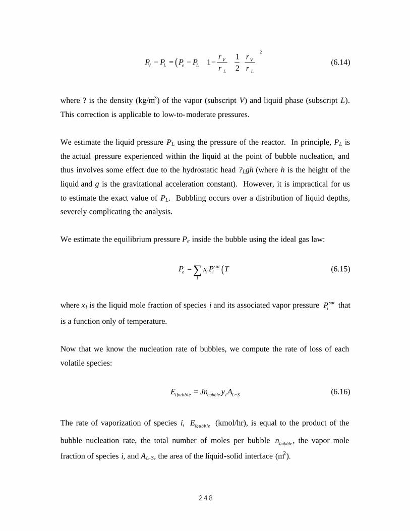
248
( )2
11
2V V
V L e LL L
P P P Pρ ρρ ρ
− = − − +
(6.14)
where ? is the density (kg/m3) of the vapor (subscript V) and liquid phase (subscript L).
This correction is applicable to low-to-moderate pressures.
We estimate the liquid pressure PL using the pressure of the reactor. In principle, PL is
the actual pressure experienced within the liquid at the point of bubble nucleation, and
thus involves some effect due to the hydrostatic head ?Lgh (where h is the height of the
liquid and g is the gravitational acceleration constant). However, it is impractical for us
to estimate the exact value of PL. Bubbling occurs over a distribution of liquid depths,
severely complicating the analysis.
We estimate the equilibrium pressure Pe inside the bubble using the ideal gas law:
( )sate i i
i
P x P T= ∑ (6.15)
where xi is the liquid mole fraction of species i and its associated vapor pressure satiP that
is a function only of temperature.
Now that we know the nucleation rate of bubbles, we compute the rate of loss of each
volatile species:
,ibubble bubble i L SE Jn y A −= (6.16)
The rate of vaporization of species i, ,ibubbleE (kmol/hr), is equal to the product of the
bubble nucleation rate, the total number of moles per bubble bubblen , the vapor mole
fraction of species i, and AL-S, the area of the liquid-solid interface (m2).

249
We now substitute Eq. (6.13) into Eq. (6.16) and lump the total number of moles per
bubble and the constant A into a single constant A’ to arrive at our final expression for the
rate of devolatization due to boiling:
( ), 2' expi
ibubble L S ii i V L
y BE A A y
m T P P−
= − −
∑ (6.17)
We use the ideal gas law relationship to estimate yi, the bubble vapor mole fraction for
species i which we assume to be in equilibrium with the liquid phase ( sati i i Ly x P P= ).
The important assumption inherent in Eq. (6.17) is that the bubble composition is in
thermodynamic equilibrium with the surrounding liquid. This has an interesting
consequence that will simplify our analysis of diffusional mass transfer and bubble
formation – that is, there is no mass transfer into the bubbles due to concentration
gradients.
An additional assumption that we make is that all bubbles that form eventually release
their contents into the vapor phase. This seems likely when agitation is applied to the
polymer solution. We do not need to treat bubble agglomeration or break-up explicitly –
whether or not bubbles break-up or agglomerate does not affect their ultimate future of
making it to the bulk-vapor/liquid interface and releasing their contents into the vapor
phase.
6.4.2 Mass Transfer due to Diffusion
Diffusion of volatiles takes place across the interface between the liquid and vapor
phases. We use the penetration theory195 to analyze diffusion.
195 Higbie, R., “The Rate of Absorption of a Pure Gas Into a Liquid Still During Short Periods of
Exposure,” Transactions of the Americal Institute of Chemical Engineers, 31, pp. 365-389 (1935).

250
6.4.2.1 Penetration Theory
Figure 6.12 shows the application of penetration theory to represent industrial unit
operations that involve agitation.
Bulk Liquid Phase(well-mixed)
Bulk Vapor Phase (well-mixed) Small region
of liquid near the vapor-
liquid interface
Movement of volatile species from the bulk liquid phase, through the interface, and into the bulk vapor phase
Figure 6.12. Penetration theory analysis of industrial-scale unit operations with agitation
We typically assume that a bulk, well-mixed liquid phase exists beneath a small
interfacial layer of fluid containing nearly all of the concentration gradient. Diffusion
mainly takes place through this small interfacial layer into the bulk vapor phase.
We compute the evaporation rate for species i out of the liquid phase Ei as follows:
( ), , int , , *idiffusion L i i L i LE k A C C= − (6.18)
,idiffusionE has units of kmol/hr. The mass-transfer coefficient for species i is ,L ik , which
has units of m/hr. ,i LC is the bulk liquid concentration of species i (mol/m3), while , *i LC
is the liquid interfacial concentration of i. Aint is the actual interfacial area (m2).

251
According to the penetration theory, we express ,L ik as twice the square root of the ratio
of the diffusion coefficient for species i, iD (m2/s), and the product of p and the contact
time, tc (s).
( ),
,
,2 i L
L ic
C Tk
tπ= iD
(6.19)
We assume that the diffusion coefficient is a function of the bulk-phase composition and
temperature – we use the function and parameters in Seavey196:
µ µ µ
µ* * *W CL NYLONW CL W C L NYLON W NYLON
W 0,W
( )exp
FH
V V V
V
ω ω ξ ω ξ
γ
+ + = −
D D (6.20)
2
0,Wm 3,010 J mol
4.38 7 exps
ERT
= − −
D (6.21)
µ µ µ
µ* * *W CL NYLONCL W W CL NYLON CL NYLON
CL 0,CL
( )exp
FH
V V V
V
ξ ω ω ω ξ
γ
+ + = −
D D (6.22)
2 2 2
20,CL 2
m m m2.47 13 2.74 10 4.77 08
s K s K sE T E T E
= − − + − + − −
D (6.23)
µ
( ) ( ) ( )* * *
W CL NYLONW W CL CL NYLON NYLON
W CL NYLON
ˆ ˆ ˆFH V V VVC T C T C T
B B Bω ω ω
γ
= + + + + +
(6.24)
Table 6.1 contains all of the free-volume parameters that accompany the above equations.
196 Chapter 5 of this dissertation, Sec. 5.5.2

252
Table 6.1. Summary of free-volume parameters for Eqs. (6.20), (6.22), and (6.24)
Species µ *iV (m3/kg) Bi (K) Ci (K)
Water (W) 9.93E-04 8.15E+02 -6.39E+01
Caprolactam (CL) 8.30E-04 6.43E+02 -2.27E+02
Nylon-6 (NYLON) 8.13E-04 4.77E+03 -9.18E+01
W-CLξ 5.52E-02
W-NYLONξ 8.54E-02
CL-Wξ 1.81E+01
CL-NYLONξ 1.55E+00
Additionally, we compute the interfacial surface concentrations by assuming that the
vapor is in equilibrium with the liquid interface – again, see Seavey197.
6.4.2.2 Estimating the Interfacial Surface Area and Renewal Time
We compute the interfacial surface area using geometric considerations. For a wiped-
wall reactor (see Figure 6.5), this interfacial surface area would be that of the falling film,
plus the surface area generated by the pool at the bottom of the reactor. The average
contact time for a fluid element is equal to the inverse of the product of the agitator
rotation speed ω and the number of wiper blades Nblades:
1
cblades
tNω
= (6.25)
If a higher agitation rate is employed, then the average contact time will decrease. An
increase in the amount of wiper blades also generates a decrease in the average contact
time.
197 Chapter 5 of this dissertation, Sec. 5.3.1

253
The analysis of the rotating-disk reactor can become somewhat more complicated –
however, expressions for the average contact time and interfacial surface area are
available in the literature – consult Ravetkar and Kale 198. These expressions account for
the liquid level within the vessel:
22ctπ θπω−
= (6.26)
? here refers to an angle that is geometrically related to the liquid level. Figure 6.13
shows a cross section of the rotating disk reactor with the angle ? and its relation to the
liquid level.
Theta
Liquid Level
Figure 6.13. Cross-section of rotating disk reactor depicting the liquid level and the
subsequent angle theta that is formed
The interfacial area for a single disk as a function of ? is below:
( )2
int
2 sin 1 cos2
2 2 2A R
π θ θ θπ
π π− +
= + −
(6.27)
R is the radius of the disk.
198 Ravetkar, D. D., and D. D. Kale, “Gas Absorption into Non-Newtonian Fluids in Rotating Disk
Contactors,” Chemical Engineering Science, 36, pp. 399-403 (1981).

254
6.4.3 Reaction Kinetics
Arai et al.199 have presented the accepted standard regarding the chemistry and kinetics of
the hydrolytic polymerization of caprolactam. Their reaction mechanism includes the
ring opening of caprolactam (CL), polycondensation, polyaddition of caprolactam, ring
opening of cyclic dimer (CD), and the polyaddition of cyclic dimer. We also include
monofunctional acid/amine termination reactions. We assume that cyclohexylamine
(CHA) behaves like a polymeric amine end group and that acetic acid (AA) behaves like
a polymeric carboxylic acid end group.
Table 6.2 lists these seven equilibrium reactions.
Table 6.2. Nylon-6 polymerization reaction mechanisms
Reaction Name Equilibrium Reaction
Ring opening of
caprolactam
1
1
k
1k '
W CL P+ �
Polycondensation 2
2
k
n m n+mk '
P P P W+ +�
Polyaddition of
caprolactam
3
3
k
n n+1k '
CL P P+ �
Ring opening of
cyclic dimer
4
4
k
2k '
W CD P+ �
Polyaddition of cyclic
dimer
5
5
k
n n+2k '
CD P P+ �
Polyaddition of
caprolactam with
cyclohexylamine
3
3
k
1,T-CHAk '
CL CHA P+ �
Polycondensation 3
3
k
n n,T-CHAk '
P CHA P+ �
199 Arai, Y., K. Tai, H. Teranishi, and T. Tagawa, “Kinetics of Hydrolytic Polymerization of ε-
Caprolactam: 3. Formation of Cyclic Dimer,” Polymer, 22, pp. 273-277 (1981).

255
with cyclohexylamine
Polycondensation
with acetic acid
3
3
k
n n,T-AAk '
P AA P+ �
*P1 is aminocaproic acid, Pn is nylon-6 with a degree of polymerization n.
For sake of simplicity, we ignore the formation of cyclics higher than two and we also
ignore the ring-opening of cyclic dimer with cyclohexylamine.
We use Aspen Dynamics software (Aspen Technology, Cambridge, MA) to simulate this
reaction/diffusion process, although our methodology is equally applicable in any
comparable polymer simulation software. This software tool uses a segment approach
for simulating this reaction set; Table 6.3 shows the segment definitions.
Table 6.3. Segment definitions used for simulating nylon-6 polymerization
Segment Name Molecular Structure
Non-polymeric segments
Water (W) H2O
Caprolactam (CL) C6H11NO
Cyclic dimer (CD) C12H22N2O2
Cyclohexylamine (CHA) C6H13N
Acetic acid (AA) C2H4O2
Polymeric segments
Amino caproic acid (P1) C6H13NO2
Terminal amine group (T-NH2) C6H12NO
Terminal carboxylic acid group (T-
COOH) C6H12NO2
Bound nylon 6 group (B-ACA) C6H11NO
Terminal cyclohexylamine group (T-
CHA) C6H12N
Terminal acetic acid group (T-AA) C2H3O

256
We re-write the equilibrium reactions in terms of the segment definitions and also include
the reaction rate expressions in Table 6.4.
Table 6.4. Equilibrium reactions using segment approach
Equilibrium Reaction Reaction Rate
Ring-opening of Caprolactam (1
1
k
1k '
W CL P+ � )
1
1 1 1
k
k ' = k K
1
CL + W
P
�����⇀↽�����
[ ][ ][ ]
1 1
1 1'
R k CL W
k P
=
−
Polycondensation (2
2
k
n m n+mk '
P P P W+ +� )
2
2 2 2
k1 1 k '=k K
P + P
T-COOH:T-NH2 + W
������⇀↽������ [ ][ ][ ]
22 2 1
2 2'
R k P
k P W
=
−
2
2 2 2
k1 k '=k K
P + T-COOH
T-COOH:B-ACA + W
������⇀↽������
[ ][ ]
[ ][ ] [ ][ ] [ ]
3 2 1
2 '2
R k P T COOH
B ACAk W T COOH
B ACA T NH
= −
−− − − + −
2
2 2 2
k1 k '=k K
T-NH2 + P
T-NH2:B-ACA + W
������⇀↽������
[ ][ ]
[ ][ ] [ ][ ] [ ]
4 2 1
2
2
' 2
R k T NH P
B ACAk W T NH
B ACA T COOH
= −
−− − − + −
2
2 2 2
k
k '=k KT-NH2 + T-COOH
B-ACA:B-ACA + W
������⇀↽������
[ ][ ][ ][ ]
[ ][ ] [ ]
5 2
2
2
'
2
R k T NH T COOH
k W B ACA
B ACAB ACA T NH
= − −
− −
− − + −
Polyaddition of Caprolactam (3
3
k
n n+1k '
CL P P+ � )
3
3 3 3
k1 k '=k K
P + CL
T-NH2:T-COOH
�����⇀�↽������ [ ][ ][ ]
6 3 1
3 2'
R k P CL
k P
=
−
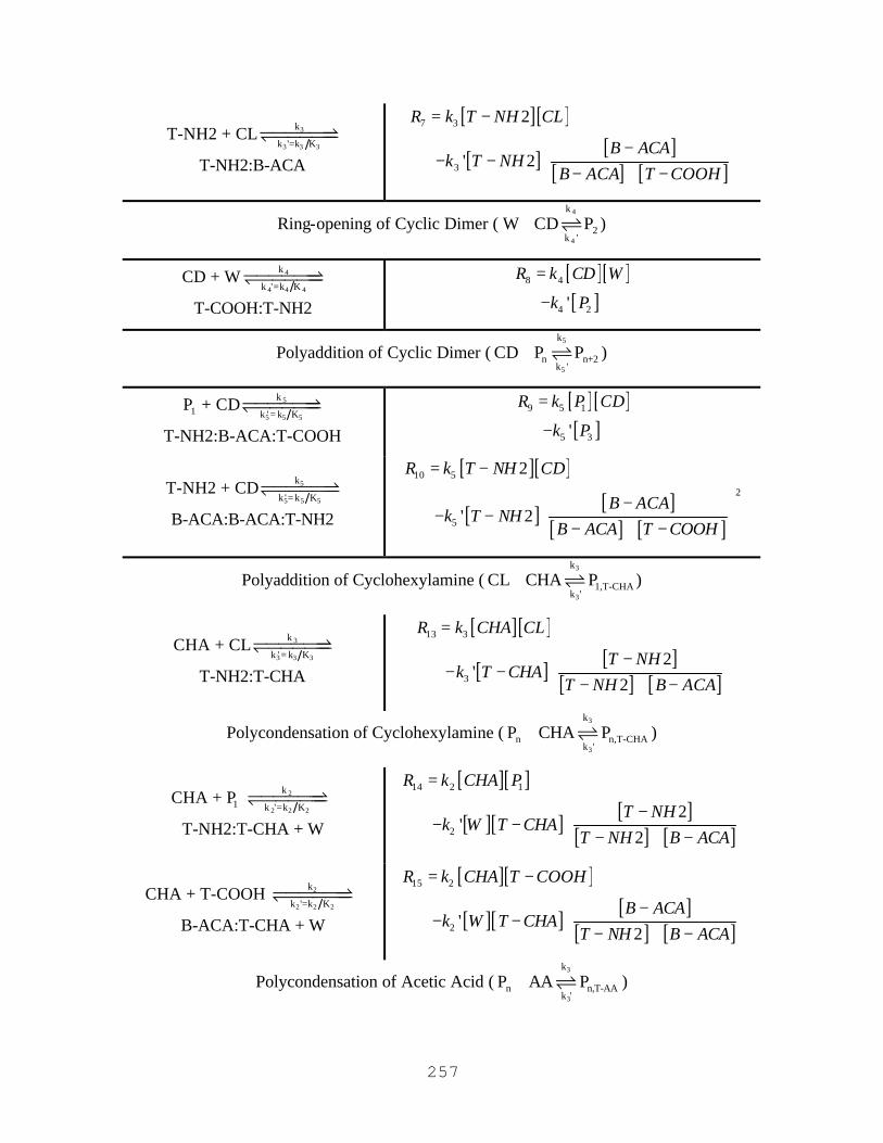
257
3
3 3 3
k
k '=k KT-NH2 + CL
T-NH2:B-ACA
�����⇀�↽������
[ ][ ]
[ ] [ ][ ] [ ]
7 3
3
2
' 2
R k T NH CL
B ACAk T NH
B ACA T COOH
= −
−− − − + −
Ring-opening of Cyclic Dimer (4
4
k
2k '
W CD P+ � )
4
4 4 4
k
k '=k KCD + W
T-COOH:T-NH2
������⇀↽������ [ ][ ][ ]
8 4
4 2'
R k CD W
k P
=
−
Polyaddition of Cyclic Dimer (5
5
k
n n+2k '
CD P P+ � )
5
5 5 5
k1 k ' = k K
P + CD
T-NH2:B-ACA:T-COOH
�����⇀�↽������ [ ][ ][ ]
9 5 1
5 3'
R k P CD
k P
=
−
5
5 5 5
k
k ' = k KT-NH2 + CD
B-ACA:B-ACA:T-NH2
�����⇀�↽������
[ ][ ]
[ ] [ ][ ] [ ]
10 5
2
5
2
' 2
R k T NH CD
B ACAk T NH
B ACA T COOH
= −
−− − − + −
Polyaddition of Cyclohexylamine (3
3
k
1,T-CHAk '
CL CHA P+ � )
3
3 3 3
k
k ' = k KCHA + CL
T-NH2:T-CHA
�����⇀�↽������
[ ][ ]
[ ] [ ][ ] [ ]
13 3
3
2'
2
R k CHA CL
T NHk T CHA
T NH B ACA
=
−− − − + −
Polycondensation of Cyclohexylamine (3
3
k
n n,T-CHAk '
P CHA P+ � )
2
2 2 2
k1 k '=k K
CHA + P
T-NH2:T-CHA + W
������⇀↽������
[ ][ ]
[ ][ ] [ ][ ] [ ]
14 2 1
2
2'
2
R k CHA P
T NHk W T CHA
T NH B ACA
=
−− − − + −
2
2 2 2
k
k '=k KCHA + T-COOH
B-ACA:T-CHA + W
������⇀↽������
[ ][ ]
[ ][ ] [ ][ ] [ ]
15 2
2 '2
R k CHA T COOH
B ACAk W T CHA
T NH B ACA
= −
−− − − + −
Polycondensation of Acetic Acid (3
3
k
n n,T-AAk '
P AA P+ � )

258
2
2 2 2
k1 k '=k K
P + AA
T-AA:T-COOH + W
������⇀↽������
[ ][ ]
[ ][ ] [ ][ ] [ ]
11 2 1
2 '
R k AA P
T COOHk W T AA
T COOH B ACA
=
−− − − + −
2
2 2 2
k
k '=k KT-NH2 + AA
B-ACA:T-AA + W
������⇀↽������
[ ][ ]
[ ][ ] [ ][ ] [ ]
12 2
2
2
'
R k AA T NH
B ACAk W T AA
T COOH B ACA
= −
−− − − + −
*A colon represents a covalent bond between polymer segments
The step-growth polymerization model approximates the concentrations of the terms [P2]
and [P3] (concentration of linear dimer and trimer) using the following approximations:
[ ] [ ] [ ][ ] [ ]2
22
T NHP T COOH
B ACA T NH
−= − − + −
(6.28)
[ ] [ ] [ ][ ] [ ]
[ ][ ] [ ]3
22 2
B ACA T NHP T COOH
B ACA T NH B ACA T NH
− −= − − + − − + −
(6.29)
These comprise the species balance terms in a liquid-only batch reaction. Table 6.5 gives
the species balance equations considering the reaction terms only.
Table 6.5. Species conservation equations for a liquid-only, batch reaction
Functional Group Time Rate of Change
W [ ]
( )2 3 4 5 11 12 14 15
1 8
d WR R R R R R R R
dtR R
= + + + + + + +
− +
CL [ ] ( )1 6 7 13
d CLR R R R
dt= − + + +
CD [ ] ( )8 9 10
d CDR R R
dt= − + +

259
AA [ ] ( )11 12
d AAR R
dt= − +
CHA [ ] ( )13 14 15
d CHAR R R
dt= − + +
P1
[ ]
( )
11
2 3 4 6 9 11 142
d PR
dtR R R R R R R
=
− + + + + + +
B-ACA [ ]3 4 5 7 9 10 12 152 2
d B ACAR R R R R R R R
dt
−= + + + + + + +
T-NH2 [ ]
( )2 6 8 9 13 14
5 12
2d T NHR R R R R R
dtR R
−= + + + + +
− +
T-COOH [ ]
( )2 6 8 9 11
5 15
d T COOHR R R R R
dtR R
−= + + + +
− +
T-AA [ ]11 12
d T AAR R
dt
−= +
T-CHA [ ]13 14 15
d T CHAR R R
dt
−= + +
6.5 Implementation
We model an industrial nylon-6 polymerization process using the mass-transfer concepts
outlined in Sec. 6.4. Particularly, we model the process depicted in Figure 6.2. Mass-
transfer- limited devolatization occurs in the wiped-wall evaporator and the rotating-disk
reactor.
Each of these reactors is plug-flow like. However, we use a series of CSTR’s to model
each vessel. About 8 CSTR’s behave identically to a PFR model. Furthermore, we have
chosen CSTR’s instead of PFR’s because implementing the mass-transfer equations (Eqs.
(6.17) and (6.18)) is easier in CSTR’s.

260
Figure 6.14 shows the simulation flow sheet.
MIXER
Figure 6.14. Simulation flow sheet for a continuous nylon-6 polymerization process
The kinetics of polymerization are described using proprietary rate constants – however
the numbers are similar to those appearing in Chapter 2, Table 2.5. The main difference
between the kinetics sets is that the proprietary set contains kinetics that describe the
effect of a polycondensation catalyst that is utilized in this process. Without this catalysis
effect, resulting molecular weights are too low because about one-third of the polymer
ends are terminated.
The custom modeling features in Aspen Dynamics allow us to include user-defined
equations (written in Visual BASIC) to compute the evaporation rate of each species
according to Eq. (6.9). The conventional dynamic CSTR model handles the reaction
terms in Table 6.4 and Table 6.5.
The procedure for developing this model appears below:
1. Establish the flow sheet, reaction kinetics, and physical properties – The reaction
set may include the reactions of Table 6.4 and the rate constants of Chapter 2,

261
Table 2.5. If thermodynamic equilibrium predictions are also being made, then
we should characterize the phase behavior of the reaction mixtures (Chapter 3).
2. Characterize diffusional-mass transfer for finishing reactors – Estimate the
diffusion coefficient using the techniques of Chapter 5 of this dissertation or use
an experimental value. Estimate the interfacial surface area available for
diffusion (Eq. (6.27) or some other similar expression). Estimate the average
contact time for diffusion (Eq. (6.26) or some other similar expression). Compute
the rate of diffusional-mass transfer using Eqs. (6.18) and (6.19).
3. Characterize bubbling mass transfer for finishing reactors – Compute the rate of
devolatization due to bubbling using Eq. (6.17). Regress the values of A’ and B
using two data points for the train. For our example, these data points are the
liquid concentrations of volatile species i coming out of the wiped-wall
evaporator and rotating-disk reactor.
4. Compute the total rate of devolatization for finishing reactors – using Eq. (6.9)
6.6 Model Performance and Validation
We attempt to reproduce known operating data for this train in a step-wise fashion. We
first attempt to describe the finishing reactors by considering diffusion only, and then we
invoke the description of bubbling in Eq. (6.17) to refine model predictions.
6.6.1 Using Diffusion to Model the Finishing Reactors
We now attempt to predict key characteristics of the nylon-6 polymer produced by the
train shown in Figure 6.2. We predict product characteristics for a production rate of
about 18,600 lb/hr. The three characteristics are FAV, extractables (mass %), and
polymer ends (amine and carboxyl, mmol/kg). Refer to Chapter 2, Sec. 2.5 for
procedures to compute these properties.
When we use diffusion only to model the two finishing reactors, we seriously under-
predict devolatization performance. Table 6.6 shows the process data and the model
predictions.

262
Table 6.6. Output variable predictions using only diffusional-mass transfer theory
Output Variable Data Model % Prediction Error
FAV 54.0 27.2 -50%
Extractables (%) 2.61 10.9 318%
Amine Ends (mmol/kg) 27.6 47.5 72%
Carboxyl Ends (mmol/kg) 20.5 40.7 98%
The FAV is under-predicted by 50% - this is an indication of too much water remaining
in the polymer phase. The extractables in the finished polymer melt is over-predicted by
318%. This indicates that caprolactam devolatization is seriously under-predicted.
Lastly, the amine and carboxyl ends are over-predicted by 72 and 98%, respectively.
That means that the predicted molecular weight of the polymer is too low, again
indicating that too much water remains in the polymer phase.
Table 6.7 shows the devolatization rates for water and caprolactam for the wiped-wall
evaporator and the rotating-disk reactor.
Table 6.7. Devolatization rates of finishing reactors considering diffusion as the sole
mechanism of devolatization
Water Devolatization Rate
(kmol/hr)
Caprolactam
Devolatization Rate
(kmol/hr)
Wiped-wall Evaporator 5.36E-01 6.64E-03
Rotating-disk Reactor 4.15E-02 5.08E-04
In general, the wiped-wall evaporator removes most of the volatiles from the nylon-6
solution, while the rotating-disk reactor finishes the polymer solution. This is because
the concentration of volatiles is higher in the wiped-wall reactor.

263
Figure 6.15 and Figure 6.16 show the computed diffusion coefficients for water and
caprolactam in each of the four CSTR’s for the wiped-wall evaporator and rotating-disk
reactor.
2.80E-04
3.00E-04
3.20E-04
3.40E-04
3.60E-04
3.80E-04
4.00E-04
CSTR-1 CSTR-2 CSTR-3 CSTR-4
Wat
er D
iffu
sio
n C
oef
ficie
nt (
m2 /h
r)
Wiped-Wall EvaporatorRotating-Disk Reactor
Figure 6.15. Diffusion coefficient of water in the wiped-wall evaporator and rotating-disk
reactor

264
0
5E-11
1E-10
1.5E-10
2E-10
2.5E-10
CSTR-1 CSTR-2 CSTR-3 CSTR-4
Cap
rola
ctam
Dif
fusi
on
Co
effi
cien
t (m
2 /hr)
Wiped-Wall EvaporatorRotating-Disk Reactor
Figure 6.16. Diffusion coefficient of caprolactam in the wiped-wall evaporator and rotating-
disk reactor
In Chapter 5, Table 5.12, we saw that the diffusion coefficients at 265 °C for water and
caprolactam are 4.21E-4 and 8.32E-10 m2/hr, respectively. Our finishing reactors are
operating at 255 °C – this is why the diffusion coefficients here are somewhat lower. We
predict the temperature dependence using the Dullian equation200. The diffusion
coefficients also vary along the length of each vessel. This variation is due to the change
in composition of the reaction mass, and we predict this variation using the Vrentas-Duda
free-volume theory201. The variation with respect to composition for the caprolactam
diffusion coefficient does not appear negligible – the diffusion coefficient has decreased
by an order of magnitude in the wiped-wall evaporator.
200 Dullien, F. A. L., “Predictive Equations for Self-Diffusion in Liquids: a Different Approach,” AIChE
Journal , 18, pp. 62-70 (1972). 201 Vrentas, J. S., and J. L. Duda, “Diffusion in Polymer-Solvent Systems. I. Reexamination of the Free-
Volume Theory,” Journal of Polymer Science, Polymer Physics Edition, 15, pp. 403-416 (1977).

265
Now, as we have seen in the literature review (Sec. 6.3), under-predicting devolatization
performance has been encountered before in the literature202. The proposed answer to
this problem from previous workers in this field (such as Cheong and Choi203), once
again, is that there exists additional, unaccounted-for surface area for interfacial mass
transfer in these reactors. This additional surface area arises from the presence of
microscopic bubbles. We therefore fit the extractables and molecular-weight data for the
train by multiplying the interfacial surface area terms by a number. The numbers that we
need are 8.7E3 for the wiped-wall evaporator and 2.5E5 for the rotating-disk reactor.
While these numbers are high, it is not physically impossible to realize them. We shall
demonstrate this below.
We may estimate the critical bubble radius using the classical force balance204:
2
cV L
rP P
σ=
− (6.30)
The bubble sizes in the rotating-disk reactor are on the order of 1E-6 m when using the
surface tension available for nylon-6 at 265 °C 205. About 1E17 bubbles need to be
present in the rotating-disk reactor to realize the observed multiplication factor.
However, due to the extremely small size of these bubbles, their volume only amounts to
about 1% of the liquid volume of the reactor. Thus, the observed multiplication factors
do not seem unreasonable.
202 Cheong, S. I., and K. Y. Choi, “Melt Polycondensation of Poly(ethylene terephthalate) in a Rotating
Disk Reactor,” Journal of Applied Polymer Science, 58, pp. 1473-1483 (1995). 203 Cheong, S. I., and K. Y. Choi, “Melt Polycondensation of Poly(ethylene terephthalate) in a Rotating
Disk Reactor,” Journal of Applied Polymer Science, 58, pp. 1473-1483 (1995). 204 Blander, M., and J. L. Katz, “Bubble Nucleation in Liquids,” AIChE Journal, 21, pp. 833-846 (1975). 205 Mehta, R. H., “Physical Constants of Various Polyamides,” in Polymer Handbook (4th ed.) , J. Brandrup,
E. H. Immergut, and E. A. Grulke, eds., Wiley, New York, p. V-124 (1999).

266
However, there is one objection which seems insurmountable when using this modeling
procedure. When modeling the diffusion of volatiles into the bubbles, we must know the
vapor-phase composition of the bubbles to compute the boundary condition for diffusion.
Strictly speaking, we may be in gross error if we say that the bubble-vapor-phase
composition is equal to the bulk-vapor-phase composition, as is done in Cheong and
Choi206 and Laubriet et al.207 To be rigorous, if we want to write penetration-theory
equations to describe diffusion into the bubbles, we must keep track of the bubble-vapor-
phase composition separately.
When one asks what the bubble vapor composition is, the immediate response is that it is
at or near equilibrium with the liquid phase. Once one admits to that, then it is seen that
the driving force for mass transfer vanishes, and the bubbles do not contribute to
diffusional mass-transfer at all. Therefore, it seems as though bubbles contribute to
devolatization only by nucleation itself – there is no subsequent diffusion of volatiles
from the liquid phase to the bubble phase.
In any case, it is reasonable to assume the following. Whether or not bubbles contribute
to diffusion or not, bubbles are believed to exist. Therefore, we must undertake the task
of fundamentally predicting bubble nucleation in order to make advancements in our
understanding of finishing-reactor performance. We believe that bubbles do not
contribute to diffusion; therefore, we limit ourselves to fundamentally modeling only the
devolatization rate through bubble nucleation. We have developed such a theory in Sec.
6.4.1, and we now apply it below.
206 Cheong, S. I., and K. Y. Choi, “Melt Polycondensation of Poly(ethylene terephthalate) in a Rotating
Disk Reactor,” Journal of Applied Polymer Science, 58, pp. 1473-1483 (1995). 207 Laubriet, C., B. LeCorre, and K. Y. Choi, “Two-Phase Model for Continuous Final Stage Melt
Polycondensation of Poly(Ethylene Terephthalate). I. Steady-State Analysis,” Industrial and Engineering
Chemistry Research, 30: 2-12, 1991.

267
6.6.2 Using Diffusion and Bubbling to Model the Finishing Reactors
We superimpose bubble nucleation onto diffusion via Eq. (6.9). We regress the two
parameters A’ and B for Eq. (6.17) using the caprolactam content of the exit streams for
the wiped-wall reactor and the rotating-disk reactor. The values are A’ = 0.273 kmol/hr-
m2 and B = 1.37E12 K-Pa2. We obtain the following improved predictions for key
polymer characteristics.
0
10
20
30
40
50
60
14000 15000 16000 17000 18000 19000
Production Rate (lb/hr)
Finisher Pressure (mm Hg, Data)Finisher Pressure (mm Hg, Model)FAV (Data)FAV (Model)Extractables (%, Data)Extractables (%, Model)Amine Ends (mmol/kg, Data)Amine Ends (mmol/kg, Model)Carboxyl Ends (mmol/kg, Data)Carboxyl Ends (mmol/kg, Model)
Figure 6.17. Key polymer characteristic as a function of production rate
The wiped-wall evaporator and rotating-disk reactor operate at essentially a constant
temperature over the production-rate range.
We see that the theory we have implemented to describe devolatization by both bubble
nucleation and diffusion can adequately describe the plant data for a wide range of
production rates. This result shows that there no longer remains the question whether the

268
bubble nucleation theory in Eq. (6.17) can be implemented accurately to describe real,
industrial processes.
Figure 6.17 also suggests that we are modeling the devolatization of water correctly,
since the polymer end-group-concentration predictions are quantitatively correct. We did
not use any water devolatization data to obtain the coefficients A’ and B. The water
devolatization predictions through bubbling are made using only caprolactam
devolatization data.
Table 6.8 shows the evaporation rates due to bubbling and diffusion for the wiped-wall
evaporator and the rotating-disk reactor for low and high production rate conditions.
Table 6.8. Devolatization rates for the wiped-wall evaporator and rotating-disk reactor –
bubbling mechanism vs. diffusion mechanism (numbers in parentheses are approximate
production rates)
Water Devolatization Rate
(kmol/hr)
Caprolactam Devolatization
Rate (kmol/hr)
Bubbling Diffusion Bubbling Diffusion
Wiped-wall
Evaporator
(15,000 lb/hr)
1.38E+00 4.00E-03 6.95E+00 7.32E-04
Rotating-Disk
Reactor
(15,000 lb/hr)
1.04E-01 3.95E-05 1.18E+00 6.79E-06
Wiped-wall
Evaporator
(18,600 lb/hr)
1.61E+00 5.06E-03 8.14E+00 1.17E-03
Rotating-Disk
Reactor 1.74E-01 4.91E-05 2.25E+00 9.02E-06

269
(18,600 lb/hr)
It is interesting to note that for the case of nylon-6, devolatization due to bubbling seems
to account for greater than 99% of the total devolatization. In other words, mass transfer
by diffusion plays a negligible role in this process. We may therefore adequately
describe this process using bubble nucleation theory alone.
As an aside, we may estimate the number of bubbles that are leaving each reactor. We
now do so for the 18,600 lb/hr case. We saw from the previous section that the
approximate size of the bubbles is 1E-6 m in radius. According to the ideal gas law, the
density of the bubble is 0.00121 kmol/m3. Therefore, the evaporator is removing about
1.92E+21 bubbles/hr and the finisher is removing about 4.76E+20 bubbles/hr. These
correspond to vapor flow rates of 8,030 and 2,000 m3/hr, respectively.
However, one question still remains, and that is, which mechanism better describes the
dependence of devolatization performance on temperature and pressure? Unfortunately,
our validation data do not contain any significant variation in reactor pressure, and
commercial processes for nylon-6 are notorious for producing a relatively uniform
product. If bubble nucleation is the primary mechanism for devolatization in nylon-6
vacuum reactors, then Eq. (6.17) should be able to better describe the dependence of
devolatization performance on reactor pressure and temperature. Seeing which equation
(Eq. (6.17) or Eq. (6.1)) better describes batch, vacuum reactor data would enable us to
see this relationship. This would allow us to make definitive statements about the
fundamental accuracy of proposed mechanisms.
One may now inquire about the choice between these two theories. Tentatively, the
performance of the empirical forms for bubble nucleation and penetration theory seems
equal. No distinction has been made as to the accuracy of these two theories. Therefore,
is there any reason why we should use one rather than the other?
270
The answer to this question is yes – these two theories differ in their ease of applicability
and number of parameters. In order to describe n apparent finishing reactors with m
volatile species, the number of equations that have to be written for each theory is m
times n. In our case, we have eight apparent finishing reactors (four CSTR’s for the
wiped-wall evaporator and four CSTR’s for the rotating-disk reactor) and we model the
devolatization of water and caprolactam. Therefore, for both bubble nucleation and
diffusion, we write 16 equations total.
However, the number of constants C has a different relationship. The number of
constants may or may not depend on the number of volatile species and the number of
real finishing reactors k (for this example, k = 2):
bubble-nucleation 2C = (6.31)
diffusionC km= (6.32)
We have assumed that the same mass-transfer coefficient applies to all sub-models of a
single, real finishing reactor.
The number of constants is important because it equals the number of data points needed
to uniquely determine the values for the constants. We see that the number of constants
needed to describe diffusion depends on both the number of components m and the
number of real finishing reactors k. However, bubble nucleation theory explicitly handles
removal of all volatile species at the same time, in a ratio dictated by phase equilibrium.
Therefore, we may say that bubble-nucleation theory is easier to implement and requires
fewer parameters and therefore less data to characterize. This means that when
appropriate (as the data seem to suggest for nylon-6 polymerization), using bubble
nucleation theory to model the loss of volatiles is more economical.
Eq. (6.31) is based on the assumption that the surface tension of the polymer solutions
processed in all mass-transfer- limited reactors is similar. Furthermore, it assumes that the
271
surfaces of the reactors are similar. If these assumptions do not apply, then Eq. (6.31)
becomes:
bubble-nucleation 2C k= (6.33)
In this case, we see that the number of constants is proportional to the number of mass-
transfer- limited reactors being described, but is not a function of the number of volatile
species being considered. This is important if we wish to model the devolatization of
additional species, such as aminocaproic acid and cyclic dimer. Accurate devolatization
analysis is important for analyzing the primary mode of failure in vacuum-melt trains:
entrainment and plugging of the vacuum lines.
There does exist a weakness of the current bubble nucleation theory – it does not predict
any rotation-rate dependence on devolatization performance. Industrial experience208 for
both PET and nylon-6 reactors suggest tha t devolatization rates linearly scale with
rotation rate:
iE ω∝ (6.34)
Penetration theory predicts that the evaporation rate scales with the rotation rate to the
one-half power (Eqs. (6.19) and (6.25)). To correct this, we simply change the power to
one instead of one-half.
We can employ a similar procedure to “patch” the bubble nucleation theory:
( ), 2' expi
ibubble L S ii i V L
y BE A A y
m T P Pω −
= − −
∑ (6.35)
208 David Tremblay, Aspen Technology, Cambridge, MA. Personal communication, 2003.
272
While this procedure is completely empirical and has no theoretical basis, it enables the
bubble nucleation theory to estimate the observed rotation-rate dependence.
When one searches for a possible theoretical explanation for the observed rotation-rate
dependence, one can arrive at two possibilities. One is that shear forces somehow lower
the activation energy barrier for bubble nucleation209. However, a quantitative
relationship for how this takes place is yet to be found. The second explanation is that
fluid elements become depleted of volatiles because of lack of sufficient agitation. For
example, a fluid element may remain on a rotating disk long enough to become depleted
of volatiles before being returned to the bulk melt pool. An increase in agitation rate
would mix these fluid elements faster, therefore reducing their average contact time.
However, pursuing this mode of explanation is quite burdensome, as one would have to
embark on the task of quantitatively predicting the amount of material being dragged up
onto disks.
6.7 Conclusions
In this study, we develop a model for vacuum-type finishing reactors. It explicitly
accounts for mass transfer of volatiles through two pathways – diffusional mass transfer
across the liquid-vapor interface and mass transfer caused by bubble nucleation and
eventual release into the vapor phase. This model represents an improvement over past
models in that it is the first reactor model in the literature to simultaneously consider
polymerization reactions, mass transfer through diffusion, and mass transfer through
boiling. Although it seems to accurately approximate the key features of very
complicated unit operations, the model remains tractable and can be implemented using
commercial software tools.
We demonstrate that the model can simulate a continuous reactor train that utilizes two
types of vacuum finishing reactors. We show that the observed devolatization
performance is unexplainable on the basis of diffusion alone. Large multiplication 209 Lee, S. T., “Shear Effects on Thermoplastic Foam Nucleation,” Polymer Engineering and Science, 33,
pp. 418-422 (1993).

273
factors must be used to account for additional surface area. We may object to these large
multiplication factors not because of their magnitude, but rather because it appears that
there exists no driving force for mass transfer into the bubbles.
Industrial practitioners now have three choices to model their vacuum finishing reactors:
the model of Laubriet210, the model of Cheong and Choi211, and our model. The models
of Laubriet and Cheong and Choi suffer from inherent empiricism in that their mass-
transfer parameters must always be fitted to reactor performance data. This sometimes
forces us into contradictions in those cases in which we know what the diffusion
coefficients are – we sometimes must assume that certain species enjoy more interfacial
surface area for diffusion or shorter average contact times. They also suffer in that they
do not separate and clarify the effects of boiling and diffusional mass transfer on total
devolatization – this can make it difficult to accurately estimate the effects of process
variables on boiling in concentrated polymer solutions.
Bubble-nucleation theory, on the other hand, does specifically account for boiling
behavior under vacuum. This makes it more fundamental. There are three consequences
of applying the fundamental theory of boiling. First, we have significantly decreased our
data requirements. Cheong and Choi fit the mass-transfer parameters to every
temperature/pressure condition they test – in our case, we would have to fit mass-transfer
parameters to both the water devolatization rate and the caprolactam devolatization rate.
When modeling boiling phenomena directly, fitting the bubble-nucleation parameters for
caprolactam devolatization automatically fixes the additional devolatization of water
through boiling. Second, when we start quantifying the behavior of bubbles, we march to
the eventuality of estimating how many bubbles there are and where they exist. This is
useful information for reactor design – consider the problems of estimating the amount of
210 Laubriet, C., B. LeCorre, and K. Y. Choi, “Two-Phase Model for Continuous Final Stage Melt
Polycondensation of Poly(Ethylene Terephthalate). I. Steady-State Analysis,” Industrial and Engineering
Chemistry Research, 30: 2-12, 1991. 211 Cheong, S. I., and K. Y. Choi, “Melt Polycondensation of Poly(ethylene terephthalate) in a Rotating
Disk Reactor,” Journal of Applied Polymer Science, 58, pp. 1473-1483 (1995).
274
work needed to rotate the disks and also the heat-transfer rates, for instance. And third,
we contribute towards the development of finishing reactors in general, and work
towards the eventuality in which we will be able predict the behavior of similar vacuum
finishers instead of treating each on a case-by-case basis.

275
6.8 Nomenclature
Symbol Description Units
intA Interfacial area m2
Ai0 Pre-exponential factor for uncatalyzed
forward reaction i kg/mol-hr
Aic Pre-exponential factor for catalyzed
forward reaction i kg/mol-hr
,i LC Concentration of species i in the bulk liquid phase kmol/m3
, *i LC Concentration of species i at the liquid-side interface kmol/m3
iD Diffusion coefficient of species i m2/hr
0,iD Pre-exponential diffusion coefficient for species i m2/hr
Ei Evaporation rate for species i kmol/hr
,ibubbleE rate of species i through bubble nucleation kmol/hr
,idiffusionE Evaporation rate of species i through diffusion kmol/hr
Ei0 Activation energy for uncatalyzed
forward reaction i J/mol
Eic Activation energy for catalyzed
forward reaction i J/mol
FAV Formic-acid viscosity Unitless
iH∆ Enthalpy of reaction i J/mol
J Nucleation rate of bubbles #/m2-hr
Ki Equilibrium constant for reaction i Unitless
ki Forward rate constant for reaction i kg/mol-hr
ki’ Reverse rate constant for reaction i kg/mol-hr
,L ik a Mass-transfer coefficient for species i 1/hr
mi Molecular weight of species i kg/kmol
nM Number-average molecular weight kg/mol
P Pressure Pa
276
satiP Vapor pressure of species i Pa
Px Polymer chain with degree of polymerization x N. A.
Px,y Polymer chain with degree of polymerization x and
termination condition y N. A.
R Radius of rotating disk m
Ri Rate equation for reaction i N. A.
iS∆ entropy of reaction i J/mol-K
T Temperature K
ct Contact time hr
,c iV Critical molar volume of species i m3/mol
0iV Specific volume of species i m3/kg
LV Volume of the liquid phase m3
µFHV Specific hole free volume for the mixture m3/kg
µ *iV Specific hole free volume for species i m3/kg
xi Liquid mole fraction of species i Unitless
nx Number-average degree of polymerization Unitless
yi Vapor mole fraction of species i Unitless
γ Overlap factor for the mixture Unitless
θ Angle related to liquid level in a horizontal cylinder Radians
i jξ Ratio of the molar volumes of the jumping units for
species i and j Unitless
σ Surface tension N/m
iω Weight fraction of species i Unitless

277
7 Conclusions and Future Work
This dissertation provides an in-depth analysis of all major aspects of building simulation
models for nylon-6 processes. We present new models for nylon-6 phase equilibrium,
diffusion coefficients, and devolatization of nylon-6 under vacuum conditions. These
advances allow industrial practitioners to accurately simulate most major nylon-6
production technologies.
There are additional aspects of nylon-6 polymerizations that need further investigation.
These are the areas of heat transfer and mass-transfer- limited devolatization.
7.1 Heat Transfer
Heat transfer is important in the design of front-end reactors. We typically operate these
reactors using a temperature profile. This profile is governed by Dowtherm loops around
major sections of the reactor. In order to investigate temperature options for cyclic dimer
mitigation, we must know which temperature profiles are accessible. To do this, we must
be able to accurately compute heats of reaction and heat-transfer through the vessel walls.
No fundamental, experimental studies have appeared in the literature regarding heats of
reaction of nylon-6 polymerization mixtures. It is interesting to note that enthalpies of
reaction are regressed from reaction data alone (concentrations vs. time) – they do not
come directly from heat of reaction data. Furthermore, because DIPPR data banks enable
us to compute the enthalpies of reactants and products, we may compute the enthalpy of
reaction directly. Because the enthalpies of reaction have not been physically verified,
they remain tentative.
7.2 Mass-Transfer-Limited Devolatization
The theories in Chapter 6 have received partial validation. Perhaps the most
comprehensive test for vacuum-devolatization theories is the simulation of the batch
reactor. This reactor utilizes a pressure profile rather than a single pressure – therefore, it

278
is a valuable test case for any theory that purports to model the pressure dependence of
devolatization. Experimental time-profile composition data in a batch reactor would be
useful here.
In addition, experimental work would be valuable in clarifying the devolatization
mechanism. Experiments that characterize the bubble population and size, and also the
devolatization rate will show whether diffusion into the bubbles plays a significant role.
Our devolatization analysis assumes that no diffusion into bubbles occurs.
Another avenue for future work is accurately modeling the RPM dependence of
devolatization – this is especially important for higher viscosity melts, such as PET.
Developing a general expression for computing the hold up on disks is important, though
difficult because such an expression would no doubt depend on the disk design. Such an
expression would allow one to test the hypothesis that RPM limitations are caused by
rapid depletion of volatiles of the held-up solution.
Another hypothesis for the RPM dependence has been suggested by David Tremblay212.
He suggests that RPM dependence may be linked to the rate- limiting dragging of bubbles
out of the bulk solution and to the surface where they can burst and release their contents
to the bulk vapor phase. Flow-field modeling may be useful here, mainly for visualizing
bubble flow.
Up until now, we have focused on process design. Modern analysis of polymer processes
now stress product design rather than process design. Product design for polymers
requires an in-depth knowledge of polymer properties and their origin. This field
concerns the molecular, physical chemistry of polymers. Much work remains to be done
in this field. Interesting research topics include visualizing the development of
morphology in polymerization reactors and the subsequent impact on processing
properties, such as rheology. Understanding processes at this level will no doubt require
212 David Tremblay, Aspen Technology, Cambridge, MA. Personal communication (2003).

279
multi-scale modeling efforts that span a range of length scales – fundamental
relationships between molecular phenomena and macroscopic properties are of interest
here.
280
Vita
Kevin Christopher Seavey was born second of identical twins in Downey, California on
March 4, 1975. Shortly thereafter, he and his family moved to Maryland. During his
stay at Old Mill Senior High School (Millersville, MD), he found that he was competitive
in wrestling, co-captaining his team to a fifth straight state championship and was the
state runner-up in the 130 lb. weight class. Furthermore, during high school, he attained
the rank of Eagle Scout in the Boy Scouts of America.
After graduating from high school in 1993, he attended the Johns Hopkins University
(Baltimore, MD) to study chemical engineering. He graduated in the spring of 1997 with
a Bachelor of Science in Chemical Engineering. In the spring of 1998, he began graduate
study in forest products under the direction of Wolfgang Glasser at Virginia Polytechnic
Institute and State University (VPI&SU, Blacksburg, VA). He completed the
requirements for a Master of Science in September of 1999. He then entered the
chemical engineering curriculum at VPI&SU to study computer-aided process design
under Y. A. Liu. He completed the Doctor of Philosophy requirements in the Spring of
2003.