Thermal Performance of a Double-Pipe Heat Exchanger with …

Georgia Southern University

Digital Commons@Georgia Southern

Electronic Theses and Dissertations Graduate Studies, Jack N. Averitt College of

Fall 2017

Thermal Performance of a Double-Pipe Heat Exchanger with a Koch Snowflake Fractal Design Anton Gomez

Follow this and additional works at: https://digitalcommons.georgiasouthern.edu/etd

Part of the Mechanical Engineering Commons

Recommended Citation Gomez, Anton, "Thermal Performance of a Double-Pipe Heat Exchanger with a Koch Snowflake Fractal Design" (2017). Electronic Theses and Dissertations. 1697. https://digitalcommons.georgiasouthern.edu/etd/1697

This thesis (open access) is brought to you for free and open access by the Graduate Studies, Jack N. Averitt College of at Digital Commons@Georgia Southern. It has been accepted for inclusion in Electronic Theses and Dissertations by an authorized administrator of Digital Commons@Georgia Southern. For more information, please contact [email protected].

http://digitalcommons.georgiasouthern.edu/etd

http://digitalcommons.georgiasouthern.edu/etd

https://digitalcommons.georgiasouthern.edu/

https://digitalcommons.georgiasouthern.edu/etd

https://digitalcommons.georgiasouthern.edu/cogs

https://digitalcommons.georgiasouthern.edu/etd?utm_source=digitalcommons.georgiasouthern.edu%2Fetd%2F1697&utm_medium=PDF&utm_campaign=PDFCoverPages

http://network.bepress.com/hgg/discipline/293?utm_source=digitalcommons.georgiasouthern.edu%2Fetd%2F1697&utm_medium=PDF&utm_campaign=PDFCoverPages

https://digitalcommons.georgiasouthern.edu/etd/1697?utm_source=digitalcommons.georgiasouthern.edu%2Fetd%2F1697&utm_medium=PDF&utm_campaign=PDFCoverPages

mailto:[email protected]

THERMAL PERFORMANCE OF A DOUBLE-PIPE HEAT EXCHANGER WITH A

KOCH SNOWFLAKE FRACTAL DESIGN

by

ANTON GOMEZ

(Under the Direction of David Calamas)

ABSTRACT

Double-pipe heat exchangers are the simplest type of heat exchanger and are widely utilized in

industrial applications. The effectiveness of double-pipe heat exchangers can be increased by using

various heat transfer enhancement techniques. Passive heat transfer enhancement methods are

desirable as they do not require moving components and are easy to manufacture and maintain.

The focus of this study is to implement a passive heat transfer enhancement method and to

investigate how thermal performance is impacted. Specifically, the inner pipe in a heat exchanger

will be modified to have a cross-section in accordance with the Koch snowflake fractal pattern.

The Koch snowflake fractal pattern, when utilized in the heat exchanger, results in an increase in

surface area. A validated and verified model of a double-pipe heat exchanger will be used to

evaluate the effectiveness of double-pipe heat exchangers inspired by the first three iterations of

the Koch snowflake fractal pattern. The performance of the fractal heat exchangers will be

compared to a traditional double-pipe heat exchanger operating under identical conditions. It was

found that a double-pipe heat exchanger with a cross-section in accordance with the second

iteration of the Koch snowflake fractal pattern resulted in an increase in the overall heat transfer

coefficient and heat transfer rate of 18% and 75% respectively when compared with a traditional

double-pipe heat exchanger with a circular cross-section.

INDEX WORDS: Thesis, Koch snowflake, Double-pipe heat exchanger, Fractal geometry,

Surface enhancement, College of Graduate Studies, Georgia Southern University



by

ANTON GOMEZ

B.S., Georgia Southern University, 2015

A Thesis Submitted to the Graduate Faculty of Georgia Southern University in

Partial Fulfillment of the Requirements for the Degree

MASTER OF SCIENCE

STATESBORO, GEORGIA

© 2017

ANTON GOMEZ

All Rights Reserved

1



by

ANTON GOMEZ

Major Professor: David Calamas

Committee: Mosfequr Rahman

Marcel Ilie

Electronic Version Approved:

December 2017

2

DEDICATION

To my family and friends for their support.

3

ACKNOWLEDGMENTS

I would like to acknowledge Dr. David Calamas for his guidance as my advisor and for providing

the research opportunity in this topic.

4

TABLE OF CONTENTS

Page

DEDICATION ................................................................................................................................ 2

ACKNOWLEDGMENTS ............................................................................................................ 3

LIST OF TABLES .......................................................................................................................... 6

LIST OF FIGURES ........................................................................................................................ 7

INTRODUCTION .......................................................................................................................... 9

Background ................................................................................................................................. 9

Double-Pipe Heat Exchanger .................................................................................................. 9

Koch Snowflake Fractal ........................................................................................................ 12

Motivation ................................................................................................................................. 16

Objectives ................................................................................................................................. 16

Literature Review...................................................................................................................... 16

CHAPTER 1: HEAT TRANSFER IN a FRACTAL DPHE ........................................................ 22

Introduction ............................................................................................................................... 22

Heat Transfer Analysis on Koch Snowflake DPHE ................................................................. 22

CHAPTER 2: COMPUTATIONAL FLUID DYNAMICS .......................................................... 26

Introduction ............................................................................................................................... 26

Koch Snowflake DPHE ............................................................................................................ 26

5

Computational Methodology .................................................................................................... 28

Governing Equations ............................................................................................................ 28

Turbulence Model ................................................................................................................. 29

Heat Transfer Model ............................................................................................................. 31

Mesh Generation ................................................................................................................... 34

Boundary Conditions ............................................................................................................ 39

Solution Methods .................................................................................................................. 41

Validation .............................................................................................................................. 41

Verification ........................................................................................................................... 44

Results ....................................................................................................................................... 45

Overall Heat Transfer Coefficient ........................................................................................ 46

Effectiveness and NTU ......................................................................................................... 48

CONCLUSIONS........................................................................................................................... 50

REFERENCES ............................................................................................................................. 51

APPENDICES .............................................................................................................................. 54

Re = 10,000 ............................................................................................................................... 56

Re = 25,000 ............................................................................................................................... 57

Re = 40,000 ............................................................................................................................... 58

6

LIST OF TABLES

Table 1 Dimensions of Double Pipe Heat Exchanger .................................................................. 26

Table 2 Skewness and Number of Elements for Each Geometry ................................................. 39

Table 3 Hot Fluid Inlet Pressure Numerical and Theoretical Comparison ................................... 43

Table 4 Cold Fluid Inlet Pressure Numerical and Theoretical Comparison ................................. 43

Table 5 Heat Transfer Surface Area of Inner Pipe ....................................................................... 45

7

LIST OF FIGURES

Figure 1 Parallel Flow (left) and Counter Flow (right). (Cengel & Afshin, 2011) ....................... 10

Figure 2 Koch Snowflake Fractal Iterations ................................................................................. 13

Figure 3 Perimeter Side Length Ratio and Fractal Iteration ......................................................... 14

Figure 4 Area Ratio and Fractal Iteration ..................................................................................... 15

Figure 5 Close-Up View of DPHE Solid Model .......................................................................... 27

Figure 6 Origin and Axis of Reference of DPHE in Millimeters ................................................. 27

Figure 7 Modified Koch Snowflake Pipes .................................................................................... 28

Figure 8 Mesh Structure for Cylindrical Pipe DPHE ................................................................... 35

Figure 9 Mesh Structure of Circular Cross-Section ...................................................................... 35

Figure 10 Close-Up of Inflation Layers ........................................................................................ 36

Figure 11 Mesh Structure along Z-Axis ....................................................................................... 36

Figure 12 Mesh Structure of Koch Snowflake DPHE Cross-Section Iteration n = 0 ................... 37



Figure 15 Overview of Initial Boundary Conditions .................................................................... 40

Figure 16 Hot Fluid Pressure Drop for Various Reynolds Numbers Comparison ....................... 43

Figure 17 Cold Fluid Pressure Drop for Various Reynolds Numbers Comparison ..................... 44

Figure 18 Verification of Grid-Independence............................................................................... 45

Figure 19 Overall Heat Tranfer Coefficient as a Function of Reynolds number.......................... 46

Figure 20 Heat Transfer Rate as a Function of Reynolds Number ............................................... 47

Figure 21 Variation of NTU with Reynolds Number for DPHE .................................................. 48

Figure 22 Effectiveness as a Function of NTU ............................................................................. 49

8

Figure 23 Traditional Pipe Cross Section Temperature Contour.................................................. 54

Figure 24 Iteration n = 0 Pipe Cross Section Temperature Contour............................................. 54



Figure 28 Temperature Contour along Z-Axis Traditional Pipe at Re = 10000 ........................... 56

Figure 29 Temperature Contour along Z-Axis Iteration n= 0 Pipe at Re = 10000 ....................... 56

Figure 30 Temperature Contour along Z-Axis Iteration n = 1 Pipe at Re = 10000 ...................... 56










9

INTRODUCTION

Background

Double-Pipe Heat Exchanger

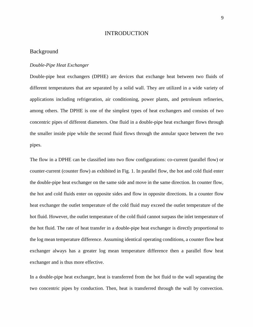
Double-pipe heat exchangers (DPHE) are devices that exchange heat between two fluids of

different temperatures that are separated by a solid wall. They are utilized in a wide variety of

applications including refrigeration, air conditioning, power plants, and petroleum refineries,

among others. The DPHE is one of the simplest types of heat exchangers and consists of two

concentric pipes of different diameters. One fluid in a double-pipe heat exchanger flows through

the smaller inside pipe while the second fluid flows through the annular space between the two

pipes.

The flow in a DPHE can be classified into two flow configurations: co-current (parallel flow) or

counter-current (counter flow) as exhibited in Fig. 1. In parallel flow, the hot and cold fluid enter

the double-pipe heat exchanger on the same side and move in the same direction. In counter flow,

the hot and cold fluids enter on opposite sides and flow in opposite directions. In a counter flow

heat exchanger the outlet temperature of the cold fluid may exceed the outlet temperature of the

hot fluid. However, the outlet temperature of the cold fluid cannot surpass the inlet temperature of

the hot fluid. The rate of heat transfer in a double-pipe heat exchanger is directly proportional to

the log mean temperature difference. Assuming identical operating conditions, a counter flow heat

exchanger always has a greater log mean temperature difference then a parallel flow heat

exchanger and is thus more effective.

In a double-pipe heat exchanger, heat is transferred from the hot fluid to the wall separating the

two concentric pipes by conduction. Then, heat is transferred through the wall by convection.

10

Finally, heat is transferred from the wall to the second fluid in the annular space by convection. It

is desirable to use an inner pipe of a small diameter and made of a material with a high conductivity

to minimize the conduction resistance between the two fluids. In addition, it is often assumed that

the outer surface of the heat exchanger is perfectly insulated, or adiabatic (i.e. no heat is lost to the

surroundings). Finally, heat exchangers can be assumed to be steady-flow devices as they typically

operate for long durations of time without changes in their operating conditions.

Figure 1 Parallel Flow (left) and Counter Flow (right). [1]

Due to the simplicity and wide usage of double-pipe heat exchangers in industrial applications, it

is highly desirable to improve their effectiveness. This is often done through various heat transfer

enhancement techniques. For example, artificially roughening the surface of the pipes (or utilizing

fins) can drastically increase the heat transfer rate when the flow is turbulent. Unfortunately, an

increase in surface roughness results in an increase in pressure drop and thus pumping power.

Bergles denoted that the study of heat transfer improvement is usually represented as heat transfer

enhancement, intensification, or augmentation. In general, that means an increase in the heat

transfer coefficient [2].

11

Heat transfer enhancement methods fall into three main categories: active methods, passive

methods, and compound methods. Mohamad et al. developed a comprehensive review of DPHE

that discussed, in detail, the aforementioned methods used for heat transfer enhancement [3]. The

authors explained that active methods involve the use of an external force to increase heat transfer.

Some examples include: reciprocating plungers, implementing a magnetic field for flow

disturbance, using surface or flow vibration, and applying electromagnetic fields. In passive

methods, no external forces are used for heat transfer enhancement. Instead, surface or geometric

alterations are utilized to enhance the rate of heat transfer. Modifications, such as twisted tape

inserts or fins are very common due to their simplicity, low cost and easy installation and

maintenance. Surface modifications enhance the heat transfer coefficient and thus heat transfer

rate but often result in an increase in pressure drop.

Another passive method of interest involves changes to the geometry of the pipe. This typically

involves altering the cross-section of the heat exchanger. Maximizing the surface area of the wall

between the two fluids improves the efficiency of the heat exchanger but as with surface

treatments, often results in an increase in pressure drop. The compound method of heat transfer

enhancement involves the combination of both passive and active methods, which makes it the

least common of the three.

In this study, a passive method of heat transfer enhancement was investigated, by modifying the

geometry of the inner pipe to increase the surface area of heat transfer. A traditional double-pipe

heat exchanger consists of two concentric pipes with circular cross-sections. In this work, the inner

pipe will be replaced with a pipe with a cross-section inspired by the Koch snowflake fractal

pattern. The use of the Koch snowflake fractal pattern will result in an increase in surface area per

unit volume of the heat exchanger.

12

Koch Snowflake Fractal

Fractals, are never ending patterns that can be found in nature. They are infinitely complex patterns

that repeat a simple process for a finite number of iterations or ad infinitum. Fractal patterns may

be familiar to most because they can be found in nature. Some examples are the vascular system

in plants and animals, human lungs, trees, rivers, coastlines, mountains, clouds, seashells,

snowflakes, among many other. Although they may be only perceived as an infinitely repeating

pattern, fractals have been studied by mathematicians as early as the 17th century for their unique

characteristics. In the present, fractals have played an important role in research among scientists

and engineers. Huang et al. presented some applications of the current use of fractals in heat

transfer. [4].

A fractal pattern of interest is one that was first introduced by Swedish mathematician, Helge von

Koch in 1904. The Koch snowflake is of interest because of its particular behavior. As the number

of fractal iterations increases, so does the perimeter of the Koch snowflake, ad infinitum. However,

while the perimeter could theoretically increase infinitely, the geometry is contained within a finite

area which is dependent on the original size of the zeroth iteration. The Koch Snowflake is built

by starting with an equilateral triangle (zeroth fractal iteration), removing the inner third of each

side, building another equilateral triangle at the location where the side was removed, and then

repeating the process indefinitely. Each repetition is denoted as a fractal iteration. For example,

iteration zero is represented as n = 0, iteration one as n = 1, and so on. The zeroth and first three

fractal iterations of the Koch Snowflake fractal are illustrated in Fig. 2. The number of sides for

the zeroth iteration is that of an equilateral triangle. As the iteration increments Eq. (1) is used to

determine the number of sides.

13

𝑁 = 3 ∗ 4𝑛 (1)

Figure 2 Koch Snowflake Fractal Iterations

The length of the side of the Koch Snowflake, denoted as l, can be calculated by using Eq. (2).

𝑙 = 𝑠 ∗ 3−𝑛 (2)

The perimeter of the Koch Snowflake is dependent on the level of fractal iteration, n, and the

length of the side, s, of the initial equilateral triangle from iteration n = 0. The equation to calculate

the perimeter is presented below in Eq. (3).

𝑃 = (3𝑠) (4

3)

𝑛

(3)

The area of the Koch Snowflake is only dependent on the length of the side, s, of the initial

equilateral triangle of iteration n = 0, as seen in Eq. (4).

𝐴𝑛=0 =√3

4𝑠2 (4)

For iteration n = 1 the area will be the area of the original equilateral triangle plus the area of three

smaller equilateral triangles, as seen in in Eq. (5).

𝐴𝑛=1 =√3

4𝑠2 + 3

√3

4(

𝑠

3)

2

(5)

14

And so on, for iteration n = 2, as seen in Eq. (6) and for iteration n = 3, as seen in Eq. (7).

𝐴𝑛=2 =√3

4𝑠2 + 3

√3

4(

𝑠

3)

2

+ 3 ∗ 4√3

4(

𝑠

32)

2

(6)

𝐴𝑛=3 =√3

4𝑠2 + 3

√3

4(

𝑠

3)

2

+ 3 ∗ 4√3

4(

𝑠

32)

2

+ 3 ∗ 4 ∗ 4√3

4(

𝑠

33)

2

(7)

Generating a summation of a geometric series, whenever n approaches infinity the equation for the

area of the Koch Snowflake simplifies to Eq. (8).

𝐴𝑛→∞ =2√3

5𝑠2 (8)

An increment in perimeter is observed as the Koch Snowflake fractal iteration is increased. For

example, for an initial side length of s = 18 mm, a relationship between perimeter side length ratio

and fractal iteration is observed in Fig. 3. It is observed that for every iteration there is a significant

increase in the perimeter of the geometry. At the fourth fractal iteration, an increase of

approximately 200% of the initial perimeter is experienced.

Figure 3 Perimeter Side Length Ratio and Fractal Iteration

2

4

6

8

10

0 1 2 3 4

P/s

n

15

The relationship of area of the Koch Snowflake and the increment in fractal iteration with same

initial side length of s = 18 mm is illustrated in Fig. 4. The ratio of areas is the area of each iteration

of Koch Snowflake over the area of Koch Snowflake when n approaches infinity. Unlike the

significant increase of perimeter, the area, when compared for each iteration it is observed to be

fundamentally nearly the same. This represents the behavior of the Koch Snowflake fractal. As the

number of fractal iteration increases, the area of the geometry remains finite.

Figure 4 Area Ratio and Fractal Iteration

The Koch Snowflake fractal is special in its behavior. It allows an infinite increase in perimeter

while preserving a finite area. If this concept is translated into a Koch Snowflake pipe geometry

inside a DPHE, conceptually, an infinite surface area can be achieved while maintaining a finite

cross sectional area. A numerical study using computational fluid dynamics of a modified pipe

geometry is presented in this study, and compared to a traditional cylindrical pipe geometry.

0.4

0.6

0.8

1

1.2

0 1 2 3 4

A/A

n→∞

n

16

Motivation

Heat exchangers are widely utilized in industry in a wide range of applications, from heating and

air-conditioning to power production. The simplest type of heat exchanger, the double-pipe heat

exchanger, has garnered very few effective heat transfer enhancements. Improving the

effectiveness of such a commonly utilized heat exchanger is extremely desirable. As passive heat

transfer enhanced methods require no moving mechanical components, they are extremely

desirable. Unfortunately, experimentally examining various passive heat transfer enhancement

methods is both time consuming and expensive due to manufacturing constraints. Fortunately, the

advent of Computational Fluid Dynamics (CFD) has alleviated some of the need for experimental

testing. In this study, the cross-sectional geometry of the inside pipe in a double-pipe heat

exchanger will be modified in accordance with the Koch snowflake pattern. By modifying the

cross-sectional geometry, a significant increase in the surface area available for convective heat

transfer can be achieved without increasing the package volume of the heat exchanger.

Objectives

The objectives of this study is to: (1) create a computational model of a traditional double-pipe

heat exchanger, (2) validate the physics of the model and verify a grid independent solution, (3)

modify the inside pipe to incorporate a fractal cross-section in accordance with the Koch snowflake

pattern, and (4) compare the performance of the fractal heat exchanger to that of a traditional heat

exchanger with a circular cross-section.

Literature Review

In this section, the literature that has been conducted throughout the years to study the performance

of DPHE using computational numerical simulations, is summarized. Numerical simulations have

17

been extensively used to analyze the performance of DPHE to calculate thermal and hydrodynamic

characteristics. Computational fluid dynamics (CFD) is a tool that uses numerical analysis to solve

problems that involve fluid flows. It has been widely used in the study of fluid flow and heat

transfer, including heat exchangers. Several studies have carried experimental and CFD analysis

on heat exchangers to validate the method.

Ibrahim examined important parameters that included heat transfer coefficient and friction factor,

to be able to determine heat transfer rate and pressure drop. He compared the existing theoretical

correlations found in literature, with the CFD, and experimental results. A two-dimensional, and a

k-ε turbulent model were utilized in the numerical simulation setup to find the heat transfer

coefficient. He concluded that the results obtained by CFD were in good agreement with both

experimental data and empirical correlations. Revealing that CFD is an accurate tool to predict

heat transfer coefficient in heat exchanger with turbulent flows [5].

Van der Vyer et al. provided a two-part investigation. First, a three-dimensional simulation of a

DPHE compared CFD, empirical correlations, and experimental results. The simulation was

performed using k-ε for a standard turbulent model. With the assumption of an adiabatic outer

wall, which was not modelled, to help in the reduction of CPU time. The temperature and pressure

at the inlets and outlets were determined so that heat transfer, Nusselt number, and friction factor

could be calculated. When comparing between CFD results and experimental results the average

error was found to be 5.5% with the correlation. It was concluded that the CFD results showed

good agreement. Due to this, it is feasible to model a prototype configuration of a DPHE. The

second part of her investigation, involved using CFD on a modified DPHE design. Although

discussed later into more depth, her investigation, using CFD as a tool, helped in finding the

18

thermal and hydrodynamic characteristics before investing in manufacturing costs and time when

developing a new heat exchanger design [6].

In a numerical investigation, Arslan studied a steady state turbulent forced flow on a DPHE with

a horizontal smooth, semi-circle as the inner pipe. The investigation aimed to compare the Nusselt

number and Darcy friction factor with a modified pipe geometry, but also compare the different

available turbulence models (k-ε Standard, k-ε Realizable, k-ε RNG, k-ω Standard and k-ω SST)

and their results. The results show that as the Reynolds number increased Nusselt number

increased but Darcy friction factor decreased. As for the turbulent models, it was obtained that, k-

ε Standard, k-ε Realizable, and k-ε RNG were the most suitable turbulence models for his

investigation [7].

Kumar et al. presented a work that investigated the hydrodynamic and heat transfer characteristics

of a DPHE. A numerical study of a counter-current configuration with hot fluid in the inner pipe

side and cold fluid in the annulus area, was compared against experimental data. The overall heat

transfer coefficients, Nusselt numbers, and friction factors from the inner and outer pipes were

compared with experimental data collected, as well as reported in the literature. The CFD

simulation results were found to be in good agreement with the experimental data, with Nusselt

number values with 4% error for inner pipe and 10% error in the outer pipe. A reasonable

comparison was found between the literature data and simulations [8].

Bhanuchandrarao et al. conducted a numerical analysis to compare the performance of a parallel

and counter flow DPHE. Using the standard based k-ε turbulence model the analyses were

conducted for three different velocities and seven different fluids. The results of the thermal

performance obtained from the simulations were compared with theoretical correlations. It was

19

concluded that the CFD results were found to be consistent with theoretical calculations with most

valued within 5% of each other [9].

Studies, which have modified the pipe geometry, to maximize surface area, and therefore increase

heat transfer rate, are discussed in detail in the following paragraphs. Chen and Dung studied the

temperature, pressure, and velocity contours. They calculated the Nusselt number and overall heat

transfer coefficient on parallel-flow and counter-flow DPHE with inner pipes of alternating,

horizontal and vertical, oval cross-section pipes. The computational model was simulated using

only laminar flow with a maximum Reynolds number of 2000, and compared to a DPHE with

circular pipes. The results showed that the modification of the pipe’s cross-section geometry

improved the heat transfer performance, in this case with a parallel flow arrangement [10].

Bhadouriya et al. performed three-dimensional numerical simulations for laminar and turbulent

flow regimes to analyze enhancement in heat transfer and pressure drop of air flow inside a twisted

square duct. In their paper the validation of the experimental setup consisted on simulations over

a straight square duct geometry. When comparing the straight square duct against a twisted square

duct geometry, while considering constant pumping criteria, it was concluded that twisted square

duct is more advantageous in laminar flow conditions with an enhancing factor of 10.5 [11].

Meyer and Van der Vyver work is of importance due to the implementation of a fractal pattern on

a DPHE. A quadratic Koch island fractal pipe design was investigated using three techniques: by

analytical, numerical, and experimental methods. The pipe inspired from fractals increases the

pipe’s surface area thus increasing the heat transfer area significantly. As the fractal iterations

increased, heat transfer rate increased. The model targeted the comparison of heat transfer and

pumping power amongst different iterations of fractal pipe geometries. The k-ε model for standard

turbulent flow was used for the simulations. A range of Reynolds numbers of 4500 to 90000 were

20

studied for the pipe, and 3500 to 50000 for the shell. The analytical model was found to be in good

agreement with the numerical predictions in a way that heat transfer increased by a factor of two

for each iteration. The experimental results also confirmed that the numerical simulation results

closely matched the heat transfer increase found [12].

Wang et al. presented a numerical study of turbulent flow and heat transfer of air in a set of regular

polygonal (non-circular) ducts and circular pipe. The k-ε turbulence model was used for ducts with

the same hydraulic diameter as their characteristics lengths in the Reynolds number. The polygonal

geometries simulated included: equilateral triangle, square, regular hexagonal, regular octagonal,

and regular dodecagonal. It was concluded that for a cylindrical pipe, the numerical results agree

well with the experimental correlations. And for the polygonal ducts, the heat transfer coefficient

in the duct corner region is lower than any other part of the wall pipe. The smaller the angle of the

corner region, the more it deteriorated the circumferential local heat transfer coefficient becomes

[13].

Another technique to enhance the thermal performance of a DPHE is the addition of fins to the

pipe to increase surface area, or the addition of inserts to alter the flow behavior. Kumar et al.

investigated the performance of three different DPHE with rectangular, triangular, and parabolic

fin profiles. Numerical analysis was conducted at a various mass flow conditions. A parallel flow

configuration and Reynolds numbers between 100 and 1000. The results suggested a heat transfer

enhancement in the finned pipe compared against the un-finned one [14].

Hameed and Essa provided research of an experimental and numerical investigation to evaluate

the performance of a triangular finned DPHE. The experimental section was conducted on a

smooth and finned pipe heat exchanger. The experimental results showed an enhancement in heat

dissipation for triangular pipes of 3 to 4 times more than the traditional smooth pipe. When

21

comparing with the numerical results, which showed good agreement with a 4% difference

between experimental and numerical results, it was concluded an augmentation in heat transfer in

the triangular finned pipe due to the increase in surface area [15].

Verma and Kumar performed an analysis on a double pipe heat exchanger with helical tap inserts

at the annulus of the inner pipe. With the idea to enhance the thermal characteristics of the heat

exchanger. The Nusselt number and friction factor were obtained from a three-dimensional

simulation using the SST k-ω turbulent model. The results found, were that helical tape inserts in

the annulus increase velocity and surface area enabling the enhancement of heat transfer but also

an increase of pressure drop is observed [16].

In an innovative design, Hashenheim et al. studied a DPHE with conical pipes. The modified

geometry improved thermal performance while reducing the weight of the device. The simulations

were performed for Reynolds number from 12000 to 50000 using the k-ε turbulence model.

Parameters, such as the Nusselt number and friction factor were numerically investigated. It was

concluded that the modified conical geometry of the DPHE produced an increase in heat transfer

rate of 54% and Nusselt number incremented by 63% [17].

A summary of the aforementioned literature indicates that an increase in heat transfer can achieved

through modifications to the surface of the heat exchanger. What has received little attention is the

use of fractal geometries in the design of heat exchangers. In this study, the Koch snowflake pattern

will be utilized to increase the convective surface area of a double-pipe heat exchanger without

changing the package volume. The performance of this fractal heat exchanger will be compared

with that of a traditional double-pipe heat exchanger.

22

CHAPTER 1: HEAT TRANSFER IN A FRACTAL DPHE

Introduction

Passive methods for heat transfer enhancement techniques are common in a DPHE. When

analyzing the performance of double-pipe heat exchangers it is important to note the difference

between thermal performance and hydraulic performance. If the goal is to minimize pressure drop,

and thus pumping power, modifications to the surface are sometimes undesirable. However, if the

goal is to increase the surface area to volume ratio of the heat exchanger than surface modifications

are often advantageous. This work will focus on heat transfer enhancement rather than pumping

power minimization. In this study, heat transfer enhancement will be achieved by modifying the

cross-sectional geometry of the inside pipe in a double-pipe heat exchanger in accordance with the

Koch snowflake fractal pattern. The increase in surface area that can be achieved with the Koch

snowflake design is highly dependent upon the fractal iteration. Therefore, double-pipe heat

exchangers with cross-sections in accordance with the first three fractal iterations of the Koch

snowflake fractal pattern will be investigated.

Heat Transfer Analysis on Koch Snowflake DPHE

Heat transfer inside a DPHE consists of exchange of thermal energy between a cold fluid and a

hot fluid with a solid wall (pipe) separating both. Three heat transfer operations occur: convective

heat transfer from the inner fluid to the inner wall of the pipe, conductive heat transfer through the

pipe wall, and convective heat transfer from the outer pipe wall to the outside fluid. In this section,

some theoretical correlations for the heat transfer analysis of a DPHE are introduced. The heat

transfer rate, overall heat transfer coefficient, and effectiveness are explained in this section for

23

further understanding of the heat transfer enhancement of the Koch Snowflake DPHE. To find the

rate of heat transfer between the two fluids the following equation Eq. (9) is applied

�� =Δ𝑇

𝑅= 𝑈𝐴𝑠Δ𝑇𝑙𝑚 (9)

where R is the total thermal resistance that associates both convection and conduction as seen in

Eq. (10), ΔT is the log mean temperature difference, As the surface area of the wall, and U is the

overall heat transfer coefficient expressed in Eq. (11),

𝑅 =1

ℎ𝑖𝐴𝑖+

log𝐷𝑜

𝐷𝑖

2𝜋𝑘𝐿+

1

ℎ𝑜𝐴𝑜 (10)

𝑈 =1

𝑅𝐴𝑠 (11)

where hi and ho are the heat transfer coefficients of the fluids and k is the thermal conductivity of

the wall, Di and Do, inner and outer hydraulic diameters, respectively. And, Ai and Ao the inner

surface of the wall and outer surface of the wall separating the two fluids, respectively. The heat

transfer coefficient for either cold or hot fluids is expressed as in Eq. (12),

ℎ = 𝑘𝑁𝑢

𝐷ℎ (12)

where k is the thermal conductivity of the cold or hot fluid, Dh the hydraulic diameter and Nu the

Nusselt number found by using the Gnielinski correlation for turbulent flows as in Eq. (13),

𝑁𝑢 =(

𝑓8) (𝑅𝑒 − 1000)𝑃𝑟

1 + 12.7 (𝑓8)

12

(𝑃𝑟23 − 1)

(13)

where Pr is the Prandtl number, Re the Reynolds number, and f is the friction factor later described

in Chapter 2.

24

In order to increase the rate of heat transfer in a double-pipe heat exchanger the overall heat transfer

coefficient must be increased. Alternatively, the surface area of the heat exchanger could be

increased. It should be noted that the surface area of the heat exchanger should be increased

without increasing the package volume of the heat exchanger. This can be accomplished with the

Koch snowflake fractal pattern. By increasing the surface area of the heat exchanger through the

use of the Koch snowflake fractal pattern, an increase in the total heat transfer rate should be

achieved.

It should be noted that the log mean temperature difference method used in the analysis of heat

exchangers is used to determine the size of a heat exchanger to achieve prescribed outlet

temperatures when the operating conditions are known. In this analysis, the size of the heat

exchanger is known because the size of the pipes are already defined by the Koch snowflake fractal

pattern. Thus, the log mean temperature difference method is not suitable for this analysis. In this

analysis, the rate of heat transfer and fluid outlet temperatures should be determined in order to

characterize the performance. Again, in this case, the operating conditions (flow rates and inlet

temperatures) and size of the heat exchanger are known. The goal of this study is to determine the

heat transfer performance of double-pipe heat exchangers inspired by the Koch snowflake fractal

pattern. Therefore, the effectiveness-NTU method will be employed rather than the log mean

temperature difference method. The effectiveness of the heat exchanger is the ratio of the actual

heat transfer rate to the maximum possible heat transfer rate. NTU stands for the Number of

Transfer Units and it is largely a measure of the size, or heat transfer area, of the heat exchanger.

If the effectiveness, ε, is obtained through equation Eq. (14), specifically for counter flow

configurations, then it is possible to calculate the rate of heat transfer.

25

휀 =1 − e(−NTU(1−c))

1 − (𝑐𝑒(−𝑁𝑇𝑈(1−𝑐))) (14)

where c, is the heat capacity ratio as seen in equation Eq. (15) and NTU is the number of transfer

units obtained by equation Eq. (16) as follows

𝑐 =𝐶𝑚𝑖𝑛

𝐶𝑚𝑎𝑥 (15)

𝑁𝑇𝑈 =𝑈𝐴𝑠

𝐶𝑚𝑖𝑛 (16)

where Cmin is the smaller heat capacity rate which will experience a larger temperature change.

Using this concept, it is possible to obtain the maximum heat transfer rate as in Eq. (17), and

consequently the actual rate of heat transfer using equation Eq. (18).

��𝑚𝑎𝑥 = 𝐶𝑚𝑖𝑛(𝑇ℎ,𝑖𝑛 − 𝑇𝑐,𝑖𝑛) (17)

�� = 휀��𝑚𝑎𝑥 (18)

26

CHAPTER 2: COMPUTATIONAL FLUID DYNAMICS

Introduction

In this section, a computational fluid dynamics model of a traditional double-pipe heat exchanger

and several fractal double-pipe heat exchangers will be developed. The computational model’s

physics will be validated with known theoretical solutions. In addition, the computational models

will be verified for grid independent solutions. After validating and verifying the computational

models, the performance of a double-pipe heat exchanger with a fractal cross-section will be

compared with that of a traditional double-pipe heat exchanger with a circular cross-section.

Koch Snowflake DPHE

A three-dimensional DPHE with a modified Koch Snowflake fractal inner pipe was modeled using

SolidWorks, a commercially available CAD software. Four different models were generated, one

for each of the first three fractal iterations, and one for a traditional circular cross section pipe

geometry for comparison and validation purposes. The dimensions of the traditional DPHE are

shown in Table 1.

Table 1 Dimensions of Double Pipe Heat Exchanger

DPHE Dimensions (mm)

Inner Pipe Diameter 15

Inner Pipe Thickness 2

Outer Pipe Diameter 32

Pipe Length 1000

A zoom-in of the solid geometry of the inner fluid, inner cylindrical pipe, and outer fluid of the

DPHE with the dimensions of Table 1 is shown in Fig. 5. The origin and axis of reference for XY

27

and YZ are illustrated in Fig. 6. These reference axes are of relevance to understand the orientation

of the thermal contours obtained and exhibited further into the study. The outer pipe of the DPHE

was not modeled, but it was still taken into consideration. In other words, it was assumed that the

outer surface of the heat exchanger was perfectly insulated, or adiabatic.

Figure 5 Close-Up View of DPHE Solid Model

Figure 6 Origin and Axis of Reference of DPHE in Millimeters

0

0

1000

-16

16

7.5

-7.5

Outer Cold Fluid

Inner Copper Pipe

Inner Hot Fluid

28

The modified Koch Snowflake pipes for iteration n = 0, n = 1, and n = 2 were also modeled using

SolidWorks. The pipe thickness was representative of a traditional pipe thickness, based on the

wall schedule, for the pipe hydraulic diameter used in this analysis. The three different pipes are

illustrated in Fig. 7. Notice how iteration n = 0 is a simple equilateral triangle and iteration n = 2

begins to take shape of a snowflake. The increase of the surface area for every increment in

iteration is clearly noticeable, especially when comparing between iteration n = 0 and iteration n

= 2. The initial length of one of the sides of the equilateral triangle from iteration n = 0 is 18 mm.

The side lengths of the other smaller triangles in the following iterations can be found by using

Eq. (2) previously introduced.

Figure 7 Modified Koch Snowflake Pipes

Computational Methodology

Governing Equations

The numerical simulations used to analyze the modified heat exchanger’s thermal performance

were performed in ANSYS Fluent 17.1. The Reynolds Averaged Navier-Stokes (RANS) were

utilized in this analysis as turbulent flow was considered. The equations governing the fluid flow

n = 0 n = 1 n = 2

29

and heat transfer are discussed into more detail below. The continuity and momentum equation are

shown in Eq. (19) and Eq. (20), respectively.

∂ρ

∂t+ ∇ ∙ (ρ��) = 𝑆𝑚 (19)

∂ρ

∂t(ρ��) + ∇ ∙ (𝜌��) = −∇p + ∇ ∙ (𝜏) + 𝜌�� + �� (20)

In the continuity equation, ρ is the density of the fluid, v the velocity, and Sm is the mass added to

the continuous phase. In the momentum equation, p is the static pressure, 𝜏 is the stress tensor

displayed in Eq. (21), and ρ�� and �� are the gravitational body forces and external body forces,

respectively. The stress tensor previously mentioned is given by

𝜏 = μ[(∇�� + ∇��𝑇)] −2

3∇ ∙ ��𝐼 (21)

where μ is the molecular viscosity, I the unit tensor, and the second term on the right-hand side is

the effect of volume dilation.

Turbulence Model

As the flow in most industrial heat exchangers applications is turbulent, a turbulence model was

utilized in the computational simulations. Specifically, the realizable k-ε turbulent model proposed

by Shih et al. was selected for this study [18]. The k-ε turbulence model has been extensively

validated for a wide range of flows [19]. The modeled transport equations for k and ε in the

realizable k-ε model can be seen in Eq. (22) and Eq. (23), respectively.

∂

𝜕𝑡(𝑝𝑘) +

∂

𝜕𝑥𝑗(𝑝𝑘𝑢𝑗) =

∂

𝜕𝑥𝑗[(μ +

μ

𝜎𝜀)

𝜕휀

𝜕𝑥𝑗] + 𝐺𝑘 + 𝐺𝑏 − 𝜌휀 − 𝑌𝑀 + 𝑆𝑘 (22)

and

30

∂

𝜕𝑡(𝑝휀) +

∂

𝜕𝑥𝑗

(𝑝휀𝑢𝑗) =∂

𝜕𝑥𝑗[(μ +

μ

𝜎𝜀)

𝜕휀

𝜕𝑥𝑗] + 𝜌𝐶1𝑆휀 − 𝜌𝐶2

휀2

𝑘 + √𝜐휀+ 𝐶1𝜀

휀

𝑘𝐶3𝜀𝐺𝑏 + 𝑆𝜀 (23)

where

𝐶1 = 𝑚𝑎𝑥 [0.43,𝜂

𝜂 + 5] , 𝜂 = 𝑆

𝑘

휀 𝑆 = √2𝑆𝑖𝑗𝑆𝑖𝑗 (24)

In these equation, Gk represents the generation of turbulence kinetic energy due to mean velocity

gradients, Gb is the generation of turbulent kinetic energy due to buoyancy, YM is the contribution

of the fluctuating dilatation in compressible turbulence to the overall dissipation rate. C2 and C1ε

are constants. Then, σk and σε are the turbulent Prandtl numbers for k and ε, respectively. Sk and Sε

are user defined source terms. The model for turbulent eddy viscosity is presented in the following

Eq. (25).

𝜇𝑡 = 𝜌𝐶𝜇

𝑘2

휀 (25)

The Cμ in the realizable k-ε models is not constant and calculated as seen in Eq. (26)

𝐶𝜇 =1

𝐴0 + 𝐴𝑠𝑘𝑈∗

휀

(26)

where,

𝑈∗ = √𝑆𝑖𝑗𝑆𝑖𝑗 + Ω𝑖𝑗Ω𝑖𝑗 (27)

and,

Ω𝑖𝑗 = Ω𝑖𝑗 − 2휀𝑖𝑗𝑘𝜔𝑘 (28)

Ω𝑖𝑗 = Ω𝑖𝑗 − 2휀𝑖𝑗𝑘𝜔𝑘 (29)

where Ω𝑖𝑗 is the mean rate-of-rotation tensor viewed on a moving reference frame with an angular

velocity ωk. The model constants A0 and As are given by

31

A0 = 4.04, A𝑠 = √6 cos 𝜙

where finally,

𝜙 =1

3cos−1(√6𝑊), 𝑊 = 𝑆𝑖𝑗𝑆𝑖𝑘𝑆𝑘𝑖 , �� = √𝑆𝑖𝑗𝑆𝑖𝑗, 𝑆𝑖𝑗 =

1

2(

𝜕𝑢𝑗

𝜕𝑥𝑖+

𝜕𝑢𝑖

𝜕𝑥𝑗) (30)

and the constant variables of the model are:

𝐶1𝜀 = 1.44, C2 = 1.9, σ𝑘 = 1.0, σ𝜖 = 1.2

Heat Transfer Model

ANSYS Fluent is also capable of solving heat transfer through the energy equation. Heat transfer

within the fluid and/or a solid can be solved simultaneously. A model of a DPHE is a perfect

example of the capabilities of this software. Where convection is occurring within a fluid, and

conduction through the solid pipes. To include heat transfer in the model, certain parameters must

be taken into consideration. Such as thermal boundary conditions and material properties that

govern heat transfer, which may vary with temperature. The energy equation being solved for a

turbulent model is shown in Eq. (31).

𝜕

𝜕𝑡(𝜌𝐸) +

𝜕

𝜕𝑥𝑖

[𝑢𝑖(𝜌𝐸 + 𝑝)] =𝜕

𝜕𝑥𝑗(𝑘𝑒𝑓𝑓

𝜕𝑇

𝜕𝑥𝑗+ 𝑢𝑖(𝜏𝑖𝑗)

𝑒𝑓𝑓) + 𝑆ℎ (31)

where (τij)eff is the deviatoric stress sensor, defined in Eq. (32). E is the total energy as seen in Eq.

(33), and keff is the effective thermal conductivity shown in Eq. (35),

(𝜏𝑖𝑗)𝑒𝑓𝑓

= 𝜇𝑒𝑓𝑓 (𝜕𝑢𝑗

𝜕𝑥𝑖+

𝜕𝑢𝑖

𝜕𝑥𝑗) −

2

3𝜇𝑒𝑓𝑓

𝜕𝑢𝑘

𝜕𝑥𝑘𝛿𝑖𝑗 (32)

𝐸 = ℎ −𝑝

𝜌+

𝑣2

2 (33)

where h for an incompressible flow is defined as seen in Eq. (34),

32

ℎ = ∑ 𝑌𝑗ℎ𝑗 +𝑝

𝜌𝑗

(34)

and for realizable k-ε models, the effective thermal conductivity is given by

𝑘𝑒𝑓𝑓 = 𝑘 +𝑐𝑝𝜇𝑡

𝑃𝑟𝑡 (35)

where k is the thermal conductivity, and the default value of the turbulent Prandtl number is 0.85.

The previously described governing equations for continuity, momentum, and energy are the

general version that can be applicable to any turbulent model. Depending on the application, some

of the terms are not taken into consideration. By establishing assumptions to the model, it is

possible to simplify these equations. In this study the assumptions taken were:

1. Heat exchangers usually operate for long periods of time with no change in their operating

conditions. Therefore, they can be modeled as steady-state flow devices.

2. The fluid streams experience little to know change in their velocities and elevations, and

thus the kinetic and potential energy changes are negligible.

3. The fluid (water) being used is incompressible and thus the density can be assumed to be

constant.

4. Axial heat conduction along the pipe is usually insignificant, and can be considered

negligible in most theoretical analysis. However, it is taken into account in the

computational model.

5. The outer surface of the heat exchanger is assumed to be perfectly insulated, so there is no

heat loss to the surrounding medium, and heat transfer occurs between the two fluids only.

In this manner, the rate of heat transfer of the hot fluid is equal to that of the cold fluid.

6. The working fluid, single phase water, was assumed to have temperature-dependent

thermophysical and rheological properties.

33

With these assumptions taken into consideration, the simplified continuity Eq. (36), momentum

Eq. (37), and energy Eq. (38) equations are displayed as follows. Assuming a steady-state, and

temperature dependent thermophysical and rheological properties, the continuity equation, in its

reduced form is

∇(𝜌��) = 0 (36)

Similarly, assuming a steady-state, temperature dependent properties, and negligible gravitational

body forces, the momentum equation can be reduced to

∇(𝜌��) = −∇p + ∇(𝜏) (37)

where the stress tensor is given by

𝜏 = 𝜇∇�� (38)

Once again assuming a steady-state, temperature dependent properties, and the energy equation

can be simplified to

∇(��(𝜌𝐸 + 𝑝)) = ∇ (𝑘∇𝑇 + (𝜏��𝑓𝑓��)) (39)

where the total energy is given by

𝐸 = ℎ −𝑝

𝜌+

𝑣2

2 (40)

Neglecting the flow work and kinetic energy terms, the energy equation simplifies to

∇(��(𝜌ℎ)) = ∇ (𝑘∇𝑇 + (𝜏��𝑓𝑓��)) (41)

where the enthalpy is defined as

ℎ = 𝑐𝑝𝑇 (42)

34

Mesh Generation

The DPHE being studied, was discretized to employ the finite volume method. The governing

equations for mass, momentum and energy are solved on these set of control volumes. The quality

of the mesh in a numerical simulation is of critical importance. The mesh structure and refinement

play an important role in obtaining a high degree of accuracy, and obtaining the solution in a

reasonable amount of computational time. A balance between the two will provide an optimum

mesh.

A series of steps were taken to create the mesh of four different models: the traditional DPHE with

circular pipe, and iterations n = 0, n = 1, and n = 2 of the modified Koch Snowflake DPHE. All

the geometries were imported to ANSYS Design Modeler from SolidWorks. They were simplified,

defeatured, and translated to have a consistent orientation. For the traditional DPHE with circular

pipe, a structured hexahedral mesh with a swept method was implemented as seen in Fig. 8. The

mesh was refined locally using sizing and inflation layers to properly capture the boundary layer,

a cross-sectional view of the mesh is illustrated in Fig. 9. The calculated height of the first layer

thickness, using the appropriate y+ values, was taken into consideration in the mesh generation, as

seen in Fig. 10. The hexahedral mesh with a swept method was set for 250 divisions along the z-

axis as illustrated in Fig. 11. The total number of elements produced was approximately 1.3

million.

35

Figure 8 Mesh Structure for Cylindrical Pipe DPHE

Figure 9 Mesh Structure of Circular Cross-Section

36

Figure 10 Zoomed in View of Inflation Layers to Capture Boundary Layer

Figure 11 Mesh Structure along Z-Axis

Outer Cold Fluid Copper Pipe Inner Hot Fluid

Inflation Layers

Outer Cold Fluid

Outer Cold Fluid

Inner Hot Fluid Copper Pipe

37

The mesh for the zeroth to the second iteration of the Koch Snowflake DPHE were generated in a

similar manner. They consist of mostly hexahedral and wedge elements, which are highly

encouraged for a mesh in computational fluid analysis. The corresponding first layer thickness for

each fractal iteration was also calculated and the proper inflation layer for the fluid domains was

added. The mesh structures of the cross-section of the Koch Snowflake fractal for iteration n = 0

is illustrated in Fig. 12, iteration n = 1 in Fig. 13, and iteration n = 2 in Fig. 14.

Figure 12 Mesh Structure of Koch Snowflake DPHE Cross-Section Iteration n = 0

n = 0

38



n = 2

n = 1

39

The quality of the mesh has a significant impact on the accuracy and stability of the numerical

solution. Checking for mesh quality is essential in numerical solutions. To check for mesh quality

several mesh metrics are available. One of the most common methods of checking the quality of

the mesh is the cell skewness. The skewness is defined as the difference between the shape of the

cell and the shape of the equilateral cell of equivalent volume. Highly skewed cell can decrease

the accuracy of the numerical solution. A general rule of thumb for checking skewness is the

following: if the skewness value is 0-0.25 (excellent), 0.25-0.50 (very good), 0.50-0.80 (good),

0.80-0.94 (acceptable), 0.95-0.97 (bad), and 0.98-1.00 (unacceptable). The skewness and number

of elements for each geometry being studied was recorded and can be seen in Table 2.

Table 2 Skewness and Number of Elements for Each Geometry

Geometry Number of Elements Skewness (Max) Skewness (Average)

Traditional 1,311,000 0.49 0.05

Iteration 0 1,885,750 0.72 0.20

Iteration 1 1,982,000 0.71 0.31

Iteration 2 4,865,500 0.70 0.21

Boundary Conditions

In a numerical simulation, the conditions that are observed in a real-life experiment are adopted.

The initial fluid and thermal boundary conditions are described in this section. The model consists

of two inlets and two outlets. The inlets consider an inlet velocity and the outlets a pressure outlet.

Uniform inlet velocities were utilized. The magnitude of the inlet velocity was changed to achieve

prescribed inlet Reynolds numbers. It should be noted that in order to calculate the Reynolds

number, a hydraulic diameter had to be calculated for each of the fractal heat exchangers due to

their non-circular cross-sectional geometries. Simulations, for a range of Reynolds numbers from

40

10000 to 40000 were performed in increments of 5000. Note that this Reynolds number range

corresponds to a turbulent flow regime. The pressure outlets are the same throughout all models

considering an atmospheric (zero-gauge) pressure outlet at an ambient temperature of 30°C (303

K). The working fluid, in the inner pipe as well as in the annular space, was assumed to be

incompressible and single phase water. The inner pipe was composed of copper with constant

thermophysical properties. It was assumed that there was no velocity slip at all walls. The outer

pipe, composed of aluminum, was assumed to be perfectly insulated. The inlet temperatures were

20°C for the cold fluid and 60°C for the hot fluid. The heat-exchangers were assumed to operate

in the counter-flow configuration. An overview of the boundary conditions imposed to the DPHE

are illustrated in Fig. 15.

Figure 15 Overview of Initial Boundary Conditions

Pressure Outlet (Hot)

Copper Inner Wall

Inlet Velocity (Hot)

Adiabatic Outer Wall

Pressure Outlet (Cold)

Inlet Velocity (Cold)

41

Solution Methods

Pressure-velocity coupling was achieved via the SIMPLE (Semi-Implicit Method for Pressure

Linked Equations) method which uses a relationship between velocity and pressure corrections to

enforce mass conversation and to obtain the pressure field.

The CFD software stores discrete values of field variables at cell centers. However, face values

are required for the convective term and must be interpolated from the cell center values. This was

accomplished via the QUICK (Quadratic Upstream Interpolation for Convective Kinematics)

scheme due to the use of hexahedral elements. A second order scheme was utilized to interpolate

pressure values at cell faces. Gradients required to construct scalar values of field variables at cell

faces as well as for determining secondary diffusion terms and velocity derivatives were calculated

according to the Least Squares Cell-Based method.

The pressure based solver utilizes under-relaxation to control the update of computed variables at

each iteration. Under-relaxation factors for pressure and momentum were 0.3 and 0.7 and for

energy was 0.9.

Validation

The numerical simulation results were compared to theoretical correlations for validation of the

model. The theory provides correlations that are useful for solving fluid and thermal characteristics

of a system. The theoretical equations to solve for pressure drop, friction factor, and Reynolds

number were obtained from Cengel et al. [1]. The pressure drop was analytically calculated for the

traditional DPHE using the theoretical correlations and compared to the numerical simulation

outlet pressures.

42

The pressure drop for the analytical solution is given by Eq. (43).

𝑃𝐿 = 𝑓𝐿

𝐷ℎ

𝜌𝑣2

2 (43)

where f is the friction factor obtained using the the Haaland equation, Eq. (44), which is an

approximation of the Colebrook-White equation that iteratively solves the Darcy-Weisbach

friction factor formula, v is velocity calculated by Eq. (45) and L is the length of the pipe.

1

√𝑓= −1.8 log [(

𝜖𝐷ℎ

3.7)

1.11

+6.9

𝑅𝑒] (44)

𝑣 =𝑅𝑒 𝜈𝑘

𝐷ℎ (45)

In the equation above ε is the pipe roughness, vk the kinematic viscosity, and Dh the hydraulic

diameter calculated by Eq. (46).

𝐷ℎ =4𝐴

𝑃 (46)

The hydraulic diameter was of critical importance in the analytical solution since the cross-section

area, A, and the perimeter, P, of the Koch Snowflakes varied per iteration. This resulted in modified

velocities to achieve a constant Reynolds number. For the validation, only the equations for a

circular cross section were used. The analytical pressure drop for the inlet of the hot fluid was

found to be in good agreement with the numerical solutions as illustrated in Fig.16. A close

agreement can also be observed for the cold fluid inlet pressure as illustrated in Fig. 17.

43

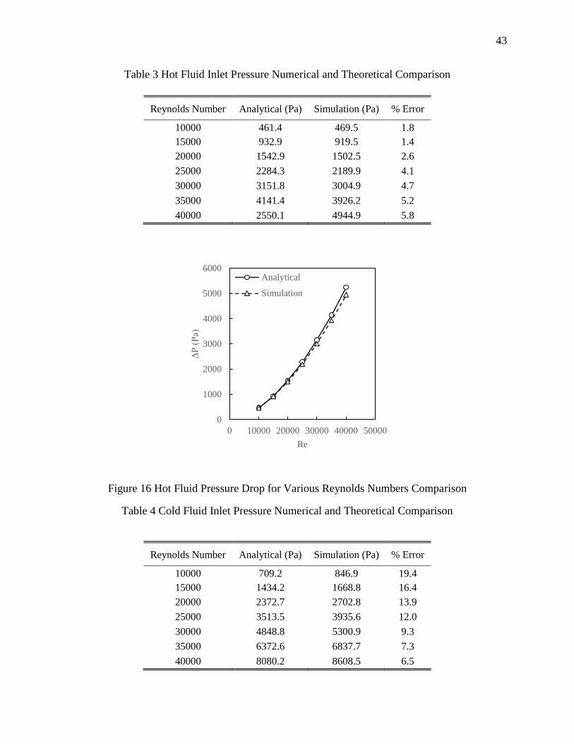
Table 3 Hot Fluid Inlet Pressure Numerical and Theoretical Comparison

Reynolds Number Analytical (Pa) Simulation (Pa) % Error

10000 461.4 469.5 1.8

15000 932.9 919.5 1.4

20000 1542.9 1502.5 2.6

25000 2284.3 2189.9 4.1

30000 3151.8 3004.9 4.7

35000 4141.4 3926.2 5.2

40000 2550.1 4944.9 5.8

Figure 16 Hot Fluid Pressure Drop for Various Reynolds Numbers Comparison

Table 4 Cold Fluid Inlet Pressure Numerical and Theoretical Comparison

Reynolds Number Analytical (Pa) Simulation (Pa) % Error

10000 709.2 846.9 19.4

15000 1434.2 1668.8 16.4

20000 2372.7 2702.8 13.9

25000 3513.5 3935.6 12.0

30000 4848.8 5300.9 9.3

35000 6372.6 6837.7 7.3

40000 8080.2 8608.5 6.5

0

1000

2000

3000

4000

5000

6000

0 10000 20000 30000 40000 50000

ΔP

(P

a)

Re

Analytical

Simulation

44

Figure 17 Cold Fluid Pressure Drop for Various Reynolds Numbers Comparison

Verification

To verify that the mesh was grid-independent, meaning that the mesh structure obtained is the

suitable one for this study, a grid sensitivity analysis was performed. A fine enough mesh is

required for an accurate solution, but at the same time computational time is of essence. The goal

of a grid-independence study is to monitor an important solution variable, in this case the inlet

static pressure, and ensure that the solution variable does not change with further refinement of the

mesh density. The pressure drop as a function of the number of cells can be seen in Fig. 18. It is

seen that after approximately 1.3 million elements the inlet static pressure (gage) is approaching

an asymptotic value. Further increasing the density of the mesh would increase computational time

but would not greatly impact the accuracy of the solution. It should be noted that a tradeoff is

always made between computational time and what is deemed as an acceptable level of accuracy.

The number of cells in a computational domain is directly related to the computational time

required.

0

2000

4000

6000

8000

10000

0 10000 20000 30000 40000 50000

ΔP

(P

a)

Re

Analytical

Simulation

45

Figure 18 Verification of Grid-Independence

Results

Having validated a computational model of a traditional double-pipe heat exchanger with a

theoretical solution and also verifying the solution for grid independence, a computational model

of a fractal double-pipe heat exchanger can be examined. The surface area of a heat exchanger

with a fractal cross-section in accordance with the Koch snowflake fractal pattern is highly-

dependent upon fractal iteration. An approximation of the inner pipe surface area for the traditional

as well as for the first three iterations of the Koch snowflake fractal pattern can be seen in the table

below.

Table 5 Heat Transfer Surface Area of Inner Pipe

Geometry Surface Area (mm2)

Traditional 47000

Iteration 0 54000

Iteration 1 72000

Iteration 2 96000

410

420

430

440

450

460

470

480

0.E+00 5.E+05 1.E+06 2.E+06 2.E+06

ΔP

(P

a)

Number of Elements

46

Overall Heat Transfer Coefficient

The heat transfer coefficients for the hot and cold fluids were obtained from the simulations and

used to evaluate the total thermal resistance using Eq. (10). The conduction resistance in the inner

pipe wall was assumed to be negligible. This was because the inner pipe was composed of copper

of a relatively thin thickness. As the thickness was relatively small, and the thermal conductivity

of copper is relatively high, there is a fairly negligible conduction resistance for the inner pipe

wall. On the other hand the increase in surface area, associated with increases in fractal iteration,

directly impacts the overall heat transfer coefficient. A plot of the overall heat transfer coefficient

as a function of inlet Reynolds number and fractal iteration can be seen in Fig. 19. As expected,

an increase in the inlet Reynolds number resulted in an increase in the overall heat transfer

coefficient. As the number of fractal iterations increased, so did the overall heat transfer

coefficient, largely due to the increase in available surface area for convective heat transfer.

Figure 19 Overall Heat Tranfer Coefficient as a Function of Reynolds number

1000

2000

3000

4000

5000

6000

10000 20000 30000 40000

U (

W/m

2∙K

)

Re

n = 0

n = 1

n = 2

47

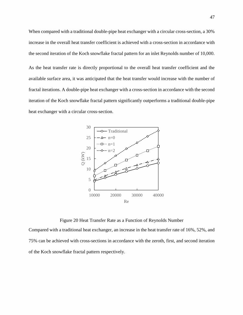
When compared with a traditional double-pipe heat exchanger with a circular cross-section, a 30%

increase in the overall heat transfer coefficient is achieved with a cross-section in accordance with

the second iteration of the Koch snowflake fractal pattern for an inlet Reynolds number of 10,000.

As the heat transfer rate is directly proportional to the overall heat transfer coefficient and the

available surface area, it was anticipated that the heat transfer would increase with the number of

fractal iterations. A double-pipe heat exchanger with a cross-section in accordance with the second

iteration of the Koch snowflake fractal pattern significantly outperforms a traditional double-pipe

heat exchanger with a circular cross-section.

Figure 20 Heat Transfer Rate as a Function of Reynolds Number

Compared with a traditional heat exchanger, an increase in the heat transfer rate of 16%, 52%, and

75% can be achieved with cross-sections in accordance with the zeroth, first, and second iteration

of the Koch snowflake fractal pattern respectively.

0

5

10

15

20

25

30

10000 20000 30000 40000

Q (

kW

)

Re

Traditional

n=0

n=1

n=2

48

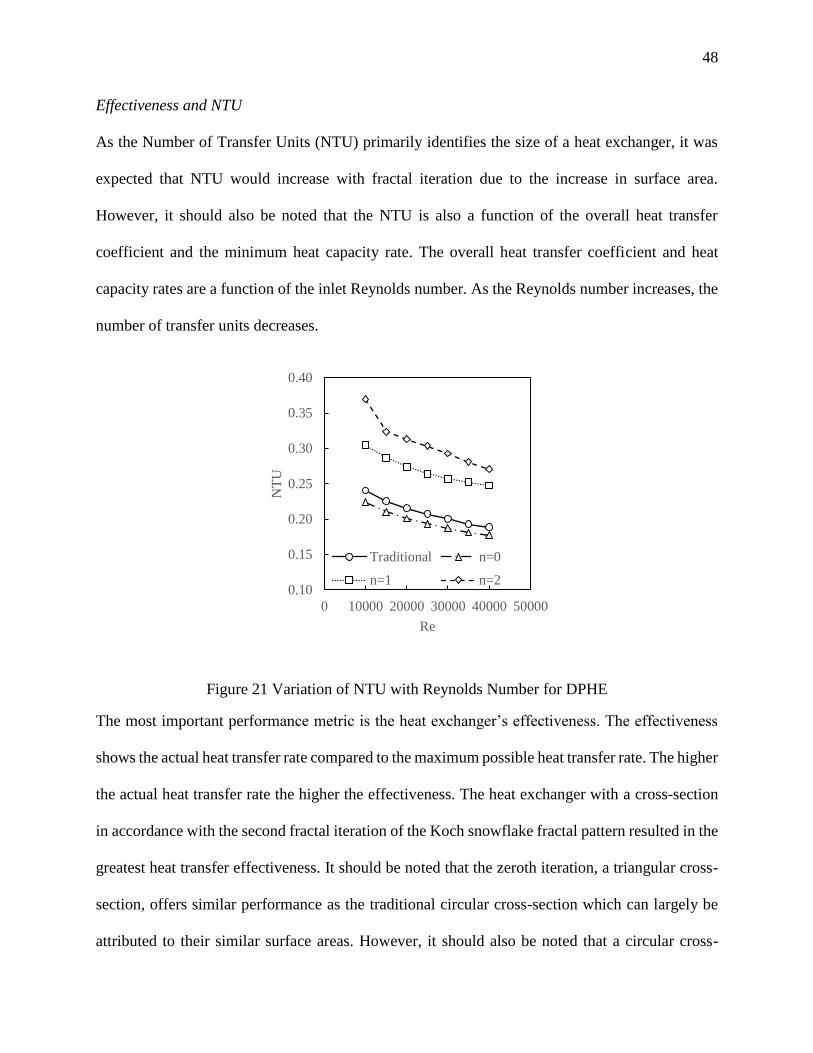
Effectiveness and NTU

As the Number of Transfer Units (NTU) primarily identifies the size of a heat exchanger, it was

expected that NTU would increase with fractal iteration due to the increase in surface area.

However, it should also be noted that the NTU is also a function of the overall heat transfer

coefficient and the minimum heat capacity rate. The overall heat transfer coefficient and heat

capacity rates are a function of the inlet Reynolds number. As the Reynolds number increases, the

number of transfer units decreases.

Figure 21 Variation of NTU with Reynolds Number for DPHE

The most important performance metric is the heat exchanger’s effectiveness. The effectiveness

shows the actual heat transfer rate compared to the maximum possible heat transfer rate. The higher

the actual heat transfer rate the higher the effectiveness. The heat exchanger with a cross-section

in accordance with the second fractal iteration of the Koch snowflake fractal pattern resulted in the

greatest heat transfer effectiveness. It should be noted that the zeroth iteration, a triangular cross-

section, offers similar performance as the traditional circular cross-section which can largely be

attributed to their similar surface areas. However, it should also be noted that a circular cross-

0.10

0.15

0.20

0.25

0.30

0.35

0.40

0 10000 20000 30000 40000 50000

NT

U

Re

Traditional n=0

n=1 n=2

49

section is the most desirable from the perspective of minimizing pumping power. It was not the

goal of this analysis to analyze the hydrodynamic performance but rather the thermal performance

of heat exchangers with fractal geometries.

Contour plots of fluid temperature can be found in the Appendix for both the traditional as well as

the Koch snowflake inspired fractal heat exchangers.

Figure 22 Effectiveness as a Function of NTU

0.10

0.15

0.20

0.25

0.30

0.35

0.40

0.1 0.15 0.2

ε

NTU

Traditional

n=0

n=1

n=2

50

CONCLUSIONS

A thermal performance of a traditional double-pipe heat exchanger with a circular cross-section

was compared to the performance of double-pipe heat exchangers with cross-section in accordance

with the first three fractal iterations of the Koch snowflake pattern. The computational models

were validated with a theoretical model for pressure drop and verified for grid independence

through a mesh sensitivity analysis. The benefit of the use of the Koch snowflake design is that an

increase in surface area can be achieved without impacting package volume. Thus, heat exchangers

with fractal designs have significantly higher surface areas per unit package volume when

compared with traditional heat exchangers. The increase in surface area associated with each

fractal iteration resulted in higher overall heat transfer coefficients and heat transfer rates. In

addition, the effectiveness of the fractal heat exchangers was greater than that of the traditional

heat exchanger, regardless of iteration. As the number of fractal iterations increased, the

effectiveness also increased. It is hypothesized that further iterations may result in an additional

increase in effectiveness. Future studies may need to examine the tradeoff between increase in heat

transfer and increasing in pumping power requirements.

51

REFERENCES

[1] Y. A. Cengel and G. J. Afshin, Heat and Mass Transfer: Fundamentals & Applications, New

York: McGraw-Hill, 2011.

[2] E. A. Bergles, "The Imperative to Enhance Heat Transfer," in Heat Transfer Enhancement

of Heat Exchangers, Springer Netherlands, 1999, pp. 13-29.

[3] M. Omidi, M. Farhadi and M. Jafari, "A Comprehensive Review on Double Pipe Heat

Exchangers," Applied Thermal Engineering, pp. 1075-1090, 2017.

[4] Z. Huang, Y. Hwang, V. Aute and R. Radermacher, "Review of Fractal Heat Exchangers,"

in International Refrigeration and Air Conditioning Conference, West Lafayette, 2016.

[5] G. H. Ibrahim, "Experimental and CFD Analysis of Turbulent Flow Heat Transfer in Tubular

Exchanger," International Journal of Engineering and Applied Sciences, pp. 18-24, 2014.

[6] H. Van der Vyer, J. Dirker and P. M. Meyer, "Validation of a CFD Model of a Three-

Dimensional Tube-in-Tube Heat Exchanger," in Third International Conference on CFD in

the Minerals and Process Industries, Melbourne, 2003.

[7] K. Arslan, "Three-Dimensional Numerical Investigation of Turbulent Flow and Heat

Transfer Inside a Horizontal Semi-Circular Cross-Sectioned Duct," Thermal Science, pp.

1145-1158, 2014.

52

[8] V. Kumar, S. Saini, M. Sharma and K. Nigam, "Pressure Drop and Heat Transfer Study in

Tube-in-Tube Helical Heat Exchanger," Chemical Engineering Science, pp. 4406-4416,

2006.

[9] D. Bhanuchandrarao, C. M. Ashok, Y. Krishna, V. S. Rao and H. Krishna, "CFD Analysis

and perfromance of Parallel and Counter Flow in Concentric Tube Heat Exchangers,"

International Journal of Engineering Reasearch & Technology, pp. 2782-2792, 2013.

[10] W.-L. Chen and W.-C. Dung, "Numerical Study on Heat Transfer Characteristics of Double

Tube Heat Exchangers with Alternating Horizontal or Vertical Oval Cross Section Pipes as

Inner Tubes," Energy Conversion and Management, pp. 1574-1583, 2008.

[11] R. Bhadouriya, A. Agrawal and S. Prabhu, "Experimental and Numerical Study of Fluid

Flow and Heat Transfer in an Annulus of Inner Twisted Square Duct and Outer Circular

Pipe," International Journal of Thermal Sciences, pp. 96-109, 2015.

[12] P. J. Meyer and H. Van der Vyver, "Heat Transfer Characteristics of a Quadratic Koch Island

Fractal Heat Exchanger," Heat Transfer Engineering, pp. 22-29, 2005.

[13] P. Wang, M. Yang, Z. Wang and Y. Zhang, "A New Heat Transfer Correlation for Turbulent

Flow of Air With Variable Properties in Noncircular Ducts," Journal of Heat Transfer, pp.

1-8, 2014.

[14] S. Kumar, K. V. Karanth and K. Murthy, "Numerical Study of Heat Transfer in a Finned

Double Pipe Heat Exchanger," World Journal of Modelling and Simulation, pp. 43-54, 2015.

53

[15] M. V. Hameed and B. M. Essa, "Experimental and Numerical Investigation to Evaluate the

Performance of Triangular Finned Tube Heat Exchanger," International Journal of Energy

and Environment, pp. 553-566, 2015.

[16] B. B. Verma and S. Kumar, "CFD Analysis and Optimization of Heat Tranfer in Double Pipe

Heat Exchanger with Helical-Tap Inserts at Annulus of Inner Pipe," Journal of Mechanical

and Civil Engineering, pp. 17-22, 2016.

[17] M. Hashenmian, S. Jafarmadar and H. S. Dizaji, "A Comprenhensive Numerical Study on

Multi-Criteria Design Analyses in a Novel Form (Conical) of Double Pipe Heat Exchanger,"

Applied Thermal Engineering, pp. 1228-1237, 2016.

[18] H. T. Shih, W. W. Liou, Z. Yang and J. Zhu, "A New k-ε Eddy-Viscosity Model for High

Reynolds Number Turbulent FLows - Development and Validation," Computer Fluids, pp.

227-238, 1995.

[19] ANSYS, ANSYS Fluent Theory Guide, Canonsburg: ANSYS, Inc., 2016.

54

APPENDICES

Figure 23 Traditional Pipe Cross Section Temperature Contour

Figure 24 Iteration n = 0 Pipe Cross Section Temperature Contour

Traditional

n = 0

55



n = 1

n = 2

56

Re = 10,000

Figure 27 Temperature Contour along Z-Axis Traditional Pipe at Re = 10000

Figure 28 Temperature Contour along Z-Axis Iteration n= 0 Pipe at Re = 10000

Figure 29 Temperature Contour along Z-Axis Iteration n = 1 Pipe at Re = 10000

Traditional

n = 0

n = 1

57


Re = 25,000



n = 2

Traditional

n = 0

58



Re = 40,000


n = 1

n = 2

Traditional

59




n = 0

n = 1

n = 2

Documents

Thermal Performance of a Double-Pipe Heat Exchanger with …