CFD Analysis of Ribbed Double Pipe Heat Exchanger

by

Mohamed Fathelrahman Mohamed

Dissertation submitted in partial fulfilment of

the requirements for the

Bachelor of Engineering (Hons)

(Mechanical Engineering)

JUNE2009

Universiti Teknologi PETRONAS Bandar Seri Iskandar 31750Tronoh Perak Darul Ridzuan

CERTIFICATION OF APPROVAL

CFD Analysis of Ribbed Double Pipe Heat Exchanger

Approved by,

by

Mohamed Fathelrahman Mohamed

A project dissertation submitted to the

Mechanical Engineering Programme

Universiti Teknologi PETRONAS

in partial fulfilment of the requirement for the

BACHELOR OF ENGINEERING (Hons)

(MECHANICAL ENGINEERING)

A>lilr (AP. Dr. Hussain H. Al-Kayiem)

UNIVERSITI TEKNOLOGI PETRONAS

TRONOH, PERAK

JUNE2009

CERTIFICATION OF ORIGINALITY

This is to certify that I am responsible for the work submitted in this project, that the original work is

my own except as specified in the references and ackuowledgements, and that the original work

contained herein have not been undertaken or done by unspecified sources or persons.

ABSTRACT

This study aims at simulating the flow in a ribbed double pipe heat exchanger both

numerically and analytically and to analyze the accompanying thermo fluid

mechanisms. Two procedures were developed to model the heat transfer and the

pressure drop, analytical and numerical.

The analytical procedure employs empirical equations and correlations governing the

flow. The equations were compiled in a MATLAB code to be solved. The numerical

procedure is based on simulating the flow using FLUNET to obtain details of the

velocity, temperature and pressure distribution across the flow channel. These values

were then used to evaluate the friction fuctor and Stanton number from their

fundamental relations using MATLAB

The results from both procedures showed good agreement with the experimental

results. At a Reynolds number range of2000-20,000, heat transfer was found to be

enhanced by more than 4 times at an expense of increasing pressure drop of more

than 26 times.

11

ACKNOWLEDGMENT

I would like to express my heartfelt gratitude to the various people whose help

and guidance allowed me to reach thus fur with this project:

First and foremost, I would like to thank my supervisor AP. Dr. Hussain H.

Al-Kayiem for his continuous guidance and relentless support. His passion for

research has really inspired me. I am also deeply grateful for his advice,

encouragement and patience throughout the duration of the project.

My sincere gratitude is extended to Dr. Ahmed Maher Said Ali, Mr. Ralnnat

Iskandar Khairul Shazi and Dr. Lau Kok Keong for the consultation they provided

me throughout the project. Indeed, the assistance I received from each one of them

contributed major milestones in the advancement of my research.

I also wish to thank Universiti Teknologi PETRONAS for providing the

facilities to curry out this project.

To my beloved parents, my dear sister and brother, thank you for your endless

love, support and encouragement.

TABLE OF CONTENTS

LIST OF TABLES .................................................................................................... v

LIST OF FIGURES ................................................................................................. vi

NOMENCLATURE .............................................................................................. viii

CHAPTER 11NTRODUCTION ............................................................................... 1

1.1 BACKGROUND .......................................................................... 1

1.2 PROBLEM STATEMENT ............................................................ 1

1.3 OBJECTIVES ............................................................................... 2

1.4 SCOPE OF STUDY ...................................................................... 2

1.4.1 Significance of the Study ...................................................... 2

CHAPTER 2 LITERATURE REVIEW .................................................................... 3

CHAPTER 3 METHODOLOGY .............................................................................. 6

3.1 ANALYSIS TECHNIQUE ............................................................ 6

3.2 TOOLS AND SOFTW ARES ........................................................ 8

3.3 FLOW CHARTS ........................................................................... 8

3.3.1 Work Plan Gantt chart ......................................................... 11

CHAPTER 4 ANALYTICAL ANALYSIS ............................................................. 12

4.1 FRICTION FACTOR FOR SMOOTH CASES, f... ..................... 12

4.2 THE CONVECTIVE HEAT TRANSFER FOR NON-RIBBED ANNULUS CASES, St: .................................................................... 12

4.3 FRICTION FACTOR FOR RIBBED ANNULUS CASES, fr: .... 13

4.4 HEAT TRANSFER FOR RIBBED ANNULUS CASE, St,: ........ 13

CHAPTER 5 NUMERICAL ANALYSIS ............................................................... 16

5.1 OVERALL HEAT TRANSFER .................................................. 16

5.2 FRICTION FACTOR, f: ............................................................. 16

5.3 THE CONVECTIVE HEAT TRANSFER, St: ............................. 17

5.4 GEOMETRY CREATION .......................................................... 18

5.5 MESH GENERATION ............................................................... 19

5.5 .1 Boundary Conditions .... ... .... ... .. .. .. ... ... .... .. .. .. ..... .... ... ... ...... . 19

5.6 SIMULATION SET UP .............................................................. 20

5.6.1 The Turbulence Model.. ...................................................... 20

5.6.2 Grid Independency Check ................................................... 23

CHAPTER 6 RESULTS AND DISCUSSION ........................................................ 24

iii

6.1 SIMULATION RESULTS .......................................................... 24

6.2 VALIDATION OF RESULTS .................................................... 27

6.3 EFFECT OF RIB HEIGHT ......................................................... 39

6.4 EFFECT OF PITCH DISTANCE ................................................ 42

6.5 ANNULUS EFFICIENCY INDEX 11·········································· 45

6.6 RIBS ON THE INNER PIPE ....................................................... 48

CHAPTER 7 CONCLUSIONS AND RECOMMENDATIONS .............................. 52

7.1 CONCLUSIONS ......................................................................... 52

7.2 RECOMMENDATIONS ............................................................. 53

REFERENCES ....................................................................................................... 54

Appendix A PARAMETERS OF ALL INVESTIGATED CASES 56

Appendix B MATLAB MODULE OF THE ANALYTICAL PROCEDURE ................................................................................... 57

Appendix C MATLAB MODULE OF THE NUMERICAL PROCEDURE ................................................................................... 61

Appendix D SIMULATION RESULTS ............................................ 62

IV

LIST OF TABLES

Table l Summary of the ribbing configurations investigated ..................................... 7

Table 2 Comparison of original and refined meshes' results .................................... 23

Table 3 Range of heat transfer enhancement and the corresponding increase in pressure drop ................................................................................................... 40

Table 4 Parameters of all investigated cases ............................................................ 56

Table 5 Simulation resuhs ....................................................................................... 63

Table 6 Simulation results ....................................................................................... 64

v

LIST OF FIGURES

Figure 1 The geometry of the heat exchanger and the related nomenclatore ............... 6

Figure 2 Sample of the nbbing configuration considered ........................................... 7

Figure 3 Methodology of the analytical procedure ..................................................... 9

Figure 4 Methodology of the CFD procedure .......................................................... 10

Figure 5 T emperatore distribution across the heat exchanger................................... 15

Figure 6 2D Sample of the geometry ....................................................................... 18

Figure 7 A 3D sample of the geometry .................................................................... 19

Figure 8 Sample of the meshed geometry ................................................................ 19

Figure 9 Sample ofResiduals .................................................................................. 22

Figure 10 Sample of residuals ................................................................................. 22

Figure 11 Static pressure profile for the smooth case .......................•................•...... 24

Figure 12 Temperatore distribution for the smooth case .......................................... 25

Figure 13 Velocity vectors for the smooth case ....................................................... 25

Figure 14 Sample pressure profile for ribbed cases .................................................. 26

Figure 15 Sample temperatore profile for ribbed cases ............................................ 26

Figure 16 Sample velocity profile for ribbed cases .................................................. 27

Figure 17 2D velocity profile near the ribs .............................................................. 27

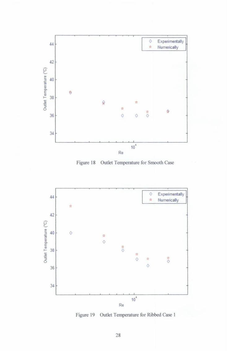
Figure 18 Outlet Temperatore for Smooth Case ...................................................... 28

Figure 19 Outlet Temperature for Ribbed Case 1 .................................................... 28

Figure 20 Outlet Temperature for Ribbed Case 2 .................................................... 29

Figure 21 Outlet Temperatore for Ribbed Case 3 .................................................... 29

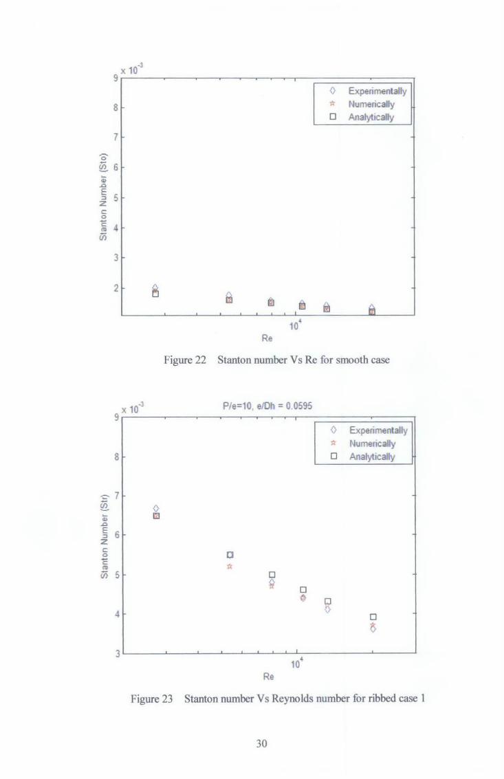
Figure 22 Stanton number V s Re for smooth case ................................................... 30

Figure 23 Stanton number Vs Reynolds number for ribbed case 1 ........................... 30

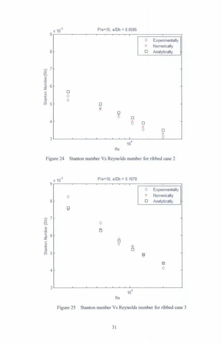
Figure 24 Stanton number V s Reynolds number for ribbed case 2 ........................... 31

Figure 25 Stanton number Vs Reynolds number for ribbed case 3 ........................... 31

Figure 26 Friction factor Vs Re for smooth case ...................................................... 32

Figure 27 Friction Factor Vs Re for ribbed Case !... ................................................ 32

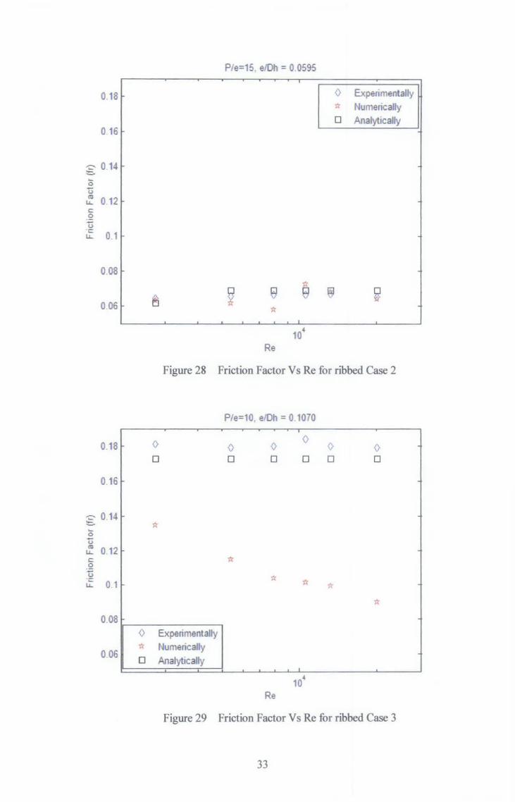
Figure 28 Friction Factor Vs Re for ribbed Case 2 ................................................... 33

Figure 29 Friction Factor Vs Re for ribbed Case 3 ................................................... 33

Figure 30 Heat transfer Enhancement for case 1 ....................................................... 3 5

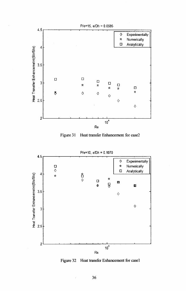
Figure 31 Heat transfer Enhancement for case2 ....................................................... 36

vi

Figure 32 Heat transfer Enhancement for case! ....................................................... 36

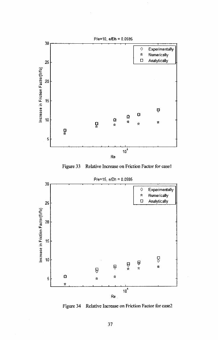
Figure 33 Relative Increase on Friction Factor for easel ......................................... 37

Figure 34 Relative Increase on Friction Factor for case2 ......................................... 37

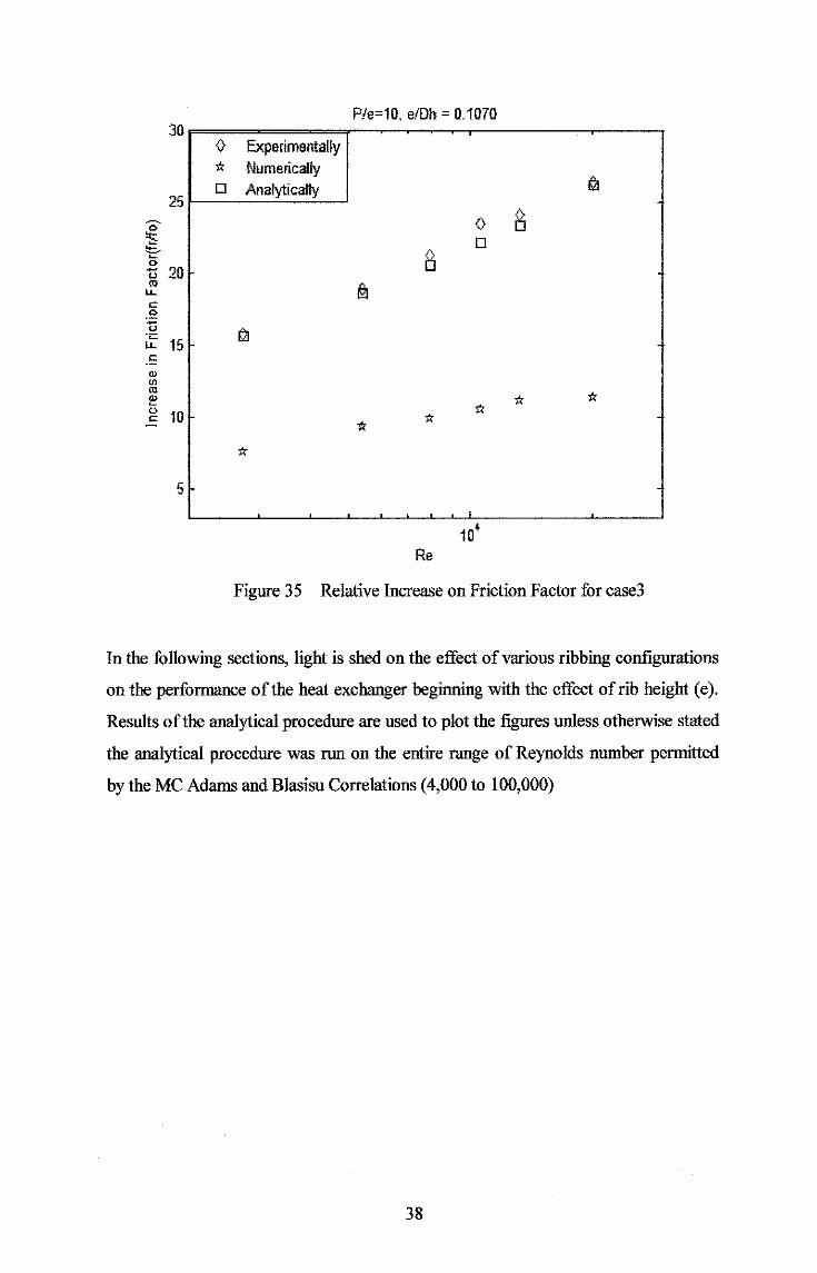
Figure 35 Relative Increase on Friction Factor for case3 ......................................... 38

Figure 36 Relative Changes in Friction Factor (fr/fo) Vs Reynolds Number ............ 39

Figure 37 Heat Transfer enhancement (str/sto) Vs Reynolds Number ..................... 39

Figure 38 Vortices generated by rib with e=0.0595 ................................................. 41

Figure 39 Vortices generated by rib with e=O. 765 ................................................... 41

Figure 40 Relative increase in friction factor for three different pitch sizes .............. 42

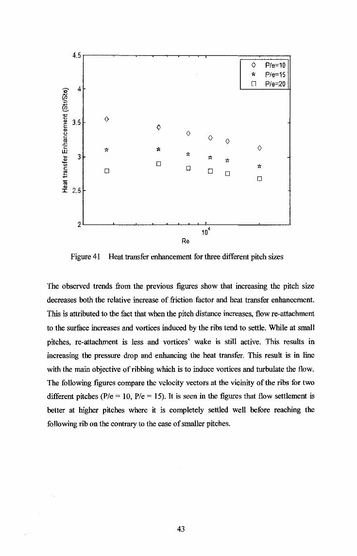
Figure 41 Heat transfer enhancement for three different pitch sizes ......................... 43

Figure 42 Vortices generated at P/e-1 0 .................................................................... 44

Figure 43 Vortices generated at P/e-15 .................................................................... 44

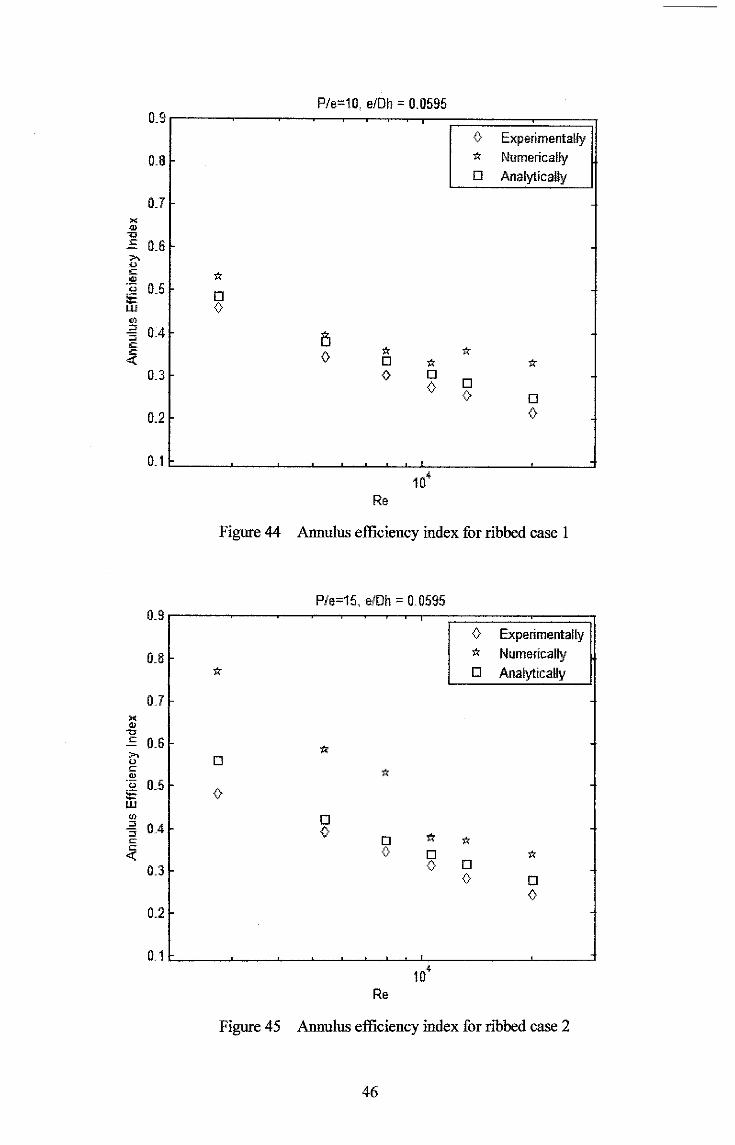
Figure 44 Annulus efficiency index for ribbed case 1 .............................................. 46

Figure 45 Annulus efficiency index for ribbed case 2 .............................................. 46

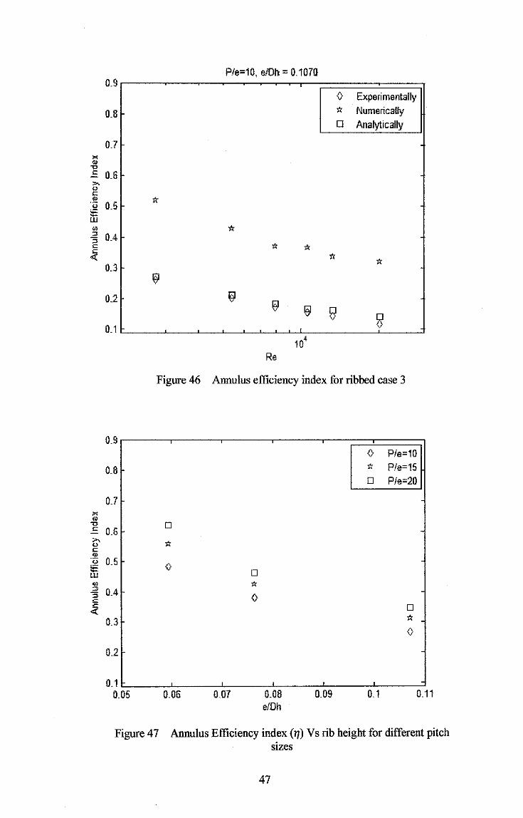
Figure 46 Annulus efficiency index for ribbed case 3 .............................................. 47

Figure 47 Annulus Efficiency index (71) Vs rib height for different pitch sizes ......... 47

Figure 48 Outlet Temperature Vs Reynolds number ................................................ 49

Figure 49 Stanton number Vs Reynolds number ...................................................... 49

Figure 50 Friction factor Vs Reynolds number ........................................................ 50

Figure 51 Annulus efficiency index Vs Reynolds number ....................................... 51

VII

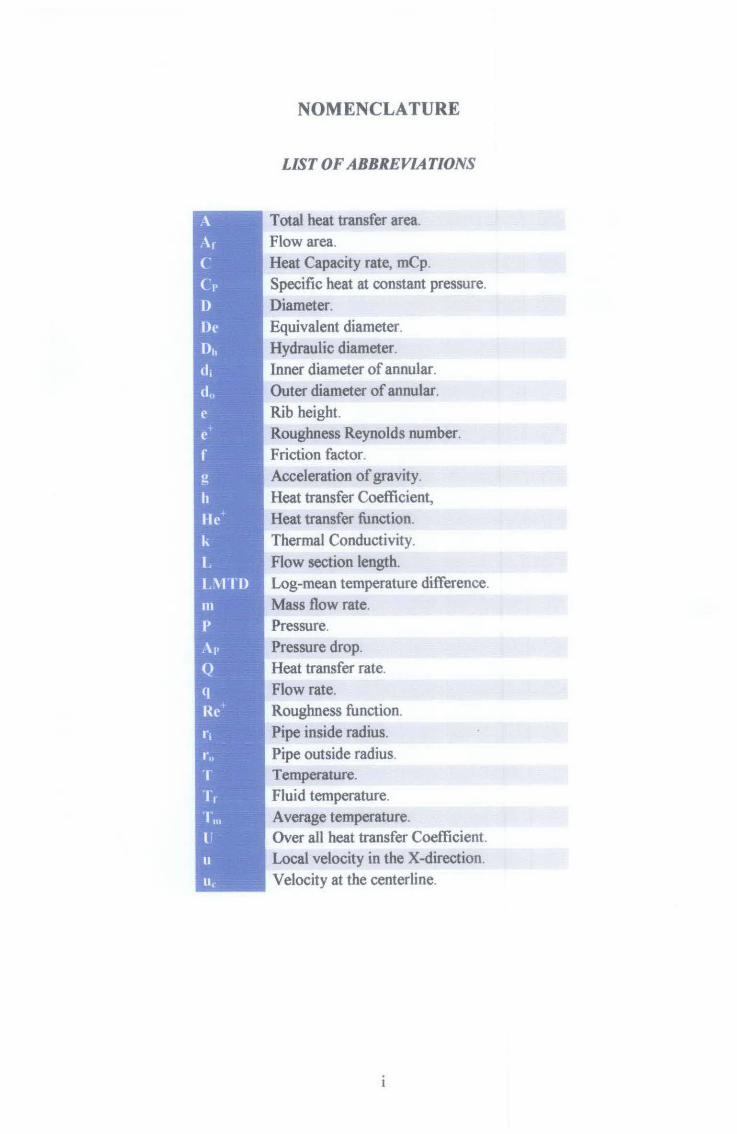
NOMENCLATURE

LIST OF ABBREVIATIONS

Total heat transfer area. Flow area. Heat Capacity rate, mCp. Specific heat at constant pressure. Diameter. Equivalent diameter. Hydraulic diameter. Inner diameter of annular. Outer diameter of annular. Rib height. Roughness Reynolds number. Friction factor. Acceleration of gravity. Heat transfer Coefficient, Heat transfer function. Thermal Conductivity. Flow section length. Log-mean temperature difference. Mass flow rate. Pressure. Pressure drop. Heat transfer rate. Flow rate. Roughness function. Pipe inside radius. Pipe outside radius. Temperature. Fluid temperature. Average temperature. Over all heat transfer Coefficient. Local velocity in the X -direction. Velocity at the centerline.

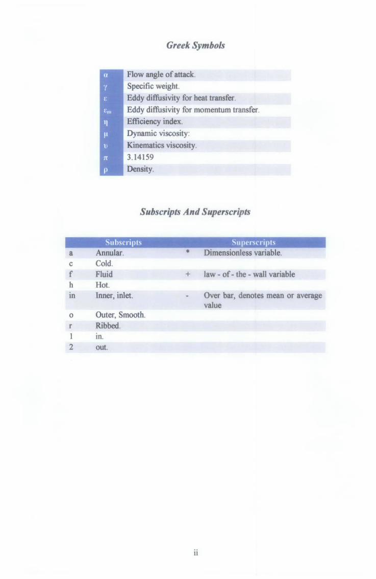
a c f h m

0

r 1 2

Greek Symbols

Flow angle of attack.

Specific weight. Eddy diffusivity for heat transfer. Eddy diffusivity for momentum transfer. Efficiency index. Dynamic viscosity: Kinematics viscosity. 3.14159

Density.

Subscripts And Superscripts

Subscripts Superscripts

Annular. • Dimensionless variable . Cold. Fluid + Jaw - of- the - wall variable Hot. Inner, inlet. Over bar, denotes mean or average

value Outer, Smooth. Ribbed. ln.

out.

11

1.1 BACKGROUND

CHAPTER I

INTRODUCTION

A heat exchanger is an equipment in which heat is transferred from a hot fluid to a

colder fluid. In most applications, the fluids do not mix but heat is transferred through

a separating wall which takes on a wide variety of geometries. Heat exchangers are

widely used in systems such as refineries, power plants, Oil Central Processing

Facilities (CPF) and many other systems

The increasing cost of energy in the past few years arouse the need for using more

efficient energy systems. This in turn encouraged researches in the field of

augmenting or intensifYing heat transfer in heat exchangers. Four techniques are

recognized for the study of heat transfer enhancement, these are:

i. Continuously Supplied Augmentative Stimulation. (Fluid Additives)

ii. Turbulence Promotion.(Ribbing .... etc)

iii. Extended Heat Transfer Surfaces. (Finned Tubes)

iv. Enhanced Heat Transfer Surfaces (Material Properties)

1.2 PROBLEM STATEMENT

The increasing cost of energy in the past years aroused the need for using more

efficient energy systems. This in turn encouraged researches in the field of

augmenting heat transfer in heat exchangers. Several techniques are recognized for

the study of heat transfer enhancement; out of which, ribbing is found to be a

powerful heat transfer enhancing tool. Yet, most of the work performed in this area

has thus far been mainly experimental with few numerical and analytical

investigations.

1.3 OBJECTIVES

i. To analytically simulate a ribbed double pipe heat exchanger.

ii. To numerically simulate a ribbed double pipe heat exchanger.

iii. To analyze the thermo fluid mechanisms

iv. To investigate different ribbing configurations

1.4 SCOPE OF STUDY

In this project, the effect of various parameters on the friction factor as well as

Stanton number is investigated. These parameters are: Reynolds number, rib height to

Hydraulic Diameter ratio (eiDJ,) and rib pitch to height ratio (P/e). The investigation

is curried out using analytical and numerical techniques whose results are compared

against previously obtained experimental data for validation.

1.4.1 Significance of the Study

Enhancing the performance of heat transfer media implies less heating energy to be

needed. This will improve the overall efficiency of a given plant reducing its

operating cost and ultimately, reducing the global costs of energy. Plants such as oil

processing facilities, power plants, refineries ... etc are all examples of plants that

extensively use heat transfer principles in their operation which need to enhance the

used heat transfer media

2

CHAPTER2

LITERATURE REVIEW

An early study of the effect of roughness on friction and velocity distribution was

experimentally performed by Nikuaradse [l] who is regarded as one of earliest

contributors in the field.

Webb et a! [2] in 1970 developed a number of correlations for heat transfer and

fiction factor for turbulent flow in tubes having repeated-rib. He also developed a

generalized understanding of the Stanton number and friction characteristics of

repeated.

An important concept used to evaluate the overall effect of ribbing on the flow at

different parameters was introduced by Webb [2]. This is the concept of annulus

efficiency index which is the relative increase in friction necessary to achieve the

desired heat transfer augmentation.

An interpretation for the heat transfer and pressure drop behavior in the presence of

turbulators/ roughness elopements was presented by Takase in 1996, a [3,a] when he

conducted an experimental and 2D/3D aualysis on ribbed-roughened annulus flow. It

attributes the heat transfer augmentation caused by the spacer rib to the increase of

axial velocity due to a reduction in the channel cross section in the presence of ribs

which promotes turbulence at earlier stages of the flow.

Later at the same year, Takase [3,b] developed a numerical technique for prediction

of augmented turbulent heat transfer in an annular fuel channel with repeated two­

dimensional square ribs in which a numerical model for predicting the Nussalt

number was built. This work is a continuation of the previous work presented above

of the same researcher. In this study an annular fuel channel with square repeated 2D

ribs model was experimentally analyzed. Resuhs of the experimental analysis were

compared against a numerical model consisting of five equations proposed to predict

the Nu for the flow. These equations were solved using FLUENT. The proposed

equations revealed matching results to the experimental ones.

3

In 1998 [4], Yildiz et al studied the effect of twisted strips on the heat transfer and

pressure drop in heat exchangers. They have conducted an experimental study on

double pipe heat exchangers with both parallel and counter flow cases. Experiments

for the previous cases were conducted on smooth and roughened pipe. Roughening

effect was achieved by placing twisted narrow, thin metallic strips at the inner pipe

surfuce. Reynolds's number in these experiments was in the range of3400-6900 and

the results have shown an increase in the heat transfer up to 100% at a cost of 130%

increase in the pressure drop. They have concluded that: The heat transfer rates in

double-pipe air cooling systems may be increased by up to 100% by placing twisted

strip turbulators inside the tubes. Moreover, further improvements in heat transfer

may be acquired with increasing pitch size. Turbulators cause a considerable increase

in pressure drop, but the heat equivalent of this energy loss is negligible in

comparison with the heat gained by the turbulators.

In 1999 [5], Braun et al performed experimental and numerical investigation on

turbulent heat transfer in a channel with periodically arranged rib roughness elements.

The experiments were carried out on a Reynolds's number of 6000. The numerical

analysis was carried out nsing Large Eddy Simulation (LES). The results obtained

from this study has shown that even at the eighth periodic roughness element,

turbulent flow conditions were not developed which is mainly attributed to the fact

that the height of the element used in the study was not large enough to produce the

anticipated effect.

Another study was carried out in the year 1999 [6] by Al-Habeeb, on the effect of

ribbing on the parallel flow of double pipe heat exchangers. The study which was

conducted experimentally investigated two main cases, when hot flow is at the

annulus and when the cold flow is at the annulus. Reynolds's number used was in the

range of(l0000-72000) for the pipe flow and of (2600-20000) for the annular flow

for the frrst case and for the second case ranges of (12000-70000) and ( 4500-17000)

were used for the pipe and the aunulus respectively. The results obtained from this

study show that when the hot flow is inside the pipe, heat transfer enhancement of

4.26 was achieved while when the hot flow is in the annulus, enhancement of up to

4.4 was achieved.

In 2007 [7], Hact et al studied the effect of variable fin inclination angle on the

thermal behavior of a plate fin-tube heat exchanger. The study was performed

4

numerically using a 3-D model using GAMBIT software to create the model and

produce the meshing while FLUENT software was used to perform the numerical

analysis. The analysis was performed on a steady state, laminar flow with fin angles

varying from 0° to 30° with an increment of 5°. Results from this work shows that

heat transfer enhancement and effectiveness improvement were optimum at

inclination angle of 30° where heat transfer improvement was recorded to be l 05.24%

while accompanying pressure drop was found negligible.

In 2008 [8], Al-Kayiem and AI-Habeeb conducted a numerical study on the effect of

various ribbing configurations on the heat transfer. The study aimed to compare the

experimental results obtained in number [6] with the numerical results. The study

revealed good agreement between the experimental work and the numerical

correlations used

In 2008 [9], Ozxeyhan et al investigated numerically the heat transfer enhancement in

a tube using circular rings separated from the wall. This study differs from other

studies in the field in that the ribs here were not attached to the wall so that heat

transfer enhancement is solely due to disturbing of the laminar sub layer. The study

was carried out using FLUENT code and it was on a range of Reynolds number of

(4400-43000). Results from this study shown that heat transfer enhancement

increases with the pitch of the ribs.

5

CHAPTER3

METHODOLOGY

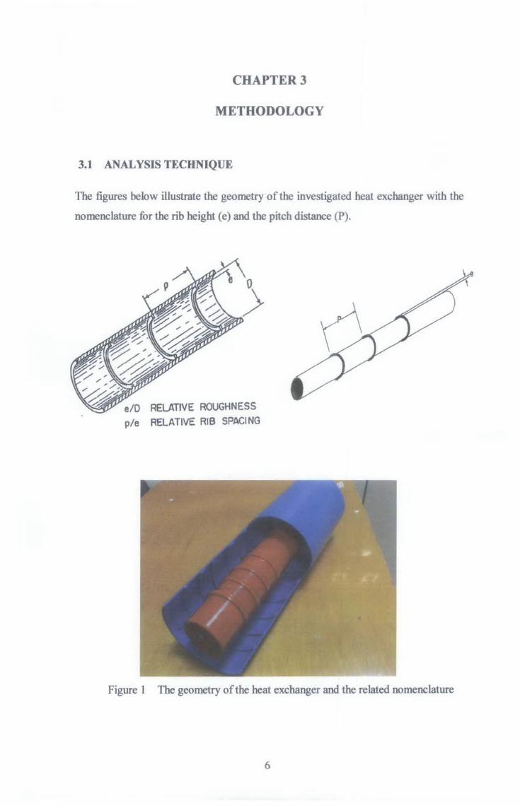
3.1 ANALYSIS TECHNIQUE

The figures below illustrate the geometry of the investigated heat exchanger with the

nomenclature for the rib height (e) and the pitch distance (P).

RELATIVE ROUGHNESS p/e RELATIVE RIB SPACING

Figure 1 The geometry of the heat exchanger and the related nomenclature

6

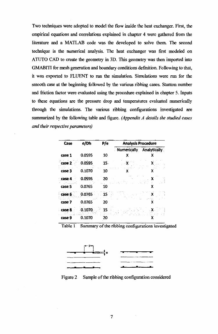
Two techniques were adopted to model the flow inside the heat exchanger. First, the

empirical equations and correlations explained in chapter 4 were gathered from the

literature and a MATLAB code was the developed to solve them. The second

technique is the numerical analysis. The heat exchanger was first modeled on

ATUTO CAD to create the geometry in 3D. This geometry was then imported into

GMABITI for mesh generation and boundary conditions definition. Following to that,

it was exported to FLUENT to run the simulation. Simulations were run for the

smooth case at the beginning fullowed by the various ribbing cases. Stanton number

and friction factor were evaluated using the procedure explained in chapter 5. Inputs

to these equations are the pressure drop and temperatures evaluated numerically

through the simulations. The various ribbing configurations investigated are

suunuarized by the following table and figure. (Appendix A details the studied cases

and their respective parameters)

case e/Dh P/e Analysis Procedure

Numerically Analytically case 1 0.0595 10 X X

case2 0.0595 15 X X

case3 0.1070 10 X X

case4 0.0595 20 X

caseS 0.0765 10 X

case6 0.0765 15 X

case7 0.0765 20 X

case a 0.1070 15 X

case9 0.1070 20 X

Table I Summary of the ribbing configurations investigated

•

Figure 2 Sample of the ribbing configuration considered

7

3.2 TOOLS AND SOFTW ARES

All simulations and MATLAB analysis were run on a computer with the following

specifications:

• Processor

• RAM

: Dual Core, 2.0 GHz

:2GB

A number of softwres were used in the current analysis as explained in the previous

sections. A list of all softwares is given below:

1. AUTOCAD

11. GAMBIT

iii. FLUNET

IV. MATLAB

3.3 FLOW CHARTS

The flowcharts in the following pages illustrate the methodology adopted for both the

analytical and numerical procedures.

8

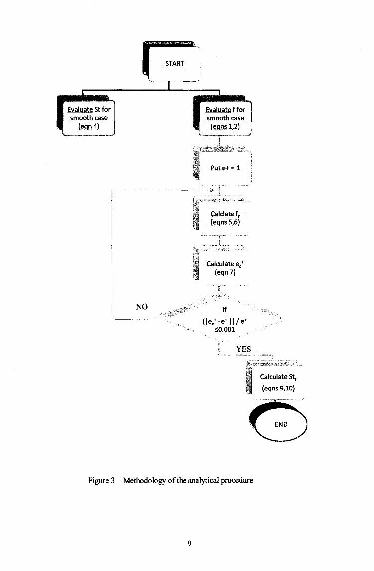
Evaluate St for smooth case

(egn4)

NO

START

Evaluate f for smooth case

(ggns 1,2)

Pute+ = 1

Calclatef, (eqns 5,6)

Calculate e; (eqn 7)

if

(Je:-e• J)fe• S0.001

YES

Figure 3 Methodology of the analytical procedure

9

Calculate St,

(eqns 9,10)

- ~ - -

Develop geometry on

AUTOCAD

Mesh geometry on GAMBIT

Run Simulation on FLUENT,

obtain /l.P and ~

---~--·---· -r~"'

~--~-. ---

Results match experiment?

YES

Figure 4 Methodology of the CFD procedure

10

NO

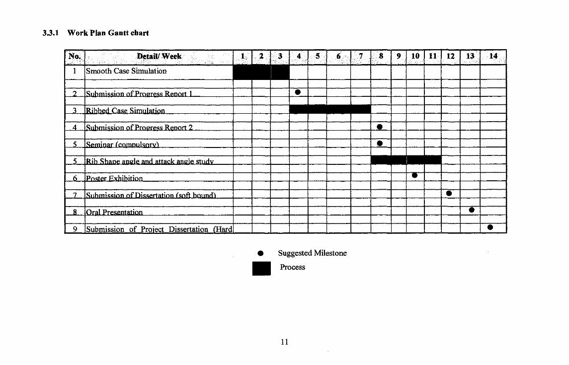
3.3.1 Work Plan Gantt chart

No.

1

2

3

4

_5

'i

6

7

8

9

·. :O~tail/ Week ..... 5 6 .

. . · .

Smooth Case Simulation

.. '»~n~ri 1 •

IR ihh .. t{ CasP. · ·i~n

I" . . 1 ot .n :2

IRih '""""1" Rnn : <malA «tnrlv

ln. ...

· · 1ofn· . l(«nfl'

I Oral

Submission of Proiect Dissertation /Hard

e Suggested Milestone

Process

11

. ·' .s 9 10 11 12 13 . 14 ...

• •

• •

• •

CHAPTER4

ANALYTICAL ANALYSIS

4.1 FRICTION FACTOR FOR SMOOTH CASES, f

Two correlations were used to evaluate the friction factor wherein the values are

selected with correspondence to the Re value. These correlations are as follows:

• Blasius correlation (Kakac [1 0]):

• Drew, Koo and McAdams correlation (Kakac [1 0]):

f=0.0014+0.125.Re-n32 4x104 sRes106 (2)

The previous correlations evaluate the friction factor as a function of Reynolds

number only.

4.2 THE CONVECTIVE HEAT TRANSFER FOR NON-RIBBED ANNULUS

CASES, St:

The same equations mentioned in section 3.1.3 are used, they repeated below:

Nu = h,D = 0.023Re0·8 Pr"

k

and the exponent, n has values of:

n = {0.4 for heating 0.3 forcooling

(3)

St= Nu (4) RePr

12

4.3 FRICTION FACTOR FOR RIBBED ANNULUS CASES, fr:

By combining the velocity defect law for pipe flow with the law of the wall,

Nikuradse [1 ], developed the "friction similarity law" for sand grain roughness. This

can be assumed to hold for the entire cross section of the flow. To satisry the ribbed

annulus flow, the average surfuce roughness, e is replaced by the rib height, e. The

Roughness function, Re + is obtained as:

where, the roughness Reynolds number, e + is:

(6)

Han [11] recommended a correlation for the friction factor for turbulent flow between

parallel plates with repeated-rib roughness by taking into account the geometrically

non similar roughness parameters ofP/e, rib shape, ll> and the angle of attack, a, as:

where the exponents m, n are given as follows:

m=-0.4

m=O

n = -0.13

f )'·" n=O.S\_9~

if

if

if

if

e+ < 35

e+:::: 35

P/e < 10

P/e:::: 10

(7)

Equations, 16, 17, and 18 were solved iteratively by using initial guess of e + = 1 and

substituting into equation 17. Re + is substituted for from equation 18. Iterations were

performed until residues fell below 0.001.

4.4 HEAT TRANSFER FOR RIBBED ANNULUS CASE, Str:

Han et a!. [11] and Webb et al. (12] proposed a formula that applies the heat and

momentum transfer analogy known as" Heat Transfer Similarity Law" as follows:

13

( /, ) 1 2St R + _ u +f + P ) ( ~ rl + e - ne \e ' r

(8)

where, He+, Re+ and f, are known,- f,. is calculated as in subsection 3.2.3 above-,

then Stanton number in the ribbed flow could be evaluated as:

(9)

Values of He+ can be found using the following correlation recommended by Webb

et al. [12]

He+ = 4.5 · ~+ J28 (Pr )057 (10)

14

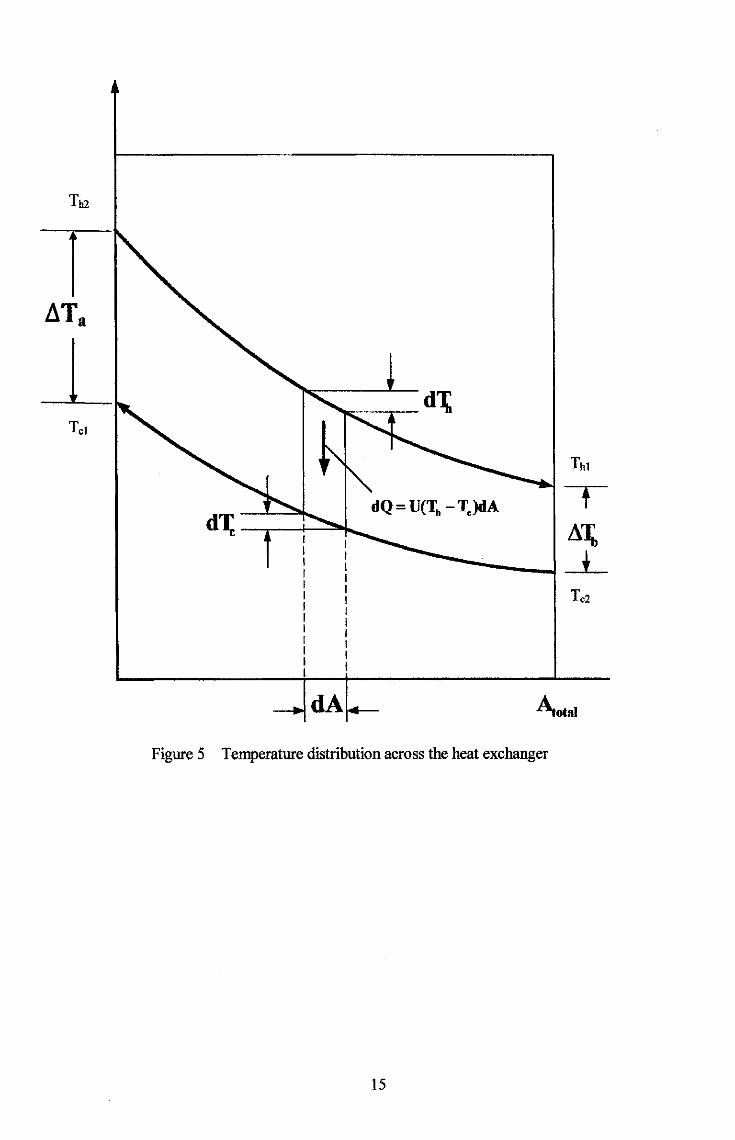
Tb2

dA .A.otal

Figure 5 Temperature distribution across the heat exchanger

15

CHAPTERS

NUMERICAL ANALYSIS

5.1 OVERALL HEAT TRANSFER

The total heat transferred from the hot fluid in the pipe to the cold fluid in the annulus

is given by the relation:

Qh = mh Cph (Thl- Th2) = Qe = me Cpe (Te2- Tel) (11)

The total heat transferred is also given using the overall heat transfer coefficient as

follows:

Where:

pipe;

Q = UoAilTm (12)

A is the total heat transfer area- the outer surfuce of the pipe in this case -

Uo is the overall heat transfer coefficient based on the outer surfuce area of the

1 u 0 = ::-------,----,---;;-:-[ (r~hi) + (rm) Ln~~ + h~]

(13)

ll T m is the Jog mean temperature difference across the pipe; if subscripts a, b

indicate the pipe inlet and outlets respectively, then ll T m is given by:

llTb- llTa llTm = ----.=-­Ln IJ.Tb

IJ.Ta

5.2 FRICTION FACTOR, f:

(14)

In fully developed flow in closed conduits, either laminar or turbulent, the pressure

drop varies with inertia force parameters, shear force parameters and the surface

conditions as:

16

(15)

Where, e is the absolute roughness of the conduit surface having dimensions of

length. J.l and p are the fluid viscosity and density, respectively and Urn is the mean

velocity. Using dimensional analysis and adopting the hydraulic diameter criteria, Dh

instead of the pipe diameter, D, getting the known Darcy Weisbach equation from

which the friction factor ,j in the annular flow is:

{16 )

Where, the hydraulic diameter for the annulus is:

_ {:)d;-dn Dh- d.-d;

ml. + ml; (17)

The outlet pressure is evaluated either from the experiment or from the simulation

results. Inlet pressure on the other hand is evaluated knowing that pumping power

used for the experiment was 5 hp, with efficiency of 65%. The pressure is then

calculated using the formula:

q Pi 1'/ =­p

Where 11 is the pumping efficiency;

Q is the fluid flow rate;

Pi is the inlet pressure;

P is the pumping power in KW.

5.3 THE CONVECTIVE HEAT TRANSFER, St:

(18)

The coefficient of convective heat transfer, h is a function of many variables such as

the geometry of the flow passage, the surface roughness, the flow direction and

velocity, temperatures of the fluid and the surface and the fluid properties (density,

viscosity, heat capacity and the thermal conductivity). The differential equations of

convection are of the most difficult class and the empirical treatment is not entirely

satisfactory, but yields adequate results. Accordingly, treatment of the above set of

17

variables by dimensional analysis method has led to number of correlations in the

form of:

Nu = Nu(Re, Pr) (19)

For fully developed turbulent flow in pipes with e ID < 0.001, the following

correlation is recommended by Dittus and Boelter as mentioned by [10]:

hD os Nu = -'-= 0.023Re · Pr"

k

and the exponent, n has values of:

n={0.4 0.3

for heating

for cooling

(20)

The equation is used in the present annulus flow by using Dh instead of D. The

physical properties were evaluated at the mean bulk temperature. Accordingly,

Nu St=-­

RePr

5.4 GEOMETRY CREATION

(2~

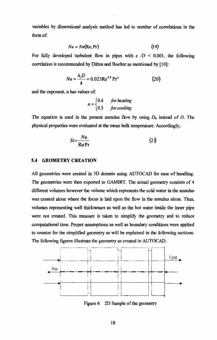
All geometries were created in 3D domain using AUTOCAD fur ease of handling.

The geometries were then exported to GAMBIT. The actual geometry consists of 4

different volumes however the volume which represents the cold water in the annulus

was created alone where the focus is laid upon the flow in the annulus alone. Thus,

volumes representing wall thicknesses as well as the hot water inside the inner pipe

were not created. This measure is taken to simplifY the geometry and to reduce

computational time. Proper assumptions as well as boundary conditions were applied

to counter for the simplified geometry as will be explained in the following sections.

The following figures illustrate the geometry as created in AUTOCAD.

1- 1-

Cold

Hot

Figure 6 2D Sample of the geometry

18

Figure 7 A 3D sample of the geometry

5.5 MESHGENERATION

The geometry was meshed using the volume meshing tooL Only one element type

was sucessfully applied that is the Tetrahedral type. Errors were received when

attmpteing to use any other element type. This is believed to be a result of the

complex interior of the geometry due to the presence of the ribs. Interval size used is

0.55 units and the total number of elements created is 293,104 elments.

Figure 8 Sample of the meshed geometry

5.5.1 Boundary Conditions

In all of the investigated cases, the pressure at outlets is unknown and therefore it is

not possible to use a boundary condition which uses pressure as a user input. Hence,

Velocity inlet is used for the flow inlets in the annulus and outflow is used for the

outlets. The outer walls were set as walls with no thermal conditions.

19

The inner wall separating annulus from inner pipe contains a thermal boundary

conditioJL This boundary condition is either to be set by the user or to be left to the

simulation to evaluate. In the latter case, other inputs are required such as outlet

pressure which is unknown. Due to the several unknowns in the problem, an

assumption was made that the heat flows uniformly from the hot pipe to the cold

annulus throughout the heat transfer area. With that assumption, the heat flux is

calculated from the experimental data using the formula below:

mcpiJT if> = ---":--­

A

The calculated value is used as a thermal condition input to the simulation. Now,

since the heat flux value is predetermined, there is no needed for the solver to

perform any calculations on the inner pipe and since it is the annulus in which the

study is interested, the inner pipe geometry was not created. This would save the

calculation resources and reduce the simulation time,

5.6 SIMULATION SET UP

All simulations were run on FLUENT 6.2 using the 3D Double Precision mode

(3DPP). The following sub section illustrates the turbulence model employed and the

relevant equations.

5.6.1 The Turbulence Model

Reynolds averaging of the Navier-Stocks equations was employed to solve the

turbulent model wherein, the instantaneous (exact) Navier-Stokes equations are

decomposed into the mean (ensemble-averaged or time-averaged) and fluctuating

components in the general form for a given quantity ~:

if> = if+ if>' (22)

The Navier-Stocks equations in the averaged form can be written as:

Up iJ , , - + -(fi!Lj = () (23) Ot i!:r1 •

20

The model used is the RNG k-& model which is derived using the statistical technique

(called renormalization group theory) and contains an extra term in its & equation

which improves its accuracy. The transport equations (K-&) are as follows:

D,,,, 0,_,_. U(--- Uk) (,' -, 1. -. -:-•.JW_! + -;-:"'·Jln'll;) = ~ ilk/leff-;-:" + 'k + (,b- j)f- M + !Jk (25) dt d.! i iJ.! j dJ j

and

The main difference between the RNG and standard k-& models lies in the additional

term in the 8 equation given by

R _ L~p1J3(1-I)/I)o) E"

'- 3 1 + 3q k (27)

Where

"'' 1 _, ·2~· J {-I (-'l''l !J=·-'"'fE.lJo='>.·-•-',.:'= -·' ~-

The equations' constants were left at their default values set by FLUENT 6.2 as

follows: Ctc = 1:42; Cz. = 1:68. For the turbulence intensity, Versteeg and

Malalasekera [13] recommended using values of no greater than 10% fur high

turbulent flow while using values between 1-5% for less turbulent flow. Based on this

the turbulence intensity was set to 3% for the smooth case and 10% for the ribbed

cases.

Versteeg and Malalasekera [13] also recommended the use of QUICK descretisation

scheme (Quadratic Upstream Interpolation for Convective Kinetics) yet, the QUICK

scheme is not available under FLUENT 6.2 and therefore the second order upwind

discretisation was applied to all equations instead.

Defuuh convergence criteria were used where it is set at 0.001 for all equations

except for the energy equation which is set to 10-6. Convergence was reported after

100 to 200 iterations. A sample of the residuals is shown below.

21

(26)

Residuals ontinuity -velocity

-y-velocjty --z-ve1oc1ty

energy -k

A il n

1 e-t01

1e~oo

1e-01

1e-02

1e-03

1e-04

1e-05

le-06

le-07 0

I.

---25 50 75 100 125 150 175 200 225

Iterations Figure 9 Sample of Residuals

0 10 20 3:) 40 5) 00 70 a) 9) 100

Iterations

Figure 10 Sample of residuals

22

5.6.2 Grid Independency Check

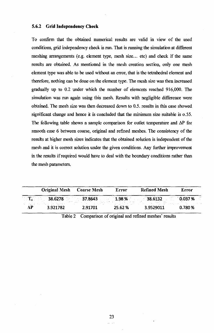
To confirm that the obtained numerical results are valid in view of the used

conditions, grid independency check is run. That is running the simulation at different

meshing arrangements (e.g. element type, mesh size ... etc) and check if the same

results are obtained. As mentioned in the mesh creation section, only one mesh

element type was able to be used without an error, that is the tetrahedral element and

therefore, nothing can be done on the element type. The mesh size was then increased

gradually up to 0.2 under which the number of elements reached 916,000. The

simulation was run again using this mesh. Results with negligible difference were

obtained. The mesh size was then decreased down to 0.5. results in this case showed

significant change and hence it is concluded that the minimum size suitable is o.SS.

The following table shows a sample comparison for outlet temperature and LV> for

smooth case 6 between coarse, original and refined meshes. The consistency of the

results at higher mesh sizes indicates that the obtained solution is independent of the

mesh and it is correct solution under the given conditions. Any further improvement

in the results if required would have to deal with the boundary conditions rather than

the mesh parameters.

AP

Original Mesh Coarse Mesh

38.6278

3.921782

37.8643

2.91701

Error

1.9.8%

25.62%

Refined Mesh

38.6132

3.9529011

Table 2 Comparison of original and refined meshes' results

23

Error

0.037%

0.780%

CHAPTER6

RESULTS AND DISCUSSION

6.1 SIMULATION RESULTS

Six different Reynolds numbers were investigated in all ribbed cases as well as the

smooth case ranging from 2,000 to 20,000. These values were obtained from the

experimental data by AJ-Habeeb [5].

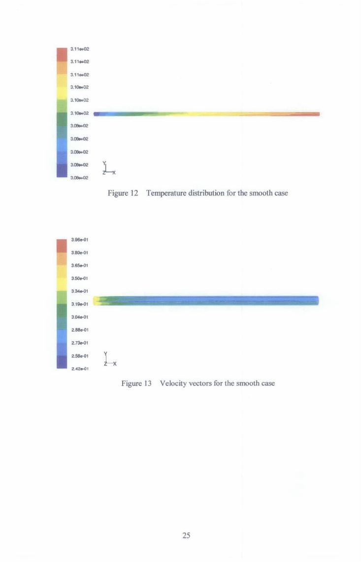
The following figures illustrate various aspects of the flow properties for the smooth

case and sample of the ribbed cases. These aspects include pressure variation across

the flow, temperature distribution and the velocity vectors.

3.71»01

·9.00..00

· 1.ee..o1

·2.7s..o1

·3.74 .. 01

·4.ee..01

·6.831tt01

·6.67..o1

-7.61 .. 01

·8.40..01 ~ ·9.40..01

Figure 11 Static pressure profile for the smooth case

24

3.11 .. 02

3.11..o2

3.11..o2

3.10..02

3.10&t02

3.10..02

3.CS..02

3.cs..02

3.CS..02

3.cs..02 ~ 3.cs..02

Figure 12 Temperature distribution for the smooth case

3.96e-01

3.so.Hit

3.SS.01

3.504Hlt

3 34.Hlt

3.19.01

3.04&{)1

2.88ri1

2.73e-OI

2.58e-01 L 2.42e-01

Figure 13 Velocity vectors for the smooth case

25

1. 15&+02

3.660+01

-4.24&+01

-1 21&+02

-2.00o+02

-2.796+02 (

-3.58e+02

-4.37&+02

-5.1~

-5.~

-6.74H02

3.10..02

3.10..02

3.te.to2

3.CS...02

11· ~-

L Figure 14 Sample pressure profile for ribbed cases

Figure 15 Sample temperature profile for ribbed cases

26

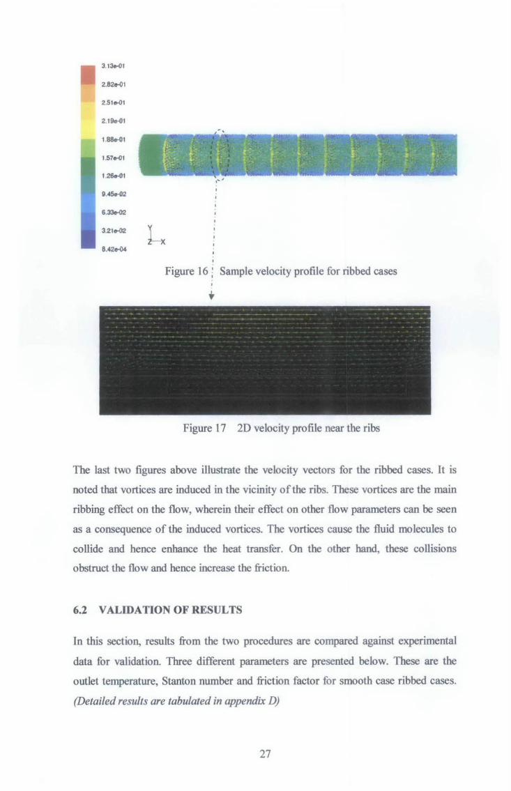
31~1

2.82..01

2 .51..01

2.1~1

.-·-' > I

f:· L I. • t l . 1.

~ t: L t' l: ' • t-~- . ~ f· ••

.c:··- ~ • ,; .· t··,· f r r i. f t . . . •· l

Figure 16 ; Sample velocity profile for ribbed cases

Figure 17 2D velocity profile near the ribs

The last two figures above illustrate the velocity vectors for the ribbed cases. It is

noted that vortices are induced in the vicinity of the ribs. These vortices are the main

ribbing effect on the flow, wherein their effect on other flow parameters can be seen

as a consequence of the induced vortices. The vortices cause the fluid molecules to

collide and hence enhance the heat transfer. On the other hand, these collisions

obstruct the flow and hence increase the friction.

6.2 VALIDATION OF RESULTS

In this section, results from the two procedures are compared against experimental

data for validation. Three different parameters are presented below. These are the

outlet temperature, Stanton number and friction factor for smooth case ribbed cases.

(Detailed results are tabulated in appendix D)

27

44

42

-(.) t..... Q)

:; 40 1ii ... Q)

a.. E Q)

t- 38 .N :; 0

36

34

44

42 ......... () t..... Q)

:; 40 -(g

lii a.. E Q)

t- 38 .]! 'S 0

36

34

* l.'{

0 0

Re

lt 0

0 Experimentally

* Numerically

Figure 18 Outlet Temperature for Smooth Case

0 Experimentally .... Numerically

lt

0

* 0

* 0 lt .... 0

0

Re

Figure 19 Outlet Temperature for Ribbed Case 1

28

.

44

42 ...... E

Cl)

5 40 (ii Cii 0. E Cl)

...... 36 j :; 0

36

34

44

42

-p -Cl) ._ 40 ::J -co

G; 0. E G)

...... 38 ]! :; 0

36

34

0

* 0

0

0

Re

0

1 0~

Experimentally Numerically

Figure 20 Outlet Temperature for Ribbed Case 2

* 0

~

Re

* 0 *

0 Experimentally

* Numerically

0

Figure 21 Outlet Temperature for Ribbed Case 3

29

8

7

3

2

Re

0 Experimentally l'l Numerically

0 Analytically

Figure 22 Stanton number V s Re for smooth case

10·3 P/e=10, e/Dh = 0.0595 9 rx----~--~~~~~~~--~====~====~

8

"C' 7 §. 0 Q; rn ..0

E 6 :J z c 0

c (ll

V5 5

4

3

Figure 23

0

0 9 0

~

104

Re

0 Experimentally

Numerically

0 Analytically

0 0

0 0

Stanton number Vs Reynolds number for ribbed case 1

30

8

4

0 0 tc

P/e=15, e/Oh = 0 0595

0 ~

[;J

0 0

0

0 Experimentally \"<" Numerically 0 Analytically

0 .. 0 0

~ 10

4 3 L-----~--~--~--~~~~-L----------~----~

Re

Figure 24 Stanton number Vs Reynolds number for ribbed case 2

9 X 10.3 P/e=10, e/Oh = 0 1070

0 Expenmentally

0 Numencally 8 0 Analytically

~

"1::'7 ~ 0 ..... Q)

b ..a E 6 ::I z c 0

~ -c: (U

(i) 5 ~

rJ

4 0

3 L-----~--~--~--~~~~-L----------~----~

10~ Re

Figure 25 Stanton number Vs Reynolds number for ribbed case 3

31

0.18 <> Experimentally ~ Numerically

0 16 D Analytically

0 14

,....... g_ 0.12 0 u

0.1 Ill La.. c: 0

u 0 08 ~

La..

0.06

004

0 02 'l'r

0 0 ~ A n

104

Re

Figure 26 Friction factor Vs Re for smooth case

P/e=10, e/Dh = 0.0595

0 18 <> Experimentall:t ~ Numerically D Analytically

0 16

-;:::- 014 :::::. ... 0

u Ill 0 12 La.. c:

.5:! u ·;::

0.1 ~ La..

tl ~

E3 0 § (3 0 0 08 ll

* 0 06

I

104

Re

Figure 27 Friction Factor V s Re for ribbed Case 1

32

0.18

0.16

0 014 ::::. 0 u 10 0 12 ...... c e 0 .....

0 1 u.

0 08

0.06

0 18

0.16

0 014 :::::::.. ..... 0

u 10

0.12 u. c .e .g

0 1 u.

0 08 0 ~

0 06 0

P/e=15, e!Dh = 0.0595

~

Re

0 Experimentally Numerically

0 Analytically

Figure 28 Friction Factor Vs Re for ribbed Case 2

P/e=10, efDh = 0.1070

0 0

0 " v 0 0 0 0 0 0

t<-*

Experimentally Numerically Analyttcally

104

Re

Figure 29 Friction Factor V s Re for ribbed Case 3

33

The temperature results reveal good agreement between the numerical and the

experimental data. This validates the thermal boundary condition assumption

mentioned in section 5.3 .1. It is noted however on the smooth case figure that greater

discrepancy was sustained for the mid range values. The experimental data for this

range showed constant value for the Reynolds numbers which is believed to be an

error in reporting the experiment data where it is expected that temperature should

vary as Reynolds number changes.

Stanton number which is a function of the outlet temperature showed good agreement

too, both numerically and analytically. From these two remarks a conclusion is drawn

that heat transfer was successfully modeled analytically and numerically.

Considering the friction factor for the smooth case, it is noted that generally Blasius

correlation is more conservative than Me Adams'. However Me Adams' is closer to

experimental results. The two correlations tend to become identical at high Reynolds

numbers. For the ribbed cases, analytical results show good agreement with the

experimental data which validates the used procedure to analytically model the

friction factor. Numerical data on the other hand exhibit greater discrepancy specially

for the third case. This may be attributed to errors in pressure conditions used during

the simulation. However with the absence of the pressure data for the experiment it is

not possible to confirm the source of discrepancy.

The general trend observed in both friction fuctor and Stanton number figure is that as

Reynolds number increases, both friction factor and Stanton number decrease. The

decrease in the friction fuctor can be explained by considering the fact that Reynolds

number, of which both friction factor and Stanton number are functions, is the ratio of

inertia forces to frictional forces expressed by the fluid viscosity. At high Reynolds

numbers velocity increases and eventually, inertia forces outweigh frictional forces.

The following figures illustrate the relative increase in both Stanton number (heat

transfer enhancement) and the friction factor which are the ratio of Stanton number

and the friction factor for ribbed cases to the smooth case respectively. These two

parameters are usually the main parameters offocus when assessing the ribbing effect

rather than considering their absolute values. As can be seen, generally, both

34

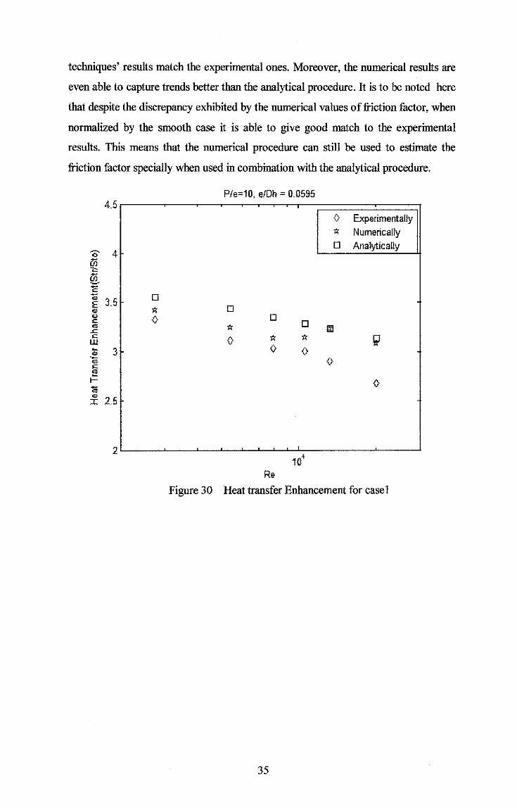
techniques' results match the experimental ones. Moreover, the numerical results are

even able to capture trends better than the analytical procedure. It is to be noted here

that despite the discrepancy exhibited by the numerical values of friction factor, when

normalized by the smooth case it is able to give good match to the experimental

results. This means that the numerical procedure can still be used to estimate the

friction factor specially when used in combination with the analytical procedure.

P.le=10, eiDh = 0_0595 4_5

0 Experimentally

"' Numerically 0 Anal}'tica!ly

0' 4 Ui "' @. 'E -;;;

3_5 0 E 0 ., "' 0 0 0 <:: 0 .. "' m .c <::

0 "' "' w ~ 3 0 0 ., - 0 ., <:: ~ I--;;; .,

2.5 :r:

Re

Figure 30 Heat transfer Enhancement for easel

35

P!e=15, e/Dh = 0.0595 4.5

<> Experimentally

"' Numerically 0 Analytically

0' 4 i/5 "' -(/) ~

c ;;;

3.5 c L .. " "' ..

..<: c

0 w 0 ;;; 3 0

0 - "' "' 0 ., "' "' "' D .. - <> <> "' 1-.. <> ..

2.5 <> I

Re

Figure 31 Heat transfer Enhancement for case2

P/e=10, e/Dh = 0.1070 4.5

{} Experimentally 0 "' Numerically <> 0 Analytically

~ 4 5 0

"' i/5 "' <> 0 "' i/5 9

m ~ >$ "E' -"' 3.5 E {} "' <.>

" "' -"'-c w :;; 3 -"' cc "' ~ .. "' 2.5 -I

Re

Figure 32 Heat transfer Enhancement for easel

36

P/e=10, e/011 = 0_0595 30

0 Experimentally

* Numerically

25 D Analytically

'0 'S ""-~ 0 - 20 (J

"' '-'-

" _e ti -;::

15 '-'-£ .,

~ ., "' .,

r:J 01 ~ (J

10 Q -= * * * * 01 * 5

104

Re

Figure 33 Relative Increase on Friction Factor for case I

P!e=15, e/Dh = 0_0595 30

0 Experimentally

* Numerically

25 D Analytically

'0 'S "'-0 ti 20 "' '-'-" 0 -.;:; (J

~ 15 _!:; ., ., "' E

~ (J

10 "' @ @ @

8 * * * 5 Q

* * *

104

Re

Figure 34 Relative Increase on Friction Factor for case2

37

5

'

Re

Figure 35 Relative Increase on Friction Factor for case3

In the following sections, light is shed on the effect of various ribbing configurations

on the performance of the heat exchanger beginning with the effect of rib height (e).

Results of the analytical procedure are used to plot the figures unless otherwise stated

the analytical procedure was run on the entire range of Reynolds number permitted

by the MC Adams and Blasisu Correlations ( 4,000 to 1 00,000)

38

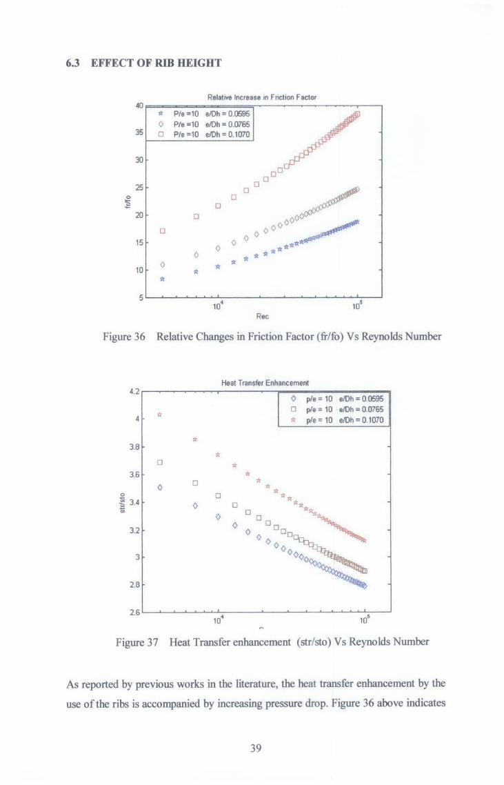
6.3 EFFECT OF RIB HEIGHT

Relative Increase in F net ion Factor 40

~ P/e =10 e/Oh = 0.0595 P/e :;::10 e/Oh :;:: 0.0765

35 0 P/e =10 e/Dh = 0.1070

30

oo

25 oo

/ 0 0 0 'S 0 ....

20 0 oooo~ 0 ooo

15 0 0 0

,:rllr~ 0 ,:rlll',:r

0 It-R: R

0 R: ~

10 R ,:r

5 10

4 10

6

Rec

Figure 36 Relative Changes in Friction Factor (fr/fo) Vs Reynolds Number

4.2

4 ~

:It

3.8

* 0

3.6

0 0

0

~ 3.4 ;;;

0

0 0

3.2

3

2.8

2.6

Heat Transfer Enhancement

*

0

0

R: R:

* *

0 pie = 10 e/Oh = 0.0595 D pie = 10 8/0h = 0.0765

pie= 10 e/Oh = 0.1070

*:~~:

**

:: 0 000~ oo

ooooo~

Figure 37 Heat Transfer enhancement (str/sto) Vs Reynolds Number

As reported by previous works in the literature, the heat transfer enhancement by the

use of the ribs is accompanied by increasing pressure drop. Figure 36 above indicates

39

that the increase of friction fuctor and hence pressure drop are higher at high

Reynolds numbers. It also indicates that as the rib height increases, so does the

increase in pressure drop.

Heat transfer enhancement exhibits an opposite trend where the heat transfer

enhancement drops as Reynolds number increases. Yet the trend with rib is similar.

That is, as the rib height increases, the heat transfer increases as well. The following

table shows the range of heat transfer enhancement along with the range of pressure

drop for different rib heights at P/e=lO.

I St.JSto range f..lf. range ' 0

e/Dh I From To I From to ' -

0.0595 2.7873 3.5080 8.366 18.747

0.0765 2.8949 3.6892 11.026 24.708

0.1070 3.1173 4.0270 17.127 I

38.381

Table 3 Range of heat transfer enhancement and the correspondmg mcrease in pressure drop

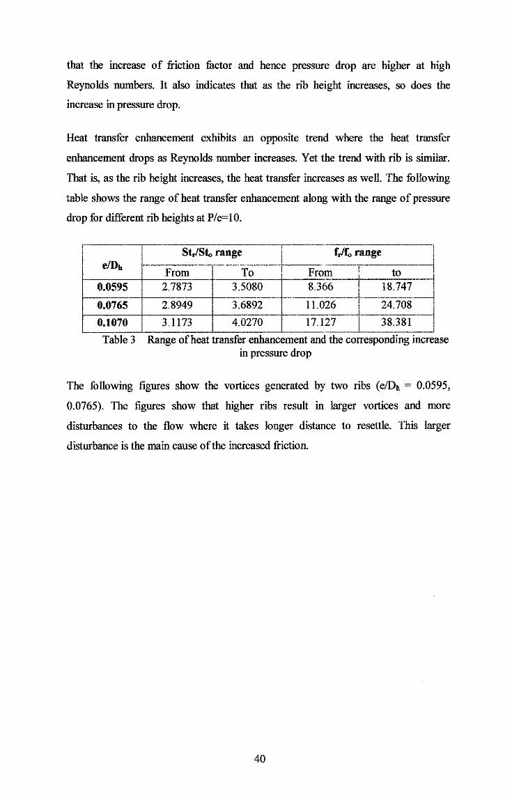
The following figures show the vortices generated by two ribs (e/Dh = 0.0595,

0.0765). The figures show that higher ribs result in larger vortices and more

disturbances to the flow where it takes longer distance to resettle. This larger

disturbance is the main cause of the increased friction.

40

Figure 38 Vortices generated by rib with e=0.0595

Figure 39 Vortices generated by rib with e=0.765

41

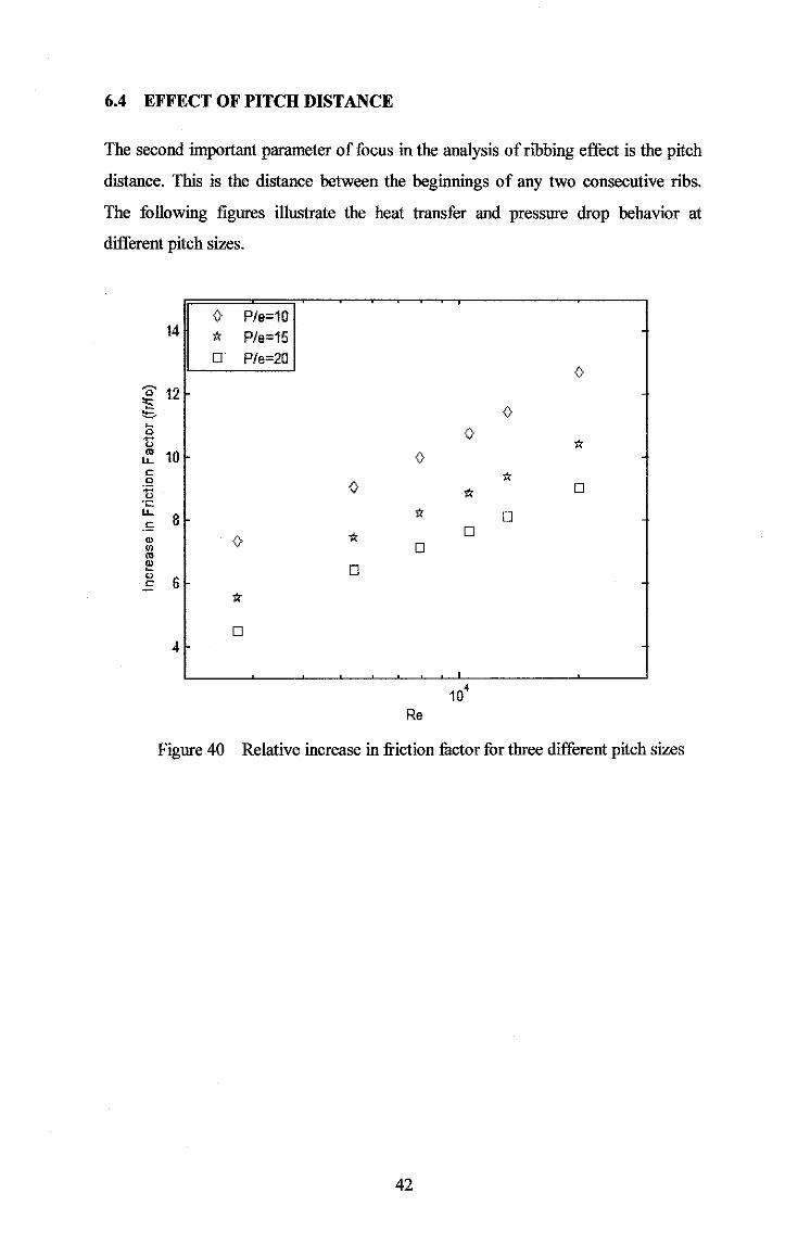
6.4 EFFECT OF PITCH DISTANCE

The second important parameter of focus in the analysis of ribbing effect is the pitch

distance. This is the distance between the beginnings of any two consecutive ribs.

The following figures illustrate the heat transfer and pressure drop behavior at

different pitch sizes.

Figure 40 Relative increase in friction fuctor for three different pitch sizes

42

4.5 {} Ple=10

"' Pie=15 D P/e=20

'0' 4 iii -., @. E {} ., 3_5 E {} ., 0 0 c {} "' 0 -"' "' "' 0 w - 3 "' "' .,

"' - D "' "' c D D D !'! D - D .. ..

2.5 I

Re

Figure 41 Heat transfer enhancement for three different pitch sizes

The observed trends from the previous figures show that increasing the pitch size

decreases both the relative increase of friction factor and heat transfer enhancement.

This is attributed to the fact that when the pitch distance increases, flow re-attachment

to the surfuce increases and vortices induced by the ribs tend to settle. While at small

pitches, re-attachment is less and vortices' wake is still active. This results in

increasing the pressure drop and enhancing the heat transfer. This result is in line

with the main objective of ribbing which is to induce vortices and turbulate the flow.

The following figures compare the velocity vectors at the vicinity of the ribs for two

different pitches (P/e = 10, P/e = 15). It is seen in the figures that flow settlement is

better at higher pitches where it is completely settled well before reaching the

following rib on the contrary to the case of smaller pitches.

43

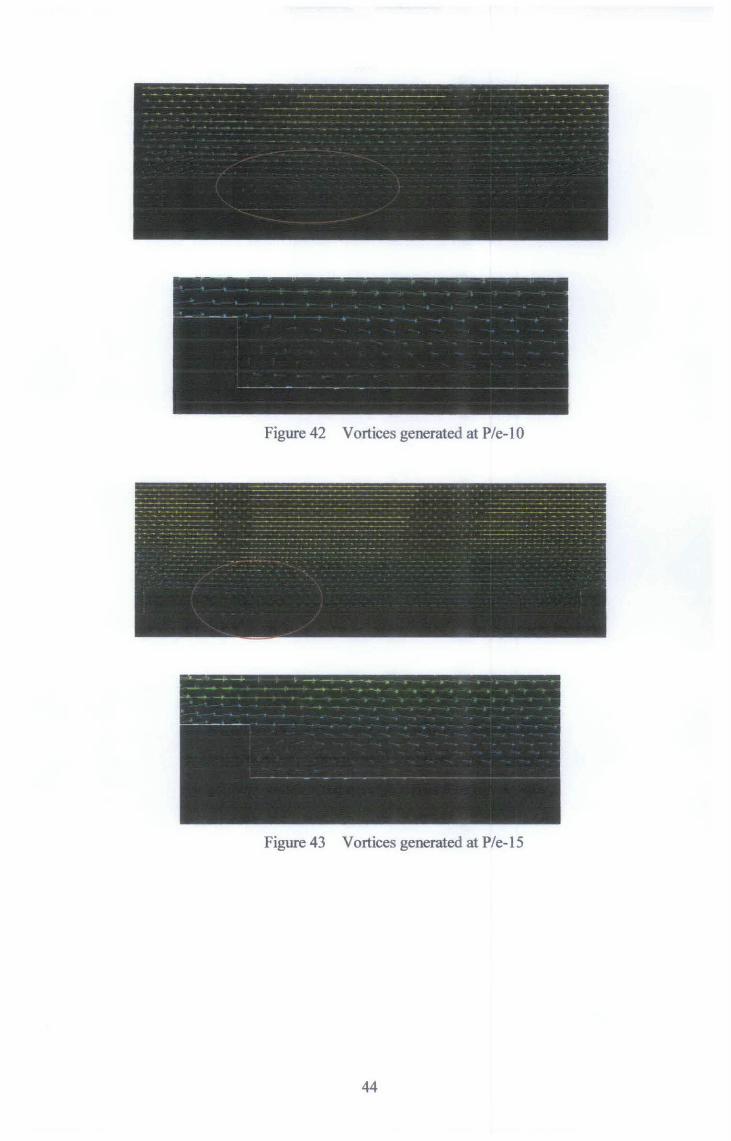
Figure 42 Vortices generated at P/e-10

Figure 43 Vortices generated at P/e-15

44

6.5 ANNULUS EFFICIENCY INDEX 11

The effect of both rib height and pitch distance was studied on the heat transfer and

pressure drop separately. Various trends were observed for each parameter resulting

from various aspects of the rib configuration (rib height and pitch). These various

trends pose the need of having a tool which allows studying the effect all ribbing

configurations on both heat transfer and pressure drop simultaneously. This tool, the

annulus efficiency index rJ, was introduced by Webb [2] and it is defmed as the

amount of pressure drop which must be sacrificed in order to achieve a given amount

of heat transfer enhancement. In mathematical form, it is the ratio of heat transfer

enhancement to the relative increase in friction factor:

!]= Str/Sto

frjfo (22)

The following figures show the efficiency index for different configurations. First,

the index is evaluated for cases l, 2, 3 both analytically and numerically and

compared with the corresponding experimental data (these figures show the index at a

single ribbing case). Later, the index is evaluated analytically for all ribbing

configurations which are combined in one figure.

45

P/e=15, eiDh = 0.0595 0.9

0 Experimentally

0.8 * Numerically D Analytically

07 X ., -a

"' 0.6 :>.

0 " c ., '" 05

0 E w ., D ::0 0.4 3 0 * "' D "' <:: 0 D -< "' 0.3 0 D

0 0 0

0.2

0.1 1()4

Re

Figure 45 Annulus efficiency index for ribbed case 2

46

0_9 0 Ple=10

0.8 * Ple=15 D Ple=20

0.7 X .. -u D <= 0_6 >-.

* u c -~ 0.5 u

0 ~ D w ., "' :::> 0.4 ::; 0 "' 0:: D 4:

0_3 * 0

0.2

0_1 ' ' 0.05 ()_06 0_07 0.08 0.09 0.1 0.11

e!Dh

Figure 47 Annulus Efficiency index (17) Vs rib height for different pitch sizes

47

The three comparison figures show that the analytical procedure gives excellent

estimate of the efficiency index for all cases. Numerical procedure too gives good

estimates of the index yet, discrepancies do occur for some cases. The discrepancy

source is due to the inherent error in estimating the friction factor as seen earlier.

A main observation regarding the efficiency index is that it assumes values less than

I all the time which indicates that the accompanying pressure drop outweighs the

heat transfer enhancement. Two more trends are observed in figure 42: first,

increasing the rib height results in decreasing the efficiency index. Second, as the

pitch distance increases, so does the efficiency index. The first trend implies that

increasing the rib height contributes more friction with decrease heat transfer

enhancement which explains the declining trend. The later implies that allowing the

flow to reattach to the surface before re-inducing the vortices yields better

enhancement in heat transfer than continuously inducing the vortices in the wake of

their predecessors this also explain the trends seen in section 5.4 where increasing the

pitch distance results in less pressure drop while it better enhances heat transfer.

Plotting a figure similar to figure 40 above on a wide range of pitches and rib heights

allows designers to optimize the ribbing configuration to match the available

pumping power with the desired heat transfer enhancement.

A final remark regarding the efficiency index is that it should not be miss interpreted.

That is, having low efficiency does not necessarily imply a low gain (heat transfer

enhancement). It may be due to losses (pressure drop) much greater than the gain

(e.g. efficiency of 0.5 may be a result of a ratio of 5/10 or 10/20. In the latter case,

more heat transfer enhancement is achieved which in some cases could be attractive

despite the 20 times pressure drop).

6.6 RIBS ON THE INNER PIPE

All the previous discussion was based on the case of ribs installed on the annulus. In

this section the effect of ribbing the inner pipe instead is discussed. The case of ribs

on the inner pipe was studied numerically and compared with a similar annulus

ribbing case (same e, P, and inlet parameters). The following figures compare the

48

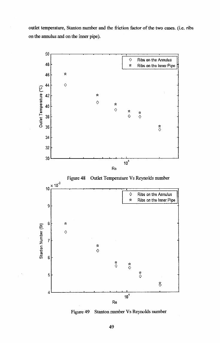
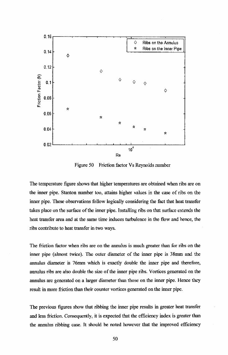
outlet temperature, Stanton number and the friction factor of the two cases. (i.e. ribs

on the annulus and on the inner pipe).

0 Ribs on the Annulus 48 tr Ribs on the Inner Pipe

46

34

32

Re

Figure 48 Outlet Temperature Vs Reynolds number

0 Ribs on the Annulus tr Ribs on the Inner Pipe

9

~

{§_ 8 tr

<; 0 ..c E

7 " z "' tr

" 0 1:! "' (j) 6

tr tr 0 0

5 tr 0

Re

Figure 49 Stanton number Vs Reynolds number

49

0.16 0 Ribs on the Annulus

"' Ribs on the Inner Pipe 0.14

0

0.12

0 "=· 5 0.1 0 0 -;:; "' 0 "--;:;: g 0.08 .2 .;:

0.06

0.04 "' "' 0.0.2

104

Re

Figure 50 Friction factor Vs Reynolds number

The temperature figure shows that higher temperatures are obtained when ribs are on

the inner pipe. Stanton number too, attains higher values in the case of ribs on the

inner pipe. These observations follow logically considering the fact that heat transfer

takes place on the surface of the inner pipe. Installing ribs on that surface extends the

heat transfer area and at the same time induces turbulence in the flow and hence, the

ribs contribute to heat transfer in two ways.

The friction factor when ribs are on the annulus is much greater than for ribs on the

inner pipe (almost twice). The outer diameter of the inner pipe is 38mm and the

annulus diameter is 76mm which is exactly double the inner pipe and therefore,

annulus ribs are also double the size of the inner pipe ribs. Vortices generated on the

annulus are generated on a larger diameter than those on the inner pipe. Hence they

result in more friction than their counter vortices generated on the inner pipe.

The previous figures show that ribbing the inner pipe results in greater heat transfer

and less friction. Consequently, it is expected that the efficiency index is greater than

the annulus ribbing case. It should be noted however that the improved efficiency

50

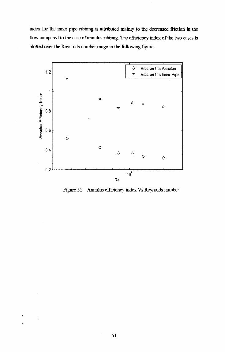
index for the inner pipe ribbing is attributed mainly to the decreased friction in the

flow compared to the case of annulus ribbing. The efficiency index of the two cases is

plotted over the Reynolds number range in the following figure.

0 Ribs on the Annulus 1_2 * Ribs on the Inner Pipe

1 " "' ., <:

'I< 'I< "' <> c 0_8 .!1! <> ~ w

"' :::! ;; 0_6 "' <: <l[ 0

0.4 0 0 0

0

0.2 ' 10

4

Re

Figure 51 Annulus efficiency index V s Reynolds number

51

Chapter 7

CONCLUSIONS AND RECOMMENDATIONS

7.1 CONCLUSIONS

The flow in a ribbed double pipe heat exchanger was modeled both analytically and

numerically on Reynolds number ranging from 2000 to 20,0000. The analytical

analysis is based on empirical equations and correlations introduced by previous

researchers in the field while the numerical analysis employed a commercially

available CFD code, FLUENT, to simulate the flow and evaluate its main properties

such as velocity, pressure and temperature.

Different ribbing configurations including various rib heights, pitch distances and

ribbing on the inner pipe were studied. The main parameters of focus are the heat

transfer enhancement expressed by Stanton number and the pressure drop expressed

by the friction factor.

The thermo fluid mechanisms governing the flow phenomena were studied based on

the obtained results to develop a generalized understanding of the heat transfer and

pressure drop behavior.

Ribbing was found to enhance the heat transfer by more than 3 times at an expense of

increasing pressure drop of more than 18 times. Ribbing on the inner pipe instead of

the outer pipe was found to yield better enhancement of heat transfer and less friction

losses.

52

7.2 RECOMMENDATIONS

Several other parameters need to be considered to come into full understanding of the

heat transfer and pressure drop with the presence of ribs, these parameters include:

1- To investigate the effect of the angle of attack on the performance of the heat

exchanger.

2- To investigate the effect of the shape angle on the performance of the heat

exchanger.

3- To investigate the phenomena on rectangular cross sections.

53

REFERENCES

[1] Nikuradse, J., "Laws for Flow in Rough Pipes", VDI Forsch.361, series B, 4

NACA YM, 1950

[2] Webb, R L., Eckert, E. R G. And Goldstein, R J., "Heat Trausfer and Friction in

Tubes with Repeated-Rib Roughness", Int. J. Heat Mass Transfer, Vol 14, pp. 601-

617, 1970

[3,a] Kazuyuki Takase, "Experimental Results of Heat Trausfer Coefficients and

Friction Factors in a 2D /3D Rib-Roughened Annulus",

[3,b] Kazuyuki Takase, "Nwnerical Prediction of Augmented Turbulent Heat

Trausfer in an Annular fuel Channel with Repeated Two-Dimensional Square Ribs",

Nuclear Engineering and Design 165 (1996) 225 237

[4] Cengiz Yildiz, Yasar Bicer and Dursun Pehlivan, "Effect of Twisted Strips on

Heat Transfer and Pressure Drop in Heat Exchangers", Energy Convers, Mgmt Vol.

39, No. 3/4, pp. 331-336, 1998.

[5] H. Braun, H. Newnann, N.K. Mitra, "Experimental and Numerical Investigation

of Turbulent Heat Trausfer in A Channel with Periodically Arranged Rib Roughness

Elements", Experimental Thermal and Fluid Science 19 (1999) 67±76.

[6] Laheeb, A.-H. N. (1999). Performance Enhancement of Double Pipe Heat

Exchangers by Enforced Turbulence on Single Surface. Baghdad.

[7] Hac1 Mehmet Sahin, Ali Riza Da~ EsrefBays~ "3-D Numerical Study On The

Correlation Between Variable Inclined Fin Angles And Thermal Behavior In Plate

Fin-Tube Heat Exchanger", Applied Thermal Engineering 27 (2007) 1806-1816.

[8] Al-Kayiem,H.H, Al-Habeeb,L.N, "Performance Enhancement of Double Pipe

Heat Exchangers by Enforced Turbulence on Single Surface", International

Conference Plant Equipment and Reliability, The Equipment Chapter. 27-28, March.

Sunway Lagoon, Malaysia 2008.

[9] Veysel Ozceyhan, Sibel Gunes, Orhan Buyukalaca, Necdet Altuntop, "Heat

Trausfer Enhancement in Tubes Using Circular Cross Sectional Rings Separated from

the Wall", Journal of Applied Energy 85 (2008) 988-1001

54

[10] Kakac, Paykoc, "Basic Relationships for Heat Exchangers", NATO Scientific

Affairs Division, Vol143, pp.29-80, (1988)

[11] Han, J. C., Glicksman, L. R. And Rohsenow, W. M., "An Investigation of Heat

Transfer and Friction Factor for Rib-Roughened Surfaces", Int. J. Heat Mass

Transfer, Vol. 21, pp.l143-1156,1978.

[12] Webb, R. L., Eckert, E. R. G. And Goldstein, R. J., "Heat Transfer and Friction

in Tubes with Repeated-Rib Roughness", Int. J. Heat Mass Transfer, Vol. 14, pp.

601-617, 1971.

[13] H.K.Versteeg, & Malalasekera, W. (1995). An introduction to computational

fluid dynamics, the finite volume method. Prentice Hall.

55

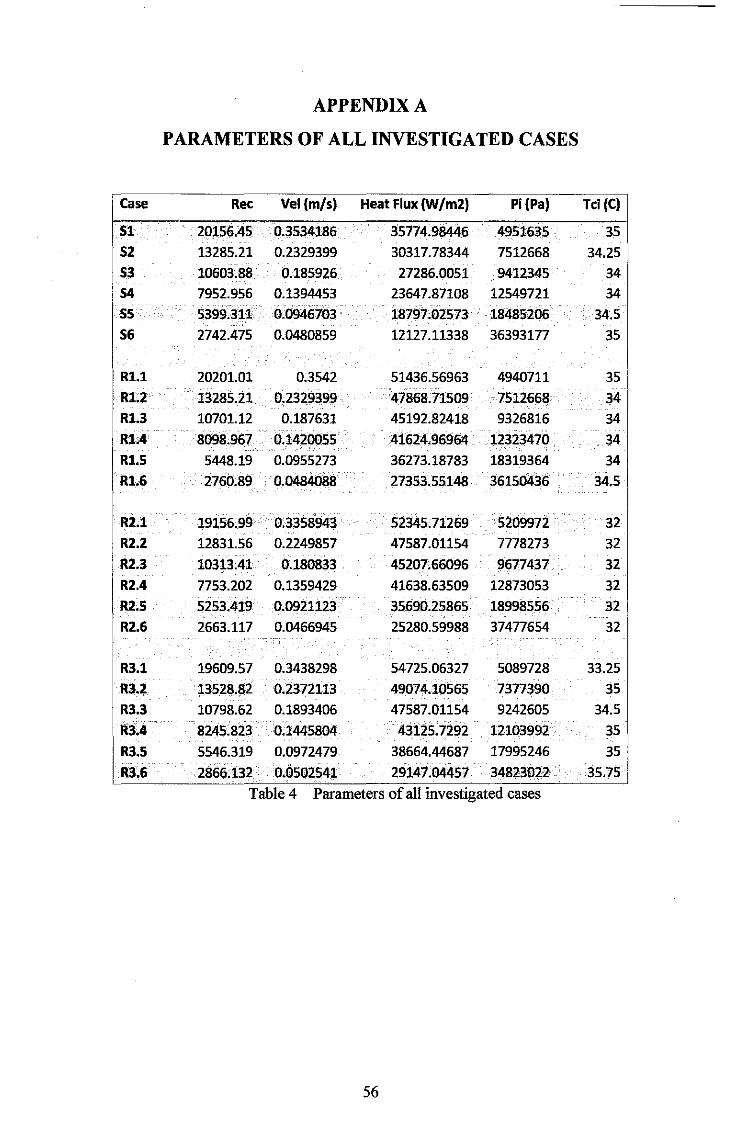
APPENDIX A

PARAMETERS OF ALL INVESTIGATED CASES

Case Rec Vel {m/s) Heat Flux {W/m2) Pi {Pa) Tci {C)

51 20156.45 0.3534186 35774.98446 4951635 35 52 13285.21 0.2329399 30317.78344 7512668 34.25

53 10603.88 0.185926 27286.0051 9412345 34 54 7952.956 0.1394453 23647.87108 12549721 34 55 5399.311 0;0946703 18797;02573 18485206 . 34.5

56 2742.475 0.0480859 12127.11338 36393177 35

R1.1 20201.01 0.3542 51436.56963 4940711 35

R1.2 13285.21 0.2329399 47868.71509 . 7512668 34 R1.3 10701.12 0.187631 45192.82418 9326816 34

R1.4 8098.967 0.1420055 41624.96964 12323470 34

Rl.S 5448.19 0.0955273 36273.18783 18319364 34

IU.6 2760.89 0.0484088 27353.55148 36150436 34.5

R2.1 19156.99 0:3358943 52345.71269 . 5209972 32 R2.2 12831.56 0.2249857 47587.01154 7778273 32

R2.3 10313.41 0.180833 45207.66096 9677437 32

R2.4 7753.202 0.1359429 41638.63509 12873053 32

R2.5 5253.419 0.0921123 35690.25865 18998556 32

R2.6 2663.117 0.0466945 25280.59988 37477654 32

R3.1 19609.57 0.3438298 54725.06327 5089728 33.25

R3.2 13528.82 0.2372113 49074.10565 7377390 35

R3.3 10798.62 0.1893406 47587.01154 9242605 34.5

R3.4 8245:823 0.1445804 43125.7292 12103992 35

R3.5 5546.319 0.0972479 38664.44687 17995246 35

R3.6 2866.132 . 0.0502541 29147.04457 34823022 35.75 I

Table 4 Parameters of all investigated cases

56

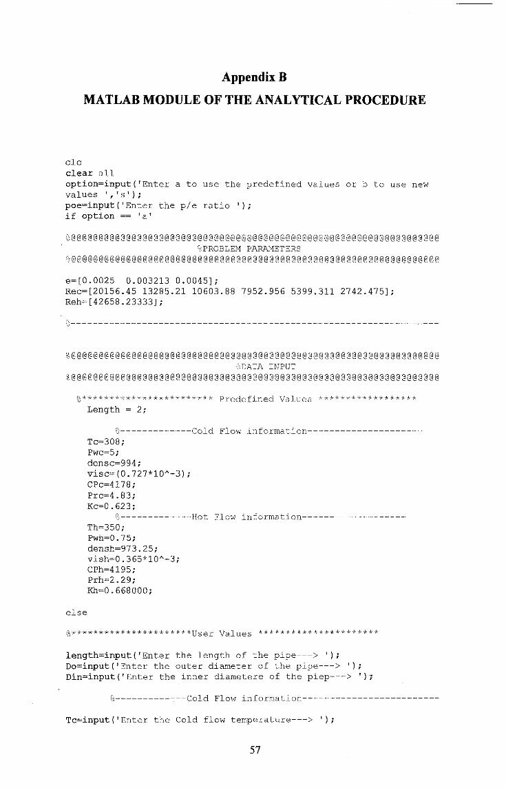
Appendix B

MATLAB MODULE OF THE ANALYTICAL PROCEDURE

clc clear all option=input('Enter a to use the predefined values orb to use new values ' , 's' ) ; poe=input('Enter the p/e ratio '); if option== 'a'

%@@@@@@@@@@@@@@@@@@@@@@@@@@@@@@@@@@@@@@@@@@@@@@@@@@@@@@@@@@@@@@@@@@@ %PROBLEM PARAMETERS

%@@@@@@@@@@@@@@@@@@@@@@@@@@@@@@@@@@@@@@@@@@@@@@@@@@@@@@@@@@@@@@@@@@@

e=[0.0025 0.003213 0.0045]; Rec=[20156.45 13285.21 10603.88 7952.956 5399.311 2742.475]; Reh=[42658.23333];

0-------------------------------------------------------------------

%@@@@@@@@@@@@@@@@@@@@@@@@@@@@@@@@@@@@@@@@@@@@@@@@@@@@@@@@@@@@@@@@@@@ ':DATA INPUT

%@@@@@@@@@@@@@@@@@@@@@@@@@@@@@@@@@@@@@@@@@@@@@@@@@@@@@@@@@@@@@@@@@@@

9s ** * * * * ** * * * * * * * ** * ** * ** * Predefined Values * * ** * ** * * * * * * * * * ""'* Length = 2;

else

'3;---------------Cold Flow information--·------------------­

Tc=308; Pwc=5; densc=994; visc=(0.727*10A-3); CPc=4178; Prc=4.83; Kc=0.623;

%-------------Hot Flow information------------------­Th=350; Pwh=0.75; densh=973.25; vish=0.365*10A-3; CPh=4195; Prh=2.29; Kh=0.668000;

-~, * ** * * * * * * * * * * *********User Values * * * ** * * * * * ** * * * * * * * * * *

length=input('Enter the length of the pipe---> '); Do=input('Enter the outer diameter of the pipe---> '}; Din=input('Enter the inner diametere of the piep~~-> ');

1_,- ------------Cold Flow info rma ti on--·-----------------------

Tc=input{'Enter the Cold flow temperature---> ');

57

Pwc=input('Enter the Cold pump power---> '); densc=input('Enter the cold flow density---?'); velc=input('Enter cold flow velocity--->'); visc=input('Enter the cold flow viscosity--->'); CPc=input('Enter the cold flow Cp--->'); Prc=input('Enter the cold flow Pr---> '); Kc=input('Enter the cold flow thermal condcutivity ---->');

%-------------Hot Flow information-------------------------

Th=input('Enter the Hot flow temperature---> '); Pwh=input('Enter the hot pump power---> '); densh=input('Enter the hot flow density---?'); vish=input('Enter the hot flow viscosity--->'); CPh=input('Enter the hot flow Cp--->'); Prh=input('Enter the hot flow Pr---> '); Kh=input('Enter the hot flow thermal condcutivity ---->'); end

%@@@@@@@@@@@@@@@@@@@@@@@@@@@@@@@@@@@@@@@@@@@@@@@@@@@@@@@@@@@@@@@@@@@ 'j SMOOTH CASE

%@@@@@@@@@@@@@@@@@@@@@@@@@@@@@@@@@@@@@@@@@@@@@@@@@@@@@@@@@@@@@@@@@@@

Dh=0.042; Dhh=0.0254; Rh=20000; Rc=20000; for j=l:length(Reh)

%-------------Friction Factor------------------------for i=l:length(Rec)

frbc(i)= (0.079l)*((Rec(i))A(-0.25)); frmcc(i)=0.0014+0.125*Rec(i)A(-0.32); frbh(j)= (0.079l)*(Reh(j))A(-0.25); frmch(j)=0.0014+0.125*Reh(j)A(-0.32); fra=(frbc+frmcc)/2;

!,j-------------Nus sul t Number---------------------------­

Nuc(i)= 0.023*((Rec(i))A0.8)*(Prc)A0.4; ?, cold side Nuh(j)= 0.023*((Reh(j))A0.8)*(Prh)A0.3; '0 Hot Side

S-------------Heat Transfer Coefficient----------------hc(i)=(Nuc(i)*Kc)/Dh; ~ cold side hh (j) = (Nuh (j) *Kh) /Dhh; 2 Hole Side

~o-------------Stanton Number---------- -----------------

Stc(i)= Nuc(i)/(Rec(i)*Prc); Sth(j)= Nuh(j)/(Reh(j)*Prh);

end end

~. cold side _,, Hot Side

%@@@@@@@@@@@@@@@@@@@@@@@@@@@@@@@@@@@@@@@@@@@@@@@@@@@@@@@@@@@@@@@@@@@ %RRIBBED CASE

%@@@@@@@@@@@@@@@@@@@@@@@@@@@@@@@@@@@@@@@@@@@@@@@@@@@@@@@@@@@@@@@@@@@

frrc=zeros(size(e));

58

for j~1:length(e) for i~1:length(Rec)

ep~1;

lirnit=1; while limit> 0.001

if ep<35 rn=-0.4;

else m=O;

end

if poe<10 n=-0.13;

else n=0.35;

end

frrc(i,j) = 2/(((3.300722/(10/poe)An) * (ep/35)A(rn)- 2.5 * log(2*e(j)/Dh) - 3.75)A2);

epc= (e(j)/Dh)* Rec(i)* (frrc(i,j)/2)A0.5;

lirnit~abs((epc- ep)/ep); ep=epc;

end eplus(i)=ep;

if eplus(i)<35 rn=-0.4;

else rn=O;

end

if eplus(i)<35 d~ 1;

else d= 0.28;

end

if poe<10 n=-0.13;

else n=0.35;

end Replus(i)= (3.300722/((poe/10)An))*(eplus(i)/35)Arn;

% (Roughness Function) Hew(i,j)~4.5*((eplus(i))A0.28)*(PrcA(0.57));

Correlation) Heh(i,j)~(8*(eplus(i)/35)A(d))/(2)A(-0.45);

Correlation)

~' (vleb

(Han

stw(i,j)= frrc(i,j)/(((Hew(i,j)­Replus(i))*((2*frrc(i,j))A(Q.5)))+2); SStanton Number w.ith vleb correlation

sth(i,j)= frrc(i,j)/(((Heh(i,j)­Replus(i))*((2*frrc(i,j))A(0.5)))+2); SStanton Number with Han correlation

sta~(stw+sth)/2;

end end

59

for j=l:length(e)

end

for i=l:length(Rec)

end

enhst (:, j) =stw (:, j) . /Stc'; enhfr(:,j)=frrc(:,j) ./fra';

60

AppendixC

MATLAB MODULE OF THE NUMERICAL PROCEDURE

'2:* * ** * ** * * * * ** * * * * * GEOMETRY INFORMATION*****·.~-*********** Dh=0.042; Dhh=0.0254; Do=0.0342; Ah=pi*2*Do; Ks=30.7;

~-------------Cold Flow information--------------------­Pwc=S; densc=994; visc=(0.732*1QA-3); CPc=4178; Prc=4.91; Kc=0.624;

~-------------Hot Flow information-------------------­Pwh=0.75; densh=973.25; vish=0.365*1QA-3; CPh=4195; Prh=2.29; Kh=0.668000;

%****************** h FOR HOT FLOW***********+****************** velhot=vish*Reh/(densh*Dhh); mh=densh*velhot*pi*(DhhA2)/4; hh=Q.023*RehA(Q.8)*PrhA(Q.3)*Kh/Dhh;

for i=l:length(Tci) delth(i)=Thi(i)-Tho{i); deltc{i)=Tco{i)-Tci{i); velcold(i)=visc*Rec(i)/{densc*Dh); mc(i)=densc*velcold{i)*pi*(DhA2)/4; delta(i)= Tho{i)-Tci{i); deltb{i)= Thi(i)-Tco(i); LMTD{i) = (deltb(i)-delta{i))/log(deltb{i)/delta(i));

------- LNTD------------------

Q(i)=mh*CPh*delth{i);

uo{i)= Q{i)/(Ah*LMTD{i));

a=(Do/{Dhh*hh))+O.S*Do*{log{Do/Dhh))/Ks; ho{i)={uo{i)A(-1)-a)A{-1);

Nuc(i)= ho{i)*Dh/Kc; Stc{i)= Nuc(i)/(Rec(i)*Prc);

delp(i)= abs(pe(i)-po(i)); f(i)=delp(i)/((8*500*(vel(i))A2)/0.042); end

61

Case To (exp) To (num) Pi Po

R 1.1 36.75 37.11 25.220 -630.911

R1.2 36.25 37.00 10.869 -296.785

R 1.3 37 37.53 7.214 -223.222

R 1.4 38 38.40 4.117 -129.092

R 1.5 39 39.67 1.841 -64.525

R 1.6 40 42.97 0.470 -18.816

R2.1 34 34.3016 21.4774 -667.977

R2.2 34.5 35.0807 9.216306 -320.674

R2.3 35 35.6688 5.840482 -220.722

R2.4 35.25 36.4126 3.501422 -131.955

R2.5 37 37.7147 1.729912 -48.0847

R2.6 38.5 39.7213 0.4288 -12.7309

APPENDIXD

SIMULATION RESULTS

Vm Delta P St (exp)

0.3057 656.131 0.0036

0.2010 307.654 0.0041

0.1630 230.436 0.0044

0.1234 133.209 0.0048

0.0830 66.366 0.0055

0.0421 19.286 0.0067

689.455 0.335894 0.00315

329.890 0.224986 0.00353

226.562 0.181 0.00388

135.457 0.135943 0.00428

49.815 0.092112 0.00478

13.160 0.046694 0.00544

62

St (num) St(Webb) fr (exp) fr(num) fr(Webb)

0.0037 0.0039 0.0842 0.0737 0.0843

0.0042 0.0043 0.0855 0.0800 0.0843

0.0044 0.0046 0.0857 0.0911 0.0843

0.0047 0.0050 0.0852 0.0919 0.0843

0.0052 0.0055 0.0854 0.1012 0.0843

0.0065 0.0065 0.0836 0.1143 0.0816

0.0033 0.0035 0.0655 0.0642 0.0692

0.0037 0.0039 0.0668 0.0684 0.0692

0.004 0.0042 0.0666 0.0726 0.0692

0.0044 0.0045 0.0667 0.0578 0.0692

0.0047 0.005 0.0657 0.0616 0.0692

0.0052 0.0057 0.0646 0.0634 0.0618

51.1 36.5 36.4365 -0.30152 -93.997 93.69551 0.353419 0.0013 0.0012 0.0012 0.0068 0.0079 0.0066

51.2 36 36.4225 -0.15257 -46.3716 46.21906 0.23294 0.0014 0.0013 0.0013 0.0075 0.0089 0.0074

51.3 36 37.4685 -0.10749 -31.5665 31.45902 0.185926 0.0015 0.0014 0.0014 0.0078 0.0096 0.0078

51.4 36 36.7603 -0.06949 -19.5253 19.45579 0.139445 0.0016 0.0015 0.0015 0.0085 0.0105 0.0084

51.5 37.5 37.3465 -0.04044 -10.5101 10.46962 0.09467 0.0018 0.0016 0.0016 0.0095 0.0123 0.0093

51.6 38.57 38.6278 -0,0172 -3.93898 3.921782 0.048086 0.0020 0.0019 0.0018 0.0115 0.0178 0.0111

R3.1 35.75 35.5554 -2.16123 -1016.43 1014.265 0.34383 0.00412 0.0044 0.0044 0.179 0.0901 0.1728 ----------------

R3.2 37.25 37.9896 -1.05499 -533.037 531.9822 0.237211 0.00484 0.0049 0.0049 0.180 0.0993 0.1728

R3.3 37.5 38.1259 -0.68651 -346.324 345.6374 0.189341 0.00537 0.0054 0.0052 0.184 0.1012 0.1728 -- - - --- - -

R3.4 39 39.3011 -0.43074 -207.399 206.9678 0.14458 0.00581 0.0055 0.0057 0.180 0.104 0.1728

R3.5 40 40.7065 -0.20621 -103.765 103.5589 0.097248 0.00674 0.0064 0.0063 0.179 0.115 0.1728

R3.6 43 44.0559 -0.06357 -32.5634 32.4998 0.050254 0.00825 0.0075 0.0076 0.181 0.1351 0.1728

Table 5 Simulation results

63

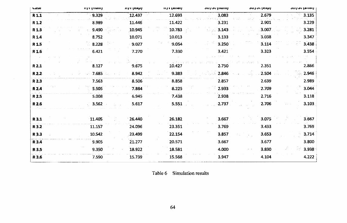
to..d:Jt: If /I \IIUIIIJ II/I \CAtiJ llfl \CIIICIII on.rt~L \111.11111 ~t.lf~L \'IC'At'J O;U.I/•;n. \CIIICIIJ

R1.1 9.329 12.437 12.693 3.083 2.679 3.135

R1.2 8.989 11.446 11.422 3.231 2.901 3.229

R 1.3 9.490 10.945 10.783 3.143 3.007 3.281

R 1.4 8.752 10.071 10.013 3.133 3.038 3.347

R 1.5 8.228 9.027 9.054 3.250 3.114 3.438

R1.6 6.421 7.270 7.330 3.421 3.323 3.554

R2.1 8.127 9.675 10.427 2.750 2.351 2.866

R2.2 7.685 8.942 9.383 2.846 2.504 2.946 - - ------- ~-

R2.3 7.563 8.506 8.858 2.857 2.639 2.989

R2.4 5.505 7.884 8.225 2.933 2.709 3.044

R 2.5 5.008 6.945 7.438 2.938 2.716 3.118 I

I R2.6 ~ 3.562 5.617 5.551 2.737 2.706 3.103

I R3.1 11.405 26.440 26.182 3.667 3.075 3.667

R3.2 11.157 24.096 23.351 3.769 3.433 3.769

R3.3 10.542 23.499 22.154 3.857 3.653 3.714

R3.4 9.905 21.277 20.571 3.667 3.677 3.800

R3.5 9.350 18.922 18.581 4.000 3.830 3.938

R3.6 7.590 15.739 15.568 3.947 4.104 4.222

Table 6 Simulation results

64