N A S A TECHNICAL NOTE

THEORY OF THE ANISOTROPIC HEISENBERG FERROMAGNET

by Lawrence Flax

Lewis Research Center Cleveland, Ohio 44135

N A T I O N A L AERONAUTICS A N D SPACE A D M I N I S T R A T I O N W A S H I N G T O N , D. C. OCTOBER 1970

https://ntrs.nasa.gov/search.jsp?R=19700033052 2020-03-27T01:09:48+00:00Z

TECH LIBRARY UAFB, NM

9. Performing Organization Name and Address

Lewis Resea rch Center National Aeronautics and Space Administration Cleveland, Ohio 44135

National Aeronautics and Space Administration 12. Sponsoring Agency Name and Address

l Washington, D.C. 20546

i 15. Supplementary Notes

I Illill lllll1 lllll llllllll111111llllll Ill

17. Key Words (Suggested by Authods) I Heisenberg ferromagnet ism Anisotropic Phase t ransi t ions Green 's function Watson's s u m s Decoupling approximations

2. Government Accession No. I 1. Report No. I NASA TN D-6037 - .

4. Title and Subtitle

THEORY O F THE ANISOTROPIC HEISENBERG FERROMAGNET

18. Distribution Statement Unclassified - unlimited

7. Author(s1

Lawrence Flax

19. Security Classif. (of this report) 20. Security Classif. (of this page) 21. NO. of Pages

Unclassified Unclassified 53 22. Price"

$3.00

- OL32b78 3. Recipient's Catalog No.

5. Report Date October 1970

6. Performing Organization Code

8. Performing Organization Report No.

E-5715 10. Work Unit No.

129-02 11. Contract or Grant No.

13. Type of Report and Period Covered

Technical Note 14. Sponsoring Agency Code

~~

16. Abstract

The development of a fo rma l i sm for the investigation of phase t ransi t ions of the anisotropic Heisenberg ferromagnet is presented. is determined by s e v e r a l decoupling schemes . A method of calculating the generalized Watson sums is a l s o formulated.

By the u s e of Green's function theory, the magnetization

The thermodynamic quantity to be studied is the magnetization at and

THEORY OF THE ANISOTROPIC HEISENBERG FERROMAGNET

by Lawrence Flax

Lewis Research Center

SUMMARY

The development of a formalism f o r the investigation of phase transit ions of the anisotropic Heisenberg ferromagnet is presented. the magnetization is determined by seve ra l decoupling schemes. the generalized Watson sums is also formulated.

point. An analytical formulation is developed to determine at what temperature the transition takes place.

By the use of Green's function theory A method of calculating

The thermodynamic quantity to be studied is the magnetization a t and near the Curie By use of various decoupling schemes, different phase transit ions a r e generated.

INTRODUCTION

As the temperature of a ferromagnet is increased, the magnetization will decrease until, a t a temperature known as the Curie temperature Tc the sample becomes para- magnetic. re fe r red to as the ferromagnetic phase transition. theory of ferromagnetism is the theoretical description of the phase transition. theory of this phase transition, as well as many other types of phase transitions occur- ring in nature, has been the subject of many investigations. These investigations have shown that electrical , mechanical, and many thermodynamic properties of a mater ia l a r e a l tered when the mater ia l undergoes a phase transition.

One way of describing the ferromagnetic phase transition is to look upon i t as an order-disorder transition in the material . the correlation between the propert ies of two atoms, even when the atoms are widely separated in space. The spontaneous magnetization present in a ferromagnet is due to the correlations between the spins of the atoms. Above the Curie temperature the long- range o rde r is gone, and the system is paramagnetic. f rom an ordered to a disordered s ta te is the description of the thermodynamic phase transition.

The process by which this change f r o m ferromagnet to paramagnet occurs is The fundamental problem in the

The

The property of o rde r in a system describes

The description of this change

Thermodynamic phase transit ions can be classified by the discontinuities that occur in the Gibbs thermodynamic potential. F r o m an experimental standpoint, it is not easy to decide what types of transit ion are present because of the rapid variation of a thermo- dynamic variable such as specific heat or entropy, near the cr i t ical temperature. It is often difficult to distinguish, fo r example, whether a transit ion in specific heat against temperature has a finite, infinite, o r cusp discontinuity.

This report is concerned with the investigation of the thermodynamic properties of the anisotropic Heisenberg ferromagnet. The thermodynamic quantity studied was the magnetization at and near the Curie point. thermodynamics of the system was the double t ime thermodynamic Green's functions. The objectives of this report are threefold: One is to investigate the various decoupling schemes f o r the Green's function theory of the anisotropic Heisenberg model. The sec- ond purpose is the evaluation of the generalized Watson sums, which a r i s e in the theory of magnetism and other order-disorder phenomena, in analytical form. These sums must be evaluated in o rde r to calculate the thermodynamic quantities of interest as a function of temperature. Previous calculations of the generalized Watson sums have been mostly based on series expansions and a r e therefore valid only over limited tem- perature regions. sums without using s e r i e s expansions o r extensive computer summations. objective is to propose a new type of decoupling. cally possible to have different orders of transit ions fo r the anisotropic Heisenberg model.

-

The s ta t is t ical method used to determine the

The purpose here is to descr ibe a method of evaluating the Watson The third

This report shows that it is theoreti-

The simplest way of treating correlations between atoms in a ferromagnetic c rys ta l is to consider only one atom and replace i ts interaction with the rest of the c rys ta l by an effective field. Weiss (ref. l) , who assumed the effective field to be proportional to the magnetization. This theory gave a satisfactory qualitative picture of the main features of a ferromagnet, namely, the existence of a transition temperature, specific heat anomaly, and a sponta- neous magnetization. It had weak points, however, such as its fai lure to predict the cor rec t behavior of these quantities a t very low temperatures and i t s underestimation of the transition temperature. It a lso failed to explain the origin of the molecular field.

Not until the advent of quantum mechanics could the Weiss molecular field be justi- fied. Heisenberg (ref. 2 ) showed that this field is a resul t of a quantum-mechanical ex- change interaction. The exchange interaction is a consequence of the Pauli principle that requires the wave function to be antisymmetric with an exchange of space and spin coor- dinates. tends to orient the spin angular momenta and hence affect the magnetic moments of the atoms.

This theory, called the molecular field theory, was f i r s t advanced by

T h s exchange interaction can be interpreted naively as an interaction which

Dirac (ref . 3 ) formulated a Hamiltonian which displays the effect of coupling of spin

2

angular momenta of localized par t ic les . This Hamiltonian Heisenberg model, the mathematical statement of which is

is often re fer red to as the

(1)

where J., is the exchange interaction between the spins on sites i and j and the summation is over all sites. The vector spin of the ith particle is Si.

as a phenomenological constant, which is determined by fitting the theory with a set of experimental results.

In principle, all the thermodynamic and magnetic propert ies of a crys ta l that con- tains N lattice points can be determined by constructing the partition function fo r the Hamiltonian, and taking the appropriate derivatives. In practice, i t has not been pos- sible to solve this problem only for certain limiting cases . The only solutions that have been obtained for the Heisenberg model are fo r very high or very low temperatures. These solutions have been derived f rom s e r i e s expansions of the free energy in powers of T (the spin wave solution) valid fo r T << Tc and in powers of 1/T fo r T >> Tc. Each of these solutions is only valid far f rom the transition temperature and therefore various approximations have been proposed to study the behavior a t intermediate tem- peratures .

The existence of a phase transit ion in a system with long-range coupling is a ques- tion for s ta t is t ical mechanics. At the present this question cannot be answered mathe- matically fo r the full exchange interaction. solutions will provide both physical guides of the choice of approximation to be applied and the c r i te r ia against which to judge these approximations.

Perhaps the most powerful technique in the study of ferromagnetism is the method of temperature-dependent Green's functions (refs . 4 and 5). With this method the thermodynamics as well as the correlations of the spins can b e analyzed. Green's func- tion theory when applied to ferromagnetism agrees with the spin wave theory at low tem- peratures and with the 1/T expansion at high temperatures.

avoided if the Ising (ref. 6 ) model is used ra ther than the Heisenberg model. Heisenberg model, one assumes that the instantaneous values of the neighboring spins may be replaced by their t ime averages, then one obtains an Ising model. The Ising model may, however, be considered the Limiting case of the Heisenberg model, in which the exchange forces are extremely anisotropic in the z direction, and thus the Hamil- tonian is just

1J

The exchange interaction is positive fo r ferromagnetism and in practice is regarded

But the known (high and low temperature)

Some of the complications of the quantum mechanical theory of ferromagnetism are If, in the

3

i j

The suppression of the x and y components of the spin in this model produces consequences that must be t reated with caution. This model is incorrect at low temper- a tures because it excludes spin waves. elementary excitations occurs because the quadratic x and y dependence of the energy is neglected. The advantages of the Ising model is that calculations can often be carr ied out with r igor and it can be solved exactly in one and two (ref. 7 ) dimensions.

tization proving that the system is ferromagnetic. Heisenberg model has no ferromagnetism. In three dimensions, by the use of various approximations (refs. 8 to lo) , the thermodynamics of these models can be estimated. The resul ts of these approximations show that both models appear to exhibit a fe r ro- magnetic behavior.

dimensions, there. are other apparent differences in three dimensions. quantities like magnetization and susceptibility behave differently below the transition temperature. magnetic state.

considered an intermediate model. They have studied the cr i t ical behavior of this aniso- tropic model i n two and three dimensions for intermediate values of an anisotropy param- eter q, where 0 i q _r 1, by the Green function method and series expansion technique. The Ising and isotropic Heisenberg models are special cases with values of q equal to 0 and 1, respectively. The Dalton and Wood Hamiltonian is

The absence of spin waves o r low-temperature

The exact solution of the two-dimensional Ising model shows a spontaneous magne- In contrast , the two-dimensional

Besides the contrasting behavior pattern of the Ising and Heisenberg models in two Thermodynamic

The only place where both models show s imi l a r behavior is in the para-

Because of the diss imilar behavior of these models, Dalton and Wood (ref. 11) have

i j

where

( 3 )

In a physical sense , r ] can be interpreted as a strength parameter fo r an anisotropic exchange interaction. It is usually so interpreted f o r the case of ferromagnetic crystals where crystal field effects give r i s e to magnetic anisotropy. can have significant effects on the correlation and long-range o rde r properties of the system.

The magnetic anisotropy

4

The exact equations of motion fo r any o rde r of the Green's functions for the aniso- tropic Heisenberg model involve higher order Green's functions. Green's functions thus necessitate a decoupling approximation in o rde r to obtain a solv- able closed system of equation. the thermodynamics of the sys tem can be exposed. Various types of phase transit ions are predicted, depending on the fo rm of the decoupling parameter . This will involve a solution for the magnetization that will be valid for all temperature regions of interest without the use of any separa te approximations for high or low temperature regions.

These higher o rde r

F r o m these equations the correlation function and hence

REVIEW OF MOLECULAR FIELD THEORY OF FERROMAGNETISM

A qualitative understanding of the Weiss molecular field theory can be obtained by examining the k i n g Hamiltonian of equation (2). the statement that a spin S: feels an effective field

This equation may be considered to be

where the sum is over all nearest neighbor s i tes of the s i t e i, such that the Hamiltonian is

H = - E X i $ i

It is assumed here that the exchange energy between nearest neighbor electrons of the same atom is constant and that all electrons have the s a m e exchange energy. Only nearest neighbor interactions are included. of replacing equation (5) by

The molecular field approximation consists

(Xi) = Jz(S7)

where z is the number of nearest neighbors. The process of replacing the spin oper- a tor Sz by its s ta t is t ical average (S?) is the essential approximation of this method. The replacement is equivalent to neglecting fluctuations of (Sy) , if Sf is up, its neigh- bors will have more than average predilection for being up. The problem is then reduced essentially to treating a paramagnetic gas of noninteracting spins.

magnetic moment of the c rys ta l by

.l J

As all the magnetic a toms are identical and equivalent, (SF) is related to the total

5

M = N(SZ) J (7)

where N is the number of a toms and M is the magnetization. Equation (5) can then be writ ten in the form

ZJ N

(Xi) = - M

The thermodynamic quantities can b e determined directly f rom the partition func- tion. It is a straightforward matter to calculate the average z component of spin

where

Writing out the t r a c e for spin 1/2 a

r /

g=- 1 KT

d sett ing (SB) = (sz) yi

o r

2

Ids

(9)

using (Xi) = J( Sz) . Comparison with various experimental data gives a surprisingly good qualitative picture of the thermodynamic properties such as the temperature depen- dence of the magnetization, susceptibility, and specific heat. However, the molecular field theory does not descr ibe accurately the exact behavior of a spin system near abso- lute zero o r the Curie point.

There have been many extensions of and improvements to the Weiss theory for both ferromagnets and antiferromagnets. In the molecular-field theory approach, the ex- change interactions in the crystal are replaced by an effective field, so that certain

6

- - interactions ar is ing f rom S * S are lost. If the exchange interaction were to be consid- ered, the problem would become unmanageable. A compromise has been sought where a sma l l section of the c rys ta l is treated; the exchange interaction in this region can be solved exactly. The effect of the remainder of the c rys ta l was then taken to be an effec- tive field. The first detailed t reatment of the exchange-coupled spin pair in an effective field was given by Oguchi (ref. 12). He considered the effective field to be a molecular field which is proportional to the average magnetization. This method was an improve- ment over the Weiss field theory in describing short-range o rde r above the cr i t ical point, and i t gave a nonvanishing specific heat. On the other hand, it failed for the tem- perature dependence of magnetization near absolute ze ro and the transit ion point. The Bethe-Peierls-Weiss method showed some improvements over the Oguchi technique as far as short-range order , but i t could not be used fo r temperatures much below the Curie point because of the expansions used in the effective field. flaws in these techniques has been the use of expansions that e i ther did not converge o r gave very inaccurate results. temperatures have been corrected by the spin-wave theories.

correlations a r e important.

Thus, one of the major

The shortcomings of the effective field theories at low

The effective field theories are also inaccurate at high temperatures where local

GREEN’S FUNCTION THEORY OF AN ISOTROPIC HEISENBERG FERROMAGNET

In this section, the Green’s function theory is applied to the anisotropic Heisenberg model, using some of the decoupling approximations previously applied to the isotropic Heisenberg model. The algebra of the Green’s functions is presented in appendix A. The Hamiltonian for the anisotropic model is

where

q is the anisotropy parameter , Jij is the exchange interaction between spins on s i tes i

and j , and the sum is car r ied over all sites in the crystal . The exchange interaction is assumed to be a function only of the distance between s i tes . The self-exchange t e r m s such as Jii o r J.. vanish.

J J The anisotropic parameter 17 separa tes the interaction into an isotropic and aniso-

7

. .. .. ._ .. ..

tropic par t and, in effect, takes into account any crystall ine field o r latt ice distortions.

is interested in evaluating correlation functions of the fo rm @is&) and hence of the re ta rded Green's function ((Si ; Sm)) . The reason f o r this choice will be apparent in the section on magnetization.

relations, resul ts in

Since the thermodynamic quantity of interest is the magnetization of the system, one

Using the Hamiltonian in equation ( lo) , together with the known spin commutation

p;, s;] = i s j sij * J One can wri te the equation of motion (A29) in the form

E((.!$; S i ) ) = ( S z ) b g m t (7r) 2 Jgf (((sfzsi; Si)) - q((S2;; si))) (13)

For a system of interacting spins, the second and third t e r m s on the right hand s ide of equation (13) contain Green's functions with three operators and are called higher or- d e r Green's functions. functions involves the next higher o rde r Green's function. chy of equations is generated. volves the solution of an infinite set of coupled equations f o r a n infinite number of Green's functions. To obtain a closed solution for a Green's function, this hierarchy of equations must be truncated at some point. The procedure usually adopted is to make a so-called decoupling approximation in which the higher order Green's functions on the right hand s ide of equation (13) are expressed in t e rms of lower order Green's functions.

The equation of motion f o r one of these higher o rde r Green's In this way an infinite hierar-

Thus the exact treatment of the equations of motion in-

By doing this, equation (13) can be explicitly solved f o r

Random-Phase Approximation

One of the most commonly used decoupling schemes is the random-phase approxima- tion (RPA; ref . 13) . This technique ignores any fluctuations of (Si), and the operator Sz is replaced by i t s average value

g

A physical justification of this decoupling procedure is plausible at low temperatures - where the spins are nearly completely alined. It is here that any deviation of the z component of the spin at any one latt ice site is very small; therefore, neglecting the fluctuation is valid fo r a f i r s t approximation. Although this approximation yields quali- tatively cor rec t resul ts fo r the magnetization, it overestimates the transition point.

( S z ) . On substitution of equation (14) into equation (13), Because of translational symmetry of the lattice, the subscript can be dropped in

resul ts where, for brevity,

and

The translational invariance dictates the use of Fourier transformation with respect to the inverse lattice, that is,

- - A = 1 C exp[ic- (g - m)]A,

gm N -. k k

where N is the total number of s i t e s in the lattice and the sums are restr ic ted to the f i r s t Brillouin zone. can be written in the following fo rm

It is shown in appendix A that the Green's function fo r this model

Ak = 1 (Sz) [E - E(z)]-' Ti

where

Z - E(k) = 2 ( S ) J (0 )

the elementary excitation energy. that the ground-state energy E(0) has a gap of magnitude 2(1-17)(Sz)J(0).

It should be noted in contrast to the isotropic case

9

Symmetr ic Decou pf i n g

Callen (ref. 14), using a heurist ic argument based on physical grounds, suggested a decoupling that attempts to account f o r the spin correlation on one site with the spin on another. He proposed a symmetr ic method of decoupling the Green's function

such that

where the last t e r m (3;s;) vanishes because it has no diagonal elements in the repre- sentation of the total z component of spin. The symmetr ic decoupling method is simi- lar to the Wick-Bloch-de Dominicus theorem f o r s ta t is t ical averages (ref. 15). spin 1/2, Sz can be writ ten exactly as

For

g

s Z = s - sgs;, (s = ;) g

Furthermore, f o r any value of spin, f rom equation (12),

Multiplying equation (22) by 0, equation (23) by (1 - a) , and adding result in

( 1 - cu)S+S-

g 2 2

( 1 + 0)S& s Z = a s + g g--

Substituting equation (24) into equation (14) and using the symmetr ic decoupling scheme (eq. (21)), one finds

Here, i f a = 1, the decoupling is on the basis of identity (22) and is s t r ic t ly valid only fo r S = 1/2. If cy = 0, the decoupling is on the basis of identity (23), which holds for a rb i t r a ry spin. Actually equation (22) is valid for a rb i t r a ry spin, also, if it operates only on spin s ta tes that have Sz = hs, in effect neglecting deviations f rom spin-up and

g

10

spin-down. Thus, the Callen decoupling scheme with a suitable choice of CY may give a correction to the random-phase approximation by introducing deviations f rom spin-up and spin-down. A physical cr i ter ion is required to select the proper value of CY.

The operator S-S+ in equation (22) represents the deviation of Sz f rom S. therefore seems plausible to use equation (23) when (Sz) - S, that is, at low tempera- tures . Thus CY = 1 corresponds to a low-temperature decoupling scheme. It should be noted that the random-phase approximation neglects these t e r m s .

On the other hand, as seen f rom equation (22), the operator 1/2(SfS- - S-S+) rep- resents the deviation of Sz f r o m zero, and it is therefore reasonable to use this equa- tion when S = 0. Thus, Callen chose CY = 0 to represent a high-temperature decoupling scheme.

It g g

Z

For S = 1/2 all the preceding requirements are satisfied by the choice

When CY = 0, one obtains the same equations of motion as for the random-phase approxi- mation. However, i t should be emphasized again that this is not the only possible choice that can satisfy the physical boundary conditions. In other words, CY is not unique. In- serting equation (25) into the equation of motion (eq. (13)) gives

where again for brevity,

and

When i t is assumed that the latt ice is translationally invariant, a Four ie r t ransform with respect to the reciprocal lattice can be used to obtain the following resul t (see ap- pendix B):

{ SZ) A - - "[E - E(k)]

where, here, for the Callen decoupling scheme

11

and

The Curie temperature is defined as that temperature at which ( S z ) vanishes. Then f rom equation (26) this is the temperature at which cy = 0. However, the form fo r Q is by no means unique. In this report the decoupling parameter CY will take on other forms which also meet the physical cr i ter ia . It will turn out that, not only is the Curie temperature sensitive to this parameter , but s o is the type of phase transition.

MODIFICATIONS OF THE DECOUPLING PARAMETERS

As mentioned previously, fo r a second-order transit ion the long-range o rde r pa- rameter (magnetization fo r the anisotropic ferromagnet) changes continuously f rom the ordered to the disordered state but has a discontinuity in its first temperature deriva- tive. In contrast , fo r a f i rs t -order transition, the long-range o rde r parameter itself changes discontinuously at the transition point. Other types of transit ions appear in which the long-range order decreases smoothly with a discontinuity in some higher o rde r derivative. There is also the possibility of a transit ion with no discontinuities in any derivative. Such a process will be called a washed-out transit ion which is characterized by a tail in going f rom the normal to the condensed s ta te . The washed-out behavior is believed to occur for the Ising model of solid orthohydrogen (refs . 16 and 17).

It will be shown that these transit ions appear to be quite sensitive to the choice of cy

and p. In the case of the Callen decoupling, cer ta in c r i te r ia were used which imply that cy must be equal to 1 at T = 0 and must approach ze ro at T = Tc. Thus, to meet these conditions, the calculations were based on cy = 2 (Sz) for spin 1/2. Copeland and Gersch (ref. 18) changed the parameter to the fo rm

CY = Iz(s",)p (33)

where p is any power. Applying this parameter to the isotropic Heisenberg model, they reached the conclusion that this form with p = 3 gave better resul ts near the Curie point than p = 1 and that the resul t s t i l l agreed with spin-wave theory a t low temperatures and 1/T expansions at high temperatures. They a l so showed, with the use of a com-

12

puter, that some powers of p gave a f i rs t -order transition and that others were ruled out because they do not produce a transition.

The anisotropic model is applicable not only to ferromagnet ism but a lso to a host of other physical problems that involve phase transitions. One would like not only to in- vestigate Callen's parameter , with o r without various powers, but a lso to modify the de- coupling scheme such that the cr i t ical point values can be improved as well as to yield other types of transitions.

Since there appears a logarithmic variation of the long-range order , a suitable modification which is used in this report has the form

When (Sz) = 1/2, a, = 1 at low temperatures , and when (S') = 0, CY = 0 above the cr i t ical point. modifications will be discussed in the next two sections.

The purpose in modifying the decoupling approximation is to determine what types of phase transition can be present . Conventionally, the ferromagnet is believed to undergo a second-order phase transition f rom the ordered ferromagnetic phase to the disordered paramagnetic phase at a cr i t ical temperature called the Curie temperature. However, because of intrinsic difficulties in measuring the thermodynamic anomalies at the cr i t i - cal point, the experimentalists are not able to determine what type of phase is present. The Heisenberg model has never been exactly solved, and thus there is no rigorous proof that the Heisenberg model predicts a phase transition. mations discussed above the Heisenberg model does exhibit a phase transition. is of interest to study, within these approximations, at what temperature and in what manner the spontaneous magnetization goes to zero.

This choice a l so meets Callen's physical c r i te r ia . The resu l t s of these

However, with the approxi- Thus, it

S PONTANEOUS MAGNETIZATION AND CRITICAL BEHAVIOR:

RANDOM - PHAS E APPROXIMATION

Spontaneous magnetization means the presence of a magnetic moment in the absence of an applied magnetic field. If there were such a field present, some of the spins in a paramagnetic system would line up paral le l to it, and there would be long-range order . The average z component of the spin can be considered to be a measure of this long- range order .

commutation relations of equation (12) as well as

The thermal average (Sz) is proportional to the magnetization. In order to calculate the spontaneous magnetization (S ' ) , one makes use of the

13

I

I l l I I

s'. s'= s-s+ -I- sz 4- (9) 2 (35)

which fixes the magnitude of the spin. Thus the average value of the spin correlation is

(s-s+) = S(S + 1) - (SZ) - ((sz)2)

For spin 1/2 equation (36) reduces to

(s-s+) = - 1 - (SZ) 2

(37)

The magnetization f o r the anisotropic Heisenberg ferromagnet is calculated explicitly using the decoupling schemes described previously.

limit t = t'. Using the 6 function representation, The calculation of the correlation function follows directly f rom equation (A30) in the

it follows that

where

6(x) = - 1 (; 1 27ri x - IE x + i e l im E-0

(s-s+) = 2(SZ)*

k

where E(G) is given by equation (20) Using equations (37) and (39) one finds that

1 2

(s-s+) = 2(SZ)* , = - - ( S Z )

The expression fo r (Sz) then becomes

(39)

(40)

2 1 + 2*

(9) =-

14

And it is easily shown that

k

The magnetization as a function of temperature is evaluated f rom the s u m in equa- tion (43) over all values of k' in the first Brillouin zone of the appropriate lattice. cept i n the low- and high-temperature l imits numerical methods are generally used. But in general, numerical solutions a r e difficult. that analytical solutions of equation (43) are possible.

Consider only c rys ta l s with cubic symmetry. equation (39) by a n integral

Ex-

It is a purpose of this report to show

For these lattices replace the sum in

k

where v is the volume p e r s i te :

f o r the simple-cubic (sc) latt ices

3 v = a

fo r body-c entered- cubic (bcc ) lattices

1 3 v = - a 2

fo r face-centered-cubic (fcc) latt ices

1 3 v = - a 4

and the integration is over the f i r s t brillouin zone of the appropriate lattice. cubic lattices, equation (44) can be s ta ted in the form

F o r the

where for s c lattices

15

I

x = k a X

f o r bcc lattices

x = - s a 1 2

and fo r fcc lattices

x = - Q a 1 2

y = k a z : k a Z Y

1 y = - k a 2 y

1 z = - k a 2 z

1 z = - k a 1 y = - k a 2 y 2 z

COth(rt) = - + - rlt 71

R= 1

one may w r i t e equation (43) in the fo rm

1 2

@ = - - + I + I 1 2

where

R = l

Here r ( R ) = -.ne/(Sz); T = kT/J(O), the reduce1 complex conjugate .

temperature; and cc indicat ~ the

(46)

(47)

(48)

(49)

Body-Cente red -C u b ic Lattice

Consider f i r s t the case of a bcc lattice, where (from eq. (32)) J(k) can be written as

16

From equation (47) it follows that equations (51) and (52) have the form

dx dy dz f 1%. 1 - r ] cos x cos y cos z Il(bcc) =

3 z (2n) (S ) 0 (54)

The integrals appearing in equations (54) and (55) a r e evaluated in appendix C. The summation in equation (55) is evaluated by the use of Laplace t ransforms, method is shown in appendix D. The resu l t s are

[Q coth(Q) - 1 - ?? csch2(Q)coth(Q) 8

12(bcc) = - (2Q) -

where K(K) is a complete elliptic integral of the first kind,

and this

(57)

and Q = (SZ)/7. netization is obtained f rom equation (42).

No difficulty arises in the limiting case where r ] = 0, nor does it have to be consid- ered separately as is the case when low- and high-temperature expansions (ref. 21) are used. resul t f o r magnetization (eq. (9)) is obtained,

On substitution of equations (56) and (57) into equation (50), the mag-

In fact, by setting r ] = 0 in equation (42), a resul t equivalent to the famil iar Ising

(Sz) = - 1 tanh Q 2

(59)

17

Face -C en te r ed -C u b i c Lattice

The treatment fo r the fcc case is analogous to the bcc calculation. The resul ts are

-1 2 coth(gQ) + g Q2 csch2(gQ) - + @g2) (?) 3 3g 3

I (fcc) = 2 z 2

Q (S > g

-~ gr7 18

where

K 1 2 = 4q(3 + T?)cos2(x) 2

(3 + 17)

g = - 3 + r 7 3

and

kXa cos __ + cos - kza k a k a kza cos J- + cos y cos ~

kxa 3J(k) = cos - J(0) 2 2 2 2 2 2

S imple-Cubic Latt ice

The resul ts for the simple-cubic lattice are obtained in a s imi la r fashion:

Anisotropy para meter,

11 0 0. 5 1. 0

_ _ _ _ --

Reduced C u r i e

Anisotropy parameter,

B 0 0. 5 1. 0

0 . 1 .2 . 3 . 4 . 5 temperature, T~

(a) For bdy-centered-cubic lattice. (b) For face-centered-cubic lattice.

Anisotropy parameter,

7)

0 . 1 .2 . 3 . 4 . 5 Reduced C u r i e temperature, T~

(c ) For simple cub ic lattice.

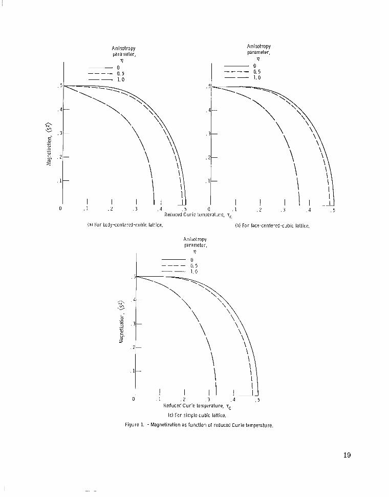
Figure 1. -Magnet izat ion as func t i on of reduced C u r i e temperature.

19

I ( sc) = id' [coth(pQ) + (:r csch2(pQ)coth(pQ) dx" 2' 1 2

where

K; = [ 2V l2 3 - 77 cos(x)

3 - rl cos(x) P =

3

and

3J(k) = [cos(kxa) + cos(k a) + cos(kza)] Y J(0 1

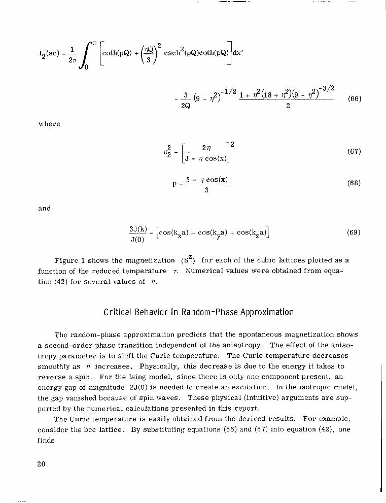
Figure 1 shows the magnetization (Sz) f o r each of the cubic lattices plotted as a function of the reduced temperature T. Numerical values were obtained f rom equa- tion (42) for severa l values of 17.

Cr i t i ca l Behavior in Random-Phase Approximat ion

The random-phase approximation predicts that the spontaneous magnetization shows a second-order phase transition independent of the anisotropy. tropy parameter is to shift the Curie temperature . smoothly as rl increases . Physically, this decrease is due to the energy i t takes to reverse a spin. For the Ising model, s ince there is only one component present, an energy gap of magnitude 2J(O) is needed to create an excitation. the gap vanished because of spin waves. ported by the numerical calculations presented in this report .

consider the bcc lattice. finds

The effect of the aniso- The Curie temperature decreases

In the isotropic model, These physical (intuitive) arguments are sup-

The Curie temperature is easily obtained from the derived results. For example, By substituting equations (56) and (57) into equation (42), one

20

where

and

As Sz approaches zero, t e rms such as Q coth(Q) and Q 3 csch 2 (Q)coth(Q) become

indeterminate. U s e of L'Hospital 's r u l e yields

lim Q coth(Q) = 1 Q-0

and

-2 (7 3)

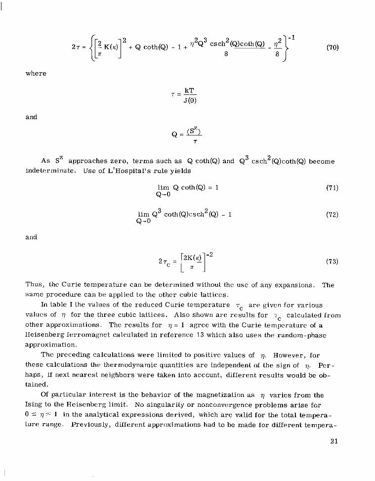
Thus, the Curie temperature can be determined without the u s e of any expansions. s ame procedure can be applied to the other cubic latt ices.

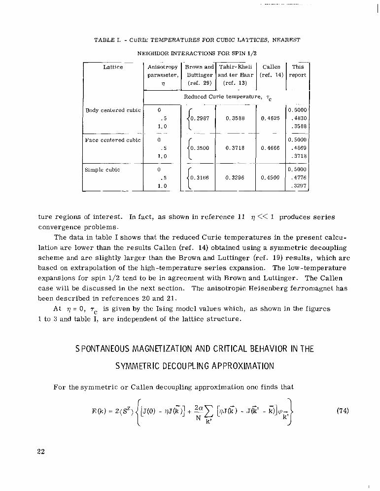
In table I the values of the reduced Curie temperature T~ are given for various values of 17 for the three cubic latt ices. Also shown a r e resu l t s for T~ calculated from other approximations. The resu l t s for r ] = 1 agree with the Curie temperature of a Heisenberg ferromagnet calculated in reference 13 which also u s e s the random -phase approximation.

these calculations the thermodynamic quantities are independent of the sign of r] .

haps, if next nearest neighbors were taken into account, different resu l t s would be ob- tained.

The

The preceding calculations were limited to positive values of 77. However, for Per-

Of particular interest is the behavior of the magnetization as 17 varies f rom the Ising to the Heisenberg limit. 0 5 r ] 5 1 in the analytical expressions derived, which are valid for the total tempera- ture range.

No singularity o r nonconvergence problems arise for

Previously, different approximations had to be made for different tempera-

21

.. - . ._ .. - . ... .. -. .

0.4625

TABLE I. - CURIE TEMPERATURES FOR CUBIC LATTICES, NEAREST

NEIGHBOR INTERACTIONS FOR SPIN 1/2

_ _ 0.5000

.4830

.3588

Lattice

Body centered cubic

_ - Face centered cubic

~

Simple cubic

ture regions of interest . In fact , as shown in reference 11 7 << 1 produces series convergence problems .

The data in table I shows that the reduced Curie temperatures in the present calcu- lation are lower than the resu l t s Callen (ref. 14) obtained using a symmetr ic decoupling scheme and are slightly la rger than the Brown and Luttinger (ref. 19) resul ts , which are based on extrapolation of the high-temperature series expansion. The low-temperature expansions for spin 1/2 tend to be in agreement with Brown and Luttinger. The Callen case will be discussed in the next section. The anisotropic Heisenberg ferromagnet has been described in references 20 and 21.

At q = 0, 7 is given by the Ising model values which, as shown in the figures C

1 to 3 and table I, a r e independent of the lattice s t ructure .

SPONTANEOUS MAGNl3IZATION AND CRITICAL BEHAVIOR IN THE

SYMMETRIC DECOUPLING APPROXIMATION

For the symmetr ic o r Callen decoupling approximation one finds that

f > [J(O) - vJ(G)] + *E [qJG) - JG' - C)]q

k' (74)

22

and

J(k) =c Jgf exp[-z- (g' - 31 f

(75)

By use of equations (A30) and (38), an elementary integration yields the following rela- tion for the correlation function:

where

Thus equation (74) can be replaced by

For the nearest neighbor approximation and constant J,

- - J(k) = J exp(ik - 6) -

6

where is a nearest neighbor vector. It is shown in appendix E that the te rm

[J(C) - J(C - c)]'pk, which appeared in equation (74), can be replaced by

Hence,

1 + 2aqf - J(C) J(O)(rl + 2 0 0

E(k) = 2(SZ)J(0) . - --

(79)

I

where

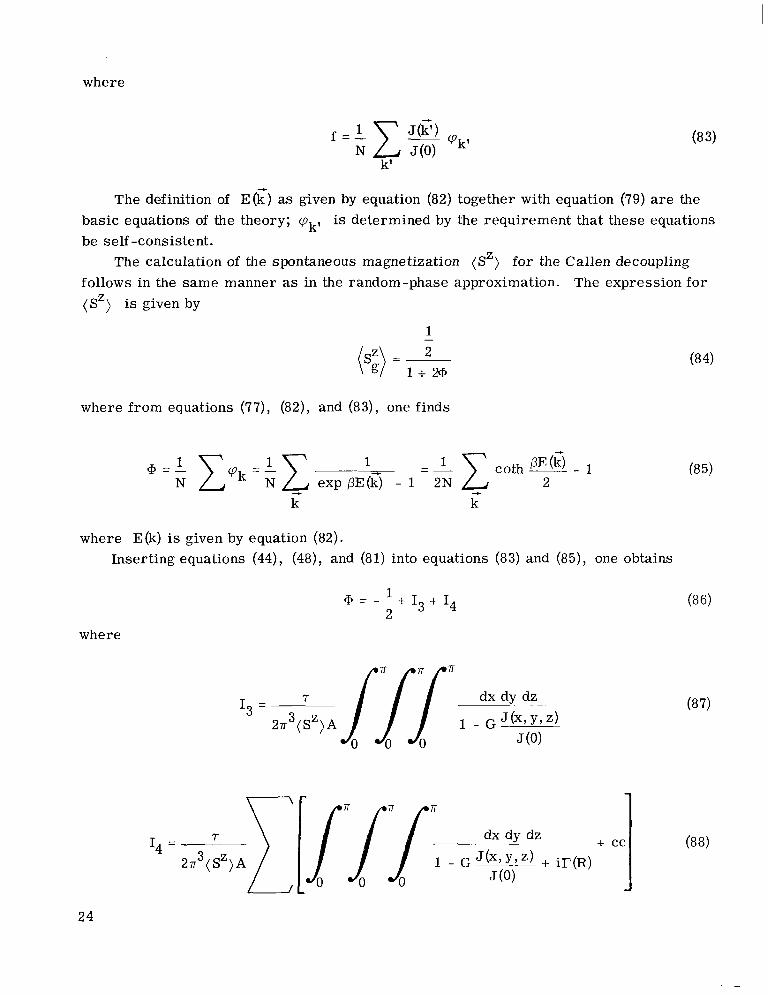
The definition of E(C) as given by equation (82) together with equation (79) are the basic equations of the theory; (pkI is determined by the requirement that these equations be self-consistent.

The calculation of the spontaneous magnetization (Sz) for the Callen decoupling follows in the same manner as in the random-phase approximation. (Sz) is given by

The expression for

1 - 2 (si) =1+29

where from equations (77), (82), and (83), one finds

k k

where E(k) is given by equation (82). Inserting equations (44), (48), and (81) into equations (83) and (85), one obtains

+ = - - + I 1 + I 3 4 2

where

(84)

24

and

A = 1 -C ~ ~ ( 2 f q )

B = q + CY (2f)

B G = - A

where

f = 1 5 + I 6 (9 4)

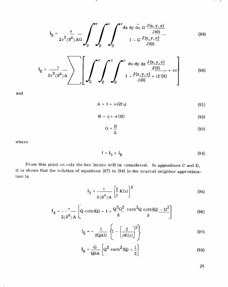
From this point on only the bcc lattice will be considered. In appendixes C and D, it is shown that the solution of equations (87) to (94) in the nearest neighbor approxima- tion is

7 I4 =

2( Sz> A

7 I3 =

2(SZ)A - -

Q coth(Q) - 1 + - Q3G2 csch2Q - coth(Q) - G2 8 8 -

- 2QAG

2 'I I6 = - G [." csch 2 (Q) = -

Q8A

(95)

(9 7)

(98)

25

where K is a complete elliptic integral and

7 i Z Z C r v Callen This report parameter, ’

Curie temperature, T ~ , K 17 ~~.

0.01 Not calculable 0.5

. 5 Not calculable .4970

1.0 0.4625 .4601

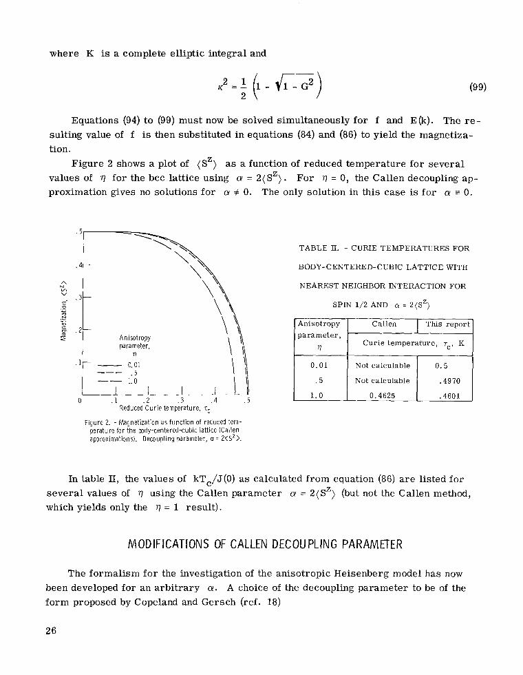
Equations (94) to (99) must now be solved simultaneously fo r f and E(k). The re- sulting value of f is then substituted in equations (84) and (86) to yield the magnetiza- tion.

values of ‘TI for the bcc lattice using cy = 2 ( S z ) . proximation gives no solutions for cy # 0.

Figure 2 shows a plot of (Sz) as a function of reduced temperature for severa l For ‘TI = 0, the Callen decoupling ap-

The only solution in this case is fo r CY = 0.

0 . 1 . 2 . 3 .4 . 5 Reduced C u r i e temperature, -rc

TABLE II. - CURIE TEMPERATURES FOR

BODY-CENTERED-CUBIC LATTICE WITH

Figure 2. - Magnetization as f u n c t i o n of reduced tem- perature fo r t h e body-centered-cubic lattice (Cal len approximations). Decoupling parameter, a = 2<Sz>.

In table II, the values of kTc/J(0) as calculated from equation (86) are listed fo r severa l values of ‘TI using the Callen parameter CY = 2(Sz> (but not the Callen method, which yields only the r ] = 1 resul t ) .

MODIFICATIONS OF CALLEN DECOUPLING PARAMETER

The formalism fo r the investigation of the anisotropic Heisenberg model has now been developed for an a rb i t ra ry cy. A choice of the decoupling parameter to be of the form proposed by Copeland and Gersch (ref. 18)

26

I111

CY = ((2SZ))P

makes it possible to investigate the effect of this parameter on the types of transitions and Curie points fo r various positive powers p. The case p = 1 is jus t the ordinary Callen decoupling which has already been discussed.

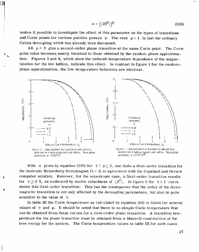
point value becomes nearly identical to those obtained by the random -phase approxima- tion. tization fo r the bcc lattice, indicate this effect. In contrast to figure I for the random- phase approximation, the low-temperature behaviors are identical.

All p 1 3 give a second-order phase transition at the s a m e Curie point. The Curie

Figures 3 and 4, which show the reduced-temperature dependence of the magne- e

%

I

0 . 1 . 2 . 3 . 4 . 5 0 . I . 2 . 3 . 4 . 5 Reduced C u r i e temperature, TC

Figure 3. -Magnet iza t ion as f u n c t i o n of reduced tem-

Reduced C u r i e temperature, T~

perature fo r a b d y - c e n red cub ic lattice. Decoupling parameter, a = ( z < s ~ > I .

F igure 4. - Magnetization as func t ion of reduced tem-

16 - perature for a body-ce ered-cubic lattice. Decoupling parameter, a = (2(sZ)) 9 .

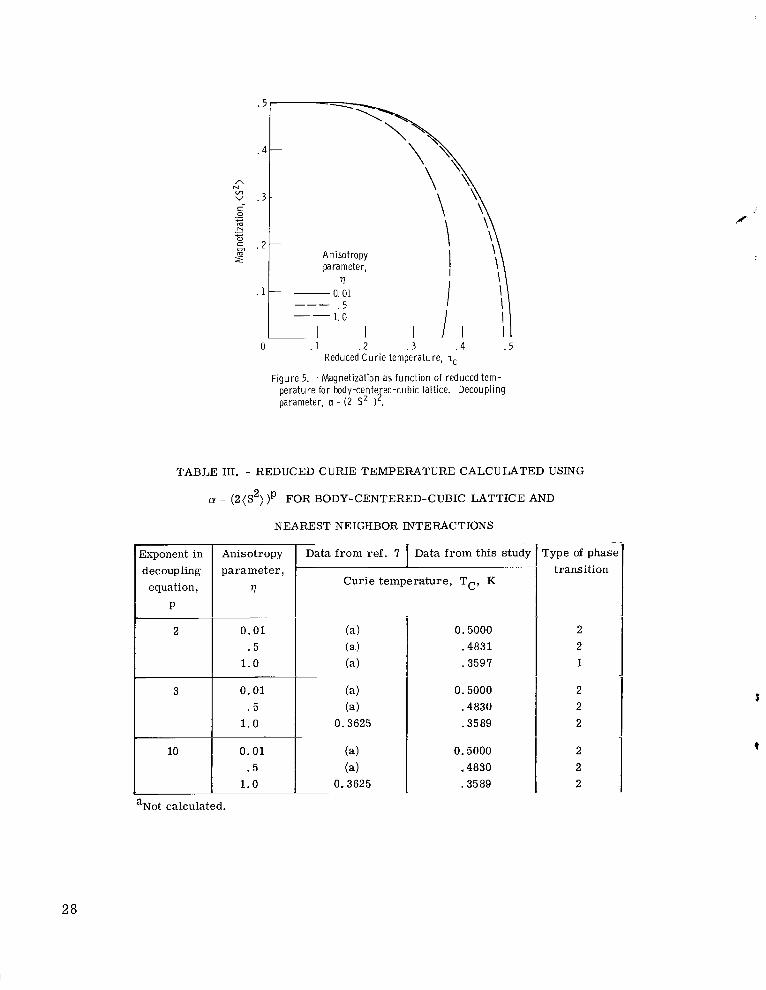
With CY given by equation (100) for 1 < p s 3 , one finds a f i r s t -order transition for the isotropic Heisenberg ferromagnet ( q = 1) in agreement with the Copeland and Gersch computer solution. for q 2 0.5 , as evidenced by double valuedness of (S') . In figure 5 the q = 1 curve shows this f irst-order transition. magnetic transition is not only affected by the decoupling parameters , but also is quite sensitive to the value of q.

In table 111 the Curie temperature as calculated by equation (84) is listed f o r severa l values of rl and p. It should be noted that there is no simple Curie temperature that can be obtained from these curves fo r a first-order phase transition. A transition t em- perature for the phase transition must be obtained from a Maxwell construction of the free energy for the sys tem. The Curie temperature values in table 111 f o r such cases

F However, fo r the anisotropic case , a f i r s t -order transition results

This has the consequence that the o rde r of the f e r r o - +

27

I. -

! "I

Anisotropy parameter,

i

. 1

1. 0 --

I 0 . 1 .2 . 3 . 4 . 5

Reduced C u r i e temperature, T~

F igu re 5. -Magnet izat ion as func t i on of reduced tem- perature for body-cente ed cub ic lattice. Decoupling parameter, a = (2 S' f - .

TABLE 111. - REDUCED CURIE TEMPEMTURE CALCULATED USING

cy = (2(S2))p FOR BODY-CENTERED-CUBIC LATTICE AND

NEAREST NEIGHBOR INTERACTIONS

1.0

1.0

10 0.01 .5

1.0

~

Data from ref. 7 Data from this study

Curie temperature, TC, K I ~

0.5000 .4831 .3597

0.5000 .4830 .3589

0.5000 .4830 .3589

rype of phasc transition

2 2 1

2 2 2

2 2 2

aNot calculated.

28

are the intercepts of the (S’) curve on the temperature axis.

f o r a . There is no unique way to determine LY within the Green’s function formalism, and thus one must re ly on experimental observations for this information.

ferromagnetic transition. Inhomogeneity of the concentration, that is, nonuniform dis - tribution, of impurities may lead to the appearance of a tail on the curve of the sponta- neous magnetization. The ferromagnetic transition can occur, therefore, not at a single temperature but over a range of temperatures. One possible reason for this tail is that the inhomogeneity of the concentration leads to regions in the mater ia l which have different Curie temperatures. In those regions of the specimen having a higher Curie temperature, the spontaneous magnetization is still re- tained when a pa r t of the ferromagnetic mater ia l has gone over into the paramagnetic phase (ref. 22). s e rve as a measure of inhomogeneity.

developed that had the form

The formalism has been developed up to this point fq r an a rb i t ra ry functional fo rm

Structural characterist ics of the mater ia l have strong effects on the nature of the

Thus, the transition is smeared out.

It is suggested, therefore, that the anisotropy parameter can, in effect,

In the section MODIFICATIONS OF THE DECOUPLING PARAMETERS a model was

CY = (2(SZ))P + (2( SZ))P log(Z(SZ))1’

If equation (101) is used in conjunction with equation (74), one finds the following resu l t s :

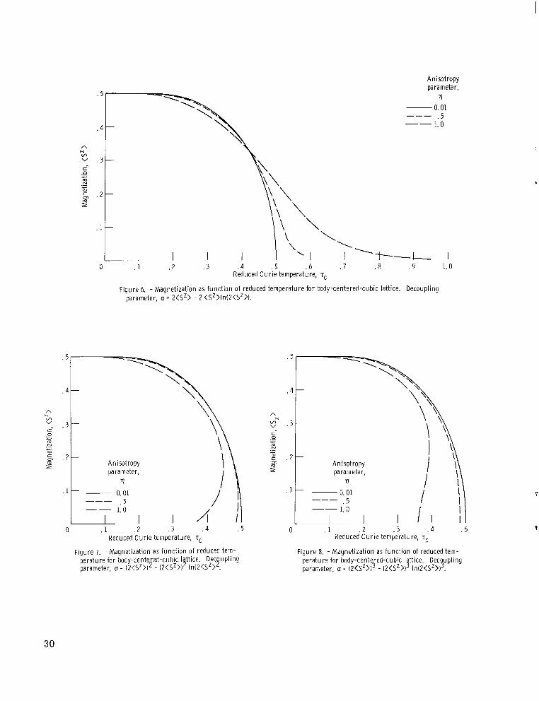
Fo r p = 1 (fig. 6) , a washed-out transition is obtained. For p = 2 (fig. 7) the isotropic Heisenberg model ( q = 1 .0 ) gives a f i r s t -order

transition; whereas, for sma l l q one obtains a second-order transition. This c o r r e - sponds closely to the p = 2 case for the Callen exponential decoupling.

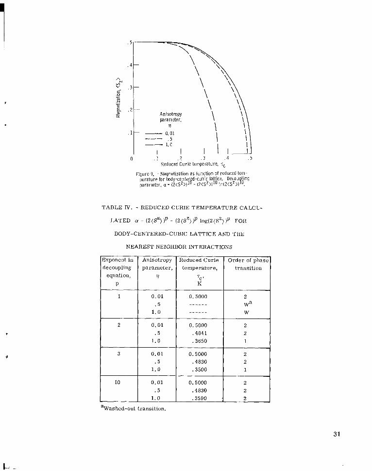
For p = 3 an important effect comes into play. Previously the exponential Callen decoupling parameter (eq. (100)) gave only a second-order phase transition for q 2 0, as well as the same Cur ie temperature independent of the p. approximation, the order of the phase transition depends on p. For p = 3 (fig. 8) the isotropic Heisenberg model (q = 1.0) produces a f i r s t -order transition; whereas for sma l l 17 a second-order transition results. However, for p = 10 (fig. 9) only a second-order transition is present. value for the Curie temperature. occur when the decoupling scheme (eq. (101)) is used.

Table IV gives the reduced Curie temperatures fo r this decoupling parameter fo r the bcc lattice. The W means that a washed-out transition occurs. Experimentally, it is difficult to distinguish between a higher order and a truly washed-out transition.

Fo r the present decoupling

T

F o r q = 0 there is no change in the Ising model t Figures 8 and 9 i l lustrate that various transitions

29

Anisotropy parameter,

rl 0.01 . 5

1.0 --- --

Reduced C u r i e temperature, T~

F igure 6. - Magnetization as f u n c t i o n of reduced temperature fo r body-centered-cubic lattice. Decoupling parameter, a = 2<s2> - 2 < s ~ > I ~ ( ~ < s ~ > ) .

- Anisotropy para meter,

7

0. 01 . 5

1.0

-

__-

. 5

--

. 1 . 2 . 3 .4 I I

Reduced C u r i e temperature, T~

Fioure 7. - Maqnetization as f u n c t i o n of reduced tem- perature for b d y - c e n t e ed cub ic Igttice. Oec2upling parameter, a = (2<Sz>)J - i2<5z>) In(2<Sz> .

A

v, v

N

c 0

m N

a, c in

.- -

.- c

1

/ I ‘ I I 1. 0 --

I 0 . 1 . 2 . 3 .4 . 5

Reduced C u r i e temperature, T~

Figure 8. -Magnet iza t ion as func t ion of reduced tem- pera ture for body-cente ed cubic lattice. Decoupling pararr,eter, a = (2<5z>$ - i < s z > ) 3 ln(2<Sz>)3.

7

30

r

Exponent in decoupling

equation, P

1

2

3

0 . 1 . 2 . 3 . 4 . 5 Reduced Cur ie temperature, T~

Figure 9. - Magnetization a s func t ion of reduced tem- perature for body-centered-cubic lattice. Decou ling parameter, a = ( ~ < S Z > ) ~ O - ( ~ < S Z > ) ~ O \n(2<SZ>)'O.

Anisotropy parameter,

17

0.01 . 5

1.0

0.01 . 5

1.0

0.01 . 5

TABLE N . - REDUCED CURIE TEMPERATURE CALCU-

LATED cy = (2(SZ))' - (2(Sz))p log(Z(Sz>)p FOR

BODY-CENTERED-CUBIC LATTICE AND THE

NEAREST NEIGHBOR INTERACTIONS

pT--t-+ 1 . 0

Reduced Curie temperature,

'C ' K

0.5000 .4841 .3650

0.5000 .4830 .3500

0.5000 .4830 .3590

Order of phase transition

aWashed-out transition.

31

CON CLU S I ON S

From the results obtained by the use of Green's functions and various decoupling schemes, certain conclusions can be stated:

1. A single analytical expression for magnetization, which is valid for all tempera- tu res , was obtained. The demonstrated technique of evaluating cer ta in Watson sums and integrals was employed without requiring various series approximations o r extensive computer summations. Other thermodynamic quantities, such as specific heat, can be calculated from the magnetization.

shows a second-order phase transition at Curie temperature (a discontinuity in the slope of the magnetization and in the second derivative of the free energy) independent of the anisotropy. perature . increases .

3. The Callen approximation for spontaneous magnetization produces self -consistent

2. The random -phase approximation predicts that the spontaneous magnetization

The effect of the anisotropy parameter is to shift the cr i t ical (Curie) tem- The curie temperature decreases monotonically as the anisotropy parameter

field equations that predict a second-order phase transition. shifts the Curie temperature. than those obtained by the random phase approximation.

4. The exponential decoupling parameter for 1 < p < 3 predicts, by the use of self- consistent field equations, a f i rs t -order transition for large values of anisotropy param- eter q and a second-order phase transition for small values. The type of phase t ransi- tion is sensitive to the value of the anisotropy parameter . For p 2 3 (where p is any power), a second-order transition is obtained whose reduced Curie temperature is in close agreement with the random -phase approximation. of magnetization is not the same as that predicted by the random-phase approximation.

to the value of anisotropy parameter . For example, for p = 10 a washed-out transition j s obtained. But for p = 3 the Heisenberg model gives a f i r s t -order transition for large values of q and a second-order transition for smal l values. In contrast , p = 2 shows the reverse situation. For p = 1 and n = 1, a washed-out transition is obtained. For q < 1, the behavior is that of either a washed-out o r higher order phase transition.

The anisotropy parameter The values of the reduced Curie temperature a r e higher

The low-temperature dependence

5. The logarithmic decoupling parameter shows what type of transition is sensitive

Lewis Research Center, National Aeronautics and Space Administration,

Cleveland, Ohio, June 30, 1970 , 129-02.

32

APPENDIX A

REVIEW OF GREEN'S FUNCTION

The Green's function method allows one to focus attention on the quantity of interest and to determine from the complete Hamiltonian the exact coupled equations of motion fo r the associated Green's function. In order to solve these equations they must be truncated or uncoupled by a suitable decoupling approximation. Although the usual de- coupling approximations are not now well understood, this method is a convenient tech- nique for the calculation of various thermodynamic quantities as a function of tempera- ture .

r

"

In this review, the propert ies of the temperature -dependent double -time Green's function are studied in relation to the work presented in this report . treatments of the problems may be found in general review ar t ic les and books, such as those by Zubarev (ref. 4), Bonch-Bruevich and Tyablikov (ref. 23), Kadanoff and Baym (ref. 24), and Pe r ry and Turner ( ref . 25).

More standard

Causal Retarded and Advanced Green's F u n c t i o n

For a system with a time independent Hamiltonian H, the causal re tarded and ad- vanced Green's function for a pair of operators A and B are defined as follows:

Gc(t , t') = ((A(t) ; B(t '))) = -i(TA(t)B(t ')) (AI)

GA(t, t ' ) = ( (A( t ) ; B(t ' ))) = ie(t ' - t ) ( [ A ( t ) , B(t')]) (A 3)

.l where A(t) is the Heisenberg representation for the operator A ,

A(t) = exp(AHt)A exp(-hHt) 't

and T is the t ime ordering operator of Dyson, which is defined in the usual way s o that

with Q(t) as the s tep function,

33

I I

+1 [A, B] = AB - uBA: o =

-1

Note that A and B are not res t r ic ted to be either Bose o r F e r m i operators and that the choice of (J is arb i t ra ry . For the case of Bose operators that are used herein, (J = 1 and the singular angular bracket denotes the average with respec t to the canonical density matrix of the system

where

and

Using the equation of motion

p = - 1 kT

- - idA - [A,H] = AH - HA d t

and the property of the step function

resu l t s in

and similarly f o r the causal and advanced Green's function. tion on the right side of the equation can be of higher order than on the left. Writing down

34

Note that the Green's func-

the equations of motion for the higher order functions, a set of coupled equations for the complete hierarchy of Green's function can be obtained. It is easily shown that the Green's function G(t , t') can be written in the form G(t - t '), and thus depends only on the time difference.

The t ime correlation function plays an important role in statistical mechanics and is usually the quantity of d i rec t physical interest . It is written as

which can be calculated from equations (15), (16), and the cyclic property of the t race.

SPECTRAL REPRESENTATION

To obtain the spectral r epesen ta t ion of the time correlation functions the eigen- function m and eigenvalues EFl of the Hamiltonian must be considered. Thus

From equation (A14), the correlation function can be written

- T r [exp( -PH)exp( -iHt' )B exp(iHt)A] - ~.

T r exp(-OH)

= Z -1 (mlBln)(nlAlm)exp(-Emp)exp - [i(Em - En)(t ' - t)] m7n

with

the partition function for the canonical ensemble. following manner:

Equation (23) can be rewrit ten in the

35

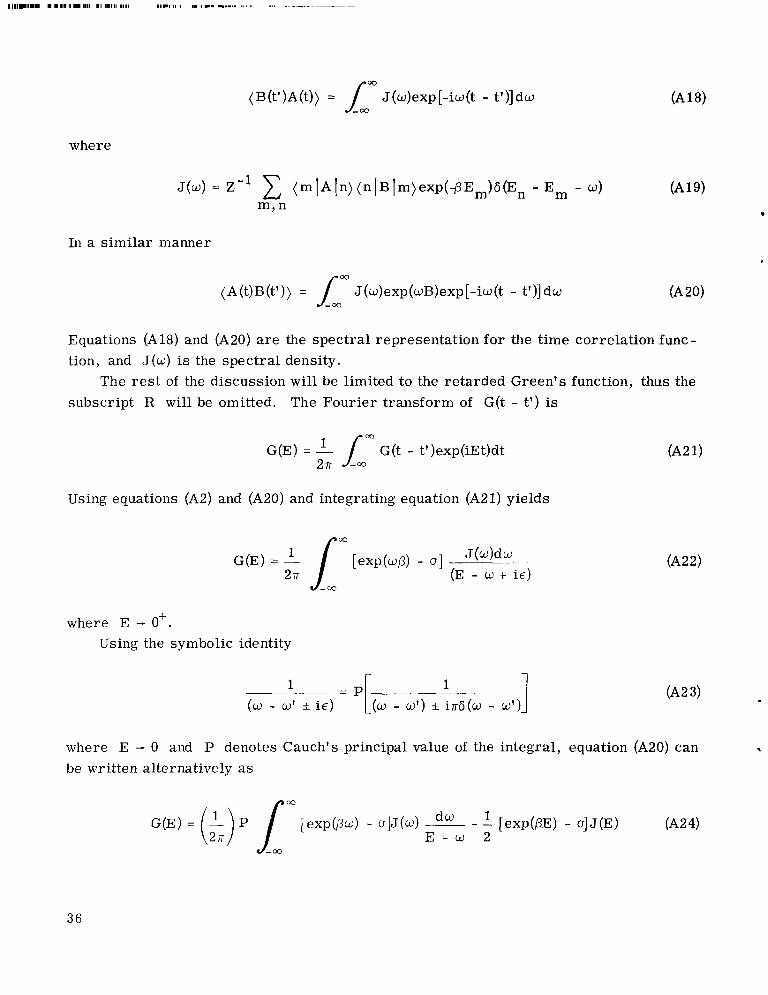
03

(B(t')A(t)) = / J(w)exp[-iw(t - t')]dw -Q)

where

In a s imi la r manner

(A(t)B(t')) = f J(w)exp(wB)exp[-io(t - t ')]do -a3

Equations (A 3) and (A20) are the spec t ra l representation f o r the t ime c o r r e d i o n func- tion, and J ( w ) is the spec t ra l density.

The rest of the discussion will be limited to the re ta rded Green's function, thus the subscript R will be omitted. The Fourier transform of G(t - t') is

G(E) = - ' 2 n

G(t - t ')exp(iEt)dt

Using equations (A2) and (A20) and integrating equation (A21) yields

J(w)dw (E - w + ic)

G(E) = - 2T

where E - O+. Using the symbolic identity

where E - 0 and P denotes Cauch's principal value of the integral, equation (A20) can 3

be written alternatively as

J- 03

3 6

I

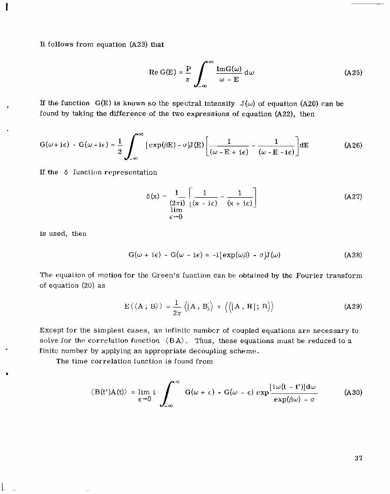
It follows from equation (A23) that

Re G(E) = - lmG(w) d w 7r 1 w - E

d- 00

If the function G(E) is known s o the spectral intensity J ( w ) of equation (A20) can be found by taking the difference of the two expressions of equation (A22), then

3

If the 6 function representation

6(x) =-

lim E -0

is used, then

G(w + ie) - G(w - ic) = -i[exp(wp) - a ] J (w) (A2 8)

The equation of motion for the Green's function can be obtained by the Fourier transform of equation (20) as

Except for the simplest cases , an infinite number of coupled equations are necessary to solve for the correlation function ( B A ) . finite number by applying an appropriate decoupling scheme.

Thus, these equations must be reduced to a

The time correlation function is found from

37

APPENDIX B

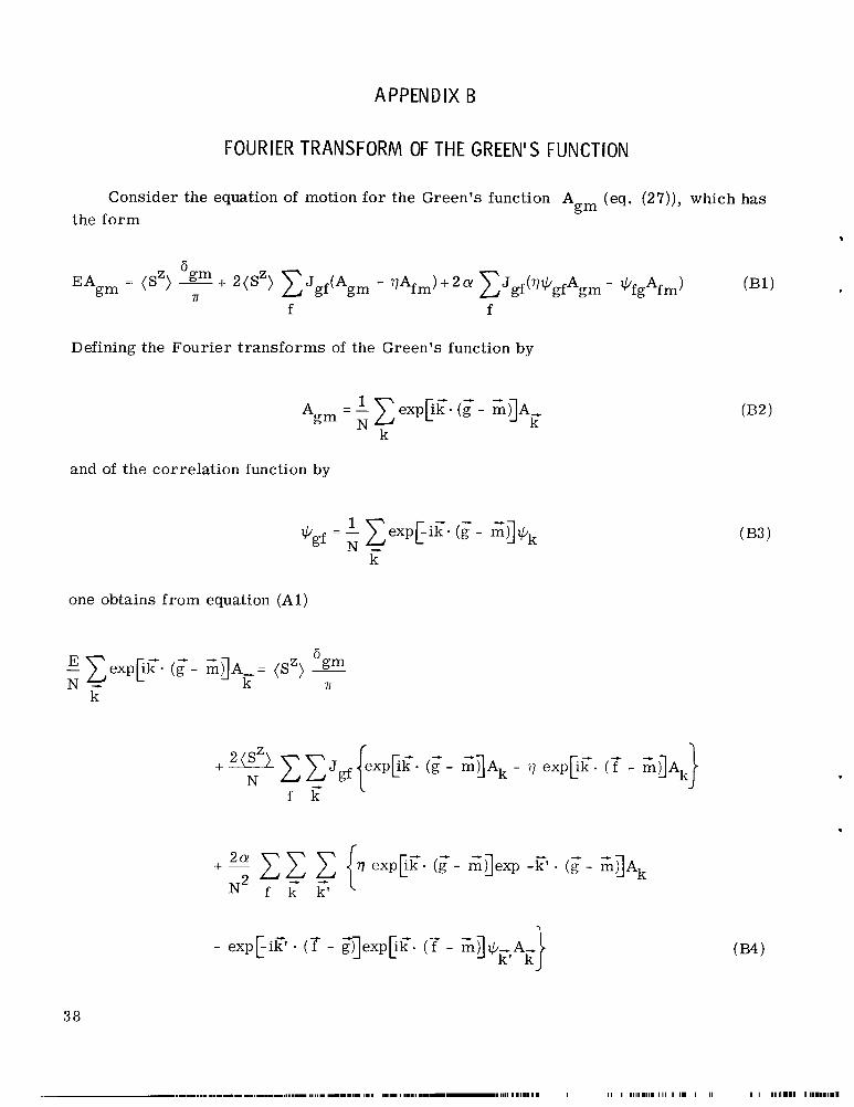
FOURIER TRANSFORM OF THE GREEN'S FUNCTION

Consider the equation of motion fo r the Green's function A (eq. (27)), which has gm

the fo rm *

f f

Defining the Fourier t ransforms of the Green's function by

and of the correlation function by

one obtains f rom equation ( A l )

38

.-.-....-,..---,-.. ,.,,..I.. -.11111.- 1 . 1 1 - 1 1 1 1 . 1 11.1 1,111 I m.II.1I-11111 1111111111 I I1 I 1111111111 1 1 1 I 111 1- I1 I I 111111111 1111111111.1

I

If equation (B4) is multiplied by

and if the following relations a r e used

39

then

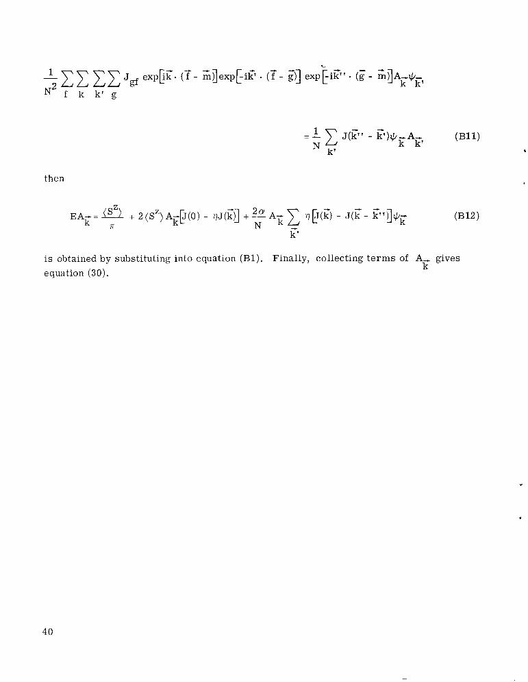
is obtained by substituting into equation ( B l ) . equation (30).

Finally, collecting t e r m s of A, gives k

40

.

APPENDIX C

EVALUATION OF INTEGRALS 11

Body-Centered -C ubic Latt ice

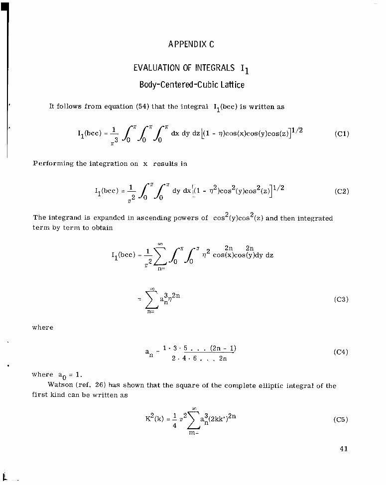
It follows f rom equation (54) that the integral Il(bcc) is writ ten as

Performing the integration on x resu l t s in

I (bcc) = 1 f ITLIT dy d x l l - 'q2)cos2(y)cos2(z)]1'2 1 2 0 IT

The integrand is expanded in ascending powers of cos 2 (y)cos 2 (z) and then integrated

t e r m by t e r m to obtain

cu 2n 2n

I (bcc) = IT IT^' 'q2 cos(x)cos(y)dy dz 2 1

IT n=

where

- 1 . 3 . 5 . . . ( 2 n - 1) 2 . 4 - 6 . . . 2n an -

where a. = 1.

first kind can be written as Watson (ref. 26) has shown that the square of the complete elliptic integral of the

m

K 2 (k) = I 1 ~ ~ 2 ~ ( 2 k k ~ ) ~ " n 4

(C5)

41

m=

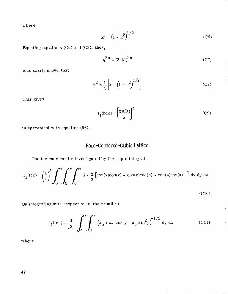
where

k’ = (1 - k2)1/2

Equating equations (C5) and (C3), thus,

it is easily shown that

This gives

2 Il(bcc) = [y]

in agreement with equation (56).

Face-Centered-Cu b ic Lattice

The fcc case can be investigated by the t r iple integral

(C10)

On integrating with respect to x the result is

- 1/2 I1(fcc) = - l’ln (ao + al cos y + a5 s in 2 y) dy dz 2

T T j

where

42

Let

Then,

I -2(1 + 3, cos(z) a1 = ---T

2 a5 = sin (2)

t = tan(.)

dy = (1 + t 2 )dy

1 - tan2 cos(y) =

1 + tan'(:) 1 + t 2

2t

If these relations are substituted into equation ( C l l ) , then

- 1/2 Il(fcc) = 2[(r2q)] f 'Im (bo)-1'2 (A + Bt2 + t") dt dz

0 0

where R

b o = ( a 0 1 - a )

a + al 0 A =

and

43

If

2 B2 - 4A < + = B 2 +

B2 - 4A - 2 5 = B 2 -

then

- 1/2 dt dz (C23) I1(fcc) = [2(iT2?7)] /" /- (bo)- 1/2 [(- 2 + r+)(t 2 2 + czj]

0 0

Once the radical has been expressed in this factored form as the product of sums o r differences of squares , the integral can be reduced to Jacobian o r elliptical form. integral of (C23) is finite everywhere and leads to the integral of the f i r s t kind. f rom elementary tables

The Thus,

where

Some algebraic manipulation gives

which is the s a m e as equation (60).

44

Simple-Cubic Lattice

The integral for the s c lattice in three dimensions can be written as

I 1 (SC) = LL’jT 3 dx dy d z { J A 3 [coS(X) + coS(y) + cOS(Z)] r1 (C27)

0 0 71

The s a m e procedure that was outlined in the previous section gives for the fcc case:

I1(sc) = - /” <[3 - 77 cos(z)]K(k2)dz 2 0

71

where

k i = [ 2rl 3 - 17 cos(z)

which is of the s a m e form as in equation (65).

45

APPENDIX D

SUMMATION AND THE LAPLACE TRANSFORM

The calculation of the integral I2 involves the summation of a n infinite series. A direct approach to the problem of the summation of infinite series has been given by several authors (refs. 27 and 28). evaluate 12.

As an example of the technique used, consider the fcc lattice. (The calculation for the other two cubic latt ices follow in the s a m e manner): the fcc lattice integral is wr i t - ten as

Some of these techniques will be used and extended to

3

n3Q

12(fcc) = - 11 R= 1

where

dz

3J(x9 y, z, = cos(x)cos(y) + cos(y)cos(z) + cos(z)cos(x) J(0)

The t r iple integration and the summation exist and a r e real. However, they can be writ ten as the difference of two complex integrals as was done in equation (52). Inte- grating on x and y (appendix D) gives

dz L 3 + a + 3 i r ( R )

R= 1

where

4?7[3 + q cos2(z) + 3ir(R)] - - . . - . . . 12 k, =

1 [3 + q + 3ir(R)12

46

RTi r ( R ) = - Q

and cc indicates the complex conjugate. The complete elliptic integral of the f i r s t kind can be represented in series f o r m as

where

K(k) = - 2 71 1 a:k2n lkl < 1

n

1 . 3 . 5 . . . ( 2 n - 1 ) a = 1 - - -

an - 2 - 4 . 6 . . . 2n 0

Only the f i r s t two t e r m s of the s e r i e s in equation (D7) a r e necessary for four place ac- curacy.

respect to z, the t e r m s can be rearranged to show that

There is no difficulty in extending it to as many t e r m s as needed. Taking the f i r s t two t e r m s in equation (D3) and integrating the complex function with

12(fcc) = $ + I2 b c + I2

where

1; = (177)

y2 + R2 R= 1

2 - n G I b -

R= 1

1 2R2 I

I ly2 + R2 (y2 + R2Y]

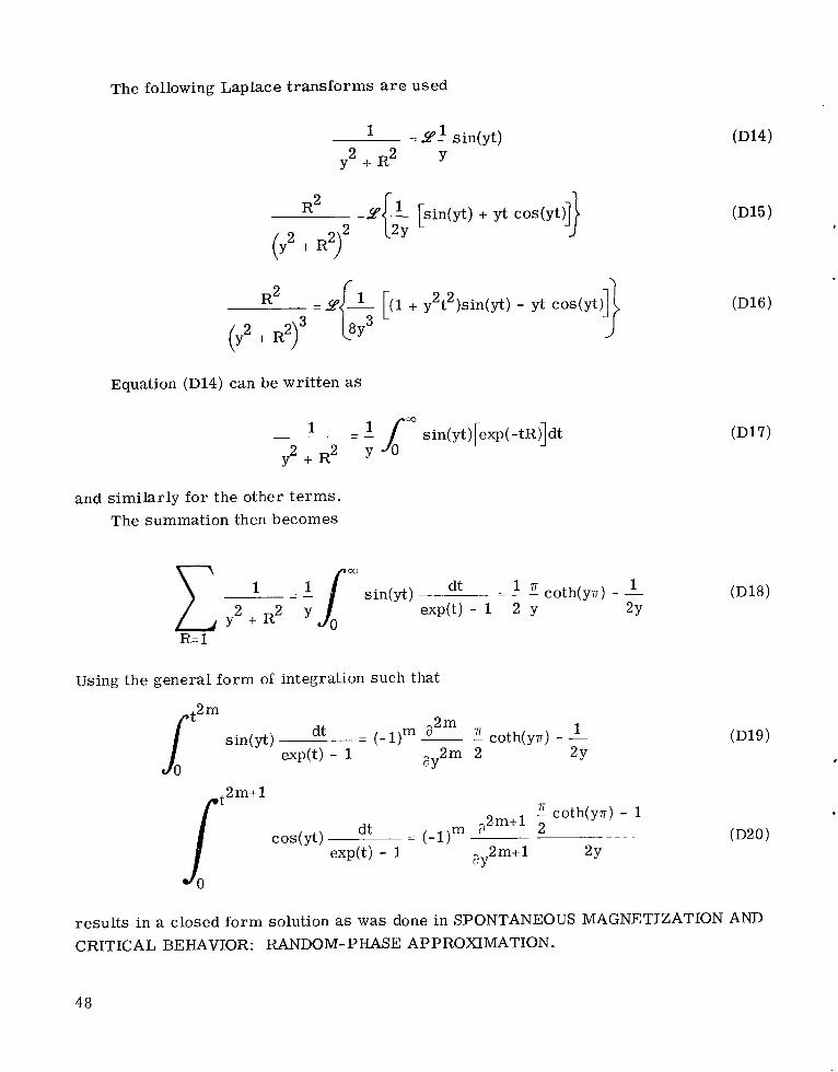
The following Laplace t ransforms are used

=Y- 1 sin(yt)

y2 + R2 Y

Equation (D14) can be writ ten as

= 1 /" sin(yt)[exp(-tR)ldt y2 + R2

and s imilar ly for the other t e rms . The summation then becomes

Using the general form of integration such that

t2 m+ 1 1 coth(y7r) - 1 2m+l

dt = (-1) m i , ~. . cos(Yt) exp(t) - 1 ay2m+l 2Y

resu l t s in a closed fo rm solution as was done in SPONTANEOUS MAGNETIZATION AND CRITICAL BEHAVIOR: RANDOM- PHASE APPROXIMATION.

48

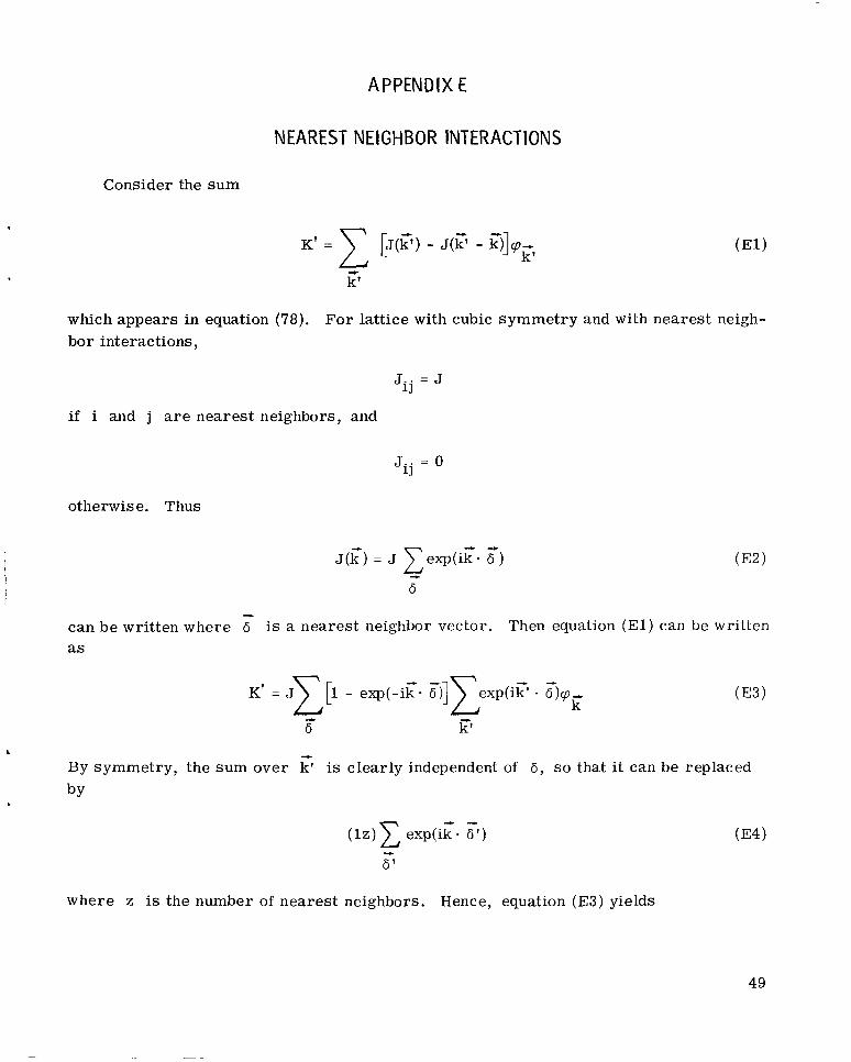
APPENDIX E

NEAREST NE1 GH BOR INTERACTIONS

Consider the s u m

which appears in bor interactions,

K' = 7 [J(C) - J(C - c)]~p-+~

equation (78). For latt ice with cubic symmetry and with nearest neigh-

J.. = J 1.l

if i and j are nearest neighbors, and

J.. = 0 1.l

otherwise. Thus

- can be written where 6 is a nearest neighbor vector. as

Then equation ( E l ) can be written

L - By symmetry, the sum over k' is clearly independent of 6 , so that i t can be replaced by

- - ( l z ) E exp(ik - 6 ' ) -

6'

where z is the number of nearest neighbors. Hence, equation (E3) yields

49

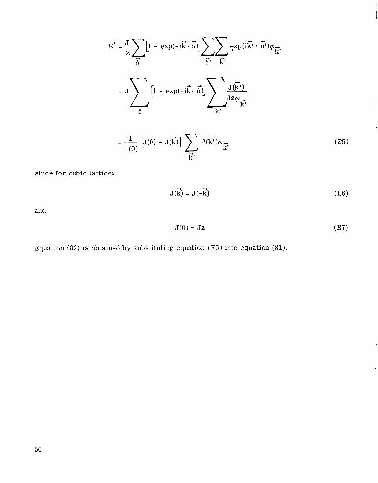
since f o r cubic lattices

6 k'

J(Z) = J(-C)

and

J ( 0 ) = JZ

Equation (82) is obtained by substituting equation (E5) into equation (81).

50

REFERENCES

1. Weiss, P. : Hypothesis of the Molecular Field and Ferromagnetism. J. Physique, vol. 6, Sept. 1907, pp. 661-690.

2. Heisenberg, W. : Zur Theorie des Ferromagnetismus. Zei t . f . Physik, vol. 49, no. 9-10, July 16, 1928, pp. 619-636.

3. Dirac, P. A. M. : Quantum Mechanics of Many-Electron Systems. P roc . Roy. SOC. (London), Ser. A, vol. 123, no. 792, Apr. 6, 1929, pp. 714-733.

4. Zubarev, D. N. : Double-Time Green Functions in Statistical Physics. Soviet Phys. Uspekhi, vol. 3, no. 3, Nov.-Dec. 1960, pp. 320-345.

5. Bogolyubov, N. N. ; and Tyablikov, S. V. : Retarded and Advanced Green Functions in Statistical Physics. Soviet Phys. -Doklady, vol. 4, no. 3, Dec. 1959, pp. 589- 593.

6. Ising, Erns t : Beitrag zu r Theorie des Ferromagnetismus. Zeit. f . Physik, vol. 31, 1925, pp. 253-258.

7. Onsager, L a r s : Crys ta l Statistics. I. A Two-Dimensional Model with an Order- Disorder Transition. Phys. Rev., vol. 65, no. 3-4, Feb. 1-15, 1944, pp. 117- 149.

8. Horwitz, Gerald; and Callen, Herbert B. : Diagrammatic Expansion for the Ising Model with Arbi t ra ry Spin and Range of Interaction. Phys. Rev., vol. 124, no. 6, Dec. 15, 1961, pp. 1757-1785.

9 . Baker, George A. , J r . ; Rushbrooke, G. S. ; and Gilbert, H. E . : High-Temperature Series Expansions fo r the Spin-1/2 Heisenberg Model by the Method of Irreducible Representations of the Symmetric Group. Phys. Rev., vol. 135, no. 5A, Aug. 31, 1964, pp. 1272-1277.

10. Baker, George A. , Jr. ; and Gaunt, David S. : Ising-Model Cri t ical Indices Below the Cri t ical Temperature. Phys. Rev., vol. 155, no. 2, Mar. 10, 1967, pp. 545- 552.

11. Dalton, N. W. ; and Wood, D. W. : Crit ical Behaviour of the Simple Anisotropic Heisenberg Model. Proc . Phys. SOC., vol. 90, pt. 2, Feb. 1967, pp. 459-474.

12. Oguchi, Takehiko: Theory of Spin-Wave Interactions in F e r r o - and Antiferromag- netism. Phys. Rev., vol. 117, no. 1, Jan. 1, 1960, pp. 117-123.

13. Tahir-Kheli, R. A. ; and ter Haar, D. : Use of Green Functions in the Theory of Ferromagnetism. I. General Discussion of the Spin-S Case. Phys. Rev., vol. 127, no. 1, July 1, 1962, pp. 88-94.

51

14. Callen, Herbert B. : Green Function Theory of Ferromagnet ism. Phys. Rev. , vol. 130, no. 3, May 1, 1963, pp. 890-898.

15. Tyablikov, Sergei V. : Methods in the Quantum Theory of Magnetism. Plenum Press, 1967.

16. Raich, J. C. ; and Et te rs , Richard D. : Elementary Excitations in fcc Solid Ortho- Hydrogen. Phys. Rev. , vol. 168, no. 2, Apr. 10, 1968, pp. 425-436.

17. Flax, Lawrence: Theory of Phase Transit ions in Solid Hydrogen. Presented at the American Physical Society Meeting on Quantum Theory of Solids, Aspen, Colo. , Sept. 1-5, 1969.

18. Copeland, J. A. ; and Gersch, H. A. : Firs t -Order Green's-Function Theory of the Heisenberg Ferromagnet. Phys. Rev., vol. 143, no. 1, Mar. 1966, pp. 236-244.

19. Brown, H. A. ; and Luttinger, J. M. : Ferromagnetic and Antiferromagnetic Curie Temperatures . Phys. Rev., vol. 100, no. 2 , Oct. 15, 1955, pp. 685-692.

20. Flax, Lawrence; and Raich, John C. : Calculation of the Generalized Watson Sums with an Application to the Generalized Heisenberg Ferromagnet. vol. 185, no. 2 , Sept. 10, 1969, pp. 797-801.

Phys. Rev. ,

21. Flax, Lawrence; and Raich, John C. : Random Phase Approximation for the Aniso- tropic Heisenberg Ferromagnet. NASA T N D-5286, 1969.

22. Belov, Konstantin P. (W. H. Fur ry , t rans . ): Magnetic Transitions. Consultants Bureau, 1961.

23. Bonch-Bruevich, V. L. ; and Tyablikov, S. V. : The Green Function Method in Sta- t ist ical Mechanics. Interscience Publ. , 1962.

2 4 . Kadanoff, Leo P. ; and Baym, Gordon: Quantum Statist ical Mechanics. W. A. Benjamin, Inc., 1962.

25. Parry, W. E . ; and Turner , R. E. : Green Functions in Statistical Mechanics. Rep. P rogr . Phys . , vol. 27, 1964, pp. 23-52.

26. Watson, G. N.: Three Triple Integrals. Quart . J. Math., vol. 10, 1939, pp. 266- 1

276.

27. Wheelon, Albert E. : On the Summation of Infinite Ser ies in Closed Form. J. Appl. Phys . , vol. 25, no. 1, Jan. 1954, pp. 113-118.

28. Mannari, Isao; and Kageyania, Hiroko: A Note on Extended Watson Integrals. P rogr . Theoret. Phys. Suppl. Extra Number, 1968, pp. 269-279.

52 NASA-Langley, 1970 - 26 E-5715

__. , -

NATIONAL AERONAUTICS AND SPACE ADMINISTRATION WASHINGTON, D. C. 20546

OFFICIAL BUSINESS FIRST CLASS MAIL

POSTAGE A N D FEES PAID NATIONAL AERONAUTICS AND

SPACE ADMINISTRATION

I O U 001 51 51 3us 70272 00903

A J K F O R C E WEAPONS L A B O R A T O R Y / W L O L / KIRTLAND AFB, NEW MEXICO 87117

A T 1 E. L U U B O W M A N , CHIEFVTECH. L I B R A K V

POSTMASTER: If Undeliverable (Section 158 Postal Manual) Do Nor Return

-. _. .

‘The aeroizniitical niad spnce activities of the United Stntes shull be conducted so ns t o coiztribzite . . . t o the expnnsion of himaiz. kiaoiul- edge of phenomeiza in the ntuiosphere nizd space. The Adiiiiiaistration shrill proi’ide fo r the widest pimticnble and npproprinte disseniimtiou of iizfori)intion cotzceruiizg its nctittities nizd the re sd t s thereof.”

-NATI&A:~ A.E’RS)NAUTICS AND SPACE ACT OF 193s :z

. I

NASA SCIENTIFIC AND TECHNICAL PUBLICATIONS . ,

...e. . . ....

TECHNICALkEPORTS: Scientific and ’ TECHNICAL TRANSLATIONS: Information technical information considered important,: . complete, and .a.lasting contribution to e x i d n g knowledge.

TECHNICAL NOTES: Information less koad in scope but nevertheless of importance as$ .’; contribution to existing knowledge.

TECHNICAL MEMORANDUMS: Information receiving limited distribution ,,;, TECHNOLOGY UTILIZATION because of preliminary data, securitp:.~lassifica- tion, or other reasons.

CONTRACTOR REPORTS: Scientific and .

technical information generated under a NASA contract or grant and considered an important contribution to existing knowledge.

published in a foreign language considered to merit NASA distribution in English.

SPECIAL PUBLICATIONS: Information derived from or of value to NASA activities. Publications incliide conference proceedings, monographs, data compilations, handbooks, sourcebooks, and special bibliographies.

/ . . . .

.. .. . .

PUBLICATIONS: Information on technology used by NASA that may be of particular interest in commercial and other non-aerospace applications. Publications include Tech Briefs, Technology Utilization Reports and Notes, and Technology Surveys.

Details on the availability of these publications may be obtained from:

SCIENTIFIC AND TECHNICAL INFORMATION DIVISION

NATIONAL AERONAUTICS AND SPACE ADMINISTRATION Washington, D.C. 20546