Theoretical foundations of remote sensing for glacier assessment … · 2015-12-22 · CHAPTER 2 Theoretical foundations of remote sensing for glacier assessment and mapping Michael

CHAPTER2

Theoretical foundations of remote sensingfor glacier assessment and mapping

Michael P. Bishop, Andrew B.G. Bush, Roberto Furfaro, Alan R. Gillespie,

Dorothy K. Hall, Umesh K. Haritashya, and John F. Shroder Jr.

ABSTRACT

The international scientific community is activelyengaged in assessing ice sheet and alpine glacierfluctuations at a variety of scales. The availabilityof stereoscopic, multitemporal, and multispectralsatellite imagery from the optical wavelengthregions of the electromagnetic spectrum has greatlyincreased our ability to assess glaciological con-ditions and map the cryosphere. There are, how-ever, important issues and limitations associatedwith accurate satellite information extraction andmapping, as well as new opportunities for assess-ment and mapping that are all rooted in under-standing the fundamentals of the radiationtransfer cascade. We address the primary radiationtransfer components, relate them to glacierdynamics and mapping, and summarize the analy-tical approaches that permit transformation ofspectral variation into thematic and quantitativeparameters. We also discuss the integration ofsatellite-derived information into numerical model-ing approaches to facilitate understandings ofglacier dynamics and causal mechanisms.

2.1 INTRODUCTION

Concerns over greenhouse gas forcing and globallyincreasing temperatures have spurred research into

climate forcing and the responses of various Earthsystems. Complex geodynamics regulate feedbackmechanisms that couple atmospheric, geologic,and hydrologic processes (Molnar and England1990, Ruddiman 1997, Bush 2001, Zeitler et al.2001, Bishop et al. 2002). A significant componentin the coupling of Earth’s systems involves thecryosphere, as glaciological processes affect atmo-spheric, hydrospheric, and lithospheric responses(Bush 2000, Shroder and Bishop 2000, Meier andWahr 2002). Scientists have thus recognized thesignificance of understanding glacier fluctuationsand their use as direct and indirect indicators ofclimate change (Kotlyakov et al. 1991, Seltzer1993, Haeberli and Beniston 1998, Maisch 2000).The international scientific community is actively

engaged in assessing ice sheet and glacier fluctua-tions at the global scale (Zwally et al. 2002, Bishopet al. 2004a, Dyurgerov and Meier 2004, Kargel etal. 2005). Glaciological studies using remote sensingand geographic information system (GIS) studiesindicate that recent glacier retreat and wastageappear to be global in nature (Dyurgerov andMeier2004, Paul et al. 2004, Barry 2006, Zemp et al.2006). It is essential that we identify and character-ize those regions that are changing most rapidlyand having the most significant impact on sealevel, water resources, economics, and geopolitics(Haeberli 1998). Many regions have not been ade-quately studied, however, and progress in scientific

J. S. Kargel et al. (eds.), Global Land Ice Measurements from Space, Springer Praxis Books,DOI: 10.1007/978-3-540-79818-7_2, � Springer-Verlag Berlin Heidelberg 2014

23

https://ntrs.nasa.gov/search.jsp?R=20150004434 2018-07-15T12:40:15+00:00Z

understanding requires detailed analysis of param-eters such as the number of ice masses, land icedistribution, changes in glacier length and volume,mass balance, dynamic response time, and ice flowdynamics.

Haeberli (2004) and Zemp et al. (see Chapter 1 ofthis book) indicated that a multitiered approach tothis problem is required, involving measurementsacross environmental gradients, mass balance stu-dies, regional assessment within different climaticzones, long-term observations of glacier lengthchanges, and systematic multitemporal land iceinventories. This approach integrates field-basedglaciological research, numerical modeling, andremote sensing and GIS-based investigations.

Careful in situ mass balance and other groundreference studies are an essential component ofscientific investigations of glacier responses toclimate change. However, McClung and Armstrong(1993) suggested that even detailed studies of well-monitored glaciers do not permit characterizationof regional or global mass balance trends. Newdevelopments in remote sensing are required tobridge observations at a variety of scales, fromthe individual glacier to the global picture (Haeberli1998, Bishop et al. 2004a, Dyurgerov and Meier2004, Raup et al. 2007).

Glaciological research has increasingly used datafrom microwave, optical, and light detection andranging (LiDAR) sensors aboard various space-based and airborne platforms. Collectively thesedata and new methodologies have been used tomap glacier boundaries, ice flow velocity fields,and estimate other glaciological parameters suchas the equilibrium line altitude (ELA) and massbalance. The availability of stereoscopic, multi-temporal, and multispectral optical satelliteimagery has greatly increased our ability to assessglaciers and map their distribution (Bishop et al.2004a). There are important opportunities andlimitations associated with accurate satelliteinformation extraction and mapping that arerooted in the fundamentals of the radiation transfercascade.

The purpose of this chapter is to examine thefundamentals of remote-sensing science that serveas a basis for information extraction and glacierassessment. We address the primary componentsof radiation transfer theory and relate these toglacier dynamics and mapping. Finally, the use ofsatellite-derived information in numerical modelingis presented for understanding causal mechanismsresponsible for ice mass fluctuations. A list of

parameters and their definitions can be foundtoward the end of this chapter (Section 2.9, p. 47).

2.2 RADIATION TRANSFER CASCADE

Characterization and mapping of glaciers usingmultispectral and multitemporal satellite imagerypose a variety of scientific and technical challenges(Bamber and Kwok 2004, Bishop et al. 2004a).Numerous physical parameters of the atmosphereand the landscape directly and indirectly governradiation transfer (RT) processes. Radiance meas-ured at the sensor, therefore, does not accuratelyrepresent the reflectance or emission of radiancefrom the landscape surface. Image spectral varia-tion may be due to variations in atmospheric prop-erties or topography, rather than surface materialproperties. The chain of RT processes, whichintegrates the influence of multiscale atmospheric,topographic, and surface matter–energy interac-tions, is complex.For glaciologists interested in using satellite

imagery, knowledge of the RT components is neces-sary because their influence governs spectralvariability in imagery. Spectral variability due tocoupled atmosphere–topography–surface interac-tions is problematic for applications that rely oncalibrated surface radiance values. Sensor systemcharacteristics also affect spectral variation inimagery (e.g., spatial, spectral, and radiometricresolutions). Therefore, Earth scientists must makedecisions regarding radiometric calibration, imageenhancement, and choice of pattern recognitionalgorithms. Depending upon environmental con-ditions, RT components may or may not signifi-cantly influence image spectral variability.Unfortunately, the influence of individual RT com-ponents (and the entire cascade) on glacier assess-ment and mapping has not been adequatelyresearched.

2.2.1 Solar irradiance

The RT cascade begins with the energy output ofthe Sun and ultimately traces through to a sensoraboard a mobile platform. Numerous processes in-fluence the magnitudes of emission, absorption,transmittance, and reflection of light coming fromthe Sun. Besides the obvious and important controlof the magnitude of solar irradiance by latitude,time of day (solar elevation), and season (annualorbit and current obliquity), solar irradiance also

24 Theoretical foundations of remote sensing for glacier assessment and mapping

varies as functions of: (1) solar dynamics (magnetic,sunspot, and solar flare cycles related to the solardynamo and convection); (2) Earth’s orbitaleccentricity and rotational dynamics (includingthe changing orbital ellipticity and distance fromthe Sun to the Earth, rotational obliquity, andobliquity phase with respect to Earth’s orbitalphase); and (3) changes in the radiation field onthe Earth’s surface due to atmospheric scatteringand absorption (including changes in infraredopacity due to greenhouse gas and volcanic emis-sions). Consequently, there are changes in irradi-ance that are wavelength dependent ((1) and (3)above), and others that are wavelength independent((2) above); and changes that are strictly cyclic andmodulated at many frequencies ((1) and (2) above),and others that are not cyclic beyond the annualprimary cycle but have either secular trends(anthropogenic greenhouse gases) or episodicity(natural greenhouse gases and anti-greenhouse vol-canic aerosols). Each of these is important from theperspective of long-term climate change and glacialconditions, but from the remote-sensing imageanalysis perspective these variations are consideredrelatively insignificant because variability is eitherof a long period (thus having small interannualvariability) or has a small amplitude.

The spectral exitance (M) of the Sun and Earthcan be approximated using Planck’s blackbodyequation:

MðT�; �Þ ¼C1

�5 expC2=ð�T�Þ � 1:0� � ; ð2:1Þ

where T� is the temperature of the Sun, and C1 andC2 are the first and second radiation constants. Theexoatmospheric spectral irradiance (E0) at the topof the Earth’s atmosphere can be approximatedsuch that

E0ð�Þ ¼ MðT�; �Þ�

A�d2es

; ð2:2Þ

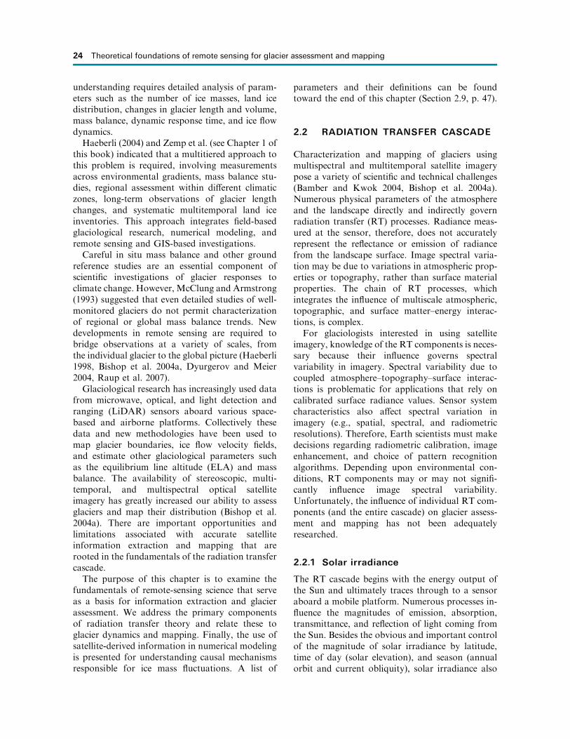
where A� is the area of the solar disk and des is theEarth–Sun distance which is a function of time.Variations in measured exoatmospheric spectralirradiance are caused by solar atmospheric interac-tions, and this can be compared with the blackbodyapproximation (Fig. 2.1). Standard exoatmosphericirradiance spectra can be used for the computationof spectral band irradiance values needed for theradiometric calibration of imagery.

2.2.2 Surface irradiance

Radiation is transmitted through the atmosphere,and atmospheric constituents and topographic fac-tors dictate the magnitude of radiation that reachesthe surface. Surface irradiance (E) is a composite ofthree downward irradiance components that arewavelength (�) dependent such that

Eð�Þ ¼ Ebð�Þ þ Edð�Þ þ Etð�Þ; ð2:3Þwhere Eb is direct beam irradiance, Ed is diffuseskylight irradiance (Ed), and Et represents adjacentterrain irradiance. Individually and collectivelythese irradiance components govern a variety ofsurface processes such as ablation, and also dictatethe magnitude of surface reflectance and emission.Depending upon environmental conditions, thesecomponents have varying degrees of influence onimage spectral variability.

2.2.2.1 Direct solar spectral irradiance

Under cloudless skies the direct irradiance com-ponent constitutes the dominant term in equation(2.3). Much research has been conducted to modelatmospheric transmittance functions accurately.The atmosphere attenuates direct irradiance pri-marily by gaseous absorption and molecular andaerosol scattering (Chavez 1996). These atmo-spheric processes are wavelength dependent andspatially and temporally controlled by changingatmospheric and landscape conditions. Total down-ward atmospheric transmission (T#) is a function of

Radiation transfer cascade 25

Figure 2.1. Comparison of exoatmospheric spectral

irradiance from the composite SMARTS2 spectrum

and a blackbody approximation. The SMARTS2 spec-

trum is a composite spectrum based in part on the

WRC85 spectrum and balloon and satellite observa-

tions (after Gueymard 1995).

the total optical depth of the atmosphere whichvaries with solar zenith angle and altitude, andcan be represented as

T#ð�Þ ¼ Trð�ÞTað�ÞTO3ð�ÞTgasð�ÞTH2O

ð�Þ; ð2:4Þwhere Tr is Rayleigh transmittance, Ta is aerosoltransmittance, TO3

is ozone transmittance, Tgas istransmittance for miscellaneous well-mixed gases,and TH2O

is water vapor transmittance. Atmo-spheric attenuation is highly variable withwavelength, with Rayleigh and aerosol scatteringdominating at shorter wavelengths and water vaporabsorption at longer wavelengths (Fig. 2.2). Directirradiance into the surface is also governed bymultiscale topographic effects. Local or microscaletopographic variation is represented by the inci-dence angle of illumination (i) between the incom-ing beam and the vector normal to the ground, suchthat

cos i ¼ cos �i cos �t þ sin �i sin �t cos ð�t � �iÞ; ð2:5Þwhere �i is the incident solar zenith angle, �i is theincident solar azimuth angle, �t is the slope angle ofthe terrain, and �t is the slope–aspect angle of theterrain.

Estimation of i is possible with the use of a digitalelevation model (DEM), and uncertainty in theestimate is related to the measurement scale, assubpixel-scale topographic variation is notaccounted for. Values of cos i can be �0:0, indi-cating no direct irradiance due to the orientation ofthe topography. It is important to note that the

incident solar geometry varies across the landscape,although this is usually assumed to be constantwhen working with individual image scenes (i.e.,small-angle approximation). In addition, mesoscaletopographic relief in the direction of �i determinesif a pixel is in shadow (S). This parameter value willbe 0:0 or 1:0 depending upon the presence orabsence of a cast shadow, respectively. Satelliteimagery acquired in rugged terrain or with rela-tively large solar zenith angles will exhibit castshadows. This can be accounted for by ray tracing,shadow detection, and shadow interpolation algo-rithms that alter cos i values appropriately (Dozieret al. 1981, Rossi et al. 1994, Giles 2001). Localtopography and shadows cast increase the globalspectral variance in satellite images, with a decreasein spectral variance within shadowed areas. Collec-tively, the aforementioned parameters define thedirect irradiance component as

Ebð�Þ ¼ E0ð�ÞT#ð�Þ cos iS: ð2:6Þ

In high-latitude and mountainous environments,this irradiance component can have a significantinfluence on glacier dynamics and image spectralvariability. Local topographic variations in param-eters such as slope magnitude and azimuth lead tosignificant variation in Eb due to ablation, supra-glacial fluvial action, and supraglacial debris trans-port processes. Furthermore, spatial variations inslope occur as a function of altitude (Fig. 2.3).Finally, the glacier altitude range determines the


Figure 2.2. Simulated atmospheric transmittance in the shortwave spectrum at the terminus of the Baltoro Glacier

near K2 in Pakistan on August 14, 2004 at 10:00 AM. Latitude: 35.692243� N; longitude: 76.165222� E; altitude:

3,505 m; solar zenith angle: 36.19�; precipitable water: 1.0 cm; ozone: 0.35 cm.

relative influence of atmospheric transmittance onthis component.

In general, this component is significant andhighly variable across most mountain landscapesexhibiting moderate to extreme relief (Fig. 2.4).Such variability is present in satellite imagery andusually needs to be accounted for using topographicnormalization techniques. Unfortunately, manymethods of topographic normalization do noteffectively remove this component from satelliteimagery, as they do not inherently account formultiscale topographic effects. Automated algo-rithms for thematic mapping are sensitive to suchspectral variations caused by Eb and can classifysteep slopes, cast shadows, moisture-laden debris,and surface water as the same feature. Conse-quently, classification accuracy can be highly vari-able depending upon the extent of topographicvariability. Empirical spectral feature extraction(e.g., image ratioing and principal componentanalysis) techniques are frequently used to reducethese topographic effects, although they can stillinfluence classification results depending upon whatapproach or algorithm is used.

2.2.2.2 Diffuse skylight spectral irradiance

Atmospheric scattering generates a hemisphericalsource of irradiance. This source can be simplis-

tically represented as a composite including aRayleigh-scattered component (Er), an aerosol-scattered component (Ea), and a ground-backscattered component (Eg) that represents inter-reflections between the landscape surface and theatmosphere, where

Edð�Þ ¼ Erð�Þ þ Eað�Þ þ Egð�Þ: ð2:7ÞIts accurate estimation is complicated by the factthat an anisotropic parameterization scheme isrequired. In general, diffuse skylight irradiancedecreases with angular distance from the Sun. Inaddition, this irradiance component is also influ-enced by mesoscale hemispherical shielding of thetopography. Consequently, only a solid angle of thesky will contribute to Ed , and this angle will changeas a function of pixel location and azimuth. Ingeneral, the solid angle will increase with altitude.It is frequently referred to as the sky view factor(Vf ) in the remote-sensing and energy balanceliterature, and can be estimated using a DEM suchthat

Vf ¼X2��¼0

cos2 �maxð�; dÞ��

2�; ð2:8Þ

where �max is the maximum local horizon angle ata given azimuth, �, over a radial distance of d. Inmountain environments exhibiting extreme relief


Figure 2.3. Slope–altitude plots for four alpine glaciers in the Karakoram Himalaya. Geomorphometric analysis

was conducted using a SRTM 90m digital elevation model. Average slope values were computed over a 50m

altitude interval. Different magnitudes and altitude trends are depicted. Such variation increases when a smaller

altitude interval is used.

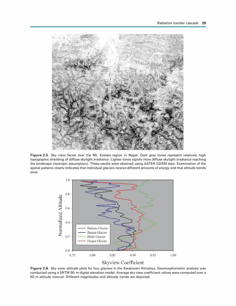
(deep valleys), topographic shielding of skylightdiffuse irradiance can be significant (Proy et al.1989). Consequently, the sky view factor is impor-tant in environments where climate variability andglacier erosion can generate moderate to extremetopographic relief (Fig. 2.5). It will be relativelyinsignificant in environments with minimal topo-

graphic relief. Where significant, individual glacierswithin a region receive variable amounts of energyfrom this component. Glacier fluctuations and massmovements alter the relief and ridgelines, such thatglacier surfaces exhibit sky view variations withaltitude (Fig. 2.6). Furthermore, difficulties inaccu-rately predicting the bidirectional reflectance distri-


Figure 2.4. Simulations of local and mesoscale topographic influences on direct irradiance for the Mt. Everest

region in Nepal. Grayscale values represent the collective magnitude of cos iS that is proportional to Ebwithout the

influence of the atmosphere. Simulation results were obtained using ASTER GDEM data and different solar

geometry. A. Solar zenith and azimuth angles of 0 and 135�, respectively. B. Solar zenith and azimuth angles

of 45 and 135�, respectively. C. Solar zenith and azimuth angles of 70 and 135�, respectively. D. Solar zenith and

azimuth angles of 85 and 135�, respectively.

A B

C D


Figure 2.5. Sky view factor over the Mt. Everest region in Nepal. Dark gray tones represent relatively high

topographic shielding of diffuse skylight irradiance. Lighter tones signify more diffuse skylight irradiance reaching

the landscape (isotropic assumption). These results were obtained using ASTER GDEM data. Examination of the

spatial patterns clearly indicates that individual glaciers receive different amounts of energy and that altitude trends

exist.

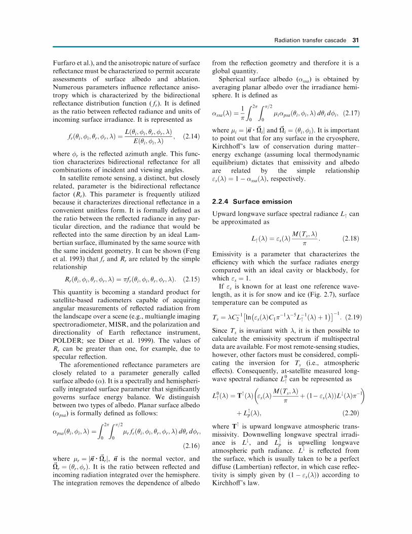
Figure 2.6. Sky view–altitude plots for four glaciers in the Karakoram Himalaya. Geomorphometric analysis was

conducted using a SRTM 90 m digital elevation model. Average sky view coefficient values were computed over a

50 m altitude interval. Different magnitudes and altitude trends are depicted.

bution function (BRDF) of land cover adjacent to aparticular location generates uncertainty in the esti-mation of the ground-backscattered component.

Such mesoscale land cover and topographiceffects on this irradiance component are presentin satellite imagery, although visual detection isdifficult due to the dominance of direct irradianceand surface reflectance. In addition, lower spatialfrequency components are difficult to detect andreduce, as topographic normalization approachesdo not effectively address this irradiance com-ponent.

More research is required to determine what themagnitude of this topographic effect is on imagespectral variability. However, the magnitude canbe deemed as potentially crucial in certain limitedbut important cases. The diffuse skylight irradiancecomponent generally is of the order of 5–10% ofdirect irradiance, as any photographer knows, or asgauged from the ASTER VNIR-band DN values intypical mountain shadows compared with directlyilluminated terrain. In heavily shadowed zones(such as in northern-aspect cirque glaciers in theNorthern Hemisphere), the diffuse skylight com-ponent can approach the direct solar beam in itsimportance to the energy budget. The sky viewfactor in rough terrain, such as in Himalayan val-leys, can then account for blocking up to half, oreven more, of the diffuse skylight. In general, rela-tive to direct beam irradiance, diffuse skylight andskyview shielding each become more important asrelief increases (e.g., in narrow canyons) and aslatitude increases (MacClune et al. 2003).

2.2.2.3 Adjacent terrain spectral irradiance

The irradiance components Eb and Ed interact withthe terrain and land cover biophysical characteris-tics to generate an adjacent terrain irradiance com-ponent (Et).

This irradiance component is not generally con-sidered in remote-sensing and energy balancestudies because it is assumed that its magnitude isrelatively minor and it is a difficult parameter toestimate accurately. A first-order approximationwas formulated by Proy et al. (1989) and assumesthat reflected surface radiance is Lambertian. It isthen possible to estimate the radiance received atany pixel by accounting for the geometry betweentwo pixels ( p1 and p2) such that

L12 ¼ cos �1 L2 cos �2Ap

d2

� �� ; ð2:9Þ

where L12 represents the radiance received at p1from the luminance of p2 (L2), �1 and �2 are theangles between the normal to the terrain and thedirect line of sight from p1 to p2, Ap is the pixel area( p2), and d represents the distance between p1 andp2.This equation can be used to estimate Et for any

pixel by integrating over all of the pixels whoseslopes are oriented towards a pixel of interest andwhere the line of sight is not blocked by the topog-raphy. High-altitude and extreme local relief areascan exhibit a strong adjacent terrain irradiancecomponent due to highly reflective features suchas snow and vegetation.

2.2.3 Surface reflectance

The magnitude of reflected and emitted radiance atthe surface is determined by the conservation ofenergy, and is expressed by Kirchhoff’s law as

�ð�Þ þ �að�Þ þ Tð�Þ ¼ 1:0; ð2:10Þwhere, �, �a, and T represent reflectance, absorp-tion, and transmission, respectively. For opaqueobjects T ¼ 0:0. Therefore, spectral reflectancecan be approximated as

�ð�Þ ¼ MðTs; �ÞEð�Þ ; ð2:11Þ

where Ts is surface temperature. Given a Lamber-tian surface, which reflects radiation equally in alldirections, reflected surface spectral radiance (L)can be computed as follows:

Lð�Þ ¼ �ð�Þ Eð�Þ�

� �: ð2:12Þ

Satellite imagery can be used to estimate surfaceradiance and reflectance, although atmosphericcorrection is required. In general, this can beapproximated as

Lð�Þ ¼ ðL0ð�Þ � Lpð�ÞÞ=T"ð�r; �Þ; ð2:13Þwhere L0 is at-satellite measured radiance, Lp isadditive path radiance from the atmosphere, andT" is upward total atmospheric transmittance thatis a function of the reflected zenith angle (�r) andwavelength.

2.2.3.1 Bidirectional reflectance distributionfunction and albedo

Unfortunately, the Lambertian assumption is notvalid on glaciers (see Chapter 3 of this book by


Furfaro et al.), and the anisotropic nature of surfacereflectance must be characterized to permit accurateassessments of surface albedo and ablation.Numerous parameters influence reflectance aniso-tropy which is characterized by the bidirectionalreflectance distribution function ( fr). It is definedas the ratio between reflected radiance and units ofincoming surface irradiance. It is represented as

frð�i; �i; �r; �r; �Þ ¼Lð�i; �i; �r; �r; �Þ

Eð�i; �i; �Þ; ð2:14Þ

where �r is the reflected azimuth angle. This func-tion characterizes bidirectional reflectance for allcombinations of incident and viewing angles.

In satellite remote sensing, a distinct, but closelyrelated, parameter is the bidirectional reflectancefactor (Rr). This parameter is frequently utilizedbecause it characterizes directional reflectance in aconvenient unitless form. It is formally defined asthe ratio between the reflected radiance in any par-ticular direction, and the radiance that would bereflected into the same direction by an ideal Lam-bertian surface, illuminated by the same source withthe same incident geometry. It can be shown (Fenget al. 1993) that fr and Rr are related by the simplerelationship

Rrð�i; �i; �r; �r; �Þ ¼ �frð�i; �i; �r; �r; �Þ: ð2:15ÞThis quantity is becoming a standard product forsatellite-based radiometers capable of acquiringangular measurements of reflected radiation fromthe landscape over a scene (e.g., multiangle imagingspectroradiometer, MISR, and the polarization anddirectionality of Earth reflectance instrument,POLDER; see Diner et al. 1999). The values ofRr can be greater than one, for example, due tospecular reflection.

The aforementioned reflectance parameters areclosely related to a parameter generally calledsurface albedo (�). It is a spectrally and hemispheri-cally integrated surface parameter that significantlygoverns surface energy balance. We distinguishbetween two types of albedo. Planar surface albedo(�psa) is formally defined as follows:

�psað�i; �i; �Þ ¼Z 2�

0

Z �=2

0

�r frð�i; �i; �r; �r; �Þ d�r d�r;

ð2:16Þwhere �r ¼ j~nn E~��rj, ~nn is the normal vector, and~��r ¼ ð�r; �rÞ. It is the ratio between reflected andincoming radiation integrated over the hemisphere.The integration removes the dependence of albedo

from the reflection geometry and therefore it is aglobal quantity.Spherical surface albedo (�ssa) is obtained by

averaging planar albedo over the irradiance hemi-sphere. It is defined as

�ssað�Þ ¼1

�

Z 2�

0

Z �=2

0

�i�psað�i; �i; �Þ d�i d�i; ð2:17Þ

where �i ¼ j~nn E~��ij and ~��i ¼ ð�i; �iÞ. It is importantto point out that for any surface in the cryosphere,Kirchhoff’s law of conservation during matter–energy exchange (assuming local thermodynamicequilibrium) dictates that emissivity and albedoare related by the simple relationship"sð�Þ ¼ 1� �ssað�Þ, respectively.

2.2.4 Surface emission

Upward longwave surface spectral radiance L" canbe approximated as

L"ð�Þ ¼ "sð�ÞMðTs; �Þ

�: ð2:18Þ

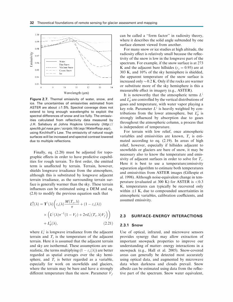
Emissivity is a parameter that characterizes theefficiency with which the surface radiates energycompared with an ideal cavity or blackbody, forwhich "s ¼ 1.If "s is known for at least one reference wave-

length, as it is for snow and ice (Fig. 2.7), surfacetemperature can be computed as

Ts ¼ �C�12 ln "sð�ÞC1�

�1��5L�1" ð�Þ þ 1

� � ��1: ð2:19Þ

Since Ts is invariant with �, it is then possible tocalculate the emissivity spectrum if multispectraldata are available. For most remote-sensing studies,however, other factors must be considered, compli-cating the inversion for Ts (i.e., atmosphericeffects). Consequently, at-satellite measured long-wave spectral radiance L0

" can be represented as

L0"ð�Þ ¼ T"ð�Þ "sð�Þ

MðTs; �Þ�

þ ð1� "sð�ÞÞL#ð�Þ��1

� �

þ L"pð�Þ; ð2:20Þ

where T" is upward longwave atmospheric trans-missivity. Downwelling longwave spectral irradi-ance is L#, and L"

p is upwelling longwaveatmospheric path radiance. L# is reflected fromthe surface, which is usually taken to be a perfectdiffuse (Lambertian) reflector, in which case reflec-tivity is simply given by (1� "sð�Þ) according toKirchhoff’s law.


Finally, eq. (2.20) must be adjusted for topo-graphic effects in order to have predictive capabil-ities for rough terrain. To first order, the emittedterm is unaffected by terrain. Terrain, however,shields longwave irradiance from the atmosphere,although this is substituted by longwave adjacentterrain irradiance, as the surrounding terrain sur-face is generally warmer than the sky. These terraininfluences can be estimated using a DEM and eq.(2.8) to modify the previous equation such that

L0"ð�Þ ¼ T"ð�Þ

�"sð�Þ

MðTs; �Þ�

þ ð1� "sð�ÞÞ

� L#ð�Þ��1ð1� Vf Þ þ 2�L#t ðTt; �ÞVf

��

þ L"pð�Þ; ð2:21Þ

where L#t is longwave irradiance from the adjacent

terrain and Tt is the temperature of the adjacentterrain. Here it is assumed that the adjacent terrainand sky are isothermal. These assumptions are un-realistic, the terms multiplying (1� "sð�Þ) are betterregarded as spatial averages over the sky hemi-sphere, and Tt is better regarded as a variable,especially for work on snowfields and glaciers,where the terrain may be bare and have a stronglydifferent temperature than the snow. Parameter Vf

can be called a ‘‘form factor’’ in radiosity theory,where it describes the solid angle subtended by onesurface element viewed from another.For many snow or ice studies at high altitude, the

radiosity effect is relatively small because the reflec-tivity of the snow is low in the longwave part of thespectrum. For example, if the snow surface is at 273K and the adjacent bare hillsides ("s ¼ 0:95) are at303 K, and 10% of the sky hemisphere is shielded,the apparent temperature of the snow surface isincreased only�0:2 K. Only if the rocks are warmeror substitute more of the sky hemisphere is this ameasurable effect in imagery (e.g., ASTER).It is noteworthy that the atmospheric terms L#

and L"p are controlled by the vertical distributions of

gases and temperature, with water vapor playing akey role. Parameter L# is heavily weighted by con-tributions from the lower atmosphere, but L"

p isstrongly influenced by absorption due to gasesthroughout the atmospheric column, a process thatis independent of temperature.For terrain with low relief, once atmospheric

variables and emissivities are known, Ts is esti-mated according to eq. (2.19). In areas of highrelief, however, especially if hillsides adjacent tosnowfields or glaciers are bare of snow, it may benecessary also to know the temperature and emis-sivity of adjacent surfaces in order to solve for Ts.Here it is best to use a temperature/emissivityseparation algorithm to estimate both temperaturesand emissivities from ASTER images (Gillespie etal. 1998). Although noise-equivalent change in tem-perature (evaluated at 300 K) for ASTER is <0:3K, temperatures can typically be recovered onlywithin �1 K, due to compounded uncertainties inatmospheric variables, calibration coefficients, andassumed emissivity.

2.3 SURFACE–ENERGY INTERACTIONS

2.3.1 Snow

Use of optical, infrared, and microwave sensorsprovides synergy that may allow extraction ofimportant snowpack properties to improve ourunderstanding of matter- energy interactions in asnowpack (e.g., Hall et al. 2005). Snow-coveredareas can generally be detected most accuratelyusing optical data, and augmented by microwavedata when darkness and clouds prevail. Snowalbedo can be estimated using data from the reflec-tive part of the spectrum. Snow water equivalent,


Figure 2.7. Thermal emissivity of water, snow, and

ice. The uncertainties of emissivities estimated from

ASTER are about �1:5%. Spectral coverage does not

extend to long enough wavelengths to exploit the

spectral differences of snow and ice fully. The emissiv-

ities calculated from reflectivity data measured by

J.H. Salisbury at Johns Hopkins University (http://

speclib.jpl.nasa.gov/scripts/lib/asp/WaterResp.asp),

using Kirchhoff’s Law. The emissivity of natural rough

surfaces will be increased and spectral contrast lowered

due to multiple reflections.

however, is an important hydrologic parameter,and can be estimated using microwave wavelengthsthat penetrate the snowpack or emanate from theground.

One of the first observations made in the study ofearly satellite images of the Earth’s surface wascoverage of some surfaces by high-albedo snow.Surface albedo is the ratio of upwelling reflectedflux to downwelling incident irradiance. New,fine-grained snow cover reflects more than �80%of incident solar radiation, while older, coarse-grained and/or melted and refrozen snow tends toreflect far less radiation (Fig. 2.8), especially when ithas been covered by soot/dust or volcanic ash.Broadband albedo is reflectance across the reflectivepart of the solar spectrum. Broadband albedodecreases when grain size increases as the snow ages(Choudhury and Chang 1979), and melting causessnow grains to grow and bond into clusters (Dozieret al. 1981, Warren 1982, Dozier 1989).

With the onset of surface melting and associatedgrain size increases, near-infrared reflectancedecreases dramatically (e.g., Fig. 2.8; Warren andWiscombe 1980, Warren 1982). The near-infraredalbedo of snow is very sensitive to snow grain sizewhile visible albedo is less sensitive to grain size, butis affected by snow impurities. For example, for thecase of just 3 ppm of soot in snow, see the computedspectra in Figure 3.6 (Furfaro et al.’s chapter), andcompare also with their computed Figure 3.4 for

pure snow and our Figure 2.8 for actual snow.Warren and Wiscombe (1980) considered the casefor snow containing aerosol impurities. Effectivesnow grain radii typically range in size from�50 mm for new snow, to 1mm for wet snow con-sisting of clusters of ice grains (Warren 1982). Snowalbedo may decrease by >25% within just a fewdays as grain growth occurs (Nolin and Liang2000). The albedo of a snow cover, if it is thin, isalso influenced by the albedo of the land, especiallywhen vegetation extends above the snow surface.Snow albedo can be approximated over large

areas by deriving the linear relationship betweenthe brightest snow-covered areas such as arctic tun-dra and the darkest snow-covered forest in a scene.Albedos can be assigned 0:80 and 0:18, respectively,as did Robinson and Kukla (1985) using DefenseMeteorological Satellite Program (DMSP) imagery(0.4–1.1 mm). Linear interpolation was then per-formed to derive albedo. Today, snow albedo canbe estimated directly from satellite data using theModerate-resolution Imaging Spectroradiometer(MODIS) (e.g., Klein and Stroeve 2002, Schaaf etal. 2002).A near-surface global algorithm has been devel-

oped to map snow albedo using MODIS data. Inderiving albedo, atmospherically corrected MODISsurface reflectance in individual MODIS bands forsnow-covered pixels located in nonforested areasis adjusted for anisotropic scattering effects usinga discrete ordinates radiative transfer model(DISORT) and snow optical properties (Kleinand Stroeve 2002). Currently in the algorithm,snow-covered forests are considered to be Lamber-tian reflectors. The adjusted spectral albedos arethen combined into a broadband albedo measure-ment using a narrow-to-broadband conversionscheme developed specifically for snow (Nolinand Liang 2000, Klein and Stroeve 2002). Thusderived, a near-global snow albedo product isavailable as part of the suite of MODIS snow coverproducts and has been since February 2000 (Halland Riggs 2007).In the thermal region, eq. (2.21) is underdeter-

mined, and a solution for Ts requires independentinformation, especially for atmospheric conditions.For ASTER images, these data have come fromNCAR/CIRES reanalysis data from radiosondeprobes of water, temperature, and pressure profiles.These profiles are converted to L# and L"

p using theMODTRAN radiative transfer model. For work onsnow and ice, emissivity is generally measured in thelaboratory or taken from a spectral library. For

Surface–energy interactions 33

Figure 2.8. Reflectance of snow with different effec-

tive particle size. Reflectivity data obtained from the

ASTER Spectral Library (http://speclib.jpl.nasa.gov),

which was collected at the Johns Hopkins University

IR Spectroscopy Lab. The laboratory spectra here may

be compared with idealized radiative transfer–based

computed spectra of pure ice shown in Figure 3.4 of

this book (Furfaro et al.’s chapter).

snow and ice, terrain irradiance is less important inthe thermal infrared than in the visible, near-infra-red, and shortwave infrared, because snow and icehave reflectivities <5% between wavelengths of 8and 12 mm (Fig. 2.7). Nevertheless, steep, bare rockwalls above glaciers will have a measurable effect,all the more important because the reflectivity ofsnow and ice differ at longer wavelengths, withsnow a factor of two or more less reflective thanice. Estimation of snow and ice temperatures is bestmade at �10:5 mm, because the emissivities areabout the same and no distinction between themis necessary in advance.

2.3.2 Glaciers

Glacier surfaces are composed of a variety ofmaterials that exhibit unique reflectance patterns.High spatial variability in reflectance results fromvariations in the debris cover, ice properties, surfacemoisture content, and snow and firn properties. Forexample, in ablation areas, debris cover lithology,depth, and surface roughness significantly affectablation and moisture content, while reflectancefrom ice surfaces is dominated by properties suchas air bubble and englacial load characteristics.Furthermore, centimeter-scale roughness fromcryoconite holes in ice can produce additional spec-tral reflectance variation. In the accumulation area,reflectance is controlled by the magnitude of meta-morphism of ice crystals, firm density, and moisturecontent (Rees 2006). Collectively, surface matterand property variation, multiscale topographiceffects, and variations in solar geometry result inanisotropic reflectance (Greuell and de Wildt 1999).

Greuell and de Wildt (1999) measured andempirically modeled the anisotropic reflection ofthe radiation of melting glacier ice on theMorteratschgletcher Glacier in Switzerland. Theyfound that anisotropy increases with longer wave-lengths (Fig. 2.9), with increasing �i, and withdecreasing �. Wavelength dependence can beexplained due to changes in the absorption coeffi-cient of ice with wavelength (Grenfell and Perovich1981). A higher absorption coefficient produceslower surface albedo, which also dictates the shortereffective pathlength of photons through the ice.Statistically, a shorter pathlength governs thenumber of scattering events, which leads to betterpreservation of the angular distribution of photonsin multiple scattering events, which is described bythe scattering phase function fp. The amount ofanisotropy increases with decreasing �i for snow-covered glaciers, as forward-scattered photonspenetrate more deeply for small zenith angles,and photons are more evenly distributed (Warrenet al. 1998). Lower albedo is caused by surfaceimpurities and debris that can sometimes increasesurface meltwater, which subsequently affects theabsorption coefficient in a positive feedback.The relationships between fundamental radio-

metric parameters and various properties of theglacier surface can be made explicit by consideringthe basic physical laws that describe the conserva-tion of energy for photons being transported acrossparticulate media. As photons reach the glaciersurface they enter the ice–snow–firn medium andare subject, in principle, to the same absorption-scattering mechanisms that occur in the atmo-sphere. Nevertheless, glacier surface properties are


Figure 2.9. Broadband BRDFs measured over melting glacier ice: (left) Thematic Mapper band 2, �i ¼ 50�,� ¼ 0:52; (right) Thematic Mapper band 4, �i ¼ 50�, � ¼ 0:50 (modified after Greuell and de Wildt 1999).

very different than atmospheric properties. Usingfirst principles, physical models can be derived tocompute the spectral radiance leaving the glaciersurface, as well as to compute the BRDF/BRFparameters to provide knowledge of surface behav-ior. In the specific case of glaciers, the theoreticalcomputation of the BRDF/BRF is generallyaccomplished by assuming the surface to be ahomogeneous, plane-parallel particulate layer ofice or snow, and solving the corresponding radia-tion transfer equation (RTE). If the optical proper-ties (scattering and absorption coefficient and fp) ofice or snow are known, the conservation of photonsin the appropriate phase space yields the linearizedBoltzmann equation such that

�@

@Lð; �; �Þ þ Lð; �; �Þ

¼ !

2

Z 1

�1

Z 2�

0

fpðcos�ÞLð; �0; �0Þ d�0 d�0: ð2:22Þ

Here we assume that radiance is a function of onlyone spatial dimension (depth) as well as a functionof inclination (� ¼ cos �i) and azimuthal angle (�i).Optical thickness () is related to thickness (h) viathe extinction coefficient ext( ¼ R h

0 extðhÞ dh).Single-scattering albedo, !, is the ratio betweenscattering and extinction, while fp describes theprobability that a photon moving in direction ~��0

is scattered in the direction ~��. Moreover, fp dependson� ¼ ~��0 E~�� (i.e., the angle between incoming andscattered photons).

Eq. (2.22) must be equipped with appropriateboundary conditions and solved numerically tocompute L. Various numerical techniques areavailable to solve the RTE and include the iterativesolution of the Ambartsumiam’s integral equation(Mishchenko et al. 1999), adding–doubling tech-nique (Hansen and Travis 1974), converged discreteordinates method (Ganapol and Furfaro, 2008),and analytical discrete ordinates method (Siewert2000). Areal and intimate mixtures of snow, ice,and debris can be modeled using radiative transfertheory (see Chapter 3).

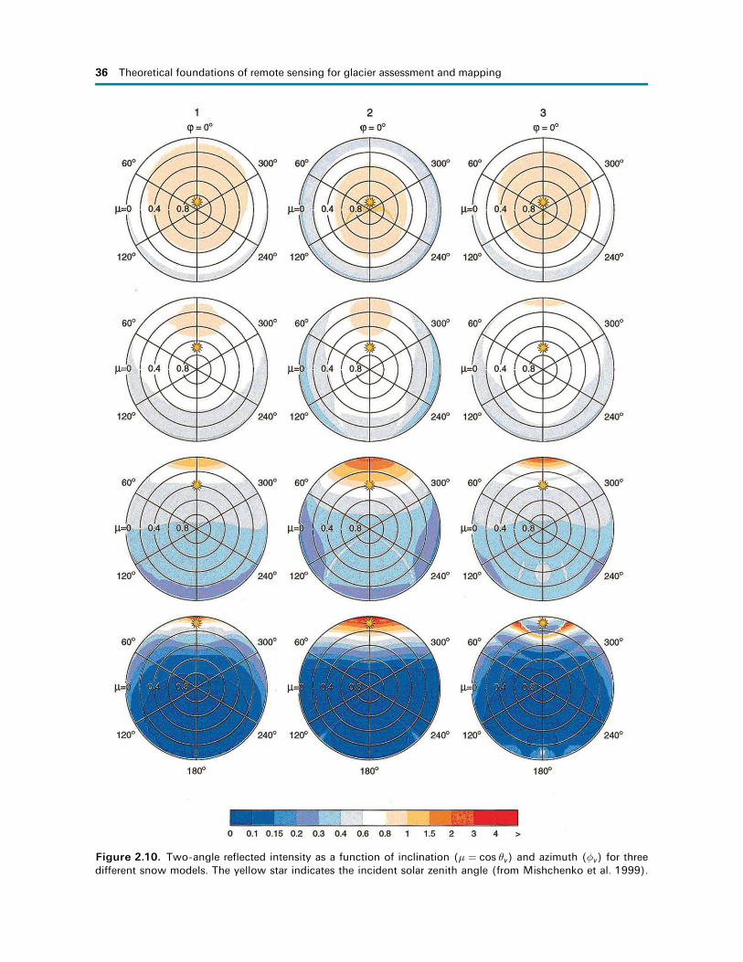
The computed radiance can be directly used toevaluate the theoretical BRDF and/or BRF fordifferent types of glaciers. Such parameters can beemployed to study the effect of particle size, shape,and orientation of ice crystals on the reflected sig-nal. Examples of a RT-computed BRF for ice par-ticle models are shown in Fig. 2.10. Mishchenko etal. (1999) considered three ice models including:(1) particles with a highly irregular, random fractal

shape (i.e., snow), (2) homogeneous ice spheres, and(3) regular hexagonal ice crystals. Reflected inten-sities are displayed in polar plots: each columncorresponds to an ice model (1, 2, and 3); the rowsshow BRF as a function of incident angle (the starson the plots indicate the inclination of the incidentphoton beam). Clearly, the scattering phase func-tion for the particle type has a marked effect on theBRF. While small differences are perceived whenlooking at the nadir direction across models, largevariations exist in other directions. Note that formodel 1, the BRF has less structure/features thanmodel 3 (i.e., degree of anisotropy). Indeed, a reg-ular hexagonal ice model has a more structuredphase function than a randomly oriented, fractal-like model.

2.3.3 Water

Increases in temperature and high ablation producesignificant quantities of meltwater that eventuallycan form supraglacial and proglacial lakes. Thereader is directed to the following chapter by Fur-faro et al. for further theoretical treatment of thistopic of radiative transfer in glacial waters. Theinteraction between light and water is dictated bythe same first principles describing photon propaga-tion in particulate media. The physics of interactionare described by eq. (2.22) which formalizes theconservation of photons either absorbed or scat-tered or eventually reemitted in any direction.Naturally, there are key differences and similaritiesthat markedly distinguish the transport of light inwater from any other medium. For example, in thecase of water–light interaction, the visible part ofthe spectrum, 400–700 nm, is of interest because it isrelated to biological activity, and is the regionwhere optical transmission is the largest. From amodeling point of view, glacier meltwater lakes canbe modeled using the so-called plane-parallelapproximation. Here it is generally assumed thatthe water column is layered and incident radiationis uniform over the surface.Optical properties play a critical role in determin-

ing the behavior of reflected light as collected byobserving sensors. Such properties (i.e., absorption,refraction, and scattering) are generally difficult tocharacterize. Water is the primary compound thatalso potentially incorporates organic and inorganicmatter. These constituents exhibit high spatio-temporal variability in concentration. Multiplecomponents are generally present within the water,and it is assumed that the absorption and scattering

Surface–energy interactions 35


Figure 2.10. Two-angle reflected intensity as a function of inclination (� ¼ cos �v) and azimuth (�v) for three

different snow models. The yellow star indicates the incident solar zenith angle (from Mishchenko et al. 1999).

coefficients of individual, optically active constitu-ents are additive. We can distinguish between clearwater and turbid meltwater. For water, opticalproperties are primarily determined by the concen-tration of suspended detritus. Indeed, there is aformal correlation between absorption (ap) andscattering (bp) coefficients and concentration of par-ticles (C) which can be described as follows (Prieurand Sathyendranath 1981):

apð�Þ ¼ 0:06A0pð�ÞC0:602; ð2:23Þ

bpð�Þ ¼ 0:5B0pð�Þ

550

�

� �C0:62: ð2:24Þ

A0p and B0

p range between 0.12 and 0.45 m�1. Forturbid water, the optical properties (including spec-tral variation in reflectance) are strongly influencedby mineral particle concentration. Suspended sedi-ments/particles tend to be scatterers rather thanabsorbers. Nevertheless, the mineralogical compo-sition of the particles can also be a factor especiallyin the case of iron-rich sediments that feature strongabsorption bands.

Turbid glacier meltwaters exhibit an extremelyforward-peaked scattering, with a peak forwardto backscatter ratio on the order of 106. Scatteringhas been modeled using a forward-peaked phasefunction derived by experimental data (Petzold1972) and analytical models such as theFournier–Fourand model (Fournier and Fourand1994).

2.4 COMPLICATIONS

The previous sections outline the complexity ofradiation transfer and the relatively large numberof variables that influence sensor spectral response.Information extraction from satellite data is predi-cated upon isolating specific variance componentsof the radiation transfer cascade. This frequentlyrequires radiometric calibration to account for thesignificant variables that cause spectral variation. Inpractice, accurate information necessary to utilizingphysical models to reduce unwanted variationcaused by the atmosphere or the topography isnot readily available, and Earth scientists typicallyrely upon empirical approaches to reduce or isolatespectral variation.

A classic example for glacier assessment includestopographic normalization of satellite imagery.Glaciologists rarely account for all the irradiancecomponents and viewing geometry related to

topography. Instead, empirical procedures such asratioing or principal component analysis is used toreduce topographic effects. This is usually effectivefor thematic mapping applications, although quan-titative estimation of surface parameters requiresmore detailed insight and treatment of the radiationtransfer cascade.

2.5 SPACE-BASED INFORMATION

EXTRACTION

Satellite imagery contains a wealth of informationfor assessing the Earth’s cryosphere (Bishop et al.2004a). Extracting these signals and pertinentglacier information can be challenging. New tech-niques and analytical approaches are frequentlyrequired to identify and transform spectral varia-tion into thematic and quantitative parameters. Wefocus here on the type of information that can beextracted from satellite imagery.

2.5.1 Snow cover

Snow cover mapping can be accomplished at avariety of temporal and spatial scales with highaccuracy. Today, satellite-borne instruments pro-vide detailed information on snow cover in thevisible, infrared, and microwave parts of the elec-tromagnetic spectrum on a daily basis at a globalscale. In 1997, the Interactive Multi-sensor Snowand Ice Mapping System (IMS) began to produceoperational products daily at a spatial resolution ofabout 25 km, utilizing a variety of satellite data(Ramsay 1998). Improvements in the spatial reso-lution of the IMS product in February 2004 resultedin snow maps at 4 km resolution. In June 1999,NOAA/NESDIS ceased producing weekly maps,replacing them with the daily IMS product (Ram-say 1998).Since February 24, 2000 the Moderate Resolu-

tion Imaging Spectroradiometer (MODIS) sensorhas been providing daily snow maps at a varietyof different temporal and spatial resolutions (Halland Riggs 2007). MODIS is a 36-channel imagingspectroradiometer that was first launched as part ofNASA’s Earth Observing System (EOS) programon December 18, 1999 on the Terra spacecraft. Asecond MODIS was launched on May 4, 2002 onthe Aqua spacecraft. Snow maps are available fromMODIS to serve the needs of local, regional, andglobal modelers and are provided at 500 m, 5 km,and 25 km resolution, and as daily, weekly, or

Space-based information extraction 37

monthly composites, including fractional snowcover and albedo (Hall and Riggs 2007). Snowcover maps are also routinely generated usinghigher resolution satellite imagery coupled with avariety of pattern recognition methods. This resultsfrom the good statistical separability between snowreflectance and the reflectance of other land-coverclasses.

2.5.2 Ice sheets

Using Advanced Very High Resolution Radiometer(AVHRR) data and, more recently, MODIS data, itis possible to achieve daily mapping of the Green-land Ice Sheet. With microwave data, most cloudcover is not an issue, but there are also many com-plexities in terms of what is being observed, and theuse of data from optical wavelengths provides awealth of information about ice sheet characteris-tics including surface temperature and albedo.

Comiso (2006) has shown, using monthlyAVHRR-derived, surface temperature maps, thatmuch of the Arctic has been undergoing a steadywarming since 1981, including a 1:19�C per decadeincrease over Greenland. More recently, Hall et al.(2006) provided improved temporal and spatialdetail using 5 km resolution MODIS surface tem-perature maps that show the temperature distribu-tion in the various facies of the ice sheet. The glacierfacies (Benson 1996) are delineated based on snowand ice characteristics, and subsequently changes ofthe facies boundaries over time can be correlatedwith ice sheet mass balance. For example, usingsurface temperature maps, an increase in the eleva-tion of the boundary between the percolation anddry-snow facies could be monitored over time toreveal associated temporal changes in ice sheet massbalance.

Satellite data (AVHRR) have also been used tomap changes in albedo over the Greenland IceSheet during the spring and summer months (Knapand Oerlemans 1996, Nolin and Stroeve 1997,Stroeve et al. 1997, Comiso 2006). Recently, Stroeveet al. (2006) have used MODIS data to analyze theaccuracy of daily albedo measurements fromMODIS of the Greenland ice sheet.

Surface albedo over the Greenland Ice Sheet hasalso been measured using data acquired by the EOSMultiangle Imaging Spectroradiometer (MISR)instrument. MISR images the surface using ninediscrete, fixed angle cameras, one nadir viewingand four viewing angles in forward and aftwarddirections along the spacecraft track. Compared

with in situ measurements at five different sites,the surface albedo derived from two different meth-ods using MISR data showed good agreement(Stroeve and Nolin 2002). Although the atmosphereis relatively thin over the ice sheet, atmosphericattenuation is significant in the visible and near-infrared wavelengths.

2.5.3 Alpine glacier mapping

Glaciers are known to be directly and indirectlysensitive to climate variations, and a top priorityof assessing climate change is to monitor andunderstand glacier fluctuations at a variety of scales(Haeberli et al. 1998, Bishop et al. 2004a, Kargel etal. 2005, Haeberli 2004), and to quantify the errors(Hall et al. 2003). This requires information onchanges in glacier distribution.The nature and uncertainty of information

extracted from satellite imagery is strongly relatedto sensor characteristics. Relatively high spatialresolution and good image geometric fidelity isrequired to resolve smaller alpine glaciers andglacier features. High spatial resolution also permitsspatial analysis of glacier surfaces, such that ice flowand structural characteristics can be assessed andmapped (e.g., Bishop et al. 1998). In addition, scenecoverage should be large enough to enable regionalanalysis.Spectral resolution controls spectral differentia-

tion of glacier surfaces from other landscape feat-ures. Glacier surface reflectance is governed by icestructures and the concentration of air bubbles(Winther 1993), variations in grain size of snow/firn(Kaab 2005b), surface water content (Konig et al.2001), and dust and/or supraglacial debris.In general, the near and shortwave infrared

regions of the spectrum are important for snowand ice mapping, and many different satellitesensors can be used to map alpine glaciers that haveminimal debris cover. Atmospheric conditions,however, such as cloud cover and aerosol influencescan affect spectral response. The anisotropic natureof surface reflectance is also an issue, as multiscaletopographic effects can significantly influence inter-pretation (Bishop et al. 2004a, b). Existing spectralbandwidth characteristics, however, make it diffi-cult to map debris-covered glaciers as spectral dif-ferentiation between rocks and sediment on and offglaciers is relatively poor (Bishop et al. 2001, 2004b,Paul et al. 2004). Other issues include radiometricresolution and sensor gain which can lead to sensor


saturation over snow and ice, and repeat coveragewhich affects change detection studies.

Alpine glacier mapping can be accomplishedusing a variety of methods, each with advantagesand disadvantages. The most common approachused worldwide is based on cursor tracking, whichis commonly known as on-screen manual digitiza-tion from a false-color composite (FCC), and/orspectrally enhanced imagery (i.e., ratios or principalcomponents). This approach takes advantage ofspectral variations of landscape features; it is laborintensive and fraught with difficulties, as results arenecessarily dependent upon geographic knowledgeand experience of the analyst. Glacier boundariescan easily be misinterpreted. Other techniques forglacier boundary delineation include the imageratio approach (e.g., Hall et al. 1989, Paul et al.2002), supervised and unsupervised classification(e.g., Gratton et al. 1990, Aniya et al. 1996), andthe use of artificial neural networks (e.g., Bishop etal. 1999). Most of these techniques require imagepreprocessing and work reasonably well for cleanice, but they tend to fail for debris-covered glaciers.Details regarding mapping glaciers using satellitespectral data are covered in Chapter 4.

Change detection studies have produced esti-mates of retreat rates and changing mass balancesfor alpine glaciers around the world. The crucialfactors for temporal analysis include selectingsuitable images, identifying change categories, andusing appropriate change detection algorithms (Luet al. 2004). Space-based glacier change detectionstudies include monitoring of variations in terminusposition (retreat, advance, and/or surge), down-wasting, snow line, debris cover, exposed glacialarea, supraglacial lake fluctuations, and mass bal-ance. Some of these parameters may be interrelated,such as glacier terminus position and mass balancechanges (Haeberli and Hoelzle 1995), and changesin supraglacial debris thickness and cover andglacier surface downwasting. Paul et al. (2004) indi-cated that many glaciers are currently downwastinginstead of retreating. It is important to note, how-ever, that methods to measure annual mass balanceare still being studied (Khalsa et al. 2004).

2.5.4 Debris-covered glaciers

Mapping debris-covered glaciers is notoriously dif-ficult (Williams et al. 1991, Bishop et al. 2001).Different approaches have been attempted, andthe use of topographic information in addition tomultispectral imagery is generally required. Paul et

al. (2004) developed an automated approach tomap debris-covered glaciers using slope and curva-ture derived from a DEM and neighborhood anal-ysis. Bishop et al. (2001) used a scale-dependentautomated object-oriented approach which classi-fies debris-covered glaciers and surface featuressuch as ice cliffs and moraines. These examplesdemonstrate the feasibility of automated mappingof debris-covered glaciers, although the results arehighly dependent upon the quality and resolution ofthe DEM, and on the sophistication of theapproach. Research indicates that integrated datafusion approaches can be well suited to effectivelymake use of spectral data and multiple forms oftopographic information. Details regarding DEMgeneration and geomorphometry are covered inChapter 5.Data on the supraglacial debris cover character-

istics of glaciers is sorely needed, as debris coverexerts a tremendous influence on the ablation pro-cess (Nakawo and Rana 1999). Previous researchindicates a complex relationship between debriscover thickness and ablation, where debris covercan either retard or enhance ablation rates depend-ing on the spatial variability in debris lithology andthickness (Loomis 1970, Mattson et al. 1993).Remote-sensing studies indicate that debris coverthickness can be highly variable (Bishop et al.1995), and field research indicates a general patternof greater debris depths towards the terminus andlateral edges of many alpine glaciers (e.g., Gardnerand Jones 1993). These patterns are caused by massmovement and ice flow dynamics that transportdebris to the terminus and edges via horizontaland vertical advection. Increases in surface ablationand glacier surface downwasting overtime, andsometimes increases in delivery of debris to theglacier by landslides and other mass movements,can result in increases in the percentage of debriscover. Conversely, acceleration of flow due topositive mass balance or surging sometimes canmove debris to terminal and lateral moraines andpartially clear away debris from much of the glaciersurface. Consequently, field or remote-sensingassessment of debris cover patterns and debrisdepth variability is essential for estimatingablation, glacier mass balance, glacier sensitivityto climate change, and water supply from the abla-tion area.Satellite imagery can be used to map variations in

supraglacial lithologies. For example, Nakawo etal. (1993) were able to differentiate and map areasof granitic and schistose debris over the Khumbu


Glacier in Nepal. In other areas in the Himalaya,the predominant debris lithologies can be mappedand include differentiation of: (1) granitic andblack metasediment debris in the Hindu Kush,(2) granodiorite, weathered granodiorite, and blackmetasediments in the Hunza Himalaya, and(3) granite, gneiss, and black and red metasedimentdebris in the Karakoram Himalaya. Such capabil-itites also exist for debris-covered glaciers in Alaskaand the AndesMountains. Difficulties in automatedmapping and lithologic characterization of debrisresult from spectral variation caused by glaciertopography, moisture-laden debris, and supra-glacial lakes. This is especially the case when debrislithology is predominately mafic in compositionand numerous features exhibit relatively low reflec-tance throughout the spectrum. Whereas finelyintermixed debris and ice (areal or intimate mix-tures) can be assessed quantitatively by analysisof satellite imagery, and areas of continuous debriscan be mapped, debris thickness is very difficult toassess by remote sensing.

Research regarding the estimation of ablationunder a debris layer indicates that the surface tem-perature of debris may be used to estimate thermalresistance (Nakawa and Young 1981, Nakawo et al.1993). This may work accurately only if the debris isrelatively thin, as it sometimes is. However, someefforts to assess debris thicknesses, or to assess theedges of glaciers using thermal data over debris-covered glaciers, may be thwarted or rendered par-tially effective if the debris cover is thick or is ofuncertain grain size. Grain size and lithology-dependent thermal conductivities may vary signifi-cantly, causing uncertainty in the results of theseapproaches. More troubling, if debris is more thana few centimeters thick, thermal conductive equilib-rium is not obtained; rather, temperatures can becontrolled by the thermal inertia of the debris(which includes heat capacity as well as thermalconductivity), basically causing internal storageand release of heat in the debris. Current modelsinadequately address this problem.

Thermal inertia variations are primarily causedby variations in thermal conductivity which isprimarily controlled by particle size distribution.A surface composed of large rock boulders willhave a relatively high thermal inertia, while smallerparticles and fine-grained dust will have lower ther-mal inertia. Diurnal temperature variations will notbe influenced by debris conditions deeper than onediurnal thermal skin depth. Debris depth tempera-ture profiles have been documented to exhibit non-

linear variation, presumably due to thermal inertia.Moisture conditions, including evaporative coolingon debris surfaces, also must be accounted for, butthere is no easy way to do this using remote-sensingdata. Though thermal data provide informationrelated to glacier mapping, great care must be exer-cised when using satellite temperature estimates toassess debris depths.

2.5.5 Snow line and ELA

The transient snow line (TSL) is the sometimesirregular edge between snow and bare glacier iceon a glacier. Snow line elevation is strongly con-trolled by latitude, topography, and regionalclimatic systems that govern irradiant flux, precipi-tation, and snow accumulation. Seasonal variationsin the altitude of the TSL are significant. It can beestimated using satellite imagery and a DEM. Thehighest altitude of the TSL during the ablationseason is often considered to be equivalent to theglacier equilibrium line altitude (ELA), the demar-cation between a glacier’s accumulation and abla-tion zones (Carrivick and Brewer 2004, Kulkarni etal. 2004).Given the paucity of regional mass balance infor-

mation, there is an urgent need to produce estimatesof mass balance for individual glaciers over exten-sive regions. Space-based assessments of the TSLpermit this, as field-based mass balance estimatescan be calibrated with the accumulation area ratio(AAR) (Kulkarni et al. 2004). The AAR is the ratiobetween the accumulation area and total glacierarea. When mass balance data exist for severalglaciers, the functional form of the relationshipbetween the AAR and the specific mass balancecan be used within a region, given numerousassumptions (Khalsa et al. 2004).For example, Kulkarni et al. (2004) estimated the

specific mass balance of 19 glaciers in the HimachalPradesh region of the India Himalaya, based uponglaciological mass balance data obtained from 1982to 1988. A strong regression relationship wasobtained and used with the LISS-III sensor of theIndian Remote Sensing Satellite (Fig. 2.11). It isimportant to recognize that significant uncertaintiesexist and are related to: (1) inability of the glacio-logical method to adequately account for the spatialvariation in ablation and accumulation; (2) vari-ability in topographic conditions that govern short-wave and longwave irradiance fluxes, and thereforeablation and ELA variation; and (3) spatial varia-tions in accumulation rates due to variations in the


influence and/or coupling of regional climate sys-tems. In addition, glacier hypsometry and regionaltopographic variations must also be considered.

Nonetheless, a variety of statistical methods havebeen developed and tested to estimate ELAs usingreflectance and topographic data. The most com-mon include the AAR approach, the area–altitudebalance ratio (AABRs), the area–altitude balanceindex (AABI), and median elevation of a glacier(MEG) (Meierding 1982, Furbish and Andrews1984, Kulkarni 1992, Benn and Evans 1998, Osmas-ton 2005). Other popular methods to reconstructprevious ELAs include maximum elevation oflateral moraines (MELM) and various toe-to-head-wall altitude ratios (THAR) (Nesje 1992, Torsnes etal. 1993). Several studies carried out for snow lineassessment from the last glacial maximum (LGM)using these methods were reviewed by Mark et al.(2005).

2.5.6 Ice flow velocities

The velocity field of a glacier is an importantglaciological parameter that governs a variety ofprocesses, and controls glacier geometry and extent.Ice velocities can be highly variable, and diurnaland annual fluctuations have been observed (e.g.,Jansson 1996, Nienow et al. 2005). Microwave dataand optical imagery are commonly used to estimateice flow velocities. With the latter, multitemporalsatellite imagery permits the generation of an aver-age horizontal ice flow velocity field over the periodof separation of the images.

A basic technique for extracting the velocity fieldis based on feature tracking, where identifiablefeatures on the glacier (e.g., crevasses or snowdunes) are tracked in images acquired at differenttimes. Feature-tracking research has focused pri-marily on large polar glaciers and ice streams (Kaab2005a, Scambos et al. 1992), although this tech-nique can be applied to smaller alpine glaciers(Kaab 2005a, b). It works particularly well forglacier surfaces where the ice surface structureremains unchanged over time. In general, after pre-processing the imagery to enhance moving features,a computer program searches for correlationmatches at many points in the image and, for eachone, produces a subpixel estimate of the horizontalvelocity based upon the correlation field. Rapidlychanging alpine glacier surfaces can potentiallypose a challenge to this approach in terms of uni-form velocity fields, as surface features can changedramatically due to rapid mass movement andtransport of debris, ablation changing debris coverconditions and ice structures, supraglacial lakedevelopment, evolution, and drainage, and non-linear spatial variations in ice flow direction.Furthermore, spectral saturation and heavy debriscover can limit the production of usable correla-tions. Consequently, more research into developingnew methods to account for supraglacial reflectancevariability is warranted. Details regarding feature-tracking methodologies are covered in Chapters 4and 5.Kaab (2005a) identified the need for developing a

set of comprehensive goals and strategies for inven-torying ice flow dynamics. Ice flow is a fundamentalprocess of glaciers, and the spatial and temporalvariability in ice flow fields can provide us withnew insights into understanding the relationshipsbetween climate, glaciers, and mountain geo-dynamics. For example, Kaab (2005a) used ASTERdata to estimate glacier flow velocities in the BhutanHimalaya. Alpine glaciers in the Himalaya may beclassified as summer or winter accumulation type,receiving precipitation predominately from themonsoon or the westerlies. They receive precipita-tion from both, however, and understanding theinfluence of source partitioning and changes in par-titioning over time is an important topic that hasnot been adequately addressed. We might expectspatial variations in ice flow velocity to be stronglyassociated with ice flux (i.e., snow accumulation).An example of this is shown in Fig. 24.6, wherehigher velocities are associated with the glacierson the north side, where basal conditions and


Figure 2.11. Relationship between the accumulation

area ratio and the specific mass balance for Shaune

Garang and Gor Garang glaciers in the India Himalaya.

Reproduced from data in Kulkarni et al. (2004).

orography lead to velocities of up to 200myr�1. Onthe south side, higher ablation and rainfall producesthermokarst features, more supraglacial lakes, andlower velocities.

2.6 NUMERICAL MODELING

The integration of remote sensing–derived param-eters and numerical modeling which has been pre-viously discussed represents a more sophisticatedapproach to the study of glacier dynamics andthe interpretation of causal mechanisms. Informa-tion generated from satellite imagery and DEMscan be used to establish boundary conditions, esti-mate input parameters, and constrain simulations.We briefly discuss the significance of numericalmodels for understanding glacier fluctuations.

2.6.1 Climate modeling

While mapping and monitoring the present con-ditions of ice sheets and alpine glaciers is a funda-mental and necessary task, predictions of futuremass balances must rely on knowledge of whatthe climate will likely be sometime in the future.Such knowledge can only come from numericalmodeling of the climate system. In addition, generalcirculation models (GCMs) can be used for paleo-climate studies in which direct comparisons withproxy climate data recovered from various regionsmay be made.

The equations that are used to describe theevolution of the atmosphere are based on thehydrodynamic equations of motion combined withthermodynamic laws. They conserve mass, momen-tum, and energy. The momentum equations thatexpress the three-dimensional force balance maybe written as follows in the coordinates of x (longi-tude), y (latitude), and p (pressure, which is used asa vertical coordinate rather than height z):

@U

@tþU

@U

@xþ V

@U

@yþW

@U

@z

¼ � 1

�a

@p

@xþ 2�V sin ’þ 2�W cos ’þ Fx; ð2:25Þ

@V

@tþU

@V

@xþ V

@V

@yþW

@V

@z

¼ � 1

�a

@p

@y� 2�U sin ’þ Fy; ð2:26Þ

@W

@tþU

@W

@xþ V

@W

@yþW

@W

@z

¼ � 1

�a

@p

@z� gþ 2�U cos ’þ Fz; ð2:27Þ

where U, V , and W are the zonal, meridional, andvertical wind speeds, respectively; �a is atmosphericdensity; p is air pressure at latitude ’; � is therotation rate of the Earth; and Fx, Fy, and Fz arefrictional terms whose form varies depending onwhat processes are resolved by the model. Sub-grid-scale motions (i.e., unresolved motion) willbe parameterized in some fashion and included inthese terms. On the left-hand side of eqs. (2.25),(2.26), (2.27), the second, third, and fourth termsrepresent three-dimensional advection. The firstterm on the right-hand side is the acceleration pro-duced by pressure gradient forces, followed byCoriolis acceleration terms. Gravitational accelera-tion, g, is seen in the vertical momentum—eq.(2.27). For synoptic-scale atmospheric flow it isquite common to simplify and use the hydrostaticapproximation, which retains only two of theterms:

@p

@z¼ ��a g: ð2:28Þ

The hydrostatic approximation forces the verticalpressure gradient to be balanced by buoyancy. Thisapproximation is good for atmospheric motion onthe global scale, and means that the full set ofequations is easier to solve numerically. However,it comes at a price: convection in the atmosphere isprecluded under the hydrostatic assumptionbecause vertical acceleration is assumed to be zero.(There can still be vertical motion as a result of masscontinuity and horizontal convergence/divergence,however.) The benefits of assuming hydrostaticbalance are therefore tempered by the need toparameterize convection and cloud formationprocesses in some fashion.An equation of state is required and the assump-

tion that the atmosphere is an ideal gas is quite agood one for normal ranges of atmospheric tem-peratures and pressures:

p ¼ �aRTa; ð2:29Þwhere Ta is the temperature of the atmosphere andR is the dry-air gas constant.Invocation of energy conservation for an ideal

gas with a specific heat at constant pressure of cpand a thermal expansion coefficient �te yields the


following prognostic thermodynamic equation:

@Ta

@tþU

@Ta

@xþ V

@Ta

@yþW

@Ta

@z

¼ �teTa

�a

@p

@tþU

@p

@xþV

@p

@yþW

@p

@z

� �þH

cp; ð2:30Þ

where H is an energy term to which latent, sensible,and radiative heating contribute. Mass conserva-tion is expressed in these coordinates by

@�a@t

þU@�a@x

þ V@�a@y

þW@�a@z

¼ ��a@U

@xþ @V

@yþ @W

@z

� �: ð2:31Þ

In addition to these dynamic/thermodynamic equa-tions, an expression for the conservation of water isrequired and is usually written in terms of specifichumidity, q:

@q

@tþU

@q

@xþ V

@q

@yþW

@q

@z¼ Ev � P; ð2:32Þ

where Ev is the rate of evaporation and P is the rateof precipitation.

Eqs. (2.25) through (2.32)—using either (2.27) or(2.28)—represent seven equations for the sevenunknowns U, V , W , Ta, p, �a, and q. These equa-tions, in one form or another, are at the core of allmodern general circulation models.

The seemingly innocuous heating term on theright-hand side of eq. (2.30) contains a wealth ofphysics wherein contributions from remote sensingcan be made. Radiative transfer through theatmosphere is computed for both shortwave andlongwave radiation and a particular atmosphericcomposition (which can change in its content ofaerosols and water vapor). The divergence/conver-gence of radiative fluxes produces cooling/heatingterms through H. Latent heating during precipita-tion/convection events is computed according to theparticular convective parameterization used andalso contributes to H, as does the sensible heatingassociated with parameterized convective motions.

Surface temperature is a crucial element and iscomputed from a surface energy balance that takesinto account sensible and latent heat fluxes, netshortwave and net longwave radiation. Implicit inthe calculation is surface albedo. Some generalcirculation models incorporate land surface para-meterization schemes in which the land surface canrespond to climate forcing and hence albedo canchange according to land cover dynamics. It is com-mon to assume the surface to be a graybody such

that albedo does not depend on wavelength. His-torically, the albedo of large ice masses was fixed ata particular value and only snow cover couldchange. It is now known that the albedo of glaciershas significant seasonal variation due to meltwaterand surface debris. Crude parameterizations havebeen developed to address this seasonality, butremote sensing is required to obtain atmosphericand land surface information that better charac-terizes the spatiotemporal complexities of theseimportant parameters.

2.6.2 Energy balance modeling

Together with accumulation, the overall factor thatgoverns the mass balance of a glacier is surfaceenergy balance. Surface energy budget is composedof a variety of processes that determine the magni-tude of ablation (ice mass losses due mainly tomelting and sublimation). It has been demonstratedthat the spatial and temporal variability of ablationis high in mountain regions given altitude ranges,topographic conditions, and debris cover variability(Bishop et al. 1995, Arnold et al. 2006). The classi-cal method based on positive degree day estimationof melting provides a crude proxy to part of theenergy balance formulation given below, but it isdirectly related only to sensible heat. The degreeday method implicitly assumes that the other termsscale in some way with sensible heat, such that thereis an empirical relation between degree days andmelting. This is not strictly true, and can be highlyinaccurate and misleading, and so the use of thepositive degree day method is decreasing.It is generally acknowledged that three-

dimensional numerical modeling of the energybudget is required to characterize the spatio-temporal complexity of numerous processes thataffect ablation, especially on alpine glaciers. Conse-quently, input of spatiotemporal data from remotesensing and GIS is needed to reduce the uncer-tainties associated with key parameters andprocesses such as albedo, irradiance flux, andturbulent fluxes.A physically based approach for estimating abla-

tion requires assessment of energy fluxes. The com-ponents of an energy flux can be represented as:

QN þQH þQL þQG þQR þQM ¼ 0 ð2:33Þwhere QN is net radiation, QH is sensible heat flux,QL is latent heat flux (QH and QL are referred to asturbulent heat fluxes), QG is ground heat flux, QR isthe sensible heat flux supplied by rain, andQM is the

Numerical modeling 43

energy used for melting snow and ice. Positivequantities represent energy gains while negativemagnitudes indicate energy loss at the surface.

Ablation rate (Ma) estimates generated fromenergy balance modeling are generally deemed reli-able (Hock 2005). Ablation is computed as:

Ma ¼QM

�wLf

; ð2:34Þ

where �w is the density of liquid water and Lf is thelatent heat of fusion.

All of the energy flux components are time vari-able. They include momentary fluctuations relatedto weather; diurnal, annual, and longer term cycles;and long-term trending related to global climatechange. Ablation and mass balance assessmentsare most usefully and commonly integrated overthe annual cycle. However, comparison of winterand summer mass balances also provides importantinformation about ice throughput and the time-scales of glacier dynamical responses to perturba-tions.

2.6.2.1 Net radiation

The net radiation component represents the balancebetween incoming and outgoing energy absorbedand emitted by the surface. It is characterized andmodeled as shortwave (0.15–4.0 mm) and longwave(4.0–120 mm) radiation fluxes, and is usually thedominant energy source. Net radiation is regulatedby numerous processes and key parameters thatrepresent atmospheric, topographic, and surfaceproperties.

The radiation balance can be computed as:

QN ¼ Eð1� �Þ þ L# þ L#t þ L"; ð2:35Þ

where E is surface irradiance, L# is total longwavesky irradiance, and L" is total emitted longwaveradiation.

Albedo � can be estimated using satelliteimagery. It is also possible to measure albedo inthe field and empirically model the relationshipbetween measured albedo and surface radiance.This parameter, however, does vary over time,and numerous approaches to modeling albedo havebeen developed (Arendt 1999).

Longwave radiation can be characterized usingnumerous parameterization schemes. In general,incoming longwave irradiance (L#) can be repre-sented as:

L# ¼ "aT4a

� Vf þ "sT

4s

� ð1� Vf Þ; ð2:36Þ

where is the Stefan–Boltzmann constant, "a and "sare the emissivities of the air and surroundingsurface.Finally, outgoing longwave radiation can be

calculated from:

L" ¼ "sT4s þ ð1� "sÞL#: ð2:37Þ

Satellite thermal imagery can be used to validateand constrain energy balance modeling of surfacetemperature. One of the most challenging terms toevaluate analytically, but readily assessed by meas-urement, is L# because air temperature and emis-sivity vary with altitude, and the effective meantemperature of the air mass varies with elevationangle measured from the zenith. The simplestapproach is to approximate L# with a single effec-tive air temperature and a single effective emissivity,and then use field measurements to modify theevaluation. However, it will always be true thattransient weather conditions other than local sur-face temperature, such as humidity and lapse rate,will alter downwelling sky irradiance. Like all theother terms of the energy balance, it is the inte-grated annual effect on ablation (hence, dominatedin most regions by summer conditions) that is themost important.

2.6.2.2 Turbulent heat fluxes

Sensible and latent heat fluxes vary due to tem-perature and moisture gradients and atmosphericturbulence. They do not dominate over longer timeperiods, although latent heat flux can be of majorimportance for short-term ablation rates.Modeling these components is usually done using

the bulk aerodynamic expressions that characterizeturbulent fluxes as:

QH ¼ �acpCH �uuð��z � ��sÞ ð2:38ÞQL ¼ �aLvCE�uuð�qqz � �qqsÞ ð2:39Þ

where Lv is the latent heat of evaporation, �uu is meanwind speed, ��z and ��s are mean potential tempera-tures, �qqz and �qqs are mean specific humidities, andCH and CE are the exchange coefficients for heatand vapor pressure, respectively. Radiation transferand atmospheric modeling are required to estimatespatiotemporal variability in these parameters;however, field-based measurements from pointweather stations are typically used.


2.6.2.3 Ground heat

For temperate glacial ice, surface temperature isessentially zero in the daytime with nocturnal freez-ing. For cold glacier ice, the surface layer can be anenergy sink. Surface temperature is regulated byheat conduction from englacial heat flux wherethe temperature gradient is a function of depth,advection, and thermal conductivity.

Sources for this energy component includegeothermal heat flux, friction caused by basal slid-ing, and internal ice deformation. Flux across thesurface can be represented as

QG ¼Z z

0

�icip

@Ti

@tdz; ð2:40Þ

where @Ti=@t is the rate of change in ice tempera-ture, �i is ice density, and cip is the specific heatcapacity of ice.

Geothermal flux is not large, except in excep-tional circumstances (such as glaciers on active vol-canoes), as can be appreciated by the magnitudes ofglobal mean geothermal heat flux of about 0.08 Wm�2. If there exists a net mass balance drivenmainly by a net loss or gain of 1% of solar constantenergy flux (i.e., 13 W m�2), this is over two ordersof magnitude greater than geothermal flux, whichtherefore can be ignored except in cases of (1) poly-thermal ice sheets in severe polar climates, wherebasal melting due to geothermal flux can be a sig-nificant fraction of total mass balance, and (2) theaforementioned exceptional cases of glaciers on vol-canoes, where geothermal flux can be up to threeorders of magnitude greater than the global mean.

A further way to see the relative insignificance ofgeothermal flux is to consider that each yeargeothermal global mean heat flux can melt onlyabout 8mm of ice, which is of the order of 1% ofthe typical negative balances that exist for manyglaciers. The frictional energy dissipation due toviscous deformation of ice and basal sliding is alsogenerally a small term, but it can verge towardsignificance, as can be assessed from the totalchange in gravitational potential energy of a col-umn of glacier ice as it moves downslope. Sinceglaciers move downslope without rapid accelera-tion, it must be that nearly all the gravitationalpotential energy is converted into frictional energyand damage to the ice crystal lattice, which ulti-mately is also converted to heat as the ice annealsits damage. For instance, a vertical parcel of aglacier 300 m thick moving downslope and losing10 m elevation per year will lose potential energy

per unit area at a rate of (300 m 900 kg m�3) (9.8m s�2) (10 m)/(3.16 107 s/yr) equal to 0.83 W/m2

(i.e., about 10 times global mean geothermal flux).If the energy is completely dissipated at the bed bysliding (as an approximation to glaciers exhibiting ahigh degree of plug flow), this frictional energy issufficient to melt 79 kgm�2 of ice per year, or about9 cm of ice per year. This ice is melted at the bed,but presumably either infiltrates beneath the bed oris eventually expelled by basal fluid flow. This ischaracteristically 10% or so of the negative bal-ances recorded for many glaciers around the world.So it is perhaps not large, but it can potentially be aterm that is not completely insignificant, yet it isnormally not dealt with. Changes in this energybalance term, however, can pose a stabilizing nega-tive feedback because, as glaciers thicken and flowmore rapidly, they dissipate more energy and meltmore ice; whereas, when they thin and flow moreslowly, they dissipate less energy and hence melt lessice.

2.6.3 Glacier mass balance modeling

Estimating glacier mass balance is complicatedbecause ice mass gain or loss can take place atthe glacier surface, within the glacier, or at the baseof the glacier. At the base, loss occurs as a result ofgeothermal heat and sliding friction, although sur-face loss is most significant. Internally, mass canaccumulate as meltwater refreezes and losses occurdue to thermal erosion. Surface accumulationincludes snowfall, wind drift, avalanches, deposi-tion from vapor, and condensation. Surface abla-tion includes melting, sublimation, ice avalanches,and snow drift.Mass balance estimates have been traditionally

generated using the glaciological method, whichinvolves inferring the mass balance from pointmeasurements taken from ablation stakes and snowpits. Furthermore, energy balance modeling hasdemonstrated the significant variability in ablationcaused by glacier topography and localized topo-graphic parameters that govern shortwave andlongwave energy fluxes. For alpine glaciers, topo-graphic variation is considerable, and relief andtopographic shielding significantly vary over rela-tively short distances. Consequently, the spatialcomplexity in ablation highlights the difficulty ofusing systematic stake measurements for accuratelyinferring mass balance gradients (Arnold et al.2006).

Numerical modeling 45

Remote sensing and GIS permit the use of thegeodetic method, wherein changes in glacier topog-raphy over a given period of time can be used toestimate volume change. Satellite-derived DEMscan be used to accomplish this. The total mass bal-ance of a glacier (B) is:

B ¼Zt

ZAs

bðx; yÞ dAs dt ¼ �i�Vi; ð2:41Þ

where As is the surface area of the glacier, b is themass balance at a particular point (x; y), and dVi isthe ice volume change. This approach can be usedin a GIS to compute the mean specific mass balance(�bb) which is useful for comparing glaciers. It iscomputed as:

�bb ¼P

x

Py �iðx; yÞ�Viðx; yÞ

As

: ð2:42Þ

Berthier et al. (2007) used this approach to estimateglacier mass balances in the western Himalaya ofIndia. They found that remote-sensing estimatesgenerally agreed with mass balances estimated inthe field. The geodetic method, however, has itslimitations including DEM accuracy and effectiveremoval of biases (Nuth and Kaab 2011, Kaab et al.2012).

Volume estimates also need to be corrected forthe density of surface materials. Generation proce-dures for DEMs permit altitude accuracy in moun-tain environments on the order of 15–30m (Eckertet al. 2005, Fujisada et al. 2005). Density correc-tions below the equilibrium line altitude (ELA) arereasonably accurate (�830–917 kgm�3), althoughabove the ELA density can vary from 50 kgm�3

to 830 kgm�3. Finally, the point mass balance, b,cannot be determined from the geodetic methodbecause glacier elevation is also a function of massflux divergence and convergence due to ice flow.Consequently, numerical flow modeling must alsobe used to relate results from the two methods indetail.

Hubbard et al. (2000) described the use of themass continuity equation to compute mass balancesuch that:

bðx; yÞ ¼ @hiðx; yÞ@t

þr Hiðx; yÞ�vvðx; yÞ½ �; ð2:43Þ

where hi is ice elevation of the glacier surface, Hi isice thickness, �vv is the vertically averaged ice velocityvector, andr is the horizontal divergence operator.The term, @hi=@t, can be determined from the geo-detic method, while the local mass flux term can bederived from numerical three-dimensional ice flow

modeling or surface ice velocity fields generatedusing feature tracking. Their results demonstratedthat this approach has potential for deriving highspatial and temporal resolution estimates of massbalance, the main limitation being in the accuratecharacterization of basal sliding.

2.7 CONCLUSIONS

Remote-sensing science and technology are indis-pensable for assessing ice sheets and alpine glaciers,as thematic and quantitative estimates of glacierparameters can be derived from satellite imageryin the reflective and thermal regions of the spec-trum. Space-based, change detection studies basedupon spectral and topographic information areproviding estimates of glacier fluctuations aroundthe world. Unfortunately, systematic inventories ofother important glacier parameters, such as supra-glacial debris characteristics, lakes, glacier features,and velocity fields have yet to be effectively realizeddue to a variety of factors. Image informationcontent, the complexity of the radiation transfercascade, and new analytical approaches providethe basis for new opportunities for informationextraction. These include improved mappingcapabilities using reflectance anisotropy, scale-dependent spatial analysis, and data fusion forcharacterization of glacier surfaces. Existing work,coupled with new developments, will provide uswith more empirical data that will provide newinsights into explaining glacier fluctuations.Interpreting the causal mechanisms responsible

for glacier fluctuations requires more sophisticatedanalysis that integrates remote-sensing science andtechnology with deterministic modeling. Climate,surface energy budget, ice flow, and glacier model-ing are required in order to assess glacier dynamicsand mass balance. Only in this way can a multitudeof internal and external forcing factors andinterrelated processes be evaluated objectively toquantitatively ascertain glacier response to climatechange. We can then generate more reliable esti-mates of regional mass balance trends and improveestimates of the contribution of melting ice sheetsand alpine glaciers to rising sea level.

2.8 ACKNOWLEDGMENTS

This work was funded by the National Aeronauticsand Space Administration under the NASA OES-


02 program (Award NNG04GL84G). We thankHenry Bulley and Jeffrey Olsenholler at the Uni-versity of Nebraska for their assistance in data pre-processing and graphics. The authors also thank theU.S./Japan ASTER DEM working group for gen-eration of the ASTER GDEM, which was crucialfor our work.

2.9 NOTATION

ap Water absorption coefficient [dimensionless]

A� Area of the solar disk [km2]

As Surface area of a glacier [km2]

Ap Pixel area [m2]

b Mass balance of a glacier at a particular point(x,y), water equivalent [mm]

�bb Mean specific mass balance, water equivalent[mm]

bp Water scattering coefficient [dimensionless]

B Total mass balance of a glacier, waterequivalent [mm]

cp Atmospheric specific heat at constantpressure [J kg�1 K�1]

cip Specific heat capacity of ice [J kg�1 K�1]

C Concentration of particles in water [mg L�1]

CE Vapor–pressure exchange coefficient

CH Heat exchange coefficient

C1 First radiation constant, 3:74151� 108

[W m�2mm4]

C2 Second radiation constant, 1:43879� 104

[mm K]

d Distance [m]

des Earth–Sun distance [km]

E0 Exoatmospheric spectral irradiance[W m�2mm�1]

E Surface spectral irradiance [W m�2mm�1]

Ea Diffuse skylight aerosol-scattered spectralirradiance [W m�2mm�1]

Et Adjacent terrain spectral irradiance[W m�2mm�1]

Eb Direct beam spectral irradiance[W m�2mm�1]

Ed Diffuse skylight spectral irradiance[W m�2mm�1]

Eg Diffuse skylight ground-backscatteredspectral irradiance [W m�2mm�1]

Er Diffuse skylight Rayleigh-scattered spectralirradiance [W m�2mm�1]

Et Total surface irradiance [W m�2]

Ev Evaporation rate [kg day�1]

fp Scattering phase function [dimensionless]

fr Bidirectional reflectance distribution function[sr�1]

Fx Atmospheric frictional term for the xdirection

Fy Atmospheric frictional term for the ydirection

Fz Atmospheric frictional term for the zdirection

g Gravitational acceleration [m s�2]

h Thickness [m]

hi Glacier ice altitude [m]

H Atmospheric heating term [W m�2]

Hi Ice thickness [m]

Hd Debris depth [m]

i Incidence angle of illumination

k Thermal conductivity [W m�1 K�1]

L Shortwave reflected surface radiance[W m�2mm�1 sr�1]

L" Longwave surface radiance[W m�2mm�1 sr�1]

L0 At-satellite measured shortwave spectralradiance [W m�2mm�1 sr�1]

L0" At-satellite measured longwave spectral

radiance [W m�2mm�1 sr�1]

L# Total longwave sky irradiance [W m�2]

L#t Longwave spectral irradiance from adjacent

terrain [W m�2mm�1]

L" Total emitted longwave radiation [W m�2]

L"p Upwelling longwave atmospheric path

radiance [W m�2mm�1 sr�1]

Lf Latent heat of fusion for ice [J kg�1]

Lp Additive path radiance [W m�2mm�1 sr�1]

Lv Latent heat of evaporation [J kg�1]

M Spectral exitance [W m�2mm�1]

Ma Ablation rate [mm day�1]

p Atmospheric pressure [mb]

P Precipitation rate [cm yr�1]

q Specific humidity [kg kg�1]

�qqs Mean specific humidity at surface [kg kg�1]

Notation 47

�qqz Mean specific humidity at altitude z [kg kg�1]

QC Conductive heat flux through the debris[W m�2]

QN Net radiation flux [W m�2]

QH Sensible heat flux [W m�2]

QL Latent heat flux [W m�2]

QG Ground heat flux [W m�2]

QR Sensible heat flux from rain [W m�2]

QM Melting energy [W m�2]

R Dry-air gas constant [m3 mb kg�1 K�1]

Rr Bidirectional reflectance factor[dimensionless]

Rt Thermal resistance of debris [m2 K W�1]

S Cast shadow binary coefficient[dimensionless]

t Time

T� Temperature of the Sun [K]

Ta Temperature of atmosphere [K]

Ti Temperature of ice [K]

Ts Temperature of surface [K]

Tt Temperature of the adjacent terrain [K]

T Transmission coefficient [dimensionless]

T# Total downward atmospheric transmittancecoefficient [dimensionless]

T" Total upward atmospheric transmittancecoefficient [dimensionless]

Tr Rayleigh atmospheric transmittancecoefficient [dimensionless]

Ta Aerosol atmospheric transmittancecoefficient [dimensionless]

TO3Ozone atmospheric transmittance coefficient[dimensionless].

Tgas Miscellaneous gases atmospherictransmittance coefficient [dimensionless]

TH2OWater vapor atmospheric transmittancecoefficient [dimensionless]

�uu Mean wind speed [m s�1]

U Zonal wind speed [m s�1]

�vv Vertically averaged ice velocity vector

V Meridional wind speed [m s�1]

Vf Hemispherical sky view factor coefficient[dimensionless]

Vi Glacier ice volume [m�3]

W Vertical wind speed [m s�1]

x Horizontal cartesian coordinate (longitudedirection)

y Horizontal cartesian coordinate (latitudedirection)

z Vertical cartesian coordinate (altitudedirection)

� Surface albedo [dimensionless]

�a Surface absorption coefficient [dimensionless]

�psa Planar surface albedo [dimensionless]

�ssa Spherical surface albedo [dimensionless]

�te Atmospheric thermal expansion coefficient

"s Surface emissivity [dimensionless]

"a Atmospheric emissivity [dimensionless]

�i Incident solar zenith angle

�max Maximum local horizon angle

�r Reflected zenith angle

�t Terrain slope angle

��s Mean potential temperature at surface [K]

��z Mean potential temperature at altitude z [K]

� Wavelength [mm]

� Pi constant

� Reflectance [dimensionless]

�a Density of atmosphere [kg m�3]

�i Density of ice [kg m�3]

�w Density of water [kg m�3]

Stefan–Boltzmann constant [W m�2 K�4]

Extinction coefficient

’ Latitude [radians]

�i Incident solar azimuth angle

�r Reflected azimuth angle

�t Slope–aspect angle of the terrain

� Angular velocity of the Earth [rad s�1]

! Single-scattering albedo [dimensionless]

r Horizontal divergence operator

2.10 REFERENCES

Aniya, M., Sato, H., Naruse, R., Skvarca, P., Casassa, G.

(1996) The use of satellite and airborne imagery to

inventory outlet glaciers of the southern Patagonia

icefield, South America. Photogrammetric Engineering

and Remote Sensing, 62(12), 1361–1369.


Arendt, A. (1999) Approaches to modelling the surface

albedo of a high Arctic glacier. Geografiska Annaler,

81A(4), 477–488.

Arnold, N.S., Rees, W.G., Hodson, A.J., Kohler, J.

(2006) Topographic controls on the surface energy

balance of a high Arctic valley glacier. Journal of Geo-

physical Research, 111, F02011, doi: 10.1029/

2005JF000426.

Bamber, L.L., and Kwok, R. (2004) Remote-sensing tech-

niques. In: J.L. Bamber and A.J. Payne (Eds.), Mass

Balance of the Cryosphere: Observations and Modelling

of Contemporary and Future Changes. Cambridge Uni-

versity Press, Cambridge, U.K., pp. 59–113.

Bamber, J.L., and Payne, A.J. (2004)Mass Balance of the

Cryosphere: Observations and Modelling of Contempor-

ary and Future Changes. Cambridge University Press,

Cambridge, U.K.

Barry, R.G. (2006) The status of research on glaciers and

global glacier recession: A review. Progress in Physical

Geography, 30(3), 285–306.

Benn, D.I., and Evans, D.J.A. (1998) Glaciers and Glacia-

tion, Arnold, London.

Benson, C.S. (1996) Stratigraphic Studies in the Snow and

Firn of the Greenland Ice Sheet (Tech. Rep. 70), U.S.

Army Cold Regions Research and Engineering

Laboratory, Hanover, NH.

Berthier, E., Arnaud, Y., Rajesh, K., Sarfaraz, A., Wag-

non, P., and Chevallier, P. (2007) Remote sensing esti-

mates of glacier mass balances in the Himachal

Pradesh (Western Himalaya, India). Remote Sensing

of Environment, 108(3), 327–338.

Bishop, M.P., Shroder, J.F., Jr., and Ward, J.L. (1995)

SPOT multispectral analysis for producing supra-

glacial debris-load estimates for Batura Glacier,

Pakistan. Geocarto International, 10(4), 81–90.

Bishop, M.P., Shroder, Jr., J.F., Hickman, B.L., and

Copland, L. (1998) Scale dependent analysis of satellite

imagery for characterization of glacier surfaces in the

Karakoram Himalaya. Geomorphology, 21, 217–232.

Bishop, M.P., Shroder, Jr., J.F., and Hickman, B.L.

(1999) High resolution satellite imagery and neural

networks for information extraction in a complex

mountain environment. Geocarto International, 14(2),

17–26.

Bishop, M.P., Bonk, R., Kamp, U., Jr., and Shroder,

J.F., Jr. (2001) Terrain analysis and data modeling

for alpine glacier mapping. Polar Geography, 24(4),

257–276.

Bishop, M.P., Shroder, J.F., Jr., Bonk, R., and Olsen-

holler, J. (2002) Geomorphic change in high moun-

tains: A western Himalayan perspective. Global and

Planetary Change, 32, 311–329.

Bishop, M.P., Barry, R.G., Bush, A.B.G., Copland, L.,

Dwyer, J.L., Fountain, A.G., Haeberli, W., Hall,

D.K., Kaab, A., Kargel, J.S. et al. (2004a). Global

land-ice measurements from space (GLIMS): Remote

sensing and gis investigations of the Earth’s cryo-

sphere. Geocarto International, 19(2), 57–84.

Bishop, M.P., Colby, J.D., Luvall, J.C., Quattrochi, D.,

and Rickman, D.L. (2004b). Remote-sensing science

and technology for studying mountain environments.

In: M.P. Bishop and J.F. Shroder, Jr. (Eds.), Geo-

graphic Information Science and Mountain Geomor-

phology, Springer/Praxis, Heidelberg, Germany/

Chichester, U.K., pp. 147–187.

Bush, A.B.G. (2000) A positive feedback mechanism for

Himalayan glaciation. Quaternary International, 65(6),

3–13.

Bush, A.B.G. (2001) Pacific sea surface temperature

forcing dominates orbital forcing of the early Holocene

monsoon. Quaternary Research, 55, 25–32.

Carrivick, J.L., and Brewer, T.R. (2004) Improving local

estimations and regional trends of glacier Equilibrium

Line Altitudes. Geografiska Annaler, 86A(1), 67–79.

Chavez, P.S., Jr. (1996) Image-based atmospheric cor-

rections: Revisited and improved. Photogrammetric

Engineering and Remote Sensing, 62(9), 1025–1036.

Choudhury, B.J., and Chang, A.T.C. (1979) Two-stream

theory of reflectance of snow. IEEE Transactions on

Geoscience and Remote Sensing, GE–17(3), 63–68.

Comiso, J.C. (2006) Arctic warming signals from satellite

observations. Weather, 61(3), 70–76.

Diner, D.J., Asner, G.P., Davies, R., Knyazikhin, Y.,

Muller, J.P., Nolin, A.W., Pinty, B., Schaaf, C.B.,

and Stroeve, J. (1999) New directions in Earth observ-

ing: Scientific application of multi-angle remote

sensing. Bulletin of the American Meteorological

Society, 80, 2209–2228.

Dozier, J. (1989) Spectral signature of alpine snow cover

from the Landsat Thematic Mapper. Remote Sensing

of the Environment, 28, 9–22.

Dozier, J., Bruno, J., and Downey, P. (1981) A faster

solution to the horizon problem. Computers and Geo-

sciences, 7(1), 145–151.

Dyurgerov, M.B., and Meier, M.F. (2004) Glaciers and

the study of climate and sea-level change. In: J.L.

Bamber and A.J. Payne (Eds.), Mass Balance of the

Cryosphere: Observations and Modelling of Contempor-

ary and Future Changes. Cambridge University Press,

Cambridge, U.K., pp. 579–621.

Eckert, S., Kellenberger, T., and Itten, K. (2005)

Accuracy assessment of automatically derived digital

elevation models from Aster data in mountainous ter-

rain. International Journal of Remote Sensing, 26(9),

1943–1957.

Feng, F.X., Schott, J.R., and Gallagher, T.W. (1993)

Comparison of methods for generation of absolute

reflectance factor values for BRDF studies. Applied

Optics, 32(7), 1234–1242.

Fournier, G.R., and Fourand, J.L. (1994) Analytic phase

function for ocean water. In: J.S. Jaffe (Ed.), Ocean

Optics XII. International Society for Optics and Photo-

nics, Bellingham, WA, pp. 194–201.

References 49

Fujisada, H., Bailey, G.B., Kelly, G.G., Hara, S., and

Abrams, M.J. (2005) ASTER DEM performance.

IEEE Transactions on Geoscience and Remote Sensing,

43(12), 2707–2714.

Furbish, D.J., and Andrews, J.T. (1984) The use of

hypsometry to indicate long-term stability and

response of valley glaciers to changes in mass transfer.

Journal of Glaciology, 30(105), 199–211.

Ganapol, B.D., and Furfaro, R. (2008) The Art of Analy-

tical Benchmarking (Lecture Notes in Computational

Science and Engineering No. 62), Springer, New York,

pp. 105–134.

Gardner, J.S., and Jones, N.K. (1993) Sediment transport

and yield at the Raikot Glacier, Nanga Parbat, Punjab

Himalaya. In: J.F. Shroder Jr. (Ed.), Himalaya to the

Sea: Geology, Geomorphology and the Quaternary,

Routledge, London, pp. 184–197.

Giles, P.T. (2001) Remote sensing and cast shadows in

mountainous terrain. Photogrammetric Engineering

and Remote Sensing, 67(7), 833–839.

Gillespie, A.R., Cothern, J.S., Matsunaga, T., Roku-

gawa, S., and Hook, S.J. (1998) Temperature and

emissivity separation from Advanced Spaceborne

Thermal Emission and Reflection Radiometer

(ASTER) images. IEEE Transactions on Geoscience

and Remote Sensing, 36, 1113–1126.

Gratton, D.J., Howarth, P.J., and Marceau, D.J. (1990)

Combining DEM parameters with Landsat MSS and

TM imagery in a GIS for mountain glacier character-

ization. IEEE Transactions on Geoscience and Remote

Sensing, GE–28, 766–769.

Grenfell, T.C., and Perovich, D.K. (1981) Radiation

absorption coefficients of polycrystalline ice from

400–1400 nm. Journal of Geophysical Research,

86(C8), 7447–7450.

Greuell, W., and de Wildt, M. (1999) Anisotropic reflec-

tion by melting glacier ice: Measurements and para-

metrizations in Landsat TM bands 2 and 4. Remote

Sensing of Environment, 70, 265–277.

Gueymard, C. (1995) SMARTS2, A Simple Model of the

Atmospheric Radiative Transfer of Sunshine: Algo-

rithms and Performance Assessment (Tech. Rep.

FSEC-PF-270-95), Florida Solar Energy Center,

Cocoa, FL.

Haeberli, W. (1998) Historical evolution and operational

aspects of worldwide glacier monitoring. In: W. Hae-

berli, M. Hoelzle, and S. Suter (Eds.) (1998) Into the

Second Century of Worldwide Glacier Monitoring:

Prospects and Strategies, UNESCO, Paris, pp. 35–47.

Haeberli, W. (2004) Glacier and ice caps: Historical back-

ground and strategies of world-wide monitoring. In:

J.L. Bamber and A.J. Payne (Eds.), Mass Balance of

the Cryosphere: Observations andModelling of Contem-

porary and Future Changes. Cambridge University

Press, Cambridge, U.K., pp. 559–578.

Haeberli, W., and Beniston, M. (1998) Climate change

and its impacts on glaciers and permafrost in the Alps.

Ambio, 27(4), 258–265.

Haeberli, W., and Hoelzle, M. (1995) Application of

inventory data for estimating characteristics of and

regional climate-change effects on mountain glaciers:

A pilot study with the European Alps. Annals of

Glaciology, 21, 206–212.

Haeberli, W., Hoelzle, M., and Suter, S. (Eds.) (1998) Into

the Second Century of Worldwide Glacier Monitoring:

Prospects and Strategies, UNESCO, Paris.

Hall, D.K., and Riggs, G.A. (2007) Accuracy assessment

of the MODIS snow-cover products. Hydrological

Processes, 21(12), 1534–1547, doi: 10.1002/hyp.6715.

Hall, D.K., Chang, A.T.C., Foster, J.L., Benson, C.S.,

and Kovalick, W.M. (1989) Comparison of in situ and

Landsat derived reflectance of Alaskan glaciers.

Remote Sensing of the Environment, 28, 23–31.

Hall, D.K., Bayr, K.J., Schoner, W., Bindschadler, R.A.,

and Chien, J.Y.L. (2003) Consideration of the errors

inherent in mapping historical glacier positions in Aus-

tria from the ground and space (1893–2001). Remote

Sensing of Environment, 86(4), 566–577.

Hall, D.K., Kelly, R.E.J., Foster, J.L., and Chang,

A.T.C. (2005) Encyclopedia of Hydrologic Sciences,

John Wiley & Sons, Chichester, U.K.

Hall, D.K., Williams, R.S., Jr., Casey, K.A., DiGiro-

lamo, N.E., and Wan, Z. (2006) Satellite-derived,

melt-season surface temperature of the Greenland Ice

Sheet (2000–2005) and its relationship to mass balance.

Geophysical Research Letters, 33, L11501, doi:

10.1029/2006GL026444.

Hansen, J.E., and Travis, L.D. (1974) Light scattering

in planetary atmospheres. Space Science Review, 16,

527–610.

Hock, R. (2005) Glacier melt: A review of processes and

their modelling. Progress in Physical Geography, 29(3),

362–391.

Hubbard, A., Willis, I., Sharp, M., Mair, D., Nienerow,

P., Hubbard, B., and Blatter, H. (2000) Glacier mass-

balance determination by remote sensing and high-

resolution modelling. Journal of Glaciology, 46(154),

491–498.

Jansson, P. (1996) Dynamics and hydrology of small

polythermal valley glacier. Geografiska Annaler,

78A(2/3), 171–180.

Kaab, A. (2005a) Combination of SRTM3 and repeat

ASTER data for deriving alpine glacier flow velocities

in the Bhutan Himalaya. Remote Sensing of Environ-

ment, 94, 463–474.

Kaab, A. (2005b) Remote Sensing of Mountain Glaciers

and Permafrost Creep (Vol. 48 of Physical Geography

Series), Geographisches Institut der Universitat,

Zurich.

Kaab, A., Berthier, E., Nuth, C., Gardelle, J., and

Arnaud, Y. (2012) Contrasting patterns of early


twenty-first-century glacier mass change in the Hima-

layas. Nature, 488, 495–498.

Kargel, J.S., Abrams, M.J., Bishop, M.P., Bush, A.,

Hamilton, G., Jiskoot, H., Kaab, A., Kieffer, H.H.,

Lee, E.M., Paul, F. et al. (2005) Multispectral imaging

contributions to global land ice measurements from

space. Remote Sensing of the Environment, 99, 187–219.

Khalsa, S.J.S., Dyurgerov, M.B., Khromova, T., Raup,

B.H., and Barry, R.G. (2004) Space-based mapping of

glacier changes using ASTER and GIS tools. IEEE

Transactions on Geoscience and Remote Sensing, 42,

2177–2182.

Klein, A.G., and Stroeve, J. (2002) Development and

validation of snow albedo algorithm for the MODIS

instrument. Annals of Glaciology, 34, 45–52.

Knap, W.H., and Oerlemans, J. (1996) The surface

albedo of the Greenland Ice Sheet: Satellite-derived

and in situ measurements in the Søndre Strømfjord

area during the 1991 melt season. Journal of Glaciol-

ogy, 42(141), 364–374.

Konig, M., Winther, J.G., and Isaksson, E. (2001)

Measuring snow and glacier ice properties from satel-

lite. Reviews of Geophysics, 39, 1–27.

Kotlyakov, V.M., Serebrjanny, L.R., and Solomina,

O.N. (1991) Climate change and glacier fluctuations

during the last 1,000 years in the southern mountains

of the USSR. Mountain Research and Development, 11,

1–12.

Kulkarni, A.V. (1992). Mass balance of Himalayan

glaciers using AAR and ELA methods. Journal of

Glaciology, 38, 101–104.

Kulkarni, A.V., Rathore, B.P., and Alex, S. (2004)

Monitoring of glacier mass balance in the Baspa basin

using accumulation area ratio method. Current

Science, 86(1), 185–190.

Loomis, S.R. (1970) Morphology and ablation processes

on glacier ice. Proceedings of the Association of Amer-

ican Geographers, 2, 88–92.

Lu, D., Mausel, P., Brondzio, E., and Moran, E. (2004)

Change detection techniques. International Journal of

Remote Sensing, 25(12), 2365–2401.

MacClune, K.L., Fountain, A.G., Kargel, J.S., and

MacAyeal, D.R. (2003) Glaciers of the McMurdo

dry valleys: Terrestrial analog for Martian polar sub-

limation. Journal of Geophysical Research, 108(E4),

5031–5043.

Maisch, M. (2000) The longterm signal of climate change

in the Swiss Alps: Glacier retreat since the end of the

Little Ice Age and future ice decay scenarios. Geografia

Fisica e Dinamica Quaternaria, 23(2), 139–151.

Mark, B.G., Harrison, S.P., Spessa, A., New, M., Evans,

D.J.A., Helmens, K.F. (2005) Tropical snowline

changes at the Last Glacial Maximum: A global assess-

ment. Arctic and Alpine Research, 138/139, 168–201.

Mattson, L.E., Gardner, J.S., and Young, G.J. (1993)

Ablation on debris covered glaciers: An example from

the Rakhiot Glacier, Punjab, Himalaya. In: Snow and

Ice Hydrology (No. 218), International Association of

Hydrological Sciences, Rennes, France.

McClung, D.M., and Armstrong, R.L. (1993) Temperate

glacier time response from field data. Journal of

Glaciology, 39(132), 323–326.

Meier, M.F., and Wahr, J.M. (2002) Sea level is rising:

Do we know why? Proceedings of the National Acad-

emy of Science, 99(10), 6524–6526.

Meierding, T.C. (1982) Late Pleistocene glacier equilib-

rium-line in the Colorado Front Range: A comparison

of methods. Quaternary Research, 18, 289–310.

Mishchenko, M.M., Dlugach, J.M., Yanovitskij, E.G.,

and Zakharova, E.T. (1999) Bidirectional reflectance

of flat, optically thick particulate layers: An efficient

radiative transfer solution and applications to snow

and soil surfaces. Journal of Quantitative Sectroscopy

and Radiative Transfer, 63, 409–432.

Molnar, P., and England, P. (1990) Late Cenozoic uplift

of mountain ranges and global climate change:

Chicken or egg? Nature, 346, 29–34.

Nakawo, M., and Young, G.J. (1981) Field experiments

to determine the effect of a debris layer on ablation of

glacier ice. Annals of Glaciology, 2, 85–91.

Nakawo, M., and Rana, B. (1999) Estimate of ablation

rate of glacier ice under a supraglacial debris layer.

Geografiska Annaler, 81A, 695–701.

Nakawo, M., Morohoshi, T., and Uehara, S. (1993)

Satellite data utilization for estimating ablation of deb-

ris covered glaciers. Paper No. 218 presented at Snow

and Glacier Hydrology: Proceedings of the Kathmandu

Symposium, IAHS Press, Wallingford, U.K., pp. 75–

83.

Nesje, A. (1992) Topographical effects on the equilibrium

line altitude on glaciers. Geojournal, 27, 383–391.

Nienow, P.W., Hubbard, A.L., Hubbard, B.P., Chandler,

D.M., Mair, D.W.F., Sharp, M.J., and Willis, I.C.

(2005) Hydrological controls on diurnal ice flow

variability in valley glaciers. Journal of Geophysical

Research, 110(F4), F04002.1–F04002.11.

Nolin, A.W., and Liang, S. (2000) Progress in bi-direc-

tional reflectance modeling and applications for sur-

face particulate media: Snow and soils. Remote Sensing

Reviews, 18, 307–342.

Nolin, A.W., and Stroeve, J.C. (1997) The changing

albedo of the Greenland Ice Sheet: Implications for

climate change. Annals of Glaciology, 25, 51–57.

Nuth, C., and Kaab, A. (2011) Co-registration and bias

corrections of satellite elevation data sets for quantify-

ing glacier thickness change. The Cryosphere, 5(1),

271–290.

Osmaston, H. (2005) Estimates of glacier equilibrium line

altitudes by the Area�Altitude, the Area�Altitude

Balance Ratio and the Area�Altitude Balance Index

methods and their validation. Quaternary Inter-

national, 138/139, 22–31.

Paul, F., Kaab, A., Maisch, M., Kellenberger, T., and

Haeberli, W. (2002) The new remote sensing derived

References 51

Swiss glacier inventory: I. Methods. Annals of Glaciol-

ogy, 34, 355–361 (Fourth International Symposium on

Remote Sensing in Glaciology).

Paul, F., Huggel, C., and Kaab, A. (2004) Combining

satellite multispectral image data and a digital eleva-

tion model for mapping debris-covered glaciers.

Remote Sensing of Environment, 89, 510–518.

Petzold, T.J. (1972) Volume Scattering Functions for

Selected Ocean Waters (Tech. Rep. SIO Ref 71-78),

Scripps Institution of Oceanography, San Diego, CA

Prieur, L., and Sathyendranath, S. (1981) An optical

classification of coastal and oceanic waters based on

the specific absorption of phyplankton pigments, dis-

solved organic matter, and other particulate materials.

Limnology and Oceanography, 26, 671–689.

Proy, C., Tanre, D., and Deschamps, P.Y. (1989) Evalu-

ation of topographic effects in remotely sensed data.

Remote Sensing of the Environment, 30, 21–32.

Ramsay, B. (1998) The interactive multisensor snow and

ice mapping system. Hydrological Processes, 12, 1537–

1546.

Raup, B., Kaab, A., Kargel, J.S., Bishop, M.P., Hamil-

ton, G., Lee, E.M., Paul, F., Rau, F., Soltesz, D.,

Khalsa, S.J. et al. (2007) Remote sensing and GIS

technology in the Global Land Ice Measurements from

Space (GLIMS) Project. Computers and Geosciences,

33, 104–125.

Rees, W.G. (2006) Remote Sensing of Snow and Ice,

Taylor & Francis, Boca Raton, FL.

Robinson, D.A., and Kukla, G. (1985) Maximum surface

albedo of seasonally snow-covered lands in the North-

ern Hemisphere. Journal of Climate and Applied

Meteorology, 24, 402–411.

Rossi, R.E., Dungan, J.L., and Beck, L.R. (1994) Kriging

in the shadows: Geostatistical interpolation for remote

sensing. Remote Sensing of the Environment, 49, 32–40.

Ruddiman, W. F. (Ed.) (1997) Tectonic Uplift and

Climate Change. Plenum Press, New York.

Scambos, T.A., Dutkiewicz, M.J., Wilson, J.C., and

Bindschadler, R.A. (1992) Application of image

cross-correlation to the measurement of glacier

velocity using satellite image data. Remote Sensing of

Environment, 42(3), 177–186.

Schaaf, C.B., and 21 others (2002) First operational

BRDF, albedo nadir reflectance products from

MODIS. Remote Sensing of Environment, 83(1/2),

135–148.

Seltzer, G.O. (1993) Late-Quaternary glaciation as a

proxy for climate change in the central Andes. Moun-

tain Research and Development, 13, 129–138.

Shroder, J.F., Jr., and Bishop, M.P. (2000) Unroofing of

the Nanga Parbat Himalaya. In: M.A. Khan, P.J.

Treloar, M.P. Searle, and M.Q. Jan (Eds.), Tectonics

of the Nanga Parbat Syntaxis and the Western Hima-

laya (No. 170 in Special Publication), Geological

Society, London, pp. 163–179.

Siewert, C.E. (2000) A concise and accurate solution to

Chandrasekhars basic problem in radiative transfer.

Journal of Quantitative Sectroscopy and Radiative

Transfer, 64, 109–130.

Stroeve, J., and Nolin, A. (2002) New methods to infer

snow albedo from the MISR instrument with applica-

tions to the Greenland Ice Sheet. IEEE Transactions on

Geoscience and Remote Sensing, 40(7), 1616–1625.

Stroeve, J., Nolin, A., and Steffen, K. (1997) Comparison

of AVHRR-derived and in situ surface albedo over the

Greenland Ice Sheet. Remote Sensing of Environment,

62, 262–276.

Stroeve, J., Box, J., and Haran, T. (2006) Evaluation of

MODIS (MOD10A1) daily snow albedo product over

the Greenland Ice Sheet. Remote Sensing of Environ-

ment, 105, 155–171.

Torsnes, I., Rye, N., and Nesje, A. (1993) Modern and

Little Ice Age equilibrium line altitudes on outlet valley

glaciers from Jostedalsbreen, Western Norway: An

evaluation of different approaches to their calculation.

Arctic and Alpine Research, 25, 106–116.

Warren, S.G. (1982) Optical properties of snow. Reviews

of Geophysics and Space Physics, 20(1), 67–89.

Warren, S.G., Brandt, R.E., and O’Rawe, H.P. (1998)

Effect of surface roughness on bidirectional reflectance

of Antarctic snow. Journal of Geophysical Research,

103(E11), 25789–25807.

Williams, R.S., Hall, D.K., and Benson, C.S. (1991)

Analysis of glacier facies using satellite techniques.

Journal of Glaciology, 37(125), 120–128.

Winther, J.G. (1993) Landsat TM derived and in-situ

summer reflectance of glaciers in Svalbard. Polar

Research, 12, 37–55.

Zeitler, P.K., Meltzer, A.S., Koons, P.O., Craw, D.,

Hallet, B., Chamberlain, C.P., Kidd, W.S., Park,

S.K., Seeber, L., Bishop, M.P. et al. (2001) Erosion,

Himalayan geodynamics, and the geomorphology of

metamorphism. GSA Today, 11, 4–8.

Zemp, M., Haeberli, W., Hoelzle, M., and Paul, F. (2006)

Alpine glaciers to disappear within decades? Geophys-

ical Research Letters, 33, L13504, doi: 10.1029/

2006GL026319.

Zwally, H.J., Abdalati, W., Herring, T., Larson, K.,

Saba, J., and Steffen, K. (2002) Surface melt-induced

acceleration of Greenland ice-sheet flow. Science,

297(5579), 218–222.


Documents

Theoretical foundations of remote sensing for glacier assessment … · 2015-12-22 · CHAPTER 2 Theoretical foundations of remote sensing for glacier assessment and mapping Michael