Structure dependent sampling in compressed sensing:

theoretical guarantees for tight frames

Clarice Poon∗

Department of Applied Mathematics and Theoretical PhysicsUniversity of Cambridge

May 2015; Revised September 2015

Abstract

Many of the applications of compressed sensing have been based on variable density sampling,where certain sections of the sampling coefficients are sampled more densely. Furthermore, it hasbeen observed that these sampling schemes are dependent not only on sparsity but also on thesparsity structure of the underlying signal. This paper extends the result of (Adcock, Hansen, Poonand Roman, arXiv:1302.0561, 2013) to the case where the sparsifying system forms a tight frame.By dividing the sampling coefficients into levels, our main result will describe how the amount ofsubsampling in each level is determined by the local coherences between the sampling and sparsifyingoperators and the localized level sparsities – the sparsity in each level under the sparsifying operator.

1 Introduction

Over the past decades, much of the research in signal processing has been based on the assumption thatnatural signals can be sparsely represented. One of the achievements resulting from this realization wascompressed sensing, which made it possible to recover a sparse signal from very few non-adaptive linearmeasurements. Compressed sensing is typically modelled as follows. Given an unknown vector x ∈ CNand a measurement device represented by a matrix V , one aims to recover x from a highly incompleteset of measurements by solving

R(x,Ω) ∈ argminz∈CN

‖Dz‖`1 subject to PΩV z = PΩV x, (1.1)

where Ω indexes the given measurements, PΩ is a projection matrix which restricts a vector to itscoefficients indexed by Ω and D is a sparsifying matrix under which Dx is assumed to be sparse. Typicalresults in compressed sensing describe how under certain conditions, one can guarantee recovery whenthe number of measurements |Ω| scales up to a log factor linearly with sparsity [9, 8, 7].

A large part of the theoretical development of compressed sensing has revolved around the construc-tion of random sampling matrices (such as matrices constructed from random Gaussian ensembles) wherethe choice of the samples is completely independent of the sparsifying system [16, 36, 38, 43]. The use ofovercomplete dictionaries in compressed sensing has also been studied in works such as [6, 20, 28], butagain, recovery guarantees were obtained only for randomised sampling matrices or subsampled struc-tured matrices with randomised column signs. However, in the majority of applications where compressedsensing has been of interest, one is concerned with the recovery of a signal from structured measurements,without the possibility of first randomising the underlying signal. For example, the measurements inmagnetic resonance imaging (MRI) are modelled via the Fourier transform, while the measurements inradio interferometry are modelled via the Radon transform. In these cases, how one can achieve subsam-pling is highly dependent on the sparsifying transform. To explain this statement, we recall some resultsof compressed sensing on the recovery of a vector of length N from its discrete Fourier coefficients undervarious sparsifying transforms.

∗cmhsp2@cam.ac.uk

1

(1) If the underlying vector is s-sparse in its canonical basis, then one can guarantee perfect recoveryfrom O (s logN) Fourier coefficients drawn uniformly at random [8].

(2) If the underlying vector is s-sparse with respect to its total variation [8], then O (s logN) Fouriercoefficients drawn uniformly at random will again guarantee perfect recovery, however, in the pres-ence of noise and approximate sparsity, then one can obtain superior error bounds with samplingstrategies which sample more densely at low frequency coefficients instead [34].

(3) If the underlying vector is s-sparse with respect to some wavelet basis, then it is impossible toguarantee recovery from O (s logN) samples from sampling uniformly at random. This is a phe-nomenon which has been observed since the early days of compressed sensing and there has beenextensive investigations into how subsampling is still achievable by sampling more densely at lowfrequencies [33, 31, 39, 42, 35]. These approaches were often referred to as variable density samplingand theoretical guarantees for these approaches were recently derived in [29] and [2].

More generally, whether one can sample uniformly at random depends on whether the sampling andsparsifying matrices are sufficiently incoherent. In the absence of incoherence (as is the case in (3)above), how one should choose Ω in (1.1) becomes a far more delicate issue. To explain the use ofcompressed sensing in this case, a theoretical framework was developed in [2] on the basis of threenew principles: multilevel sampling, asymptotic incoherence and asymptotic sparsity. By modelling anonuniform sampling strategies via multilevel sampling, the need for dense sampling at low frequenciesin (3) is due to the following two reasons.

(i) The high correspondence between Fourier and wavelet bases at low Fourier frequencies and lowwavelet scales, but the low correspondence at high Fourier frequencies and high wavelet scales(asymptotic incoherence).

(ii) Typical signals or images exhibit distinctive sparsity patterns in their wavelet coefficients, andbecome increasingly sparse at higher wavelet scales (asymptotic sparsity).

In contrast to the large body of results in compressed sensing where the strategy is based on sparsityalone, the results of [2] demonstrated that one of the driving forces behind the success of variabledensity sampling strategies is their correspondence to the sparsity structure of the underlying signalsof interest. These new principles provide a framework under which one can understand how to exploitboth the sparsity structure of the underlying signal, and the correspondences between the sampling andsparsifying systems to devise optimal subsampling strategies [41, 37].

1.1 Contribution and overview

The paper [2] is concerned only with the case where the sparsifying system is an orthonormal basis.On the other hand, many of the sparsifying transforms in applications tend to be constructed fromovercomplete dictionaries, such as contourlets [14], curvelets [4, 5], shearlets [12, 30] and wavelet frames[13, 15].

With this in mind, the recent work of [27] derives theoretical guarantees for certain nonuniformsampling strategies in the case of sparsity with respect to a tight frame. By defining the localizationfactor ηs,D with respect to a sparsifying transform D ∈ CN×n and a sparsity level s as

ηs,D = η = sup

‖Dg‖`1√

s: |∆| = s, g ∈ R(D∗P∆), ‖g‖`2 = 1

, (1.2)

their result is as follows.

Theorem 1.1 ([27]). Let N ∈ N and let s < N . Suppose that the rows d1, . . . , dn of D ∈ CN×n forma Parceval frame, the rows v1, . . . , vn of V ∈ Cn×n form an orthonormal basis of Cn and suppose that

sup1≤j≤N |〈dj , vk〉| ≤ µk. Let ν be a probability measure on 1, . . . , n given by ν(k) = µ2k/ ‖µ‖

2`2 , where

µ = (µk)nk=1, and let W ∈ Cn×n be a diagonal matrix with diagonal entries (‖µ‖2`2 /µ2k)nk=1. Let Ω be a

set of m independently and identically distributed indices drawn from 1, . . . , n with the measure ν. If

m ≥ Cη2 ‖µ‖22 smax

log3(sη2) log(N), log(ε−1),

2

for some absolute constant C, then with probability 1 − ε, the following holds for every f ∈ Cn: thesolution f of

argming∈Cn ‖Dg‖`1 subject to

∥∥∥∥ 1√mW (PΩV g − y)

∥∥∥∥`2≤ δ (1.3)

with y = PΩV f + e for noise e with weighted error∥∥∥ 1√

mWe∥∥∥`2≤ δ satisfies∥∥∥f − f∥∥∥

`2≤ C1δ + C2σs(Df)s−1/2

where C1 and C2 are absolute constants and given any vector x ∈ Cn, σs(x) = minz∈Cn,‖z‖`0=s ‖x− z‖`1 .

Although this theorem guarantees the recovery of all sparse vectors under a (fixed) nonuniformsampling distribution, it does not reveal any dependence between the sampling strategy and any spar-sity structure. In the case of subsampling the Fourier transform, this result implies that the sam-pling cardinality is m = O

(s log3(s) log2(n)

)when D is an orthonormal Haar wavelet basis, and

m = O(s log3(s log(n)) log3(n)

)when D is a redundant Haar frame. Due to the relatively large number

of log factors, these sampling bounds are still substantially more pessimistic than what is often observedempirically, and one possible reason for this could be the lack of structure dependence considered in thetheorem: in §2, we will present a numerical example to explain why an understanding of this dependenceis crucial to achieving subsampling.

Therefore, the purpose of this paper is to develop a theory on how to structure one’s samples basedon the sparsity structure with respect to a tight frame. The minimization problem tackled in this paperis also slightly different from (1.3) as we consider solutions of the more standard problem (3.2) with auniform noise assumption, without additional weighting factors. We remark also that if there exists astrong dependence between the sampling strategy and the underlying sparsity structure, then a directimplication is that there does not exist a fixed optimal sampling distribution for all sparse signals, andthis will be reflected in our main result as we account for recovery under various sampling distributionsusing the framework of multilevel sampling.

The outline of this paper is as follows. §3 recalls the key principles from [2] and a result on solutionsof (1.1) in the case where D is constructed from an orthonormal basis. The main result of this paperis presented in §4, where we reveal how the main result of [2] can be extended in the case where D isconstructed from a tight frame. The remainder of this paper will be devoted to proving the result of §4.

Notation Given Banach spaces X and Y , let B(X,Y ) denote the space of bounded linear operatorsfrom X to Y and let B(X) denote the space of bounded linear operators from X to X. Let H be aHilbert space and given any subspace S ⊆ H, QS denotes the orthogonal projection onto S. We say thatϕj : j ∈ N is a frame for H if there exists c, C > 0 such that

c‖g‖2H ≤∑j∈N|〈g, ϕj〉|2 ≤ C‖g‖2H, ∀g ∈ H.

We say that ϕj : j ∈ N is a tight frame if c = C. If c = C = 1, then ϕj : j ∈ N is said to be aParseval frame. Given any linear operator U , let R(U) denote its range and let N (U) denote its nullspace.

We will also consider the sequence spaces `p(N) for p ∈ [1,∞]. Let ej : j ∈ N denote the canonicalbasis for the `p(N) space under consideration. Given any ∆ ⊂ N, P∆ denotes the orthogonal projectiononto span ej : j ∈ ∆. Given M ∈ N, let [M ] := 1, . . . ,M. Given z ∈ `2(N), let sgn(z) ∈ `∞(N) besuch that for each j ∈ N,

sgn(z)j =

zj/ |zj | zj 6= 0

0 otherwise.

Given q ∈ (0,∞], the `q norm (or quasi-norm if q ∈ (0, 1)) is defined for z = (zj)j∈N as

‖z‖q`q =∑j

|zj |q , q ∈ (0,∞), ‖z‖`∞ = supj|zj | ,

3

Let ‖ · ‖`p→`q denote the operator norm of B(`p(N), `q(N)) for p, q ∈ [1,∞]. If X and Y are Hilbertspaces, we will simply denote the operator norm of B(X,Y ) by ‖ · ‖. Given a, b ∈ R, a . b denotesa ≤ C b where C is a constant which is independent of all variables under consideration. The identityoperator is denoted by I, and the space on which this is defined will be clear from context.

2 The need for structure dependent sampling

To illustrate the need to account for sparsity structure when devising subsampling strategies, let usconsider the case of recovering finite dimensional vectors, where we are given access to a subset of theirFourier coefficients and the sparsifying system is the two redundant discrete Haar wavelet frame. TheHaar frame is defined in detail in the appendix §A. In the following example, A will denote the discreteFourier transform, and D will denote the discrete Haar wavelet transform.

A numerical example Let N = 1024 and consider the recovery of the two signals x1 and x2 shownin Figure 1 from subsampling their discrete Fourier coefficients by solving (1.1). These signals areconstructed such that ‖Dx1‖0 = ‖Dx2‖0 = 100, where we define the sparsity measure of a signal by‖z‖0 := |j : |zj | 6= 0| for any z ∈ CM with M ∈ N. The sparsity patterns of Dx1 and Dx2 areshown in Figure 1. Observe that compared to Dx2, Dx1 has a higher proportion of large coefficientswith respect to the higher scale frame elements. Let ΩV index 130 of the rows of A (12.7% subsampling),so that the indices correspond to the first 41 Fourier coefficients of lowest frequencies plus 89 of theremaining coefficients drawn uniformly at random. The reconstruction of R(x1,ΩV ) and R(x2,ΩV )from their partial Fourier samples are shown in the top row of Figure 2. Note that although the samesampling pattern is used for both reconstructions, and both signals have the same sparsity with respectto D, R(x2,ΩV ) is an exact reconstruction of x2 whilst R(x1,ΩV ) incurs a relative error of 34.85%.This simple example suggests that to subsample efficiently, it is not sufficient to consider sparsity alone.We remark also that unlike sampling with unstructured operators such as random Gaussian matrices,uniform random sampling will yield poor reconstructions for both signals. The second row of Figure 2shows the reconstruction R(x1,ΩU ) and R(x2,ΩU ), where ΩU indexes 130 of the available coefficientsuniformly at random. Finally, it is interesting to note that the high frequency samples indexed by ΩVare required for an exact reconstruction of x2 as an error is incurred when one simply samples the Fouriercoefficients of lowest frequency (see the bottom row of Figure 2).

Remark 2.1 In the context of sampling the Fourier transform of a signal, which is sparse with respectto some multiscale transform (such as wavelets, curvelets or shearlets), it is now commonly observed thatuniform random sampling yields highly inferior results, when compared with variable density samplingpatterns which focus on low frequencies. The numerical example in this section simply highlights thisobservation, and reminds us that the performance of these variable density sampling patterns are highlydependent on the sparsity structure of the underlying signal, and not just the sparsity level alone. Thus,there is a need for a theory which describes how the sparsity structure of the underlying signal shouldimpact the choice of the sampling pattern.

3 Structured sampling with orthonormal systems

The main result of this paper will be an extension of the abstract result of [2] to the case where thesparsifying transform is a tight frame. This section recalls the key concepts introduced in [2] to analyse theuse of variable density sampling schemes for orthonormal sparsifying bases. We first remark that althoughcompressed sensing originally considered only finite dimensional vector spaces, the applications in whichvariable density sampling tend to be of interest are more naturally modelled on infinite dimensionalHilbert spaces. For this purpose, a Hilbert space framework for compressed sensing was introduced in[1] and [2].

For a Hilbert space H, and given orthonormal bases ψjj∈N (the sampling vectors) and ϕjj∈N(the sparsifying vectors), define the operators

V : H → `2(N), f 7→ (〈f, ψj〉)j∈N, D : H → `2(N), f 7→ (〈f, ϕj〉)j∈N. (3.1)

4

Zoom of x1 x2

100 110 120 130 140 150 160−10

−8

−6

−4

−2

0

2

4

6

100 200 300 400 500 600 700 800 900 1000−10

−8

−6

−4

−2

0

2

|Dx1| |Dx2|

200 400 600 800 1000 1200 1400 1600 1800 20000

1

2

3

4

5

6

7

8

9

10

200 400 600 800 1000 1200 1400 1600 1800 20000

1

2

3

4

5

6

7

8

9

10

Figure 1: Top row: Two test signals. Only a zoom of x1 is shown since it is supported only on the indicesranging between 100 and 158. Both signals have equal sparsity – for each i = 1, 2, ‖Dxi‖0 = 100. Thesecond to the bottom rows show the reconstructions from different sampling maps. Bottom row: thesparsity structure of Dx1 and Dx2. The graph for |Dx2| has been capped off at 20 to allow for a clearcomparison with |Dx1|.

5

ΩV (half-half) Zoom of R(x1,ΩV ), Err = 34.9% R(x2,ΩV ), Err = 0%

−500 0 5000

1

100 110 120 130 140 150 160−10

−8

−6

−4

−2

0

2

4

6

100 200 300 400 500 600 700 800 900 1000−10

−8

−6

−4

−2

0

2

ΩU (unif. rand.) Zoom of R(x1,ΩU ), Err = 28.7% R(x2,ΩU ), Err = 97.0%

−500 0 5000

1

100 110 120 130 140 150 160−8

−6

−4

−2

0

2

4

6

100 200 300 400 500 600 700 800 900 1000−6

−5

−4

−3

−2

−1

0

1

2

3

ΩL (low freq.) Zoom of R(x1,ΩL), Err = 74.8% R(x2,ΩL), Err = 5.0%

−500 0 5000

1

100 110 120 130 140 150 160−8

−7

−6

−5

−4

−3

−2

−1

0

1

100 200 300 400 500 600 700 800 900 1000−10

−8

−6

−4

−2

0

2

4

Figure 2: Reconstructions of x1 and x2 obtained by solving (1.1) with different sampling maps Ω whichindex 130 of their Fourier coefficients (12.7% subsampling). ΩV indexes the first 41 coefficients of lowestfrequencies, plus 89 the remaining coefficients chosen uniformly at random. ΩU indexes 130 of thecoefficients uniformly at random. ΩL indexes the 130 coefficients of lowest frequencies.

6

Suppose we wish to recover some f ∈ H from samples of the form y = (〈f, ψj〉)j∈Ω + η = PΩV f + ηfor some Ω ⊂ N and noise vector η of `2-norm at most δ. A key question in compressed sensing is howsolutions to the following minimization problem allows one to exploit the sparsity of some f ∈ H withrespect to D to obtain accurate recovery from a minimal number of samples.

infg∈H,Dg∈`1(N)

‖Dg‖`1 subject to ‖y − PΩV g‖`2 ≤ δ. (3.2)

The coherence (defined below) of the operator V D∗ has been recognized to be an important factor indetermining the minimal cardinality of the sampling set Ω. Note that this can be seen as a measure ofthe correlation between the sampling system associated with V and the sparsifying system associatedwith D.

Definition 3.1 (Coherence). Let U be a bounded linear operator on `2(N) (or let U ∈ CN×N for someN ∈ N) be such that ‖Uej‖`2 = 1 for all j ∈ N (or j = 1, . . . , N). Let ej : j ∈ N be the canonical basisof `2(N) (or CN ). The coherence of U is defined as µ(U) = supk,j |〈Uej , ek〉|.

For the case where V D∗ ∈ CN×N is a finite dimensional isometry, the main result of [7] showedthat if Ω ⊂ 1, . . . , N consists of O

(s µ2(V D∗)N logN

)samples drawn uniformly at random, where

f is s-sparse, then any solution f to (3.2) satisfies ‖f − f‖ ≤ Cδ for some universal constant C > 0.Furthermore, one cannot improve upon the estimate of O

(s µ2(V D∗)N logN

). Thus, for the recovery

of sparse signals, the minimal sampling cardinality is completely determined by this coherence quantity.Unfortunately, when µ(V D∗) ≈ 1, this result merely concludes that Ω must index all available

samples. This is especially problematic because when V D∗ is a bounded linear operator defined onthe infinite dimensional Hilbert space `2(N) – it is necessarily the case that µ(V D∗) ≥ c > 0 for someconstant c and one cannot expect the coherence of any finite dimensional discretization of V D∗ to beof order O

(N−1/2

)(see [2] for a detailed explanation of this phenomenon). In the case where V is

associated with a Fourier basis and D is associated with a wavelet basis, it is necessarily the case thatµ(V D∗) = 1.

The key idea of [2] is to recognize that by placing additional assumptions on the sparsity or compress-ibility structure of the underlying signal, one can make non trivial statements on how Ω can be chosenin accordance to the underlying sparsity. Thus, to consider how one should draw samples from the firstM samples in order to accurately recover f ∈ H, with ‖P∆Df‖`1 ‖f‖H for some ∆ ⊂ 1, . . . , Nwith |∆| = s, one approach is to divide the sampling and sparsifying vectors into levels then analyse thecorrespondence between the different sampling and sparsifying levels. The main theoretical result from[2] is based on three principles:

• Multilevel sampling - instead of considering sampling uniformly at random across all availablesamples, partition the samples into levels and consider sampling uniformly at random with differentdensities at each level. This model was introduced to analyse the effects of nonuniform samplingpatterns.

• Local coherence - the coherence of partial sections of V D∗.

• Sparsity in levels - instead of considering sparsity across all available coefficients, partition thecoefficients into levels and consider the sparsity within each level.

We define each of these concepts below.

Definition 3.2 (Multilevel sampling). Let r ∈ N, M = (M1, . . . ,Mr) ∈ Nr with 0 = M0 < M1 < . . . <Mr, m = (m1, . . . ,mr) ∈ Nr, with mk ≤Mk −Mk−1, k = 1, . . . , r, and suppose that

Ωk ⊆ Mk−1 + 1, . . . ,Mk, |Ωk| = mk, k = 1, . . . , r,

are chosen uniformly at random. We refer to the set Ω = ΩM,m = Ω1 ∪ · · · ∪Ωr as an (M,m)-multilevelsampling scheme.

7

3.1 Sparsity in levels

The notion of sparsity in levels is defined as follows. As explained below, this notion is particularlyimportant when considering wavelet sparsity for imaging purposes.

Definition 3.3 (Sparsity in levels). Let x be an element of either CN or `2(N). For r ∈ N let N =(N1, . . . , Nr) ∈ Nr with 0 = N0 < N1 < . . . < Nr and s = (s1, . . . , sr) ∈ Nr, with sk ≤ Nk − Nk−1,k = 1, . . . , r. We say that x is (s,N)-sparse if, for each k = 1, . . . , r, ∆k := supp(x)∩Nk−1+1, . . . , Nk,satisfies |∆k| ≤ sk. We denote the set of (s,N)-sparse vectors by Σs,N.

Definition 3.4 ((s,N)-term approximation). Let x = (xj) be an element of either CN or `2(N). Wedefine the (s,N)-term approximation

σs,N(x) = minη∈Σs,N

‖x− η‖`1 . (3.3)

As well as the level sparsities sk defined in Definition 3.4, we shall also require the notion of a relativesparsity, which takes into account the sampling operator V and will account for how different levelsinterfere with each other.

Definition 3.5 (Relative sparsity). Let V,D ∈ B(H,H′) where H is a Hilbert space and H′ is either CNor `2(N). Let s = (sj)

rj=1 ∈ Nr, N = (Nj)

rj=1 ∈ Nr and M = (Mj)

rj=1 ∈ Nr with 0 = N0 < N1 < · · · <

Nr and 0 = M0 < M1 < · · · < Mr. For 1 ≤ k ≤ r, the kth relative sparsity is given by

κk = κk(N,M, s) = maxg∈Θ‖PΓkV g‖2,

where Γk = (Mk−1,Mk] ∩ N and Θ is the set

Θ = g ∈ H :, ‖Dg‖`∞ ≤ 1, |supp(PΛlDg)| = sl, l = 1, . . . , r.

where Λl = (Nk−1, Nk] ∩ N.

The Fourier/wavelets case

On level sparsities It has been established that natural images are not simply sparse in their waveletcoefficients, but exhibit a distinctive ‘tree-structure’ in their coefficients [11]. Given a wavelet basisϕjj∈N, it is often the case that a typical image with sparse approximation

∑j∈∆ αjϕj will actually

not be sparse with respect to the wavelets of low scales, but will become increasingly sparse with respectto the wavelets of higher scales. In particular, if Nkk∈N corresponds to the wavelet scales so that

ϕjj≤Nk consists of all wavelets up to the kth scale, and sk = |∆ ∩ (Nk−1, Nk]| is the sparsity at the

kth wavelet scale, then one typically observes that although s1/N1 ≈ 1, one has asymptotic sparsity withsk/(Nk −Nk−1)→ 0 as k increases. This phenomenon is illustrated in Figure 3.

Thus, for the purpose of reconstructing natural images, it is perhaps too general to consider therecovery of all sparse wavelet coefficients and it suffices to consider the recovery of images whose sparserepresentations exhibit asymptotic sparsity. This is the motivation behind the concept of sparsity inlevels.

On relative sparsities In the case where V is the Fourier sampling operator and D is the analysisoperator associated with an orthonormal basis, one can in fact show that the change of basis matrixV D∗ ∈ B(`2(N)) is near block diagonal and by letting M and N correspond to wavelet scales,

κk(N,M, s) .r∑j=1

sjA−|j−k|,

for some A > 1 which depends only on the given wavelet basis. So, the dependence of the kth relativesparsity on each sj decays exponentially in |j − k| and moreover, it follows that

∑k κk .

∑k sk. The

reader is referred to [2] for a proof of this.

8

Figure 3: Left: reconstruction from the largest 6% of the Daubechies-4 wavelet coefficients of a 1024×1024image. Centre: location of coefficients in the sparse representation - coefficients are ordered in increasingwavelet scales away from the top left corner. Right: fraction of coefficients at each wavelet scale k whichcontribute to the sparse representation.

3.2 Local coherence

Although the coherence between the sampling and sparsifying systems is a crucial concept in the un-derstanding of the minimal sampling cardinality required for the recovery of sparse signals, there areimportant systems of interest in applications where it is simply too crude to consider coherence alone.Instead, we require the more refined notion of local coherence.

Definition 3.6 (Local coherence). Let V,D ∈ B(H,H′) where H is a Hilbert space and H′ is either CNor `2(N). Let N = (N1, . . . , Nr) ∈ Nr and M = (M1, . . . ,Mr) ∈ Nr with 0 = N0 < N1 < · · · < Nr and0 = M0 < M1 < · · · < Mr. For k = 1, . . . , r, let Γk = Mk−1 + 1, . . . ,Mk . For k = 1, . . . , r − 1, letΛk = Nk−1 + 1, . . . , Nk and let Λr = n ∈ N : n > Nr. The (k, l)th local coherence between V and Dwith respect to N and M is given by

µN,M(k, l) =√µ(PΓkV D

∗PΛl)µ(PΓkV D∗), k = 1, . . . , r, l = 1, . . . , r.

The Fourier/wavelets case

If V D∗ is constructed from any orthonormal wavelet basis with Fourier sampling, then it is necessarilythe case that µ(V D∗) = 1. However, it is only the initial section of V D∗ associated with low Fourierfrequencies and low wavelet scales that has high coherence. In particular, one can show that

µ(P⊥[N ]V D∗), µ(V D∗P⊥[N ]) = O

(N−1/2

).

Finally, we remark that this property of asymptotic incoherence (decay in the coherence away frominitial finite sections) is not unique to the Fourier/wavelets case, but can also be observed for otherrepresentation systems such as Fourier/Legendre polynomial systems. In the Fourier/wavelets case, itis this decay in the local coherences that makes it possible to exploit sparsity to subsample the Fouriercoefficients.

3.3 Recovery guarantees in the case of orthonormal sparsifying transforms

When we are considering the recovery of an infinite dimensional object by drawing finitely many samples,one may ask the following question: What is the range of the samples, M , that we should sample from inorder to recover a sparse representation with respect to the first N sparsifying elements? This questionis addressed by the balancing property.

Definition 3.7 (Balancing property [2]). Let V D∗ ∈ B(`2(N)) be an isometry. Then M ∈ N and K ≥ 1satisfy the balancing property with respect to V , D, N ∈ N and s ∈ N if

‖P[N ]DV∗P⊥[M ]V D

∗P[N ]‖`∞→`∞ ≤1

8

(log

1/22

(4√sKM

))−1

, (3.4)

9

and

‖P⊥[N ]DV∗P[M ]V D

∗P[N ]‖`∞→`∞ ≤1

8, (3.5)

where ‖·‖`∞→`∞ is the norm on B(`∞(N)).

We now recall the main result of [2] which informs on how multilevel sampling will depend on localcoherences and the underlying sparsity structure. For this, we require the following notation:

M = mini ∈ N : maxk≥i‖P[M ]Uek‖ ≤ 1/(32q−1

√s),

where M , s and q are as defined below.

Theorem 3.8. [2] Let V D∗ be an isometry either on `2(N) or CN . Let f ∈ H. Suppose that Ω = ΩM,m

is a multilevel sampling scheme, where M = (M1, . . . ,Mr) ∈ Nr and m = (m1, . . . ,mr) ∈ Nr. Let (s,N),where N = (N1, . . . , Nr) ∈ Nr, N1 < . . . < Nr, and s = (s1, . . . , sr) ∈ Nr, be any pair such that thefollowing holds:

(i) the parameters M = Mr, q−1 = maxk=1,...,r

Mk−Mk−1

mk

, satisfy the balancing property with respect

to V , D, N := Nr and s := s1 + . . .+ sr;

(ii) for ε ∈ (0, e−1],

1 &Mk −Mk−1

mklog(sε−1) log

(q−1M

√s) ( r∑

l=1

µ2N,M(k, l) sl

), k = 1, . . . , r,

and mk & mk log(sε−1) log(q−1M

√s), where mk is such that

1 &r∑

k=1

(Mk −Mk−1

mk− 1

)µ2N,M(k, l) sk, l = 1, . . . , r, (3.6)

for all (s1, . . . , sr) ∈ Rr+ with s1+· · ·+sr ≤ s1+· · ·+sr, and sk ≤ κk(N,M, s) for each k = 1, . . . , r.

Suppose that f is a minimizer of (3.2) with y = PΩV f+η and ‖η‖`2 ≤ δ. Then, with probability exceeding1− ε,

‖f − f‖ ≤ C(q−1/2 δ

(1 + L

√s)

+ σs,N(Df)),

for some constant C, where σs,M is as in (3.3), and L = C

(1 +

√log2(6ε−1)

log2(4q−1M√s)

). If mk = Mk −Mk−1

for 1 ≤ k ≤ r then this holds with probability 1.

Notice that the number of samples at each level is dependent on the local coherences between Vand D, the level sparsities sk and the relative level sparsities sk. As discussed in [2], the relativelevel sparsities accounts for the interference between the different sampling and sparsifying levels andcannot be removed from the estimates. However, recall that in the case of Fourier sampling with waveletsparsity where the levels correspond to the wavelet scales, one can essentially show that the dependenceof sk on each sj becomes exponentially small as |k − j| increases.

This result firstly suggests that even in cases where incoherence is missing, subsampling in accordanceto sparsity is still possible provided that the sampling and sparsifying bases are not uniformly coherent –subsampling is possible when local coherence is small. Note also that this result suggests that a changein the sparsity structure, i.e. the distribution of sk and sk, should result in a change in the samplingstrategy.

10

4 Main result

The work of [2] provides an initial understanding on how one can structure sampling in accordance tounderlying sparsity structures so that the number of samples require is (up to log factors) linear withsparsity. A natural extension of this work would be to consider this question when D is an analysisoperators associated with a tight frame instead of an orthonormal basis. This is of particular interestdue to the recent development of sparse representations with respect to multiscale systems such aswavelet, curvelet and shearlet frames. In this paper, we will consider the case where V : H → `2(N) andD : H → `2(N) are isometries. This assumption simply states that V and D are the analysis operatorsof Parseval frames, i.e. ψjj∈N and ϕjj∈N are both Parseval frames of H in (3.1).

Note that if D is associated with an orthonormal basis instead of a Parseval frame (i.e. D is unitary),then (3.2) is equivalent to

infx∈`1(N)

‖x‖`1 subject to ‖y − PΩV D∗x‖`2 ≤ δ. (4.1)

This minimization problem is referred to as synthesis regularization. On the other hand, in the case ofnon-orthonormal systems, (3.2) (often referred to as analysis regularization) and (4.1) are no longer equiv-alent. Some of the differences between synthesis and analysis regularization were investigated in [17] andwhile the majority of theoretical works in compressed sensing has focussed on synthesis regularization,the theory behind the solutions of the analysis regularization problem (3.2) is less comprehensive.

4.1 Sparsity

In this section, we introduce concepts for describing sparsity under an analysis operator. In consideringthe solutions of (3.2), it is intuitive that this minimization problem will favour signals f for which theentries in Df have fast decay or are mainly zero entries. Note also that if there exists an index set ∆such that P⊥∆Df = 0, then f ∈ N (P⊥∆D) ⊂ R(D∗P∆) whenever D∗D = I. In the works of [6, 27], thesignal space considered is, for each sparsity level s, the union of subspaces spanned by s columns of D∗,W = ∪|∆|=sR(D∗P∆).

As discussed in [27], to understand the impact of sparsity on the recovery of such a model, it is naturalto consider the effects of the analysis operator D on any given f ∈ W and in particular, the approximatesparsity of Df . For this purpose, [27] introduced the localization factor η, which we previously recalledin (1.2), and their recovery estimates were given in terms of η2s. Moreover, as observed in [6], a standardmeasure of sparsity or compression in a vector is the quasi `p norm with p ≤ 1. With this in mind, weintroduce that concept of localized sparsity below.

Definition 4.1. Let r ∈ N and let N = (Nj)rj=1 ∈ Nr, s = (sj)

rj=1 ∈ Nr. Assume that N1 < N2 < · · · <

Nr =: N . Let Λj = N ∩ (Nj−1, Nj ] for j = 1, . . . , r − 1 and Λr = N ∩ (Nr−1,∞). Let p = 2−J for someJ ∈ N ∪ 0. Let κ > 0 be the smallest number such that

κ1−p/q ≥ sup‖Dg‖pp : g = D∗x, ‖Dg‖`q = 1, x ∈ Σs,N

, q ∈ 2,∞ , (4.2)

where we let p/∞ = 0. Then, κ(N, s, p) = κ is said to be the localized sparsity with respect to p, N ands. For each j = 1, . . . , r, let κj > 0 be the smallest number such that

κ1−p/qj ≥ sup

∥∥PΛjDg∥∥pp

: g = D∗x,∥∥PΛjDg

∥∥`q

= 1, x ∈ Σs,N

, q ∈ 2,∞ ,

Then κj(N, s, p) = κj is said to be the jth localized level sparsity with respect to p, N and s.

Remark 4.1 Observe that the localized sparsity is related to the localization factor in (1.2): if p = 1and q = 2 in (4.2), then it suffices to let κ = η2s.

One can consider κ(s,N) to be a measure of the analysis sparsity of an element f (i.e. sparsity of Df)given that it is synthesis sparse with respect to the frame fj associated with D (i.e. f =

∑j∈∆ xjϕj

with |∆| = s and x ∈ C∆). Note that if D is associated with an orthonormal basis, then DD∗ is theidentity and it suffices to let κ = s1 + · · ·+ sr.

The localized level sparsities κj(s,N) describe the sparsity structure of Df given that f is synthesissparse with a (s,N)-sparsity pattern. Again, if D is associated with an orthonormal basis, then theselocalized level sparsities are simply the level sparsities sjrj=1.

11

We also require the definition of relative sparsity, note that the only difference to Definition 3.5 isthat the set Θ is defined in terms of ‖·‖`2 instead of ‖·‖`∞ .

Definition 4.2 (Relative sparsity). Let V,D ∈ B(H,H′) where H is a Hilbert space and H′ is either CNor `2(N). Let κ = (κj)

rj=1 ∈ Nr, N = (Nj)

rj=1 ∈ Nr and M = (Mj)

rj=1 ∈ Nr with 0 = N0 < N1 < · · · <

Nr and 0 = M0 < M1 < · · · < Mr. For 1 ≤ k ≤ r, the kth relative sparsity is given by

κk = κk(N,M,κ) = maxg∈Θ‖PΓkV g‖2,

where Γk = (Mk−1,Mk] ∩ N and Θ is the set

Θ = g ∈ H : g = D∗η, ‖PΛlDg‖2`2 ≤ κl, l = 1, . . . , r.where Λl = (Nk−1, Nk] ∩ N.

4.2 Main result

The main result of this paper describes how the reconstruction error of any solution of (3.2) depends onthe choice of samples. Note that the problem of considering the minimizers of (3.2) is well posed sinceminimizers necessarily exist (see B.1)

In the case of orthonormal systems, the balancing property provides an indication of the range thatone should sample from when recovering a sparse support set ∆ ⊂ [N ] for some N ∈ N. This conditionessentially describes how large M must be such that P[M ]V is close to an isometry on R(D∗P∆) forall ∆ ⊂ [N ]. In the case where D is no longer constructed from an orthonormal basis, we define thebalancing property as follows.

Definition 4.3. Let V,D ∈ B(H, `2(N)) be isometries. Then M ∈ N and K ≥ 1 satisfy the balancingproperty with respect to V , D, N , s ∈ N and κ2 ≥ κ1 > 0 if for all W = R(D∗P∆) where ∆ ⊂ [N ] issuch that |∆| = s,

‖DQWV ∗P⊥[M ]V QWD∗‖`2→`2 ≤

√κ1/κ2

8

(log

1/22 (4

√κ2KM)

)−1

, (4.3)

and

‖DQ⊥WV ∗P[M ]V QWD∗‖`2→`∞ ≤

1

8√κ2, (4.4)

Although this balancing property conceptually enforces the same isometry properties as the balancingproperty presented in the case of orthonormal systems, note that the conditions are stated in terms ofthe `2 norm instead. This difference is due to a slightly different dual certificate construction in the proofof our main result, and this slightly stronger balancing property will allow us to derive sharper boundson the number of samples required. We remark also that in the case where κ1 = κ2, this balancingproperty in fact reduces to the original balancing property introduced in [1].

In the following theorem, for r ∈ N, let M = (M1, . . . ,Mr) ∈ Nr , m = (m1, . . . ,mr) ∈ Nr,N = (N1, . . . , Nr) ∈ Nr, N1 < . . . < Nr, and s = (s1, . . . , sr) ∈ Nr. For p ∈ (0, 1], let κ = (κj)

rj=1 with

κj = κj(N, s, p) and let κj = κj(N,M,κ). Let

M = ‖DD∗‖`∞→`∞ min

i ∈ N : max

j≥i

∥∥P[M ]V D∗ej∥∥`2≤ q

8√κmax

, maxj≥i

∥∥∥QR(D∗P[N])D∗ej

∥∥∥ ≤ √5q

4

,

(4.5)and

B(s,N) = supB(∆) : ∆ is (s,N)-sparse

, (4.6)

where, given any ∆ ⊂ N and W∆ = R(D∗P∆),

B(∆) = max

∥∥DQ⊥W∆D∗∥∥`∞→`∞ ,

√√√√‖DQW∆D∗‖`∞→`∞ ·

rmaxl=1

r∑t=1

‖PΛlDQW∆D∗PΛt‖`∞→`∞

.

(4.7)The key notations used in Theorem 4.4 are summarized in Table 1.

12

Notation Description

V Sampling operatorD Sparsifying operatorr Number of levels

N = (Nk)rk=1 Divides the sparsifying coefficients into levelsM = (Mk)rk=1 Divides the sampling coefficients into levelsm = (mk)rk=1 Number of samples at each levels = (sk)rk=1 Level sparsities

µN,M(k, l) (k, l)th localized coherence, see Definition 3.6σs,N See Definition 3.4

κj jth localized sparsity, see Definition 4.1

κj jth relative sparsity, see Definition 4.2

M See (4.5)B(s,N) See (4.6)

Table 1: Summary of the key notations for Theorem 4.4.

Theorem 4.4. Let H be a Hilbert space and let V,D ∈ B(H, `2(N)) be isometric linear operators. Letf ∈ H. Suppose that Ω = ΩM,m is a multilevel sampling scheme. Let (s,N) be such that the followingholds:

(i) the parameters M = Mr, q−1 = maxk=1,...,r

Mk−Mk−1

mk

, satisfy the balancing property with respect

to V , D, N := Nr, κmin = rmin κj and κmax = rmax κj;

(ii) For ε ∈ (0, e−1],

1 &√r log(ε−1) log

(q−1M

√κmax

)B(s,N)

Mk −Mk−1

mk

(r∑l=1

µ2N,M(k, l)κl

), k = 1, . . . , r,

and mk & r mk B(s,N)2 log(ε−1) log(q−1M

√κmax

), where mk is such that

1 &r∑

k=1

(Mk −Mk−1

mk− 1

)µ2N,M(k, l) κk, l = 1, . . . , r.

Suppose that f is a minimizer of (3.2) with y = PΩV f+η and ‖η‖`2 ≤ δ. Then, with probability exceeding1− ε,

‖f − f‖ ≤ C(q−1/2 δ (1 + L

√κmax) + σs,N(Df)

),

for some constant C, where σs,N is as in (3.3), and L = 1 +

√log2(6ε−1)

log2(4q−1M√κmax) . If mk = Mk −Mk−1 for

1 ≤ k ≤ r then this holds with probability 1.

4.2.1 The unconstrained minimization problem

Instead of solving the constrained minimizaton problem in Theorem 4.4, for computational reasons, it isoften of interest to solve instead an unconstrained minimization problem for some α > 0,

infg∈H

α‖Dg‖`1 + ‖PΩV g − y‖2`2 . (4.8)

The following result presents a recovery guarantee for this unconstrained problem.

Corollary 4.5. Consider the setting of Theorem 4.4, and let α =√qδ. Then, with probability exceeding

(1− ε), any minimizer f of (4.8) satisfies∥∥∥f − f∥∥∥H≤ δ

(q−1/2 + L

√κmax + L2κmax

)+ σN,s(Df).

13

Remark 4.2 Note that by choosing α =√qδ, the guaranteed error bound is, up to

√qL2s, the same as

the guaranteed error bound of solutions to the constrained problem

infg∈H‖Dg‖`1 subject to ‖PΩV g − y‖`2 ≤ δ.

This affirms the finding in [3, Figure 7], which numerically demonstrates that there exists a linear relationbetween the regularization parameter α and noise level of the measurements δ. Moreover, this linearscaling increases as q increases.

4.3 Remarks on the main result

4.3.1 On the factor r

In the case where D is associated with an orthonormal basis, the key difference between our main resultand Theorem 3.8 is that bounds on the number of samples in Theorem 3.8 has a factor of log(s) whilethe bounds in Theorem 4.4 have a factor of r (the number of levels) instead. In general, the sparsitys may grow as the ambient dimension Nr increases, whilst the number of levels r can be thought of assimply a constant; for example, r = 2 in the case of the half-half schemes presented in §2 (see also [39]for the application of a half-half scheme in fluorescence microscopy). Therefore, Theorem 4.4 may beconsidered to provide slightly sharper bounds than Theorem 3.8 and is in fact optimal in the case wherer = 1 (since the optimal sampling cardinality is O (s logN) [7]). We remark however, that by utilizingthe construction of the dual certificate from [2], one can replace the factor of r with log(M).

4.3.2 Remarks on reconstructing -lets from Fourier samples

We begin with a corollary of Theorem 4.4. Its proof can be found in Section 5.

Corollary 4.6. Let V and D be isometries. Let Njrj=1,Mjrj=1 ∈ Nr with Γj = (Mj−1, . . . ,Mj ] ∩ Nand Λj = (Nj−1, . . . , Nj ]∩N where M0 = N0 = 0. Let ω be a non-negative function defined on 1, . . . , r2with

r∑l=1

ω(k, l) ≤ C, k = 1, . . . , r,

r∑k=1

ω(k, l) ≤ C, l = 1, . . . , r, (4.9)

for some C > 0. Suppose that

‖PΓkV D∗PΛl‖ ≤ ω(k, l), µ2

N,M(k, l) ≤ ω(k, l) ·min

1

Nl−1,

1

Mk−1

. (4.10)

Then condition (ii) of Theorem 4.4 holds provided that

mk & rC2B(s,N)2 · log(ε−1) log(q−1M√κmax) · Mk −Mk−1

Mk−1·

(r∑l=1

ω(k, l)κl

).

In particular, we have that

m1 + · · ·+mr & C · log(ε−1) log(q−1M√κmax) · (κ1 + · · ·+ κr) ,

where C = rC3B(s,N)2 maxrk=1 (Mk −Mk−1)/Mk−1.

Note that the dependence of our main result on the localized coherence terms allows one to exploitboth asymptotic incoherence and the correspondences between the different sparsifying and samplinglevels. Conditions (4.9) and (4.10) essentially control the correspondence between the different samplingand sparsifying levels, whilst maintaining asymptotic incoherence in V D∗. Under these conditions,this result presents a direct link between the localized sparsities and the sampling strategy where thedependence of the number of samples in the kth level mk on the lth localized sparsity κl is weighted byω(k, l). Note also that the only other dimensional dependencies consist of one log factor and the factorof B(s,N), which numerically does not seem to be significant (see Section 4.3.3).

Of course, further analysis of Corollary 4.6 would be necessary for a full comparison between ourresults and Theorem 1.1, however, an advantage of Corollary 4.6 is that it makes explicit the dependence

14

between how one should subsample and the sparsity structure, and provided that B(s,N) remainsbounded, Corollary 4.6 will provide for a sharper estimate on the sampling cardinality. In the case whereV is constructed from a Fourier basis and D is constructed from a wavelet basis, it is in fact the analysisof (4.9) and (4.10) that enabled [2] to derive sharp bounds on the sampling cardinality. We now explainthis in more detail:

[2] considered the case where

D : L2[0, 1)→ `2(N), f 7→ (〈f, ϕj〉)j∈N

for some orthonormal wavelet basis ϕj associated with a scaling function Φ and a mother wavelet Ψsatisfying for all ξ ∈ R, ∣∣∣Φ (ξ)

∣∣∣ . (1 + |ξ|)−β ,∣∣∣Ψ (ξ)

∣∣∣ . (1 + |ξ|)−β . (4.11)

where Φ and Ψ denote the Fourier transforms of Φ and Ψ respectively, and the Fourier sampling operatoris

V : L2[0, 1)→ `2(N), f 7→ (〈f, ei2πωk·〉)k∈Zfor some appropriate Fourier sampling density ω ∈ (0, 1]. Then, if we let (Mk) and (Nk) correspond towavelet scales, so that Mk = O

(2Rk

), Nk = 2Rk and (Rk)rk=1 ∈ Nr is an increasing sequence of integers,

then we can letω(k, j) = min

ARj−Rk−1 , BRk−Rj−1

(4.12)

where A,B > 1 are constants which depend on the Fourier decay exponent β and the number of vanishingmoments of the generating wavelet. Furthermore, since D is constructed from an orthonormal basis,κj = sj for each j = 1, . . . , r, and B(s,N) = 1. [2] also analysed the balancing property in theFourier/wavelets case and condition (i) can be shown to hold provided that

Mr & ω−1N1+1/(2β−1)r log2(ε−1Nr

√sq−1)1/(2β−1),

and log(M) ≤ log(Mr). So the number of samples needed on the kth level is

mk & L · Mk −Mk−1

Mk−1·

sk +∑j≤k−1

ARj−Rk−1sj +∑j≥k+1

BRk−Rj−1sj

,

with L = r log(M). Note that the total sampling cardinality is, up to one log factor and the ratio

maxrk=1

Mk−Mk−1

Mk−1

, linear with the total sparsity.

It is likely that by carrying out a similar analysis in [2], one can apply Theorem 4.4 to derive sharprecovery results for the recovery of coefficients with other multiscale systems, such as shearlets and waveletframes from Fourier samples. This work is beyond the scope of this paper, however, we simply highlighttwo aspects of any such analysis. The first part of the analysis would include precise estimates on thecorrespondences between the different sampling and sparsifying levels (i.e. analysis of ω in Corollary4.6). In the case of orthonormal Fourier and wavelet bases, the choice of ω in (4.12) is simply due tothe Fourier decay (4.11) and the number of vanishing moments in the underlying wavelet and not onorthogonality properties. Thus, such a choice of ω would also suffice in the case of wavelet frames withFourier decay and vanishing moments properties. Furthermore, since similar Fourier decay estimates andvanishing moments properties also exist for multiscale systems such as curvelets and shearlets, it wouldbe possible to derive similar estimates in the case of other multiscale systems. Secondly, the key differencebetween Theorem 3.8 and Theorem 4.4 is the localized sparsity κ(s,N) and the localized level sparsitieswith respect to D. As mentioned, these terms are equal to the sparsity and level sparsity terms whenDD∗ is the identity, furthermore, it is known that multiscale systems such as wavelet frames, shearletsand curvelets are intrinsically localized with near-diagonal Gram matrices. It is therefore conceivablethat this property can be exploited to show that localized sparsity κ is close to the true sparsity s. Thisidea is further discussed in §5.1.

15

4 5 6 7 8 9 102.5

2.6

2.7

2.8

2.9

3

E(p

)

p

Figure 4: Plot of E from (4.13).

4.3.3 On B(s,N)

In the case where D is associated with an orthonormal basis, B(s,N) = 1. Further analysis of thisquantity will be left as future work, however, we simply remark here that initial computations of thisquantity suggest that the impact of B(s,N) will not be significant: To test the behaviour of B(s,N),consider the following experiment where we test the behaviour of this quantity when considering thesupport of piecewise constant vectors, under the redundant Haar transform D. Given p ∈ N, let N = 2p,D be the discrete Haar wavelet frame transform and compute

E(p) = maxB(∆) : ∆ = supp(Dx), x ∈ ΛN

(4.13)

where B is as defined in (4.7), and ΛN is a collection of 1000 randomly generated piecewise constantvectors, each of length N . A plot of E for p = 4, . . . , 10 is shown in Figure 4.

5 Localized sparsity

In this section, we present some basic properties of the localized sparsity defined in Definition 4.1. Thekey findings which would be of use in the proof of Theorem 4.4 are summarized in Corollary 5.4.

We first present Lemma 5.1 to show that provided that V D∗ satisfies some “block diagonal” structure(so that ω(j, k) in Lemma 5.1 decays sufficiently as |j − k| increases), each relative sparsity term κj canbe controlled in terms of κlrl=1 and the dependence on each κl decays as |j − l| increases. So Lemma5.1 can then be applied to derive Corollary 4.6, which shows that under an additional assumption onthe structure of V D∗, the signal dependencies of Theorem 4.4 arise only in the localized level sparsitiesκ = κjj . Note that this block diagonal property can be shown to exist when V is a Fourier sampling

transform and D is a wavelet transform [2].

Lemma 5.1. Let V and D be isometries. Let Njrj=1,Mjrj=1 ∈ Nr with Γj = (Mj−1, . . . ,Mj ] ∩ Nand Λj = (Nj−1, . . . , Nj ] ∩ N where M0 = N0 = 0. Suppose that ‖PΓkV D

∗PΛl‖ ≤ ω(k, l) and

r∑l=1

ω(k, l) ≤ C, k = 1, . . . , r.

Then

κj ≤ Cr∑l=1

ω(j, l)κl.

16

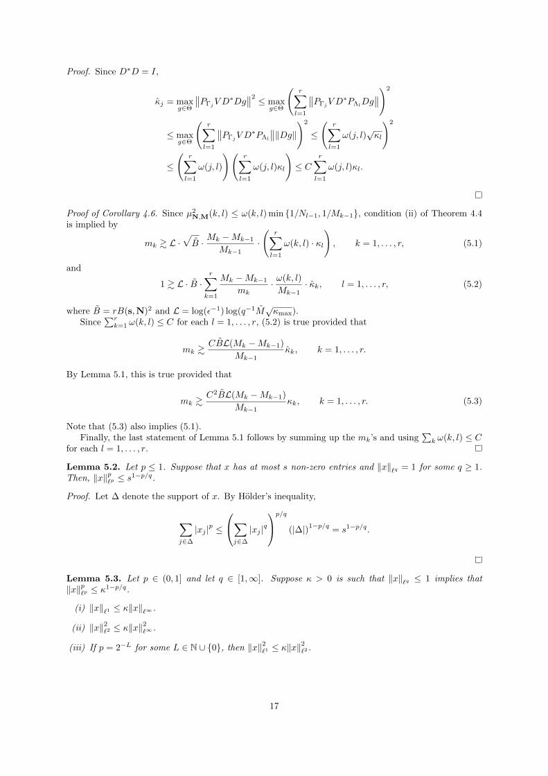
Proof. Since D∗D = I,

κj = maxg∈Θ

∥∥PΓjV D∗Dg

∥∥2 ≤ maxg∈Θ

(r∑l=1

∥∥PΓjV D∗PΛlDg

∥∥)2

≤ maxg∈Θ

(r∑l=1

∥∥PΓjV D∗PΛl

∥∥‖Dg‖)2

≤

(r∑l=1

ω(j, l)√κl

)2

≤

(r∑l=1

ω(j, l)

)(r∑l=1

ω(j, l)κl

)≤ C

r∑l=1

ω(j, l)κl.

Proof of Corollary 4.6. Since µ2N,M(k, l) ≤ ω(k, l) min 1/Nl−1, 1/Mk−1, condition (ii) of Theorem 4.4

is implied by

mk & L ·√B · Mk −Mk−1

Mk−1·

(r∑l=1

ω(k, l) · κl

), k = 1, . . . , r, (5.1)

and

1 & L · B ·r∑

k=1

Mk −Mk−1

mk· ω(k, l)

Mk−1· κk, l = 1, . . . , r, (5.2)

where B = rB(s,N)2 and L = log(ε−1) log(q−1M√κmax).

Since∑rk=1 ω(k, l) ≤ C for each l = 1, . . . , r, (5.2) is true provided that

mk &CBL(Mk −Mk−1)

Mk−1κk, k = 1, . . . , r.

By Lemma 5.1, this is true provided that

mk &C2BL(Mk −Mk−1)

Mk−1κk, k = 1, . . . , r. (5.3)

Note that (5.3) also implies (5.1).Finally, the last statement of Lemma 5.1 follows by summing up the mk’s and using

∑k ω(k, l) ≤ C

for each l = 1, . . . , r.

Lemma 5.2. Let p ≤ 1. Suppose that x has at most s non-zero entries and ‖x‖`q = 1 for some q ≥ 1.Then, ‖x‖p`p ≤ s1−p/q.

Proof. Let ∆ denote the support of x. By Holder’s inequality,

∑j∈∆

|xj |p ≤

∑j∈∆

|xj |qp/q

(|∆|)1−p/q= s1−p/q.

Lemma 5.3. Let p ∈ (0, 1] and let q ∈ [1,∞]. Suppose κ > 0 is such that ‖x‖`q ≤ 1 implies that‖x‖p`p ≤ κ1−p/q.

(i) ‖x‖`1 ≤ κ‖x‖`∞ .

(ii) ‖x‖2`2 ≤ κ‖x‖2`∞ .

(iii) If p = 2−L for some L ∈ N ∪ 0, then ‖x‖2`1 ≤ κ‖x‖2`2 .

17

Proof. Without loss of generality, first assume that ‖x‖`∞ = 1. Then, ‖x‖p`p ≤ κ. So, (i) follows because∑j

|xj | =∑j

|xj |p |xj |1−p ≤∑j

|xj |p ≤ κ,

and (ii) follows because ∑j

|xj |2 =∑j

|xj |p |xj |2−p ≤∑j

|xj |p ≤ κ.

To show (iii), assume (without loss of generality) that ‖x‖`2 = 1 and recall that p = 2−L. Then, byrepeatedly applying the Cauchy-Schwarz inequality,

‖x‖2`1 =

∑j

|xj |

2

≤∑j

|xj |p∑j

|xj |2(1−p/2) ≤ κ1−p/2‖x‖`2

∑j

|xj |2−2p

1/2

≤ κ1−p/2‖x‖1+1/2`2

∑j

|xj |2−4p

1/4

≤ κ1−p/2‖x‖1+1/2`2

∑j

|xj |2−2Lp

1/2L

= κ1−p/2‖x‖p`1 ,

and by dividing both sides of the inequality by ‖x‖p`1 , we obtain

‖x‖2(1−p/2)`1 ≤ κ1−p/2 =⇒ ‖x‖2`1 ≤ κ.

Corollary 5.4. In the notation of Definition 4.1, a direct application of the two lemmas presented above(with x := PΛlDD

∗y, l = 1, . . . , r) would yield the following results:

1. Lemma 5.2: if D was the analysis operator of an orthonormal basis (so that DD∗ = I) in Definition4.1, then κ(s,N) = s1 + · · ·+ sr.

2. Lemma 5.3 (i) : If y ∈ Σs,N and∥∥PΛjDD

∗y∥∥`∞

= 1, then∥∥PΛjDD∗y∥∥`1≤ κj(p,N, s), j = 1, . . . , r.

3. Lemma 5.3 (ii) : If y ∈ Σs,N and∥∥PΛjDD

∗y∥∥`∞

= 1, then∥∥PΛjDD∗y∥∥2

`2≤ κj(N, s, p), j = 1, . . . , r.

4. Lemma 5.3 (ii) : If y ∈ Σs,N and∥∥PΛjDD

∗y∥∥`2

= 1, then∥∥PΛjDD∗y∥∥2

`1≤ κj(N, s, p), j = 1, . . . , r.

Numerical example: the Haar frame

In the case where D is associated with a Haar frame on CN , it can be shown that if |supp(x)| = s thenDD∗x has at most O (s logN) nonzero entries (see [27]). Therefore, from Lemma 5.2, κ(N, s) . s log(N)where s = (sj)

rj=1 and s = s1 + . . .+ sr. In the case of a Haar frame, experimental results suggest that

the localized level sparsities κjj tend to follow a similar pattern to the level sparsities sj: Let D be

the discrete Haar frame, and let f ∈ R1024 be as shown on the right of Figure 5. Let ∆ be the supportof Df . Let S consist of 1000 randomly generated vectors, each supported on ∆. For each j = 0, . . . , 10,let Λj index all Haar framelet coefficients in the jth scale and let

κj = sup∥∥PΛjη∞

∥∥`1,∥∥PΛjη2

∥∥2

`1: η∞ = DD∗x/‖DD∗x‖`∞ , η2 = DD∗x/‖DD∗x‖`∞ , x ∈ S

. (5.4)

We also let sj = |∆ ∩ Λj |. The bar charts in Figure 5 show for each j = 0, . . . , 10, sj/ |Λj | (centreplot) and κj/ |Λj | (left plot). Note that κj merely approximate the localized level sparsities κj,because otherwise, we would need to consider all (s,N)-sparse support sets instead of just one supportset ∆ and we would also need to maximize over all vectors supported on ∆, instead of just 1000 randomlygenerated vectors. Nonetheless, Figure 5 provides some indication of the behaviour of the localized levelsparsities.

18

f Sparsity in levels Localized sparsity in levels

0 100 200 300 400 500 600 700 800 900 1000−10

−5

0

5

0 1 2 3 4 5 6 7 8 9 100

0.1

0.2

0.3

0.4

0.5

0.6

0.7

0.8

0.9

1

0 1 2 3 4 5 6 7 8 9 100

0.1

0.2

0.3

0.4

0.5

0.6

0.7

0.8

0.9

1

Figure 5: Left: the original vector. Centre: the level sparsities of Df at each scale. Right: theapproximate localized level sparsities at each scale, as defined in (5.4).

5.1 Intrinsic localization

As mentioned previously, many of the popular frames such as curvelets, shearlets and wavelet frames areintrinsically localized so that their Gram matrices are near diagonal. This property has been studied forwavelet frames in [26, 10, 18] and more recently for anisotropic systems such as shearlets and curveletsin [23, 24]. In this section, we will show how the property of intrinsic localization can yield estimates onthe localized sparsity term, κ, and the localized level sparsity terms, κj ’s. We first recall the notion ofintrinsic localization [22, 21].

Definition 5.5. Let H be a Hilbert space and let Ψ = ψjj∈N be a frame for H. Ψ is said to beintrinsically localized with respect to c > 0 and L ≥ 1 if

|〈ψj , ψk〉| ≤c

(1 + |j − k|)L, ∀j, k ∈ N.

Given ∆,Λ ⊆ N and p ∈ (L−1, 1], let

Ip(∆,Λ) = maxj∈∆

∑k∈Λ

|〈ψk, ψj〉|p .

Remark 5.1 Under this definition, wavelet frames have been shown to be intrinsically localized [10]with the parameter L being dependent on the regularity of the generating wavelets. For the anisotropicsystems studied in [23] and [24], the definition of intrinsic localization used is more complex than thedefinition presented above. However, the key idea of how to exploit this property to obtain bounds onthe localized sparsity values should still be applicable.

Remark 5.2 Given any ∆,Λ ⊆ N and p ∈ (L−1, 1], note that Lp > 1 and

Ip(∆,Λ) ≤ maxj∈∆

∑k∈Λ

c

(1 + |j − k|)Lp≤ 1 +

∫ ∞1

c

|x|Lpdx ≤ 1 +

c

Lp− 1.

So Ip(∆,Λ) is finite. Moreover, if we let

d = dist(∆,Λ) := mink∈∆,j∈Λ

|k − j| ≥ 1,

then

Ip(∆,Λ) ≤∫ ∞d

c

|x|Lpdx =

c

(Lp− 1) · dLp−1

The main result of this section is as follows.

19

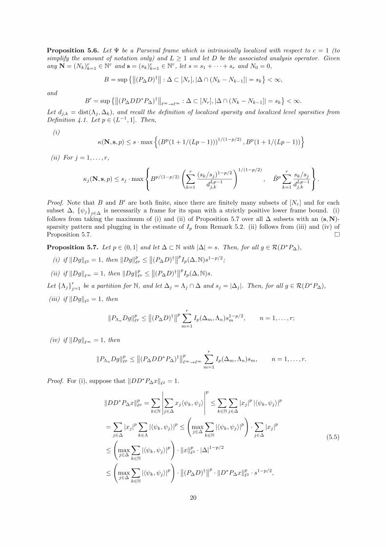
Proposition 5.6. Let Ψ be a Parseval frame which is intrinsically localized with respect to c = 1 (tosimplify the amount of notation only) and L ≥ 1 and let D be the associated analysis operator. Givenany N = (Nk)rk=1 ∈ Nr and s = (sk)rk=1 ∈ Nr, let s = s1 + · · ·+ sr and N0 = 0,

B = sup∥∥(P∆D)†

∥∥ : ∆ ⊂ [Nr], |∆ ∩ (Nk −Nk−1]| = sk<∞,

andB′ = sup

∥∥(P∆DD∗P∆)†

∥∥`∞→`∞ : ∆ ⊂ [Nr], |∆ ∩ (Nk −Nk−1]| = sk

<∞.

Let dj,k = dist(Λj ,∆k), and recall the definition of localized sparsity and localized level sparsities fromDefinition 4.1. Let p ∈ (L−1, 1]. Then,

(i)

κ(N, s, p) ≤ s ·max

(Bp(1 + 1/(Lp− 1)))1/(1−p/2)

, Bp(1 + 1/(Lp− 1))

(ii) For j = 1, . . . , r,

κj(N, s, p) ≤ sj ·max

Bp/(1−p/2)

(r∑

k=1

(sk/sj)1−p/2

dLp−1j,k

)1/(1−p/2)

, Bpr∑

k=1

sk/sj

dLp−1j,k

.

Proof. Note that B and B′ are both finite, since there are finitely many subsets of [Nr] and for eachsubset ∆, ψjj∈∆ is necessarily a frame for its span with a strictly positive lower frame bound. (i)

follows from taking the maximum of (i) and (ii) of Proposition 5.7 over all ∆ subsets with an (s,N)-sparsity pattern and plugging in the estimate of Ip from Remark 5.2. (ii) follows from (iii) and (iv) ofProposition 5.7.

Proposition 5.7. Let p ∈ (0, 1] and let ∆ ⊂ N with |∆| = s. Then, for all g ∈ R(D∗P∆),

(i) if ‖Dg‖`2 = 1, then ‖Dg‖p`p ≤∥∥(P∆D)†

∥∥pIp(∆,N)s1−p/2;

(ii) if ‖Dg‖`∞ = 1, then ‖Dg‖p`p ≤∥∥(P∆D)†

∥∥pIp(∆,N)s.

Let Λjrj=1 be a partition for N, and let ∆j = Λj ∩∆ and sj = |∆j |. Then, for all g ∈ R(D∗P∆),

(iii) if ‖Dg‖`2 = 1, then

‖PΛnDg‖p`p ≤

∥∥(P∆D)†∥∥p r∑

m=1

Ip(∆m,Λn)s1−p/2m , n = 1, . . . , r;

(iv) if ‖Dg‖`∞ = 1, then

‖PΛnDg‖p`p ≤

∥∥(P∆DD∗P∆)†

∥∥p`∞→`∞

r∑m=1

Ip(∆m,Λn)sm, n = 1, . . . , r.

Proof. For (i), suppose that ‖DD∗P∆x‖`2 = 1.

‖DD∗P∆x‖p`p =∑k∈N

∣∣∣∣∣∣∑j∈∆

xj〈ψk, ψj〉

∣∣∣∣∣∣p

≤∑k∈N

∑j∈∆

|xj |p |〈ψk, ψj〉|p

=∑j∈∆

|xj |p∑k∈Λ

|〈ψk, ψj〉|p ≤

(maxj∈∆

∑k∈N|〈ψk, ψj〉|p

)·∑j∈∆

|xj |p

≤

(maxj∈∆

∑k∈N|〈ψk, ψj〉|p

)· ‖x‖p`2 · |∆|

1−p/2

≤

(maxj∈∆

∑k∈N|〈ψk, ψj〉|p

)·∥∥(P∆D)†

∥∥p · ‖D∗P∆x‖p`2 · s1−p/2,

(5.5)

20

where we have applied the Cauchy-Schwarz inequality in the penultimate line. Therefore,

‖DD∗P∆x‖p`p ≤ I(∆,N)∥∥(P∆D)†

∥∥ps1−p/2.

To show (ii), if we instead assume that ‖DD∗P∆x‖`∞ = 1, then since

‖DD∗P∆x‖p`2 = ‖DD∗‖p`2‖x‖p`2 ≤ ‖DD

∗‖p`2sp/2,

by plugging this into the last line of (5.5), we obtain

‖DD∗P∆x‖p`p ≤ I(∆,Λ)∥∥(P∆D)†

∥∥ps.The proof of (iii) is similar to the above: if ‖D∗P∆x‖ = 1, then for each n = 1, . . . , r,

‖PΛnDD∗P∆x‖p`p ≤

r∑m=1

(maxj∈∆m

∑k∈Λ

|〈ψk, ψj〉|p)·∑j∈∆m

|xj |p

≤r∑

m=1

∑j∈∆m

(maxj∈∆m

∑k∈Λ

|〈ψk, ψj〉|p)· ‖P∆m

x‖p`2 · |∆m|1−p/2

≤∥∥(P∆D)†

∥∥p · r∑m=1

I(∆m,Λn) · s1−p/2m ,

(5.6)

Finally, to show (iv), if ‖D∗P∆x‖`∞ = 1, then for each n = 1, . . . , r,

‖PΛnDD∗P∆x‖p`p ≤

r∑m=1

(maxj∈∆m

∑k∈Λ

|〈ψk, ψj〉|p)·∑j∈∆m

|xj |p

≤r∑

m=1

∑j∈∆m

(maxj∈∆m

∑k∈Λ

|〈ψk, ψj〉|p)· ‖P∆mx‖

p`∞ · |∆m|

≤∥∥(P∆DD

∗P∆)†∥∥p`∞→`∞ ·

r∑m=1

I(∆m,Λn) · sm,

(5.7)

6 Conditions for stable and robust recovery

Given ∆ ⊂ N and some f ∈ H, the following proposition presents conditions under which one is guaran-teed robust and stable recovery up to

∥∥P⊥∆Df∥∥`1 .

Proposition 6.1 (Dual certificate). Let f ∈ H. Let ∆ ⊂ N be such that |∆| = s. Let W = R(D∗P∆).For r ∈ N, let q = qjrj=1 ∈ (0, 1]r and let Ωkrk=1 be disjoint subsets of N. Let Ω = Ω1 ∪ · · · ∪ Ωr.Suppose that

(i)∥∥QWV ∗(q−1

1 PΩ1⊕ · · · ⊕ q−1

r PΩr )V QW −QW∥∥ < 1

4 ,

(ii) supj∈N∥∥PjDQ⊥WV ∗(q−1

1 PΩ1⊕ · · · ⊕ q−1

r PΩr )V Q⊥WD

∗Pj∥∥ < 5

4 ,

and that there exists ρ = V ∗PΩw and L > 0 with the following properties.

(iii) ‖D∗P∆sgn(P∆Dx)−QWρ‖ ≤ q1/2/8,

(iv)∥∥P⊥∆DQ⊥Wρ∥∥`∞ ≤ 1/2,

(v) ‖w‖`2 ≤ L√κ.

Let y ∈ `2(N) be such that ‖PΩV f − y‖ ≤ δ. Then, any minimizer f ∈ H of (3.2) satisfies∥∥∥f − f∥∥∥H

. δ(q−1/2 + L

√κ)

+∥∥P⊥∆Df∥∥`1 . (6.1)

21

Proof. Since D is an isometry, D∗D is the identity on H. Given any g ∈ H,

Q⊥Wg = Q⊥WD∗Dg = Q⊥WD

∗P⊥∆Dg, (6.2)

since QW is the orthogonal projection onto R(D∗P∆). So, using the assumption that ‖D‖H→`2 ≤ 1, forany g ∈ H,

‖g‖ ≤ ‖QWg‖+∥∥Q⊥Wg∥∥ ≤ ‖QWg‖H +

∥∥P⊥∆Dg∥∥`1 .Now, let h = f − f . To bound ‖h‖H, it suffices to derive bounds for ‖QWh‖ and

∥∥P⊥∆Dh∥∥`1 .

Let VΩ,q = QWV∗(q−1

1 PΩ1⊕ · · · ⊕ q−1

r PΩr )V QW . We first observe that (i) implies that VΩ,q has abounded inverse on QW(H), with∥∥(QWV

∗(q−11 PΩ1

⊕ · · · ⊕ q−1r PΩr )V QW)−1

∥∥H→H ≤

4

3,

and ∥∥∥(q−1/21 PΩ1 ⊕ · · · ⊕ q−1/2

r PΩr )V QW

∥∥∥ ≤√5

4.

Observe also that‖PΩV h‖ ≤ ‖PΩV f − y‖+ ‖PΩV f − y‖ ≤ 2δ.

By applying the above observations, we have that

‖QWh‖ =∥∥∥V −1

Ω,qVΩ,qh∥∥∥

≤∥∥∥V −1

Ω,q

∥∥∥H

∥∥QWV ∗(q−11 PΩ1

⊕ · · · ⊕ q−1r PΩr )V (h−Q⊥W)h

∥∥≤ 4

3

(√

5 q−1/2 δ +

√5

4

∥∥∥(q−1/21 PΩ1

⊕ · · · ⊕ q−1/2r PΩr )V Q

⊥Wh∥∥∥) .

(6.3)

Also, by (ii),∥∥∥(q−1/21 PΩ1

⊕ · · · ⊕ q−1/2r PΩr )V Q

⊥Wh∥∥∥ =

∥∥∥(q−1/21 PΩ1

⊕ · · · ⊕ q−1/2r PΩr )V Q

⊥WD

∗P⊥∆Dh∥∥∥`2

≤ supj∈∆c

∥∥∥(q−1/21 PΩ1

⊕ · · · ⊕ q−1/2r PΩr )V Q

⊥WD

∗ej

∥∥∥`2

∥∥P⊥∆Dh∥∥`1 ≤√

5

4

∥∥P⊥∆Dh∥∥`1 .Plugging this into (6.3) yields

‖QWh‖H ≤ 2(q−1/2 δ +

∥∥P⊥∆Dh∥∥`1) . (6.4)

So, to bound ‖h‖H, it suffices to bound∥∥P⊥∆Dh∥∥`1 .

Observe that

‖Df‖`1 = ‖P⊥∆D(f + h)‖`1 + ‖P∆D(f + h)‖`1≥∥∥P⊥∆Dh∥∥`1 − ∥∥P⊥∆Df∥∥`1 + ‖P∆Df‖1 + Re 〈P∆Dh, sgn(P∆Df)〉

=∥∥P⊥∆Dh∥∥`1 − 2

∥∥P⊥∆Df∥∥`1 + ‖Df‖1 + Re 〈P∆Dh, sgn(P∆Df)〉.

Since f is a minimizer, we can deduce that∥∥P⊥∆Dh∥∥`1 ≤ |〈P∆Dh, sgn(P∆Df)〉|+ 2∥∥P⊥∆Df∥∥`1 .

Using the existence of ρ = V ∗PΩw and recalling that Q⊥W = Q⊥WD∗P⊥∆D from (6.2), we have that

|〈P∆Dh, sgn(P∆Df)〉| = |〈h,D∗sgn(P∆Df)〉|≤ |〈h,D∗sgn(P∆Df)−QWρ〉|+ |〈h, ρ〉|+

∣∣〈h,Q⊥Wρ〉∣∣≤ ‖QWh‖H‖D

∗sgn(P∆Df)−QWρ‖H + ‖PΩV h‖`2‖w‖`2 +∣∣〈D∗P⊥∆Dh,Q⊥Wρ〉∣∣

≤√q

8‖QWh‖H + 2δ L

√κ+

1

4

∥∥P⊥∆Dh∥∥`1≤ δ

(1

4+ 2L

√κ

)+

3

4

∥∥P⊥∆Dh∥∥`1 ,22

where we have used the bound on ‖QWh‖H from (6.4) to obtain the last inequality. Therefore,∥∥P⊥∆Dh∥∥`1 ≤ 8∥∥P⊥∆Df∥∥`1 + δ

(1 + 8L

√κ).

Finally, combining this with (6.4) yields

‖h‖H ≤ δ(

2q−1/2 + 3(1 + 8L

√κ))

+ 16∥∥P⊥∆Df∥∥`1 .

Proposition 6.2 (Dual certificate for the unconstrained problem). Consider the setting of Proposition

6.1 and assume that conditions (i)-(v) are satisfied. Let α > 0 and suppose that f ∈ H is a minimizer of

infg∈H

α‖Dg‖`1 + ‖PΩV g − y‖2`2 ,

where y ∈ `2(N) is such that ‖PΩV f − y‖ ≤ δ. Then,∥∥∥f − f∥∥∥H

.δ2

α+ α

(1√q

+ L√κ

)2

+ δ

(1√q

+ L√κ

)+∥∥P⊥∆Df∥∥`1 .

Thus, if α =√qδ, then ∥∥∥f − f∥∥∥

H. δ

(1√q

+ L√κ+√qL2κ

)+∥∥P⊥∆Df∥∥`1 .

Proof. Let h = f − f , just as in Proposition 6.1,

‖h‖H ≤ ‖QWh‖H +∥∥P⊥∆Dh∥∥`1

and it suffices to bound the two terms on the right side of the inequality. We first consider ‖QWh‖H.By applying assumptions (i) and (ii), we can proceed as in the proof of Proposition 6.1 to derive

‖QWh‖H ≤4

3

(√3

2q−1/2‖PΩV h‖`2 +

5

4

∥∥P⊥∆Dh∥∥`1). (6.5)

Then, by letting λ =∥∥∥y − PΩV f

∥∥∥`2

and observing that

‖PΩV h‖`2 ≤ ‖PΩV f − y‖`2 +∥∥∥PΩV f − y

∥∥∥`2≤ δ + λ,

we have that

‖QWh‖H ≤4

3

(√3

2q−1/2(δ + λ) +

5

4

∥∥P⊥∆Dh∥∥`1)

≤ 2

((δ + λ)√q

+∥∥P⊥∆Dh∥∥`1) .

(6.6)

To bound∥∥P⊥∆Dh∥∥`1 , first observe that

α∥∥∥Df∥∥∥

`1≥α∥∥P⊥∆Dh∥∥`1 − 2α

∥∥P⊥∆Df∥∥`1 + α‖Df‖`1 + αRe 〈P∆Dh, sgn(P∆Df)〉

+ λ2 − λ2 + ‖y − PΩV f‖2`2 − δ2.

Since f is a minimizer, it follows that α∥∥∥Df∥∥∥

`1+ λ2 ≤ α‖Df‖`1 + ‖y − PΩV f‖2`2 and therefore,

α∥∥P⊥∆Dh∥∥`1 + λ2 ≤ 2α

∥∥P⊥∆Df∥∥`1 + α |〈P∆Dh, sgn(P∆Df)〉|+ δ2. (6.7)

23

In the same way as in the proof of Proposition 6.1, we may apply the properties of the dual certificateρ = V ∗PΩw to bound |〈P∆Dh, sgn(P∆Df)〉|, so that the following holds.

|〈P∆Dh, sgn(P∆Df)〉| ≤√q

8‖QWh‖H + ‖PΩV h‖`2‖w‖`2 +

1

4

∥∥P⊥∆Dh∥∥`1 .By inserting the bound from (6.6), recalling that ‖PΩV h‖`2 ≤ δ + λ and that ‖w‖`2 ≤ L

√κ, it follows

that

|〈P∆Dh, sgn(P∆Df)〉| ≤ (δ + λ)

(1

4+ L√κ

)+

1

2

∥∥P⊥∆Dh∥∥`1 .Plugging this bound into (6.7) now yields

λ2 +α

2

∥∥P⊥∆Dh∥∥`1 ≤ 2α∥∥P⊥∆Df∥∥`1 + α(δ + λ)

(1

4+ L√κ

)+ δ2. (6.8)

This implies that

λ2 − α(

1

4+ L√κ

)λ− δ2 − αδ

(1

4+ L√κ

)≤ 0

and by applying the quadratic formula and observing that λ ≥ 0, it follows that

λ ≤α/4 + Lα

√κ+

√(α/4 + Lα

√κ)2 + 4

(δ2 + αδ(1/4 + L

√κ) + 2α

∥∥P⊥∆Df∥∥`1)2

.

Note that ‖·‖`2 ≤ ‖·‖`1 , and so,

λ ≤ α/4 + Lα√κ+ δ +

√αδ(1/4 + L

√κ) +

√2α∥∥P⊥∆Df∥∥`1

≤ α/4 + Lα√κ+ δ + α(1/8 + L

√κ/2) + δ/2 +

√2α∥∥P⊥∆Df∥∥`1

=3α

2(1/4 + L

√κ) +

3δ

2+√

2α∥∥P⊥∆Df∥∥`1 ,

(6.9)

where the second inequality comes from the fact that√ab ≤ (a + b)/2 for any a, b ≥ 0. We also know

from (6.8) that ∥∥P⊥∆Dh∥∥`1 ≤ 4∥∥P⊥∆Df∥∥`1 + (δ + λ)

(1

2+ 2L

√κ

)+

2δ2

α.

By combining this with the bound from (6.6),

‖h‖H ≤ ‖QWh‖H +∥∥P⊥∆Dh∥∥`1

≤ 3

(4∥∥P⊥∆Df∥∥`1 + δ

(1

2+ 2L

√κ

)+

2δ2

α

)+

2δ√q

+

(2√q

+ 3

(1

2+ 2L

√κ

))λ

.∥∥P⊥∆Df∥∥`1 + δ(1 + L

√κ) +

δ2

α+

δ√q

+

(1√q

+ 1 + L√κ

)λ.

Recalling (6.9),(1√q

+ 1 + L√κ

)λ .

(1√q

+ 1 + L√κ

)(α(1 + L

√κ) + δ +

√α∥∥P⊥∆Df∥∥`1

).

(1√q

+ 1 + L√κ

)(α(1 + L

√κ) + δ

)+α

q+∥∥P⊥∆Df∥∥`1 + α(1 + L

√κ)

≤ α(

1√q

+ 1 + L√κ

)2

+ δ

(1√q

+ 1 + L√κ

)+∥∥P⊥∆Df∥∥`1 .

Therefore,

‖h‖H ≤δ2

α+ α

(1√q

+ 1 + L√κ

)2

+ δ

(1√q

+ 1 + L√κ

)+∥∥P⊥∆Df∥∥`1 .

24

7 Overview of the proof of Theorem 4.4

The remainder of this paper is focussed on the proof of Theorem 4.4, and we begin by setting somenotation which will be used throughout.

Let V,D ∈ B(H, `2(N)) be isometries. Let f ∈ H. For r ∈ N, M ∈ N and N ∈ N, let N = Nkrk=1 ∈Nr, M = Mkrk=1 ∈ Nr, s = skrk=1 ∈ Nr, m = mkrk=1 ∈ Nr, with

• 0 = M0 < M1 < · · · < Mr =: M , and let Γk = (Mk−1,Mk] ∩ N and Ωk ∼ Ber(qk,Γk).

• 0 = N0 < N1 < · · · < Nr =: N , and let Λk = (Nk−1, Nk] ∩ N for k = 1, . . . , r − 1 and Λr =(Nr−1,∞) ∩ N.

• mk ≤Mk −Mk−1 and let q = qjrj=1 ∈ (0, 1]r with qj = mj/(Mj −Mj−1).

• sk ≤ Nk−Nk−1 and let ∆ ⊂ [N ] be such that |∆| = s1 + · · ·+sr =: s and ∆k = Λk∩∆, |∆k| = sk.Let W = R(D∗P∆).

For some p ∈ (0, 1], we will write κ = κjrj=1 with κl = κl(N, s, p) and κl = κl(N,M,κ) for each

l = 1, . . . , r. Let κmin = rminrl=1 κl and κmax = rmaxrl=1 κl. Note that κmin ≤∑rl=1 κj ≤ κmax.

We also define T ∈ B(`2(N), `2(N)) such that given any x = (xj)j∈N ∈ `2(N),

Tx = y, yj =xj

max

1,√rκk , j ∈ Λk, k = 1, . . . , r.

Observe that T is an invertible operator, ‖T‖ ≤ 1/√κmin and

∥∥T−1∥∥ ≤ √κmax.

7.1 Outline of the proof

To prove Theorem 4.4, it suffices to show that conditions (i)-(v) of Proposition 6.1 are satisfied with highprobability whenever the sampling scheme is the multilevel sampling scheme Ω = ΩM,m described inTheorem 4.4. To this end, we first remark that it has become customary in compressed sensing theoryto deduce recovery statements for uniform sampling models by first proving statements based on somealternative sampling model which is easier to analyse. One approach, considered in [8, 2, 1] is to considera Bernoulli sampling model, defined below.

Definition 7.1. Let M = Mkrk=1 with 0 = M0 < M1 < · · · < Mr. Let ΩBerM,m := ΩBer

1 ∪ · · · ∪ ΩBerr ,

where ΩBerk := δj · j : j ∈ Γk with Γk = N∩ (Mk−1, · · · ,Mk], and δj are independent random variables

such that P(δj = 1) = mk/(Mk − Mk−1) and P(δj = 0) = 1 − mk/(Mk − Mk−1). The Bernoullisampling set ΩBer

k described will be denoted by ΩBerk ∼ Ber(mk/(Mk − Mk−1),Γk) and we say that

ΩBerM,m = ΩBer

1 ∪ · · · ∪ ΩBerr is a Bernoulli (M,m)-sampling scheme.

As explained in [8, II.C] (see also [19]), the probability that one of the conditions of Proposition6.1 fails for Ω = ΩM,m chosen uniformly at random is up to a constant bounded from above by theprobability that one of these conditions fails under the Bernoulli (M,m)-sampling scheme, Ω = ΩBer

M,m.So, to prove Theorem 4.4, it suffices to show that conditions (i) to (v) of Proposition 6.1 hold with

probability exceeding (1− ε) with Ω = ΩBerM,m satisfying the following assumption.

Assumption 7.2. Let L =(log(ε−1) + 1

)log(Mq−1κ

1/2max‖DD∗‖`∞→`∞) and

B = max

∥∥DQ⊥WD∗∥∥`∞→`∞ ,√√√√‖DQWD∗‖`∞→`∞ r

maxl=1

r∑t=1

∥∥PΛlDQR(D∗P∆)D∗PΛt

∥∥`∞→`∞

.

Let

M = min

i ∈ N : max

j≥i

∥∥P[M ]V D∗ej∥∥`2≤ q

8√κmax

, maxj≥i

∥∥∥QR(D∗P[N])D∗ej

∥∥∥ ≤ √5q

4

,

Suppose that

25

(a)∥∥∥DQWV ∗P⊥[M ]V QWD

∥∥∥`2→`2

≤√

κmin

2κmaxlog−1/2(4q−1√κmaxM).

(b)∥∥DQ⊥WV ∗P[M ]V QWD

∗T−1∥∥`2→`∞ ≤

18√κmax

.

(c) For k = 1, . . . , r,

qk &√rLB

r∑l=1

µ2N,M(k, l)κl.

(d) For k = 1, . . . , r, qk ≥ L qk with qkrk=1 satisfying

1 & r B2r∑

k=1

(q−1k − 1)µ2

N,M(k, j) κk, j = 1, . . . , r.

Note that this assumption is strictly weaker than the assumptions of Theorem 4.4, and by showingthat conditions (i) to (v) of Proposition 6.1, we will prove that the error bound (6.1) holds for onesupport set ∆. So, by ensuring that the conditions of this assumption hold over all ∆ sets which are(N, s) sparse patterns (as required by Theorem 4.4), we can conclude that (6.1) holds for any (N, s)sparse support sets.

Under this assumption,

• §9 will show that conditions (iii) to (v) of Proposition 6.1 are satisfied with probability exceeding1− 5ε/6;

• §10 will show that conditions (i) and (ii) of Proposition 6.1 are satisfied with probability exceeding1− ε/6;

• §8 will present some preliminary results for use in §9 and §10.

The proof of Corollary 4.5 Once we have shown that the conditions of Proposition 6.1 hold withprobability exceeding 1− ε, the conclusion of Proposition 6.2 automatically follows and we may concludeCorollary 4.5.

8 Preliminary results

In this section, we present four propositions which will be applied to show that the conditions of Proposi-tion 6.1 are satisfied with high probability under the conditions of Theorem 4.4 with a Bernoulli samplingscheme. The results in this section are derived using Talagrand’s inequality and Bernstein inequalities(for random variables and random matrices) which we state below.

Theorem 8.1. (Talagrand [32, Cor. 7.8]) There exists a number K with the following property. Considern independent random variables Xi valued in a measurable space Ω and let F be a (countable) class ofmeasurable functions on Ω. Let Z be the random variable Z = supf∈F

∑i≤n f(Xi) and define

S = supf∈F‖f‖∞, V = sup

f∈FE

∑i≤n

f(Xi)2

.

If E(f(Xi)) = 0 for all f ∈ F and i ≤ n, then, for each t > 0, we have

P(|Z − E(Z)| ≥ t) ≤ 3 exp

(− 1

K

t

Slog

(1 +

tS

V + SE(Z)

)),

where Z = supf∈F |∑i≤n f(Xi)|.

26

Theorem 8.2 (Bernstein inequality for random variables [19]). Let Z1, . . . , ZM ∈ C be independentrandom variables with zero mean such that |Zj | ≤ K almost surely for all l = 1, . . . ,M and some

constant K > 0. Assume also that∑Mj=1 E |Zj |

2 ≤ σ2 for some constant σ2 > 0. Then for t > 0,

P

∣∣∣∣∣∣M∑j=1

Zj

∣∣∣∣∣∣ ≥ t ≤ 4 exp

(− t2/4

σ2 +Kt/(3√

2)

).

If Z1, . . . , ZM ∈ R are real instead of complex random variables, then

P

∣∣∣∣∣∣M∑j=1

Zj

∣∣∣∣∣∣ ≥ t ≤ 2 exp

(− t2/2

σ2 +Kt/3

).

Theorem 8.3 (Bernstein inequality for rectangular matrices [40]). Let Z1, . . . , ZM ∈ Cd1×d2 be inde-pendent random matrices such that EZj = 0 for each j = 1, . . . ,M and ‖Zj‖2→2 ≤ K almost surely foreach j = 1, . . . ,M and some constant K > 0. Let

σ2 := max

∥∥∥∥∥∥M∑j=1

E(ZjZ∗j )

∥∥∥∥∥∥`2→`2

,

∥∥∥∥∥∥M∑j=1

E(Z∗jZj)

∥∥∥∥∥∥`2→`2

.

Then, for t > 0,

P

∥∥∥∥∥∥M∑j=1

Zj

∥∥∥∥∥∥`2→`2

≥ t

≤ 2(d1 + d2) exp

(−t2/2

σ2 +Kt/3

)Proposition 8.4. Let g ∈ W and let α > 0 and γ ∈ [0, 1]. Suppose that∥∥TD(QWV

∗P[M ]V QW −QW)D∗T−1∥∥`2→`2 ≤ α/2. (8.1)

ThenP(∥∥TD(QWV

∗(q−11 PΩ1

⊕ · · · ⊕ q−1r PΩr )V QW −QW)g

∥∥`2≥ α‖TDg‖`2

)≤ γ

provided that√rB log

(3

γ

) r∑l=1

µ2N,M(k, l)κl . α, k = 1, . . . , r, (8.2)

and

rB2 log

(3

γ

) r∑k=1

(q−1k − 1)µ2

N,M(k, l) κk . α2, l = 1, . . . , r, (8.3)

where

B2 = ‖DQWD∗‖`∞→`∞r

maxl=1

r∑t=1

‖PΛlDQWD∗PΛt‖`∞→`∞ .

Proof. Without loss of generality, assume that ‖TDg‖`2 = 1. Let δjMj=1 be random Bernoulli variables

such that P(δj = 1) = qj where qj = qk for j = Mk−1 + 1, . . . ,Mk. Then,

TD(QWV∗(q−1

1 PΩ1 ⊕ · · · ⊕ q−1r PΩr )V QW −QW)g

=

M∑j=1

(q−1j δj − 1)TDQWV

∗(ej ⊗ ej)V QWg + TD(QWV∗P[M ]V QW −QW)g,

where ⊗ is the Kronecker product. Since D∗D = I and since (8.1) holds by assumption,∥∥TD(QWV∗P[M ]V QW −QW)g

∥∥`2

=∥∥TD(QWV

∗P[M ]V QW −QW)D∗T−1TDg∥∥`2

≤∥∥TD(QWV

∗P[M ]V QW −QW)D∗T−1∥∥`2→`2 ≤ α/2.

27

So, it suffices to show that

P

∥∥∥∥∥∥M∑j=1

Yj

∥∥∥∥∥∥`2

≥ α/2

≤ γ,where for each j = 1, . . . ,M , Yj = (q−1

j δj − 1)DQWV∗(ej ⊗ ej)V g. We will aim to apply Talagrand’s

inequality (Theorem 8.1) to obtain this probability bound.Let G be a countable set of vectors in the unit ball of `2(N) and for each ζ ∈ G, define the linear

functionals ζ1, ζ2 : `2(N)→ R by

ζ1(y) = Re 〈y, ζ〉, ζ2(y) = −Re 〈y, ζ〉, ∀y ∈ `2(N).

Let F =ζ1, ζ2 : ζ ∈ G

. Then, Z := supf∈F

∑Mj=1 f(Yj) =

∥∥∥∑Mj=1 Yj

∥∥∥`2

.

• To bound S = maxj ‖Yj‖`2 :

‖Yj‖`2 ≤ q−1j ‖TDQWV

∗(ej ⊗ ej)V g‖`2 = q−1j sup‖x‖`2=1

|〈TDQWV ∗(ej ⊗ ej)V g, x〉|

= q−1j sup‖x‖`2=1

|〈V g, ej〉〈TDQWV ∗ej , x〉|

For each j ∈ Γk,

|〈V g, ej〉| = |〈V D∗Dg, ej〉| ≤r∑l=1

|〈V D∗PΛlDg, ej〉| ≤r∑l=1

µ(PΓkV D∗PΛl)‖PΛlDg‖`1 .

Observe that ‖TDg‖`2 = 1 implies ‖PΛlDg‖`2 ≤√rκl for each l = 1, . . . , r. Furthermore, by (4)

of Corollary 5.4, this implies that ‖PΛlDg‖`1 ≤ κl√r. So, it follows that

|〈V g, ej〉| ≤√r

r∑l=1

µ(PΓkV D∗PΛl)κl.

Also, if ‖x‖`2 = 1,

|〈TDQWV ∗ej , x〉|2 ≤r∑l=1

‖PΛlTDQWV∗ej‖2`2 =

r∑l=1

1

rκl‖PΛlDQWD

∗DV ∗ej‖2`2

≤r∑l=1

1

rκl‖PΛlDQWD

∗‖2`∞→`2‖DV∗ej‖2`∞ ≤ ‖DQWD

∗‖2`∞→`∞µ2(PΓkV D),

(8.4)

where the last inequality follows because ‖PΛlDf‖2`2 ≤ κl for all f ∈ W with ‖Df‖`∞ ≤ 1.

Therefore,

maxj‖Yj‖`2 ≤

rmaxk=1‖DQWD∗‖`∞→`∞

√r

r∑l=1

µ2N,M(k, l)κl.

• To bound V = supf∈F E∑Mj=1 f(Yj)

2 = supζ∈G E∑Mj=1 |〈ζ, Yj〉|

2:

V ≤ supζ∈G

M∑j=1

(q−1j − 1) |〈ej , V g〉|2 |〈V ∗ej , QWD∗Tζ〉|2

≤ supζ∈G

r∑k=1

(q−1k − 1)‖PΓkV g‖

2`2 maxj∈Γk

|〈V ∗ej , QWD∗Tζ〉|2

≤r∑

k=1

(q−1k − 1)‖PΓkV g‖

2`2 maxj∈Γk

‖TDQWV ∗ej‖2`2 .

(8.5)

28

By combining ‖PΛlDg‖`2 ≤√rκl (which follows from ‖TDg‖`2 = 1) with the definition of κk, we

obtain ‖PΓkV g‖2`2 ≤ rκk. Also, for each j ∈ Γk,

‖TDQWV ∗ej‖2`2 =

r∑t=1

1

rκt‖PΛtDQWV

∗ej‖2`2

=

r∑t=1

1

rκt‖PΛtDQWD

∗‖`∞→`2‖DV∗ej‖`∞‖PΛtDQWV

∗ej‖`2

≤r∑t=1

1

r√κt‖DQWD∗‖`∞→`∞‖DV

∗ej‖`∞r∑l=1

‖PΛtDQWD∗Λl‖`∞→`2‖PΛlV

∗ej‖`∞

≤r∑t=1

1

r‖DQWD∗‖`∞→`∞

r∑l=1

‖PΛtDQWD∗Λl‖`∞→`∞µN,M(k, l)

where we have used, from the definition of the κj ’s, ‖PΛtDf‖`2 ≤√κt whenever t = 1, . . . , r,

f ∈ W and ‖Df‖`∞ ≤ 1. Therefore,

V ≤ r‖DQWD∗‖`∞→`∞r∑l=1

r∑k=1

(q−1k − 1)κkµ

2N,M(k, l)

r∑t=1

1

r‖PΛtDQWD

∗PΛl‖`∞→`∞

≤ rB2 rmaxl=1

r∑k=1

(q−1k − 1)µ2

N,M(k, l) κk,

where we have applied

1

r‖DQWD∗‖`∞→`∞

r∑l=1

r∑t=1

‖PΛtDQWD∗PΛl‖`∞→`∞

≤ ‖DQWD∗‖`∞→`∞r

maxl=1

r∑t=1

‖PΛlDQWD∗PΛt‖`∞→`∞ =: B2.

• To bound E(Z) = E∥∥∥∑M

j=1 Yj

∥∥∥:

E

∥∥∥∥∥∥M∑j=1

Yj

∥∥∥∥∥∥2

`2

=

M∑j=1

E‖Yj‖2`2 =

M∑j=1

(q−1j − 1)‖TDQWV ∗ej‖2`2 |〈V g, ej〉|

2

≤r∑

k=1

(q−1k − 1)‖PΓkV g‖

2`2 maxj∈Γk

‖TDQWV ∗ej‖2`2 .

This is the same upper bound as obtained in (8.5), so from the bound on V, we have that

E

∥∥∥∥∥∥M∑j=1

Yj

∥∥∥∥∥∥2

`2

≤ B2 rmaxl=1

r∑k=1

(q−1k − 1)µ2

N,M(k, l) κk.

Finally, by Jensen’s inequality,

E

∥∥∥∥∥∥M∑j=1

Yj

∥∥∥∥∥∥ ≤√√√√√√E

∥∥∥∥∥∥M∑j=1

Yj

∥∥∥∥∥∥2

`2

≤√√√√B2 r

maxl=1

r∑k=1

(q−1k − 1)µ2

N,M(k, l) κk.

Let C = max C1, 4C2/α, where

C1 = ‖DQWD∗‖`∞→`∞√r

rmaxk=1

r∑l=1

µN,M(k, l)κl,

29

and

C2 = rB2 rmaxl=1

r∑k=1

(q−1k − 1)µ2

N,M(k, l) κk.

Note that C ≥ S, αC/4 ≥ V. Suppose that C2 ≤ α2/16, then E(Z) ≤ α/4, since (E(Z))2 ≤ C2. By

applying Talagrand’s inequality with the upper bound of C ≥ S and E(Z) ≤ α/4,

P(Z ≥ α

2

)≤ P

(Z ≥ α

4+ E(Z)

)≥ P

(|Z − E(Z)| ≤ α

4

)≤ 3 exp

(− α

4KClog

(1 +

Cα/4

V + Cα/4

))≤ 3 exp

(− α

4KClog

(1 +

Cα/4

Cα/4 + Cα/4

))≤ 3 exp

(− α

4KClog

(3

2

)),

where K is the constant from Talagrand’s inequality. So, P(Z ≥ α

2

)≤ γ provided that

C log

(3

γ

)≤ α

4Klog

(3

2

).

as well as C2 ≤ α2/16. Therefore, the require result would follow provided that

‖DQWD∗‖`∞→`∞√r log

(3

γ

) r∑l=1

µN,M(k, l)κl ≤α

4Klog

(3

2

), k = 1, . . . , r,

and

rB2 log

(3

γ

) r∑k=1

(q−1k − 1)µ2

N,M(k, l) κk ≤α2

16min

1,

1

Klog

(3

2

), l = 1, . . . , r.

Proposition 8.5. Fix g ∈ H and let α > 0 and γ ∈ [0, 1]. Suppose that∥∥DQ⊥WV ∗P[M ]V QWD∗T−1

∥∥`2→`∞ ≤

α

2. (8.6)

Let B =∥∥DQ⊥WD∗∥∥`∞→`∞ . Let

M = min

i ∈ N : max

j≥i2√κmax ·

rmaxk=1

q−1k ·

∥∥P[M ]V D∗ej∥∥`2≤ α

, κmax = rmax κjrj=1 .

Then M is finite and

P(∥∥P⊥∆DQ⊥WV ∗(q−1

1 PΩ1⊕ · · · ⊕ q−1

r PΩr )V QWg∥∥`∞≥ α‖TDg‖`2

)≤ γ,

provided that

√r B log

(4M

γ

)q−1k

r∑l=1

µ2N,M(k, l)κl . α, k = 1, . . . , r

and

r B2 log

(4M

γ

)r∑

k=1

(q−1k − 1)µ2

N,M(k, j) κk . α2, j = 1, . . . , r.

Proof. Without loss of generality, assume that ‖TDg‖`2 = 1. Let δjMj=1 be random Bernoulli variables

such that P(δj = 1) = qj where qj = qk for j = Mk−1 + 1, . . . ,Mk. Observe that

Q⊥W = Q⊥WD∗D = Q⊥WD

∗P⊥∆D,

30

so we have that

P⊥∆DQ⊥WV

∗(q−11 PΩ1 ⊕ · · · ⊕ q−1

r PΩr )V g

=

M∑j=1

(q−1j δj − 1)P⊥∆DQ

⊥WD

∗P⊥∆DV∗(ej ⊗ ej)V g + P⊥∆Q

⊥WV

∗P[M ]V QWD∗T−1TDg.

Since∥∥P⊥∆DQ⊥WV ∗P[M ]V QWD

∗T−1∥∥`2→`∞ ≤ α/2, it suffices to show that

P

∥∥∥∥∥∥M∑j=1

(q−1j δj − 1)P⊥∆DQ

⊥WV

∗(ej ⊗ ej)V g

∥∥∥∥∥∥`∞

> α/2

≤ γ.For each i ∈ ∆c and j = 1, . . . ,M , let

Zij = (q−1j δj − 1)〈P⊥∆DQ⊥WV ∗(ej ⊗ ej)V Dg, ei〉.

For each i ∈ ∆c, we will first apply Bernstein’s inequality (Theorem 8.2) to consider upper bounds for

P(∣∣∣∑M

j=1 Zij

∣∣∣ ≥ α). Observe that

E(∣∣Zij∣∣2) = (q−1

j − 1)|〈P⊥∆DQ⊥WV ∗(ej ⊗ ej)V g, ei〉|2

= (q−1j − 1)|〈V ∗ej , Q⊥WP⊥∆Dei〉|2|〈ej , V g〉|2.

Let B =∥∥DQ⊥WD∗∥∥`∞→`∞ , Then,

M∑j=1

E(∣∣Zij∣∣2) ≤ sup

‖α‖`1≤B

r∑k=1

(q−1k − 1)‖PΓkV D

∗α‖2`∞‖PΓkV g‖2`2

≤ B sup‖α‖`1≤B

r∑k=1

(q−1k − 1)µ(PΓkV D

∗)‖PΓkV D∗α‖`∞‖PΓkV g‖

2`2

≤ B sup‖α‖`1≤B

r∑k=1

(q−1k − 1)µ(PΓkV D

∗)∑l∈N|αl| ‖PΓkV D

∗el‖`∞‖PΓkV g‖2`2

= B sup‖α‖`1≤B

∑l∈N|αl|

r∑k=1

(q−1k − 1)µ(PΓkV D

∗)‖PΓkV D∗el‖`∞‖PΓkV g‖

2`2

≤ B2 supl∈N

r∑k=1

(q−1k − 1)µ(PΓkV D

∗)‖PΓkV D∗el‖`∞‖PΓkV g‖

2`2

≤ B2 rmaxj=1

r∑k=1

(q−1k − 1)µ2

N,M(k, j)‖PΓkV g‖2`2

≤ rB2 rmaxj=1

r∑k=1

(q−1k − 1)µ2

N,M(k, j)κk =: σ2,

(8.7)

where the last line follows because ‖TDg‖`2 = 1 implies that ‖PΛkDg‖`2 ≤√rκk, and by definition of

κk, ‖PΓkV g‖2`2 ≤ rκk.

Also, we have that∣∣Zij∣∣ ≤ q−1j |〈V

∗ej , Q⊥WD

∗ei〉||〈ej , V D∗Dg〉|

≤ rmaxk=1

q−1k µ(PΓkV Q

⊥WD

∗P⊥∆ )

r∑l=1

µ(PΓkV D∗PΛl) ‖PΛlDg‖`1

≤∥∥DQ⊥WD∗∥∥`∞→`∞ r

maxk=1

q−1k

r∑l=1

µN,M(k, l) ‖PΛlDg‖`1

≤√r∥∥DQ⊥WD∗∥∥`∞→`∞ r

maxk=1

q−1k

r∑l=1

µN,M(k, l)κl =: K,

31

where the last line follows because ‖PΛlDg‖`2 ≤√rκl along with (4) of Corollary 5.4 implies that

‖PΛlDg‖`1 ≤√rκl.

Let Υ ⊂ N be such that

P

supi∈Υ

∣∣∣∣∣∣M∑j=1

Zij

∣∣∣∣∣∣ ≥ α = 0

and suppose that |Υc| ≤ M . Then, by Theorem 8.2 and the union bound,

P

supi∈∆c

∣∣∣∣∣∣M∑j=1

Zij

∣∣∣∣∣∣ ≥ α

2

≤ P

supi∈Υc

∣∣∣∣∣∣M∑j=1

Zij

∣∣∣∣∣∣ ≥ α

2

≤ 4 |Υc| exp

(− α2/16

σ2 +Kα/(6√

2)

),

which is true provided that

log

(4M

γ

)σ2 ≤ α2

32, log

(4M

γ

)K ≤ α

8.

which are simply the assumptions of this theorem.It remains to show that such as set Υc exists: First note that ‖Dg‖ ≤

∥∥T−1∥∥‖TDg‖ ≤ √κmax with

κmax = rmax κjrj=1. So, using the fact that D and V are isometries and hence of norm 1, notice that∣∣∣∣∣∣M∑j=1

Zij

∣∣∣∣∣∣ =∣∣〈(q−1

k − 1)P⊥∆DQ⊥WV

∗(q−11 PΩ1

⊕ · · · ⊕ q−1r PΩr )V g, ei〉

∣∣≤ ‖Dg‖`2

∥∥DQWV ∗(q−11 Ω1 ⊕ · · · q−1

r Ωr)V Q⊥WD

∗P⊥∆ ei∥∥`2

≤√κmax

rmaxk=1

q−1k

∥∥P[M ]V Q⊥WD

∗ei∥∥`2→ 0

as i→∞ since P[M ]V Q⊥WD

∗ is of finite rank. Thus, for α > 0, it suffices to let

Υc :=

i ∈ N :

√κmax

rmaxk=1

q−1k

∥∥P[M ]V Q⊥WD

∗ei∥∥`2≥ α

which is a finite set. To conclude this proof, observe that |Υc| ≤ M <∞.

Proposition 8.6. Let α > 0 and γ ∈ [0, 1]. Suppose that∥∥∥QWV ∗P⊥[M ]V QW

∥∥∥H→H

≤ α/2. (8.8)

Then,P(∥∥QWV ∗(q−1

1 PΩ1⊕ · · · ⊕ q−1

r PΩr )V QW −QWV ∗V QW∥∥H→H ≥ α

)≤ γ,

provided that

qk & α−2 log

(4M

γ

)r∑l=1

µ2N,M(k, l)κl, k = 1, . . . , r.

Proof. Let qj = qk for j ∈ Γk. Let δjrj=1 be Bernoulli random variables such that P(δj = 1) = qj .

∥∥QWV ∗(q−11 PΩ1

⊕ · · · ⊕ q−1r PΩr )V QW −QWV ∗V QW

∥∥ ≤∥∥∥∥∥∥M∑j=1

q−1j δjQWV

∗(ej ⊗ ej)V QW

∥∥∥∥∥∥≤

∥∥∥∥∥∥M∑j=1

(q−1j δj − 1)DQWV

∗(ej ⊗ ej)V QWD∗∥∥∥∥∥∥+

∥∥∥QWV ∗P⊥[M ]V QW

∥∥∥≤

∥∥∥∥∥∥M∑j=1

(q−1j δj − 1)DQWV

∗(ej ⊗ ej)V QWD∗∥∥∥∥∥∥+ α/2.

32

Let

U =

M∑j=1

(q−1j δj − 1)(ej ⊗ ej).

Then, for each J ∈ N, ‖DQWV ∗UV QWD‖ is bounded above by∥∥P[J]DQWV∗UV QWD

∗P[J]

∥∥+∥∥∥DQWV ∗UV QWD∗P⊥[J]

∥∥∥+∥∥∥P⊥[J]DQWV

∗UV QWD∗∥∥∥

≤∥∥P[J]DQWV

∗UV QWD∗P[J]

∥∥+ 2∥∥∥P⊥[J]DQW

∥∥∥‖U‖≤∥∥P[J]DQWV

∗UV QWD∗P[J]

∥∥+ 2q−1∥∥∥P⊥[J]DQW

∥∥∥where q = min qjrj=1. Note that since DQW has finite rank,

∥∥∥P⊥[J]DQW

∥∥∥→ 0 as J →∞. Let

M = minj ∈ N : 8

∥∥∥P⊥[j]DQW∥∥∥ ≤ qα .Then, it suffices to show that

P(∥∥∥P[M ]DQWV

∗UV QWD∗P[M ]

∥∥∥ > α/4)≤ γ

For each j = 1, . . . ,M , define Zj = (q−1j δj − 1)P[M ]DQWV

∗(ej ⊗ ej)V QWD∗P[M ]. We will aim to applyTheorem 8.3 to derive the following.

P

∥∥∥∥∥∥M∑j=1

Zj

∥∥∥∥∥∥ ≥ α

4

≤ γ.Notice that ZjMj=1 are independent mean-zero matrices. Let ξj = P[M ]DQWV

∗ej . Then,

‖Zj‖ ≤ q−1j

∥∥ξj ⊗ ξj∥∥ ≤ q−1j ‖ξj‖

2.

To bound this, note that for each j = 1, . . . ,M ,

‖ξj‖2 = supα∈CM

|〈DQWV ∗ej , α〉|2 = supα∈CM ,‖α‖`2=1

|〈DQWD∗DV ∗ej , α〉|2

≤ supα∈CM ,‖α‖`2=1

r∑l=1

|〈DQWD∗PΛlDV∗ej , α〉|2

≤ supα∈CM ,‖α‖`2=1

r∑l=1

‖PΛlDV∗ej‖2`∞‖PΛlDQWD

∗α‖2`1

≤ supg∈W,‖g‖=1

r∑l=1

‖PΛlDV∗ej‖2`∞‖PΛlDg‖

2`1 = sup

g∈W,‖g‖=1

r∑l=1

µ2N,M(j, l)‖PΛlDg‖

2`1 .

So, since ‖Dg‖ = 1 implies that ‖PΛlDg‖2`1 ≤ κl(N, s) for l = 1, . . . , r by (4) of Corollary 5.4, we have

that

‖Zj‖ ≤r

maxj=1

q−1j sup

g∈W

r∑l=1

µ2N,M(j, l)κl(N, s) =: K.

33

Also, ∥∥∥∥∥∥M∑j=1

E(Z∗jZj)

∥∥∥∥∥∥`2→`2

= sup‖x‖`2=1

∣∣∣∣∣∣M∑j=1

(q−1j − 1)〈(ξj ⊗ ξj)x, (ξj ⊗ ξj)x〉

∣∣∣∣∣∣= sup‖x‖=1

∣∣∣∣∣∣M∑j=1

(q−1j − 1)〈ξj , ξj〉〈ξj , x〉〈ξj , x〉

∣∣∣∣∣∣≤ sup‖x‖=1

(M

maxk=1

(q−1k − 1) ‖ξk‖2

) M∑j=1

∣∣∣〈ej , V D∗P[M ]x〉∣∣∣2

≤ sup‖x‖=1

(M

maxk=1

(q−1k − 1) ‖ξk‖2

)‖V D∗‖‖x‖

=M

maxk=1

(q−1k − 1) ‖ξk‖2

≤ K.

Thus, by Theorem 8.3,

P(∥∥QWV ∗(q−1

1 PΩ1 ⊕ · · · ⊕ q−1r PΩr )V QW −QWV ∗V QW

∥∥H→H ≥ α

)≤ 4M exp

(− α2/8

K +Kα/6

)≤ γ

provided that

log

(4M

γ

)K ≤ α2

16, log

(4M

γ

)K ≤ α/2, (8.9)

which are implied by the given assumptions.

Proposition 8.7. Let α > 0 and let γ ∈ [0, 1]. Let

M = min

i ∈ N : sup

j≥i

∥∥P[M ]V D∗ej∥∥`2

+∥∥∥QR(D∗P[N])D

∗ej

∥∥∥`2<

√5q

4

.

Then M is finite and

P(

supj∈N

∥∥PjDQ⊥WV ∗(q−11 PΩ1

⊕ · · · ⊕ q−1r PΩr )V Q

⊥WD

∗Pj∥∥ ≥ 5

4

)≤ γ

provided that for each k = 1, . . . , r and each j ∈ N,

1 & B2 rmaxj=1

(q−1k − 1)µN,M(k, j) log

(2M

γ

),

where B =∥∥DQ⊥WD∗∥∥`∞→`∞ .

Proof. Let δjMj=1 be Bernoulli random variables such that P(δj = 1) = qj where qj = qk for j = Γk.Observe that for each j ∈ N,∥∥PjDQ⊥WV ∗(q−1

1 Ω1 ⊕ · · · ⊕ q−1r Ωr)V Q

⊥WD

∗Pj∥∥

=

∣∣∣∣∣M∑k=1

(q−1k δk − 1)PjDQ

⊥WV

∗(ek ⊗ ek)V Q⊥WD∗Pj + PjDQ

⊥WV

∗P[M ]V Q⊥WD

∗Pj

∣∣∣∣∣≤

∣∣∣∣∣M∑k=1

(q−1k δk − 1)

∣∣〈V Q⊥WD∗ej , ek〉∣∣2∣∣∣∣∣+ 1,

34

where we have applied ‖V ‖ = ‖D‖ = 1 in the last line. For each j ∈ N and k = 1, . . . ,M , define

Zjk = (q−1k δk − 1)

∣∣〈V Q⊥WD∗ej , ek〉∣∣2. To prove this proposition, we need to derive conditions underwhich

P

(supj∈N

∣∣∣∣∣M∑k=1

Zjk

∣∣∣∣∣ ≥ 1

4

). (8.10)

We first seek to apply Theorem 8.2 to analyse P(∣∣∣∑M

k=1 Zjk

∣∣∣ > 14

)for each j ∈ N. Observe that∣∣∣Zjk∣∣∣ ≤ sup

j∈N

rmaxl=1

(q−1l − 1)µ2(PΓlV Q

⊥WD

∗Pj) =: K,

and

M∑k=1

E(|Zjk|2) =

M∑k=1

(q−1k − 1)

∣∣〈V Q⊥WD∗ej , ek〉∣∣4≤ r

maxl=1

(q−1l − 1)µ2(PΓlV Q

⊥WD

∗Pj)∥∥V Q⊥WD∗ej∥∥2

`2

≤ supj∈N

rmaxl=1

(q−1l − 1)µ(PΓlV Q

⊥WD

∗Pj)2 =: σ2.

Thus, by applying Theorem 8.2,

P

∣∣∣∣∣r∑

k=1

Zjk

∣∣∣∣∣2

≥ 1

4

≤ 2 exp

(− 1/32

σ2 +K/12

).

In order to use this to bound (8.10), we will proceed as in Proposition 8.5 to show that there exists Υbe such that Υc is a finite set and

P(

supj∈Υ

∥∥PjDQ⊥WV ∗(q−11 Ω1 ⊕ · · · ⊕ q−1

r Ωr)V Q⊥WD

∗Pj∥∥`2→`2 ≥

5

4

)= 0.

Let q = min qk : k = 1, . . . , r. Since P[M ]V D∗ and QR(D∗P[N])D

∗ are both of finite rank,∥∥PjDQ⊥WV ∗(q−11 Ω1 ⊕ · · · ⊕ q−1

r Ωr)V Q⊥WD

∗Pj∥∥`2→`2

≤ 1

q

∥∥P[M ]V Q⊥WD

∗ej∥∥2

`2≤ 1

q

(∥∥P[M ]V D∗ej∥∥`2

+∥∥∥QR(D∗P[N])D

∗ej

∥∥∥`2

)2

→ 0

as j →∞. Therefore, it suffices to let

Υc =

j ∈ N :

∥∥P[M ]V D∗ej∥∥`2

+∥∥∥QR(D∗P[N])D

∗ej

∥∥∥`2>

√5q

4

which is a finite set. Observe also that |Υc| ≤ M <∞. Therefore, by applying the union bound,

P(

supj∈N

∥∥PjDQ⊥WV ∗(q−11 Ω1 ⊕ · · · ⊕ q−1

r Ωr)V Q⊥WD

∗Pj∥∥ ≥ 5

4

)≤ 2M exp

(− 1/32

σ2 +K/12

).

Thus, it suffices to let, for each k = 1, . . . , r and each j ∈ N,

1 & (q−1k − 1)µ(PΓkV Q

⊥WD

∗ej)2 log

(2M

γ

).

35

Let B =∥∥DQ⊥WD∗ej∥∥`1 . Finally, the following observation concludes the proof of this proposition.

(q−1k − 1)µ(PΓkV Q

⊥WD

∗ej)2 log

(2M

γ

)

≤ B sup‖α‖`1≤B

(q−1k − 1)µ(PΓkV D

∗)‖PΓkV D∗α‖`∞ log

(2M

γ

)

≤ B sup‖α‖`1≤B

∑j∈N|αj | (q−1

k − 1)µ(PΓkV D∗)‖PΓkV D

∗ej‖`∞ log

(2M

γ

)

≤ B2 rmaxj=1

(q−1k − 1)µ2

N,M(k, j) log

(2M

γ

).

9 Constructing the dual certificate

This section will show that, with high probability, one can construct ρ ∈ R(V ∗PΩ) which satisfiesconditions (iii) to (v) of Proposition 6.1 if Ω = ΩBer

M,m is a Bernoulli multilevel sampling scheme satisfyingAssumption 7.2.

As explained in [1], the sampling model of Ω = Ω1 ∪ · · · ∪ Ωr with Ωi ∼ Ber(qk,Γk) is equivalent tothe following sampling model. Ω = Ω1 ∪ · · ·Ωr with

Ωk = Ω1k ∪ · · ·Ω

µk , Ωjk ∼ Ber(qjk,Γk), k = 1, . . . , r, j = 1, . . . , µ,

for µ ∈ N andqjk

µj=1

such that

(1− q1k)(1− qrk) · · · (1− qµk ) = 1− qk. (9.1)

We will consider this alternative sampling model throughout this section so that we can apply the golfingscheme of [25] to construct the dual certificate described in Proposition 6.3. This section consists of thefollowing steps:

1. Define the dual certificate.

2. Show that the constructed dual certificate satisfies conditions (iii) to (v) of Proposition 6.1 providedthat certain events occur.

3. Show that the events described in step 2 occur with high probability.

Definition of the dual certificate Let γ = ε/6. Let L = log(4q−1√κM‖DD∗‖`∞→`∞). Define

µ, ν ∈ N, αjµj=1 and βjµj=1 as follows.

µ = 8d3ν + log(γ−1/2)e, ν = log(

8q−1√κmaxM‖DD∗‖`∞→`∞),

q1k = q1

k =1

4qk, qk = q3

k = · · · = qµk , k = 1, . . . , r,

α1 = α2 =1

2L1/2, αi =

1

2, i = 3, . . . , µ,

β1 = β2 =1

4, βi =

L4, i = 3, . . . , µ.

For j = 1, . . . , µ, define Uj : B(`2(N), `2(N)) by

Uj =1

qj1PΩj1⊕ · · · ⊕ 1

qjrPΩjr

.

36

Let Z0 = D∗sgn(P∆Df) and for i = 1, 2, define

Zi = Z0 −QWYi, Yi =

i∑j=1

V ∗UjV Zj−1.

Let Θ1 = 1, Θ2 = 1, 2 and for i ≥ 3, define

Θi =

Θi−1 ∪ i ‖TD(Zi−1 − V ∗UiV Zi−1)‖`2 ≤ αi‖TDZi−1‖`2∥∥P⊥∆DQ⊥WV ∗UiV Zi−1

∥∥`∞≤ βi‖TDZi−1‖`2

Θi−1 otherwise.

Yi =

∑j∈Θi

V ∗UjV Zj−1 i ∈ Θi

Yi−1 otherwise.

Zi =

Z0 −QWYi i ∈ Θi

Zi−1 otherwise.

Note that Zi ∈ W for each i = 1, . . . , µ. Define the following events.

Ai : ‖TD(Zi−1 − V ∗UiV Zi−1)‖`2 ≤ αi‖TDZi−1‖`2 , i = 1, 2,

Bi :∥∥P⊥∆DQ⊥WV ∗UiV Zi−1

∥∥`∞≤ βi‖TDZi−1‖`2 , i = 1, 2,

B3 : |Θµ| ≥ ν,B4 : ∩2

i=1 Ai ∩ ∩3i=1Bi.

Let τ(j) denote the jth element of Θµ (in order of appearance).

Properties of the dual certificate Suppose that B4 occurs, and let ρ = Yτ(ν). By definition,ρ = V ∗PΩw for some w ∈ `2(N). We now show that ρ satisfies (iii) and (iv) of Proposition 6.1 and derivean upper bound on ‖w‖`2 . By definition,

Zτ(i) = Z0 −QW∑j∈Θ(i)

V ∗UjV Zj−1 = (QW −QWV ∗Uτ(i)V )Zτ(i−1). (9.2)

1. Since D∗D = I, by construction of ρ,

‖Z0 −QWρ‖ =∥∥Z0 −QWYτ(ν)

∥∥ =∥∥Zτ(ν)

∥∥=∥∥D∗D(QW −QWV ∗Uτ(ν)V QW)Zτ(ν−1)

∥∥=∥∥T−1TD(QW −QWV ∗Uτ(ν)V QW)Zτ(ν−1)

∥∥.Recalling the definition of (αi)

µi=1 and recalling that κmax = rmax κj and

∥∥T−1∥∥ ≤ √κmax , it

follows that

‖Z0 −QWρ‖ ≤√rκ∥∥TD (Zτ(ν−1) − V ∗Uτ(ν)V QWZτ(ν−1)

)∥∥`2

≤√κmax ατ(ν)

∥∥TDZτ(ν−1)

∥∥`2

≤√κmax ‖TDZ0‖`2

ν∏j=1

ατ(j)

≤√κmax ‖DD∗‖`∞→`∞

ν∏j=1

ατ(j)

≤√κmax ‖DD∗‖`∞→`∞ 2−ν ≤

√q

8,

37

by our choice of ν. Note that to get from the third line to the forth line, we observe that ‖DZ0‖`∞ ≤‖DD∗‖`∞→`∞ , then recall from (3) of Corollary 5.4 that

∥∥PΛjDg∥∥2

`2≤ κj for all g = D∗P∆x with

‖Dg‖`∞ ≤ 1. Therefore,

‖TDZ0‖2`2 =

r∑j=1

∥∥PΛjDZ0

∥∥rκj

≤ ‖DD∗‖`∞→`∞ .

2. Recalling our definition of (βj)µj=1 and the estimate used in the previous step to bound

∥∥TDZτ(j)

∥∥`2

,

∥∥P⊥∆DQ⊥Wρ∥∥`∞ ≤ ν∑j=1

∥∥P⊥∆DQ⊥WV ∗Uτ(j)V QWZτ(j−1)

∥∥`∞

≤ν∑j=1

βτ(j)

∥∥TDZτ(j−1)

∥∥`2

≤ ‖DD∗‖`∞→`∞ν∑j=1

βτ(j)

j−1∏i=1

ατ(i)

≤ 1

4

(1 +

1

2√L

+L

22L+ · · ·+ L

L2ν−1

)≤ 1

2.

3. By definition, ρ = V ∗PΩw with w =∑νj=1 wj and wj = Uτ(j)V Zτ(j−1). For each j = 1, . . . , ν,

‖wj‖2 = 〈Uτ(j)V Zτ(j−1), Uτ(j)V Zτ(j−1)〉 =

r∑k=1

1

(qτ(j)k )2

∥∥∥PΩτ(j)k

V Zτ(j−1)

∥∥∥2

≤ Kτ(j)

r∑k=1

1

qτ(j)k

〈V ∗PΩτ(j)k

V Zτ(j−1),Zτ(j−1)〉 = Kτ(j)〈V ∗Uτ(j)V Zτ(j−1), Zτ(j−1)〉,

where Kτ(j) = max

1/qτ(j)k : k = 1, . . . , r

. Using (9.2), we have that

〈V ∗Uτ(j)V Zτ(j−1), Zτ(j−1)〉= 〈V ∗Uτ(j)V Zτ(j−1) − Zτ(j−1), Zτ(j−1)〉+ 〈Zτ(j−1), Zτ(j−1)〉= 〈Zτ(j), Zτ(j−1)〉+ 〈Zτ(j−1), Zτ(j−1)〉.

Since I = D∗D and∥∥T−1

∥∥ ≤ κmax, we have that∣∣〈V ∗Uτ(j)V Zτ(j−1), Zτ(j−1)〉∣∣ =

∣∣〈DZτ(j), DZτ(j−1)〉+ 〈DZτ(j−1), DZτ(j−1)〉∣∣

≤∥∥DZτ(j−1)

∥∥ (∥∥DZτ(j)

∥∥+∥∥DZτ(j−1)

∥∥)≤ κmax

∥∥TDZτ(j−1)

∥∥`2

(∥∥TDZτ(j)

∥∥`2

+∥∥TDZτ(j−1)

∥∥`2

).

Using∥∥TDZτ(j)

∥∥`2≤ ατ(j)

∥∥TDZτ(j−1)

∥∥`2

, we obtain,

∣∣〈V ∗Uτ(j)V Zτ(j−1), Zτ(j−1)〉∣∣ ≤ κmax (ατ(j) + 1)

(j−1∏i=1

ατ(i)

)2

.

Therefore,

‖wj‖`2 ≤√Kτ(j) κmax (ατ(j) + 1)

(j−1∏i=1

ατ(i)

).

Recall that for k = 1, . . . , r, qjk = qk/4 for j = 1, 2 and qjk = qk for all j ≥ 3. Let K = maxrk=1

q−1k

and for j ≥ 3, first note that (1− q1

k) · · · (1− qµk ) = 1− qk implies that q1k + · · ·+ qµk ≥ qk. So, we

have that 2(µ− 2)qk ≥ qk since q1k = q2

k = qk/4. By our choice of µ, this implies that

2(

8⌈3 log

(8q−1√κmaxM‖DD∗‖`∞→`∞

)+ log(γ−1)

⌉− 2)qk ≥ qk,

38

and for j ≥ 3,

Kτ(j) ≤ 2(

8⌈3 log

(8q−1√κmaxM‖DD∗‖`∞→`∞

)+ log(γ−1)

⌉− 2)K.

So, ‖wj‖`2 are bounded as follows.

‖w1‖`2 ≤ 2√Kκmax

√1 +

1

2L1/2, ‖w2‖`2 ≤ 2

√Kκmax

√1 +

1

2L1/2

√1

2L1/2,

and for j ≥ 3,

‖wj‖`2 ≤ 2√

3√Kκmax

√1

2j−1L1/2

√(8⌈3 log

(8q−1

√κmaxM‖DD∗‖`∞→`∞

)+ log(γ−1)

⌉− 2).

Summing these terms yields

‖w‖`2 .

√√√√√K κmax

log(

8q−1√κmaxM‖DD∗‖`∞→`∞

)+ log(6/ε)

log(4q−1√κmaxM‖DD∗‖`∞→`∞)

.To show that conditions (iii) to (v) of Proposition 6.1 are satisfied with probability exceeding 1−5γ =

1− 5ε/6 under Assumption 7.2, we will show that P(Aci ) < γ for i = 1, 2 and P(Bcj ) < γ for j = 1, 2, 3.

Proof of P(Bc3) < γ Define the random variables X1, · · · , Xµ−2 by

Xj =

0 Θj+2 6= Θj+1,

1 otherwise.

Observe thatP(Bc3) = P(|Θµ| < ν) = P (X1 + · · ·+Xµ−2 > µ− ν) .

Although Xjµ−2j=1 are not independent random variables, from [2, Eqn. (7.80) - (7.85)] the above

probability can be controlled by independent binary random variables and the standard Chernoff bound,so that P(Bc3) ≤ γ provided that

1

4≥ P(Xj = 1|Xl1 = · · · = Xlk = 1) (9.3)

for all j = 1, . . . , µ − 2 and l1, . . . , lk ∈ 1, . . . , µ− 2 such that j 6∈ l1, . . . , lk and t µ ≥ 8d3ν +log(γ−1/2)e. It remains to verify that (9.3) holds with p = 1/4. Observe that Xj = 0 whenever

‖TD(QW −QWV ∗UjV QW)Zi−1‖`2 ≤1

2‖TDZi−1‖`2

and ∥∥P⊥∆DQ⊥WV ∗UjV QWZi−1

∥∥`∞≤ L

4‖TDZi−1‖`2

for i = j + 2. Thus, (9.3) holds with p = 1/4 if

P(‖TD(QW −QWV ∗UjV QW)Zi−1‖`2 >

1

2‖TDZi−1‖`2

)≤ 1

8, (9.4)

and

P(∥∥P⊥∆DQ⊥WV ∗UjV QWZi−1

∥∥`∞

>L4‖TDZi−1‖`2

)≤ 1

8. (9.5)

By Proposition 8.4, (9.4) is implied by (C1) below, and by Proposition 8.5, (9.5) is implied by (C2)below.

39

(C1) Let ∥∥TD(QWV∗P[M ]V QW −QW)D∗T−1

∥∥`2→`2 ≤

1

4, (9.6)

qk &√rB

r∑l=1

µ2N,M(k, l)κl, k = 1, . . . , r, (9.7)

and

1 & rB2r∑

k=1

(q−1k − 1)µ2

N,M(k, j) κk, j = 1, . . . , r. (9.8)

(C2) Let ∥∥P⊥∆DQ⊥WV ∗P[M ]V QWD∗T−1

∥∥`2→`∞ ≤

L8, (9.9)

qk &

√rB log

(32M

)L

r∑l=1

µ2N,M(k, l)κl, k = 1, . . . , r, (9.10)

and

1 &rB2 log

(32M

)L2

r∑k=1

(q−1k − 1)µ2

N,M(k, j) κk, j = 1, . . . , r. (9.11)

It remains to show that (C1) and (C2) are implied by Assumption 7.2. First, (9.6) and (9.9) are impliedby (a) and (b) of Assumption 7.2 respectively because

∥∥T−1∥∥ ≤ √κmax and ‖T‖ ≤ 1/

√κmin. We now

show that (d) of Assumption 7.2 implies conditions (9.8) and (9.11). Since (1− q1k) · · · (1− qµk ) = 1− qk

implies that q1k + · · · + qµk ≥ qk, by our choice of q1

k = q2k = qk/4 and qjk = qk for j ≥ 3, it follows

that 2(µ − 2)qk ≥ qk. From (d) of Assumption 7.2, we have that for some appropriate constant C,qk & rB(log(ε−1) + 1) log(M

√κmax) qk such that qkrk=1 satisfies,

1 &r∑

k=1

(q−1k − 1)µ2

N,M(k, j) κk, j = 1, . . . , r.

So,

2(8d3 log(8q−1M√κmax‖DD∗‖`∞→`∞) + log(γ−1)e − 2)qk

≥ qk & (log(ε−1) + 1) log(8Mq−1√κmax‖DD∗‖`∞→`∞) qk.

Since γ = ε/6, it follows that qk & qk. Thus, it follows that given any j = 1, . . . , r,

1 &r∑

k=1

(q−1k − 1)µ2

N,M(k, j) κk

&r∑

k=1

(q−1k − 1)µ2

N,M(k, j) κk

as required.Finally, we show that the remaining conditions (9.7) and (9.10) are implied by (c) of Assumption 7.2.

Recall that (c) imposes that for some appropriate constant C and each k = 1, . . . , r

qk ≥ C (log(ε−1) + 1) log(8Mq−1√κmax‖DD∗‖`∞→`∞)

r∑l=1

µ2N,M(k, l)κk.

Since2(8d3 log(8q−1M

√κmax‖DD∗‖`∞→`∞) + log(γ−1)e − 2)qk ≥ qk,

it follows that

qk &r∑l=1

µ2N,M(k, l)κl,

as required.

40

Proof of P(Aci ) ≤ γ for i = 1, 2 Recall from (a) of Assumption 7.2 that∥∥∥TDQWV ∗P⊥[M ]V QWD∗∥∥∥`2→`2

≤√κmin

4√Lκmax

,

which implies (8.1) of Proposition 8.4 with α = α1. So, by Proposition 8.4,

P (Aci ) ≤ γ

provided that

qk & L1/2 log(3/γ)√rB

r∑l=1

µ2N,M(k, l)κl, k = 1, . . . , r

and

1 & L log(3/γ) rB2r∑

k=1

(q−1k − 1)µ2

N,M(k, j) κk, j = 1, . . . , r.

These two conditions are implied by (c) and (d) of Assumption 7.2.

Proof of P(Bci ) ≤ γ for i = 1, 2 Recall from (b) of Assumption 7.2 that∥∥DQ⊥WV ∗P[M ]V QWD∗∥∥`2→`∞ ≤

1

8√κmax

,

which implies (8.6) with α = β1. So, by Proposition 8.5,

P (Bci ) ≤ γ

provided that

1 &√rB log

(4M

γ

)r∑

k=1

(q−1k − 1)µ2

N,M(k, j) κk, j = 1, . . . , r,

and

qk & rB2 log

(4M

γ

)r∑l=1

µ2N,M(k, l)κl, k = 1, . . . , r, .

These two conditions are implied by (c) and (d) of Assumption 7.2.

10 Properties of the subsampled matrix

In this section we show that conditions (i) and (ii) of Proposition 6.1 are satisfied with probabilityexceeding 1− ε/6 under Assumption 7.2.

Recall that conditions (i) and (ii) of Proposition 6.1 are

(i)∥∥QWV ∗(q−1

1 PΩ1⊕ · · · ⊕ q−1

r PΩr )V QW −QW∥∥H→H <

14 .

(ii) supj∈N∥∥PjDQ⊥WV ∗(q−1

1 Ω1 ⊕ · · · ⊕ q−1r Ωr)V Q

⊥WD

∗Pj∥∥`2→`2 <

54 .

It is sufficient to show that

P(∥∥QWV ∗(q−1

1 PΩ1⊕ · · · ⊕ q−1

r PΩr )V QW −QW∥∥H→H ≥

1

4

)< ε/12. (10.1)

and

P(

supj∈N

∥∥PjDQ⊥WV ∗(q−11 Ω1 ⊕ · · · ⊕ q−1

r Ωr)V Q⊥WD

∗Pj∥∥`2→`2 ≥

5

4

)≤ ε/12. (10.2)

The fact that (10.1) holds under Assumption 7.2 follows from Proposition 8.6.To see that Proposition 8.7 implies that (10.2) under Assumption 7.2, first note that by our choice

of M and Proposition 8.7, (10.2) follows if for each k, j = 1, . . . , r,

1 & (q−1k − 1)B2 µN,M(k, j)2 log

(12M

ε

). (10.3)

which is implied by (d) of Assumption 7.2.

41

11 Concluding remarks

Recent works [29, 2] have identified the need for further theoretical development on the use of variabledensity sampling in compressed sensing. Furthermore, variable density sampling schemes are dependentnot only on sparsity but also the sparsity structure of the underlying signal. To address this, [2] showedthat in the case of where the sparsifying operator is associated with an orthonormal basis, by consideringlevels of the sampling and sparsifying operators, the amount of subsampling possible can be describedin terms of the local coherences between the different sections and the sparsity of the underlying signalwithin each level. This paper presented an extension of this result to the case where the sparsifyingoperator is constructed from a tight frame. By defining the notions of localized sparsity and localized levelsparsities, we derived a recovery guarantee for multilevel sampling patterns based on local coherencesand localized level sparsities. One direction of future work would be to apply our abstract result toanalyse the use of multilevel sampling schemes in the case of Fourier sampling with some multi-scaleanalysis operator such as wavelet frames and shearlets. By deriving estimates on the local coherences ofsuch operators, one can expect to obtain a better understanding on how to exploit sparsity structure tosubsample. Finally, although this paper considered only the case of a tight frame regularizer, this doesnot seem to be necessary in practice and it is likely that that similar estimates to Theorem 4.4 can bederived by considering the canonical dual operator of D.

Acknowledgements

This work was supported by the UK Engineering and Physical Sciences Research Council (EPSRC) grantEP/H023348/1 for the University of Cambridge Centre for Doctoral Training, the Cambridge Centre forAnalysis. The author would like to thank Anders Hansen for constructive comments.

A The discrete Haar wavelet frame

The discrete Haar frame of redundancy two is defined as follows. Let N = 2p for some p ∈ N and c0 ∪hk,j : k = 0, . . . , p− 1, j = 1, . . . , 2p be the discrete Haar basis for CN . Specifically, c0 = 2−p/2(1, . . . , 1)and for l = 0, . . . , p− 1 and k = 1, . . . , 2k,

hl,k[j] =

2(l−p)/2 j = k2p−l + 1, . . . , k2p−l + 2p−l−1

−2(l−p)/2 j = k2p−l + 2p−l−1 + 1, . . . , k2p−l + 2p−l, 1 ≤ j ≤ 2p.

Let c0 = c0, and for each k = 0, . . . , p− 1, j = 1, . . . , 2k, let

hk,j [n] =

hk,j [n− 1] n = 2, . . . , N

hk,j [N ] n = 1.

The two discrete Haar wavelet frame of redundancy two is defined by2−1/2c0

∪

2−1/2hk,j : k = 0, . . . , p− 1, j = 1, . . . , 2k

∪

2−1/2c0

∪

2−1/2hk,j : k = 0, . . . , p− 1, j = 1, . . . , 2k.

For analysis purposes, we will order these frame elements in increasing order of scaling with

ϕj2Nj=1 =

2−1/2c0, 2

−1/2c0, 2−1/2h0,1, 2

−1/2h0,1, . . . , 2−1/2hk,j , hk,j , 2

−1/2hk,j+1, 2−1/2hk,j+1, . . .

. . . , 2−1/2hk+1,j , 2−1/2hk+1,j , . . . , 2

−1/2hp−1,N , 2−1/2hp−1,N

and let Dx = (〈x, ϕk〉)2Nk=1. Note that D∗D = I.

The following lemma shows that ‖DD∗‖`∞→`∞ can be upper bounded independently of N .

42

Lemma A.1. ‖DD∗‖`∞→`∞ ≤ 2/(√

2− 1).

Proof. Let ϕt = 2−1/2hm,n. Then, sincehi,j

i,j

is an orthonormal system,

∑j

|〈ϕj , ϕt〉| =1

2

∑l,k

∣∣∣〈hm,n, hl,k〉∣∣∣ =1

2

∑l,k

∣∣∣〈hm,n − hm,n, hl,k〉∣∣∣+1

2

∑l,k

|〈hm,n, hl,k〉|

1

2+

1

2

∑l,k

∣∣∣〈hm,n − hm,n, hl,k〉∣∣∣ .Now,

hm,n − hm,n[j] =

2(m−p)/2 j ∈ n2p−m − 1, n2p−m + 2p−m − 12(m−p)/2+1 j = n2p−m + 2p−m−1 − 1

0 otherwise

.

Note that for each l, 〈hm,n − hm,n, hl,k〉 6= 0 for at most 3 values of k in

0, . . . , 2l − 1

, and∑k

∣∣∣〈hm,n − hm,n, hl,k〉∣∣∣ ≤ 4 · 2(m+l)/2−p.

Therefore, ∑l,k

∣∣∣〈hm,n − hm,n, hl,k〉∣∣∣ ≤ 4 · 2m/2

2p

p−1∑l=0

2l/2 ≤ 4√2− 1

,

and ∑j

|〈ϕj , ϕt〉| ≤2√

2− 1.

The case where ϕt = 2−1/2hn,m for some n,m can be approached similarly with the same upper bound.Thus, ‖DD∗‖`∞ = supj ‖DD∗ej‖`1 ≤

2√2−1

.

B Existence of minimizers

Proposition B.1. Let Ω ⊂ N be finite and let y ∈ `2(N). There exists g∗ ∈ H such that

g∗ ∈ argming∈H

‖Dg‖`1 subject to ‖PΩV g − y‖`2 ≤ δ.

Proof. Let (fn)n∈N ⊂ H be a minimizing sequence such that ‖PΩV fn − y‖`2 ≤ δ for each n ∈ N and

‖Dfn‖`1 → infg∈H‖Dg‖`1 subject to ‖PΩV g − y‖ ≤ δ, n→∞.

This implies that (Dfn)n∈N is a bounded sequence in `1(N). Since the dual of c0(N) (the Banach space ofsequences converging to zero) is `1(N), and the unit ball of `1 is weak-* compact, there exists x ∈ `1(N)

and a subsequence (Dfnk)k∈N such that Dfnk∗ x as k →∞, and for each z ∈ c0(N), 〈Dfnk , z〉 → 〈x, z〉

as k →∞.Since DD∗ ∈ B(`∞(N), `∞(N)), it follows that given any z ∈ c0(N), DD∗z ∈ c0(N). To see this, note

that given any δ > 0, we can choose N1 ∈ N such that∥∥∥P⊥[N ]z

∥∥∥`∞≤ δ/(2‖DD∗‖`1→`1) for all N ≥ N1.

Furthermore, for this choice of N1, we can choose N2 such that∥∥P[N1]DD

∗ek∥∥`1≤ δ/(2‖z‖`∞) for all

k ≥ N2. Thus, for all k ≥ max N1, N2,

|〈D∗Dz, ek〉| ≤∣∣〈D∗P[N1]Dz, ek〉

∣∣+∣∣∣〈D∗P⊥[N1]Dz, ek〉

∣∣∣≤ ‖DD∗‖`1→`1

∥∥∥P⊥[N1]z∥∥∥`∞

+ ‖z‖`∞∥∥P[N1]DD

∗ek∥∥`1≤ δ.

43

Therefore, D∗Dz ∈ c0(N), 〈Dfnk , DD∗z〉 → 〈x,DD∗z〉 as k → ∞ and consequently, DD∗Dfnk =

Dfnk∗ DD∗x. This implies that,

lim infk→∞

‖Dfnk‖`1 ≥ ‖DD∗x‖`1 .

Furthermore, because Dfnk converges weakly to x in `2(N) and PΩV D∗ is a compact operator (since

it is of finite rank), PΩV fnk = PΩV D∗Dfnk → PΩV D

∗x as k → ∞. So, ‖PΩV D∗x− y‖`2 ≤ δ. Thus,

g∗ := D∗x is a minimizer.

References

[1] B. Adcock and A. Hansen. Generalized sampling and infinite-dimensional compressed sensing.Foundations of Computational Mathematics, pages 1–61, 2015.

[2] B. Adcock, A. C. Hansen, C. Poon, and B. Roman. Breaking the coherence barrier: A new theoryfor compressed sensing. arXiv preprint arXiv:1302.0561, 2013.

[3] M. Benning, L. Gladden, D. Holland, C.-B. Schonlieb, and T. Valkonen. Phase reconstruction fromvelocity-encoded mri measurements–a survey of sparsity-promoting variational approaches. Journalof Magnetic Resonance, 238:26–43, 2014.

[4] E. J. Candes and D. L. Donoho. Recovering edges in ill-posed inverse problems: optimality ofcurvelet frames. The Annals of Statistics, 30(3):784–842, 2002.

[5] E. J. Candes and D. L. Donoho. New tight frames of curvelets and optimal representations of objectswith piecewise C2 singularities. Communications on Pure and Applied Mathematics, 57(2):219–266,2004.

[6] E. J. Candes, Y. C. Eldar, D. Needell, and P. Randall. Compressed sensing with coherent andredundant dictionaries. Applied and Computational Harmonic Analysis, 31(1):59–73, 2011.

[7] E. J. Candes and Y. Plan. A probabilistic and ripless theory of compressed sensing. InformationTheory, IEEE Transactions on, 57(11):7235–7254, 2011.

[8] E. J. Candes, J. Romberg, and T. Tao. Robust uncertainty principles: Exact signal reconstruc-tion from highly incomplete frequency information. Information Theory, IEEE Transactions on,52(2):489–509, 2006.

[9] E. J. Candes, J. K. Romberg, and T. Tao. Stable signal recovery from incomplete and inaccuratemeasurements. Communications on Pure and Applied Mathematics, 59(8):1207–1223, 2006.

[10] E. Cordero and K. Grochenig. Localization of frames ii. Applied and Computational HarmonicAnalysis, 17(1):29–47, 2004.

[11] M. S. Crouse, R. D. Nowak, and R. G. Baraniuk. Wavelet-based statistical signal processing usinghidden Markov models. Signal Processing, IEEE Transactions on, 46:886–902, 1998.

[12] S. Dahlke, G. Kutyniok, P. Maass, C. Sagiv, H.-G. Stark, and G. Teschke. The uncertainty principleassociated with the continuous shearlet transform. International Journal of Wavelets, Multiresolu-tion and Information Processing, 6(02):157–181, 2008.

[13] I. Daubechies, B. Han, A. Ron, and Z. Shen. Framelets: MRA-based constructions of waveletframes. Applied and Computational Harmonic Analysis, 14(1):1–46, 2003.

[14] M. N. Do and M. Vetterli. The contourlet transform: an efficient directional multiresolution imagerepresentation. Image Processing, IEEE Transactions on, 14(12):2091–2106, 2005.

[15] B. Dong, Z. Shen, et al. MRA based wavelet frames and applications. IAS Lecture Notes Series,Summer Program on The Mathematics of Image Processing, Park City Mathematics Institute, 2010.

44

[16] D. L. Donoho. Compressed sensing. Information Theory, IEEE Transactions on, 52(4):1289–1306,2006.

[17] M. Elad, P. Milanfar, and R. Rubinstein. Analysis versus synthesis in signal priors. Inverse problems,23(3):947, 2007.

[18] M. Fornasier and K. Grochenig. Intrinsic localization of frames. Constructive Approximation,22(3):395–415, 2005.

[19] S. Foucart and H. Rauhut. A mathematical introduction to compressive sensing. Springer, 2013.

[20] R. Giryes, S. Nam, M. Elad, R. Gribonval, and M. E. Davies. Greedy-like algorithms for the cosparseanalysis model. Linear Algebra and its Applications, 441:22–60, 2014.

[21] K. Grochenig. Localized frames are finite unions of Riesz sequences. Advances in computationalmathematics, 18(2):149–157, 2003.

[22] K. Grochenig. Localization of frames, Banach frames, and the invertibility of the frame operator.Journal of Fourier Analysis and Applications, 10(2):105–132, 2004.

[23] P. Grohs. Intrinsic localization of anisotropic frames. Applied and Computational Harmonic Anal-ysis, 35(2):264–283, 2013.

[24] P. Grohs and S. Vigogna. Intrinsic localization of anisotropic frames II: α -molecules. Journal ofFourier Analysis and Applications, 21(1):182–205, 2015.

[25] D. Gross. Recovering low-rank matrices from few coefficients in any basis. Information Theory,IEEE Transactions on, 57(3):1548–1566, 2011.

[26] S. Jaffard. Proprietes des matrices bien localisees pres de leur diagonale et quelques applications. InAnnales de l’institut Henri Poincare (C) Analyse non lineaire, volume 7, pages 461–476. Gauthier-Villars, 1990.

[27] F. Krahmer, D. Needell, and R. Ward. Compressive sensing with redundant dictionaries and struc-tured measurements. arXiv preprint arXiv:1501.03208, 2015.

[28] F. Krahmer and R. Ward. New and improved johnson-lindenstrauss embeddings via the restrictedisometry property. SIAM Journal on Mathematical Analysis, 43(3):1269–1281, 2011.

[29] F. Krahmer and R. Ward. Stable and robust sampling strategies for compressive imaging. ImageProcessing, IEEE Transactions on, 23(2):612–622, Feb 2014.

[30] G. Kutyniok, J. Lemvig, and W.-Q. Lim. Compactly supported shearlets. In M. Neamtu and L. Schu-maker, editors, Approximation Theory XIII: San Antonio 2010, volume 13 of Springer Proceedingsin Mathematics, pages 163–186. Springer New York, 2012.

[31] P. E. Z. Larson, S. Hu, M. Lustig, A. B. Kerr, S. J. Nelson, J. Kurhanewicz, J. M. Pauly, and D. B.Vigneron. Fast dynamic 3D MR spectroscopic imaging with compressed sensing and multibandexcitation pulses for hyperpolarized 13c studies. Magnetic Resonance in Medicine, 2010.

[32] M. Ledoux. The Concentration of Measure Phenomenon, volume 89 of Mathematical Surveys andMonographs. American Mathematical Society, 2001.

[33] M. Lustig, D. L. Donoho, J. M. Santos, and J. M. Pauly. Compressed sensing MRI. IEEE SignalProcess. Mag., 25(2):72–82, March 2008.

[34] C. Poon. On the role of total variation in compressed sensing. SIAM Journal on Imaging Sciences,8(1):682–720, 2015.

[35] G. Puy, P. Vandergheynst, and Y. Wiaux. On variable density compressive sampling. SignalProcessing Letters, IEEE, 18(10):595–598, 2011.

45

[36] H. Rauhut, K. Schnass, and P. Vandergheynst. Compressed sensing and redundant dictionaries.Information Theory, IEEE Transactions on, 54(5):2210–2219, 2008.

[37] B. Roman, A. Hansen, and B. Adcock. On asymptotic structure in compressed sensing. arXivpreprint arXiv:1406.4178, 2014.

[38] M. Rudelson and R. Vershynin. On sparse reconstruction from Fourier and Gaussian measurements.Communications on Pure and Applied Mathematics, 61(8):1025–1045, 2008.

[39] V. Studer, J. Bobin, M. Chahid, H. Mousavi, E. Candes, and M. Dahan. Compressive fluores-cence microscopy for biological and hyperspectral imaging. Proceedings of the National Academy ofSciences, 109(26):E1679–E1687, 2012.

[40] J. A. Tropp. User-friendly tail bounds for sums of random matrices. Foundations of ComputationalMathematics, 12(4):389–434, 2012.

[41] Q. Wang, M. Zenge, H. E. Cetingul, E. Mueller, and M. S. Nadar. Novel sampling strategies forsparse mr image reconstruction. Proceedings of the International Society for Magnetic Resonancein Medicine, (22), 2014.

[42] Y. Wiaux, L. Jacques, G. Puy, A. Scaife, and P. Vandergheynst. Compressed sensing imagingtechniques for radio interferometry. Monthly Notices of the Royal Astronomical Society, 395(3):1733–1742, 2009.

[43] P. Wojtaszczyk. Stability and instance optimality for Gaussian measurements in compressed sensing.Foundations of Computational Mathematics, 10(1):1–13, 2010.

46