Robust Signal Recovery: Designing Stable MeasurementMatrices and Random Sensing

Ragib Morshed

Ami Radunskaya

April 3, 2009

Pomona CollegeDepartment of Mathematics

Submitted as part of the senior exercise for the degree ofBachelor of Arts in Mathematics

Acknowledgements

I would like to thank my family for pushing me so far in life, my advisors, Ami Radunskayaand Tzu-Yi Chen for all their help and motivation, my friends and everyone else who hasmade my college life really amazing. This thesis is not just a product of my own effort, butmore.

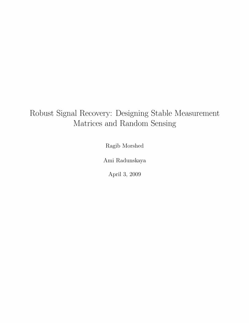
Abstract

In recent years a series of papers have developed a collection of results and theories showingthat it is possible to reconstruct a signal f ∈ Rn from a limited number of linear mea-surements of f . This broad collection of results form the basis of the intriguing theory ofcompressive sensing, and has far reaching implications in areas of medical imaging, compres-sion, coding theory, and wireless sensor network technology. Suppose f is well approximatedby a linear combination of m vectors taken from a known basis ψ. Given we know nothingin advance about the signal, f can be reconstructed with high probability from some limitednonadaptive measurements. The reconstruction technique is concrete and involves solving asimple convex optimization problem.

In this paper, we look at the problem of designing sensing or measurements matrices.We explore a number of properties that such matrices need to hold. We prove that oneof these properties in an NP-Complete problem, and give an approximation algorithm forestimating that property. We also discuss the relation of randomness and random matrixtheory to measurement matrices, develop a template based on eigenvalue distribution thatcan help determine random matrix ensembles that are suitable as measurement matrices,and look at deterministic techniques for designing measurement matrices. We prove thesuitability of a new random matrix ensemble using the template. We develop approaches toquantifying randomness in matrices using entropy, and a computational technique to identifygood measurement matrices. We also briefly discuss some of the more recent applications ofcompressive sensing.

Contents

1 Introduction 41.1 Nyquist-Shannon Theorem and Signal Processing . . . . . . . . . . . . . . . 41.2 Compressive Sensing: A Novel sampling/sensing Mechanism . . . . . . . . . 61.3 Summary . . . . . . . . . . . . . . . . . . . . . . . . . . . . . . . . . . . . . 6

2 Background 72.1 The Sensing Problem . . . . . . . . . . . . . . . . . . . . . . . . . . . . . . . 72.2 Sparsity and Compressible Signal . . . . . . . . . . . . . . . . . . . . . . . . 8

2.2.1 Transform Coding and its inefficiencies . . . . . . . . . . . . . . . . . 82.3 Incoherence . . . . . . . . . . . . . . . . . . . . . . . . . . . . . . . . . . . . 92.4 What Compressive Sensing is trying to solve? . . . . . . . . . . . . . . . . . 102.5 Relation to Classical Linear Algebra . . . . . . . . . . . . . . . . . . . . . . . 102.6 l2 norm minimization . . . . . . . . . . . . . . . . . . . . . . . . . . . . . . . 112.7 l0 norm minimization . . . . . . . . . . . . . . . . . . . . . . . . . . . . . . . 122.8 Basis Pursuit . . . . . . . . . . . . . . . . . . . . . . . . . . . . . . . . . . . 122.9 Summary . . . . . . . . . . . . . . . . . . . . . . . . . . . . . . . . . . . . . 13

3 Signal recovery from incomplete measurements 14

4 Robust Compressive Sensing 15

5 Designing Measurement Matrices 165.1 Randomness in Sensing . . . . . . . . . . . . . . . . . . . . . . . . . . . . . . 165.2 Restricted Isometry Property (RIP) . . . . . . . . . . . . . . . . . . . . . . . 17

5.2.1 Statistical Determination of Suitability of Matrices . . . . . . . . . . 205.3 Uniform Uncertainty Principle (UUP) and Exact Reconstruction Principle

(ERP) . . . . . . . . . . . . . . . . . . . . . . . . . . . . . . . . . . . . . . . 215.4 Random Matrix Theory . . . . . . . . . . . . . . . . . . . . . . . . . . . . . 23

5.4.1 Gaussian ensemble . . . . . . . . . . . . . . . . . . . . . . . . . . . . 235.4.2 Laguerre ensemble . . . . . . . . . . . . . . . . . . . . . . . . . . . . 285.4.3 Jacobi ensemble . . . . . . . . . . . . . . . . . . . . . . . . . . . . . . 29

5.5 Deterministic Measurement Matrices . . . . . . . . . . . . . . . . . . . . . . 295.6 Measurement of Randomness . . . . . . . . . . . . . . . . . . . . . . . . . . 31

1

5.6.1 Entropy Approach . . . . . . . . . . . . . . . . . . . . . . . . . . . . 315.6.2 Computational Approach . . . . . . . . . . . . . . . . . . . . . . . . . 33

5.7 Summary . . . . . . . . . . . . . . . . . . . . . . . . . . . . . . . . . . . . . 34

6 Applications of Compressive Sensing 35

7 Conclusion 36

2

List of Figures

1.1 How Shannon’s theorem is used? . . . . . . . . . . . . . . . . . . . . . . . . 5

2.1 Example of sparsity in digital images. The expansion of the image on a waveletbasis is shown to the right of the image. . . . . . . . . . . . . . . . . . . . . 9

2.2 l2 norm minimization. . . . . . . . . . . . . . . . . . . . . . . . . . . . . . . 112.3 l0 norm minimization . . . . . . . . . . . . . . . . . . . . . . . . . . . . . . . 122.4 l1 norm minimization . . . . . . . . . . . . . . . . . . . . . . . . . . . . . . . 13

5.1 Typical measurement matrix dimensions . . . . . . . . . . . . . . . . . . . . 185.2 Reduction using Independent Set. Vertex a and c form an independent set of

this graph. . . . . . . . . . . . . . . . . . . . . . . . . . . . . . . . . . . . . . 195.3 Statistical determination of Restricted Isometry Property [23] . . . . . . . . 215.4 Eigenvalue distribution of a Wishart matrix. Parameters: n=50, m=100 . . . 265.5 Eigenvalue distribution of a Manova matrix. Parameters: n=50, m1=100,

m2=100 (n×m1 and n×m2 are the dimensions of the matrix G forming thetwo Wishart matrices respectively) . . . . . . . . . . . . . . . . . . . . . . . 27

3

Chapter 1

Introduction

Signals are mathematical functions of independent variables that carry information. One canalso view signals as an electrical representation of time-varying or spatial-varying physicalquantities, the so called digital signal. Signal processing is the field that deals with theanalysis, interpretation, and manipulation of such signals. The signals of interest can beof the category of sound, video, images, biological signals such as in MRIs, wireless sensornetworks and others. Due to the myriad applications of signal processing systems in our dayto day life, it turns out to be an important field of research.

The concept of compression has also enabled us to store and transmit such signals inmany modern-day applications. For example, image compression algorithms help reducedata sets by orders of magnitude, enabling the advent of systems that can acquire extremelyhigh-resolution images [3]. Signals and compression are apparently interlinked, and thathas made it feasible to develop all sorts of modern-day innovations. In order to acquire theinformation in the signal, the signal needs to be sampled. Conventionally, sampling signalsis determined by Shannon’s celebrated theorem.

1.1 Nyquist-Shannon Theorem and Signal Processing

Theorem 1. Suppose f is a continuous-time signal whose highest frequency is less thanW/2, then

f(t) =∑

n∈Z f( nW

)sinc(Wt− n).

where sinc(x) = sin(πx)πx

.

f has a continuous Fourier transform and f( nW

) are the samples of f(t) taken at intervalsof n

W. We exactly reconstruct the signal f from its samples, weighted with shifted, scaled

sinc functions. We deal with the proof of this theorem later in the paper (proof outline isgiven in Appendix A). However, in essence, the theorem states that in order to reconstructa signal perfectly, the sampling rate must be at least twice the maximum frequency presentin the signal.

4

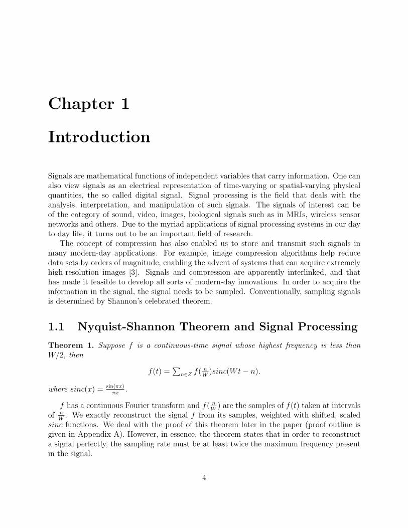
Figure 1.1: How Shannon’s theorem is used?

The example in Figure 1.1 will make Theorem 1 clearer. The curve is a Fourier transformof the signal that is to be sampled. According to Nyquist-Shannon theorem, in order toreconstruct the original signal (or its Fourier transform) perfectly, the signal needs to besampled at twice the maximum frequency present in the signal (the red dots in the figure inthis example).

This sampling frequency, W in this case, is known as the Nyquist rate, and underliesall signal acquisition protocols used in consumer electronics, radio receivers, and medicalimaging devices. Although, there are systems and devices that are not naturally bandlimited,but their construction usually involves using bandlimiting filters before sampling, and so isalso dictated by Shannon’s theorem [1].

The Nyquist rate turns out to be really high for a lot of cases leading to inefficiencies inthe protocol system. For example, in typical digital cameras, the millions of pixels take in alot of information about the environment, but then uses compression techniques to representthe information by storing only the important coefficients, after transformation of the signalinto an appropriate basis, and throwing away the rest of the insignificant coefficients. Thisespecially becomes a problem for MRI devices which are hardware limited [1]. For MRIdevices, in order to get a really good MRI image, a lot of samples are necessary, whichtranslates to keeping the patient in the MRI machine for a really long time. Compared totypical MRI times of maximum a few minutes, this would require having a patient in themachine for a few hours. For a lot of cases, this is practically impossible because of the costand time constraints involved.

However, it is possible to move away from the traditional method of signal acquisitiontowards more efficient methods. In fact, it might be possible to even build the compressionprocess into the acquisition process itself. In recent years, a novel theory of sensing/samplingparadigm has emerged known as compressive sensing or compressive sampling (CS) that canessentially solve this problem.

5

1.2 Compressive Sensing: A Novel sampling/sensing

Mechanism

Compressive sensing theory asserts that it is possible to recover certain signals from farfewer measurements or samples as dictated by the traditional theory. From an informationtheory point of view, this is equivalent to saying that given a few measurements about somedata, where it seems the measurements are not enough to accurately reconstruct the data,it might still be possible to reconstruct the data given certain structure exists in the data.An interesting aspect of compressive sampling is that it touches upon numerous fields inthe applied sciences and engineering such as statistics, information theory, coding theory,and theoretical computer science [4]. Currently, there are a number of research groupsworking on different applications of compressive sensing as well. For example, compressivesensing techniques have been used to develop a robust face recognition algorithm [15], andclassification of human action using wearable motion sensor network [16]. In this paper, welook in details of this new theory, specially focusing on designing measurement matrices forsignal acquisition.

1.3 Summary

In this section we looked at the traditional theory that guides almost all signal processingsystems (for a proof of the theorem see Appendix A). We looked at some of the problemsassociated with this theory when the measurement process is limited or very expensive. Apossible solution to this problem of reconstructing data from seemingly fewer measurementsthan necessary is addressed by the theory of Compressive Sensing. Compressive Sensingasserts that, under certain constraints, it is possible to reconstruct data from far fewermeasurements of the data than dictated by the the traditional theory.

6

Chapter 2

Background

Compressive sensing, also known as compressive sampling, emerged as a theory aroundthe year 2000, and exploded in the following years. Compressive sensing goes against theconventional wisdom of signal processing (Nyquist-Shannon Theorem) by stating that thisis inaccurate. Surprisingly, it is possible to reconstruct a signal (for example an image) quiteaccurately, or even exactly, from very few available samples compared to the original signaldimension. The novelty of compressive sensing lies in its underlying challenge to typicalsignal processing technique [4].

Before delving into the theory behind compressive sensing, one needs to understand thesensing problem itself from a mathematical perspective.

2.1 The Sensing Problem

The sensing problem is simply the question of how one can obtain information about a signalbefore any kind of ‘processing’ is applied on it. Throughout this paper, for all purposes of thesignal mechanisms described, information about a signal f(t) is obtained as linear functionalsrecording the values

yk = 〈f, φk〉 , k = 1, ...,m (2.1)

The idea is to establish a correlation between the object/signal one wants to acquire withsome sort of waveform, φk(t). For example, the sensing waveform(s), φ, can be the spikefunction. In that case, the resultant vector, y, is a vector of samples of f in either the timeor space domain. For a more applied perspective, the waveform(s) can be thought of as anindicator function of pixels; y is then the image data that is typically collected by sensors indigital cameras [1]. In this paper, we restrict ourselves to the discrete signal case, f ∈ Rn.The discrete case is simpler and the current theory of compressive sensing is far developedfor this case than the continuous - although the continuous case is pretty similar [1].

The theory of compressive sensing is built upon two very important concepts - spar-sity and incoherence. These two ideas form the fundamental premise that underlies all ofcompressive sensing.

7

2.2 Sparsity and Compressible Signal

The concept of Sparsity is not new in signal processing. A signal, f , is said to be sparse ifthe information in the signal can be represented using only a few non-zero coefficients whenthe signal is expanded on an orthonormal basis, ψ. More formally, f ∈ Rn (for example, a npixel image) is expanded in an orthonormal basis, such as wavelet basis, ψ = [ψ1, ψ2, ..., ψn]as follows [1]:

Definition 1 (Sparsity).

f(t) =n∑

i=1

xiψi(t) (2.2)

where x is the coefficient sequence of f, xi =< f, ψi >.The signal f is said to be S sparse if only S of the coefficients of x are non-zero. The

essential point here is that when a signal has sparse representation, one can discard the smallcoefficients without any significant loss of information in the signal.

Signals like f in the real world are not exactly sparse in any orthogonal basis. However,a common model termed compressible signals quite accurately approximate the nature ofsparse representation [6]. A compressible signal is such that the reordered entries of theψ expansion coefficients of f decay like a power law; i.e. if arranged in decreasing orderof magnitude, the nth largest entry obeys |xn| ≤ Const · n−s for some s ≤ 1. Ideas ofcompression are already in use in many typical compression algorithms (JPEG-2000) [2].

Another example of a typical sparse representation basis for signals is the commonlyknown Fourier basis, ψj(t) = n−

12 e

i2πjtn .

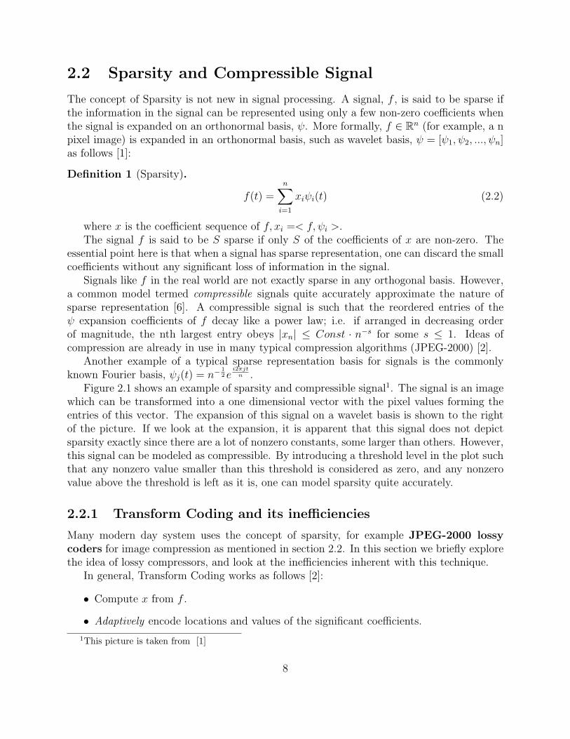
Figure 2.1 shows an example of sparsity and compressible signal1. The signal is an imagewhich can be transformed into a one dimensional vector with the pixel values forming theentries of this vector. The expansion of this signal on a wavelet basis is shown to the rightof the picture. If we look at the expansion, it is apparent that this signal does not depictsparsity exactly since there are a lot of nonzero constants, some larger than others. However,this signal can be modeled as compressible. By introducing a threshold level in the plot suchthat any nonzero value smaller than this threshold is considered as zero, and any nonzerovalue above the threshold is left as it is, one can model sparsity quite accurately.

2.2.1 Transform Coding and its inefficiencies

Many modern day system uses the concept of sparsity, for example JPEG-2000 lossycoders for image compression as mentioned in section 2.2. In this section we briefly explorethe idea of lossy compressors, and look at the inefficiencies inherent with this technique.

In general, Transform Coding works as follows [2]:

• Compute x from f .

• Adaptively encode locations and values of the significant coefficients.

1This picture is taken from [1]

8

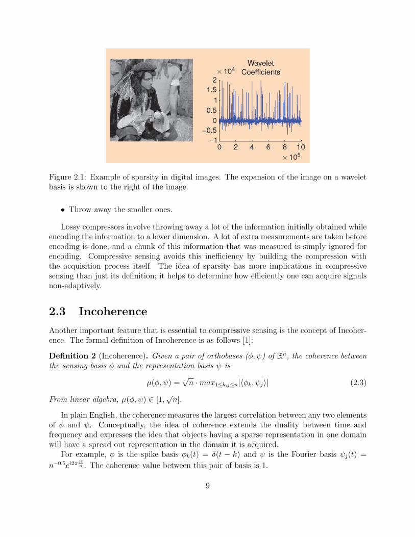
Figure 2.1: Example of sparsity in digital images. The expansion of the image on a waveletbasis is shown to the right of the image.

• Throw away the smaller ones.

Lossy compressors involve throwing away a lot of the information initially obtained whileencoding the information to a lower dimension. A lot of extra measurements are taken beforeencoding is done, and a chunk of this information that was measured is simply ignored forencoding. Compressive sensing avoids this inefficiency by building the compression withthe acquisition process itself. The idea of sparsity has more implications in compressivesensing than just its definition; it helps to determine how efficiently one can acquire signalsnon-adaptively.

2.3 Incoherence

Another important feature that is essential to compressive sensing is the concept of Incoher-ence. The formal definition of Incoherence is as follows [1]:

Definition 2 (Incoherence). Given a pair of orthobases (φ, ψ) of Rn, the coherence betweenthe sensing basis φ and the representation basis ψ is

µ(φ, ψ) =√n ·max1≤k,j≤n|〈φk, ψj〉| (2.3)

From linear algebra, µ(φ, ψ) ∈ [1,√n].

In plain English, the coherence measures the largest correlation between any two elementsof φ and ψ. Conceptually, the idea of coherence extends the duality between time andfrequency and expresses the idea that objects having a sparse representation in one domainwill have a spread out representation in the domain it is acquired.

For example, φ is the spike basis φk(t) = δ(t − k) and ψ is the Fourier basis ψj(t) =

n−0.5ei2π jtn . The coherence value between this pair of basis is 1.

9

In compressive sensing, we are interested in very low coherence pairs, i.e. the value ofcoherence is close to 1. Intuitively, this makes sense since the higher the incoherence betweenthe sensing and representation domain the lesser the number of coefficients necessary torepresent the information in the signal.

2.4 What Compressive Sensing is trying to solve?

Given a signal that has a sparse representation in any basis, compressive sensing theorytells us that it is possible to recover the sparse signal from a limited set of measurementsthan deemed by traditional signal processing. The formal definition of the problem thatcompressive sensing is trying to solve is articulated below:

Definition 3 (Compressive Sensing problem). Given a sparse signal x0 ∈ Rn whose sup-port T0 = t : x0(t) 6= 0 has small cardinality, and all we know about x0 are m linearmeasurements of the form

yk = 〈x0, ak〉, k = 1, ...,m or y = Ax0

where ak ∈ Rn are known test signals.

When this system is vastly underdetermined, m << n, can we recover the signal x0?

2.5 Relation to Classical Linear Algebra

Ideas from compressive sensing closely resounds with those in classical linear algebra. Theconcept of solving the system Ax = b, a most common problem in classical linear algebra, iswhat compressive sensing deals with as well. The sparse signal is represented as x, A beingthe measurement or sensing matrix that extracts the information from the signal x, and b isthe set of measurements which has a dimension far less than the dimension of x.

When the matrix A has more rows than columns, that is, the classical system is overde-termined, the exact solution x is recoverable. The number of rows correspond to the numberof constraints, and in an overdetermined system these constraints serve to reduce the dimen-sion or subspace where the solution can lie, eventually boiling down on the exact solutionx.

Compressive sensing is more interested with the second case: the matrix A has morecolumns than rows, that is, this classical system is underdetermined. According to theoryof linear algebra, such a system has infinitely many solutions to x, since each row, being aconstraint, only reduces the high dimension into lower dimensions (for example a line or aplane) where infinite solutions of x lie.

A best approximation can be determined classically using the idea of least squares solution(minimum l2 norm), or in other words a solution with the least energy. This technique givesa solution that satisfies the constraint of the systems most closely. For a lot of cases, thisleast square approximation solution is sufficient. However, when such a technique is applied

10

to for signal recovery in compressive sensing, this completely fails: the sparse signal cannotbe recovered. Compressive sensing takes advantage of the sparsity in the signal, and bytreating this as an additional constraint to the system Ax = b, enables recovery of the sparsesolution. There are new and efficient techniques that have been developed for compressivesensing which can solve the recovery problem efficiently. This is a huge difference that setsapart ideas from compressive sensing and classical linear algebra.

2.6 l2 norm minimization

From the previous section, l2 fails to recover the sparse solution x to the system Ax = b.The mathematical formulation for this minimization problem is given by equation(2.4).

x# = argmin||x||2 such that Ax = y (2.4)

Figure 2.2: l2 norm minimization.

Figure 2.2 shows why this fails. Assume that our space is two dimensional, and thesolution x lies on the lower dimensional subspace represented by the slanted straight line.The sparse solutions always lie on the coordinate axis. If we create an l2 ball, i.e. a circle,and expand it from the origin, the point of intersection of the l2 ball with the subspace wherex lies is the best approximation that is obtained. Clearly, as we can see from figure 1, thissolution is incorrect.

11

2.7 l0 norm minimization

Failure of l2 norm minimization demands the need for other techniques. For example, the l0norm minimization as shown in equation(2.5).

x# = argmin||x||0 such that Ax = y where ||x||0 = maxn|xi| (2.5)

The l0 norm is a less frequently used norm, but the idea is very simple. It is written as||x||0 = maxn|xi|. That is, it checks for presence of non-zero components in the sparse signalx.

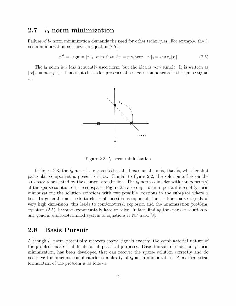
Figure 2.3: l0 norm minimization

In figure 2.3, the l0 norm is represented as the boxes on the axis, that is, whether thatparticular component is present or not. Similar to figure 2.2, the solution x lies on thesubspace represented by the slanted straight line. The l0 norm coincides with component(s)of the sparse solution on the subspace. Figure 2.3 also depicts an important idea of l0 normminimization; the solution coincides with two possible locations in the subspace where xlies. In general, one needs to check all possible components for x. For sparse signals ofvery high dimension, this leads to combinatorial explosion and the minimization problem,equation (2.5), becomes exponentially hard to solve. In fact, finding the sparsest solution toany general underdetermined system of equations is NP-hard [8].

2.8 Basis Pursuit

Although l0 norm potentially recovers sparse signals exactly, the combinatorial nature ofthe problem makes it difficult for all practical purposes. Basis Pursuit method, or l1 normminimization, has been developed that can recover the sparse solution correctly and donot have the inherent combinatorial complexity of l0 norm minimization. A mathematicalformulation of the problem is as follows:

12

x# = argmin||x||1 such that Ax = y (2.6)

Figure 2.4: l1 norm minimization

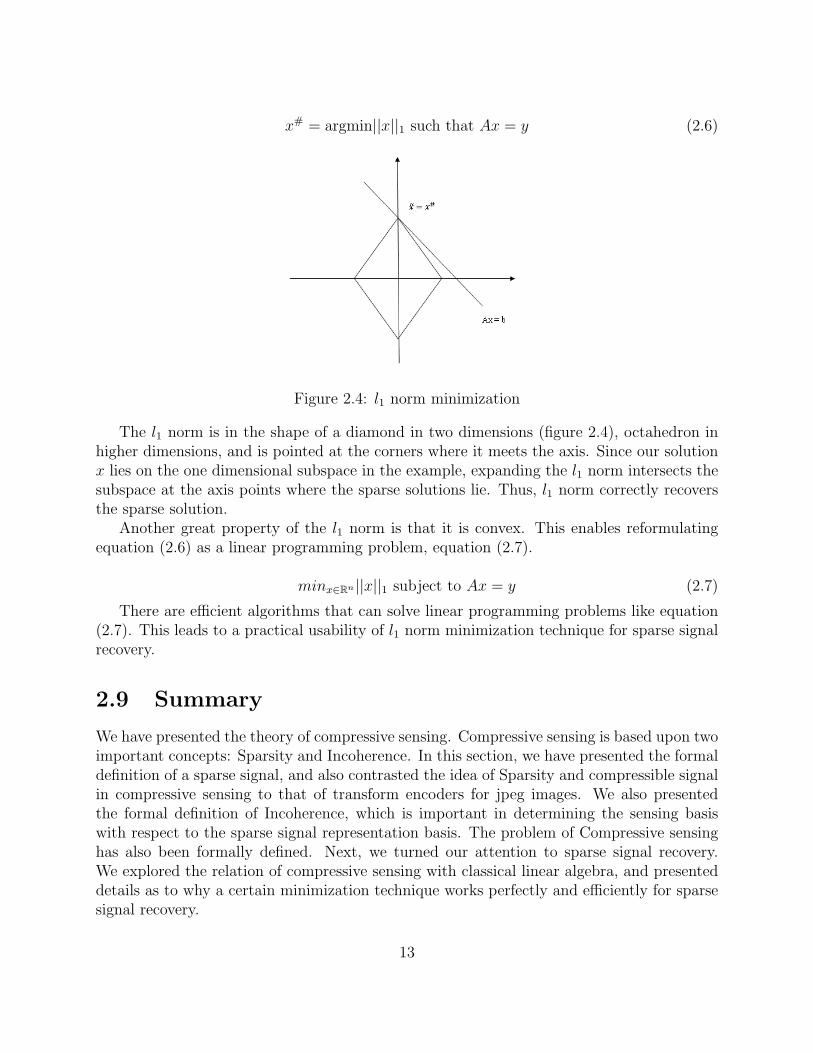
The l1 norm is in the shape of a diamond in two dimensions (figure 2.4), octahedron inhigher dimensions, and is pointed at the corners where it meets the axis. Since our solutionx lies on the one dimensional subspace in the example, expanding the l1 norm intersects thesubspace at the axis points where the sparse solutions lie. Thus, l1 norm correctly recoversthe sparse solution.

Another great property of the l1 norm is that it is convex. This enables reformulatingequation (2.6) as a linear programming problem, equation (2.7).

minx∈Rn||x||1 subject to Ax = y (2.7)

There are efficient algorithms that can solve linear programming problems like equation(2.7). This leads to a practical usability of l1 norm minimization technique for sparse signalrecovery.

2.9 Summary

We have presented the theory of compressive sensing. Compressive sensing is based upon twoimportant concepts: Sparsity and Incoherence. In this section, we have presented the formaldefinition of a sparse signal, and also contrasted the idea of Sparsity and compressible signalin compressive sensing to that of transform encoders for jpeg images. We also presentedthe formal definition of Incoherence, which is important in determining the sensing basiswith respect to the sparse signal representation basis. The problem of Compressive sensinghas also been formally defined. Next, we turned our attention to sparse signal recovery.We explored the relation of compressive sensing with classical linear algebra, and presenteddetails as to why a certain minimization technique works perfectly and efficiently for sparsesignal recovery.

13

Chapter 3

Signal recovery from incompletemeasurements

Sparse signal recovery is an important area in compressive sensing where a lot of workhas been done, and is currently an area of research. The basic idea of signal recovery isrelated to what we have seen in the previous sections using different norm minimizations,but work is being done on refinements of these techniques and more efficient algorithms.The l1 norm minimization is well established in the paper by Donoho [8]. Donoho alsoshowed that heuristic techniques to recover sparse solutions, for example, greedy algorithmsand thresholding methods, perform inadequately in recovering sparse solutions. Candes,Romberg and Tao in [14] addresses issues to recovering data for both noiseless and noisyrecovery. They also relate recovery to the importance of well designed sensing matrices. Theidea of random projection and its relation with signal reconstruction is addressed by Candesand Romberg in [6]. In this paper, they also highlight the importance of random projection- we will look into details of effectiveness of randomness as a sensing mechanism in a laterchapter - and discuss its implication in areas of data compression and medical imaging.

14

Chapter 4

Robust Compressive Sensing

In reality, signals do not have an exact sparse representation. Such signals are modeled ascompressive signals (see Sparsity), with a threshold such that any values above the thresholdare considered non-zeros and values below are treated as zeros. This approximates the spar-sity model. Signals also have inherent noise, in the form of measurement noise or instrumentnoise. For example, when a signal is sent as packets over the Internet, a lot of these pack-ets might get lost or corrupted. Given the signal has a sparse representation, compressivesensing asserts that the original signal is still recoverable. Any small perturbation in theobserved signal will induce small perturbation in the reconstruction [4]. In this case, themeasurements are modeled as

y = Ax+ e (4.1)

The vector e is a vector of errors or measurement noise. e can be either stochastic ordeterministic with a maximum total bound, i.e. ||e||l2 ≤ ε. The sparse signal can still berecovered, within its error bounds, by solving the l1 minimization problem, equation (4.2).

minx∈Rn||x||1 subject to Ax− y ≤ ε (4.2)

In this case, the reconstruction is consistent within the noise level present in the data.We expect that Ax− y is within the noise level of the data since clearly we cannot do betterthan this with the inherent noise. For this paper, we only consider the simplified case wherethere is no noise in the signal measurements. However, the ideas we discuss in the paper caneasily be extended for the case of signals with noise.

15

Chapter 5

Designing Measurement Matrices

Measurement matrix design is an important problem in compressive sensing. It is also adifficult problem. Designing a good measurement matrix is important since data recovery isdependent on how well the limited measurements provide information about the structureof the signal. An inherent quality of a good measurement matrix is that it should ensurethat there is enough ‘mixing’ of the information from the original signal in the limitedmeasurements. In other words, there should be enough representative information of theoriginal signal in the limited set of measurements.

5.1 Randomness in Sensing

Randomness of measurement matrices turns out to be an important aspect in signal mea-surements. This property ensures that the information represented by the limited set ofmeasurements is somewhat representative of the total information present in the originalsignal. Random matrices are largely incoherent with any fixed basis ψ ∈ Rn. This isimportant because, as we have seen previously, incoherent pairs determine the number ofmeasurements necessary for any signal. Presence of high randomness in a measurement ma-trix makes it suitable for use as a sensing matrix with any representation basis. In otherwords, this can serve as an universal measurement matrix.

Candes and Romberg [5] have shown that for exact reconstruction with high probability,only m random measurements uniformly chosen from the φ domain are needed,

m ≥ C · µ2(φ, ψ) · S · log n (5.1)

where C is a positive constant, µ is the incoherence value, and S is the number of nonzerocomponents in the sparse signal x.

Theorem 2. [5] Let f ∈ Rn and suppose x is the coefficient expansion of f in the basis ψand is S-sparse. Choose a subset Ω of the measurement domain of size |Ω| = m, and let mbe selected in the φ domain uniformly at random. Then if

m ≥ C · µ2(φ, ψ) · S · log n (5.2)

16

for some positive constant C, then the sparse signal can be recovered exactly from equation(2.7), i.e. l1 minimization, with overwhelming probability.

In [5], a detailed proof of this theorem is given and it is also shown that the probabilityof success of exact reconstruction exceeds 1− δ if m ≥ C · µ2(φ, ψ) · S · log(n/δ).

It is interesting to note a few things here. If the two basis are highly incoherent (µ isclose to 1) then only a few samples are needed. There is no information loss by measuringonly just about any set of m coefficients, and it may be far less than the signal size; if µ(φ, ψ)is very close to 1, only S log n measurements are sufficient for exact reconstruction. Thisis also a minimum bound and we cannot do with any lesser number of samples than this.Also, in order to do the reconstruction using equation (2.7), no previous knowledge aboutthe number of nonzero coordinates of x, their locations, or their amplitudes is needed [1].This also implies that the measurement basis can serve as an encoding system for signals.

In order to reconstruct a signal at least as good as fS, where fS is the representation ofthe original signal using only the S largest coefficient of the expansion of f , one only needsmeasurements of the order of O(S log(n/S)) [1].

5.2 Restricted Isometry Property (RIP)

In order to determine how good any given matrix is as a sensing matrix, it has to satisfy theRestricted Isometry Property (RIP). However, first we need to define the ‘Isometry constant’.

Definition 4 (Isometry constant). For each integer s = 1,2,..., define the Isometry constantδS of a matrix A as the smallest number such that

(1− δS)||x||2l2 ≤ ||Ax||2l2 ≤ (1 + δS)||x||2l2 (5.3)

hold for all S-sparse vectors x.

A given matrix A satisfies RIP if δS is not too close to 1. If it is close to 1, then theequation is trivial to define. Candes and Walkin [1] proved that for δS <

√(2) − 1, the

solution to the reconstruction is exact with high probability if the measurements are takenby the matrix satisfying this δS value for any signal. There is also an important theoremrelating δS and signal recovery.

Theorem 3. [12] (Noiseless recovery) Assume that δ2S ≤√

(2)− 1. Then the solution x∗

to the l1-norm minimization obeys

||x∗ − x||l1 ≤ C0||x− xS||l1 (5.4)

and||x∗ − x||l2 ≤ C0s

−1/2||x− xS||l1 (5.5)

where C0 is some constant. xS is defined a s the vector x with all but the S-largest entriesset to zero.

17

Two important assertions emerge from this theorem.

• If δ2S ≤ 1 the l0 problem has a unique S-sparse solution.

• If δ2S ≤√

(2)−1 then the solution given by the l1 minimization is exactly the solutiongiven by the l0 minimization; the convex relaxation problem is exact.

[12] has more details regarding the proof of Theorem 3.Restricted Isometry Property (RIP) is an elegant way to determine whether any arbitrary

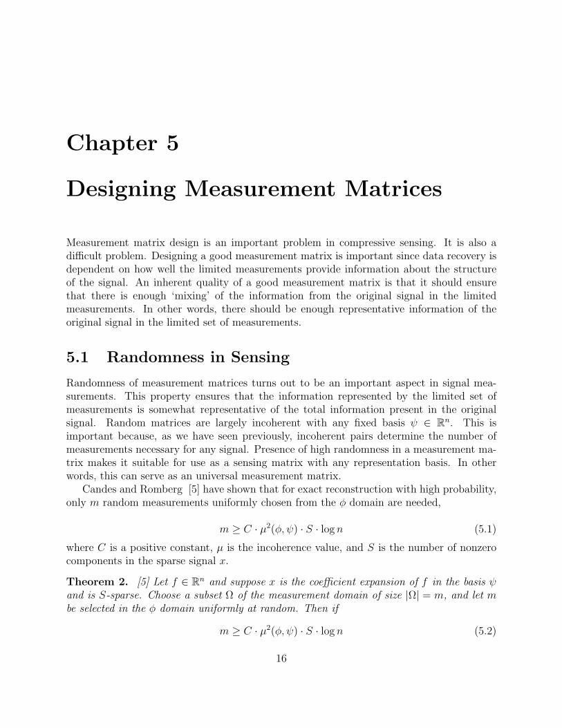
matrix is suitable as a sensing matrix. In our case the measurement matrices are short andfat (figure 5.1). Since the limited measurements we take are linear combinations of somecolumns of the matrix A, linear independence somehow has to be preserved in these matrices.Restricted Isometry Property (RIP) ensures that there are some subset of columns of the

Figure 5.1: Typical measurement matrix dimensions

matrix that are linearly independent/orthogonal. Specifically, any size S subsets of arbitrarycolumns of matrix A is nearly orthogonal.

It seems like one can take an infinite number of matrices of some particular dimensionsand try to prove the Restricted Isometry Property (RIP) for each matrix. In this way, thematrices that satisfy the property can be classified as belonging to the set of matrices suitablefor sensing purposes. However, there is an inherent problem with this idea. Firstly, one hasto start with a large set of matrices which can be difficult to obtain, but the major problemlies in determining Restricted Isometry Property (RIP) for each matrix.

In fact, proving Restricted Isometry Property (RIP) for any matrix means one has tocheck for all size S subsets of the columns of the matrix for near orthogonality. This mightbe harder than it seems. For a given set of subsets of the columns of the matrix, it is easyto test for orthogonality of these set of columns. We claim that the problem of determiningRestricted Isometry Property (RIP) is in Non-deterministic Polynomial Complete (NPC).

Lemma 1. Restricted Isometry Property (RIP) is NP-Complete.

Proof. Let A be the given matrix with cis the columns of A. That is, A = [c1, c2, ..., cm].Define some subset, P , of columns of A such that |P | = S, where S is the sparsity of thesignal. A holds RIP if there is a set P such that ∀i, j in the index set of P , cicj = 0(the columns in this set are mutually orthogonal). We can define the Restricted IsometryProperty problem as a formal language (Sparse Orthogonal Vector):

SOV = < A, S >: A has a subset of size S consisting of some columns from A such thatthe columns are mutually orthogonal.

18

We now want to show what SOV is in NP. In order to do that, we show that given acertificate consisting of a subset of columns of A, it is easy to verify in polynomial timewhether this set of columns are orthogonal. This can be done by checking orthogonality foreach pair of column vectors in the subset, and all these operations can be done in polynomialtime. Thus, SOV ∈ NP.

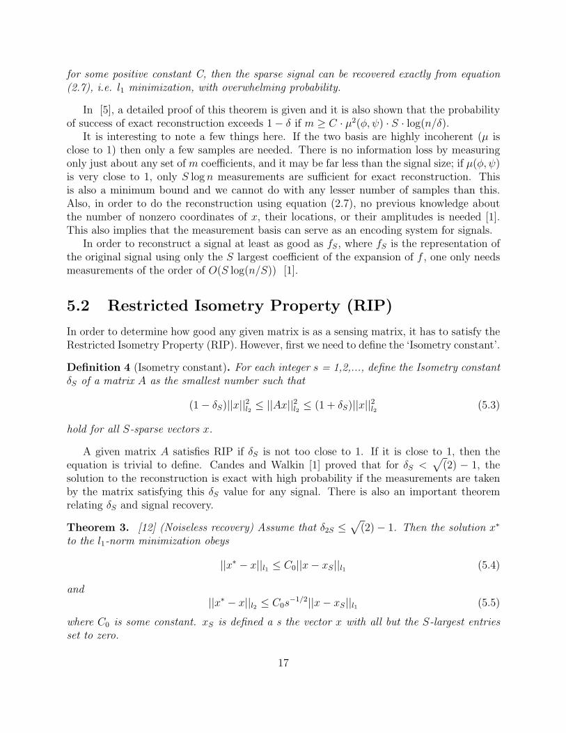
Now, we choose a known NPC problem Independent Set to reduce it down to SOV. TheIndependent Set problem is defined as follows:IS = < G,S >: Graph G has an independent set of size S.We want to show that IS≤pSOV.Label the edges with unique integers and create the matrix A = [c1, c2, ..., cm] where m equalsthe number of vertices in the vertex set of G, and the number of rows of each column vectorequal the size of the edge set of G.

For each vertex of column, the entry is 1 if vi is incident to edge ej. For independent setsof G, the entries of the columns are not in the same location in the vector since there are noincident edges common between these vertices. This reduction can be done in polynomialtime by looking through the set of vertices and checking the incident edges on the vertices.

Figure 5.2: Reduction using Independent Set. Vertex a and c form an independent set ofthis graph.

Thus, a maximally independent set of size S corresponds to the subset of size S ofmutually orthogonal columns from A.

To show that a ‘yes’ in IS implies a ‘yes’ in SOV. For the vertices forming IS, the columns(by construction) are mutually orthogonal and the size of the subset of A is of size S as well.

To show that a ‘yes’ in SOV implies a ‘yes’ in IS. For some subset of size S of columns,

19

each column of this subset is mutually orthogonal to each other, that is, there are no 1 entriesin the same location for any column pair from this subset of columns. This translates tovertices of G that do not have any incident edges common In other words, an independentset of size S.

Hence, SOV is NP-Complete.

Thus by Lemma 1, we have shown that the Restricted Isometry Property (RIP) is NPC.For any given matrix, it becomes exponentially harder (in the size of the matrix) to verifysatisfiability of RIP. Also, any polynomial time solution to RIP will solve the famous P=NPproblem.

5.2.1 Statistical Determination of Suitability of Matrices

Even though exact determination of Restricted Isometry Property (RIP) is difficult, beingable to have some idea whether a matrix satisfies this property can have practical significance.Instead of checking for each size S subsets of the columns of the given matrix for nearorthogonality, it might be efficient if it is possible to statistically determine for any matrixhow closely it satisfies Restricted Isometry Property (RIP). We were motivated by [23] toprovide an algorithmic approach to statistically determining Restricted Isometry Property.The algorithm is polynomial time, and can be regarded as an approximation algorithm todetermining Restricted Isometry Property (RIP). The pseudo code is given as follows.

1. Pick a base random matrix generation process: Gaussian, Binary or Fourier.

2. For t = θTMθM , and for every value 1 to M , and for chosen base process

• Generate sets M uniformly randomly over all sets, and scale each col-umn to unit norm.

• Calculate max and min eigenvalues.

3. Repeat step 2 for k samples of eigenvalues.

4. Calculate the mean and std. deviation of the max and min eigenvalues, foreach M .

5. Plot max and min eigenvalue vs Sparsity M.

Figure 5.3 shows an example of how the extremal eigenvalues of a matrix satisfyingapproximate-RIP compare to the extremal eigenvalue distribution of a known, base matrixthat satisfies RIP. For this particular example, the green curve (dotted line) corresponds tothe base Gaussian matrix, and the blue curve (solid line) corresponds to a test matrix.

20

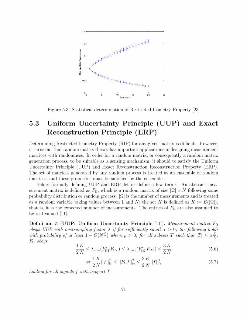
Figure 5.3: Statistical determination of Restricted Isometry Property [23]

5.3 Uniform Uncertainty Principle (UUP) and Exact

Reconstruction Principle (ERP)

Determining Restricted Isometry Property (RIP) for any given matrix is difficult. However,it turns out that random matrix theory has important applications in designing measurementmatrices with randomness. In order for a random matrix, or consequently a random matrixgeneration process, to be suitable as a sensing mechanism, it should to satisfy the UniformUncertainty Principle (UUP) and Exact Reconstruction Reconstruction Property (ERP).The set of matrices generated by any random process is treated as an ensemble of randommatrices, and these properties must be satisfied by the ensemble.

Before formally defining UUP and ERP, let us define a few terms. An abstract mea-surement matrix is defined as FΩ, which is a random matrix of size |Ω| ×N following someprobability distribution or random process. |Ω| is the number of measurements and is treatedas a random variable taking values between 1 and N ; the set K is defined as K := E(|Ω|),that is, it is the expected number of measurements. The entries of FΩ are also assumed tobe real valued [11].

Definition 5 (UUP: Uniform Uncertainty Principle [11]). Measurement matrix FΩ

obeys UUP with oversampling factor λ if for sufficiently small α > 0, the following holdswith probability of at least 1 − O(N

ρα ) where ρ > 0, for all subsets T such that |T | ≤ αK

λ.

FΩ obeys1

2

K

N≤ λmin(F ∗ΩTFΩT ) ≤ λmax(F

∗ΩTFΩT ) ≤ 3

2

K

N(5.6)

⇔ 1

2

K

N||f ||2l2 ≤ ||FΩf ||2l2 ≤

3

2

K

N||f ||2l2 (5.7)

holding for all signals f with support T .

21

In essence, Uniform Uncertainty Principle (UUP) is a definition about the maximum andminimum eigenvalue distribution of the matrices. The constants 1

2and 3

2are inconsequen-

tial in equation (5.6). It simply gives concreteness to the definition of UUP. However, theimportant aspect of the definition is the bounded nature of the minimum and maximumeigenvalues of the measurement matrix.

Uniform Uncertainty Principle (UUP) is similar in nature to many other different prin-ciples and results related to random projection. For example, Restricted Isometry Property(RIP) is similar to Uniform Uncertainty Principle (UUP). Although, the definitions of theseare not apparently similar at all, however, both are conceptually similar. For matrices thatsatisfy Restricted Isometry Property (RIP), column vectors picked from arbitrary subsetsof the set of columns of the measurement matrix are nearly orthogonal. The larger thesesubsets the better is the measurement matrix. In essence, randomness of matrices ensuresthat this property holds [1]. Random matrices also satisfy Uniform Uncertainty Principle(UUP). In other words, the distribution of the eigenvalues of measurement matrices seemsto have some relation with the near orthogonality of column vectors taken from arbitrarysubsets. This apparent duality might also have interesting consequences since Uniform Un-certainty Principle (UUP) can come to the rescue in cases where determining RestrictedIsometry Property (RIP) exactly might be difficult. Random matrices are one such examplesince it is natural to look at random matrices using the idea of an ‘abstract measurementmatrix’, rather than trying to determine Restricted Isometry Property (RIP) exactly.

Uniform Uncertainly Principle (UUP) is the crux in proving whether a random matrixensemble is suitable as a sensing matrix. If an ensemble satisfies UUP, and a matrix fromthis ensemble is used for taking measurements about some data, the original sparse signalcan be reconstructed using equation (2.7) with high probability.

However, there is second principle or hypothesis that is described by Candes and Tao in[11]. The principle is defined as follows:

Definition 6 (ERP: Exact Reconstruction Principle [11]). Measurement matrix FΩ

obeys ERP with oversampling factor λ if for all sufficiently small α > 0, each fixed subsetT obeying |T | ≤ αK

λ, and each ‘sign’ vector σ defined on T , |σ| = 1, there exists with

overwhelmingly large probability a vector P ∈ RN with the following properties:

1. P (T ) = σ(t),∀t ∈ T ;

2. P is a linear combination of the rows of FΩ, that is, P = F ∗ΩV for some vector V oflength |Ω|;

3. and |P (t)| ≤ 12∀t ∈ TC = 0, ..., N − 1\T .

‘Overwhelmingly large’ means that the probability is at least 1−O(Nρ/α for some fixed positiveconstant ρ > 0.

Exact Reconstruction Principle (ERP) is crucial in determining whether the recon-structed signal, x∗, is close to the original sparse signal, x, in the l1 norm. Both the ExactReconstruction Property (ERP) and Uniform Uncertainty Property (UUP) hypothesis are

22

closely related. We only concern ourselves with UUP in trying to determine whether arandom matrix ensemble is suitable as a sensing matrix because of the implication of theform,

UUP ⇒ ERP

for any signal x [11].In order to prove Uniform Uncertainty Principle (UUP) for any random matrix ensemble,

using the definition, one only needs to look for ensembles where the maximum and minimumeigenvalues of its matrices are bounded; that is, a distribution plot of the eigenvalues donot tail off to infinity. An abstraction for proving Uniform Uncertainty Principle (UUP)by studying the proofs from paper by Candes and Tao [11] is given as follows (note thatthis abstraction relies on known results on distribution of the singular values for the randommatrix ensemble of interest):

For X∗X or the singular values of X

1. The eigenvalues have a bounded distribution, i.e. the distribution do nottail off to infinity.

2. There exists some inequalities on the probabilistic bounds (exponential forsome known results) on the distance of the largest and smallest eigenvaluesfrom the median.

3. UUP is satisfied if the above two conditions hold.

5.4 Random Matrix Theory

There are three known random matrix ensembles that hold the Uniform Uncertainty Principle(UUP) [11]. These three ensembles are the Gaussian ensemble, Binary ensemble and Fourierensemble. The abstraction described in the previous section is based on studying UUP proofsof these ensembles, and extracting out the most important aspects of the proofs necessaryfor analyzing other random matrix ensembles. In this section we briefly present the proofoutline for one of these known ensembles in order to show how such a proof would follow.

5.4.1 Gaussian ensemble

Lemma 2 ( [11]). The Gaussian ensemble obeys the uniform uncertainty principle (UUP)with oversampling factor λ = logN .

Proof. Let X be an n by m matrix with n ≤ m, and with i.i.d. entries sampled from thenormal distribution with mean zero and variance 1

m. According to our proof abstraction, we

are interested in the singular of X, that is, the eigenvalues of X∗X.

23

There are known results about the eigenvalues of X∗X, and one such result states thatthe eigenvalues have a deterministic limit distribution supported on the interval[(1−

√c)2, (1 +

√c)2] as m,n→∞, with m/n→ c < 1. In [11], a known result about the

concentration of the extreme singular values for the Gaussian matrix is used.

P (λm(X) > 1 +√m/n+ r) ≤ e−nr2/2 (5.8)

P (λ1(X) < 1−√m/n− r) ≥ e−nr2/2 (5.9)

Now the remaining part is to prove that Gaussian ensemble obeys the UUP, and determinethe oversampling factor λ = logN .

To do that, fix K ≥ logN and let Ω := 1, ..., K. Let T be a fixed index set. The eventET is defined as

ET := λmin(F ∗ΩT ) < K/2N ∪ λmax(F∗ΩT ) > 3K/2N

Now, adding equation (5.8) and (5.9), and replacing n = K and r2/2 = c, it is possibleto write

P (ET ) ≤ 2e−cK

.Candes and Tao then looks at the tightness of the spectrum over all sets T ∈ Tm :=

|T | ≤ m where it is assumed that m is less than N/2.

P (∪TmET ) ≤ 2e−cK · |Tm| = 2e−cK ·m∑

k=1

(N

k

)≤ 2e−cK ·m

(N

m

)A known result

m∑k=1

(N

k

)≤ m

(N

m

)and

(Nm

)≤ eNH(m/N), where H is the binary entropy function, is used.

H(q) := −q log q − (1− q) log(1− q)

From the binary entropy function1, the inequality −(1 − q) log(1 − q) ≤ q holds since0 < q < 1.

Now, using the above

P (∪TmET ) ≤ 2e−cK ·m(N

m

)(5.10)

≤ 2e−cKmeNH(m/N) (5.11)

≤ 2e−cKmeN(−(m/N) log(m/N)−(1−(M/N)) log(1−(m/N))) (5.12)

≤ 2e−cKme−m log m+m log N+m (5.13)

≤ 2e−cKmem log(N/m)+m (5.14)

≤ 2e−cKelog mem log(N/m)+m (5.15)

≤ 2e−cKem log(N/m)+m+log m (5.16)

1Note that this is natural log

24

Equation (22) holds since −(1−m/N) log(1−m/N) ≤ (m/N).Taking log of equation(25),

log(P (∪TmET )) ≤ log 2− cK +m log(N/m) +m+ logm

≤ log 2− cK +m(log(N/m) + 1 +m−1 logm)

≤ log 2− ρK

given thatm(log(N/m)+1+m−1 logm) ≤ (c−ρK) which implies that−cK+m(log(N/m)+1 +m−1 logm) ≤ −ρK.

Thus, the Gaussian ensemble satisfies UUP with oversampling factor proportional toλ = log(N/K).

Details of this proof can be found in [11].

The proof is similar for the Binary ensemble and the Fourier ensemble. Although, for theFourier ensemble case, the bounded nature of the eigenvalue distribution is obtained usingideas of entropy. However, in general, once a known result about the concentration of thelargest and smallest eigenvalue of a random matrix ensemble is known, the proof basicallyfollows a template.

For this paper, we are interested in other random matrix ensembles apart from the threedescribed above. So far we have been able to identify two more potential random matrixensembles.

• Wishart Matrix (or Laguerre Ensemble):Let G be a N×M random matrix with independent, zero mean, unit variance elements.

W =1

MGG∗

The entries of G are i.i.d. normally distributed elements.

• Manova Matrix (or Jacobi Ensemble):The Manova matrix, J , is defined in terms of two Wishart matrices, W (c1) and W (c2)as

J = (W (c1) +W (c2))−1W (c1)

where c1 = NM1

, c2 = NM2

, and N ×M1,N ×M2 are dimensions of matrix G forming theWishart matrices.

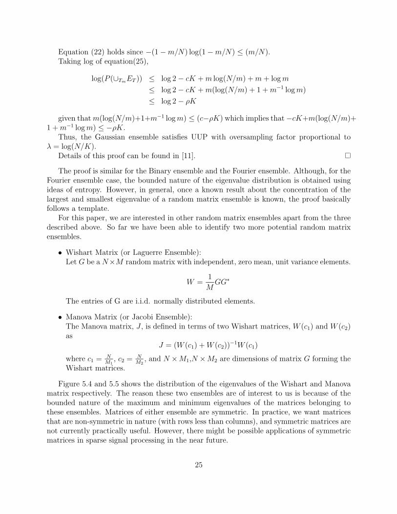
Figure 5.4 and 5.5 shows the distribution of the eigenvalues of the Wishart and Manovamatrix respectively. The reason these two ensembles are of interest to us is because of thebounded nature of the maximum and minimum eigenvalues of the matrices belonging tothese ensembles. Matrices of either ensemble are symmetric. In practice, we want matricesthat are non-symmetric in nature (with rows less than columns), and symmetric matrices arenot currently practically useful. However, there might be possible applications of symmetricmatrices in sparse signal processing in the near future.

25

Figure 5.4: Eigenvalue distribution of a Wishart matrix. Parameters: n=50, m=100

26

Figure 5.5: Eigenvalue distribution of a Manova matrix. Parameters: n=50, m1=100,m2=100 (n×m1 and n×m2 are the dimensions of the matrix G forming the two Wishartmatrices respectively)

27

Apart from these two, it would be interesting to figure out UUP for other random matrixensembles. This can be achieved by looking at the distribution of the singular values ofmatrices of the ensemble, and using any known results on the concentration of the largestand smallest eigenvalue from the singular decomposition for these random matrices.

For the cases described above, the entries of the random matrix are picked from an i.i.d.normal distribution. Another aspect of the problem that might be of interest is forming arandom matrix with entries from a uniform distribution.

One technique of generating a sensing matrix from a uniform distribution is by formingthe sensing matrix A by sampling n column vectors uniformly at random on the unit sphereof Rm.

5.4.2 Laguerre ensemble

Matrices of the Laguerre ensemble are as follows:

W =1

MGG∗ where entries of G are from an i.i.d. normal distribution.

Note that matrices of this class are symmetric in nature.

Lemma 3. The Laguerre ensemble obeys the uniform uncertainty principle (UUP) withoversampling factor λ = logN .

Proof. Let’s look at the singular values of W ∗W .

W ∗W = (1

MGG∗)∗(

1

MGG∗)

=1

M2G∗GGG∗

=1

M2(GG∗)2

We know from [11] that the distribution of the maximum and minimum eigenvalues of G∗Gfollow this:

P (λM(X) > 1 +√M/N + r) ≤ e−Nr2/2

P (λ1(X) < 1−√M/N − r) ≤ e−Nr2/2

where λ1(X) ≤ λ2(X)... ≤ λM(X).Then, for W ∗W it is

P (λ2M(X) > (1 +

√M/N + r)2) ≤ e−Nr2

(5.17)

P (λ2M(X) > (1−

√M/N − r)2) ≤ e−Nr2

(5.18)

Now,ET := λmin(F ∗ΩT ) < aK/N ∪ λmax(F

∗ΩT ) > bK/N

28

where a, b are constants.Adding equation (5.17) and (5.18)

P (ET ) ≤ 2e−Nr2

= 2e−Kc

where c = r2 and K = N .The rest of the proof from here follows exactly the Gaussian ensemble proof. Thus, the

oversampling factor is λ = logN .

5.4.3 Jacobi ensemble

The Jacobi ensemble is composed of Wishart matrices as shown in a previous section. Inorder to prove UUP, we need to know how the composition of the Wishart matrices affectsthe distribution of the maximum and minimum eigenvalue. (W (c1) + W (c2))

−1 has a veryhigh upper bound, in the worst case, for the largest eigenvalue. If either W (c1) or W (c2) hasa small eigenvalue, then the upper bound on the eigenvalue of the inverse sum is very large.

||(W (c1) +W (c2))−1W (c1)|| ≤ ||1/(W (c1) +W (c2))|| · ||W (c1)||

However, since the Wishart matrices are generated from an i.i.d. distribution the upperbound might generally be significantly less than this worst case. Figure 5.5 shows that infact this is true. The histogram shows that it is statistically likely that, due to the generationtechnique used, the minimum and maximum eigenvalues have a more optimistic bound.

This makes proving UUP for Jacobi difficult since one has to rely on a statistical likelihoodbound of the maximum and minimum eigenvalues. Assuming the likelihood of the minimumeigenvalue greater than zero and the maximum less than some δ for δ > 0, we are trying tofigure out an expression for the probabilistic bounds under this assumption.

A further refinement of random matrix generation might be to pick entries resulting fromsome chaotic process, and check satisfiability of UUP for such matrices. In future work, thisinteresting connection between random matrices and chaotic systems should be explored.Deterministic matrices are discussed in the next section.

5.5 Deterministic Measurement Matrices

All matrices that are suitable as a sensing matrix seem to have some inherent randomnessassociated with them. However, Candes and Tao conjectures in [11] that the entries of thesesensing matrices do not have to be independent or Gaussian, but completely deterministicclasses of matrices obeying the Uniform Uncertainty Principle could be constructed.

One design of deterministic measurement matrix is using chirp sequences [23]. Theidea in deterministic design is to go back to the concept of linear combinations. Sincerecovering the sparse signal is finding out which small linear combinations of the columnsof the measurement matrix forms the vector of measurements, the measurement matrix can

29

be designed to facilitate this. In fact, this concept is essentially the same as the concept ofRestricted Isometry Property. In [23], the authors form the columns of the measurementmatrix using chirp signals. The algorithm for generating such deterministic matrices is alsogiven in the paper.

A chirp signal is defined as follows

vm,r(l) = αej2πml

K+ j2πrl2

K

where m, r ∈ ZK , m is the base frequency, r is the chirp rate, and K is length of signal. Ina length K signal, there are K2 possible pairs of m and r.

Let the measurement vector be y, indexed by l, and formed by linear combination ofsome chirp signal

y(l) = s1ej2πm1l

K+

j2πr1l2

K + s2ej2πm2l

K+

j2πr2l2

K + ...

= s1vm1,r1(l) + s2vm2,r2(l) + ...

Since the columns of the measurement matrix are formed using chirp signals, the coeffi-cients si form the sparse signal of interest.

Now, chirp rates can be recovered from y by looking at y(l)y(l+d) where the index (l+d)is taken 2riTmodK.

f(l) = y(l)y(l+T ) = |s1|2ej2πK

(m1T+r1T 2)ej2π(2r1lT )

K + |s2|2ej2πK

(m2T+r2T 2)ej2π(2r2lT )

K + cross termswhere the cross terms are the chirps, and T ∈ ZK , T 6= 0.

At the discrete frequencies 2riTmodK, f(l) has sinusoids. If K is a prime number, thenthere is a bijection between the chirp rates and FFT bins. The cross terms in the remainderof the signal have their energy spread across all FFT bins.

Now, when y consists of sufficiently few chirps (that is, x is sparse), taking FFT off(l) results in a spectrum with significant peaks at locations corresponding to 2riTmodK.The chirp rates can be extracted from these peaks. The signal, y(l), can be dechirped by

multiplying by e−j2πril2

K , converting the chirp rate ri to sinusoids. Once FFT is performed onthe resulting signal, the values of mi and si can be retrieved. The sparse signal can then bereconstructed.

The authors have proved Restricted Isometry Property (RIP) approximately, i.e. in astatistical sense, for the sensing matrix formed using chirp signals as its columns. See [23]for details.

There also exists explicit constructions of deterministic matrices whose entries are 0 or1. However, it has been shown in [13] that such explicitly constructed 0,1 matrices requiremore rows than O(S log(n/S)) to satisfy the Restricted Isometry Property (RIP), and suchmatrices cannot achieve good performance with respect to RIP. This is articulated in thefollowing theorem:

Theorem 4 ( [13]). Let A be an m × n 0,1-matrix that satisfies (S,D)-RIP. Then, m ≥min

k2

D4 ,n

D2

where (S,D)-RIP is defined as

c2||Ax||22 ≤ ||x||22 ≤ c2D2||Ax||22

30

.

In order to create a good 0,1 sensing matrix, the number of rows m has to satisfy theminimum condition as stated in the theorem. However, generation of such a matrix mightnot be practically efficient.

As we have already seen, Restricted Isometry Property (RIP) and Uniform UncertaintyProperty (UUP) are somewhat difficult to prove. There are deterministic methods of gener-ating matrices, for example from chaotic processes, but proving randomness for such systemsis hard. If we look at random matrix theory, we already know the randomness associated withthe process that is generating the matrices. This is one reason measurement matrices arelikely to have more prominent candidates in random matrix theory. Designing deterministicmeasurement matrices that satisfy the Uniform Uncertainty Property (UUP) or RestrictedIsometry Property (RIP) is still an open problem.

5.6 Measurement of Randomness

Apart from figuring out how to design good measurement matrices for compressive sensing,it would be convenient to have some ‘measurement’ of the amount of randomness exhib-ited by the matrices. As we have seen, presence of high randomness is a good feature formeasurement matrices. Measurement of randomness can be a measure of the ‘goodness’ ofa matrix as a sensing matrix. There are two ways to look at randomness measurement:entropy approach and computability approach.

5.6.1 Entropy Approach

A common quantitative approach to randomness is to quantify the ‘entropy’ of the sys-tem. One idea is to look at the eigenvalue distribution for these matrices and quantify therandomness using this ‘spread’ of the eigenvalues. Another option might be to look at theoversampling factor, λ from Uniform Uncertainty Principle (UUP). The idea of oversamplingfactor is from an equation from [11]

||f − f#||l2 ≤ C ·R · (λ/K)r (5.19)

where ||f ||l1 ≤ R, r := 1/m − 1/2, and C is some constant. The reconstruction error,||f − f#||l2||, depends on the oversampling factor involved.

For the Gaussian and Binary random matrix ensembles, λ = logN , and for the Fourierrandom matrix ensemble λ = (logN)6. Just looking at these values, it seems reconstructionerror is minimum for the Gaussian and Binary ensemble, and higher for the Fourier ensemble.From a practical point of view, this entropy based on the oversampling factor suggests thatthe Gaussian and Binary ensembles are equally good measurement matrix ensembles, andthe Fourier ensemble is worse compared to both.

Randomness can also be quantified by calculating the entropy of the system from theprobability distribution. In quantifying randomness of measurement matrices, one can imag-ine a Rm×n dimensional space where all m × n matrices of some ensemble reside. There is

31

a sense of distribution of these matrices in the higher dimensional space, and we want tocapture the randomness associated with each matrix in this distribution. Both the Gaussianand Binary measurement matrices are generated by taking entries from a Gaussian prob-ability distribution and a Bernoulli probability distribution respectively. Since the entriesof the matrices are chosen from the probability distributions, intuitively it seems as if theinherent randomness of the sensing matrices generated using these particular distributionsshould correspond to the amount of randomness within the probability distributions. Ingeneral, entropy is calculated as follows,

H =∑∀i

pi ln pi

where pi is the probability of each event occurring. For a continuous case, this becomes

H =

∫P (j) lnP (j)dj

for some event j.It can be shown that the entropy of each matrix in our Rm×n space is the sum of the

entropy associated with selecting each entry of the matrix. The entropy of the matrixincreases as more entries are selected. Since the matrices of interest to us are of size m× n,where m << n, the scaling factor is mn for entropy of the matrix as a whole.

The probability of an entry is the associated probability of each entry being selected froma particular distribution. For the Gaussian distribution, with mean zero, the pdf is given by

P (x) =1√σ2π

e−x2

2σ2

and the entropy isHgaussian = ln(σ

√2πe).

Assuming our measurement matrices are of size d ×m, where d is the number of mea-surements and m is the original signal dimension of size 32000 (from images used in 5.6.2for recognition problem [24]), then

Hgaussian = md ln(1√m

√2πe) = −120, 570d

For a Bernoulli distribution, the pdf is

P (k) =

(1− p) k = −1/

√m

p k = 1/√m

and the entropy measurement is

Hbinary = md×−(1− p) ln(1− p)− p ln(p) = −22, 180d

32

assuming that there is a 0.50 probability of selection of either value as entries of the Binarymeasurement matrix. This simple calculation shows that even though the oversamplingfactor for either of these matrices is the same, in fact, the amount of randomness for theGaussian ensemble is significantly more than for the Binary ensemble.

We have not yet quantified randomness for the two promising matrix ensembles we de-scribed earlier, the Laguerre and Jacobi ensembles.

5.6.2 Computational Approach

For our computational approach, we test out the suitability of a matrix by using it as a sensingmatrix in a particular object recognition problem. A baseline for the object recognitionproblem has been established using matrices from the Gaussian ensemble, which satisfyUniform Uncertainty Principle (UUP) and is an example of a good sensing matrix. Using thisas a benchmark, any random matrix from another ensemble can be used, and the recognitionrate compared to the benchmark to determine its effectiveness as a sensing matrix. Our codeis available as a matlab file.

Recognition test on the Binary ensemble The Binary ensemble has been proven tosatisfy Uniform Uncertainty Principle (UUP) by Candes and Tao in [11]. Sensing matricesof the binary ensemble have entries taking values in −1/

√n, 1/

√n where n is the original

size of the signal.Our recognition problem is an image based face recognition problem where the train-

ing and testing set are projected onto a lower dimensional space we call ‘feature space’,and recognition is performed on this lower dimensional space by using sparse recovery tech-niques [15].

For the baseline with the Gaussian ensemble using a feature space size of 30, the averagesuccessful recognition percentage obtained is 85.43 ± 0.64%. Using the Binary ensemble asthe sensing matrix, with the same feature space dimension, training and testing set, theaverage percentage successful classification is 83.97± 0.17%.

As discussed previously, sensing matrices with high randomness are good for sparse signalrecovery. Our results from the recognition problem suggests that the amount of randomnessin the Binary ensemble might be less compared to that in the Gaussian ensemble. Com-paring this result with the oversampling factor, the difference in the recognition rates is notsignificant to deter the usability of the Binary ensemble for practical purposes. The errorin sparse signal reconstruction is low for Gaussian ensemble in practice, as suggested bythe difference in recognition rates, in contrast to that suggested by equation (5.19). Thisalso supports the previous entropy estimation of the Gaussian and Binary ensemble wherematrices from the Gaussian ensemble had higher entropy compared to those from the Binaryensemble.

33

5.7 Summary

In this section we have looked at designing measurement matrices, our main area of interestfor this paper. We introduced the importance of a good measurement matrix, and discussedthe effectiveness of randomness as a design tool. In contrast to randomness, we have alsodiscussed issues related to designing a deterministic measurement matrix. Some of theimportant concepts related to designing measurement matrices such as Restricted IsometryProperty (RIP), Uniform Uncertainty Property (UUP) and Exact Reconstruction Property(ERP) are also discussed in this section. We have shown that Restricted Isometry Property isa difficult problem to solve, and we have proved its NP-Complete nature. We also suggestedan approximation algorithm, which has a polynomial time bound, for estimating RestrictedIsometry Property (RIP) for any given matrix. We also explored relation of random matrixtheory with measurement matrices. We have suggested a proof template for proving UniformUncertainty Principle (UUP) for any suitable random matrix ensemble. In order to quantifyrandomness of different measurement matrices, we suggested techniques based on an entropycalculation approach and a computational approach that involves a recognition algorithm.

34

Chapter 6

Applications of Compressive Sensing

In this section we briefly explore some of the applications of compressive sensing. Applica-tions of compressive sensing range from coding theory to facial recognition. One researchgroup has developed a single pixel based camera based on the ideas from compressive sensing[2]. Compressive sensing also looks promising in the field of wireless sensor networks sincecompressive sensing ideas help reduce the complexity of the end sensors that are deployed inthe field. The processing can be carried out at a remote site with adequate computationalpower, and signal reconstruction would still be overwhelmingly exact even if data sent from anumber of sensors get lost. In medical imaging devices such as Magnetic Resonance Imaging(MRI) [14], compressive sensing carry great promise in better image reconstruction. Morecurrent application of compressive sensing is in facial recognition and human action classifiersystem [15], [16] respectively. The design techniques explored in this paper for measurementmatrices are equally important and applicable in a lot of these applications.

35

Chapter 7

Conclusion

Compressive sensing is a new tool that makes measurement process efficient and results ingood data reconstruction given there is a certain structure to the data of interest. Beingable to design good measurement matrices is imperative to obtain good reconstruction ofthe data. Randomness is an effective tool in signal projection and reconstruction. We haveshown that the Restricted Isometry Property (RIP) is a difficult property to determine, andin fact, it is a NP-Complete problem. However, we suggested an approximation algorithm toestimate RIP. We developed techniques to quantify entropy of matrices of a random matrixensemble by looking at the entropy of the associated probability, as well as a recognitionalgorithm based technique to quantify randomness. Using our techniques, one can determineeffectiveness of potential matrices as sensing matrices. In this paper, we explored differenttechniques and issues related to generation and design of effective sensing matrices. We hopeour work will motivate people to further look into relations between sensing matrices andrandom (or even chaotic) processes.

36

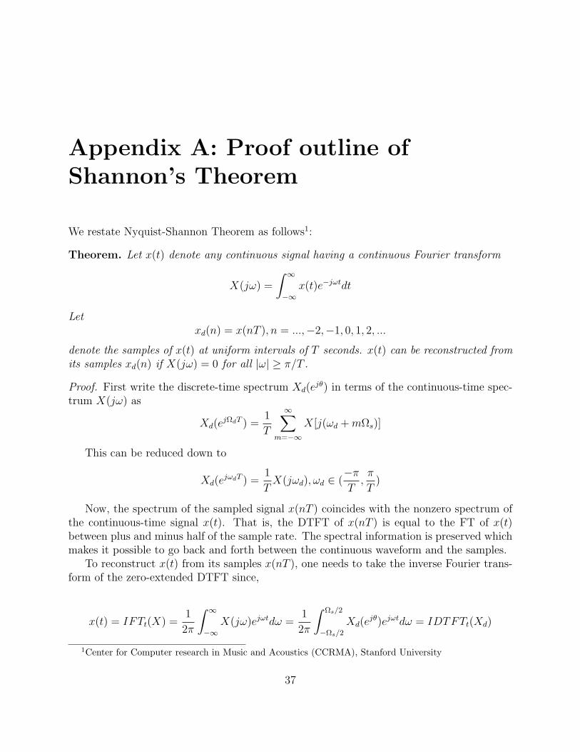
Appendix A: Proof outline ofShannon’s Theorem

We restate Nyquist-Shannon Theorem as follows1:

Theorem. Let x(t) denote any continuous signal having a continuous Fourier transform

X(jω) =

∫ ∞

−∞x(t)e−jωtdt

Letxd(n) = x(nT ), n = ...,−2,−1, 0, 1, 2, ...

denote the samples of x(t) at uniform intervals of T seconds. x(t) can be reconstructed fromits samples xd(n) if X(jω) = 0 for all |ω| ≥ π/T .

Proof. First write the discrete-time spectrum Xd(ejθ) in terms of the continuous-time spec-

trum X(jω) as

Xd(ejΩdT ) =

1

T

∞∑m=−∞

X[j(ωd +mΩs)]

This can be reduced down to

Xd(ejωdT ) =

1

TX(jωd), ωd ∈ (

−πT,π

T)

Now, the spectrum of the sampled signal x(nT ) coincides with the nonzero spectrum ofthe continuous-time signal x(t). That is, the DTFT of x(nT ) is equal to the FT of x(t)between plus and minus half of the sample rate. The spectral information is preserved whichmakes it possible to go back and forth between the continuous waveform and the samples.

To reconstruct x(t) from its samples x(nT ), one needs to take the inverse Fourier trans-form of the zero-extended DTFT since,

x(t) = IFTt(X) =1

2π

∫ ∞

−∞X(jω)ejωtdω =

1

2π

∫ Ωs/2

−Ωs/2

Xd(ejθ)ejωtdω = IDTFTt(Xd)

1Center for Computer research in Music and Acoustics (CCRMA), Stanford University

37

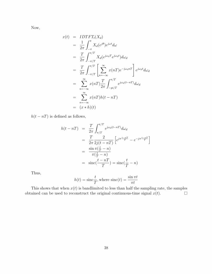
Now,

x(t) = IDTFTt(Xd)

=1

2π

∫ π

−π

Xd(ejθ)ejωtdω

=T

2π

∫ π/T

−π/T

Xd(ejωdT ejωdt)dωd

=T

2π

∫ π/T

−π/T

[∞∑

n=−∞

x(nT )e−jωdnT

]ejωdtdωd

=∞∑

n=−∞

x(nT )T

2π

∫ π/T

−pi/T

ejωd(t−nT )dωd

=∞∑

n=−∞

x(nT )h(t− nT )

= (x ∗ h)(t)

h(t− nT ) is defined as follows,

h(t− nT ) =T

2π

∫ π/T

π/T

ejωd(t−nT )dωd

=T

2π

2

2j(t− nT )

[ejπ t−nT

T − e−jπ t−nTT

]=

sin π( tT− n)

π( tT− n)

= sinc(t− nT

T) = sinc(

t

T− n)

Thus,

h(t) = sinct

T,where sinc(t) =

sin πt

πt

This shows that when x(t) is bandlimited to less than half the sampling rate, the samplesobtained can be used to reconstruct the original continuous-time signal x(t).

38

Bibliography

[1] Emmanuel Candes and Michael Wakin. An introduction to compressive sampling. IEEESignal Processing Magazine. 25(2). pp. 21 - 30. March 2008.

[2] Richard Baraniuk. Compressive sensing. IEEE Signal Processing Magazine. 24(4). pp.118-121. July 2007.

[3] Justin Romberg. Imaging via compressive sampling. IEEE Signal Processing Magazine.25(2). pp. 14 - 20. March 2008.

[4] Emmanuel Candes. Compressive sampling. Proceedings International Congress of Math-ematics. 3. pp. 1433-1452. Madrid. Spain. 2006.

[5] Emmanuel Candes and Justin Romberg. Sparsity and incoherence in compressive sam-pling. Inverse Problems. 23(3). pp. 969-985. 2007.

[6] E. J. Candes and J. Romberg. Practical signal recovery from random projections.Wavelet Applications in Signal and Image Processing XI. Proc. SPIE Conf. 5914.

[7] Emmanuel Candes and Terence Tao. Decoding by linear programming. IEEE Trans. onInformation Theory. 51(12). pp. 4203 - 4215. December 2005.

[8] David Donoho. For most large underdetermined systems of linear equations, the minimall1−norm solution is also the sparsest solution. Communications on Pure and AppliedMathematics. 59(6). pp. 797-829. June 2006.

[9] David Donoho. Compressed sensing. IEEE Trans. on Information Theory. 52(4). pp.1289 - 1306. April 2006.

[10] Emmanuel Candes, Justin Romberg, and Terence Tao, Robust uncertainty principles:Exact signal reconstruction from highly incomplete frequency information. IEEE Trans.on Information Theory. 52(2). pp. 489 - 509. February 2006.

[11] Emmanuel Candes and Terence Tao. Near optimal signal recovery from random projec-tions: Universal encoding strategies? IEEE Trans. on Information Theory. 52(12). pp.5406 - 5425. December 2006.

39

[12] Emmanuel Candes. The restricted isometry property and its implications for compressedsensing. Compte Rendus de l’Academie des Sciences. Paris. Series I. 346. pp. 589-592.2008.

[13] Venkat Chandar. A negative result concerning explicit matrices with the restricted isom-etry property. Preprint. 2008.

[14] Emmanuel Candes, Justin Romberg, and Terence Tao, Stable signal recovery from in-complete and inaccurate measurements. Communications on Pure and Applied Mathe-matics. 59(8). pp. 1207-1223. August 2006.

[15] John Wright, Allen Yang, Arvind Ganesh, Shankar Sastry and Yi Ma. Robust FaceRecognition via Sparse Representation. To appear in IEEE Transactions on PatternAnalysis and Machine Intelligence (PAMI), 2008.

[16] Allen Yang, Sameer Iyengar, Shankar Sastry, Ruzena Bajcsy, Philip Kuryloski andRoozbeh Jafari. Distributed Segmentation and Classification of Human Actions Usinga Wearable Motion Sensor Network. Workshop on Human Communicative BehaviorAnalysis. IEEE Conference on Computer Vision and Pattern Recognition (CVPR). June2008.

[17] Jeffrey Ho, Ming-Hsuan Yang, Jongwoo Lim, Kuang-Chih Lee, and David Kriegman.Clustering Appearances of Objects Under Varying Illumination Conditions. Proceed-ings of the 2003 IEEE Computer Society Conference on Computer Vision and PatternRecognition (CVPR’03)

[18] Ke Huang and Selin Aviyente. Sparse Representation for Signal Classification. Proceed-ings of Neural Information Processing Systems Conference. 2006.

[19] Dimitri Pissarenko. Eigenface-based facial recognition.

[20] M. Turk and A. Pentland. Eigenfaces for recognition. In Proceedings of IEEE Interna-tional Conference on Computer Vision and Pattern Recognition. 1991.

[21] P. Belhumeur, J. Hespanda, and D. Kriegman. Eigenfaces vs. Fisherfaces: recognitionusing class specific linear projection. IEEE Transactions on Pattern Analysis and Ma-chine Intelligence. Vol. 19. No. 7. pp. 711-720. 1997.

[22] X. He, S. Yan, Y. Hu, P. Niyogi, and H. Zhang. Face recognition using Laplacianfaces.IEEE Transactions on Pattern Analysis and Machine Intelligence. Vol. 27. No. 3. pp.328-340. 2005.

[23] Lorne Applebaum, Stephen Howard, Stephen Searle, and Robert Calderbank. ChirpSensing Codes: Deterministic Compressed Sensing Measurements for Fast Recovery.Applied and Computational Harmonic Analysis. Vol. 26. Issue 2. pp. 282-290. March2008.

40

[24] Ragib Morshed, Tzu-Yi Chen. Senior Thesis in Computer Science on compressive sens-ing based face recognition. Pomona College. 2009.

41