Theinstitutionalenvironmentfor infrastructureinvestment Seminar/ws0708/Literatur 2/22a.pdf · Theinstitutionalenvironmentfor infrastructureinvestment WitoldJ.Henisz The empirical

The institutional environment forinfrastructure investment

Witold J. Henisz

The empirical evidence that links political institutions to economic outcomes

has grown dramatically in recent years. However, virtually all of this analysis is

undertaken using data from the past three decades. This paper extends this

empirical framework by performing a two-century long historical analysis of the

determinants of infrastructure investment in a panel of over 100 countries. The

results demonstrate that political environments that limit the feasibility of policy

change are an important determinant of investment in infrastructure.

1. IntroductionThe empirical evidence that links the structure of a nation’s political institutions, andthe distribution of the preferences of the actors that inhabit them, to economicoutcomes such as an improved policy environment, investment behavior and economicgrowth has grown dramatically in recent years. However, due to data limitations,virtually all of this analysis is undertaken using data from the past three decades. Therelatively small number of years available for analysis presents serious limitations forthe interpretation of the results of these studies. Specifically, it is often difficult toseparate the effect of unobserved country characteristics, which may be correlated withor cause cross-national variation in political institutions, from the effect of theinstitutions themselves.

While some progress has been made in addressing this concern using a generalizedmethod of moment estimator (Caselli et al., 1996), this article adopts a second path. Itextends the empirical framework backward in time and performs a more thancentury-long historical analysis of the determinants of infrastructure investment in apanel of over 100 countries. The results demonstrate that political environments thatlimit the feasibility of policy change are an important determinant of cross-nationalvariation in investment in vital economic infrastructure (the number of telephonehandsets and megawatts of electrical generation)1 not only in recent years but also atthe inception of these technologies in the 19th century. The effect of cross-national andintertemporal variation in political institutions is shown to be independent of un-

Industrial and Corporate Change, Volume 11, Number 2, pp. 355–389

© ICC Association 2002

1While main telephone lines and megawatts of generating capacity would be preferable dependentvariables in the latter cases, they are unavailable for a wide sample of countries prior to the middle ofthe 20th century.

observed country-level and/or temporal variation as well as country-specific economicconditions.

Adopting an historical approach offers sufficient time series duration to separatelyidentify this effect at the cost of sacrificing the richness of data available in studies thatexamine more recent, shorter and/or less diverse samples. However, in conjunctionwith related work that finds similar effects within more limited samples of countries,regions, industries and time periods (Mansfield, 1994; Campos and Nugent, 1998;Markusen, 1998; Dawson, 1999; Rose-Ackerman and Rodden, 1999), this articleprovides additional evidence that the ability of a nation to credibly commit to a givenpolicy environment is an important component in explaining investment levels withinthat country.

These results have important ramifications for the expected diffusion rates of boththe vital components of an economy’s infrastructure, examined here, as well as thediffusion of more recent innovations, including digital communications networks.Regardless of the relevant socioeconomic, demographic or policy-related factors thatmay be thought to lead to rapid diffusion of these or other new technologies, countrieslacking a credible policy regime will be at an extreme disadvantage when competingagainst other countries for infrastructure investment. From the perspective of theinvestor, analysis of the opportunity posed by a given country for private infrastructureinvestment that neglects a sophisticated analysis of the institutional environment willconfound countries offering substantial returns on investment with those offeringsubstantial probabilities of government expropriation.

2. Theory2

2.1 Infrastructure stock and returns to capital

Although the main emphasis of this paper is on the manner in which political institu-tions affect the level of investment in telecommunications and electrical infrastructurein a given country, the analysis of political factors must also take into account the initiallevel of infrastructure stock already in place in that country. The current analysis thusshares with the macroeconomic growth literature [rooted in the models of Solow(1956) and Koopmans (1965)] the insight that a country’s existing level of capitalstock—or in this case, infrastructure penetration—determines the level of marginalreturns available from additional capital deployment and thereby influences the growthrate of the stock (see Barro, 1992).

Analogous to the arguments made in the growth literature, diminishing marginalreturns to capital are likely to be observed in panel data on infrastructure investmentsuch as employed in this study. Within a single country, over time, investment is likely totake place first in the highest return geographical areas (urban population centers) andthen slowly spread to the remainder of the country. At a moment in time across a

2Much of the discussion in this section is drawn from Henisz and Zelner (2001, 2002).

356 Witold J. Henisz

sample of countries, those countries at the frontier of infrastructure penetration mustexperiment with new technologies and invest not just in the deployment of infra-structure but also in the development of new mechanisms for infrastructure supply andnew products that may lead to additional demand. Laggard countries may, to someextent, ‘free-ride’ on the investment and experience of the countries that have precededthem.

The link between the assumption of diminishing marginal returns to capital and theproposition of an inverse relationship between infrastructure stock and infrastructuregrowth is the concept of transitional disequilibrium: countries cannot instantaneouslyattain their desired infrastructure stock-levels given changes to the political oreconomic environment. Therefore, when these environmental conditions change overtime, or vary across countries, those countries further ahead on the diffusion curve willexperience less rapid growth than ‘laggard’ countries.

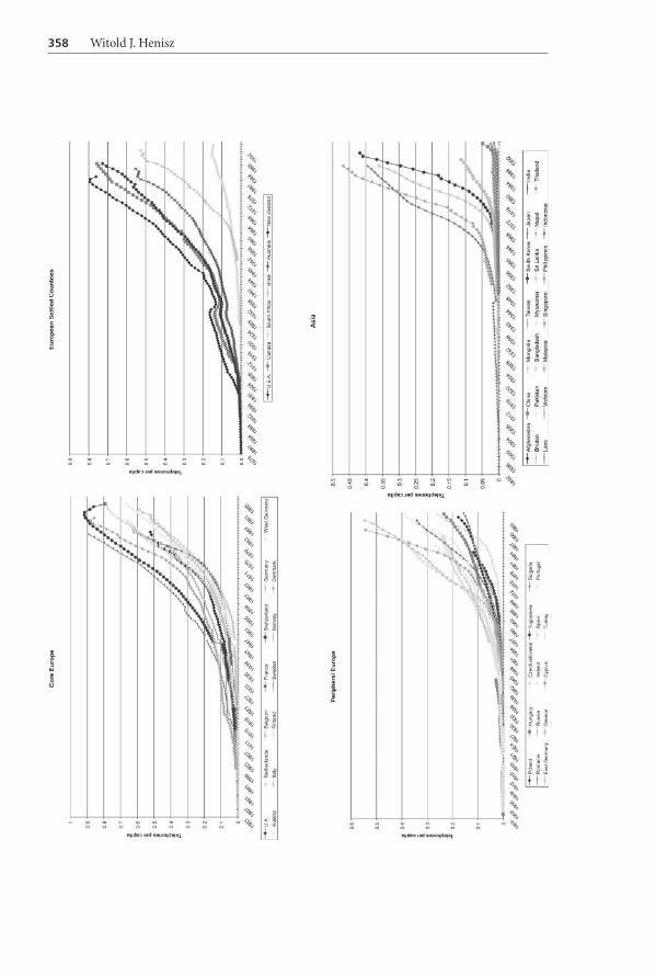
Another prominent technological driver of cross-national variation in infra-structure investment is the effect of the passage of time. Infrastructure growth-rates,like patterns of growth and diffusion of many other products and technologies (Romeo,1975; Benvignati, 1982; Gort and Klepper, 1982; Oster, 1982; Quirmbach, 1986; Levin etal., 1987; Rose and Joskow, 1990; Pennings and Harianto, 1992; Abrahamson andRosenkopf, 1993; Jovanovic and MacDonald, 1994; Thomas, 1999), likely display agedependence. Examining patterns of historical diffusion (see Figures 1 and 2) oneobserves relatively low to moderate growth rates in the initial decades after the initialpenetration of infrastructure services followed—in some countries—by a rapid accel-eration of growth and—in a handful of countries—a downward trend in penetrationbeginning in just the past few years.

While some of this pattern may correspond to variation over time in the environ-mental variables described below, the similarity to patterns of diffusion of othertechnologies points to a role for technology as well. Specifically, it may take some timeafter the availability of new infrastructure prior to widescale adoption and reorganiz-ation of economic organization to take advantage of the ubiquitous supply of theseproducers (David, 1989). Later, growth rates may stabilize or even become negative asdemand is saturated, more efficient consumption is realized and/or alternativeproducts (e.g. cellular handsets) arrive in the marketplace.

2.2 Political institutions and investment

The relationship between the stock of a country’s infrastructure and the growth rate ofthat infrastructure will be conditional on a set of country characteristics. Chief amongthese will be the country’s ability to provide a credible policy environment for investors.Theoretical support for the economic impact of political institutions has expandeddramatically in the quarter century since (North and Thomas, 1973) first outlined a‘transaction cost view of economic history.’ The crucial economic role played bysocio-political factors which reduce the costs of bargaining, contracting, monitoringand enforcement has achieved the status of conventional wisdom in economic history

The institutional environment for infrastructure investment 357


Figu

re1

Dif

fusi

onof

tele

com

mu

nic

atio

ns

infr

astr

uct

ure

.



Figu

re2

Dif

fusi

onof

elec

tric

alin

fras

tru

ctu

re.


(North and Weingast, 1989; Root, 1989; North, 1990; De Long and Shleifer, 1993;Mokyr, 1993; Landes, 1998) and development (Nelson, 1989, 1990; North, 1990; Batesand Krueger, 1993; Campos and Lien, 1994; Brunetti and Weder, 1995; Haggard andKaufman, 1995; Knack and Keefer, 1995; Sachs and Werner, 1995; World Bank, 1995;Olson, 1996; World Bank, 1996, 1997). Scholars in both these domains agree that agovernment’s ability to credibly commit to not interfere with private-property rights isinstrumental in obtaining the long-term capital investments required for countries toexperience rapid economic growth.

While these arguments are most transparent and likely strongest when consideringprivate investors, so long as public sector managers with control over investment alsoengage in subgoal pursuit, in particular the maximization of discretionary incomestreams, it is still reasonable to expect that the institutional environment will affect theincentives that managers of public sector organizations face to deploy capital. Likeprivate sector managers, public sector managers face mechanisms that limit the extentto which they can pursue their subgoals at the expense of their political and financialprincipals. However, these mechanisms are relatively weak and leave public sectormanagers with substantial latitude to pursue subgoals. Specifically, both oversight(monitoring) and incentive-based measures that are operative in the private sector areless binding on public sector managers (Cameron and Duignan, 1984; Vining andBoardman, 1989; Scott et al., 1990).

Because of the long time horizon, economies of scale and scope and highly politicalnature of the investment, infrastructure investment will be especially sensitive to acountry’s institutional environment (Williamson, 1976; Spiller, 1993; Levy and Spiller,1994; Spiller and Vogelsang, 1996; Savedoff and Spiller, 1997). Empirical work providesstrong support for this hypothesis (Grandy, 1989; Daniels and Trebilcock, 1994; Crainand Oakley, 1995; Levy and Spiller, 1996; Ramamurti, 1996; Savedoff and Spiller, 1997;Bergara Duque et al., 1998; Caballero and Hammour, 1998; Dailami and Leipziger,1998) including two examples delving into economic history by examining theconstruction of the Spanish (Keefer, 1996) and New Jersey (Grandy, 1989) railways.Two recent efforts to extend this logic to panel datasets in telecommunications (Heniszand Zelner, 2001) and electricity (Henisz and Zelner, 2002) have also found strongsupport for the hypothesis that political institutions that fail to constrain arbitrarybehavior by political actors dampen the incentive for infrastructure providers to deploycapital and, ceteris paribus, yield lower levels of per capita infrastructure investment.3

2.3 Economic characteristics.

In addition to the political forces described above, economic conditions are also likelyto play an important role in the pattern of infrastructure investment across countriesand over time. Data limitations of the century-long panel prohibit the inclusion of vari-

3In the case of electricity, the positive effect of political constraints on infrastructure investment isshown to be operative only in the presence of substantial interest group competition from industrialusers of electricity (Henisz and Zelner, 2002).


ables such as the composition of production of the economy, the cost of constructionand the demographic characteristics of the population. However, some of these factorsmay be captured by examining cross-national variation in the level of income as well asother available macroeconomic statistics.

3. Measurement and data

3.1 Political constraints

The measure of political constraints employed in this paper estimates the feasibility ofpolicy change (the extent to which a change in the preferences of any one actor may leadto a change in government policy) using the following methodology. First, extractingdata from political science databases, it identifies the number of independent branchesof government (executive, lower and upper legislative chambers)4 with veto power overpolicy change in up to 160 countries in every year from 1800 to the present. Thepreferences of each of these branches and the status quo policy are then assumed to beindependently and identically drawn from a uniform, unidimensional policy space.This assumption allows for the derivation of a quantitative measure of institutionalhazards using a simple spatial model of political interaction.

This initial measure is then modified to take into account the extent of alignmentacross branches of government using data on the party composition of the executiveand legislative branches. Such alignment increases the feasibility of policy change. Themeasure is then further modified to capture the extent of preference heterogeneitywithin each legislative branch which increases (decreases) decision costs of overturningpolicy for aligned (opposed) executive branches.

The main results of the calculations detailed in the Appendix (along with a pair ofsample calculations and values of the final index for each country in each decade) arethat (i) each additional veto point (a branch of government that is both constitutionallyeffective and controlled by a party different from other branches) provides a positivebut diminishing effect on the total level of constraints on policy change and (ii)homogeneity (heterogeneity) of party preferences within an opposition (aligned)branch of government is positively correlated with constraints on policy change. Theseresults echo those produced in similar work by Tsebelis (1995, 1999) and Butler andHammond (1996, 1997).

3.2 Other independent variables

Data on infrastructure and other non-political factors that may be thought to influenceinfrastructure investment including real per capita income, population levels and

4Previous derivations of the political constraint index described here have included an independentjudiciary and sub-federal political entities for a total of five potential veto points. Data limitationspreclude their inclusion here. The effect of their omission will be to diminish the variance amongcountries with relatively high levels of political constraints thereby dampening the magnitude of theobserved effect.


macroeconomic aggregates are taken from Mitchell (1992, 1993, 1995) and updatedusing The World Development Indicators, 1998 (World Bank, 1998).

4. Initial investmentWhat are the determinants of the timing of a country’s initial investment in infra-structure? Once the technology to transmit voice messages over copper wire had beendemonstrated by Alexander Graham Bell in 1876, or to centrally generate electric powerfor transmission by Thomas Edison in 1882, many countries quickly adopted thesetechnologies. However, outside of the United States and a core set of Europeancountries, adoption times lagged into the decades, and infrastructure growth ratesafter adoption are noticeably slower. While the level of economic development andthe relationship between a country and the core set of industrialized nations clearlyplay a role, the theoretical arguments developed above also point to an importantrelationship between political constraints and time to adoption.

4.1 Specification

In order to test this hypothesis, a discrete time logit model is employed to examine thedeterminants of the transition from having no infrastructure investment to havingsome positive quantity (Beck et al., 1998).

Let H(t) equal the probability of adoption for a country at time t. According to ourhypotheses there exist a set of country-level independent variables (w) that determineH(t).

H(t) = λw(t) (1)

So as to insure that H(t) (the probability of adoption) is bounded by 0 and 1 in theempirical results, one commonly takes a logistic transformation:

log{H(t)/[1 – H(t)]} = λw(t) (2)

Next, a separate observation record is created for every unit of time. Thus, if acountry does not have its first telephone handset until 1883, that country has a record ineach year after 1877 (the year after adoption by the United States) with a dependentvariable equal to zero (no adoption) in each year until 1883 whereafter the dependentvariable equals one (adoption). The full sample (including multiple observations forthe same entry) is then estimated using a using a maximum likelihood estimator for thetraditional logit specification. This technique addresses both the problems of censoringand time-varying explanatory variables.

Of the 6901 observed country-years with zero infrastructure penetration in telecom-munications, and the 5754 in electricity, fewer than 300 cases possess data on themacroeconomic conditions. Unfortunately, this limited sample precludes independenttesting of economic and political effects in the analysis of adoption. Economic charac-teristics will be included in the analysis of infrastructure growth presented in Section 5.The independent variables included in the vector w(t) are, however, limited to:


POLCON Political Constraint Index described in Section 3.1 and in Appen-dix 1.

COLONY A vector of colony dummies equal to one if the country was a col-ony of Great Britain, Spain, France, Belgium, Portugal or anothercolonial power in year t (not a colony is the excluded category).

REGDUM A vector of regional dummies (European settled nations, CentralAmerica & the Caribbean, South America, the Middle East, Africaand Asia with Western Europe as the excluded category).

TIMEDUM A vector of time dummies.5

4.2 Results

Table 1 displays the estimation results. With the exception of isolated colony andregional dummies, all coefficient estimates are individually significant at a P-value of0.01 or less. Additionally, an F-test confirms that the regional, colonial heritage andtemporal dummies, as individual groups, are each jointly significant at a P-value of0.01. The inclusion of the political constraint index offers a substantial improvementupon the specification in which dummy variables enter alone.6 In the case of tele-communications, the full model correctly predicts 93.8% of non-adopting years and93.4% of adopting years (93.6% overall) for an 87.1% improvement over a constantprobability assumption. Similarly, in the case of electricity, the full model correctlypredicts 89.1% of non-adopting years and 93.0% of adopting years (90.9% overall) fora 77.7% improvement over a constant probability assumption.

Table 2 displays the actual and predicted (both with and without the politicalconstraint index) year of adoption of telecommunications and electrical generationinfrastructure for each country in the sample. The improvement in the latter case ismarked. Specifically, the average error in the predicted year of initial adoption declinesfrom 8.6 years to 5.2 years in the case of telecommunications and from 8.1 to 7.0 yearsin the case of electricity.

Countries whose political structures offered relatively better protection forinternational investors than other countries in the same geographic region and with thesame colonial heritage demonstrate marked gains in the predicted time of adoption.For example, the United States had political constraint index scores of 0.39 and 0.42 inthe years in which they adopted telecommunications (1876) and electricity (1902) thatfar surpassed the average for European settled countries in these years of 0.06, 0.17 and0.21. The original prediction for adoption of telecommunications (1911) and electricity(1923) based upon geography and time alone (the United States was not a colony at thetime of adoption) were significantly improved based upon incorporation of this vital

5The hypothesis of linear or quadratic time dependence was examined but rejected in each sector.

6The F-statistics of 980 in the case of telecommunications and 380 in the case of electricity and log-likelihood ratios of 359 and 216 respectively reject the null hypothesis of the redundancy of the politicalconstraint index with a P-value of less than 0.0001.


Table 1 Estimation results for initial investment in infrastructurea

Variable Telecommunications Electricity

C –2.63

(0.01)

–4.95

(0.00)

5.14

(0.00)

3.93

(0.00)POLCON 6.07

(0.00)

3.42

(0.00)Colony of UK –1.29

(0.00)

–0.75

(0.00)

–1.76

(0.00)

–1.43

(0.00)Colony of France –2.05

(0.00)–1.68(0.00)

–1.90(0.14)

–1.70(0.00)

Colony of Belgium –2.07(0.00)

–1.69(0.00)

–0.53(0.05)

–0.30(0.26)

Colony of Portugal –0.42

(0.15)

–0.02

(0.00)

0.91

(0.00)

1.17

(0.00)Colony of other –2.55

(0.00)

–2.18

(0.00)

–1.18

(0.00)

–0.94

(0.00)European settled –0.96

(0.00)

–0.97

(0.00)

–1.41

(0.00)

–1.35

(0.00)Eastern Europe –2.91

(0.00)

–1.57

(0.00)

–3.41

(0.00)

–2.49

(0.00)Latin America –1.44

(0.00)0.09

(0.63)–3.04(0.00)

–2.25(0.00)

South America –1.01(0.00)

0.29(0.17)

–2.47(0.00)

–1.82(0.00)

Middle East –4.81

(0.00)

–3.68

(0.00)

–3.44

(0.00)

–2.55

(0.00)Asia –4.33

(0.00)

–3.18

(0.00)

–3.64

(0.00)

–2.79

(0.00)Africa –5.45

(0.00)

–4.22

(0.00)

–4.26

(0.00)

–2.55

(0.00)

N 12 633 12 633 12 552 12 552Log likelihood –2377 –2198 –2962 –2853McFadden R2 0.73 0.75 0.65 0.66% Dep = 1 50.4 50.4 59.3 59.3Correctly predicted (%) 93.0 93.6 90.9 90.9% gain 85.8 87.1 77.6 77.7

P-values are given in parentheses.aCoefficients on annual time dummies plotted in Figure 3.


Table 2 Actual and predicted years of initial investment in infrastructureboth omitting (1) and

including (2) the index of political constraints

Country Telecommunications Electricity

Actual Predicted Actual Predicted

(1) (2) (1) (2)

Afghanistan 1951 1951 1951 1951 1948 1948Algeria 1946 1960 1960 1946 1953 1953Angola 1947 1950 1950 1929 1930 1930Argentina 1913 1911 1913 1927 1929 1927Australia 1901 1911 1901 1919 1923 1920Austria 1884 1900 1884 1920 1919 1920Bangladesh 1972 1951 1951 1951 1950 1950Belgium 1896 1900 1896 1920 1919 1902Benin 1959 1959 1959 1949 1950 1950Bhutan 1972 1947 1972 1973 1941 1973Bolivia 1913 1911 1899 1937 1929 1928Botswana 1963 1951 1951 1966 1950 1950Brazil 1907 1911 1907 1928 1929 1936Bulgaria 1902 1922 1902 1924 1938 1941Burkina Faso 1959 1959 1959 1947 1950 1950Burma 1951 1948 1951 1951 1948 1951Burundi 1963 1959 1959 1965 1950 1949Cambodia 1950 1949 1949Cameroon 1950 1959 1959 1950 1950 1949Canada 1904 1911 1903 1919 1923 1923Central African Rep. 1959 1959 1959 1954 1950 1950Chad 1959 1959 1959 1953 1950 1950Chile 1900 1911 1900 1923 1929 1923China, PR 1949 1947 1948 1941 1941 1946Colombia 1913 1911 1913 1933 1929 1928Congo 1959 1959 1959 1957 1950 1950Costa Rica 1913 1913 1913 1950 1937 1930Côte d’Ivoire 1950 1959 1959 1950 1950 1950Cuba 1913 1913 1913 1928 1937 1938Cyprus 1936 1920 1926 1948 1937 1946Czechoslovakia 1920 1922 1919 1938 1941Denmark 1900 1900 1900 1920 1919 1912Dominican Rep. 1913 1913 1913 1936 1937 1928Ecuador 1903 1911 1903 1948 1929 1936Egypt 1911 1951 1951 1950 1948 1948El Salvador 1905 1913 1905 1950 1937 1938Ethiopia 1951 1949 1950 1950 1942 1942Finland 1920 1918 1917 1923 1919 1919France 1889 1900 1894 1901 1919 1902Gabon 1952 1959 1959 1952 1950 1950Germany 1888 1900 1913 1900 1919 1923Ghana 1931 1951 1951 1948 1950 1950


Table 2 Continued



(1) (2) (1) (2)

Greece 1935 1900 1922 1922 1919 1923Guatemala 1913 1913 1913 1937 1937 1938Guinea 1958 1958 1958 1950 1950 1950Guyana 1913 1920 1913 1951 1948 1948Haiti 1928 1913 1934 1950 1937 1950Honduras 1906 1913 1913 1950 1937 1929Hungary 1901 1922 1925 1923 1938 1941India 1921 1948 1948 1939 1948 1948Indonesia 1948 1947 1948 1928 1945 1946Iran 1952 1951 1952 1954 1948 1952Iraq 1949 1951 1951 1941 1948 1948Ireland 1924 1913 1920 1929 1922 1922Israel 1950 1911 1926 1949 1937 1946Italy 1883 1900 1883 1895 1919 1914Jamaica 1922 1922 1921 1937 1950 1950Japan 1892 1947 1892 1907 1941 1907Jordan 1955 1951 1955 1956 1948 1948Kenya 1925 1951 1951 1938 1950 1950Kuwait 1955 1959 1955 1955 1953 1951Laos 1955 1950 1950 1951 1950 1950Lebanon 1951 1951 1951 1943 1948 1948Liberia 1955 1949 1950 1950 1939 1946Libya 1953 1951 1951Madagascar 1947 1958 1958 1931 1950 1950Malawi 1951 1951 1951 1950 1950 1950Malaysia 1936 1951 1951 1936 1950 1950Mali 1960 1959 1959 1949 1950 1950Mauritania 1959 1959 1959 1963 1950 1950Mauritius 1951 1951 1951 1946 1950 1950Mexico 1913 1913 1913 1926 1937 1938Mongolia 1960 1947 1948 1957 1941 1946Morocco 1946 1956 1956 1946 1953 1953Mozambique 1947 1950 1950 1932 1930 1930Nepal 1961 1947 1948 1953 1941 1946Netherlands 1900 1900 1894 1919 1919 1902New Zealand 1890 1911 1890 1926 1923 1920Nicaragua 1913 1913 1913 1948 1937 1931Niger 1959 1959 1959 1950 1950 1950Nigeria 1951 1951 1951 1948 1950 1950Norway 1900 1906 1906 1920 1919 1912Oman 1965 1951 1951 1969 1948 1948Pakistan 1951 1947 1951 1951 1947 1951Panama 1913 1913 1913 1937 1937 1929Paraguay 1913 1911 1912 1941 1929 1928


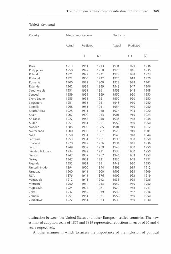
distinction between the United States and other European settled countries. The newestimated adoption years of 1876 and 1919 represented reductions in error of 35 and 4years respectively.

Another manner in which to assess the importance of the inclusion of political

Table 2 Continued



(1) (2) (1) (2)

Peru 1913 1911 1913 1931 1929 1936Philippines 1950 1947 1950 1925 1946 1935Poland 1921 1922 1921 1923 1938 1923Portugal 1922 1900 1922 1920 1919 1920Romania 1900 1922 1900 1923 1938 1941Rwanda 1962 1959 1959 1948 1947 1946Saudi Arabia 1951 1951 1951 1958 1948 1948Senegal 1959 1959 1959 1950 1950 1950Sierra Leone 1955 1951 1951 1950 1950 1950Singapore 1951 1951 1951 1948 1950 1950Somalia 1968 1951 1951 1954 1950 1950South Africa 1925 1911 1910 1924 1923 1920Spain 1902 1900 1913 1901 1919 1923Sri Lanka 1922 1948 1948 1935 1948 1948Sudan 1951 1951 1951 1950 1950 1950Sweden 1885 1900 1885 1901 1919 1912Switzerland 1900 1900 1887 1920 1919 1901Syria 1950 1951 1951 1940 1948 1944Tanzania 1953 1951 1951 1938 1950 1950Thailand 1920 1947 1936 1934 1941 1936Togo 1949 1959 1959 1948 1950 1950Trinidad & Tobago 1934 1922 1921 1933 1950 1950Tunisia 1947 1957 1957 1946 1953 1953Turkey 1947 1951 1931 1930 1948 1931Uganda 1952 1951 1951 1948 1950 1950United Kingdom 1894 1900 1894 1896 1919 1912Uruguay 1900 1911 1900 1909 1929 1909USA 1876 1911 1876 1902 1923 1919Venezuela 1912 1911 1912 1938 1929 1936Vietnam 1950 1954 1953 1950 1950 1950Yugoslavia 1924 1922 1921 1929 1938 1941Zaire 1947 1959 1959 1930 1947 1946Zambia 1951 1951 1951 1950 1950 1950Zimbabwe 1922 1951 1923 1930 1950 1930


constraints is to examine the predicted impact on the year of initial investment ininfrastructure of an improvement in (or variation in) the level of political constraintswithin a country over time (or between two otherwise identical countries at a momentin time). Ceteris paribus, ten years after the initial adoption by any country, an Africancountry that is not a colony, with political constraints, one standard deviation above themean, is more than three times as likely (0.47 vs. 0.13%) to engage in their initialinvestment in telecommunications infrastructure. The difference remains of a similarmagnitude twenty-five years after the initial adoption (4.1 vs. 1.2%) and fifty years afterthe initial adoption (38.3 vs. 14.9%). Similar effects are observed in other continentsand for infrastructure investment in electrical generating capacity. While otherunobserved country characteristics that are correlated with political constraints may bedriving these results, this initial test at least lends preliminary support to the notion thatthe credibility of a government’s policymaking apparatus plays an important role in thediffusion process of infrastructure.

5. Subsequent investmentIn order to attempt to take this alternate hypothesis into account, this section exploitspost-adoption variation in the data to examine the determinants of cross-national andintertemporal variation in infrastructure growth rates. The unbalanced panel data setscontain up to 129 countries for as many as 119 years.

Figure 3 Value of time dummies from adoption equation.


5.1 Specification

The core econometric specification employed is:

∆ INFPC i,t + COUNTRYDUMSβ 0,i + β1ln INFPCi,t–1 + β2POLCON i,t-1 +

β3(YEAR – YEAR_INIT_INFi ) + β4(YEAR – YEAR_INIT_INFi)2+

β5lnRGNPPCi,t-1+ β6COLONYi,t-1+ TIMEDUMSβ8,t + εi,t

(3)

where subscripts i and t are cross-sectional (country) and time period indices and lnsignifies the natural logarithm. Variable definitions follow from Section 4 with theaddition of:7

INFPCi,t Per capita infrastructure in country i in year t. The same modelis estimated using telephone headsets and megawatts ofelectricity generated as measures of INFPC.

YEAR Calendar year.YEAR_INIT_INFi Calendar year of initial investment in infrastructure in country

i.RGNPPCi,t Real per capita income of country i in year t expressed in 1990

US dollars.COLONYi,t Dummy variable equal to one if country i was a colony of any

country in year t.TIMEDUMS Annual time dummies.COUNTRYDUMS Country dummies.

5.2 Estimation

I have pooled across time periods and countries with the exception of (i) the countrydummies, which are necessarily pooled across time periods only and (ii) the annualtime period dummies, which are necessarily pooled across countries only.

Two econometric issues arise in estimating this equation. First, as the sample is apanel consisting of repeated observations on a broad cross-section of countries, theerror term exhibits within-group serial correlation. Second, the sample exhibits group-wise heteroskedasticity. Following Henisz and Zelner (2001, 2002), I

estimate the standard errors using a robust covariance matrix estimatorbased on that developed by Newey and West (Newey and West, 1987;Greene, 1997: 503–506). This covariance matrix estimator is consistent inthe presence of within-unit serial correlation up to a specified lag andheteroskedasticity of unknown form. Compared with the alternativeprocedure of estimating one or more AR(n) terms, the use of the robust

7Once again, potential nonlinearities in the effect of income and infrastructure stock including thepotential for nonlinearities that are dependent on the level of political constraints were explored butone can not reject the null assumption of a linear relationship in each case.


covariance matrix estimator has several advantages. First, it is compu-tationally simpler. Not only does it easily accommodate autocorrelationthat is of higher order than one, but it also simplifies estimation of modelsthat are nonlinear in the parameters. . . . Second, the robust covariancematrix estimator does not rely on an assumption that the different cross-sectional units share common autocorrelation parameters. Failure to makethis assumption in the estimation of AR(n) models creates a need toestimate many additional parameters, which reduces the efficiency of thepoint estimator. Third, it is not necessary to drop observations from one ormore time periods when using the robust covariance matrix estimator. Theestimator differs from the original Newey–West version in that it is con-structed for use in a panel setting rather than a conventional time-seriessetting (see Driscoll and Kraay (1998) and Froot (1989)). (Henisz andZelner, 2002)

A lag window of five was employed though results were robust to the use of a twoand ten year lag window.8

5.3 Results

Tables 3 and 4 report the estimation results for telecommunications and electricalgeneration capacity infrastructure respectively. The core specification described aboveis reported in column 1 of each table while columns 2–5 add other economic variablesthat might be thought to impact the demand for infrastructure. However, in each casethe coefficient estimates on these variables are statistically insignificant suggesting thatthe country fixed effects are sufficiently capturing structural differences in the sample.Columns 6–8 repeat the core specification but omit observations in the top or bottomdecile of one independent variable. As the results of primary interest are robust acrosseach of the nine specifications, I restrict my discussion to the core specification for eachcategory of infrastructure (column 1).

With the exception of the quadratic time trend in the case of telecommunications(significant at a P-value of 0.10), the dummy for colonies in the case of electricity, andthe Political Constraint Index (POLCON) in the case of electricity (significant at aP-value of 0.09) each variable is correctly signed and individually significant at aP-value of 0.02 or less. Additionally, F-tests confirm that the coefficients on the time-and country-specific fixed effects are both, as a group, jointly significant at a P-value of0.01 or less. The adjusted R2 figure is 0.108 in the case of telecommunications and 0.090in the case of electricity.

The magnitude of the economic effect of the political constraint index is moderatein size. One standard deviation in the political constraint index (0.25) leads to apredicted increase in infrastructure penetration growth of 0.8 percentage points per

8The code to perform this computation on Eviews 3.1 was generously provided by Bennet Zelner.


annum in the case of telecommunications and 0.5 percentage points per annum in thecase of electricity. While given compounding even these differences can lead todramatic differences across countries over a span of a few decades, recall that theseannual growth rate estimates exclude time-period specific, country-specific effects andthe effects of income levels and income growth rates with the latter estimated separatelyfor each country. Previous research has demonstrated that political constraints arelikely an important determinant of economic growth and, therefore, over thecentury-long period under examination here, income levels. The magnitude of thedirect economic effect computed here should therefore be considered a lower bound onthe total economic effect of political constraints on infrastructure growth.

Table 3 Estimation results for growth in telecommunications infrastructure stock

Variable (1) (2) (3) (4) (5) (6) (7) (8)

C –1.016(0.00)

–1.020(0.00)

–1.020(0.00)

–1.027(0.00)

–1.055(0.00)

–0.747(0.00)

–1.15(0.00)

–1.035(0.00)

Ln(INFPCtel,i,t) –0.068(0.00)

–0.072(0.00)

–0.072(0.00)

–0.069(0.00)

–0.071(0.00)

–0.065(0.00)

–0.073(0.00)

–0.070(0.00)

POLCON 0.033(0.01)

0.034(0.01)

0.034(0.01)

0.033(0.01)

0.033(0.01)

0.028(0.10)

0.056(0.00)

0.029(0.00)

COLONY 0.039(0.02)

0.045(0.02)

0.045(0.02)

0.040(0.02)

0.039(0.02)

0.037(0.01)

0.041(0.02)

0.040(0.03)

AT WAR? –0.031(0.03)

–0.053(0.00)

–0.052(0.00)

–0.042(0.00)

–0.041(0.00)

–0.033(0.04)

–0.037(0.03)

–0.029(0.05)

Time trend × 1000 4.529(0.00)

5.365(0.00)

5.396(0.00)

4.516(0.00)

4.655(0.00)

2.221(0.01)

4.958(0.00)

4.377(0.00)

(Time trend)2 × 1000 –0.006(0.10)

–0.008(0.06)

–0.008(0.07)

–0.006(0.16)

–0.006(0.12)

–0.001(0.74)

–0.004(0.34)

–0.003(0.49)

Ln(GDPPCt–1) 0.020(0.01)

0.012(0.18)

0.012(0.19)

0.021(0.01)

0.021(0.01)

0.021(0.01)

0.025(0.00)

0.021(0.01)

Budget deficit –0.02(0.68)

Government spending/GDP –.03(0.42)

Current account deficit/GDP –0.01(0.85)

Openness (exports +imports)/GDP

0.02(0.20)

Variable with outliersremoved

(i) (ii) (iii)

Year dummies yes yes yes yes yes yes yes yes

Fixed effects yes yes yes yes yes yes yes yes

N 4341 3753 3753 4284 4284 3913 3664 4097

Log-likelihood 2676 2470 2470 2636 2637 2621 2017 2529

Adjusted R2 0.108 0.131 0.131 0.109 0.109 0.094 0.116 0.113

P-values are given in parentheses. (i) Initial infrastructure stock; (ii) political constraints and (iii)

real per capita GDP.


6. ConclusionBy demonstrating that a sophisticated incorporation of the institutional environment

improves the power of models that predict both the initial year of infrastructure

adoption by a country and the subsequent rate of growth of that infrastructure from its

inception to the present day, this paper attempt to address the critiques that unobserved

country-level heterogeneity may be driving much of the reported correlation between

the structure of a nation’s political institutions and a broad set of economic outcomes.

Since initial adoption decisions cannot, by definition, be influenced by the existing level

of infrastructure stock, concerns regarding the role of initial conditions, combined with

Table 4 Estimation results for growth in electricity generating infrastructure

Variable (1) (2) (3) (4) (5) (6) (7) (8)

C –1.084(0.00)

–0.660(0.00)

–0.660(0.00)

–1.071(0.00)

–1.072(0.00)

–1.318(0.00)

–1.208(0.00)

–1.180(0.00)

Ln(INFPCtel,i,t) –0.100(0.00)

–0.064(0.00)

–0.064(0.00)

–0.099(0.00)

–0.099(0.00)

–0.118(0.00)

–0.107(0.00)

–0.106(0.00)

POLCON 0.022(0.09)

0.019(0.08)

0.019(0.08)

0.021(0.12)

0.021(0.13)

0.022(0.10)

0.048(0.01)

0.017(0.19)

COLONY 0.001(0.97)

0.006(0.69)

0.007(0.66)

–.007(0.71)

–.006(0.71)

–0.002(0.93)

0.005(0.75)

–0.003(0.86)

AT WAR? –0.017(0.13)

–0.022(0.06)

–0.023(0.06)

–0.017(0.18)

–0.016(0.20)

–0.015(0.18)

–0.023(0.06)

–0.020(0.09)

Time trend × 1000 6.157(0.00)

3.554(0.00)

3.514(0.00)

6.027(0.00)

6.106(0.00)

6.591(0.00)

6.775(0.00)

5.890(0.00)

(Time trend)2 × 1000 –0.017(0.02)

–0.012(0.04)

–0.012(0.04)

–0.017(0.02)

–0.018(0.02)

–0.008(0.25)

–0.024(0.01)

–0.009(0.30)

Ln(GDPPCt–1) 0.024(0.01)

0.017(0.02)

0.017(0.02)

0.025(0.00)

0.024(0.00)

0.034(0.00)

0.034(0.00)

0.031(0.00)

Budget deficit –0.054(0.27)

Government spending/GDP –0.006(0.91)

Current account deficit/GDP –0.022(0.72)

Openness (exports +imports)/GDP

0.007(0.85)

Variable with outliersremoved

(i) (ii) (iii)

Year dummies yes yes yes yes yes yes yes yes

Fixed effects yes yes yes yes yes yes yes yes

N 4816 4113 4112 4716 4716 4419 4041 4413

Log-likelihood 1182 2686 2684 1125 1124 1396 697 997

Adjusted R2 0.092 0.120 0.119 0.089 0.088 0.099 0.084 0.093

P-values are given in parentheses. (i) Initial infrastructure stock; (ii) political constraints and (iii)

real per capita GDP.


path dependency in explaining observed outcomes, are somewhat alleviated by theadoption results reported here. Similarly, the reported results showing a statistically andeconomically significant link between political institutions and infrastructure growthrates, even in a specification that includes data back to the initial adoption of theinfrastructure in a given country, as well as country- and time-specific effects, shouldalleviate concerns regarding unobserved country-level heterogeneity. Furthermore, thelack of significance of some plausible variables capturing structural differences in theseeconomies over time reinforces this conclusion.

Of course, these results are unable to account for a host of alternate economicexplanations that may play an important role. However, in conjunction with otherstudies that consider a shorter time period and are therefore able to control for theseeffects, the evidence arguing for a sophisticated treatment of political institutions in thestudy of cross-national variation in economic outcomes appears increasingly strong.

Policymakers seeking to attract investment in vital infrastructure sectors should paycareful attention to the structure of the political institutions in their country and, ifnecessary, design mechanisms to compensate for institutional shortcomings. Analog-ously, investors should analyze not just the demand for new infrastructure but also thecredibility of any and all explicit and implicit government pledges necessary to receive afair rate of return on the investment in that infrastructure.

AcknowledgementsThanks to Bennet A. Zelner for comments on a prior draft and Danielle Demianczykand David Morales for superb research assistance.

Address for correspondenceThe Wharton School, 2021 Steinberg Hall–Dietrich Hall, University of Pennsylvania,USA; [email protected].

ReferencesAbrahamson, E. and L. Rosenkopf (1993), ‘Institutional and competitive bandwagons: using

mathematical modeling as a tool to explore innovation diffusion,’ Academy of Management

Review, 18, 487–517.

Barro, R. and X. Sala-i-Martin (1992), ‘Convergence’, Journal of Political Economy, 100, 223–251.

Bates, R. H. and A. O. Krueger (eds) (1993), Political and Economic Interactions in Economic Policy

Reform: Evidence from Eight Countries. Blackwell: Cambridge, MA.

Beck, N., J. N. Katz and R. Tucker (1998), ‘Taking time seriously: time-series-cross-section

analysis with a binary dependent variable,’ American Journal of Political Science, 42, 1260–1288.

Benvignati, A. M. (1982), ‘Interfirm adoption of capital-goods innovations,’ Review of Economics

and Statistics, 64, 330–335.


Bergara D., M. E., W. J. Henisz and P. T. Spiller (1998), ‘Political institutions and electric utility

investment: a cross-nation analysis,’ California Management Review, 40, 18–35.

Brunetti, A. and B. Weder (1995), ‘Political sources of growth: a critical note on measurement,’

Public Choice, 82, 125–134.

Butler, C. K. and T. H. Hammond (1997), ‘Expected modes of policy change in comparative

institutional settings,’ Political Institutions and Public Choice Working Paper (Michigan State

University’s Institute for Public Policy and Social Research), 97.

Caballero, R. J. and M. L. Hammour (1998), ‘The macroeconomics of specificity,’ Journal of

Political Economy, 106, 724–768.

Cameron, R. L. and P. J. Duignan (1984), ‘Government owned enterprises: theory, performance

and efficiency,’ presented at New Zealand Association of Economists’ Conference, Wellington,

8 February 1984.

Campos, J. E. and D. Lien (1994), ‘Institutions and the East Asian miracle: asymmetric

information, rent-seeking and the deliberation council,’ World Bank Policy Research Paper

1321.

Campos, N. F. and J. B. Nugent (1998), ‘Investment and instability,’ mimeo.

Caselli, F., G. Esquivel and F. Lefort (1996), ‘Reopening the convergence debate: a new look at

cross-country growth empirics,’ Journal of Economic Growth, 1, 363–390.

Crain, W. M. and L. K. Oakley (1995), ‘The politics of infrastructure,’ Journal of Law and

Economics, 38, 1–17.

Dailami, M. and D. Leipziger (1998), ‘Infrastructure project finance and capital flows: a new

perspective,’ World Development, 26, 1283–1298.

Daniels, R. and M. J. Trebilcock (1994), ‘Private provision of public infrastructure: the next

privatization frontier?,’ mimeo.

David, P. A. (1989), ‘Computer and dynamo: the modern productivity paradox in the not-too-

distant mirror,’ CEPR Working Paper, Stanford University, 1–67.

Dawson, J. W. (1999), ‘Institutions, investment and growth: new cross-country and panel data

evidence,’ Economic Inquiry, 36, 603–619.

De Long, J. B. and A. Shleifer (1993), ‘Princes and merchants: European city growth before the

industrial revolution,’ Journal of Law and Economics, 36, 671–702.

Derbyshire, J. D. and I. Derbyshire (1996), Political Systems of the World. St Martin’s Press: New

York.

Driscoll, J. C. and A. C. Kraay (1998), ‘Consistent covariance matrix estimation with spatially-

dependent panel data,’ Review of Economic and Statistics, 80, 549–560.

Froot, K. A. (1989), ‘Consistent covariance matrix estimation with cross-sectional dependence

and heteroskedasticity in financial data,’ Journal of Financial and Quantitative Analysis, 24,

333–355.

Gort, M. and S. Klepper (1982), ‘Time paths in the diffusion of product innovations,’ Economic

Journal, 92, 630–653.

Grandy, C. (1989), ‘Can the government be trusted to keep its part of a social contract? New

Jersey and the railways, 1825–1888,’ Journal of Law, Economics and Organization, 5, 249–269.


Greene, W. H. (1997), Econometric Analysis. Prentice Hall: Englewood Cliffs, NJ.

Gurr, T. R. (1990), ‘Polity II: political structures and regime change, 1800–1986 [computer file],’

Boulder, CO: Center for Comparative Politics [producer], Inter-University Consortium for

Political and Social Research [distributor].

Haggard, S. and R. Kaufman (1995), The Political Economy of Democratic Transitions. Princeton

University Press: Princeton, NJ.

Hammond, T. H. and C. K. Butler (1996), ‘Some complex answers to the simple question, “do

institutions matter?”: aggregation rules, preference profiles, and policy equilibria in

presidential and parliamentary systems,’ Political Institutions and Public Choice Working

Paper (Michigan State University’s Institute for Public Policy and Social Research), 96.

Henisz, W. J. (2000), ‘The institutional environment for economic growth,’ Economics and

Politics, 12, 1–31.

Henisz, W. J. and B. A. Zelner (2001), ‘The institutional environment for telecommunications

investment,’ Journal of Economics & Management Strategy, 10, 123–148.

Henisz, W. J. and B. A. Zelner (2002), ‘Interest groups, political institutions and electricity

investment,’ mimeo.

Jovanovic, B. and G. M. MacDonald (1994), ‘Competitive diffusion,’ Journal of Political Economy,

102, 24–52.

Keefer, P. (1996), ‘Protection against a capricious state: French investment and Spanish railroads,

1845–1875,’ Journal of Economic History, 56, 170–192.

Knack, S. and P. Keefer (1995), ‘Institutions and economic performance: cross-country tests

using alternative institutional measures,’ Economic and Politics, 7, 207–227.

Koopmans, T. C. (1965), ‘On the concept of optimal growth,’ in T. C. Koopmans (ed.),

Econometric Approach to Development Planning. North Holland: Amsterdam.

Landes, D. S. (1998), The Wealth and Poverty of Nations. W. W. Norton: New York.

Levin, S. G., S. L. Levin and J. B. Meisel (1987), ‘A dynamic analysis of the adoption of a new

technology,’ Review of Economics and Statistics, 69, 12–17.

Levy, B. and P. Spiller (1996), Regulations, Institutions and Commitment. Cambridge University

Press: Cambridge.

Levy, B. and P. T. Spiller (1994), ‘The institutional foundations of regulatory commitment: a

comparative analysis of telecommunications regulation,’ Journal of Law, Economics and

Organization, 10, 201–246.

Mansfield, E. (1994), ‘Intellectual property protection, foreign direct investment and technology

transfer,’ International Finance Corporation Discussion Paper.

Markusen, J. R. (1998), ‘Contracts, intellectual property rights and multinational investments in

developing countries,’ NBER Working Paper 6448.

Mitchell, B. R. (1992), International Historical Statistics: Europe 1750–1988. Stockton Press: New

York.

Mitchell, B. R. (1993), International Historical Statistics: The Americas 1750–1988. Stockton Press:

New York.


Mitchell, B.R. (1995), International Historical Statistics: Africa, Asia & Oceania 1750–1988.

Stockton Press: New York.

Mokyr, J. (1993), British Industrial Revolution: An Economic Perspective. Westview Press: London.

Nelson, J. (1989), ‘The political economy of stabilization: commitment, capacity and public

response,’ in J. Nelson (ed.), Toward a Political Economy of Development: A Rational Choice

Perspective. University of California Press: Berkeley.

Nelson, J. (ed.) (1990), Economic Crisis and Policy Choice: The Politics of Adjustment in the Third

World. Princeton University Press: Princeton, NJ.

Newey, W. K. and K. D. West (1987), ‘A simple, positive semi-definite, heteroskedasticity and

autocorrelation consistent covariance matrix,’ Econometrica, 55, 703–708.

North, D. (1990), Institutions, Institutional Change, and Economic Performance. Cambridge

University Press: New York.

North, D. C. and R. P. Thomas (1973), The Rise of the Western World: A New Economic History.

Cambridge University Press: Cambridge.

North, D. C. and B. R. Weingast (1989), ‘Constitutions and commitment: the evolution of

institutions governing public choice in seventeenth century England,’ Journal of Economic

History, 49, 803–832.

Olson, M. (1996), ‘Big bills left on the sidewalk: why some nations are rich and others poor,’

Journal of Economic Perspectives, 10, 3–24.

Oster, S. (1982), ‘The diffusion of innovation among steel firms: the basic oxygen furnace,’ Bell

Journal of Economics, 13, 45–56.

Pennings, J. M. and F. Harianto (1992), ‘The diffusion of technological innovation in the

commercial banking industry,’ Strategic Management Journal, 13, 29–46.

Quirmbach, H. C. (1986), ‘The diffusion of new technology and the market for an innovation,’

RAND Journal of Economics, 17, 33–47.

Rae, D. W. and M. Taylor (1970), The analysis of political cleavages. Yale University Press: New

Haven, CT.

Ramamurti, R. (ed.) (1996), Privatizing Monopolies: Lessons from the Telecommunications and

Transport Sectors in Latin America. Johns Hopkins University Press: Baltimore, MD.

Rice, J. A. (1995), Mathematical Statistics and Data Analysis. Duxbury Press: Belmont, CA.

Romeo, A. A. (1975), ‘Interindustry and interfirm differences in the rate of diffusion of an

innovation,’ Review of Economics and Statistics, 57, 311–319.

Root, H. (1989), ‘Tying the king’s hands: credible commitment and royal fiscal policy during the

old regime,’ Rationality and Society, 1, 240–258.

Rose, N. L. and P. L. Joskow (1990), ‘The diffusion of new technologies: evidence from the electric

utility industry,’ RAND Journal of Economics, 21, 354–374.

Rose-Ackerman, S. and J. Rodden (1999), ‘Contracting in politically risky environments:

international business and the reform of the state,’ mimeo.

Sachs, J. and A. Werner (1995), ‘Economic convergence and economic policies,’ National Bureau

for Economic Research Working Paper 5039.

Savedoff, W. and P. Spiller (1997), ‘Commitment and governance in infrastructure sectors,’


manuscript prepared for an IDB Conference on Private Investment, Infrastructure Reform and

Governance in Latin America and the Caribbean, 15–16 September 1997.

Schwartz, E. P., P. T. Spiller and S. Urbiztondo (1994), ‘A positive theory of legislative intent,’ Law

and Contemporary Problems, 57, 51–74.

Scott, G., P. Bushnell and N. Sallee (1990), ‘Reform of the core public sector: New Zealand

experience,’ Governance, 3, 138–167.

Solow, R. (1956), ‘A contribution to the theory of economic growth,’ Quarterly Journal of

Economics, 70.

Spiller, P. (1992), ‘Agency discretion under judicial review,’ Mathematical Computer Modeling, 16,

185–200.

Spiller, P. T. (1993), ‘Institutions and regulatory commitment in utilities’ privatization,’ Industrial

and Corporate Change, 2, 387–450.

Spiller, P. T. and E. H. Tiller (1997), ‘Decision costs and strategic design of administrative process

and judicial review,’ Journal of Legal Studies, 26, 347–370.

Spiller, P. T. and I. Vogelsang (1996), ‘The institutional foundations of regulatory commitment in

the UK (with special emphasis on telecommunication),’ in P. T. Spiller, T. Pablo and I.

Vogelsang (eds), Regulations, Institutions and Commitment. Cambridge University Press:

Cambridge.

Thomas, L. (1999), ‘Adoption order of new technologies in evolving markets,’ Journal of Economic

Behavior and Organization, 38, 453–482.

Tsebelis, G. (1995), ‘Decision-making in political systems: veto players in presidentialism,

parliamentarism, multicameralism and multipartyism,’ British Journal of Political Science, 25,

289–325.

Tsebelis, G. (1999), ‘Veto players and law production in parliamentary democracies: an empirical

analysis,’ American Political Science Review, 93, 591–608.

Vining, A. R. and A. E. Boardman (1989), ‘Ownership and performance in competitive

environments: a comparison of the performance of private, mixed and state-owned

enterprises,’ Journal of Law & Economics, 32, 1–33.

Williamson, O. E. (1976), ‘Franchise bidding with respect to CATV and in general,’ Bell Journal of

Economics, 73–104.

World Bank (1995), Bureaucrats in Business: The economics and politics of government ownership.

Oxford University Press: New York.

World Bank (1996), From Plan to Market. Oxford University Press: New York.

World Bank (1997), The State in a Changing World. Oxford University Press: New York.

World Bank (1998), ‘World development indicators on CD-ROM,’ Development Data Group,

The World Bank: Washington, DC.


Appendix: deriving and constructing the political constraintsindex9

Deriving the measure of political constraints

In order to construct a structurally derived, internationally comparable measure ofpolitical constraints, the structure of political systems must be simplified in a mannerwhich allows for cross-national comparisons over a wide range of countries whileretaining the elements of that structure which have a strong bearing on the feasibility ofpolicy change. Here, I will focus on two such elements: the number of independent vetopoints over policy outcomes and the distribution of preferences of the actors thatinhabit them. Without minimizing their importance, I set aside questions of agendasetting power, decision costs (Spiller, 1992; Schwartz et al., 1994; Spiller and Tiller, 1997)and the relative political authority held by various institutions for subsequentextensions of the admittedly simplistic modeling framework presented here.

Political actors will be denoted by E (for executive), L1 (for lower house of legis-lature), L2 (for upper house of legislature).10 Each political actor has a preference,denoted by XI where I ∈ [E, L1, L2]. Assume, for the time being, that the status quopolicy (X0) and the preferences of all actors are independently and identically drawnfrom a uniformly distributed unidimensional policy space [0,1]. Data on actualpreference distributions of political actors will subsequently be incorporated into theanalysis loosening this assumption. The utility of political actor I from a policy outcomeX is assumed equal to –|X – XI| and thus ranges from a maximum of 0 (when X = XI) toa minimum of -1 (when X = 0 and XI = 1 or vice versa). Further assume that each actorhas veto power over final policy decisions. While these are, admittedly, strongassumptions, the incorporation of more refined and realistic game structures andpreference distributions presents severe complications for analytic tractability. It ishoped that, mirroring the development of the domestic positive political theoryliterature, the strength of the results obtained using the simple framework presentedhere will provide an impetus for future research.

The variable of interest to investors in this model is the extent to which a givenpolitical actor11 is constrained in his or her choice of future policies. This variable iscalculated as (1 – the level of political discretion). Discretion is operationalized as theexpected range of policies for which all political actors with veto power can agree upon

9This section draws heavily from Henisz (2000).

10Data limitations of the panel preclude the inclusion of other veto points such as an independentjudiciary, sub-federal units of power, administrative agencies, and the like.

11Without loss of generality, the remainder of the paper refers to changes in executive preferences. Notethat since the preferences of all actors and the status quo policy are drawn identically from the samedistribution, each actor, including the executive, faces the same constraints in changing policy.Allowance for the likelihood of multiple actors changing preferences simultaneously is made byincorporating information on alignment of preferences across the various branches of governmentlater in the analysis.


a change in the status quo. For example, regardless of the status quo policy, an

unchecked executive can always obtain policy XE and is guaranteed their maximum

possible utility of 0. Investors face a high degree of uncertainty since the executive’spreferences may change or the executive may be replaced by another executive with

vastly different preferences. Therefore this is categorized as a polar case in which

political discretion = 1 and political constraints equals 0 (1 – 1).

As the number of actors with independent veto power increases, the level of political

constraints increases. For example, in a country with an effective unicameral legislature

(L1), the executive must obtain the approval of a majority of the legislature in order to

implement policy changes. The executive is no longer guaranteed the policy XE as the

legislature may veto a change from the status quo policy. The executive can, at best,achieve the outcomes closest to XE that is preferred by the legislature to the status quo.

Without additional information on the preferences of the executive and the legislature

it is impossible to compute the exact outcome of the game. Nor is the expected

magnitude of the effect on political discretion of adding this additional veto point

immediately clear. However, one of the virtues of the simple spatial model outlined

above is that it provides a more objective insight into the quantitative significance ofadding an additional veto point.

Given the assumption that preferences are drawn independently and identicallyfrom a uniform distribution, the expected difference between the preferences of any

two actors can be expressed as 1/(n + 2)12 where n is the number of actors. Assuming

that there exist two political institutions with veto power [the executive (E) and a

unicameral legislature (L1)], the initial preference draw yields an expected preference

difference equal to 1/(2 + 2) = 1/4. There are six possible preference orderings in this

game (see Figure A1) that we will assume are equally likely to occur in practice.13

FigureA1 The six possible preference ordering of the game {XE, XL1}.

12See Rice (1995: 155). The intuition for this result is that the expectation of any single draw is equal to1/2 but there exists variation across draws. Given a uniform distribution, the expected distance betweenany two adjacent positions declines proportionally to the number of additional draws. The exactformula is 1/(# of draws + 1).

13For expositional convenience, I center each of the preference distributions on the unit line. As long as


In ordering (1), no change in executive preferences which retains the initial orderingof preferences yields a change in policy. The executive (XE = 1/4) prefers all policiesbetween 1/2 – ε and 0 + ε to the status quo (X0 = 1/2) while the legislature (XL1 = 3/4)prefers all policies between 1/2 + ε and 1 – ε to X0. As the executive and the legislaturecannot agree on a change in policy, political discretion (the feasibility of policy change)equals 0 and political constraints equal 1. The same argument is true by symmetry forordering (2). In the remaining orderings, both the executive and legislature agree on adirection in which policy should move relative to the status quo X0. These cases haveclosed form solutions other than the status quo policy. Their exact values depend on theassumption as to who moves first (or last) and the relative costs of review by each party.

However, in the absence of knowledge on the rules of the game in each country, therange of outcomes over which both parties can agree to change the status quo is used asa measure of political discretion. As this range expands, there exists a larger set of policychanges preferred by both political actors with veto power. The existence of such a setreduces the credibility of any given policy and therefore decreases the level of politicalconstraints. In ordering (3), the executive (XE = 1/2) prefers policies between 1/4 + εand 3/4 – ε to the status quo (X0 = 1/4) while the legislature (XL1 = 3/4) prefers allpolicies greater than 1/4 + ε. There exists a range of policies approximately equal to 1/2(between 1/4 + ε and 3/4 – ε), which both actors agree are superior to the status quo.The political discretion measure for this ordering therefore equals 1/2 yielding apolitical constraints measure equal to 1/2. The same is true in orderings (4), (5) and (6).The expected level of political constraints for the game {XE, XL1} based on the numberof veto points alone is the average of the political constraint measures across the sixpossible preference orderings: (1 + 1 + 1/2 + 1/2 + 1/2 + 1/2)/6 = 2/3.

Note that this initial measure of political constraints is based solely on the number ofde jure veto points in a given polity maintaining the strong and unrealistic assumptionof uniformly distributed preferences. However, neither the constitutional existence ofveto power nor its prior exercise provide a de facto veto threat in the current period.Specifically, loosening the assumption of uniformly distributed preferences by allowingfor preference alignment (i.e. majority control of the executive and the legislature by thesame party) would be expected to expand the range of political discretion and therebydecrease the level of political constraints. In order to allow for this effect, the purelyinstitutional measure of political constraints described above is supplemented withinformation on the preferences of various actors and their possible alignments. Forexample, if the legislature were completely aligned with the executive, the game wouldrevert back to our simple unitary actor discussed above with a constraint measure of 0.The same exercise of determining constraints given the assumption of either com-

the expected difference between any two preferred points remains 1/4, the quantitative results areinsensitive to the absolute location of these points. For example, were the leftmost (rightmost) point ineach distribution to be placed at 0 (1) rather than 1/4 (3/4), the quantitative results would beunchanged.


pletely independent or completely aligned actors was conducted for all observed in-

stitutional structures yielding the values for political constraints displayed in Table A1.

Further modifications are required when other political actors are neither

completely aligned with nor completely independent from the executive. In these cases,

the party composition of the other branches of government are also relevant to the level

of constraints. For example, if the party controlling the executive enjoys a majority in

the legislature, the level of constraints is negatively correlated with the concentration of

that majority. Aligned legislatures with large majorities are less costly to manage and

control than aligned legislatures that are highly polarized.

By contrast, when the executive is faced with an opposition legislature, the level of

constraints is positively correlated with the concentration of the legislative majority. A

heavily fractionalized opposition may provide the executive with more discretion due

to the difficulty in forming a cohesive legislative opposition bloc to any given policy.

Information on the partisan alignment of different government branches and on the

difficulty of forming a majority coalition within them can therefore provide valuable

information as to the extent of political constraints.

Suppose, for example, that the party controlling the executive completely controls

the other branch(es) of government (100%14 of legislative seats). In this case, the values

displayed in the appropriate right-hand column of Table A1 are utilized. However, as

the executive’s need for coalition building and maintenance increases (his or her

majority diminishes), and under the assumption that the same party controls both

branches, the values converge to the levels displayed in the left-most column. For the

case in which the branches are controlled by different parties, the results are reversed.

Now, complete concentration by the opposition (100% legislative seats) leads to the

assignment of the values in the left-most column. As the opposition’s difficulty of

forming coalitions increases, the values converge to the levels displayed in the

appropriate right-hand column. Following an extensive body of literature in political

Table A1 Political constraints with complete independence/alignment

Independent political

actors

Entities completely aligned with executive

None (L1 or L2) L1 and L2

E 0E, L1 2/3 0E, L1, L2 4/5 2/3 0

E, executive; L1, lower legislature; L2, upper legislature.

14I assume that as the majority diminishes from this absolute level the difficulty in satisfying the prefer-ences of all coalition or faction members increases thus increasing the level of political constraints.


science on the costs of forming and maintaining coalitions, the rate of convergence isbased upon the extent of legislative fractionalization (Rae and Taylor, 1970).

The fractionalization of the legislature is equal to the probability that two randomdraws from the legislature are from different parties. The exact formula is:

(4)

where n = the number of parties, ni = seats held by nth party and N = total seats.The final value of political constraints for cases in which the executive is aligned with

the legislature(s) is thus equal to the value derived under complete alignment plus thefractionalization index multiplied by the difference between the independent andcompletely aligned values calculated above. For cases in which the executive’s party is inthe minority in the legislature(s), the modified constraint measure equals the valuederived under complete alignment plus (one minus the fractionalization index)multiplied by the difference between the completely independent and dependent valuescalculated above. In cases of mixed alignment, a weighted (equally) sum of the relevantadjustments is used.

For example, in the case described above the constraint measure equaled 0 if thelegislature was completely aligned and 2/3 if it was completely independent. However, ifthe same party controls the executive and the legislative chamber and the probability oftwo random draws from the legislature belonging to different parties equals 1/4 (theexecutive has a large majority in parliament) then the modified constraint measureequals 0 + 1/4 × (2/3 – 0) = 1/6. By contrast, if the executive relied on a heavily fraction-alized coalition in which the probability that any two random draws were from differentparties was 75%, the modified constraint measure would equal 0 + 3/4 × (2/3 – 0) = 1/2.In the case where the opposition controls the legislature the values would be reversed. Aheavily concentrated majority by the opposition would lead to a value of 0 + (1 – 1/4) ×(2/3 – 0) = 1/2 while a fractionalized legislature would receive a score of 0 + (1 – 3/4) ×(2/3) = 1/6.

This measure of political constraints has one important virtue that also yields severalweaknesses. The strength of the measure is that it is structurally derived from a simplespatial model of political interaction which incorporates data on the number ofindependent political institutions with veto power in a given polity and data on thealignment and heterogeneity of the political actors that inhabit those institutions. Thefirst weakness of the measure is that its validity is based upon the validity of theassumptions imposed upon the spatial model in order to generate quantitative results.Another weakness is that many features of interest are left out of the model includingagenda setting rights, decision costs, other relevant procedural issues, the political roleof the military and/or church, cultural/racial tensions, and other informal institutionswhich impact economic outcomes.

11

11

−−

−

L

N

MMM

O

Q

PPP=

∑ni

niN

Ni

n b g


Constructing the measure of political constraints

Construction of a measure of political constraints based on the above methodologyrequires three types of data. First, information regarding the number of institutionalplayers in a given polity; second, data on partisan alignments (including coalitions)across institutions; and, finally, data on the party composition of legislatures. Allcountries were assumed to have an executive. Data on the existence of other politicalactors (unicameral or bicameral legislatures15) with substantive veto power was takenfrom the Polity database and Derbyshire and Derbyshire (1996).

The above data sources were then supplemented by various issues of The PoliticalHandbook of the World and The Statesman’s Yearbook to note the party distribution of thelegislature(s): specifically, whether the executive enjoys a majority in one (or both)legislature(s) and how many seats in each legislature were controlled by each party. Basedon this information, the values of institutional constraints were modified to form ameasure of political constraints using the methodology described in the previous section.

Sample calculation

Like the hypothetical example above, in 1990 Guyana had two veto points (anindependent executive and a single legislative chamber). However, the same party (thePeople’s National Congress) controlled the presidency and held 42 of the 53 legislativeseats, with the remaining seats distributed among three other parties. The probabilitythat two random draws from the legislature would be from different parties (thefractionalization index) was 35.4%. As a result, the initial constraint measure of 2/3 wasscaled downwards to 0.237 to take into account the (imperfect) alignment of thelegislative chamber with the executive branch. [Specifically, the final measure of 0.237 is35.4% of the distance between the measure with no veto points or perfect alignment(0.000) and the value of the measure with one veto point and perfect opposition (2/3).]

In 1993, Guyana held an election in which the People’s Progress Party won thePresidency and the majority in the legislature. The new distribution of seats was 35 forthe People’s Progress and 27 for the People’s National Party, with the remaining parties’seat totals unchanged. In this case, the probability that two random draws from thelegislature would belong to different parties increased to 54.5%, making it relativelymore difficult for the new governing party to steamroll the legislature in comparison totheir immediate predecessor (i.e. their majority was slightly more tenuous). Thepolitical constraint measure thus rose from 0.237 to 0.365 (or 54.5% of the distancebetween the value with no veto points or perfect alignment and the value with one vetopoint and perfect opposition). Table A2 reports the decade average of the result of theanalogous calculation for each country where the necessary data exist. Figure A2 plotsthe regional averages by year.

15Effective legislatures possess ‘significant governmental autonomy . . . including, typically, substantialauthority with regard to taxation and disbursement, and the power to override vetoes of legislation.’ Aclassification of partially effective is assigned when ‘the effective executive’s power substantiallyoutweighs but does not completely dominate that of the legislature.’ (Gurr, 1990: 51)


Table A2 Decade averages for political constraint indexa

Country 1880–89

1890–99

1900–09

1910–19

1920–29

1930–39

1940–49

1950–59

1960–69

1970–79

1980–89

1990–98

Afghanistan 0.00 0.00 0.00 0.00 0.00 0.00 0.00 0.00 0.00 0.00 0.00 0.00Albania 0.00 0.00 0.00 0.00 0.00 0.00 0.00 0.00 0.22Algeria 0.00 0.00 0.00 0.00 0.00 0.00 0.00 0.00 0.00 0.00 0.00 0.00Angola 0.00 0.00 0.00 0.00 0.00 0.00 0.00 0.00 0.00 0.00 0.08Argentina 0.47 0.44 0.57 0.08 0.00 0.00 0.22 0.57Armenia 0.29Australia 0.00 0.00 0.41 0.34 0.45 0.46 0.43 0.44 0.52 0.47 0.48 0.47Austria 0.06 0.06 0.13 0.43 0.13 0.15 0.46 0.42 0.42 0.43 0.43Azerbaijan 0.00Bahrain 0.00 0.00 0.00Bangladesh 0.00 0.00 0.00 0.00 0.00 0.00 0.00 0.00 0.01 0.00 0.38Belarus 0.00Belgium 0.38 0.37 0.47 0.48 0.52 0.48 0.54 0.49 0.48 0.55 0.69 0.70Benin 0.00 0.00 0.00 0.00 0.00 0.00 0.00 0.00 0.00 0.00 0.00 0.06Bhutan 0.00 0.00 0.00 0.00 0.00 0.00 0.00Bolivia 0.29 0.39 0.71 0.00 0.16 0.07 0.05 0.00 0.29 0.40Bosnia 0.00Botswana 0.00 0.00 0.00 0.00 0.00 0.00 0.00 0.00 0.12 0.23 0.15 0.27Brazil 0.00 0.00 0.06 0.00 0.00 0.55 0.18 0.00 0.35 0.13Bulgaria 0.00 0.20 0.08 0.00 0.00 0.00 0.00 0.00 0.36Burkina Faso 0.00 0.00 0.00 0.00 0.00 0.00 0.00 0.00 0.00 0.00 0.00 0.00Burma 0.00 0.00 0.00 0.00 0.00 0.00 0.00 0.00 0.05 0.00 0.00 0.00Burundi 0.00 0.00 0.00 0.00 0.00 0.00 0.00 0.00 0.11 0.00 0.00 0.00Cambodia 0.00 0.00 0.00 0.00 0.00 0.00 0.00 0.00 0.00 0.00 0.00 0.09Cameroon 0.00 0.00 0.00 0.00 0.00 0.00 0.00 0.00 0.00 0.00 0.00 0.27Canada 0.30 0.33 0.32 0.32 0.39 0.41 0.43 0.38 0.42 0.39 0.40 0.45Central African Rep. 0.00 0.00 0.00 0.00 0.00 0.00 0.00 0.00 0.00 0.00 0.00 0.30Chad 0.00 0.00 0.00 0.00 0.00 0.00 0.00 0.00 0.00 0.00 0.00 0.00Chile 0.00 0.23 0.69 0.31 0.10 0.00 0.57China 0.00 0.00 0.00 0.00 0.00 0.00 0.00 0.00 0.00 0.00 0.00 0.00Colombia 0.00 0.00 0.00 0.37 0.45 0.40 0.19 0.41 0.37 0.41 0.45Comoros 0.00 0.00 0.00Congo 0.00 0.00 0.00 0.00 0.00 0.00 0.00 0.00 0.00 0.00 0.00 0.28Costa Rica 0.00 0.00 0.25 0.31 0.35 0.35 0.32 0.40 0.38 0.38Cuba 0.00 0.00 0.00 0.00 0.00 0.00 0.00 0.00 0.00 0.00 0.00 0.00Cyprus 0.00 0.00 0.00 0.00 0.00 0.00 0.00 0.00 0.00 0.10 0.20 0.35Czech Republic 0.58Czechoslovakia 0.00 0.00 0.00 0.00 0.27 0.65 0.00 0.00 0.00 0.00 0.00 0.34Denmark 0.42 0.27 0.39 0.43 0.51 0.45 0.29 0.53 0.49 0.53 0.54 0.53Dominican Rep. 0.00 0.00 0.00 0.00 0.17 0.00 0.00 0.00 0.09 0.26 0.42 0.58Ecuador 0.00 0.00 0.00 0.00 0.00 0.00 0.00 0.27 0.14Egypt 0.00 0.00 0.00 0.00 0.00 0.00 0.00 0.00 0.00 0.00 0.00 0.00El Salvador 0.00 0.00 0.00 0.00 0.00 0.09 0.27 0.24 0.45Equatorial Guinea 0.00 0.00 0.00 0.00Eritrea 0.00Estonia 0.55Ethiopia 0.00 0.00 0.00 0.00 0.00 0.00 0.00 0.00 0.00 0.00 0.00 0.00Finland 0.00 0.00 0.00 0.14 0.52 0.50 0.50 0.53 0.54 0.55 0.54 0.54France 0.26 0.42 0.51 0.55 0.50 0.45 0.49 0.53 0.70 0.55 0.49 0.44Gabon 0.00 0.00 0.00 0.00 0.00 0.00 0.00 0.00 0.00 0.00 0.00 0.00Gambia, The 0.26 0.19 0.21 0.09Georgia 0.17East Germany 0.00 0.00 0.00 0.00 0.00Germany 0.11 0.10 0.09 0.15 0.56 0.13 0.43West Germany 0.47 0.44 0.39 0.39 0.40Ghana 0.00 0.00 0.00 0.00 0.00 0.00 0.00 0.00 0.00 0.05 0.04 0.00Greece 0.21 0.22 0.00 0.38 0.26 0.16 0.36 0.38Guatemala 0.00 0.00 0.00 0.00 0.07 0.07 0.00 0.00 0.16 0.32


TableA2 Continued

Country 1880–89

1890–99

1900–09

1910–19

1920–29

1930–39

1940–49

1950–59

1960–69

1970–79

1980–89

1990–98

Guinea 0.00 0.00 0.00 0.00 0.00 0.00 0.00 0.00 0.00 0.00 0.00 0.12Guinea-Bissau 0.00 0.00 0.17Guyana 0.00 0.00 0.00 0.00 0.00 0.00 0.00 0.00 0.40 0.33 0.00 0.27Haiti 0.00 0.00 0.00 0.00 0.09 0.00 0.00 0.00 0.12Honduras 0.00 0.00 0.00 0.00 0.28 0.10 0.00 0.04 0.23 0.07 0.21 0.34Hungary 0.00 0.00 0.00 0.00 0.00 0.00 0.08 0.00 0.00 0.00 0.00 0.41Iceland 0.52 0.47 0.46 0.43 0.48 0.49 0.51 0.51India 0.00 0.00 0.00 0.00 0.00 0.00 0.00 0.34 0.39 0.42 0.52Indonesia 0.00 0.00 0.00 0.00 0.00 0.00 0.00 0.02 0.00 0.00 0.00 0.00Iran 0.00 0.00 0.00 0.00 0.00 0.00 0.00 0.00 0.00 0.00 0.00 0.00Iraq 0.00 0.00 0.00 0.00 0.00 0.00 0.00 0.00 0.00 0.00 0.00 0.00Ireland 0.00 0.00 0.00 0.00 0.39 0.44 0.42 0.45 0.42 0.40 0.41 0.46Israel 0.00 0.00 0.00 0.00 0.00 0.00 0.05 0.55 0.54 0.48 0.49 0.53Italy 0.50 0.45 0.33 0.07 0.00 0.10 0.57 0.48 0.47 0.49 0.50Ivory Coast 0.00 0.00 0.00 0.00 0.00 0.00 0.00 0.00 0.00 0.00 0.00 0.09Jamaica 0.00 0.00 0.00 0.00 0.00 0.00 0.00 0.03 0.39 0.37 0.24 0.26Japan 0.00 0.71 0.71 0.00 0.42 0.46 0.52 0.52 0.56Jordan 0.00 0.00 0.00 0.00 0.00 0.00 0.00 0.00 0.00 0.00 0.00 0.00Kazakhstan 0.00Kenya 0.00 0.00 0.00 0.00 0.00 0.00 0.00 0.00 0.00 0.00 0.00 0.29Kuwait 0.00 0.00 0.00 0.00 0.00 0.00 0.00 0.00 0.00 0.00 0.00 0.00Kyrgyz Republic 0.05Laos 0.00 0.00 0.00 0.00 0.00 0.00 0.00 0.00 0.00 0.00 0.00Latvia 0.35Lebanon 0.00 0.00 0.00 0.00 0.00 0.00 0.00 0.00 0.12 0.12 0.04 0.08Lesotho 0.24 0.00 0.00 0.00Liberia 0.00 0.00 0.00 0.00 0.00 0.00Libya 0.00 0.00 0.00 0.00 0.00 0.00 0.00 0.00 0.00 0.00 0.00 0.00Lithuania 0.34Luxembourg 0.22 0.20 0.31 0.22 0.46 0.50 0.47 0.36Macedonia 0.27Madagascar 0.00 0.00 0.00 0.00 0.00 0.00 0.00 0.00 0.11 0.01 0.00 0.26Malawi 0.00 0.00 0.00 0.00 0.00 0.00 0.00 0.00 0.00 0.00 0.00 0.19Malaysia 0.00 0.00 0.00 0.00 0.00 0.00 0.00 0.00 0.38 0.38 0.48 0.31Mali 0.00 0.00 0.00 0.00 0.00 0.00 0.00 0.00 0.00 0.00 0.00 0.26Mauritania 0.00 0.00 0.00 0.00 0.00 0.00 0.00 0.00 0.00 0.00 0.00 0.00Mauritius 0.00 0.00 0.00 0.00 0.00 0.00 0.00 0.00 0.44 0.43 0.37 0.30Mexico 0.00 0.00 0.00 0.00 0.00 0.00 0.00 0.02 0.07 0.12 0.19 0.37Moldova 0.09Mongolia 0.00 0.00 0.00 0.00 0.00 0.00 0.00 0.00 0.00 0.00 0.00 0.10Morocco 0.00 0.00 0.00 0.00 0.00 0.00 0.00 0.00 0.00 0.00 0.00 0.15Mozambique 0.00 0.00 0.00 0.00 0.00 0.00 0.00 0.00 0.00 0.00 0.16Namibia 0.37Nepal 0.00 0.00 0.00 0.00 0.00 0.00 0.00 0.00 0.00 0.00 0.00 0.37Netherlands 0.41 0.42 0.52 0.55 0.58 0.66 0.60 0.42 0.62 0.52 0.49 0.51New Zealand 0.35 0.32 0.38 0.41 0.38 0.34 0.34 0.33 0.32 0.34 0.35Nicaragua 0.00 0.00 0.00 0.00 0.12 0.00 0.00 0.00 0.00 0.00 0.37Niger 0.00 0.00 0.00 0.00 0.00 0.00 0.00 0.00 0.00 0.00 0.00 0.13Nigeria 0.00 0.00 0.00 0.00 0.00 0.00 0.00 0.00 0.25 0.00 0.05 0.00North Korea 0.00 0.00 0.00 0.00 0.00 0.00 0.00 0.00 0.00 0.00 0.00 0.00North Yemen 0.00 0.00 0.00 0.00 0.00 0.00 0.00 0.00 0.00 0.00 0.00 0.00Norway 0.32 0.38 0.37 0.45 0.52 0.48 0.46 0.44 0.46 0.48 0.45 0.51Oman 0.00 0.00 0.00 0.00 0.00 0.00 0.00 0.00 0.00 0.00 0.00 0.00Pakistan 0.00 0.00 0.00 0.00 0.00 0.00 0.00 0.00 0.13 0.00 0.07 0.46


Table A2 Continued

Country 1880–89

1890–99

1900–09

1910–19

1920–29

1930–39

1940–49

1950–59

1960–69

1970–79

1980–89

1990–98

Panama 0.00 0.00 0.00 0.27 0.34 0.21 0.20 0.22 0.00 0.00 0.23Papua New Guinea 0.34 0.50 0.36Paraguay 0.00 0.00 0.00 0.00 0.30 0.04 0.00 0.00 0.00 0.00 0.00 0.19Peru 0.00 0.00 0.00 0.00 0.00 0.12 0.17 0.00 0.15 0.06Philippines 0.00 0.00 0.00 0.00 0.00 0.04 0.00 0.33 0.46 0.07 0.09 0.62Poland 0.00 0.00 0.00 0.01 0.29 0.00 0.00 0.00 0.00 0.00 0.00 0.39Portugal 0.00 0.00 0.00 0.00 0.00 0.00 0.00 0.21 0.43 0.39Qatar 0.00 0.00 0.00Romania 0.27 0.00 0.00 0.00 0.00 0.00 0.00 0.46Russia 0.00 0.00 0.00 0.00 0.00 0.00 0.00 0.00 0.00 0.00 0.00 0.06Rwanda 0.00 0.00 0.00 0.00 0.00 0.00 0.00 0.00 0.00 0.00 0.00 0.00Saudi Arabia 0.00 0.00 0.00 0.00 0.00 0.00 0.00 0.00 0.00 0.00 0.00 0.00Senegal 0.00 0.00 0.00 0.00 0.00 0.00 0.00 0.00 0.00 0.00 0.00 0.00Serbia 0.00 0.00 0.00 0.00 0.00 0.00 0.00 0.00 0.46Sierra Leone 0.00 0.00 0.00 0.00 0.00 0.00 0.00 0.00 0.31 0.14 0.06 0.00Singapore 0.00 0.00 0.00 0.00 0.00 0.00 0.00 0.00 0.23 0.00 0.02 0.05Slovakia 0.50Slovenia 0.56Somalia 0.00 0.00 0.00 0.00 0.00 0.00 0.00 0.00 0.11 0.00 0.00 0.00South Africa 0.00 0.00 0.00 0.42 0.42 0.32 0.47 0.41 0.28 0.32 0.20 0.35South Korea 0.00 0.00 0.00 0.00 0.00 0.00 0.00 0.00 0.03 0.00 0.04 0.22South Vietnam 0.00 0.00 0.00 0.00 0.00 0.00 0.00 0.00 0.00 0.00South Yemen 0.00 0.00 0.00 0.00 0.00 0.00 0.00 0.00 0.00 0.00 0.00Spain 0.00 0.00 0.00 0.00 0.00 0.26 0.00 0.00 0.00 0.12 0.46 0.49Sri Lanka 0.00 0.00 0.00 0.00 0.00 0.00 0.00 0.50 0.38 0.20 0.40Sudan 0.00 0.00 0.00 0.00 0.00 0.00 0.00 0.00 0.19 0.00 0.00 0.00Swaziland 0.00 0.00 0.00 0.00Sweden 0.32 0.39 0.38 0.45 0.51 0.56 0.52 0.53 0.45 0.47 0.47 0.49Switzerland 0.30 0.29 0.35 0.35 0.28 0.55 0.70 0.70 0.70 0.70 0.70 0.46Syria 0.00 0.00 0.00 0.00 0.00 0.00 0.00 0.00 0.00 0.00 0.00 0.00Taiwan 0.00 0.00 0.00 0.00 0.00 0.00 0.00 0.00 0.11 0.19 0.34Tajikistan 0.00Tanzania 0.00 0.00 0.00 0.00 0.00 0.00 0.00 0.00 0.00 0.00 0.00 0.08Thailand 0.00 0.00 0.00 0.00 0.00 0.00 0.00 0.00 0.00 0.05 0.63 0.29Togo 0.00 0.00 0.00 0.00 0.00 0.00 0.00 0.00 0.00 0.00 0.00 0.18Trinidad & Tobago 0.00 0.00 0.00 0.00 0.00 0.00 0.00 0.00 0.26 0.34 0.40 0.40Tunisia 0.00 0.00 0.00 0.00 0.00 0.00 0.00 0.00 0.00 0.00 0.00 0.00Turkey 0.00 0.00 0.00 0.00 0.00 0.57 0.55 0.20 0.35 0.23 0.23 0.37Turkmenistan 0.00Uganda 0.00 0.00 0.00 0.00 0.00 0.00 0.00 0.00 0.21 0.00 0.00 0.07Ukraine 0.11United Arab Emirates 0.00 0.00 0.00United Kingdom 0.40 0.44 0.42 0.46 0.36 0.33 0.37 0.37 0.34 0.36 0.35 0.36Uruguay 0.73 0.52 0.44 0.57 0.44 0.10 0.21 0.54USA 0.40 0.43 0.39 0.40 0.39 0.35 0.46 0.40 0.38 0.40 0.60 0.47Uzbekistan 0.00Venezuela 0.00 0.00 0.00 0.00 0.00 0.00 0.00 0.00 0.54 0.34 0.39 0.31Vietnam 0.00 0.00 0.00 0.00 0.00 0.00 0.00 0.00 0.00 0.00 0.00 0.00Yemen 0.00Yugoslavia 0.00 0.00 0.00 0.00 0.10 0.00 0.00 0.00 0.00 0.00 0.00 0.00Zaire 0.00 0.00 0.00 0.00 0.00 0.00 0.00 0.00 0.00 0.00 0.00 0.00Zambia 0.00 0.00 0.00 0.00 0.00 0.00 0.00 0.00 0.00 0.00 0.00 0.00Zimbabwe 0.00 0.00 0.00 0.00 0.00 0.00 0.00 0.08 0.00

aAnnual data for each country are available at http://www-management.wharton.upenn.edu/

henisz/.


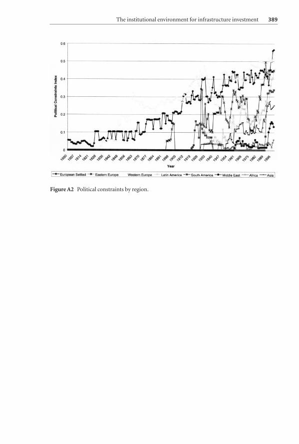
FigureA2 Political constraints by region.


Documents

Theinstitutionalenvironmentfor infrastructureinvestment Seminar/ws0708/Literatur 2/22a.pdf · Theinstitutionalenvironmentfor infrastructureinvestment WitoldJ.Henisz The empirical