Embed Size (px)
Citation preview

the use of single sensors in
seismic acquisition processing
and interpretation
The use of single sensors in seismic acquisition
processing and interpretation
Proefschrift
ter verkrijging van de graad van doctor
aan de Technische Universiteit Delft
op gezag van de Rector Magnificus Prof dr ir JT Fokkema
voorzitter van het College voor Promoties
in het openbaar te verdedigen
op vrijdag 19 oktober 2007 om 1500 uur
door
Ionelia PANEA
Magister in Geology
University of Bucharest geboren te Caracal-Olt Romania
Dit proefschrift is goedgekeurd door de promotor
Prof dr ir J T Fokkema
Toegevoegd promotor Dr ir GG Drijkoningen
Samenstelling promotiecommissie
Rector Magnificus voorzitter Prof drir JTFokkema Technische Universiteit Delft promotor Dr ir G G Drijkoningen Technische Universiteit Delft toegevoegd promotor Prof drir CP Wapenaar Technische Universiteit Delft Prof drir S Cloetingh Vrije Universiteit Amsterdam Prof drir A-J van der Veen Technische Universiteit Delft Prof drir C Dinu Boekarest Universiteit Dr R Stephenson Vrije Universiteit Amsterdam Dr Randell Stephenson heeft als begeleider in belangrijke mate aan de totstandkoming van dit proefschrift bijgedragen Copyright copy 2007 by I Panea Delft University of Technology Delft The Netherlands All rights reserved No part of this publication may be reproduced stored in a retrieval system or transmitted in any form or by any means electronic mechanical photocopying recording or otherwise without the prior written permission of the author Support
Printed b
The research reported in this thesis has been financially supported by the Netherlands Research Center of Integrated
y Curtea Veche in Romania
to my family
Contents
Contents i Summary v Samenvatting vii List of symbols xi 1 Introduction 1 11 Background 1 12 Literature review 4 13 Thesis aim and outline 7 2 Problem statement for single-sensor data in acquisition processing and interpretation 9 21 Introduction 9 22 Seismic acquisition 11 221 Standard array-forming 13 2211 One array response without and with variations 15 2212 Multiple arrays without and with variations 19 222 Multiple arrays for a field situation 24 23 The use of single sensors in data processing 29 24 The use of single sensors in geological interpretation 35
ii
25 Conclusions 40 3 The use of single sensors in data acquisition Minimum Variance Distortionless Response (MVDR) beamformer 43
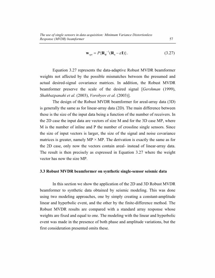
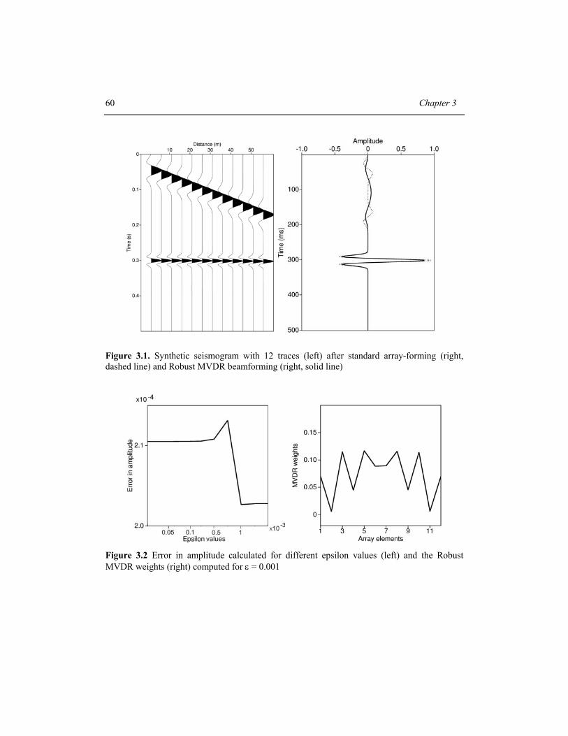
31 Introduction 43 32 Design of a Robust MVDR beamformer 46 33 Robust MVDR beamformer on synthetic single-sensor seismic data 57 331 Robust MVDR on 2D modeled single-sensor seismic data without variations 58 332 Robust MVDR on 2D modeled single-sensor seismic data with variations 67 333 Robust MVDR on 2D finite-difference modeled single-sensor seismic data 76 334 Robust MVDR on 3D finite-difference modeled single-sensor seismic data 84 34 Robust MVDR beamformer on single-sensor field data 88 341 Robust MVDR on 2D single-sensor field data 89 342 Robust MVDR on partial-3D single-sensor field data 93
343 Data processing of the 3D standard array-forming and 3D Robust MVDR beamforming responses 96
35 Conclusions 100
4 The use of single sensors in processing stereotomography 103 41 Introduction 103 42 Background to the post-stack stereotomography 106
43 Application of post-stack stereotomography on a single-sensor seismic dataset recorded in a low signal-to-noise area 115
iii
431 Seismic dataset Acquisition and pre-processing 115 432 Imaging using standard CMP-based approach 121
433 Imaging using post-stack stereotomography 122 434 2D versus 2D from cross-line stacked partial-3D data 131 44 Conclusions 138
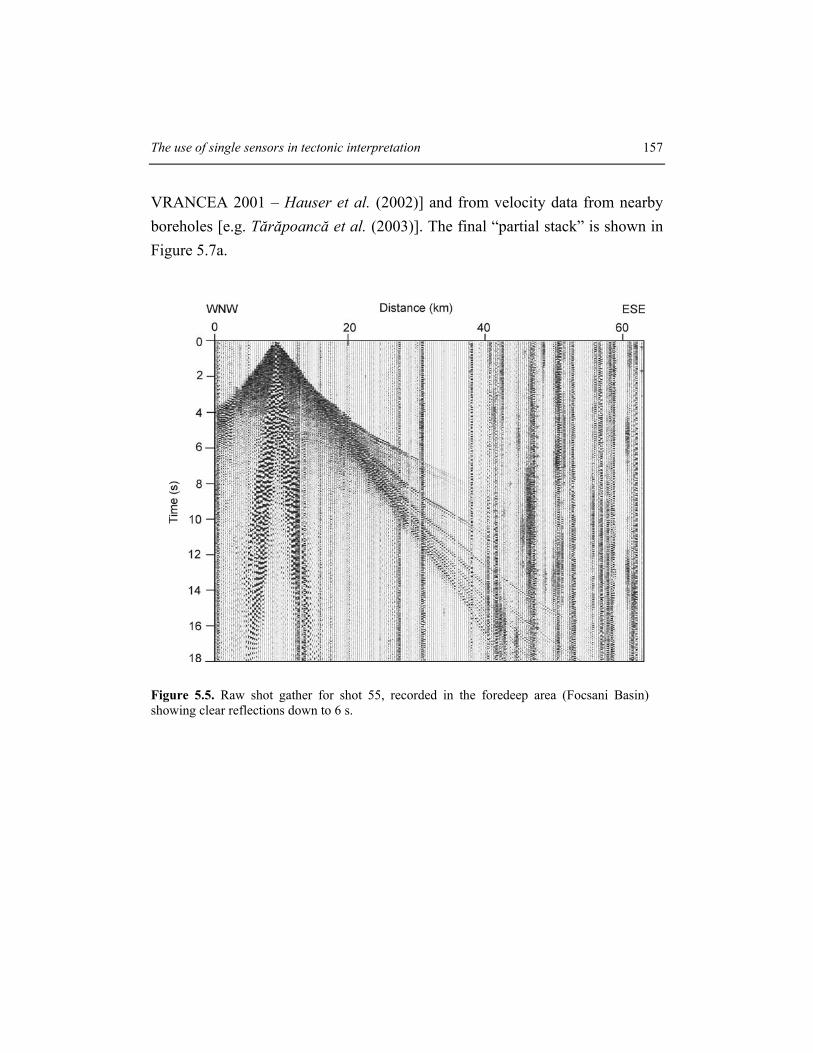
5 The use of single sensors in tectonic interpretation 141 51 Introduction 141 52 Geological setting 149 53 Seismic data ndash field acquisition processing and results 152 531 Processing for the upper crust reflectivity (ldquopartial-stackrdquo) 154 532 Interpretation of the ldquopartial-stackrdquo 159 533 Processing for lower crust reflectivity (ldquofull-stackrdquo) 162 534 Interpretation of the ldquofull-stackrdquo 176 54 Conclusions 182 6 Conclusions 185 Appendix A1 193 A11 The one-dimensional Fourier Transform in time and space 193 A12 The two-dimensional Fourier Transform 195 Appendix A2 197 Appendix A3 199 Bibliography 203
ii
Acknowledgements 215 About the author 217
Summary
The quality of the results of a seismic reflection project is strongly dependent on the data acquisition parameters Once the data are recorded we cannot undo some of the artifacts of the acquisition such as spatial aliasing and hard-wired array forming However in the digital domain we can undo some of the acquisition artifacts in processing by adding extra processing steps andor using different parameters and algorithms So in general it is desirable to move the digital world to the sensing element as much as possible
The use of single sensors in data acquisition processing and (tectonic) interpretation is studied in this thesis In data acquisition the quality difference between single sensors and hard-wired arrays depends on the characteristics of the studied area (eg surface topography) Via modeling we show the effect of the topography on the reflection responses of single sensors and (hard-wired) standard arrays We also analyze the effect of amplitude and phase variations on the array responses knowing that these types of variations can occur in field situations Using fine spatially sampled single-sensor recordings we obtain an improved array response after some corrections have been applied In this way we demonstrate the efficacy of the use of single sensors for data acquisition instead of hard-wired arrays
Analyzing the noise attenuation performed by standard arrays we propose a more efficient algorithm used to enhance the signal-to-noise ratio of array response called the Minimum Variance Distortionless Response (MVDR)
vi
beamformer This is a type of beamformer that adapts itself to the data and therefore allows flexibility in its use The beamformer creates weights of the different elements of the array while for a standard array the weights are just 1 The beamformer is steered by the global characteristics of a record and uses this information to do local spatially adaptive beamforming We show that in all cases studied on synthetic as well as field data the MVDR beamformer is superior to the standard array in the sense that the MVDR showed better noise attenuation The algorithm has been used for 2D and 3D datasets where the highest gain is achieved in 3D
Two field single-sensor datasets are studied in this thesis First one was a part of a shallow seismic reflection project and the second one a part of a deep seismic reflection and refraction project Their recording was done using fine spatially sampled single sensors in the first case and coarse single sensors in the second case Since the presence of the surface waves is important on the shallow seismic dataset the MVDR algorithm was used to enhance the signal-to-noise ratio of array responses Next the accuracy of the 2D velocity model used for stacking and migration of the data was increased using the post-stack stereotomography
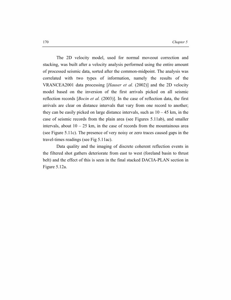
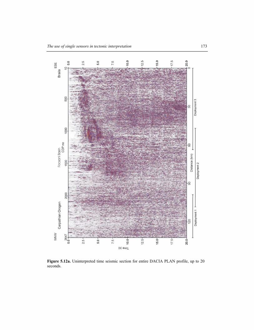
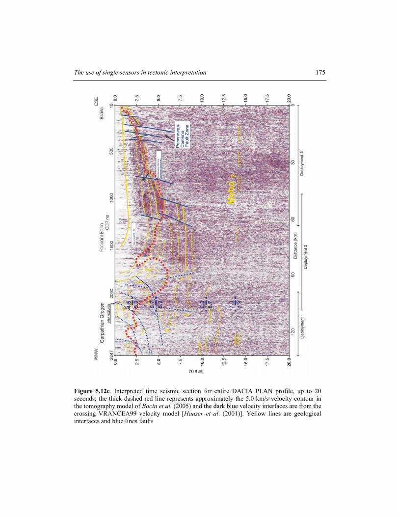
The single-sensor deep seismic reflection dataset was recorded with the purpose to study the crustal structure in the bending zone of Carpathians Data processing is done following two directions namely the processing for the upper and lower crust reflectivity Both time sections were used for tectonic interpretation that provided new interesting structural features in the subsurface in the curvature zone of Carpathians which has not been detected before and seems consistent with other deep-refraction studies
Samenvatting
De kwaliteit van de resultaten van een seismisch reflectie-experiment hangt sterk af van de data-acquisitie parameters Als de data eenmaal zijn vastgelegd is het niet meer mogelijk om bepaalde artefacten van de acquisitie zoals een onvoldoende fijne ruimtelijke bemonstering en fysieke groepvorming ongedaan te maken Echter in het digitale domein is het wel mogelijk om sommige artefacten van de acquisitie ongedaan te maken door het toevoegen van extra bewerkingsstappen enof het gebruiken van andere parameters en algoritmen In het algemeen is het dus wenselijk om de digitalisering zo ver als mogelijk door te zetten naar de opname apparatuur in het veld
Het gebruik van enkele sensoren in data-acquisitie bewerking en (tektonische) interpretatie is het onderwerp van studie in dit proefschrift Bij data-acquisitie hangt het kwaliteitsverschil tussen opnames gemaakt met enkele sensoren en fysieke groepen van sensoren af van de karakteristieken van het onderzochte gebied (bijv de topografie aan de oppervlakte) Middels modeleren laten we het effect zien dat de topografie heeft op de reflectierespons van enkele sensoren en standaard (fysieke) groepen Tevens analyseren we het effect van variaties in amplitude en fase op de groeprespons dit soort variaties treedt in het veld namelijk vaak op Wanneer we gebruik maken van opnamen gedaan met enkele sensoren in een fijne ruimtelijke bemonstering verkrijgen we na het toepassen van enige correcties een verbeterde groeprespons Op deze
viii
wijze tonen we de doeltreffendheid aan van het gebruik van enkele sensoren ten opzichte van fysieke groepen van sensoren
Aan de hand van het bestuderen van de ruisverzwakking verkregen met standaard groepen stellen we een efficieumlnter algoritme voor om de signaalruis verhouding van de groeprespons te verbeteren genaamd de Minimum Variantie Vervormingloze Respons (MVDR) beamformer Dit type beamformer past zichzelf aan de data aan en is derhalve flexibel in gebruik De beamformer creeumlert gewichten voor ieder element van een groep terwijl bij een standaard groep de gewichten gewoon eacuteeacuten zijn De beamformer wordt gestuurd door de globale karakteristieken van een opname en gebruikt deze informatie om lokaal een ruimtelijk afhankelijke beamforming toe te passen We tonen aan dat in alle bestudeerde gevallen op zowel synthetische data als data opgenomen in het veld de MVDR beamformer beter werkt dan de standaard groep op het gebied van ruisverzwakking Het algoritme is gebruikt op 2D en 3D datasets de grootste verbetering treedt op in 3D
Twee enkele-sensor datasets uit het veld zijn in dit proefschrift bestudeerd De eerste is afkomstig uit een onderzoek naar ondiepe seismische reflecties en de tweede uit een onderzoek naar diepe seismische reflecties en refracties In het eerste geval werden de opnamen gemaakt met behulp van enkele sensoren met een fijne ruimtelijke bemonstering in het andere geval was de ruimtelijke bemonstering grof Aangezien oppervlaktegolven dominant aanwezig zijn op de data voor ondiepe seismiek werd het MVDR algoritme gebruikt om de signaalruis verhouding van de groepresponsies te verbeteren Vervolgens werd de nauwkeurigheid van het 2D lsquostackingrsquo en migratie snelheidsmodel vergroot middels lsquopost-stackrsquo stereotomografie
De dataset met diepe reflecties werd opgenomen met enkele ontvangers met als doel het bestuderen van de structuur in de aardkorst bij de plooiingszone van de Karpaten De data werden twee keer verwerkt om een
ix
optimaal beeld te verkrijgen van de contrasten in het bovenste en onderste gedeelte van de aardkorst De twee tijdsecties die dit opleverde werden beide gebruikt voor tektonische interpretatie waarbij nieuwe structuren in de ondergrond van de plooiingszone van de Karpaten werden opgemerkt die consistent lijken met bevindingen uit andere onderzoeken voor diepe refracties
viii
List of symbols
a ndash steering vector α ndash emergence angle in stereotomography βS ndash takeoff angle to the source S βR ndash takeoff angle to the receiver R d ndash vector of single-element observations do ndash vector of analytic complex signal di
r ndash real stereotomographic dataset di
c ndash computed stereotomographic dataset etx ndash error in the (t x)-domain efk ndash error in the (f kx)-domain ε ndash positive constant f ndash frequency h ndash half offset kn ndash horizontal wavenumber of the noise kN ndash Nyquist wavenumber kM ndash rejection notch wavenumber kx ndash wavenumber in the spatial direction x λs ndash horizontal wavelength of the signal λn ndash horizontal wavelength of the noise λ1 ndash Lagrange multiplier λ2 ndash Lagrange multiplier
xii
m ndash model part in stereotomography n ndash noise vector psx ndash slope on the common-shot gather prx ndash slope on the common-receiver gather ρ - density s ndash desired signal vector so ndash analytic complex signal t ndash time to ndash zero-offset travel-time tSR ndash two-way travel-time tCRS ndash CRS-stacking operator τ ndash delay in time v ndash velocity vo ndash near-surface velocity w ndash weight vector wopt ndash optimal weight vector x ndash space xo ndash output position in stereotomography xCMP ndash midpoint position y ndash MVDR beamformer response yo ndash desired array response ys ndash standard-array or MVDR beamformer response ỹo ndash (f kx)-domain amplitude spectrum of the desired array response ỹs ndash (f kx)-domain amplitude spectrum of the standard-array or MVDR beamformer response z - depth A ndash transfer function of receiver array Anorm ndash normalized transfer function of receiver array
xiii
C ndash velocity field Ds ndash matrix that contain the desired signal Dn ndash matrix that contain noise ∆ ndash error matrix ∆t ndash travel-time interval ∆x ndash single-sensor spacing ∆xp ndash distance interval E ndash output power En ndash noise power Es ndash signal power I ndash identity matrix J ndash number of B-spline functions L ndash array length L1(w λ1) ndash Lagrangian function L2(w λ2) ndash Lagrangian function M ndash number of array elements in in-line direction N ndash normal wave in stereotomography NIP ndash Normal-incidence-point wave in stereotomography Nt ndash number of time samples Ne ndash number of picked travel-times Nf ndash number of frequency samples Nk ndash number of wavenumber samples Nk_old ndash number of wavenumber samples computed for single-sensor spacing Nk_new ndash number of wavenumber samples computed for desired group interval P ndash number of array elements in cross-line direction Po ndash acquisition point RN ndash radius of the N wavefront RNIP ndash radius of the NIP wavefront
xii
Rps ndash presumed signal covariance matrix Rs ndash signal covariance matrix Rn ndash noise covariance matrix Rd ndash data covariance matrix R ndash sample covariance matrix R ndash receiver position S ndash source position SNR ndash signal-to-noise ratio
T ndash transpose
TS ndash two-way travel-time to source S TR ndash two-way travel-time to receiver R Va ndash apparent horizontal velocity Vp ndash P-wave velocity Vs ndash S-wave velocity X ndash reflecting diffracting point
Chapter 1
Introduction 11 Background
The seismic reflection method is the most successful method to explore and monitor hydrocarbon reservoirs from the surface It has been used for decades in this industry starting in the beginning of the 1900rsquos In the early days one single sensor was a big investment and no exploration industry existed Only during that century seismic was used more and more to explore the subsurface and many big oil and gas fields were discovered using single-sensor recordings In the 1960rsquos two advances came the common-midpoint (CMP) method and the advent of the computer (Mayne 1962) Also during that time the sensors had become much smaller and allowed arrays to be used Arrays had the task to reduce noise on land being mainly surface waves they act as discrete spatial filters in the field Regarding the aliased frequencies the recording station contains an anti-alias filter that removes the frequencies greater than the Nyquist frequency In addition the arrays were supposed to reduce the amount of data since a multi-channel system of 16 channels in the 1960rsquos was seen as
2 Chapter 1
high-tech Since those days arrays existed while the number of channels increased and increased over time Nowadays systems of 10000 channels are not uncommon A further advance in understanding the tasks of arrays was put forward in the 1980rsquos It was recognized that the seismic receivers were supposed to sample the wavefield properly [Ongkiehong and Askin (1988)] At that time it was recognized that the number of channels was not sufficient to have proper sampling so arrays were identified as spatial anti-alias filters and resampling operators Nowadays with 10000-channel systems this spatial sampling can be fully done in 3D and array operations can be done digitally rather than in an analog way (the old-fashioned hard-wired array)
In the more academically oriented field of crustal seismology the developments were not supported by a rich industry but have been stimulated by more fundamental geological questions During the last century many active seismic surveys have taken place to unravel the structure of the earth as a whole After the international ban on nuclear tests the sources were less extreme but large sources such as large air guns and large amounts of dynamite are still being used for exploring the crust of the earth Also in this field arrays were introduced to reduce the source-induced noise ie surface waves Many of the DEKORP lines going through Germany were recorded with arrays In Romania arrays are also used to monitor the regional seismic activity [Ghica et al (2005)] But also here the number of channels increased and so allowed a fuller recording of the whole wavefield although mostly being 2D recordings In this field arrays are not always used the reason being that if the topography or shallow subsurface is heavily structured the array may work as a damper rather than a reflector-enhancer This is typically happening in hilly or mountainous areas where elevation statics are significant It is known that reflections (wave propagating vertically into the earth) are more sensitive to statics compared to surface waves (wave propagating horizontally)
The use of single sensors in seismic acquisition processing and interpretation 3
In this thesis we will model analyze and process single-sensor recordings for these two settings for exploration (Chapters 2 3 and 4) and for crustal seismology (Chapter 5) In the last decades various modeling codes were designed in order to get synthetic seismograms for complex subsurface geometries and for arbitrary source-receiver separations The complexity of the modeling codes varies from the convolution between an input wavelet and a reflection time series to for example the fourth-order-finite difference modeling of the P- and S-waves The results of the synthetic dataset pre-processing modeled with single sensors or array of sensors for a studied area can influence the choice of the data acquisition parameters (Chapter 2) Single-sensor spacing is considered an important parameter since it is a source of spatial aliasing in case of slow seismic arrivals (eg surface waves) Data without spatial aliasing are data sampled to more than two points per wavelength otherwise the wave arrival direction becomes ambiguous Aliasing can occur on the axes of time depth geophone shot midpoint offset or crossline but in practice is the worst on the horizontal space axes The efficiency of some of the processing algorithms is influenced by spatial aliasing such as f-k filtering and migration (spatial deconvolution) There are algorithms that work good in the presence of aliased data belonging to the class of beamformers they are applied to increase the signal-to-noise ratio of seismic records (Chapter 3)
In time the algorithms designed for migration increased in complexity Migration could only be done digitally in the 1970rsquos which has now developed in full pre-stack depth-migration in 3D Also here the data reduction as achieved by arrays in the field helps in the migration process In our era single-sensor recordings is still too expensive to do in a pre-stack depth-migration since the amount of data would become eg twelve-fold determined by the number of receivers in one array It is expected that in the future this will
4 Chapter 1
become a feasible option A gain here would be is that higher-resolution images can be obtained using single-sensor recordings The possibility will be shown in Chapter 5 12 Literature review
Single sensors are often used in the data acquisition especially in deep seismic surveys Nowadays the fine spatially sampled single sensors tend to replace the arrays of receivers used in the acquisition of shallow data It is known that arrays of sensors and sources are considered very efficient in coherent noise attenuation [Newman and Mahoney (1973) Morse and Hildebrandt (1989) Cooper (2004)] An array sums the signals from a pattern of sources or receivers to attenuate various noises while attempting to preserve as much of the reflection signal as possible [Stone (1994)] The design of an array is done taking into account that the single-sensor spacing must allow a proper recording of the noise (eg surface waves) and the group interval spacing must allow a proper recording of the reflected waves [Vermeer (1990)] a proper recording meaning arrivals with no spatial aliasing Also it is known that shorter array emphasizes signal preservation while the longer array places priority on noise rejection [Hoffe et al (2002)] Modeling results showed that the hard-wired array response can be synthesized using fine spatially sampled single sensors recordings The phase and amplitude variations occur due to the field conditions (rough topography significant lateral velocity variations irregular sensors spacing imperfection in ground-coupling) These variations affect the real dataset [Hoover and OrsquoBrien (1980) Krohn (1984) Drijkoningen (2000) Muyzert and Vermeer (2004) Drijkoningen et al (2006) Capman et al (2006)] The use of single-sensor recordings to synthesize the standard array response allows a data pre-processing (eg static corrections)
The use of single sensors in seismic acquisition processing and interpretation 5
that can attenuate the effect of such variations [Hoffe et al (2002) Capman et al (2006)] In this way the signal-to-noise ratio of array response is enhanced also the reflected waves are protected This is considered one advantage of the use of single-sensors in data acquisition with important effect on the data processing and interpretation results
The arrays of sensors are used in many fields such as sonar radar microphone array speech processing [Capon et al (1967) Cox (1973) Gershman et al (1995) Gershman et al (2000)] seismology [Ozbek (2000)] wireless communications [Godara (1997) Rapapport (1998)] Their elementary recordings are input data to different algorithms (eg beamforming) proposed to attenuate various noise contributions Different types of beamformers were designed depending on the type of noise that has to be attenuated The simplest one is known as delay-and-sum beamformer [Johnson et al (1993)] The complexity of the beamformers increased in order to be able to adapt to any type of mismatches between the designing approaches and real data [Cox (1973) Godara (1986) Cox et al (1987) Feldman and Griffiths (1994) Wax and Anu (1996) Bell et al (2000) Shahbazpanahi et al (2003)] In the exploration seismology Ozbek (2000) proposed a type of beamformer that can be used to attenuate various types of coherent noise encountered in seismic data acquisition and processing This type of beamformer can be thought as an adaptive f-k filter that is fixed in those parts of the (f k)-amplitude spectrum that contain the signal to be protected and adaptive in the rest of it
Sometimes the signal-to-noise ratio of the seismic recordings can be low even if single sensors or arrays are used in data acquisition The lack of clear reflections on the pre-stack data can decrease the accuracy of the standard velocity analysis Based on this many algorithms were proposed in order to obtain a reliable velocity model used for stacking and migration
6 Chapter 1
Stereotomography is an example of such algorithm It belongs to the class of the slope methods and it can be applied on pre-stack [Billette and Lambareacute (1998) Chauris et al (2002) Chalard et al (2002) Billette et al (2003) Lambareacute et al (2003) Lambareacute et al (2004)] and post-stack domains [Lavaud et al (2004)] Both algorithms have been applied on synthetic and marine dataset The application of the pre-stack stereotomography is restricted to the datasets recorded using the same spacing between single sensors and sources The advantage of the post-stack stereotomography is that its application does not require the same spacing between single sensors and sources and the automatic traveltime picking is done on a Common-Reflection-Surface (CRS) stack that is characterized by a higher signal-to-noise ratio due to stacking of traces from super common-midpoint gathers The computation of the CRS stack also allows the computation of a control triplet parameter (α RNIP RN) where α is the emergence angle of the zero-offset ray RNIP and RN are the radii of the wavefront curvatures [Muumlller (1999) Mann et al (1999) Jaeger et al (2001) Trappe et al (2001)] They all are associated with two hypothetical waves namely the so-called normal wave (N) and the normal-incident-point wave (NIP) The CRS stack is a model independent seismic imaging method that can be performed without any ray tracing and macro-velocity model estimation The knowledge of the near surface velocity is required [Jaeger et al (2001)] It has been demonstrated that the CRS stack produces high-resolution time-domain sections and post-stack depth migration of CRS stacks may be considered as an alternative to pre-stack depth migration in areas of high difficulties (eg complicate tectonic structure) [Hubral (1999) Trappe et al (2001)]
The use of single sensors in seismic acquisition processing and interpretation 7
13 Thesis aim and outline
The aim of this thesis is to study the effectiveness of the use of single sensors and arrays of sensors in areas with different topographies Also starting from the modeling results regarding to the surface waves attenuation performed by standard arrays we present an algorithm that will perform a better attenuation of the un-desired energy contained by single-sensor records Throughout the thesis the standard array response is equivalent with the hard-wired array response Using fine spatially sampled single-sensor records as input data this response can be synthesized in two steps First we sum a number of traces equal with the desired number of array elements and then the output is spatially resampled to the desired group interval
The results of the analysis of synthetic and field single-sensor records will be presented in this thesis In Chapter 2 we compare the processing and tectonic interpretation results of two modeled datasets The first one is represented by single-sensor recordings and the second one is represented by recordings with standard array responses Both datasets are modeled in the presence of phase variations introduced by significant elevation statics and irregular spacing of single sensors The elevation profile used in modeling is based on the field situation described in Chapter 5 The standard array responses are computed following the procedure described above
In the next chapter we will describe a new algorithm the Minimum Variance Distortionless Response (MVDR) beamformer which can be applied on 2D and 3D single-sensor records in order to attenuate the undesired energy We define as undesired energy all energy present at wavenumbers greater than the Nyquist wavenumber computed for the desired group interval We start with the analysis of single-sensor records modeled for simple depth models and then we increase the model complexity in order to get various types of waves
8 Chapter 1
Since the field records are affected by the amplitude and phase variations due to the field conditions we model single-sensor records in the presence of these variations then we apply the MVDR beamforming in order to see how efficient is its noise attenuation in such conditions At the end of Chapter 3 the standard array-forming and MVDR beamforming are applied on a single-sensor shallow dataset Since the field data quality is low a new tomographic method is used to determine the velocity model required by stacking and depth migration This is the subject of Chapter 4 The results of two different approaches are presented here namely the Common-Midpoint approach and the Common-Reflection-Surface-stereomography approach
The effectiveness of the use of single sensors in tectonic interpretation will be shown in Chapter 5 We use a single-sensor deep dataset recorded along a profile that started and crossed the mountainous and hilly areas and ended in the plain area Different processing directions are followed in order to get the best structural image possible
Finally conclusions are drawn in Chapter 6
Chapter 2
Problem statement for single-sensor data in acquisition processing and interpretation
21 Introduction The quality of land seismic data depends on many factors In first instance it is important to set the acquisition parameters such as the distances right But even if these parameters are correctly set how the geophones are deployed can influence the signal-to-noise ratio of the seismic recordings Land seismic data contain many un-desired arrivals that can be cumbersome to attenuate during the data processing The most important type of noise is the so-called ground roll being surface or Rayleigh waves they occur because of the presence of the (stress-free) surface and near-surface layers Surface waves are characterized by low apparent velocities and small frequencies compared to the reflected waves These arrivals are sometimes recorded using improper acquisition parameters since only proper recording of the reflected waves is performed An example of such a parameter is the geophone spacing that in general is chosen too large for the proper recording of the surface waves As a result these slow arrivals are affected by spatial aliasing which creates
10 Chapter 2
problems during the data processing (eg filtering migration) and interpretation Other non-standard acquisition is a variation in field conditions creating phase and amplitude variations across an array A common way used for decades to attenuate the surface waves is the use of hard-wired receiver arrays [Newman and Mahoney (1973) Hoffe et al (2002) Cooper et al (2004)] Two parameters are crucial in the array design namely the spacing between array elements and the size of group interval The first one is chosen so that a proper sampling of the surface waves is allowed and the second one it is chosen so that a proper sampling of the reflected waves is allowed In both cases it is desired to have recordings without any spatial aliasing In the last two decades the use of hard-wired arrays is more and more questioned and acquisition using finely spatially sampled single sensors is more being used [Burger et al (1998) Baeten et al (2000)] Then the conventional array response can be easily synthesized in two steps Using this type of input dataset the array response is synthesized in two steps First we sum a number of single-sensor recordings equal to the desired number of array elements Then we resample the result to the desired group interval the size of the desired group interval has to be chosen so that the desired signal will not be spatial aliased In this chapter we show that in case of significant field variations within arrays using arrays in the standard way is not good enough for example attenuation of the surface waves There are situations when the remaining noise seen on the first step of array-forming will be heavily spatially aliased after resampling Looking at the array response in the time domain we will see some remaining wavelets sometimes of significant amplitude and frequency they can be seen as ldquoedge-effectsrdquo of the array and should be attenuated because they degrade the quality of array response In addition the standard arrays do
Problem statement for single-sensor data acquisition processing and interpretation 11
not work properly in the presence of variations being caused by local variations in the field (coupling statics) 22 Seismic acquisition In this section we will show that the use of conventional hard-wired arrays in hilly and mountainous areas will have a negative effect on the reflections Their response can be analyzed by modeling different field situations In addition we will analyze the effect of phase and amplitude variation on the array response Both types of variation affect the real dataset due to the field conditions [Hoover and OrsquoBrien (1980) Krohn (1984) Drijkoningen (2000) Hoffe et al (2002) Panea et al (2003) Panea et al (2004) Panea and Drijkoningen (2006) Capman et al(2006)] Phase variations are mainly caused by traveltime variations These are introduced by rapid near-surface variations and could via processing be corrected with static corrections if the data allow (if arrays are used it will not be possible to process them this way) In statics the effect of the near subsurface is assumed to be a pure time delay and these delays are surface consistent implying that each trace at a given location gets the same time delay [Cox (1999)] The near surface affects the seismic data in several ways For example the lateral velocity variations in the near surface and variations in layer thickness or topography can cause variations in the arrival times and amplitudes of the upcoming events [Capman et al (2006)] The presence of the sub-surface and near-surface layers allows for the generation of the most important type of noise recorded on land data namely the ground-roll It was said that the use of suitable array patterns can suppress partially ground-roll [Morse and Hildebrandt (1989)] Recent studies have shown that the array response can be less or even strongly distorted by increasing of the complexity
12 Chapter 2
of the overburden rapid lateral velocities variations on the scale of an array [Muyzert and Vermeer (2004)] Amplitude variations are caused mainly by imperfect ground-coupling of geophones The problem of coupling has been extensively studied in the last decades using modeling tests and field experiments [Lamar (1970) Hoover and OrsquoBrien (1980) Krohn (1984) Tan (1987) Drijkoningen (2000) Drijkoningen et al (2006)] The term coupling defines a phenomenon that affects energy transfer The coupling of a geophone to the ground involves the quality of the plant how firmly these two are in contact and also considerations of the geophonersquos weight and base area because the geophone-ground coupling system as natural resonances and introduces a filtering action [Sheriff (1991)] According to theory the geophone-ground coupling is the difference between the velocity measured by the geophone and the velocity of the ground without the geophone This so-called definition of the ground-coupling was used for theoretical models it is also used for the design of geophones so that optimal characteristics can be found [Drijkoningen (2000)] The practicing geophysicist takes into account the imperfections of the coupling of the geophones with its surroundings As a consequence the definition written above becomes Bad geophone coupling is the difference between the velocity as measured by the badly planted geophone and the velocity as measured by the well-planted geophone [Drijkoningen (2000)] Measurements of the geophone-ground coupling for vertical and horizontal geophones have been done in the laboratory and in the field [Krohn (1984) Drijkoningen (2000)] Their results showed that the geophone accurately follows the ground motion for lower frequencies than the coupling resonant frequency In case of higher frequencies the coupling can alter both the amplitude and phase of the seismic signal The coupling resonant frequency for vertical geophones is determined by the firmness of the soil [Krohn (1984)] Based on the experiment results it was accepted that for
Problem statement for single-sensor data acquisition processing and interpretation 13
conventional seismic recordings the use frequencies less than 100 Hz and vibrational amplitudes less than 10-2 cms the normal planting of vertical geophones in firm soil is acceptable For higher frequency recordings or for surveys that take place in areas with loose soil the geophone should be buried in order to achieve better coupling In addition the laboratory experiments showed that the length of the geophone spike affects the coupling [Krohn (1984)] The effect of ground-coupling was studied in both domains time and frequency using different field datasets [Drijkoningen (2000)] 221 Standard array-forming It is well-known that an array sums the signals coming from a pattern of receivers or sources to attenuate various types of noises while attempting to preserve as much of the reflection signal is possible [Stone (1994) Hoffe et al (2002)] An effect related to receiver arrays occurs in the conventional seismic processing when the common midpoint (CMP) stack forms [Anstey (1986) Hoffe et al (2002)] The underlying principle of receiver arrays is that the desired signal (primary reflected waves) propagates across an array with higher apparent horizontal velocity than that of the ground-roll as an example of noisy arrival For any given frequency value f the horizontal wavelength of the signal λs = Va f will be larger than the horizontal wavelength λn of the noise Because the wavenumber is equal to the inverse of the wavelength we will have a larger horizontal wavenumber of the noise kn [Hoffe et al (2002)] Based on this we can design a spatial filter that can separate signal and noise we can do it because in some cases we deal with seismic arrivals characterized by overlapping frequency content but different wavenumber contents [Ongkiehong and Askin (1988)] But the effect of a spatial filter can be obtained using
14 Chapter 2
receiver arrays whose designing parameters are chosen such to obtain optimal spatial filter parameters (eg element spacing and group spacing) In seismic exploration the use of spatial (wavenumber) filters is always considered a compromise for example a part of the desired signal can be removed when filtering the un-desired signal In the spatial-frequency ie the wavenumber domain the transfer function for an odd number of receivers (M) of an array is given as
(( 1) 2) 2 2 20 (( 1( ) x x xM x ik x ik x ik ) 2) 2M x ixA k e e e e eπ π π πminus minus ∆ minus∆ ∆ minus ∆= + + + + + + (21)
Here we have assumed that each term has the same weight which in practice will not be the case eg due to coupling variations topographic changes etc It is well-known that the above function can be condensed into the formula
sin( )( ) sin( )
xx
x
M x kA kx kππ∆
=∆
(22)
In our modeling we will use the normalized transfer function
1 sin( )( ) sin( )
xnorm x
x
M x kA kM x k
ππ∆
=∆
(23)
Problem statement for single-sensor data acquisition processing and interpretation 15
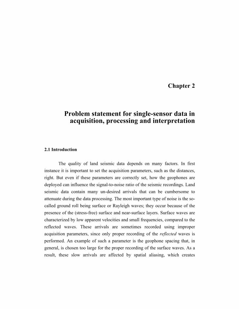
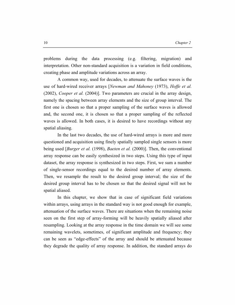
2211 One array response without and with variations Let us compute the array response using Equation 22 First we model an array with 12 identical equally spaced elements (∆x = 5 meters) The normalized amplitude spectrum and the phase spectrum of the array response are displayed in Figure 21 The amplitude spectrum is symmetrical with the Nyquist wavenumber (kN = 1 2∆x) The phase spectrum in the absence of any type of variation varies between 0 and π (see Figure 21) On the amplitude spectrum of array response we can separate three zones The first one called the pass-band zone extends from k = 0 to the first rejection notch (k1 = 1 L where L = M∆x and M is the number of array elements) The rejection notches are found using ki = i L where i = 1 2 hellip M ndash 1 the rejection notches define the wavenumbers where the amplitude spectrum of array response is zero The second zone called the aliased pass-band extends from the last rejection notch kM-1 = (M ndash 1) L to the end kM = 1 ∆x The third one known as the rejection-band extends between the pass-band and the aliased pass-band the energy present on this band should be attenuated The shape of amplitude and phase spectra displayed in Figure 21 can be distorted by the presence of different types of variations grouped into two types of variations namely the phase and amplitude variations We can model the same array response in the presence of the phase variations by mis-placing one array element using a maximum random variation of 10 from 5 metres the spacing between the others array elements is 5 meters Again we model an array with 12 elements In Figure 22 the amplitude and phase spectra are displayed in both the absence and presence of variations We notice that both spectra are affected by phase variations They look different than those obtained in the absence of variations (see Figure 22)
16 Chapter 2
Figure 21 Amplitude (left) and phase (right) spectrum of array response
Figure 22 Amplitude (left) and phase (right) spectra of array response with (solid line) and without (dashed line) phase variation for one array element
Problem statement for single-sensor data acquisition processing and interpretation 17
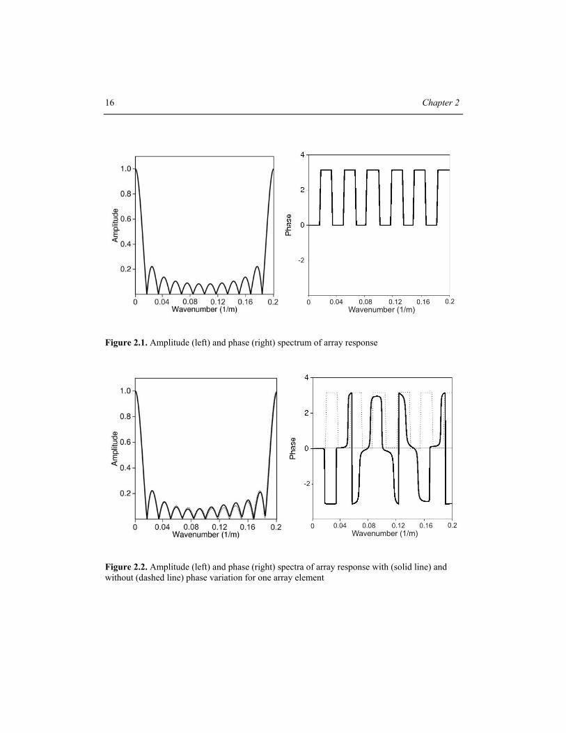
Next we model the response of an array with 12 elements in the presence of the phase variations by assuming irregular spacing between all elements instead of only one The spacing is computed using a maximum random variation of 10 from the regular spacing of 5 meters The amplitude and phase spectra of array response displayed in Figure 23 look more different than those displayed in Figure 22 The amplitude of the aliased pass-band is smaller and the amplitude spectrum has non-zero values at the rejection notches
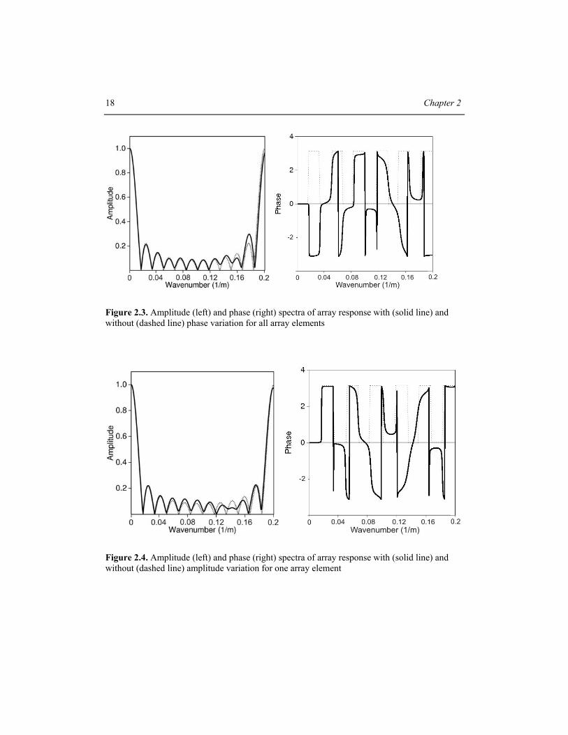
In order to analyze the effect of amplitude variations an array response we model an array with 12 elements equally spaced at 5 meters but with different weights given to each element First we assume that one array element has a random weight computed for a maximum random variation of 10 Both amplitude and phase spectra of the array response are affected by this single error (see Figure 24) The distortions observed on both spectra become stronger when all array elements instead of only one have random weights obtained for a maximum random variation of 10 (see Figure 25)
These modeling results show us that the presence of variations affects the array response depending on the magnitude of variations
18 Chapter 2
Figure 23 Amplitude (left) and phase (right) spectra of array response with (solid line) and without (dashed line) phase variation for all array elements
Figure 24 Amplitude (left) and phase (right) spectra of array response with (solid line) and without (dashed line) amplitude variation for one array element
Problem statement for single-sensor data acquisition processing and interpretation 19
Figure 25 Amplitude (left) and phase (right) spectra of array response with (solid line) and without (dashed line) amplitude variation for all array elements
2212 Multiple arrays without and with variations In the previous section we analyzed the response of one array in the absence and the presence of variations Here in order to look at the spatial characteristics we model multiple arrays using single-sensor recordings as input data The synthetic single-sensor record contains one linear event characterized by small apparent frequencies (maximum amplitude at 12 Hz) and low apparent velocity (550 ms) and one hyperbolic event characterized by high apparent frequencies (maximum amplitude at 36 Hz) and high apparent velocity (layer velocity 2000 ms) The thickness of the first layer from the geological model is 400 meters The input wavelet is the Ricker wavelet ie the second derivative of a Gaussian The spatial sampling interval is again 5 meters 80 single sensors have been used The responses of arrays with 12
20 Chapter 2
elements are synthesized and displayed in the time and frequency domain (Figure 26) no variations were used in this modeling The effect of the array is to improve the signal-to-noise ratio and conduct little distortion of the reflection wavelet Summing the elementary recordings from array elements has an effect on the reflected waveform For example the reflections coming from deep horizons are characterized by small move-out therefore the summing will result in a little distortion of the seismic wavelet (see Figure 26 right) Regarding the surface waves the effect is opposite The output of the first step from array-forming shows an effect which is due to the finiteness of an array an ldquoedge-effectrdquo two remaining wavelets with significant amplitude are seen on the time interval where the surface waves occurred on initial recordings (Figure 26 right) Looking at the amplitude (f kx)-spectrum of the single-sensor record we notice that the energy of the linear event is still significant after summing (Figure 27 right) Therefore the attenuation provided by array-forming is not at all perfect
Next we introduce phase variations in the modeling via irregular positioning of all single sensors the maximum random variation is 20 of regular spacing of 5 meters The effect of the phase variations is clear on the records displayed in both domain (Figures 28 and 29) It is known that physically the linear event is more sensitive to the irregular spacing compared with the hyperbolic event this is sustained by Figures 28 and 29 Looking at the amplitude (f kx)-spectrum we notice aliased energy that occur as dipping stripes parallel with the energy of the linear event (Figure 29) This undesired aliased energy was well attenuated after summing but the noisy energy is still significant
Problem statement for single-sensor data acquisition processing and interpretation 21
Figure 26 Synthetic single-sensor record (left) after standard array-forming (right)
Figure 27 Amplitude (f kx)-spectrum of synthetic single-sensor record (left) after standard array-forming (right)
22 Chapter 2
Figure 28 Synthetic single-sensor record with irregular positioning max random variation of 20 from 5 m (left) after standard array-forming (right)
Figure 29 Amplitude (f kx)-spectrum of synthetic single-sensor record with irregular positioning max random variation of 20 from 5 m (left) after standard array-forming (right)
Problem statement for single-sensor data acquisition processing and interpretation 23
Figure 210 Synthetic single-sensor record with amplitude variations max random variation of 20 (left) after standard array-forming (right)
Figure 211 Amplitude (f kx)-spectrum of synthetic single-sensor record with amplitude variations max random variation of 20 (left) after standard array-forming (right)
24 Chapter 2
If we introduce amplitude variations in our modeling we notice that both arrivals are affected by their presence (Figures 210 and 211) The variations were computed using a maximum random error of 20 and were introduced as weights applied to all single sensors before summing them The aliased energy an effect of these variations occurs as dipping stripes parallel with both arrivals (Figure 211) Again the array-forming could attenuate the aliased energy but the linear event still shows significant energy (Figure 211)
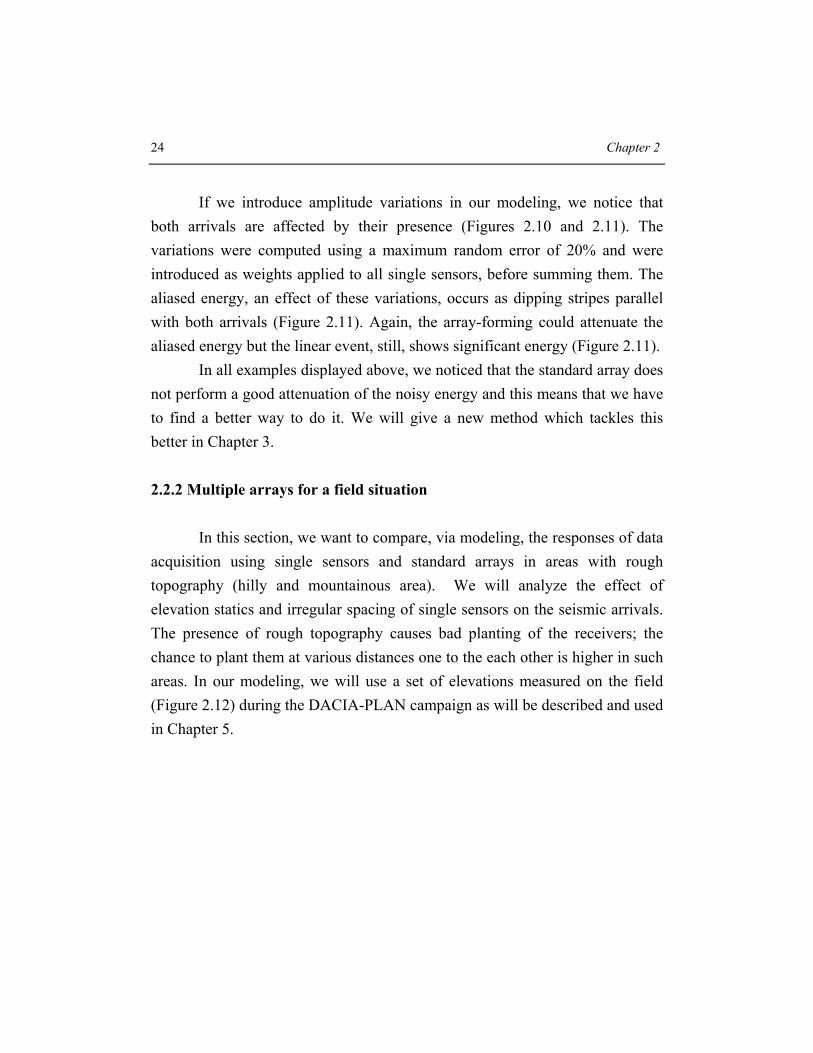
In all examples displayed above we noticed that the standard array does not perform a good attenuation of the noisy energy and this means that we have to find a better way to do it We will give a new method which tackles this better in Chapter 3 222 Multiple arrays for a field situation In this section we want to compare via modeling the responses of data acquisition using single sensors and standard arrays in areas with rough topography (hilly and mountainous area) We will analyze the effect of elevation statics and irregular spacing of single sensors on the seismic arrivals The presence of rough topography causes bad planting of the receivers the chance to plant them at various distances one to the each other is higher in such areas In our modeling we will use a set of elevations measured on the field (Figure 212) during the DACIA-PLAN campaign as will be described and used in Chapter 5
Problem statement for single-sensor data acquisition processing and interpretation 25
Figure 212 Synthetic depth model and elevation profile used in modeling
First we model 10 records with 49 single sensors spaced at 50 meters
the source spacing is 50 meters and the depth shot is 20 meters The input wavelet is a Ricker type The synthetic records contain one linear event characterized by small apparent frequencies (maximum amplitude at 12 Hz) and slow apparent velocity (600 ms) and one hyperbolic event characterized by high apparent frequencies (maximum amplitude at 42 Hz) and high apparent velocity (layer velocity 2000 ms) The thickness of the first layer is 500 meters Time sampling interval is 4 ms
It was shown before that irregular spacing between single sensors has more effect on the linear event eg surface waves (waves propagating horizontally) and statics have more effect on the reflected waves (waves
26 Chapter 2
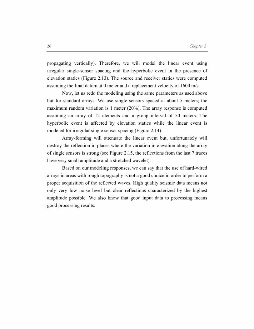
propagating vertically) Therefore we will model the linear event using irregular single-sensor spacing and the hyperbolic event in the presence of elevation statics (Figure 213) The source and receiver statics were computed assuming the final datum at 0 meter and a replacement velocity of 1600 ms
Now let us redo the modeling using the same parameters as used above but for standard arrays We use single sensors spaced at about 5 meters the maximum random variation is 1 meter (20) The array response is computed assuming an array of 12 elements and a group interval of 50 meters The hyperbolic event is affected by elevation statics while the linear event is modeled for irregular single sensor spacing (Figure 214)
Array-forming will attenuate the linear event but unfortunately will destroy the reflection in places where the variation in elevation along the array of single sensors is strong (see Figure 215 the reflections from the last 7 traces have very small amplitude and a stretched wavelet)
Based on our modeling responses we can say that the use of hard-wired arrays in areas with rough topography is not a good choice in order to perform a proper acquisition of the reflected waves High quality seismic data means not only very low noise level but clear reflections characterized by the highest amplitude possible We also know that good input data to processing means good processing results
Problem statement for single-sensor data acquisition processing and interpretation 27
Figure 213 10 synthetic records with single sensors spaced at about 50 m maximum random variation 1 m before static corrections
Figure 214 10 synthetic records based on standard array responses before static corrections
28 Chapter 2
Figure 215 One single-sensor record after adding of 12 traces and spatial resampling at 50 m before static corrections (down) and elevation profile used in modeling (up)
Problem statement for single-sensor data acquisition processing and interpretation 29
23 The use of single sensors in data processing Let us investigate the effect of single sensors and array forming in processing To this aim we process the seismic dataset modeled in the previous section in a very basic way In this way we can analyze the effectiveness of the use of single sensors or arrays for data acquisition in hilly or mountainous areas We can compare the amplitude (f kx)-spectrum of these records the CMP-gathers obtained for both datasets and at the end the time sections obtained in both situations Static corrections are applied at the beginning of the data processing (see Table 21) In this way the effect of elevation statics is nicely removed from the single-sensor data (see Figures 216 and 218 left) Things are different in case of recordings based on standard arrays Here elevation statics affect the array responses since the individual single-sensor recordings were summed before the static corrections were applied (see Figures 217 and 218 right)
Processing steps Input data 10 seismograms in SU format
24 s length Geometry yes Elevation static corrections
Final datum = 0 m Replacement velocity = 1600 ms
Velocity analysis 2000 ms NMO correction yes Stacking yes
Table 21 Synthetic data processing flow
30 Chapter 2
Figure 216 10 single-sensor records after static corrections
Figure 217 10 synthetic records based on standard array responses after static corrections
Problem statement for single-sensor data acquisition processing and interpretation 31
Figure 218 Time windowed single-sensor record (left) and one record based on array responses (right) after static corrections
Looking in detail at this effect we chose two traces from the records displayed in Figure 218 we compare the shape and amplitude of both reflections which occur at about 650 ms (Figure 219) The reflection seen on the trace selected from the single-sensor record has the maximum amplitude used in modeling and a nice shape of the Ricker wavelet The other one being on the response of an array that covered an area with important variations in elevation is characterized by very small amplitude in addition it does not show the shape of the Ricker wavelet any more
32 Chapter 2
Figure 219 Traces from a single-sensor record (dashed line) and from a record modeled using standard-arrays (solid line) after static correction have been applied
We know from modeling that array-forming affects the wavelet of the
reflections at large offset where moveout is significant especially in cases of the shallower arrivals [Panea et al (2003) Panea et al (2004)] In the presence of other types of variations eg elevation statics the array-forming will have a higher negative effect on the reflections (Figure 219)
Both datasets were sorted to the common-midpoint domain in order to obtain the required input for the velocity analysis the Normal-Moveout correction and stacking The hyperbolic events seen on the common-midpoint-gathers (CMP-gathers) differ in terms of the shape of the wavelet and amplitude (Figure 220) the CMP-gathers obtained from the single-sensor records contain wavelets with higher amplitude compared with those seen on the CMP-gathers obtained from the records based on standard array responses The NMO correction is applied in order to flatten the hyperbolic events (Figure 221)
Problem statement for single-sensor data acquisition processing and interpretation 33
Figure 220 CMP-gather from a single-sensor record (left) and from a record based on standard array response (right) before the NMO correction
Figure 221 CMP-gather from a single-sensor record (left) and from a record based on standard array response (right) after the NMO correction
34 Chapter 2
Stacking of the NMO corrected gathers will give us two different images of the time sections The time section displayed in Figure 222 is based on the single-sensor records It shows a clear reflection with high amplitude The time section displayed in Figure 223 is obtained on records based on array responses The reflection seen here looks different than the other one displayed in Figure 222 namely it is not a straight event
Figure 222 Time section obtained for single-sensor records same display parameters have been used
Problem statement for single-sensor data acquisition processing and interpretation 35
Figure 223 Time sections obtained for records based on standard array responses same display parameters have been used
24 The use of single sensors in geological interpretation In the previous sections we studied the effectiveness of the use of single sensors or conventional hard-wired arrays in the presence of surface with rough topography The quality of the processed data influences the accuracy of the image available for the geological interpretation A reliable subsurface image depends on the information contained by the stacked data and we showed that this information depends mainly on the type of acquisition Usually the geological interpretation is based on the presence of clear reflections
36 Chapter 2
characterized by the highest amplitude possible to be obtained from data processing
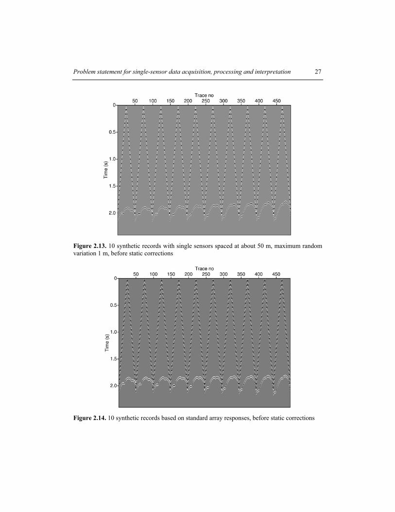
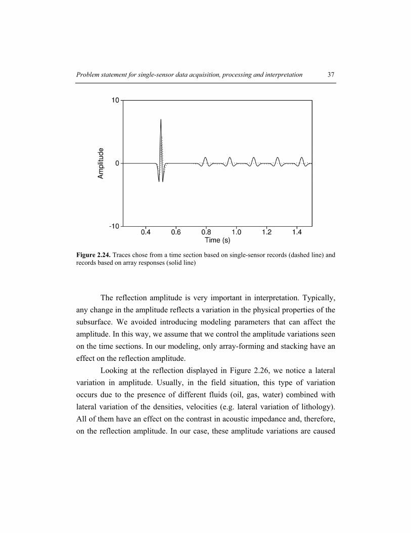
Our modeling results showed that the use of single sensors or conventional hard-wired arrays influences the shape and amplitude of the reflections For a clear image we chose and displayed one trace from a stack obtained using single-sensor recordings and the same corresponding trace from the stack computed for records based on array responses (Figure 224) Looking at these two reflections we notice that the amplitude of the reflection from the time section based on single-sensor records is almost double that of the section based on conventional hard-wired arrays responses The noisy wavelets seen on the trace chosen from the section based on single-sensor records are still significant in amplitude because we did not apply a filter during data processing We assumed that stacking would partially attenuate them On the other trace these noisy wavelets have very small amplitude as an effect of array-forming and stacking This is the advantage of using arrays in data acquisition but with the cost of reflections as we could see in our modeled field situation
Problem statement for single-sensor data acquisition processing and interpretation 37
Figure 224 Traces chose from a time section based on single-sensor records (dashed line) and records based on array responses (solid line)
The reflection amplitude is very important in interpretation Typically
any change in the amplitude reflects a variation in the physical properties of the subsurface We avoided introducing modeling parameters that can affect the amplitude In this way we assume that we control the amplitude variations seen on the time sections In our modeling only array-forming and stacking have an effect on the reflection amplitude
Looking at the reflection displayed in Figure 226 we notice a lateral variation in amplitude Usually in the field situation this type of variation occurs due to the presence of different fluids (oil gas water) combined with lateral variation of the densities velocities (eg lateral variation of lithology) All of them have an effect on the contrast in acoustic impedance and therefore on the reflection amplitude In our case these amplitude variations are caused
38 Chapter 2
by the use of conventional hard-wired arrays on a surface with rough topography In the previous sections we showed the effect of array-forming on the reflection contained by the common source- or CMP-gathers and as a consequence this effect has to occur on the stacked data
Also by comparing the images of both time sections we notice that some of the reflections seen on the section obtained using records based on conventional arrays occur at false times (see Figures 225 and 226) The geological model used in modeling contains one horizontal interface therefore the time sections should show it It does not matter if we analyze an un-migrated or migrated time section because the reflections occur at the same position in time on both The reflection seen on the time section displayed in Figure 225 shows a perfect planar horizontal limit In the other example the conventional hard-wired array case the reflection shows us a false rough horizontal limit Locally the time differences between the reflections seen on both stacks at the same position are large about tens of milliseconds
Problem statement for single-sensor data acquisition processing and interpretation 39
Figure 225 Time windowed section obtained for single-sensor records
Figure 226 Time windowed section obtained for records based on standard array responses
40 Chapter 2
Finally it is clear from these simple examples that when single-sensor data are being used it becomes possible to see events which would otherwise be missed or destroyed by data from conventional hard-wired arrays This issue is exploited in Chapter 5 where acquisition has taken place in an area with rough topography Single-sensor recordings allowed reflections to be revealed which had an impact on the geological interpretation 25 Conclusions The purpose of this chapter was to describe and analyze the main problem from data acquisition namely the attenuation of the noisy seismic arrivals The surface waves are the least desirable arrivals identified on land seismic data and therefore have to be attenuated We provided a brief description of the receiver arrays at the beginning of this chapter Also we made an introduction to the variations that can affect the array-forming responses
We modeled the response of single and multiple arrays in the absence and presence of phase and amplitude variations and we noticed that the phase variations have more significant effect on array response compared to the amplitude variations Both of them affect the amplitude and phase spectrum of the array response By modeling arrays using single-sensor records we showed that the attenuation of the surface waves is not satisfactory The remaining waves are still significant in amplitude and energy This means that we have to find another algorithm to do it (Chapter 3)
We also studied the effectiveness of using single sensors or standard arrays in areas with rough topography We showed that single sensors work better in such areas We also showed that there are field situations when the standard array responses are strongly affected by the phase variations Statics
Problem statement for single-sensor data acquisition processing and interpretation 41
can distort irreparably the shape of the reflections when using conventional arrays since they are destroyed in the array-forming Single-sensor recordings allow static corrections (or other processing as will be shown in Chapter 3) to be applied at an earlier stage in data processing
The effects of intra-array variations in the data processing were also shown It affects the CMP gathers with its associated velocity-model building Single-sensor data will be used for velocity-model estimation in Chapter 4
The effects of variation are also shown on stack level representing un-migrated time sections and show very clear the effects of intra-array variations on the reflections This will further be exploited for geological purposes in Chapter 5
42 Chapter 2
Chapter 3
The use of single sensors in data acquisition Robust Minimum Variance Distortionless
Response (MVDR) beamformer1
31 Introduction
In the last years the channel count has increased dramatically This has allowed seismic explorers to question the use of hard-wired arrays in the field Conventionally seismic arrays were needed to reduce the amount of data This reduction then put some requirements on the data the most important one being that reflections seen as the desired signal here should not be spatially aliased The nastiest arrival on land is the ground-roll that requires a much finer spatial sampling than the reflections Therefore as Vermeer (1990) has stated the array should work as a spatial antialias and resampling operator However nowadays with high channel counts fast data transfer and storage the array
1 This chapter is completely based on Panea I and Drijkoningen G 2007 The data-adaptive MVDR beamformer on seismic single sensor data paper submitted to Geophysics
44 Chapter 3
should not be considered as a hard-wire-connected array any more but as a digital array that can be treated by more sophisticated digital array processing Digital array-processing is being used in many fields A common denominator in array processing is the so-called beamformer A beamformer is a processor applied to data from an array of sensors in order to increase the signal-to-noise ratio It belongs to the class of spatial filters used in case of data where signals and noise are overlapping in frequency content but coming from different spatial directions [Van Veen and Buckley (1988) Van Veen (1991)] In a beamformer weights are applied to single array-elements to create a beam In general beamformers can be data-independent statistically optimum data-adaptive and partially data-adaptive depending on the procedure to determine the weights [Van Veen and Buckley (1988)] In case of data-independent beamformers the weights are fixed so independent of the received data For statistically optimum beamformers the weights are based on the statistics of the array The statistics of the array data are usually not known and may change over time so adaptive algorithms can be employed The data-adaptive beamformer is designed such that the response is optimal based on the data themselves Partially data-adaptive beamformers are designed in order to reduce the computational load and cost of the data-adaptive algorithms It was demonstrated that under ideal conditions the data-adaptive beamformers achieve a better signal-to-noise ratio in comparison with the conventional beamformers [Feldman and Griffiths (1994)] Also it was shown that the responses of data-adaptive beamformers are sensitive to mismatches between the presumed and actual array responses An example of possible mismatches and a solution to deal with them are given in Shahbazpanahi et al (2003) In addition the quality of data-adaptive beamformers depends on the number of analyzed data samples used in the data covariance matrix
The use of single sensors in data acquisition Minimum Variance Distortionless Response (MVDR) beamformer 45
Different types of data-adaptive beamformers have been proposed in the last two decades For the specific case of the mismatches between the presumed and actual signal-look directions algorithms have been developed like the Linearly Constrained Minimum Variance (LCMV) beamformer [see Johnson and Dudgeon (1993)] signal blocking-based algorithms [Godara (1986)] and Bayesian beamformer [Bell et al (2000)] An analysis of the performance of the MVDR beamformers in the presence of errors in signal-look directions was done by Wax and Anu (1996) Another approach in the presence of unknown arbitrary-type mismatches of the desired signal array response is proposed in the Minimum Variance Distortionless Response (MVDR) beamformer [Monzingo and Miller (1980) Vorobyov et al (2003) Jian et al (2003)]
Due to its properties the Robust MVDR beamformer presented in this chapter is suitable for dealing with seismic data since it uses matrices computed based on raw single-sensor seismic data containing both desired signal and noise Its purpose is to compute weights that will be applied to each group of recordings of single elements before their summation These weights will be different from one group to another because of the different data covariance matrices in the weight definition formula in this way we can define a proper data-adaptive beamformer 32 Design of a Robust MVDR Beamformer
In this section we will describe the Robust MVDR beamformer as derived in Shahbazpanahi et al (2003) We start with the classic MVDR beamformer definition which is based on the knowledge of two types of record one with noise (interference) and the other with a desired signal In seismic exploration the desired signal is defined as the primary reflected energy
46 Chapter 3
whereas the noise is defined as anything but primary reflected energy such as multiply reflected and refracted waves diffractions and surface waves The surface waves also known as ground roll are very dominant in land seismic data Their attenuation is difficult to define because their frequency content overlaps with that of the reflected waves Furthermore the surface wave is frequently affected by spatial aliasing arising from the receiver spacing chosen for acquisition A traditional effective way to attenuate the surface wave signal is to use an appropriate receiver array The spacing between array elements is arranged such that good reception of the surface waves is permitted This means no spatial aliasing and the size of a group interval is chosen so that the reflected waves are not spatially aliased A beamformer can be designed in combination with an array of receivers with its purpose being to compute weights based on single element recordings and to apply the weights to individual recordings before summing them into the beam It can be used to filter out the arrivals coming from other directions than that of the desired signal Our aim is to derive a beamformer such that a desired signal (reflected wave) is enhanced or at least not cancelled and interfering signals (surface wave) are attenuated or cancelled if possible
In general in seismology signals are wideband whereas in standard array processing literature many adaptive beamforming algorithms are derived under narrowband conditions so that these beamformers can be frequency independent But the design and application of a narrowband beamformer can be meaningful taking into account that the standard hard-wired arrays also frequency independent are used in reflection seismology for noise attenuation [Anstey (1986)]
The formula of the output signal of a spatial filter (beamformer or standard array) is well-known it is defined by the sum of weighted individual recordings coming from the array elements These weights can be all equal to 1
The use of single sensors in data acquisition Minimum Variance Distortionless Response (MVDR) beamformer 47
and this is the case of standard hard-wired arrays (as showed in Chapter 2) this is appropriate for the enhancement of a desired signal characterized by a small moveout including at large offsets Signals coming from other directions eg surface waves will be attenuated (as shown in Chapter 2) but sometimes not very well depending on their characteristics (eg velocity frequency)
Therefore our aim in this chapter is to take this a step further We still consider frequency-independent beamformers but design them data-adaptive such that an interfering signal (eg a surface wave) is attenuated as much as possible We first need to show under what conditions this is reasonable
In principle the data model for which this filter is applied is that of a narrowband signal For such a signal the small delay that occurs in going from one sensor to the next one can be replaced by a phase shift If so(t) is an analytic complex signal representing a narrowband signal with center frequency ω then for a sufficiently small delay τ we have
(31) os (t-τ) sje ωτminuscong o(t)
(t)
For the i-th sensor in the array we can write
(32) o i os (t-τ ) sije ωτminuscong
and for a received signal vector
do(t) = a so(t) (33)
where the vector a has as component for the i-th sensor ijia e ωτminus=
48 Chapter 3
A beamformer to cancel this signal is a beamformer whose weight vector w is orthogonal to a in that case wT do(t) = 0
If so(t) is a real narrowband signal and not complex analytic the received signal vector will be of the form
o o1 o1 o2 o2(t) s (t) s (t)= +d a a (34)
where ao1 and ao2 are two vectors that depend on the delays and center frequency but are not time-dependent In order to cancel do(t) the weight vector w provided by the beamformer has to be orthogonal to both vectors ao1 and ao2
Here the unknown vector is the weight vector w In order to estimate it we denote with Do = [do(t1) do(t2) hellip do(tN)] the data matrix that contains the recorded data sampled at the time sampling interval Next this matrix is used to compute the covariance matrix
do o ot
1 N
T=R D D (35)
where Nt is the total number of time samples The eigenvalue decomposition of Rdo will reveal that it is of rank 2
meaning that there are two nonzero eigenvalues and the others are zero with column span formed by the span of [ao1 ao2] The beamformer weight vector w can be any eigenvector corresponding to the ldquozerordquo eigenvalues or to a linear combination thereof
The required narrowband condition is
The use of single sensors in data acquisition Minimum Variance Distortionless Response (MVDR) beamformer 49
max 1BWτ (36)
where τmax is the maximum delay and BW is the bandwidth of the signal In case of wideband signals with delays that are not too large the product between the maximum delay and bandwidth could in the limit be almost equal to 1 In that case the covariance matrix will not be exactly of rank 2 therefore the ldquozerordquo eigenvalues are small but non-zero Thus the undesired signals can be attenuated but not completely canceled This fact can be used in seismology when sensors are closely spaced
In reflection seismology noise need to be separated from the reflections Noise in active seismology is mainly coherent noise On land seismic data the most important coherent noises are the surface waves since they dampen much more slowly than body waves there are considered the highest energy wave types In seismic records where seismic sensors are laid out along lines at the surface surface waves show up as linear events they also show a dispersive character and there are characterized by low frequencies (up to max 16 Hz) Since surface waves travel along the surface they have a low apparent velocity This is in complete contrast to the reflections which not only have a higher velocity but also come from below so nearly arrive vertically
The simplest data model that can approximate signal and noise in reflection seismology can be written as follows
d (t) = s (t) + n (t) (37)
where d (t) is the vector of recorded data from one array (M entries for an array with M sensors) s (t) is the part of the data that contains mostly the desired signal (reflected wave) and n (t) is the noise part of the data that contain the
50 Chapter 3
undesired signals (surface wave) We will assume that both desired and undesired signals can be considered narrowband
Let w = [w1 w2 hellip wM] T be a M times 1 weight vector to be determined based on an array with M elements The output of the beamformer is a signal y(t) = wT d(t) With Nt is the number of available time samples the output power of y(t) is estimated as
2
1
E (tN
t
y t=
= sum ) (38)
Define a matrix D that collects all sample data vectors D = [d(1) d(2) hellip d(Nt)] and define the sample covariance matrix as
t
1 N
T=R DD (39)
where R is a positive semidefinite matrix of size M times M Then E = wT R w Since d(t) is the sum of a signal and a noise term we can define the signal power at the output of the beamformer as Es = wT Rs w and the noise power as En = wT Rn w where the sample covariance matrices Rs and Rn are defined as
t
1N
Ts = s sR D D
t
1N
Tn = n nR D D (310)
where Ds Dn are M times Nt matrices that contain the desired signal and noise samples respectively
The signal-to-noise ratio denoted by SNR can be defined as
The use of single sensors in data acquisition Minimum Variance Distortionless Response (MVDR) beamformer 51
T
TSNR = s
n
w R ww R w
(311)
The aim is to select a weight vector w such that the SNR is maximized Above all we need to protect the desired signal This is guaranteed by requiring that wTRsw = 1 which means that there is no signal cancellation [Shahbazpanahi et al (2003)] Since maximizing the SNR is equal to minimizing the noise the weights for a maximal SNR are obtained from the following minimization equation
subject to min Tnw
w R w 1T =sw R w (312)
This defines the general type of Minimum Variance Distortionless Response (MVDR) beamformer The standard MVDR beamformer was proposed by Capon (1969) and more adaptive versions were proposed and studied in the following years [see Zoltowski (1988) Van Veen (1991) Raghunath and Reddy (1992) Harmanci et al (2000)] The high resolution low sidelobes and good interference suppression are some properties of the MVDR beamformer The solution to the minimization problem in Equation 312 may be found using the Lagrange multipliers method which is commonly used to find the minimum of linear functions [Shahbazpanahi et al (2003) Vorobyov et al (2003)] We define a Lagrangian function L(wλ) as a sum between the objective function wTRnw and the constraint 1 - wTRsw
(313) ( ) (1 )T TL λ λ= + minusnw w R w w R ws
52 Chapter 3
In the function L(wλ) w is an unknown optimal weight that has to be determined and used to compute the MVDR beamformer response In order to do this we calculate the gradient of the Lagrangian function as a function of weight vector w components and the Lagrange multiplier λ and equating them to zero
( )
( )
( )
( )
1 1
2 2
1 0
1 0
1 0
1 0
T T
T T
T T
M M
T T
Lw wLw w
Lw wL
λ
λ
λ
λλ λ
part part⎧ ⎡ ⎤= + minus⎪ ⎣ ⎦part part⎪part part⎪ ⎡ ⎤= + minus⎪ ⎣ ⎦part part
⎪⎪⎨⎪ part part ⎡ ⎤⎪ = + minus =⎣ ⎦part part⎪⎪part part ⎡ ⎤⎪ = + minus =⎣ ⎦part part⎪⎩
n s
n s
n s
n s
w R w w R w
w R w w R w
w R w w R w
w R w w R w
=
=
(314)
Carrying out the derivatives this result in the system
0
1 0T
λminus =⎧⎨minus =⎩
n s
s
R w R w
w R w (315)
The first equation from the system can be written as [Shahbazpanahi et al (2003) Gershman (1999)]
The use of single sensors in data acquisition Minimum Variance Distortionless Response (MVDR) beamformer 53
λ=n sR w R w
(316)
where the Lagrange multiplier λ can be viewed as a generalized eigenvalue Because Rn and Rs matrices are positive and semi-definite λ is always a real and positive number Multiplying the Equation 316 by Rn
-1 we can rewrite it as
1 1 λ
minus =n sR R w w (317)
Since λ is positive it follows that the minimum eigenvalue in Equation 316 correspond to the maximum eigenvalue in Equation 317 Based on this we can say that the optimal weight vector is given by the principal eigenvector of the product between the inverse of the noise covariance matrix Rn and the signal covariance matrix Rs [Shahbazpanahi et al (2003)]
(318) 1opt P minus= n sw R R
where P is the operator that yields the principal eigenvector of a matrix ie that corresponds to the maximal eigenvalue But the Equation 318 is applicable only up to a scaling The correct scaling is found using wTRsw = 1 Therefore we define a vector v1 = PRn
-1Rs and then the optimal weight vector is given by
54 Chapter 3
1
1 1
opts
=vw
v R v (319)
Thereafter the output of the MVDR beamformer y is obtained as follows
(320) y( ) ( )Toptt = w d t
This MVDR beamformer is difficult to apply to seismic data with the understanding that a seismic recording contains both signal and noise Separate records for these components can be derived via processing techniques or seismic modeling but their accuracy is altered and we know from previous studies that the effectiveness of the adaptive beamforming algorithms is affected by the presence of diverse errors [Shahbazpanahi et al (2003) Vorobyov et al (2003)]
To avoid using records with noise only it is desirable for seismic purposes to find another definition of the MVDR beamformer that involves the entire data set meaning records that contain both signal and noise We assume that the total signal is dominantly surface wave energy so we can replace Rn with Rd The data covariance matrix Rd is computed based on the records with signal and noise
t
1N
T=d dR D Dd (321)
where Dd is an M times Nt data matrix M is the number of array elements and Nt is the number of time samples Equation 318 can then be written as
The use of single sensors in data acquisition Minimum Variance Distortionless Response (MVDR) beamformer 55
(322) 1 opt P Pminus= congn s d sw R R R R1 minus
The replacement of the noise covariance matrix with the data covariance matrix was analyzed in the paper of Reed et al (1974) This replacement was necessary because in practical situations the noise (with or without interference) covariance matrix is unavailable It was shown that if the signal component is present in the training data this replacement decrease the performance of the beamformer whose weights are determined using Equation 322 known as the Sample Matrix Inverse beamformer [Reed et al (1974) Shahbazpanahi et al (2003) Vorobyov et al (2003)] Therefore other algorithms that define robust adaptive beamformers were proposed For example algorithms were developed in the presence of arbitrary unknown steering vector mismatches [Vorobyov et al (2003)] or in the presence of mismatches between the presumed and actual desired response [Shahbazpanahi et al (2003)]
Based on Equation 322 the optimal weights are computed using the entire data One disadvantage is introduced through the use of the signal covariance matrix Rs because it is a source of error that can degrade the quality of the MVDR beamforming response To prevent this we can introduce a matrix error ∆ in the definition of the signal covariance matrix such that it represents the possible mismatch between the presumed Rs and actual signal Ŕs covariance matrices
Ŕs = Rs + ∆ (323)
where ∆ is an M times M unknown positive semidefinite error matrix that describes the mismatch between the presumed Rs and actual Ŕs signal
56 Chapter 3
covariance matrices The norm of this matrix ∆ will be bounded by a constant ε gt 0 [Shahbazpanahi et al (2003) Vorobyov et al (2003)] The value of ε is determined by the analysis of eigenvalues obtained after the singular value decomposition of the presumed desired-signal covariance matrix and it has to be smaller than the maximum eigenvalue
The error matrix ∆ is included in the constraint equation from the MVDR beamformer definition to make it more robust to the mismatch between the presumed and actual signal array responses In addition the constraint equation is written such that to maintain a distortionless response to all possible mismatched desired signals instead of one fixed distortionless response (as in Equation 312) Therefore it is required that
wT (Rs + ∆) w ge 1 subject to || ∆ || le ε (324)
According to the assumptions published in Shahbazpanahi et al (2003) the error matrix ∆ follows as
ε= minus∆ I (325)
where I is the identity matrix The Robust MVDR beamformer problem from Equation 312 can be reformulated as
subject to min Tdw
w R w ( )T ε 1minus =sw R I w (326)
Again the solution of this problem can be determined using the method of Lagrange multipliers The optimal weight vector is given by
The use of single sensors in data acquisition Minimum Variance Distortionless Response (MVDR) beamformer 57
(327) 1 ( )opt P εminus= minusd sw R R I
Equation 327 represents the data-adaptive Robust MVDR beamformer weights not affected by the possible mismatches between the presumed and actual desired-signal covariance matrices In addition the Robust MVDR beamformer preserve the scale of the desired signal [Gershman (1999) Shahbazpanahi et al (2003) Vorobyov et al (2003)]
The design of the Robust MVDR beamformer for areal-array data (3D) is generally the same as for linear-array data (2D) The main difference between these is the size of the input data being a function of the number of receivers In the 2D case the input data are vectors of size M and for the 3D case MP where M is the number of inline and P the number of crossline single sensors Since the size of input vectors is larger the size of the signal and noise covariance matrices is greater namely MP times MP The derivation is exactly the same as for the 2D case only now the vectors contain areal- instead of linear-array data The result is then precisely as expressed in Equation 327 where the weight vector has now the size MP 33 Robust MVDR beamformer on synthetic single-sensor seismic data
In this section we show the application of the 2D and 3D Robust MVDR beamformer to synthetic data obtained by seismic modeling This was done using two modeling approaches one by simply creating a constant-amplitude linear and hyperbolic event and the other by the finite-difference method The Robust MVDR results are compared with a standard array response whose weights are fixed and equal to one The modeling with the linear and hyperbolic event was made in the presence of both phase and amplitude variations but the first consideration presented omits these
58 Chapter 3
331 Robust MVDR on 2D modeled single-sensor seismic data without variations
We first considered a response containing a linear and a hyperbolic event as shown in Figure 31 The linear event is characterized by a slow apparent velocity of 440 ms and a low frequency of 16 Hz representing for example a surface wave that is seen as ldquonoiserdquo to be attenuated The hyperbolic event is characterized by a high apparent velocity of 2000 ms and a higher frequency of 36 Hz representing a reflected wave considered to be a desired signal to be protected The depth of the reflector is 300 m The wavelet we used is a Ricker wavelet the second derivative of a Gaussian wave The first response to consider was 12 traces coming from 12 single sensors spaced 5 m apart
In seismic practice an array consists of hard-wired connected receivers so that simulation is achieved by summing the individual recordings as one output This is the first step in array forming [Hoffe et al (2002)] the second and final step is spatial resampling to a desired spacing For the robust MVDR beamformer we used the optimal weights determined from Equation 327 the data covariance matrix Rd based on 12 input traces and the signal covariance matrix Rs of the desired signal from 12 input traces containing only the reflected wave Parameter ε was determined by testing different eigenvalues smaller than the maximum eigenvalue provided by the singular value decomposition of the signal covariance matrix Rs Based on the analysis of the errors in amplitude computed using Equation 328 for different ε values for this record a good value for ε is 0001 (see Figure 32) When comparing the results
The use of single sensors in data acquisition Minimum Variance Distortionless Response (MVDR) beamformer 59
one notices that the Robust MVDR beamformer attenuates the surface waves better than standard array forming does but the desired reflected wave signal is slightly better preserved after standard array forming (see Figure 31) In addition the remaining noise seen on the Robust MVDR beamforming response is characterized by a lower frequency 4ndash6 Hz response than that seen on the standard array-forming response of about 12 Hz
The noise attenuation by standard array forming or MVDR beamforming can be quantified by defining an error between the desired response that contains only the reflected wave and the standard array-forming or MVDR beamforming response
1t
1 N
tNo s
tx n nn
e y=
= minussum y (328)
where etx is the error in amplitude computed in the time domain yo is the desired response ys is the standard array-forming or MVDR beamforming response and Nt is the total number of time samples For the example shown in Figure 31 the error etx for the standard array-forming response is 239middot10ndash4 and for the MVDR beamforming response it is 203middot10ndash4 The smaller error obtained for the MVDR response means that it is closer to the desired-array response In addition the fair comparison between all these responses is allowed because the Robust MVDR beamformer preserve the scale of the desired response [Gershman (1999) Shahbazpanahi et al (2003) Vorobyov et al (2003) Jin and Friendlander (2005)]
60 Chapter 3
Figure 31 Synthetic seismogram with 12 traces (left) after standard array-forming (right dashed line) and Robust MVDR beamforming (right solid line)
Figure 32 Error in amplitude calculated for different epsilon values (left) and the Robust MVDR weights (right) computed for ε = 0001
The use of single sensors in data acquisition Minimum Variance Distortionless Response (MVDR) beamformer 61
To look at spatial characteristics we created a larger set of single-sensor recordings where multiple arrays are formed (see Figure 33) The same modeling parameters as before are used for frequencies velocities the depth of the reflector and single-sensor spacing We used 80 single sensors and applied both the MVDR and the standard array-forming processing in order to compare the attenuation effectiveness of the slow linear event Since the goal of array forming is to spatially filter and desample the data the whole surface wave signal does not need to be removed but only the part that will be outside the new spatial band As we will show later there are situations when standard array forming does not adequately attenuate out-of-the-new-spatial-band energy which means that part of the surface waves will be spatially aliased after resampling to a larger group interval Attenuation is better achieved using the Robust MVDR adaptive beamformer We applied the Robust MVDR beamforming to this record in order to attenuate the out-of-the-new-spatial-band surface waves This algorithm was applied to an array of 12 elements The computation of the data and signal covariance matrices was done for a sliding window of 12 traces as 1ndash12 2ndash13 3ndash14 etc The traces used for the computation of the signal covariance matrix were chosen from the globally k-filtered single-sensor record that contains only the new-spatial-band energy determined for the desired group interval of 10 m Furthermore based on the singular value decomposition of the signal covariance matrix we obtained a set of eigenvalues (see Figure 34 up-left)
62 Chapter 3
Figure 33 Synthetic seismogram (up left) after standard array-forming (up right) and Robust MVDR beamforming (down) displayed in the time domain
The use of single sensors in data acquisition Minimum Variance Distortionless Response (MVDR) beamformer 63
After the analysis of the errors in amplitude computed for different ε values the value of 00005 was chosen as optimal (see Figure 34 up right) the ε value is smaller than the maximum eigenvalue obtained for each group of elementary recordings The error in amplitude is computed for the interval between the new and the old Nyquist wavenumbers
_ _
_ _
~ ~ ~ ~
1 1
1 1 f k new f k old
k old k new
N N N Ns o s o
fk f k f k f k f kf k N f k Nf k
e y y yN N
minus +
= =minus = =+
⎛ ⎞= minus +⎜ ⎟⎜ ⎟
⎝ ⎠sum sum sum sum yminus (329)
where efk is the error ỹo is the (f kx)-domain amplitude spectrum of the desired response which should be zero on these two wavenumber intervals ỹs is the (f kx)-domain amplitude spectrum of the standard array-forming or MVDR beamforming response Nk is the wavenumber sample quantity and Nf is the number of frequency samples The desired response is considered to be a record of all energy above the new Nyquist wavenumber zero Then for this ε value we computed the MVDR beamformer weights (see Figure 34 down)
The response of a standard array was also computed (see Figure 33 center) We display only the output of the first step of array forming namely the adding of traces the second step is represented by spatial resampling to a group interval that will not spatially alias the reflected waves The first step is more important than the subsequent spatial resampling because it gives us a spatially broadband picture of the noise attenuation
By comparing the responses of these two algorithms we see that the Robust MVDR beamforming achieved better out-of-the-new-spatial-band attenuation than standard array forming The remaining noise seen on the Robust MVDR beamforming response is characterized by a very low frequency of about 4ndash6 Hz compared to the original of 16 Hz In contrast the standard
64 Chapter 3
array-forming response shows us two clear linear events with the same slowness as the original one but arriving with only slightly lower frequencies than initially at about 12 Hz The (f kx)-domain amplitude spectrum of the initial record before array forming is shown in Figure 35 It can be observed that neither arrival is affected by spatial aliasing because we have not yet desampled
Figure 34 Eigenvalues (up-left) errors in amplitude for different ε values (up-right) and the Robust MVDR beamformer weights (down) determined for ε = 00005
The use of single sensors in data acquisition Minimum Variance Distortionless Response (MVDR) beamformer 65
We also notice that if we spatially resample both responses to a group interval of 10 m giving a Nyquist wavenumber of 005 mndash1 the remaining surface wave on the standard-array response would be more spatially aliased compared with the Robust MVDR beamforming response In addition if we compare the standard-array and MVDR beamformer responses with that of filtering over the wavenumber interval (- 005 005) we notice a better attenuation of the surface waves on the first two responses (see Figure 35)
The attenuation of the slow linear events can be quantified by defining the difference between the out-of-the-new-spatial-band energy in the (f kx)-domain of the desired response and of the standard array-forming or MVDR beamforming response A value of 00056 was obtained for efk in the case of standard array forming and 00050 for MVDR beamforming Based on these values we obtained better noise attenuation with MVDR beamforming If the spatial resampling were adjusted to 10 m the remaining noise contained by the standard-array response would be more spatially aliased (see Figure 35)
66 Chapter 3
Figure 35 (f kx)-amplitude spectrum of a synthetic seismogram (up left) after k-filtering (up right) standard array-forming (down left) and Robust MVDR beamforming (down right) same display parameters are taken
The use of single sensors in data acquisition Minimum Variance Distortionless Response (MVDR) beamformer 67
332 Robust MVDR on 2D modeled single-sensor seismic data with variations
The synthetic seismogram analysed above was modeled without phase
or amplitude variations The modeling parameters were chosen in order to avoid the strong spatial aliasing for both events Since field seismic records are usually affected by phase and amplitude variation it is necessary to consider their effect on the Robust MVDR beamforming response Phase variations can occur because of irregular receiver positioning variable intra-array static effects and a large lateral variation of velocity inside the receiver array Amplitude variations can occur for example due to imperfection of the geophone ground coupling
We considered phase variation in modeling the synthetic record Timing errors were introduced by mispositioning all of the receivers We again used the linear and hyperbolic event using 80 irregularly spaced single sensors A maximum variation of 20 within the receiver spacing of 5 m apart was allowed The seismogram is displayed in Figure 36 and its (f kx)-domain amplitude spectrum is shown in Figure 37 The effect of the phase variation is clear on both the (t x)- and the (f kx)-domain panels The variation generated some aliased energy seen on the (f kx)-domain amplitude spectrum observable as inclined stripes
We next applied standard array and Robust MVDR beamforming for a 12 elements array Again the computation of the data and signal covariance matrices was done for a sliding window of 12 traces as 1ndash12 2ndash13 3ndash14 etc The traces involved in the Rs computation have been chosen from a globally k-filtered record that contains only the new-spatial-band energy determined for the desired group interval of 10 m In case of the Robust MVDR beamformer the weights are computed for ε = 00004 The results are shown in Figures 36
68 Chapter 3
and 37 In observing the responses for the (t x)-domain we noticed good noise attenuation for the standard array-forming response but greater attenuation to the Robust MVDR beamforming result
The undesired striping energy of the (f kx)-domain is well attenuated by both standard array forming and MVDR beamforming (see Figure 37)
The good results obtained by Robust MVDR beamforming are supported by the quantification of the error efk determined by Equation 329 as equal to 00052 for the MVDR beamforming response For the standard array this error is 00055
The use of single sensors in data acquisition Minimum Variance Distortionless Response (MVDR) beamformer 69
Figure 36 Synthetic seismogram with irregular single-sensor spacing maximum error 20 of 5 m (up left) after standard array-forming (up right) and Robust MVDR beamforming (down)
70 Chapter 3
Figure 37 (f kx)-amplitude spectrum of synthetic seismogram with irregular single-sensor spacing maximum error 20 of 5 m (up left) after standard array-forming (up right) and Robust MVDR beamforming (down)
The use of single sensors in data acquisition Minimum Variance Distortionless Response (MVDR) beamformer 71
The effect of amplitude variation was analyzed working with synthetic records and we noticed that the effect is less than that compared to those with phase variation (see Figures 38) the effect of the amplitude variations is clear on the (f kx)-domain (see Figure 39) The aliased energy generated by this type of variation is well attenuated by the Robust MVDR beamformer whose weights were computed for ε = 00001
Also the Robust MVDR beamformer works well in the presence of groups of noisy traces (see Figure 310) Same array parameters have been used in order to compute the standard array and MVDR beamformer responses (see Figure 310) The optimal weights were computed for ε = 0001 The quantification of the error efk was done using Equation 329 being equal to 7610-8 for the MVDR beamforming response For the standard array this error is 27810-8 Therefore the Robust MVDR beamformer works better than standard array
72 Chapter 3
Figure 38 Synthetic seismogram with amplitude variation maximum error 20 (up left) after standard array-forming (up right) and Robust MVDR beamforming (down)
The use of single sensors in data acquisition Minimum Variance Distortionless Response (MVDR) beamformer 73
Figure 39 (f kx)-amplitude spectrum of synthetic seismogram with amplitude variation maximum error 20 (up left) after standard array-forming (up right) and Robust MVDR beamforming (down)
74 Chapter 3
Figure 310 Synthetic seismogram with noisy traces (left) after standard array-forming (center) and Robust MVDR beamforming (right)
The use of single sensors in data acquisition Minimum Variance Distortionless Response (MVDR) beamformer 75
Figure 311 (f kx)-amplitude spectrum of synthetic seismogram with noisy traces (left) after standard array-forming (center) and Robust MVDR beamforming (right)
76 Chapter 3
333 Robust MVDR on 2D finite-difference modeled single-sensor seismic data We have so far shown the better performance of Robust MVDR compared to standard array forming when considering the simple response of a linear and hyperbolic event To increase the complexity of the records but still have some control over the outcome we then created synthetic records using the finite-difference method based on the elastic wave equation The 2D depth model has four horizontal layers with the density and P- and S-wave velocities varying with depth These parameters are constant along the profile (Figure 312) A model shot record is displayed as Figure 313 Reflected waves are covered by dispersive surface waves at small offsets and head waves are abundant at large offsets Head waves are not well attenuated by array forming because of their high apparent velocity and frequency which are comparable with reflections
The use of single sensors in data acquisition Minimum Variance Distortionless Response (MVDR) beamformer 77
Figure 312 Depth model used for elastic finite-difference modeling
Figure 313 Synthetic seismogram (left) and its (f kx)-amplitude spectrum (right) Modeling parameters 160 single sensors with 25 meters spacing time sampling interval is 1 ms
78 Chapter 3
To prevent spatial aliasing of the reflected waves an array of 12 elements meaning an array length of 30 m was used in this case For the chosen array length the standard array-forming response did not show good noise attenuation We therefore expected that the Robust MVDR beamformer would show better out-of-the-new-spatial-band surface wave attenuation For an accurate comparison we used the same 30 m array length The application of this algorithm required the knowledge of the data covariance matrix Rd and the signal covariance matrix Rs For Rd a group of raw 12 traces was used so Rd is always a local covariance For the signal covariance a full record was used and for this the out-of-the-new-spatial-band energy was zeroed These k-filtered data were then used for the matrix Rs for all groups of 12 elementary recordings 1ndash12 2ndash13 3ndash14 and so forth given by individual sensors In this way the globally filtered record was used for the computation of all the local beamformers in that record It is important to note here that the presumed and actual desired-signal responses were different but the MVDR discussed in the design section takes account of this The matrix Rs was used for the computation of parameter ε via singular-value decomposition The optimal beamformer weights were computed for a value of ε smaller than the maximum eigenvalues obtained after singular value decomposition in our case this value was 00001 Then the optimal weights were computed for each group of single-sensor recordings In Figure 314 we display two groups of 12 single-sensor recordings chosen from the record displayed in Figure 313 that were involved in the standard-array and MVDR beamformer responses computation The first one contains the traces from the distance interval 10 ndash 375 m here the reflections are clear (see Figure 314 left) The second one contains the traces from the distance interval 40 ndash 675 m where the noise is dominant (see Figure 314 right) Using these two records as input we obtain the data covariance matrices Rd The same windows of traces were chosen from the globally
The use of single sensors in data acquisition Minimum Variance Distortionless Response (MVDR) beamformer 79
filtered record in order to compute the matrix Rs This matrix is necessary to compute the eigenvalues required by the MVDR beamformer weights computation
Figure 314 Group of traces located between 10 ndash 375 m (left) and 40 ndash 675 m (right) chosen from synthetic record displayed in Figure 313
80 Chapter 3
Figure 315 Eigenvalues for the group of traces located between 10 ndash 375 m (left) and 40 ndash 675 m (right)
We display in Figure 315 the eigenvalues determined for the group of traces placed at small (left) and large (right) distances from the shot-point Based on the analysis of these sets of eigenvalues the ε value chosen as optimal was 00001 Next the MVDR beamformer weights were calculated and applied to these group of traces before their summation If we compare the weights obtained for these two groups of 12 traces records we notice that they are almost constant along the array in cases where the desired signal is dominant or show a significant variation in cases where the noise is dominant (see Figure 316)
Looking at the Robust MVDR beamforming response displayed in Figure 317a we note appreciable attenuation of the out-of-the-new-spatial-band surface waves with clear reflected waves at larger offsets than in the initial record (see Figure 313)
As expected the refracted waves are still high in amplitude but the same result is seen for the standard array-forming response Significantly the out-of-
The use of single sensors in data acquisition Minimum Variance Distortionless Response (MVDR) beamformer 81
the-new-spatial-band surface waves are not greatly attenuated after standard array forming (see Figure 317a) Furthermore when considering the (f kx)-domain representation as shown in Figure 317b the Robust MVDR result appears more positive
Figure 316 Robust MVDR beamformer weights for the group of traces located between 10 ndash 375 m (up left) and 40 ndash 675 m (up right) and the error in amplitude for different ε values (down)
82 Chapter 3
If we attempted the second step of spatial resampling for example to a group interval of 10 m meaning a Nyquist wavenumber of 005 mndash1 the remaining surface waves would be spatially aliased in the standard-array case much less so for MVDR (see Figure 317b)
Figure 317a Synthetic seismogram after standard array-forming (left) and Robust MVDR beamforming (right) displayed in the time domain
The use of single sensors in data acquisition Minimum Variance Distortionless Response (MVDR) beamformer 83
Figure 317b (f kx)-amplitude spectrum of synthetic seismogram after standard array-forming (left) and Robust MVDR beamforming (right) same display parameters are taken
Since the (f kx)-domain amplitude spectrum of the Robust MVDR beamformer shows better out-of-the-new-spatial-band attenuation its spatial resampling would give a record with surface waves scarcely spatially aliased
As a quantification of noise attenuation efficacy by the Robust MVDR beamformer error efk based on Equation 329 is 00048 for the standard-array response and 00030 for the MVDR beamforming response so the MVDR result is better
84 Chapter 3
334 Robust MVDR on 3D finite-difference modeled single-sensor seismic data
In the previous account we analyzed the effect of the Robust MVDR beamformer on 2D synthetic seismic data We noticed that the surface waves were well attenuated even in the presence of phase and amplitude variation Considering that we wish to analyze a partial-3D field data set we must look at the effect of the 3D MVDR beamformer on 3D synthetic data We modeled a synthetic data set using the elastic finite difference code The 3D depth model used is an extension of the 2D model shown in Figure 312
The synthetic record was modeled using a strip of five lines of single sensors spaced at 5 m in the inline and crossline directions (see Figure 318) the source was located on the third line The array with 6 inline and 5 crossline elements was chosen to prevent the spatial aliasing of the arrivals contained by the modeled record The group interval was 10 m and the beamformer weights were computed with a value of ε = 0001 The desired signal is a record showing zero out-of-the-new-spatial-band energy consequently we filtered all the traces in the global record The covariance matrix of the desired signal involved in the weight definition is then the presumed signal covariance matrix The actual signal covariance matrix of the local array was slightly different but our Robust MVDR takes account of this The data covariance matrix was computed using the synthetic record that contains desired signal and noise to this end we only used the raw traces that belong to the local array
Looking at the Robust MVDR beamforming response displayed in the (t x)- and (f kx)-domains in Figures 319a and 319b we notice a greater out-of-the-new-spatial-band energy attenuation for the MVDR compared to the result for standard array forming
The use of single sensors in data acquisition Minimum Variance Distortionless Response (MVDR) beamformer 85
Figure 318 Synthetic record with 5 seismograms for 80 single-sensors with 5 meters spacing (inline direction) Depth model parameters as defined in Figure 312
86 Chapter 3
Figure 319a Standard array-forming (left) and Robust MVDR beamforming (right) responses for arrays with 6 times 5 elements for finite-difference modeled data Depth model parameters as defined in Figure 312
The use of single sensors in data acquisition Minimum Variance Distortionless Response (MVDR) beamformer 87
Figure 319b (f kx)-amplitude spectrum of standard array-forming (left) and Robust MVDR beamforming (right) responses for arrays with 6 times 5 elements for finite-difference modeled data Depth model parameters as defined in Figure 312
The remaining surface waves are clear on the standard array-forming response displayed in the (t x)- and (f kx)-domains (see Figures 319a and 319b) The same procedure as for the 2D case was followed here in order to quantify the noise attenuation performed by the 3D MVDR beamformer A value of 00149 was obtained for error efk with the 3D MVDR beamformer which is much less than 00630 obtained for the standard array This indicates that the MVDR beamformer gives a result much closer to the desired array response compared with standard array forming
88 Chapter 3
34 Robust MVDR beamformer on single-sensor field data
In this section we consider the 2D and 3D MVDR beamformer used on single-sensor field data These data were recorded using a strip of five lines of single sensors spaced at 5 m in the inline and crossline direction The seismic energy was generated with dynamite the source spacing as 20 m and the source locations were only on the central line of the single sensors One purpose of the project whose records are used in this section was to apply the MVDR technique and compare it with standard array forming In this particular case the field data were affected by variation in the amplitude and phase because data acquisition took place in a hilly area with a notable elevation difference along one receiver array (see Figure 320) In addition lateral velocity variation is known in this area especially in the shallower layers Amplitude variation occurred because of soil conditions that locally did not provide good soil-geophone coupling
Figure 320 Elevation variations along the seismic profile of field data
The use of single sensors in data acquisition Minimum Variance Distortionless Response (MVDR) beamformer 89
341 Robust MVDR on 2D single-sensor field data
We first applied the beamformer to a one shot record (see Figure 321a) Looking at the two time responses we notice that the remaining surface waves are easier to identify on the standard array-forming response than on the Robust MVDR beamforming response (see Figure 321a) We used an array with 12 elements If we compare the standard array-forming with the MVDR beamforming response in the (f kx)-domain as depicted in Figure 321b we notice clear aliased energy to be concentrated around a wavenumber of 005 mndash
1 and a frequency of 10 Hz on the standard array-forming response Conversely this aliased energy is seen to be more attenuated after MVDR beamforming (see Figure 321b) The parameter ε required for the computation of the MVDR weights was determined using the singular-value decomposition of the signal covariance matrix Rs this matrix was again computed using a filtered version of the analyzed record over the interval (ndash kNnew + kNnew) obtained for the 10 m group interval The second matrix involved in the weight computation is the data covariance matrix Rx and it was computed based on the raw single-sensor records The best out-of-the-new-spatial-band energy attenuation obtained was for ε = 002 To quantify the effectiveness of noise attenuation performed by the 2D Robust MVDR beamformer using Equation 329 we noted ef k = 00088 for the MVDR beamforming response and the higher value of efk = 00118 for the standard-array response
90 Chapter 3
Figure 321a Field record (left) after standard array-forming (center) and Robust MVDR beamforming (right) displayed in the time domain
The use of single sensors in data acquisition Minimum Variance Distortionless Response (MVDR) beamformer 91
Figure 321b (f kx)-amplitude spectrum of field record (left) after 2D standard array-forming (center) and 2D Robust MVDR beamforming (right) same display parameters are taken
92 Chapter 3
Figure 322 Field record (up-left) after standard array-forming (up-right) and Robust MVDR beamforming (down) displayed in the time domain
The use of single sensors in data acquisition Minimum Variance Distortionless Response (MVDR) beamformer 93
Also the Robust MVDR beamformer can attenuate the noisy traces that do not carry seismic information In this example one noisy trace can appear multiplied on the standard-array response while its presence is completely attenuation on the MVDR beamformer response (see Figure 322)
342 Robust MVDR on partial-3D single-sensor field data
We next considered a partial-3D shot record with the 3D Robust MVDR beamformer (see Figure 323) In this case we applied the MVDR algorithm for an array with 12 inline times 5 crossline traces The standard array-forming and MVDR beamforming responses are displayed in Figure 324a By comparing these two results we notice better out-of-the-new-spatial-band energy attenuation by the MVDR algorithm (see Figure 324a) The size of the new spatial band depends on the value of the group interval here 10 m Looking at both responses displayed in the (f kx)-domain (see Figure 324b) we can clearly see that the standard array-forming response has a remaining surface wave energy concentrated around a wavenumber of 005 mndash1 and a frequency of 10 Hz whereas the MVDR beamforming response is much less The error in amplitude efk shows a value of 00142 for the MVDR beamforming and efk = 00158 for the standard array-forming response
94 Chapter 3
Figure 323 One record of field data
The use of single sensors in data acquisition Minimum Variance Distortionless Response (MVDR) beamformer 95
Figure 324a Field record after 3D standard array-forming (left) and 3D Robust MVDR beamforming (right) displayed in the time domain
96 Chapter 3
Figure 324b (f kx)-amplitude spectrum of the field record after standard array-forming (left) and Robust MVDR beamforming (right) same display parameters are taken
343 Data processing of the 3D standard array-forming and 3D Robust MVDR beamforming responses
The effectiveness of the noise attenuation performed by the Robust MVDR algorithm can also be seen on stacked sections A usual way to attenuate the noise is to stack the seismic data in the CMP (common midpoint) domain after the normal moveout corrections When we use a standard array to record the seismic data the noise is first attenuated by this array and then by the CMP stacking Thus we use two ways to increase the signal-to-noise ratio apart from other techniques such as filtering
The use of single sensors in data acquisition Minimum Variance Distortionless Response (MVDR) beamformer 97
We have so far demonstrated that only on shot records does the MVDR algorithm result in better surface-wave attenuation than standard array forming The analyzed data set contains 157 records each representing five seismograms with 160 traces spaced at 5 m This data set was introduced to 3D standard array forming and 3D Robust MVDR beamforming The results of the two approaches were further processed using the same flow to allow for comparison (see Table 31) Static corrections were applied first using a replacement velocity of 1750 ms for a final datum of + 450 m above sea level The remaining surface waves were further eliminated using an f-k filter f-x deconvolution and a band-pass frequency filter of 20ndash24ndash64ndash70 Hz The second step of array forming namely the resampling to a new group interval of 10 m was next done Amplitude equalization was achieved using automatic gain control for a window of 300 ms Top mute was applied to remove the first arrivals and the advance noise The CMP stacking of seismic data used a 2D velocity model provided by the velocity analysis
When we compare the two time sections obtained in this way we notice an improvement in the continuity of some reflectors all over the section when applying the 3D MVDR responses (see Figure 325) For example looking on the left side of both time sections the continuity of those reflections located between 05 s and 1 s is stronger These same reflections are weaker and discontinuous with the 3D standard array-forming result (see Figure 326) Both sides of the time sections show high reflectivity This is due partially to the favorable signal-to-noise ratio that characterizes the recordings and partially to the 3D robust MVDR beamforming algorithm The central part of the section has a very low signal-to- noise ratio because of the low quality of input data this is a result of the field conditions of rugged topography and unconsolidated soil giving a bad geophone coupling Use of the 3D beamformer enhanced the signal-to-noise ratio of the analyzed recordings
98 Chapter 3
Processing steps
Parameters
Input seismic data 2 s trace length
157 shots
Geometry 2D land geometry
Static corrections Replacement velocity = 1750 ms
Final datum = + 450 masl
Desampling in time 2 ms
Trace muting Top (first arrivals and noise before)
Automatic Gain Control 300 ms
f-k filter Accept fan polygon
Trace muting Top (remaining noise)
Automatic Gain Control 300 ms
Band-pass frequency filtering Zero phase frequency
20ndash24ndash64ndash70 Hz
Notch filter 50 Hz window of 4 Hz
f-x Deconvolution Wiener Levinson 500 ms 20ndash70 Hz
Automatic Gain Control 500 ms
Spatial resampling Group interval of 10 m
Velocity analysis Yes
NMO corrections Yes
Stacking Yes
Table 31 Data processing steps of field data set and parameters used
The use of single sensors in data acquisition Minimum Variance Distortionless Response (MVDR) beamformer 99
Figure 325 Time section of field data set based on 3D Robust MVDR beamforming
Figure 326 Time section of field data set based on 3D standard array-forming
100 Chapter 3
Figure 327 Windowed time sections based on 3D robust Robust MVDR beamforming (left) and 3D standard array-forming (right)
The amplitude of some reflectors was higher after Robust MVDR beamforming than after standard array forming See for example the group of reflectors located between 1500ndash2000 m on the time section at the time interval of 16ndash19 s (see Figure 325) Some shallow reflectors also appear to be more continuous (see Figure 327) 35 Conclusions
The Robust MVDR beamformer is an algorithm proposed to attenuate undesired energy located within the new spatial band defined by the value of the group interval Modeling results show that it can be successfully used for seismic data in combination with single-sensor recordings The application of 2D or 3D Robust MVDR beamforming to synthetic data showed noise attenuation appreciably better than that provided by either 2D or 3D standard array forming Qualitative and quantitative estimation of this attenuation made by comparing the responses displayed in the (t x)- and (f kx)-domains support
The use of single sensors in data acquisition Minimum Variance Distortionless Response (MVDR) beamformer 101
this observation The error shows smaller values for Robust MVDR beamforming in all cases for both synthetic and field records which means that this algorithm provides us with more acceptable responses than those obtained by alternative processing
Application of the 3D Robust MVDR beamformer to post-stack data enhanced the signal-to-noise ratio more than standard array forming including in those areas where the SNR is very low We notice more continuous reflections and higher amplitudes in the time section based on the Robust MVDR responses In addition the Robust MVDR algorithm works well with data that have a very low signal-to-noise ratio which is encouraging because land seismic data often have this characteristic
102 Chapter 3
Chapter 4
The use of single sensors in processing stereotomography2
41 Introduction
In this chapter the use of densely spaced single sensors in processing is
exploited In the previous chapter the effect of two types of algorithms was analyzed regarding the noise attenuation (a source-generated coherent noise ie ground-roll) Here we do not do any (in-line) array-forming but treat the dataset as a single-sensor dataset to be processed Since it is a single-sensor dataset the output stacked section contains more traces than the section that
2 This chapter is based on Panea I Landa E Drijkoningen GG Baina R 2005 Imaging using post-stack stereotomography in areas with low signal-to-noise ratio Journal of the Balkan Geophysical Society Vol 8(4) pp 161-174
104 Chapter 4
would have been obtained if the array data was used Actually the analysis and processing we are going to discuss in this chapter would not have been possible at all if we would have used array data because then there would have been too few traces in the final section On top of that since the topography of the area was quite substantial arrays would have destroyed part of the desired signal (reflected waves) due to static errors It is obvious for such areas that single-sensor data allows tackling these problems
The processing step we are going to discuss in this chapter is stereotomography Stereotomography is a method that determines a macro-velocity model from seismic reflection data [Billette and Lambareacute (1998)] In its original form it was based on the automatic picking of locally coherent events on pre-stack data (common shot offset midpoint and receiver gathers) Since the automatic picking on pre-stack data characterized by low signal-to-noise ratios does not provide reliable picks the resulting velocity model can be far away from the true model Therefore Lavaud et al (2004) proposed a modification to stereotomography based on the automatic picking of local coherent events on post-stack data namely on a Common-Reflection-Surface (CRS) stack We will use this approach in this chapter Next the velocity model is determined based on the inversion of the travel-times picked on the CRS stack The combination of these two steps is known as ldquopost-stack stereotomographyrdquo
The post-stack stereotomography was applied with good results on synthetic seismic data and marine seismic dataset [Lavaud Baina and Landa (2004) Lambareacute Alerini and Podvin (2004)] In addition the post-stack travel-time picking seems to be a robust and reliable procedure commonly used in seismic interpretation [Lavaud et al (2004)] This method belongs to the slope tomography methods proposed during the last decade [Billette and Lambareacute (1998) Chauris Noble Lambareacute and Podvin (2002) Duvenek and Hubral
The use of single sensors in processing stereotomography 105
(2002)] The optimal wavefront parameters are obtained during the generation of the CRS stack [Jaumlger Mann Houmlcht and Hubral (2001)] The stereotomography has been implemented in 2D [Billette Le Begat Podvin and Lambareacute (2003)] and 3D [Chalard Podvin Le Begat Berthet and David (2002)]
In this chapter we focus on a field dataset with a low signal-to-noise ratio this dataset was recorded using single sensors Because of its low signal-to-noise ratio the velocity analysis performed on the CMP gathers with the standard procedure did not provide a very reliable 2D velocity model Most of the CMP gathers were avoided during this analysis because of their low desired signal level Next the depth migration does not run well because the interval-velocity model derived from the conversion of the stacking velocities is not good enough Knowing that the signal-to-noise ratio can be improved also by stacking of the data it seems that the post-stack stereotomography can be used with good results In addition there is a possibility to verify the accuracy of the velocity model by a Common-Image-Gathers (CIG) analysis during the migration step
In this chapter we first briefly describe the principles of the stereotmography method based on the CRS-stack approach Then we introduce the single-sensor dataset used for analysis and discuss the two approaches in two separate sections In this way we compare the standard CMP-based approach with the CRS-stereo-tomography approach Although the algorithm used is 2D some 3D effects have been used too Cross-line arrays would in theory help increasing the signal-to-noise ratio even more Via a single-sensor field dataset we will also show that the results are even improving when the data is stacked in the cross-line direction
106 Chapter 4
42 Background to the post-stack stereotomography
We start with a short description of the stereotomography method also known as the ldquopre-stack stereotomographyrdquo [Billette and Lambareacute (1998)] Stereotomography is a method used for estimating velocity macro-model from seismic reflection data and belongs to the slope tomographic methods
The velocity model is obtained by the inversion of the travel-times picked on locally coherent events in a gather of traces (for example common source common receiver common offset common CDP gathers) In addition two slopes are determined for each event the first one in the common source gather and the second one in the common receiver gather These slopes correspond to the horizontal component of the slowness vectors according to the ray theory [Billette and Lambareacute (1998)] Each locally coherent event picked on a given trace is described by source and receiver positions (S = (xS zS) and R = (xR zR)) a two-way travel-time tSR and two local slopes (pSx = ∆t∆xp and pRx = ∆t∆xp) this information define the ldquoobservedrdquo data part of stereotomography noted with 1[( ) ] eNr
i Sx Rx SRd S R p p t i i== for Ne picked events The source and receiver positions are known from the navigation files
obtained in the field The two-way traveltime is read on the data The slope is defined as the tangent of a coherent event measured from pre-stack seismic trace gathers [Billette et al (2003)] In a 2D trace gather (can be a common source common receiver common offset common CMP gather) we can measure the slope px of a given coherent event at a given receiver or source location (see Figure 41) On a common source gather or common receiver gather the local slope of a reflected event provides a direct estimation of the horizontal component of the slowness vector Next these slopes can be used to reconstruct the path to the reflecting diffracting point X starting from the surface This reconstruction requires also an initial velocity model Based on
The use of single sensors in processing stereotomography 107
this information the rays are traced down from the surface until a point where they should intersect if the velocity model is good In this case the picked travel-time has to be equal with the sum of the two one-way travel-times computed for both rays that cross each other If the picked event is a primary reflection or diffraction it can be associated with a reflecting diffracting point X This point X is localized at the intersection of the two ray segments the first one goes from the source point S down to the reflecting diffracting point X
and the second one goes from the reflecting diffracting point X up to the receiver R A ray segment means a part from a ray trajectory completely defined by a starting point and an ending point the initial or final direction and the travel-time
XS rarr
RX rarr
Figure 41 The slope on a common-source gather and the slope in ray theory [after Billette and Lambareacute (1998)]
Two conditions have to be satisfied by these rays namely they have to cross each other at their ending point and they have to fit the data in positions
108 Chapter 4
slopes and two-way travel-times These conditions also known as boundary conditions are not entirely satisfied in case of an incorrect velocity model therefore one of them has to be variable Three cases were proposed here
In the first one none of the boundary conditions are fixed which means that the ray segments do not have to join each other in depth or fit the data at the surface (see Figure 42) This is the general case of the slope tomographic methods here the velocity and ray segments update until all the boundary conditions fit the data and the ray segments join each other at a point in depth
The second case is found in the Controlled Directional Reception (CDR) method [Sword (1987)] It assumes the surface boundary condition fixed meaning that the upper extremities of the two ray segments have to fit the data at the surface the lower extremities do not have to fit in depth (see Figure 43)
In the last case the crossing point is fixed (the rays have to cross each other at the deepest point) and the surface boundary condition is relaxed (both rays do not fit the data at the surface) This is the assumption take it into account in stereotomography (see Figure 44)
Figure 42 No boundary condition is fixed ray segments do not have to join each other in depth or fit the data at the surface [after Billette and Lambareacute (1998)]
The use of single sensors in processing stereotomography 109
Figure 43 Surface boundary conditions are fixed (the upper extremities of the two ray segments have to fit with data at the surface) their other extremities do not have to fit in depth [after Billette and Lambareacute (1998)]
Figure 44 Crossing-point is fixed the two ray segments do not have to fit the data at the surface [after Billette and Lambareacute (1998)]
Stereotomography characterizes each picked event by a pair of ray segments that terminate at the same point in depth (called X) These ray segments propagate upwards from the point X into an initial velocity model with known directions to the source and receiver and two one-way travel-times this information define the so-called model part m of stereotomography
Based on the model part analysis a ldquocomputedrdquo dataset is obtained d S
1 1j j=[[( ) ] [ ] ]eN JS R S R i im X T T Cβ β ==
1[( ) ] eNci sx rx SR i iR p p T == (see Figure 45)
110 Chapter 4
Figure 45 Calculated data are obtained from an initial model m they do not match
real data [after Billette and Lambareacute (1998)]
cid
rid
The travel-times and local slopes contained by the ldquoobservedrdquo dataset are determined by automatic picking The stereotomographic picking can
be done in the time domain Also Chauris et al (2002) demonstrated that it can be done in the depth migrated domain because of higher signal-to-noise ratio better coverage of the model and easier quality control of the picks The second step after the automatic picking is the visual check of the picks and manual correction [Alerini et al (2003)] Lambareacute et al (2003) proposed a picks selection based on the statistical properties of the population of stereotomographic picks this is done based on an interactive visualization of the picks as a function of thresholds The outlier pick in terms of slopes equivalent model parameters picks with too small coherency or energy are eliminated [Lambareacute et al (2004)] The following control parameters are used
rid
The use of single sensors in processing stereotomography 111
in order to increase the accuracy of automatic picking the distance between analyzed traces the time sampling increment the width of Hamming window a threshold on the semblance value a threshold on the product of the semblances from common shot common receiver and common offset gathers
As is written above the model part of stereotomography m is represented by a velocity macro-model Cm and a set of pairs of ray segments parameters associated with each picked event ( for N1[( ) ] eN
S R S R i iX T Tβ β = e locally coherent picked events) The initial velocity model is considered homogeneous and described by a number of nodes The location of the reflecting diffracting point X is obtained during the picking procedure The angles are computed based on simple geometrical considerations assuming a homogeneous medium Each of the two one-way travel-time pairs is set to half of the corresponding two-way travel-time picked from the data Initially the ray paths do not reach the surface in the observed positions their correction is made assuming the initial model correct and varying the ray segments parameters [Billette et al (2003)] A first version of the velocity model is obtained by a stereotomographic inversion that consists in fitting all the picked data with the data calculated by ray-tracing [Chalard et al (2002)] Next all picks are used to upgrade simultaneously the associated rays and velocity perturbation having as result the final velocity model
More accurate picks are obtained if we use stacked data because the noise level is lower on the stacked data compared to that one from pre-stack data The so-called post-stack stereotomography uses picked travel-times on the Common-Reflection-Surface stack so the post-stack domain The CRS stack gives an accurate zero-offset approximation of the seismic section in addition the procedure used to generate the CRS stack is also used to compute the wavefront parameters for each CMP position and time sample (emergence angle of the zero-offset ray and two radii of wavefront curvatures RN and RNIP)
112 Chapter 4
These three parameters are associated with two hypothetical waves namely the normal wave (N) and the normal-incidence-point wave (NIP) The N and NIP waves also known as eigenwaves result from two hypothetical experiments where a point (diffractor-like) and a reflector are the secondary source in the subsurface For example Figure 46 shows a model with three homogeneous layers for these two types of cases The NIP wave is obtained by placing a point source on a reflector (see Figure 46 left) so like a point-diffractor and the N wave is obtained after a simultaneous excitation along a reflector (see Figure 46 right) so like an exploding reflector In the vicinity of a point from the acquisition line x0 both wavefronts can be approximated by circles with radii of curvature RNIP
and RN respectively [Jaumlger et al (2001)]
The use of single sensors in processing stereotomography 113
Figure 46 NIP wave for a point source at R position (up) and N wave for an exploding reflector at R position (down) [after Jaumlger et al (2001)]
The computing of the CRS stack does not depend on a macro-velocity model [Jaumlger et al (2001)] as opposed to the CMP stack The CRS-stacking operator is defined as
114 Chapter 4
( ) ( )22 2 202 0
0 0 00 0
2sin 2 cos( ) cmpCRS cmp
N NI
x xt ht x h t x xR R
β βν ν
⎛ ⎞minus⎛ ⎞ ⎜ ⎟= + minus + +⎜ ⎟ ⎜ ⎟⎝ ⎠ ⎝ ⎠P
(41)
where x0 is the output position xCMP is the position of midpoint between source and receiver (= (xR + xS)2) h is the half offset (= (xR - xS)2) v0 is the near surface velocity t0 is the zero-offset two-way traveltime
The three parameters (β RN and RNIP) define the stacking surface associated to the zero-offset traveltime t0 If the point P0 = (x0 t0) is known all we need is the near-surface velocity v0 [Jaumlger et al (2001)] This parameter is assumed to be known eg from other seismic studies performed in the studied area
It has been shown that a CRS stack improves the signal-to-noise ratio and provides a better continuity of reflectors this statement is based on synthetic and field data analysis Each trace from the CRS stack is obtained by summing the traces from a super CMP gather so that a better noise attenuation is achieved In addition it is known that the procedure used to compute the CRS stack is also used to extract the information from the pre-stack data about the wavefront parameters these parameters are determined for each point P0 of the zero-offset section [Jaumlger et al (2001)]
Once we have the CRS stack an automatic travel-time picking is performed as a first step of the post-stack stereotomography method here only the locally coherent events are picked The 2D velocity model is obtained after an iterative inversion process of the picked travel-times it is a smooth model and contains interval velocities as a function of depth Then the velocity model will be used for the pre-stack depth migration of the stacked seismic data
The use of single sensors in processing stereotomography 115
43 Application of post-stack stereotomography on a single-sensors seismic dataset recorded in a low signal-to-noise area 431 Seismic dataset Acquisition and pre-processing
The post-stack stereotomography method is applied to a shallow land seismic dataset in order to get a more accurate velocity model necessary for the depth migration The depth migrated section should show us a good depth image of the studied area namely the proper positioning of the reflectors in depth Before using this method the land seismic data need a pre-processing in order to obtain common-midpoint (CMP) gathers having a signal-to-noise ratio as high as possible The shallow seismic reflection dataset was recorded as a part of larger seismic survey (see Figure 47) Dynamite was used as a source and the seismic information was recorded using vertical-component geophones (see Table 41 for the data acquisition parameters) In general the quality of the seismic records is better toward the profile edges clear reflectors can be seen even on the raw seismograms The static effects are important they can be identified on the raw seismograms The elevation values vary along the seismic profile the spread of the receivers for the first shot (1 ndash 160) covered 800 m and the maximum difference in elevation is 110 m (see Figure 48)
116 Chapter 4
Figure 47 Topographic map of the studied area (Dumitresti-Ramnicu Sarat)
Parameters
Receiver spacing 5 m Receiver number 160 Source spacing 20 m Source type dynamite Source size 200 g Source depth 2 m Sampling time interval 1 ms Time length 4 s
Table 41 Data acquisition parameters
The use of single sensors in processing stereotomography 117
Figure 48 Elevation variation along the seismic reflection profile
It is known from previous seismic studies that there are important near-
surface velocity variations Together with the elevation effect they create statics that have to be extracted from the recorded data A final datum of + 450 m has been chosen in order to compute the static corrections and a replacement velocity equal with 1750 ms has been used
The signal-to-noise ratio of the seismic data is enhanced by different filtering techniques (band-pass f-k f-x Deconvolution) First we tried to remove the ground-roll from the analyzed dataset by applying the f-k filter followed by the other filters to eliminate the remaining noise (see Table 42 for the pre-processing steps) The top mute is used to remove refracted waves and noise before the first arrivals Some of the very noisy traces were zeroed The automatic gain control is used to normalize the energy along the traces
118 Chapter 4
Figure 49 Raw seismograms 2025 (up left) 2120 (up right) and 2193 (down) (their positions on the seismic profile are shown in Figure 47)
The use of single sensors in processing stereotomography 119
Figure 410 Pre-processed seismograms with static corrections applied 2025 (left) 2120 (center) and 2193 (right) (their positions on the seismic profile are shown in Figure 47)
120 Chapter 4
The full pre-processing flow is given in Table 42 In Figure 49 we display three of the most representative shots from the entire dataset and the results after pre-processing in Figure 410 The signal-to-noise ratio of these seismograms is indeed enhanced
Pre-processing steps Parameters
Input seismic data 2 s trace length 157 shots
Geometry 2D land geometry Static corrections Replacement veloc = 1750 ms
Final datum = + 450 m Desampling in time 2 ms Trace muting Top (first arrivals and noise
before them) Trace KillReverse Kill (very noisy traces) Automaic Gain Control 300 ms f-k filter Accept fan polygon Trace muting Top (remaining noise) Automatic Gain Control 300 ms Band-pass frequency filtering
Zero phase frequency 20 ndash 24 ndash 64 ndash 72 Hz Notch filter 50 Hz window 4 Hz
f-x Deconvolution Wiener Levinson 500 ms 20 ndash 70 Hz
2D Spatial Filtering Convolutional method Trace Muting Top (remaining noise) Trace Muting Bottom (remaining noise) Automatic Gain Control 300 ms
Table 42 Data pre-processing flow
The use of single sensors in processing stereotomography 121
432 Imaging using standard CMP-based approach
The standard velocity analysis was performed on the CMPs obtained from the pre-processed data (see Figure 411) Then the 2D velocity model was used to obtain the un-migrated section (the CMP stack) The CMP stack is displayed in Figure 412 As expected the reflectivity between 0 ndash 1 km and 22 - 32 km is higher compared to that one seen on 15 ndash 22 km The reflections are clear continuous on great distances and characterized by high amplitude The CMP stack shows us a simple geological structure with important geological interfaces characterized by a high contrast of acoustic impedance and represented by clear and high amplitude reflectors The poor quality of the stacked data on the central part of the CMP stack can be a result of many factors namely the low signal-to-noise ratio of the input data the presence of the surface waves rough topography and near-surface effects The elimination by filtering of the surface waves identified on a group of seismograms was difficult even using the f-k filter Also the elevation and near-surface effects are very important on this segment of the seismic profile due to the field conditions (forest frequent elevation variations on small horizontal direction with large amplitude lateral variations of the near-surface velocities)
We expect to obtain a higher quality of this segment of the seismic profile after the post-stack stereotomography based on the procedure used to compute the CRS stack and the 2D velocity model
122 Chapter 4
Figure 411 2D velocity model based on CMP velocity analysis
433 Imaging using post-stack stereotomography
The CRS stack is a simulation of the zero-offset stack The only difference between a CMP and CRS stack is the aperture used for stacking the size of this aperture defines the number of the CMP gathers combined during stacking (multiple of CMP gathers in case of the CRS stack) The reflectivity of some areas characterized by low signal-to-noise ratio can be higher after this stacking (compare Figure 412 and Figure 413)
The use of single sensors in processing stereotomography 123
Figure 412 Un-migrated time section using the CMP-based stacking approach (input data is 2D single-sensor dataset)
124 Chapter 4
Figure 413 Common-Reflection-Surface (CRS) stack (input data is 2D single-sensor dataset)
The CRS stack enhanced some reflectors their amplitude and continuity is more important compared to those from the CMP stack (see the group of reflectors C D and F) As a counter-effect the obtaining procedure of the CRS stack damaged the reflectivity of some areas such as A D and E In addition false reflectors (B) visible on the CMP stack and un-supported by the known tectonic models for this area were attenuated on the CRS stack When we compare the central part of the CMP and CRS stacks we notice a higher reflectivity of the time interval 15 ndash 2 s with clear short reflections (H) a reflector hard to follow on the CMP stack became more visible on the CRS stack (G)
The use of single sensors in processing stereotomography 125
Another important section obtained during the computing of the CRS stack is the CMP coherency section (see Figure 414) This section shows us high coherency values (light grey areas) where the reflections are stronger than in the rest of the section in these areas the corresponding attributes are considered reliable (Jaumlger et al 2001) By comparing the CMP stack and the CMP coherency section we can separate the real events from those considered noise
Figure 414 The CMP coherency section
An important parameter used in inversion is the angle β that is determined for each point of the CRS section (see Figure 415) The higher angle values correspond to those areas where the reflectors are clear with high
126 Chapter 4
amplitude and more continuous (light grey areas in Figure 415) these zones contain reliable angle information [Jaumlger et al (2001)]
Figure 415 Angle section (input data is 2D single-sensor dataset)
Having all this information the locally coherent events are
automatically picked (see Figure 416) A half-window of 400 m and a semblance threshold of 075 are used for picking Just a few events were picked on the central part of the section because of the lack of the continuous reflectors The 2D velocity model is determined after the picked travel-time inversion (see Figure 417) the cell size is 200 m and a number of 10 iterations have been done It is a smooth velocity model and it contains interval velocities as a function of depth
The use of single sensors in processing stereotomography 127
The velocity model obtained from stereotomography is then used for a pre-stack depth migration again using the Kirchhoff migration method During this migration we have the possibility to verify the accuracy of the velocity in different points of the model Two groups of Common-Image-Gathers (CIG) gathers where selected from two locations along the profile (see Figure 418) the traces in each CIG gather are sorted after offset After an analysis of some CIG gathers we can say that good velocity values are obtained on the gathers that contains flat events (see Figure 418 right) these gathers correspond to the data recorded on the eastern part of the profile which contains clear reflectors The CIG gathers chosen from the central part of the profile do not show us clear flat reflectors so we can not decide if the velocity values at these locations are good or not (see Figure 418 left)
The result of the depth migration is displayed in Figure 419 It shows still a poor continuity of the reflections in the central part of the seismic section but better than that from the standard procedure output (see Figure 420 where we display the pre-stack depth migrated setion using the CMP-based approach) By looking at the reflection patterns we notice a difference between the frequency content of the signal on the left part and the right part of the seismic section (see Figure 419) This can be explained by lateral facies variation of the Quaternary and Upper-Pliocene deposits in addition the tectonic models known for this area do not show the presence of important faults or faulting area that could be responsible for the poor quality of the data on the central part of the profile
128 Chapter 4
Figure 416 Automatically picked travel-times (input data is 2D single-sensor dataset)
Figure 417 2D velocity model from post-stack stereotomography (input data is 2D single-sensor dataset)
The use of single sensors in processing stereotomography 129
Figure 418 Common-Image-Gathers from the central part (left) and right end (right) of the profile (input data is 2D single-sensor dataset)
130 Chapter 4
Figure 419 Pre-stack depth migrated stack with velocity model from travel-time inversion of picked events on CRS stack (input data is 2D single-sensor dataset)
The use of single sensors in processing stereotomography 131
Figure 420 Pre-stack depth migrated section using the standard CMP-based imaging approach the interval velocities are obtained from stacking velocities 434 2D versus 2D from cross-line stacked partial-3D data
A 2D dataset was obtained by stacking the partial-3D data in cross-line direction This new dataset was processed following the approaches discussed in the previous sections The un-migrated time section obtained using the CMP approach is displayed in Figure 421 As a first observation we notice that the signal-to-noise ratio of the whole stack is higher than that one of the CMP stack based on 2D records (see Figure 412) The reflectivity is much higher on the time interval 1 ndash 2 s pieces of reflections are clearer between 1000 ndash 2000 m
132 Chapter 4
More detailed information is obtained on the right side of the stacked section (thinner reflections can be easily seen) The signal-to-noise ratio of the whole stack can be enhanced using the CRS-stereotomography approach (partially because we stack more traces than in the CMP-based approach) First we computed the CRS stack (see Figure 422) Going further with the steps from the CRS-stereotomography approach more picked travel-times are obtained after the automatic travel-time picking due to higher reflectivity (see Figure 423) Unfortunately few picks are obtained on the central part of the stack in spite of the increased reflectivity The velocity model obtained after the inversion of the travel-times is then used for the pre-stack depth migration again using the Kirchhoff migration method Its accuracy can be checked by analyzing the CIG-gathers (see Figure 424) we display for comparison the same CIG-gathers as position along the seismic profile obtained for the 2D dataset and 2D from crossline stacked 3D dataset Looking at the CIG-gathers chosen from the dataset obtained after the crossline summing we see clear flat events that indicate correct velocity values If we compare these CIG-gathers with those obtained using 2D single-sensor records we notice that they show flat events which are much higher in amplitude on the entire analyzed depth interval (see Figure 224) This is a proof that the velocity values are correct and their use during migration will place the reflectors in the right position in depth (see Figure 225) As expected the depth image show more reflectors characterized by high amplitude on the edges of the depth section the central part is still noisy The depth migrated section obtained based on the CMP approach show little structural information compared to that obtained after the CRS-stereotomography approach (see Figure 426)
The use of single sensors in processing stereotomography 133
Figure 421 Un-migrated time section using the CMP-based stacking approach (input data is 2D from cross-line stacked 3D)
134 Chapter 4
Figure 422 Common-Reflection-Surface (CRS) stack (input data is 2D from cross-line stacked 3D)
The use of single sensors in processing stereotomography 135
Figure 423 Automatically picked travel-times (input data is 2D from cross-line stacked 3D)
136 Chapter 4
Figure 424 Common-Image-Gathers from 2D dataset (left) and 2D from crossline stacked 3D (right) on the right end of the profile
The use of single sensors in processing stereotomography 137
Figure 425 Pre-stack depth migrated stack with velocity model from travel-time inversion of picked events on CRS stack (input data is 2D from cross-line stacked 3D)
138 Chapter 4
Figure 426 Pre-stack depth migrated section using the standard CMP-based imaging approach the interval velocities are obtained from stacking velocities (input data is 2D from cross-line stacked 3D)
44 Conclusions
The post-stack stereotomography method was used to determine a more accurate 2D velocity model necessary for stacking and depth migration Two different datasets were analyzed here The first one is represented by the 2D single-sensor dataset that contains the seismograms recorded on the central line of the receiver spread and the second one is obtained after the cross-line summing of the partial-3D dataset The results of two approaches are presented here namely the CMP- and the CRS-stereotomography-based approaches In case of 2D single-sensor dataset the standard processing flow did not provide a
The use of single sensors in processing stereotomography 139
very good velocity model and a CMP section that shows us clear information about the geological structure of the studied area (only toward the edges of the profile) The low signal-to-noise ratio of the input data maybe a consequence of the field conditions can be responsible for the lack of the clear reflections on the central part of the profile The reflectivity of this segment is somehow enhanced on the CRS stack In addition groups of reflections show a greater amplitude and continuity on the CRS stack compared with those seen on the CMP stack other areas from the CRS stack show an interrupted continuity of the reflectors while this continuity is clear on the standard processing result The output of the post-stack stereotomography shows an improved seismic section image due to the improved velocity model quality The accuracy of the 2D velocity model used for the pre-stack depth migration could be verified after a CIG gathers analysis based on this we can conclude that the velocity values determined especially toward the edges of the profile are good which means that the depth migration worked well and we have a correct positioning in depth of the reflectors geological interfaces The results of the CMP-based approach having as input the 2D from cross-line stacked 3D dataset show some improvements regarding the continuity and amplitude of the reflections seen on the CMP stack Also better signal-to-noise ratio is seen on the CRS stack The accuracy of the 2D velocity model obtained by stereotomography is higher than that of the model obtained using 2D single-sensor records This is supported by the image of the CIG-gathers obtained during the migration step Therefore the reflectors seen on the depth migrated section based on the 2D from cross-line stacked 3D dataset are positioned at the correct depth
140 Chapter 4
Chapter 5
The use of single sensors in tectonic interpretation3
51 Introduction
In this chapter we will describe the results of a deep seismic reflection experiment (DACIA-PLAN) These results were obtained using a modern type of recorder that allowed easy deployment the so-called ldquoTexanrdquo (a Ref Tek product) It is a light-weight recorder These recorders were used in combination with single sensors In this way an efficient way of getting data in hilly and mountainous areas was achieved
It was decided to use single sensors for data acquisition in both deep
3 This chapter is completely based on Panea I Stephenson R Knapp C Mocanu V Drijkoningen G Matenco L Knapp J Prodehl K 2005 Near-vertical seismic reflection image using a novel acquisition technique across the Vrancea Zone and Focsani Basin south-eastern Carpathians (Romania) Tectonophysics 410 p 293 ndash 309
142 Chapter 5
seismic reflection and refraction projects In the last decades single sensors were often replaced by arrays of sensors during data acquisition assuming that the use of arrays increases the signal-to-noise ratio of the recorded data But as we showed in the second chapter the hard-wired arrays can deform or even annihilate the reflections in the presence of the local variations (generated for example by significant intra-array elevation statics irregular array elements spacing lateral variation of the near-surface velocities) This is an undesired effect that distorts the results of the interpretation Therefore in areas with rough topography the use of single sensors is preferred because it provides us higher quality data
The DACIA-PLAN project was carried-out in August-September 2001 in Romania at the same time with a deep regional refraction survey [VRANCEA2001 cf Hauser et al (2002)] as part of an international collaboration between the Netherlands Research Centre for Integrated Solid Earth Sciences (ISES represented by the Vrije Universiteit Amsterdam) the University of Bucharest the Romanian National Institute for Earth Physics the University of Karlsruhe Germany the University of South Carolina and the University of Texas at El Paso USA
The DACIA-PLAN seismic profile is about 140 km long and has a WNW-ESE orientation crossing the seismically-active Vrancea zone of the south-eastern Carpathians orogenic belt and the foreland Focsani Basin (see Figure 51) The primary goal of DACIA-PLAN was the acquisition of a stacked deep seismic reflection image using a novel acquisition technique involving deployment of stand-alone seismic recorders (ldquoTexansrdquoRef Tek 125s)
The use of single sensors in tectonic interpretation 143
Figure 51 Tectonic map of the CarpathiansDinaridesPannonian basin system in south-eastern Europe [modified after Sandulescu (1984)] showing the setting of the DACIA-PLAN profile (DP thick black line) crossing the seismically active Vrancea zone of the south-eastern Carpathian Orogen and its foreland Focsani Basin as well as the locations of deep refraction profiles XI [dashed black line cf Rădulescu et al (1976)] VR99 ndash VRANCEA99 [thin dark grey line cf Hauser et al (2001)] VR01 - VRANCEA2001 [thick grey line Hauser et al (2002)] and deep reflection profile RS ndash Racircmnicu-Sarat [Răileanu and Diaconescu (1998)]
144 Chapter 5
Figure 52 Lithosphere scale cross-section across the east Carpathians from Rădulescu et al (1976) Solid dots represent earthquake hypocentres projected onto the plane of the cross-section within a corridor approx 100 km wide The location of the cross-section is shown in Figure 51 (profile XI) Also indicated are topography and the position of the DACIA-PLAN seismic profile The dashed line in the foreland upper crust represents the approximate depth to the base of Neogene sediments in the Focsani Basin
The Vrancea zone which is directly crossed by the DACIA-PLAN seismic profile is known for its intense and persistent seismic activity comprising crustal and intermediate earthquakes with magnitudes smaller then
The use of single sensors in tectonic interpretation 145
74 It has been traditionally divided into two vertical segments [eg Enescu et al (1992)] which can be seen in Figure 52 The first one comprises the principal zone of intermediate earthquakes with hypocentres located between 60 and 200 km depth with an epicentral area of about 40 km by 80 km [Oncescu and Bonjer (1997)] This volume forms a subvertical column and represents the main source for high energy earthquakes The second segment shifted east of the principal zone is characterised by shallower earthquakes with hypocentres between 20 and 60 km and moderate magnitudes (le 56) which are considered to be ldquocrustal eventsrdquo These two segments are separated between 40-70 km depth by an apparent seismic gap [Fuchs et al (1979) Oncescu and Bonjer (1997)] Several hypotheses implying various deep crustal geometries have been proposed in order to explain the intermediate seismic activity in Vrancea zone [cf Kiratzi (1993) Wenzel et al (1998) Wenzel et al (2002) Cloetingh et al (2004) Sperner et al (2004) Knapp et al (2005)] Knapp et al (2004) suggest that this area may uniquely offer evidence for the occurrence of active lithospheric delamination Chalot-Prat and Girbacea (2000) based largely on geochemical characteristics of magmatic rocks proposed a geodynamic model for the Mid-Miocene to Quaternary evolution of the south-eastern Carpathians in which an intra- mantle delamination process was initiated at the northern end of the East Carpathians at 94 Ma and the propagated laterally normal to the strike of the delaminated slab following the curvature of the Carpathian arc from north-west to south-east The study area has been investigated by a limited number of other deep seismic reflection and refraction surveys [eg Enescu et al (1972) Rădulescu et al (1976) Răileanu et al (1994) Răileanu and Diaconescu (1998)] as well as by extensive exploration scale reflection profiling in the foreland and easternmost thrust belt segments of the DACIA-PLAN profile [eg Dicea (1995)
146 Chapter 5
Ştefănescu et al (2000) Tărăpoancă et al (2003)] No seismic reflection profiling existed to the west of the Subcarpathians Nappe (see Figure 53) Deep Seismic Sounding profiles including Profile XI which is subparallel and nearly (partially) coincident with the DACIAPLAN profile (Figure 51) were acquired in this part of Romania during the years 1970-1974
The broad crustal geometry shown in Figure 52 is derived from the XI profile which was designed to record refracted arrivals from the sedimentary cover-basement horizon as well as the Conrad and Moho discontinuities These data indicated a thickness of 12 km for the Focsani Basin adjacent to the Vrancea zone [Rădulescu et al (1976)] consistent with modern seismic interpretations [Tărăpoancă et al (2003)] and reveal lateral crustal heterogeneity across the Peceneaga-Camena and Capidava-Ovidiu faults (Figure 51) Among a series of experimental deep seismic reflection profiles of limited length acquired in the 1990s is the Racircmnicu-Sarat profile (Figure 51) on the centre-eastern flank of the Focsani Basin
The use of single sensors in tectonic interpretation 147
Figure 53 Geological map of the south-eastern Carpathians from Matenco (2003) with the location of the DACIA-PLAN seismic survey with the separate recorder deployments 1-3 indicated (blackgreyblack segments) Raw and processed versions of shot gathers for shots 55 72 and 112 (white and black stars) are shown in subsequent figures and discussed in the text
148 Chapter 5
Two modern regional refractionwide-angle surveys ndash VRANCEA99 and VRANCEA2001 (the latter acquired in conjunction with DACIA PLAN) ndash were carried out in order to study the crustal and uppermost mantle structure of the Vrancea zone and surroundings The VRANCEA99 profile [Hauser et al (2001)] 300 km long running in NNE-SSW direction (Figure 51) revealed an upper crust characterised by velocities of 59-62 kms and a lower crust defined by a velocity range 67-70 kms separated by an intra-crustal discontinuity between 18-31 km depth The depth to the Moho increases from 38 km at the northern end of the profile to 41 km beneath the Vrancea zone (where it crosses the DACIA-PLAN profile) Towards the southern end the depth to the Moho decreases again to about 30 km [Hauser et al (2001)] The analysis of the VRANCEA2001 profile [Hauser et al (2002) Hauser et al (2007)] indicates a thickening of the sedimentary cover of the Focsani Basin from east to west and a Moho depth under the Carpathians of about 40 km The latter was based partly on the presence of a strong reflection from the crust-mantle boundary although in general seismic energy was highly attenuated in the Carpathian belt related to structural complexity in the shallow geology Tomographic travel-time inversion [Hole (1992)] of first arrivals along the VRANCEA2001 profile gave crustal velocities increasing up to 56 kms above 10 km depth in the western part of line and similar velocities at depths less 20 km for central part [Hauser et al (2002)] A higher resolution velocity model of the upper crust from tomographic inversion of first arrival data along the DACIA-PLAN profile accurately images the transition from sediment to crystalline basement beneath the Focsani Basin where industry seismic data are available for correlation at depths down to about 10 km Beneath the external Carpathians nappes material with velocities gt 55 kms and with apparent structural heterogeneity lies at depths as shallow as 3-4 km which is less than previously surmised on the basis of geological observations
The use of single sensors in tectonic interpretation 149
52 Geological setting
The south-eastern Carpathians consist of imbricated thrust sheets of different ages belonging to the Romanian segment of the Carpathian Orogen a highly arcuate belt formed between the European and Apulian plates and related microplates during Alpine orogenesis [Csontos et al (1992) Girbacea and Frisch (1998) Nemcock et al (1998) Matenco et al (2003)] The present geometry of the south-east Carpathians is thought to be the result of the Tertiary collision between the Tisza-Dacia microcontinents (upper plate) and the East-European and Moesian Plates (senso largo ndash lower plate) possibly preceded by a roll-back of the subduction zone [Royden (1988) (1993)] and closure of a basin floored by oceanic lithosphere [Csontos (1995) Linzer (1996)] It is assumed that plate convergence ceased during the Sarmatian at about 10 Ma [Săndulescu (1988) Roure et al (1993)] The DACIA-PLAN profile has a WNW-ESE orientation and crosses both the external part of the south-eastern Carpathians nappe stack and its foreland units The traversed nappe pile consists of the ldquoexternal Moldavides systemrdquo [Săndulescu (1988)] which comprises thin skinned Lower Cretaceous-Miocene nappes including the Tarcău Marginal Folds and Subcarpathian nappes (cf Figure 53) To the south-east the profile crosses the Moesian Platform and the westward extension of the North Dobrogean orogen which are separated by the crustal scale Peceneaga-Camena Fault (cf Figure 53)
The Tarcău and Marginal Folds nappes are made up mainly of Cretaceous marine basin sediments and Paleogene to Neogene flysch and other clastic sedimentary deposits The Subcarpathian Nappe consists mainly of molasse syn- and post-tectonic basin fill type sediments deposited in a shallow marine to brackish environment These nappes contain shales and sandstones with subordinate marls limestones tuffs and conglomerates In addition the
150 Chapter 5
Marginal Folds and Subcarpathian nappes contain lower and middle Miocene evaporitic formations including salt and gypsum [eg Ştefănescu et al (2000)] Previous geological and geophysical studies have suggested a thickness of about 8 km for the nappe stack in the area crossed by the DACIA-PLAN profile [eg Matenco and Bertotti (2000)] This was based on limited industry reflection seismic data and magnetotelluric surveys as well as geological cross-sections derived from the surface geology and some borehole data [Cornea et al (1981) Demetrescu (1982) Rădulescu et al (1981) (1984) (1988) Enescu et al (1988) (1993) Stănică et al (1986) Răileanu et al (1994) Matenco and Bertotti (2000)] However the subsurface structure of the nappes is generally still under debate As mentioned above an upper crustal velocity model based on tomographic travel-time inversion of DACIA-PLAN first arrivals suggest that basement may be shallower than 8 km perhaps less than 5 km beneath the westernmost segment of the DACIA-PLAN profile
The Carpathian foredeep developed in the front of the eastern and southern Carpathians is a syn- and post-colisional depression it forms a wedge of clastic rocks (molasse-conglomerates shale and sandstones) and evaporites that thickens from east to west towards the thrust belt Its width ranges from about 10 km in the northern part of the eastern Carpathians to more than 100 km at the southern Carpathian belt (Figure 51) The thickest sediments are in the Focsani Basin adjacent to the south-eastern Carpathians where Pliocene-Miocene deposits are thought to be about 13 km thick [Tărăpoancă et al (2003)] However the Focsani Basin displays unusual characteristics compared with typical foredeep basins in that more than half of its sedimentary succession was deposited after the cessation of thrusting In addition the two basin flanks display a symmetrical syncline-type geometry rather than that of a typical wedge-shape foredeep [see Bertotti et al (2003) Tărăpoancă et al (2003) for more detailed descriptions] The contact zone between orogen and
The use of single sensors in tectonic interpretation 151
foredeep in the vicinity of the DACIAPLAN profile is traditionally considered as a blind thrust unconformably overlain by latest Miocene-Pliocene post-tectonic cover this being indicative of the cessation of thrusting However the overall position and tilting of the sediments and particularly the eastward dip of the Upper Sarmatian unit suggest that the frontal contact between the orogen and the foredeep is a backthrust [Matenco and Bertotti (2000)] As a result in the frontal area a triangle zone is formed with the backthrust compensating displacement on a basal sole thrust which is called the Pericarpathian Fault [senso Săndulescu (1988)]
The structure of the Carpathian foreland in the area of the DACIA-PLAN profile is composed of two internally complex relatively stable areas the East EuropeanScythian and Moesian platforms separated by the North Dobrogea orogenic zone [Figure 51 further details in Săndulescu and Visarion (1988) Visarion et al (1988)] The East European and Scythian units are north of the Trotus Fault (Figure 53) characterised by a thick crust [40-45 km Enescu et al (1992)] South of the Trotus and west of the Peceneaga-Camena faults (Figure 53) the Moesian block comprises a 35-40 km thick [Rădulescu (1988)] Precambrian-aged crustal unit [Săndulescu (1984)] buried under up to 13 km of middle Miocene to Quaternary sediments The Peceneaga-Camena Fault separates the North Dobrogea and Moesian units with an estimated decrease in the crustal thickness of the latter of 10 km as indicated by DSS profile XI [Rădulescu et al (1976)] This fault has been repeatedly displaced during the late Alpine evolution of the overlying foredeep [eg Tărăpoancă et al (2003)] and is currently active as part of a broad normal fault system with Moesia as the hanging-wall with events occurring from its Black Sea extension all the way to the junction with the Trotus Fault system
152 Chapter 5
53 Seismic data ndash field acquisition processing and results
DACIA-PLAN deep seismic reflection profile crosses the Vrancea zone in a WNW-ESE direction with elevations along its 140 km length as high as about 1240 m over the mountainous zone in the north-west to only about 40 m in south-eastern part of profile Recording was carried out in three independent but overlapping (5-10 km) segments deployments 1 2 and 3 from west to east (see Figure 53) Record length was 90 s with a sampling interval of 5 ms Acquisition parameters are summarized in Table 51
The seismic recorder used as single sensor in this project namely ldquoTexanrdquo (see Figure 54) is a type of seismic recorder used in the seismology industry in crustal scale reflection and refraction experiments where hundreds of instruments are deployed over several hundred kilometers for a number of days No connecting wires between Texans are required making them very easy to deploy in areas with very complicated topography Recordings are made based on pre-set time windows at different time sampling rates (eg 1000 500 250 200 125 100 50 and 25 samples per second) The Texanrsquos data storage requirement for seismic applications is up to 21 MB
Figure 54 Example of Texan (left) used for seismic data acquisition the geophone is connected to this Texan using a wire (right)
The use of single sensors in tectonic interpretation 153
The seismic source can be an explosive source (dynamite) and vibrator energy source All the recorded data are downloaded using an appropriate code as SEG-Y files or at an earlier stage as SU files SEG-Y and SU are types of seismic data formats
A Texan recorder contain a low-noise differential input amplifier 24-bit analog-to-digital convertor (ADC) solid-state data storage and batteries all placed in a sealed aluminum case Up to 15 Texans can be stored setup and transported For setup the Texans are connected to a hub that provides power connection to the host computer and time keeping signal from a GPS receiver The hub provides several functions such as connections for 15 Texans a connection to the USB host one port for daisy-chaining additional hubs routes the 130-GPS Receiver Clock signals to each Texan for synchronizing internal time to UTC and precisely setting the internal oscillator frequency supplies power to the Texans for setup and data After setup the Texans are deployed for recordings An LED displays the operating conditions of the Texan (it should be green for good conditions) This feature clearly informs us if the battery voltage is sufficient time is set the acquisition program is loaded and the unit is ready to acquire or is acquiring data At the end of the recording campaign the Texans are returned to the setup facility retimed and data downloaded to the workstation for data processing
After a first look at the recorded seismic data in general the upper 7 s of data contain higher frequencies and many more coherent reflections than data recorded at greater times This is particularly true for deployment 3 in the foreland Focsani Basin where signal-to-noise ratio is much better than for deployments 2 and 3 (see Figure 53) Processing therefore was carried out as two independent streams leading to two separate CDP stacks one focused on the foreland sedimentary and upper crustal architecture utilizing the shallow (lt 10 s) deployment 3 data only and the other aimed at a whole crustupper
154 Chapter 5
mantle image along the entire DACIA-PLAN profile Processing parameters are described in Table 52 and 53 and discussed separately in the sub-sections below 531 Processing for the upper crust reflectivity (ldquopartial-stackrdquo) Data from deployment 3 (57 shots) were processed independently to form a ldquopartial stackrdquo that provides the best possible image of the architecture of the foreland Focsani Basin The processing sequence is displayed in Table 52 Figure 55 shows a raw shot gather recorded at the westernmost end of deployment 3 (shot 55 see Figure 53 for location) Sedimentary interfaces within the Focsani Basin are responsible for the presence of a packet of clear reflected and refracted waves The main coherent-noise is represented as a cone of events interpreted as surface waves (Rayleigh-type ldquoground-rollrdquo) these are characterized by a frequency interval ranging between 2-12 Hz and apparent velocities of 110-380 ms The seismic data were recorded in one static deployment of about 60 km length with shots ldquorolling alongrdquo rather than receivers The maximum offsets lie in the range ~5-60 km depending on shot position within the receiver deployment For further processing and stacking a maximum offset window - 10 to +10 km was adopted this being constrained by the lateral extent of the observed reflection events Elevation static corrections were applied after geometry set-up trace editing (kill reverse traces) and top muting (to remove refracted phases)
The use of single sensors in tectonic interpretation 155
Item
Parameter
Seismic source Dynamite (28 kg shot)
Source spacing ~ 1 km
Shot depth 20 m
No of shots deployment
29 shots deployment 1
47 shots deployment 2 55 shots deployment 3
Receivers 0Y0 45 Hz
Data acquisition system 1D Reftek ndash 125 s
Receiver spacing ~ 100 m
No of receivers deployment
334 deployment 1
637 deployment 2 632 deployment 3
Record length 90 s
Sampling interval 5 ms
Length of profile ~ 140 km (WNW ndash ESE)
Table 51 Acquisition parameters of DACIA-PLAN profile
156 Chapter 5
Processing sequence
Parameters
Input seismic data 10 s length Geometry and static corrections
Replacement velocity 1600 ms Final datum 100 m
Trace balacing Time window = 5 s Bandpass filter Butterworth (4 ndash 24 Hz 70
dBoctave) f-x Deconvolution Yes Top muting Removal refractions Build a 2D velocity model Refraction data and 1D velocity
laws from boreholes NMO correction Yes Stacking Yes
Table 52 Partial-stack processing sequence
This was done assuming a replacement velocity of 1600 ms (based on apparent velocities observed at small offsets) and a final datum of 100 m The effect of a low-velocity weathered layer given the observed apparent velocities was assumed to be negligible This was followed by a bandpass filter (Butterworth 4-24 Hz with 70 dBoctave) based on an analysis of the characteristics of coherent events of interest f-x deconvolution (to remove ldquoground rollrdquo) and finally trace balancing (5 s window) The result for shot 55 is shown in Figure 56 where it can be compared to the raw shot gather (Figure 55)
What are presumably sedimentary horizons show good reflectivity with clear and continuous events down to about 6 s strong coherent events deeper than this are seen but are short and discontinuous (Figure 56) A rigorous velocity analysis proved problematic due to the lack of coherent events at depth Nevertheless a velocity model for normal move-out and stacking was built from a preliminary interpretation of the coincident refraction profile [ie
The use of single sensors in tectonic interpretation 157
VRANCEA 2001 ndash Hauser et al (2002)] and from velocity data from nearby boreholes [eg Tărăpoancă et al (2003)] The final ldquopartial stackrdquo is shown in Figure 57a
Figure 55 Raw shot gather for shot 55 recorded in the foredeep area (Focsani Basin) showing clear reflections down to 6 s
158 Chapter 5
Figure 56 Processed shot gather (cf Table 2) for shot 55 recorded in deployment 3 (Focsani Basin) The surface wave cone and refracted waves seen in Figure 55 are removed by filtering and top muting Processing has been applied only to a -10 to +10 km offset window
The use of single sensors in tectonic interpretation 159
532 Interpretation of the ldquopartial-stackrdquo
The final ldquopartial stackrdquo is shown in Figure 57a and its interpretation in Figure 57b Thickening of the highly reflective sedimentary succession (Focsani Basin) towards the Carpathian thrust front to the west is clearly seen It increases from 22 s in the east to about 6 s in the west Following the interpretation of Tărăpoancă et al (2003) and Tărăpoancă (2004) which conform to interpretations from industry seismic profiling in the Carpathian foreland the imaged sedimentary succession is Neogene and younger Its oldest horizon overlying pre-Tertiary basement is thought to be of middle-late Miocene age (Badenian) The uppermost 2 s of the section having a saw-tooth shape as an artifact of the processing stream comprises Pliocene and Quaternary sediments The top of the basement is locally visible (especially on the right half of the partial stack see Figures 57ab) its interrupted discontinuity on the seismic section is interpreted to be an effect of a high level of fracturing and according to Răileanu et al (1998) the possible presence of local intrusive bodies (on the eastern half of deployment 3 see Figures 57ab)
160 Chapter 5
Figure 57a Un-interpreted time seismic section obtained for the eastern segment (deployment 3) of DACIA-PLAN profile (processed to 10 s)
The use of single sensors in tectonic interpretation 161
Figure 57b Interpreted time seismic section obtained for the eastern segment (deployment 3) of DACIA PLAN profile (processed to 10 s) The interpretation of sedimentary horizons within the Focsani Basin conforms with Tărăpoancă et al (2003)
162 Chapter 5
533 Processing for lower crust reflectivity (ldquofull-stackrdquo)
The purpose of the ldquofull stackrdquo based on 20 s of data for all three deployments was to provide the best possible image of the crustal architecture of the external south-eastern Carpathians and its foreland
The processing sequence is displayed in Table 53 Processing was carried out using ldquocrooked line geometryrdquo with an inline bin size of 50 m and a crossline size of 4500m providing the maximum CDP coverage possible The locations of bins compared to line geometry as well as CDP fold distribution are displayed in Figure 58 Maximum fold is about 60 in the central part of deployment 3 Thanks to the overlap of receiver deployments the fold is of 5-10 between deployments Receiver and shot statics were calculated using a datum of 0 m a weathering layer velocity of 500 ms and a replacement velocity of 1600 ms Data quality is highly variable along the seismic line Although reflected phases are well imaged from the sub-horizontal sedimentary deposits of the Focsani Basin in deployment 3 (cf section 131) well resolved reflected phases are scarce to absent in shot gathers within the more geologically complicated sedimentary nappes of the south-eastern Carpathians
Among the worst of the recorded shot gathers is 112 shown in Figure 59 Although first arrivals are easily seen out to an offset of about 15 km no reflected phases can be identified in part because of the wide surface wave cone A time variant bandpass filter (8-24 Hz) true amplitude recovery and trace balancing were applied but the surface wave cone was not significantly suppressed Furthermore because of the spatial aliasing intrinsic to the acquisition geometry ground-roll was also not attenuated by (f kx)-domain filtering Subsequent steps consisted of top-muting followed by f-x deconvolution and 2D spatial filtering and the result for shot 112 is shown in Figure 510a Figures 510b and 510c show filtered shot gathers (ie Table
The use of single sensors in tectonic interpretation 163
53) for deployment 2 (shot 72 cf Figure 53) and deployment 3 (shot 55 cf Figure 53) respectively Figure 510c differs from Figure 56 in terms of processing stream and processed record length
Besides the intra-basinal reflectors in Figure 510c (section 31) there are clear coherent events within the basement to a depth of about 12 s Some coherent energy can be seen on the filtered shot gather 72 between 6 ndash 11 s (see Figure 510b)
164 Chapter 5
Processing sequence
Parameters
Input seismic data 20 sec length resampled to 8 ms
Crooked line geometry Bin size 50 x 4500 m
Static corrections Replacement velocity 1600 ms
Final datum 0 m
Time variant scaling Time windows 0-1 05-3 2-5
4-10 9-15 14-20 19-30 s
True amplitude recovery Trace window 10 s
Trace equalisation Trace window 20 s
Time variant bandpass filter Ormsby 0-7s 6-10-45-50 6-12s
4-8-40-45 11-30 s 4-6-15-20
Air blast attenuation Velocity 320 and 340 ms
f-x deconvolution Wiener Levinson filter
2D spatial filtering 2D Convolutional filter
Automatic gain control Time window 2 s
Top muting Removal of refracted waves
Velocity analysis Yes
NMO corrections Yes
Residualfractional statics Yes
Stacking Yes
Table 53 Full-stack processing sequence
The use of single sensors in tectonic interpretation 165
Figure 58 The (crooked) acquisition line (black line comprising dots representing shotpoints) the trace of the ldquocrooked line geometryrdquo processed stack (dashed line cross-line bin extends to 2250 m on either side) the number of CDPs per bin (the darker the grey the higher the number of CDPs) all in the lower panel and CDP fold along the profile (upper panel)
166 Chapter 5
Figure 59 Raw shot gather for shot 112 recorded in deployment 1 (western part of DACIA PLAN within the Vrancea zone) showing a large cone of surface waves and a lack of reflected phases
The use of single sensors in tectonic interpretation 167
Figure 510a Processed shot gather (cf Table 53) for shot 112 recorded in deployment 1 (western part of DACIA PLAN within the Vrancea zone)
168 Chapter 5
Figure 510b Processed shot gather (cf Table 53) for shot 72 recorded in deployment 2 (westernmost Focsani Basin)
The use of single sensors in tectonic interpretation 169
Figure 510c Processed shot gather (cf Table 53) for shot 55 recorded in deployment 3 (Focsani Basin)
170 Chapter 5
The 2D velocity model used for normal moveout correction and stacking was built after a velocity analysis performed using the entire amount of processed seismic data sorted after the common-midpoint The analysis was correlated with two types of information namely the results of the VRANCEA2001 data processing [Hauser et al (2002)] and the 2D velocity model based on the inversion of the first arrivals picked on all seismic reflection records [Bocin et al (2003)] In the case of reflection data the first arrivals are clear on distance intervals that vary from one record to another they can be easily picked on large distance intervals such as 10 ndash 45 km in the case of seismic records from the plain area (see Figures 511ab) and smaller intervals about 10 ndash 25 km in the case of records from the mountainous area (see Figure 511c) The presence of very noisy or zero traces caused gaps in the travel-times readings (see Fig 511ac)
Data quality and the imaging of discrete coherent reflection events in the filtered shot gathers deteriorate from east to west (foreland basin to thrust belt) and the effect of this is seen in the final stacked DACIA-PLAN section in Figure 512a
The use of single sensors in tectonic interpretation 171
Figure 511a Raw seismic record from the eastern part of DACIA PLAN profile (picked travel-time with solid black line)
Figure 511b Raw seismic record from the center part of DACIA PLAN profile (picked travel-time with solid black line)
172 Chapter 5
Figure 511c Raw seismic record from the western part of DACIA PLAN profile (picked travel-time with solid black line)
The use of single sensors in tectonic interpretation 173
Figure 512a Uninterpreted time seismic section for entire DACIA PLAN profile up to 20 seconds
174 Chapter 5
Figure 512b Interpreted time seismic section for entire DACIA PLAN profile up to 20 seconds
The use of single sensors in tectonic interpretation 175
Figure 512c Interpreted time seismic section for entire DACIA PLAN profile up to 20 seconds the thick dashed red line represents approximately the 50 kms velocity contour in the tomography model of Bocin et al (2005) and the dark blue velocity interfaces are from the crossing VRANCEA99 velocity model [Hauser et al (2001)] Yellow lines are geological interfaces and blue lines faults
176 Chapter 5
534 Interpretation of the ldquofull-stackrdquo
The interpreted DACIA-PLAN full stack is shown in Figure 512b It reveals unambiguously given the mapped surface geology and shallow exploration seismic lines from the area [Dicea (1995) Leever et al (2003) Forest Oil International pers comm] the upwardly flexed western margin of the basin The fault systems known to offset the base of the basin in its eastern extreme correlated with the Peceneaga-Camena Fault are generally thought to be of crustal-scale [eg Rădulescu et al (1976)] but the DACIA-PLAN data do not display any evidence that can support or for that matter refute this There is clear evidence in the DACIA-PLAN full stack for sedimentary successions beneath the Focsani Basin west of approximately common depth point (CDP) no 1000 in the time range 4-8 s laterally adjacent to transparent crust further east The velocity within this sedimentary package ranges from 52 to 58 kms based on the VRANCEA2001 model [cf Figure 53 Hauser et al (2002) and Figure 11 Hauser et al (2007) DACIA-PLAN is located approximately between shotpoints U and R] Accordingly the total thickness of the package is more 10 km lying roughly in the depth range 10-20 km (see also Figure 513) The inferred velocities are not atypical of clastic sediments buried to such depths An analogous unit is the thick sedimentary succession unambiguously identified in deep seismic reflection data [Cook et al (1987)] and having velocities 58-59 kms determined from coincident seismic refraction profiling [Stephenson et al (1994)] that is associated with a fair degree of certainty (from the regional geology) with a thick clastic wedge deposited on a Proterozoic or Palaeozoic continental margin
The eastern margin of this sub-Focsani sedimentary basin appears to be controlled by a series of normal faults suggesting that it is of extensional
The use of single sensors in tectonic interpretation 177
origin The western margin of this sequence is not clearly imaged However there is a clear evidence given the reflectivity pattern that sediments extend to the west beneath at least the easternmost part of the Carpathian nappes (west of ~CDP no 1800) although the image is more ambiguous than further east and structures evidently more complex
Figure 513 VRANCEA2001-2D velocity-depth model Labelled dots at the top of the model indicate the shot points from O to Z and the decimal numbers show the P-wave velocities in kms The VR99 arrow marks the intersection with the VRANCEArsquo99 seismic line and PCF the Peceneaga-Camena Fault L1 to L11 indicate the seismic layers used in the interpretation Thick solid lines indicate areas which are well constrained by reflections andor refractions Dashed lines indicate less well constrained areas while thin lines are extrapolations [after Hauser et al (2007)]
178 Chapter 5
The geometry of the normal faults on the eastern margin of the rift basin (the shallow expression of two of them is seen in the partial stack ndash Figure 57b) suggests that sediments at the base of the Focsani Basin in this area generally interpreted as middle Miocene in age [Tărăpoancă et al (2003) cf Figure 57b] could be older belonging in fact to the underlying ldquoriftrdquo basin sequence This is supported although not unambiguously by velocities derived from the tomographic inversion of the DACIA-PLAN first-arrival data with the thick dashed red line in Figure 512c representing approximately the 45 kms velocity contour in the tomography model [Bocin et al (2005)] The actual age of the inferred extensional basin cannot be determined Tărăpoancă et al (2003) have reported smaller fault-bounded sedimentary basins in the adjacent foreland interpreted to be of Badenian age Thus the sediments in the rift basin seen in Figure 512b could be as young as this if this age is correct and if there is a correlation Otherwise the Moesian crust underlying this basin is of Precambrian age [eg Visarion et al (1988)] and was in an extensional tectonic environment in the Late Palaeozoic-Triassic [eg Rabagia and Tărăpoancă (1999) Pharaoh (1999)] as well as during Late Jurassic-Cretaceous times the latter being associated with the opening of the western Black Sea [Dinu et al (2005)]
Of great significance is that the secondary zone of Vrancea zone seismicity characterised by crustal events of magnitude less than 56 [eg Enescu et al (1992)] coincides in position and depth with the deeper parts of the rift-like basin imaged on the DACIA-PLAN profile In this respect it seems likely that the generally weaker rheology of sedimentary rocks compared to crystalline crustal rocks as well as pre-existing structures in the crust associated with rifting play a role in localising seismicity in this area The inferred extensional basin is likely two-dimensional (ie has a clear structural trend in plan view) which cannot be determined from the seismic profile however
The use of single sensors in tectonic interpretation 179
whereas the seismicity with which it is associated is laterally constrained This implies that the source of the stresses giving rise to earthquakes is confined to this particular area in the bending zone of the south-eastern Carpathians and therefore probably related to whatever the sources of the deeper Vrancea earthquakes are Few laterally coherent events are discernible on the north-westernmost part of the DACIAPLAN stack beneath the south-eastern Carpathians external nappes There are hints of sub-horizontal gently folded horizons in the uppermost 25 s and the thrust faults that are shown on Figure 512b are inferred from these horizons accordingly However it is clear that the existence of such structures is supported more by the geological interpretation of this area ndash from surface exposures and nearby shallow subsurface ndash than from the seismic section The tomography velocity model indicates velocities greater than 45 kms below about 2-25 s suggesting that the materials involved in thrusting beneath this depth consist of sediments older than Tertiary previously more deeply buried than at present and representing ldquobasementrdquo in the context of Carpathian thrusting [Bocin et al (2005)] It is also important to note that the thrusting in this area on the inferred thrust faults predated the flexural couple (or ldquobucklerdquo) proposed to explain the rapid uplift of the overlying Vrancea zone [eg Sanders et al (1999)] contemporaneous with the rapid Neogene subsidence of the Focsani Basin [cf Bertotti et al (2003)] The VRANCEA99 crustal refraction profile crosses the DACIA-PLAN profile at approximately CDP 2100 The main velocity discontinuities inferred in the VRANCEA99 model [Hauser et al (2001)] have been converted to two-way travel-times and plotted on Figure 512c as short dashed blue line Associated velocities (in kms) above and below each discontinuity are also shown The shallowest horizon conforms to the DACIA-PLAN tomography model in that high velocities greater than 50 kms occur at relatively shallow depths beneath
180 Chapter 5
the Vrancea zone external nappes [thick red line in Figure 512c travel-time converted 50 kms horizon from Bocin et al (2005)] The next horizon which is not characterised by a large velocity contrast occurs approximately at the inferred depth of nappe detachment The crustal unit beneath this discontinuity in the depth range 10-12 to about 30 km (105 s in Figure 512c) and having velocities in the range 59-62 kms [Hauser et al (2001)] shows evidence of sedimentary layering possibly correlating with sediments within the buried rift-like basin to the east as mentioned above
The deeper layering structure underlying the western flank of the Focsani Basin and southeastern Carpathian nappes (5-10 s in the CDP range 1300-2100) are flat-lying compared to the upwardly flexed Focsani margin It follows that these units are detached from the overlying ldquobucklerdquo structure involved in Neogene and recent uplift of the Vrancea zone and down warping of the adjacent Focsani Basin Accordingly it is clear that the Neogene Vrancea-Focsani ldquobucklerdquo involves upper crustal units only and is not a crustal buckle as proposed by Bertotti et al (2003) This is also in agreement with its wavelength The implication is that material must be entering the section beneath the Vrancea zone at a depth of about 5 s (10-12 km) in order to drive and fill the volume beneath the uplift zone Unfortunately nothing definitive can be said from the DACIA-PLAN image in this regard but the candidates are intracrustal thrust slices either from the northwest or from out of the plane or intruded igneous magmas In the latter case there is no supporting bright spot obvious in the seismic data It is interesting to note in this regard the subsidiary antiformal structures beneath 5 s in the CDP range 1800-2200 However it is not impossible that these are pull-ups related to higher velocities overlying them in the upper few seconds
Several poorly displayed reflections occur at 135-14 s beneath the external nappe zone at the western end of the DACIA-PLAN profile which
The use of single sensors in tectonic interpretation 181
may be an indication of the Moho which lies at ~40 km (~135 sec) above upper mantle with a moderately low velocity of 79 kmsec according to the refraction data [Hauser et al (2001)] Similarly the Moho is poorly inferred from the DACIA-PLAN image to lie at about 14 s further to the east where it is in part obliterated by a zone of artificial ldquoringinessrdquo that extends through the crust and upper mantle in the CDP range 500-1000 It is thought that this may relate to laterally dispersed and reflected energy from the Peceneaga-Camena Fault Răileanu and Diaconescu (1998) interpreted the Moho at 15 sec although also poorly displayed on the nearby Racircmnicu-Sarat seismic profile (Figure 51) Preliminary analysis of the VRANCEA2001 refraction data (coincident with DACIA-PLAN) is also consistent with a Moho beneath the Carpathian foreland in this area at 14-15 s [42 km Hauser et al (2002) (2003)]
Crystalline crust is evidently significantly thinned in the area beneath the buried extensional basin it is represented by not more than 5 s which at a velocity of 65 kms or more [Hauser et al (2001)] is considerably less than 20 km Thin crust beneath a rift basin is not atypical as a result of crustal stretching during extension although the degree of thinning observed is fairly extreme Other possible mechanisms include migration of the Moho to shallower levels as a result of (ultra)mafic intrusion in the lower crust increasing its density and velocity to upper mantle levels and delamination of the lower crust With respect to the former the upper mantle velocity recorded on VRANCEA99 is fairly low ndash 79 kms [Hauser et al (2001)] ndash and this could be seen as supporting evidence With respect to the latter crustal delamination is among a number of processes that have been proposed to be involved in providing the locus of the deeper seismicity recorded in the Vrancea Zone [cf Wenzel et al (2002) Cloetingh et al (2004) Knapp et al (2005)] The main earthquake zone lies below the DACIA-PLAN image seen in
182 Chapter 5
Figure 512 (ie deeper than 20 sec CDPs greater than 2000) Nothing notable was recorded from those depths in this area However it is likely significant that the crystalline crust along the DACIA-PLAN profile directly above the earthquake zone and to the east appears to be very thin represented only by what is probably some kilometers of upper crust with overlying sedimentary successions 54 Conclusions
The DACIA-PLAN seismic profile was a part of a multidisciplinary programme designed to study one of the most seismically active areas of Europe namely the Vrancea zone Its goal was to elucidate the deep structure of the external Carpathians nappes and the architecture of Tertiary Quaternary basins developed within and adjacent to the Vrancea zone including the Focsani Basin Two seismic sections have been obtained The first called the ldquopartial-stackrdquo represents the results of shallow data processing and images the broad internal architecture of the sedimentary successions of the eastern Focsani Basin The second stack processed to 20 s along the entire line crossing the Vrancea zone as well as Focsani Basin and called the ldquofull-stackrdquo shows the highly reflective sedimentary strata of the Focsani Basin the geometry of the transition zone between the foreland basin and external nappes as well as a number of intracrustal features
In particular it reveals the presence of a thick rift-like sedimentary basin underlying this transition area in the depth range 10 ndash 25 km This sedimentary basin which is of indeterminate age and could be as old as Early Palaeozoic or as young as Neogene is approximately coincident with hypocenters that define the crustal depth segment of the earthquake prone Vrancea zone (as opposed to the seismically more intense upper mantle segment) The sedimentary
The use of single sensors in tectonic interpretation 183
successions within this basin and other horizons visible further to the west beneath the Carpathians nappes suggest that the geometry of the Neogene and Recent uplift observed in the Vrancea zone likely coupled with contemporaneous rapid subsidence in the western Focsani Basin is detached from deeper levels of the crust at about 10 ndash 12 km depth The Moho lies at a depth of about 40 km along the profile its poor expression in the reflection stack being supported by independent estimates from coincident refraction data Given the apparent thickness of the (meta)sedimentary supracrustal units the crystalline crust beneath this area is quite thin (lt 20 km) This may support the hypothesis of delamination of (lower) continental crust in this area involved in the evolution of the seismic Vrancea zone
184 Chapter 5
Chapter 6
Conclusions
This last chapter summarizes the main conclusions of this thesis The purpose of this thesis was to analyze the effectiveness of the use of single sensors in seismic data acquisition performed in areas with rough topographies In the last decades it was common thought that arrays of sensors would enhance the signal-to-noise ratio of the recorded data even in hilly and mountainous areas but we demonstrated that arrays of sensors can work destructively in those cases We have shown this via modeling and field studies in acquisition processing and interpretation
In Chapter 2 we showed that array responses are strongly affected by the phase and amplitude variations both types of variations exist due to the field conditions studied in this thesis We performed tests with such variations where it was observed that the effect of phase variations is larger than that of amplitude variations Phase variations were created using irregular spacing of single sensors and using intra-array static errors The effectiveness of the use of single sensors was studied using two modeled datasets one with single sensors and one with array responses The processing results of these two datasets
186 Chapter 6
showed the importance of phase variations on single-sensor and array responses This effect can be easily removed from the single-sensor recordings while array responses are permanently affected In the latter case the wavelet of the reflected waves which represent the signal in the seismic reflection surveys is strongly distorted due to these variations Many other processing steps are affected For example the filtering techniques will not be able to enhance the reflections Or problems may occur during velocity analysis where we need clear reflections characterized by the highest amplitude possible in order to get an accurate 2D velocity model used for stacking of data Going further to the interpretation of the stacked time sections the analysis of these reflections can lead to a miss-interpretation of the geological conditions from the studied area Lateral variations in amplitude occur due to lateral variations of different physical parameters due to lateral variations in the fluid content or facies etc In our example the lateral variations in amplitude occurred due to significant intra-array static errors Single-sensor data allow these issues to be tackled properly
One possible way to improve the array responses in such areas is to use fine spatially sampled single sensors In this way we can remove the static errors prior to synthesizing the array response thus partially attenuating the noise contained by the single-sensor recordings via array-forming This would mean that many more channels must be recorded and this has only become possible in the last few years 10000 channel-systems are now available on the market But even for these cases local variations need to be treated separately and cannot be tackled by summing a group of single-sensors when rough topography is involved
In Chapter 3 we propose a new method for the seismic industry to do array-forming of single-sensor data via digital group forming Since we have now single-sensor recordings the group forming can be done in a better way
Conclusions 187
The method we propose is called the Minimum Variance Distortionless Response (MVDR) beamformer The difference between the standard array-forming and the MVDR beamformer are essentially the weights applied to the single-sensor recordings before their summation In the standard array-forming the weights are fixed and equal to 1 and in the MVDR case the weights are based on the analysis of the raw single-sensor recordings so data-adaptive This type of beamformer uses the spatially global information to create a record that contains the presumed desired signal required by the computation of the signal covariance matrix and the spatially local information in order to obtain the MVDR beamformer response In the first case we define a global filter and in the latter case a local filter Its application on the 2D and 3D synthetic and field data showed a better attenuation of the undesired energy For this study we designed the survey ourselves and were in the field to check on its implementation In our studies the undesired energy means the energy located at wavenumbers greater than the Nyquist wavenumber computed for the group interval Also this algorithm is completely data-dependent Its application does not require any modeling or pre-processing of single-sensor recordings The only pre-processing step applied is static corrections in case of data recorded in areas with rough topographies The standard array-forming and the MVDR beamforming were applied to the single-sensor dataset recorded in a hilly area in Romania This dataset was recorded at the same time with a long shallow seismic line as a part of an international project (ISES-CARFOR) that we designed too Being involved in the acquisition of these datasets I was focused mainly on the planting of the geophones at regular spacing as much is possible Since the intra-array static errors were not significant I applied both algorithms on raw seismograms Next the static corrections were applied later during the data processing flow In the pre-stack data in both the (t x) and the (f kx) domains the MVDR beamforming response showed a better attenuation of the
188 Chapter 6
out-of-new-spatial-band energy ie mainly surface-waves energy compared to that one provided by the standard array-forming Next stacking of traces enhanced the signal-to-noise ratio of the section based on the MVDR beamformer responses The reflections seen on the central part of the final stacked time section are clearer and characterized by higher amplitude compared to those seen on the section based on the standard array-forming responses Also the continuity of the reflections seen on the upper part of the section based on the MVDR beamformer responses is higher The quality of the MVDR beamformer responses depends on the quality of single-sensor recordings If reflected waves are difficult to be seen on the initial recordings then it is well likely that they are also difficult to be seen on the MVDR beamformer responses
Single-sensor recordings create a larger amount of data to process but also certain processing steps to be taken which would otherwise not have been possible In Chapter 4 we used a method called stereotomography which was becoming possible to use while if standard arrays would have been used in the field this analysis could not have been employed Stereotomography is a method with which a velocity model can be built based on local coherency of reflectors This method belongs to the group of slope methods and it can be applied on pre-stack or post-stack single-sensor seismic data The travel-times are determined through the automatic picking of locally coherent events it is not necessary to identify the entire event on the trace gather The pre-stack stereotomography which we have used in this thesis uses stacked data for the automatic travel-time picking The stacked data are presented by the Common-Reflection-Surface (CRS) stack obtained after the stacking of traces from super common-midpoint gathers The use of post-stack stereotomography was very efficient in the case of the partial-3D single-sensor shallow dataset recorded in a hilly area where the maximum difference in elevation was 200 m In general
Conclusions 189
the signal-to-noise ratio of this dataset was low Good reflections are seen only at the beginning and the end of the profile the seismograms recorded on the center of the profile are characterized by very low signal-to-noise ratio Therefore the standard velocity analysis from the data processing software package could not provide a reliable 2D velocity model The post-stack stereotomography method was very efficient in building of the 2D velocity model since the automatic travel-time picking was done on stacked data we know that the signal-to-noise ratio of a record is enhanced by stacking A 2D velocity model was obtained after the inversion of the picked travel-times In addition I verified the accuracy of the velocity model by a Common-Image-Gather (CIG) analysis during the depth migration step At the same time I processed the single-sensor dataset using the Common-Midpoint (CMP) approach If we compare the results of the CMP and CRS-stereotomography approaches we notice that in general the signal-to-noise ratio is higher and the reflections are more continuous on the section based on the CRS-stereotomography approach Also because the 2D velocity model is more accurate after the CRS-stereotomography approach we can say that we have a better depth positioning of the reflectors geological interfaces Using a 2D dataset obtained by stacking in the cross-line direction I obtained a more accurate 2D velocity model The number of the picked travel-times on the CRS stack is greater In addition the accuracy of this new velocity model is sustained by the image of the CIGs The depth migrated section shows an improved image of the structure for the analyzed depth interval
Then in Chapter 5 we used an approach where single-sensors were used as part of a reflection survey with the purpose to investigate the deep structure of the crust We designed and recorded this dataset along a long profile (~ 130 km) that crosses the mountainous area of the curvature zone of Carpathians the hilly area and ended in the plain area (Focsani Basin) The access to the single-
190 Chapter 6
sensor points was difficult especially in the mountainous area The receivers could not be planted in the designed position especially in the mountainous area and their effect was seen on the seismic records The static errors due to elevation along the seismic profile were very significant As can be concluded from the modeling results the use of arrays of sensors in the mountainous area can have a destructive effect on reflections and further on the results of data processing steps and interpretation Therefore we decided to use single sensors for data acquisition Next static errors were removed during the processing The first arrivals times could easily be picked on the records from the plain area The quality of these records was very good with clear reflections and first arrivals The western part of the profile showed a low signal-to-noise ratio of the recorded seismograms where noise covers the first arrivals The surface wave cone covers the reflected waves Still it was possible to retrieve the reflection information where the (f x)-deconvolution step turned out to be crucial After the static corrections were applied the processing was split into two directions namely for the upper and lower crust reflectivity In the first case we obtained the so-called partial stack and for the latter the full stack The main difference between the processing flows was the time length and the number of the analyzed recordings The filtering techniques where the (f x)-deconvolution step was the most significant could enhance the signal-to-noise ratio of the single-sensor records The velocity analysis on the CMP-gathers provided the 2D velocity model possible The new structural information obtained after the tectonic interpretation of these two sections has been used to update the existing tectonic models for the curvature area of Carpathians and the Focsani Basin Looking at the full stack there is good evidence to suggest that a thick (~ 10 km) sedimentary basin having the structure of a graben and of indeterminate age underlies the westernmost part of the Focsani Basin in the depth range 10-25 km this feature has not been observed before Furthermore
Conclusions 191
most of the crustal depth seismicity observed in the Vrancea zone appears to be associated with this sedimentary basin Also the sedimentary successions within this basin and other horizons visible further to the west beneath the Carpathian nappes suggest that the geometry of the Neogene and the recent uplift observed in the Vrancea zone likely coupled with contemporaneous rapid subsidence in the foreland is detached from deeper levels of the crust at about 10 km depth Given the apparent thickness of the meta-sedimentary supra-crustal units the crystalline crust beneath this area is thin less than 20 km at a velocity of 65 kms or more based on the refraction measurements supporting the hypothesis that there may have been delamination of (lower) continental crust in this area involved in the evolution of the seismic Vrancea zone
Finally in this thesis we have shown at different levels that it is advantageous to use single-sensor recordings in areas with rough topographies Also fine spatially sampled single-sensor recordings can be used to synthesize array or MVDR beamformer responses if needed but only after static corrections are applied In this way we attenuate the surface waves and we protect the reflected waves We have shown that the MVDR beamformer performs a better noise attenuation compared with standard-arrays therefore it should be applied in such field situations The output records will be characterized by higher signal-to-noise ratio compared to than one of the initial records More important the amount of aliased energy is reduced and this enhances the effectiveness of the use of some processing algorithms (eg filtering migration)
Indeed using single-sensor recordings much more data need to be handled but presently there is the capacity for storage and data processing in industry In oil exploration the obtaining of high quality seismic data must prevail Also if the single-sensor recordings are kept throughout the whole processing sequence it is prohibitively expensive for a normal 3D exploration
192 Chapter 6
survey especially when pre-stack depth migrations are needed In those cases it is advantageous to use local digital-array as we have proposed in this thesis in Chapter 3 Therefore we claim that the seismic industry should move towards a standard use of single sensors when recording seismic data In a decade or so the amount of data and data transport will not be the bottle-neck any more With single-sensor recordings more imaging problems can be solved than possible today
Appendix A1
Temporal and Spatial Fourier Transforms In this thesis we make use of an important mathematical function called the Fourier transform In this appendix we give the proper definitions of these transforms in time and space As a definition the Fourier transform is the transformation of a function into weights of sines and cosines via the complex exponentials the sines and cosines are the basis functions into which the function is decomposed A11 The one-dimensional Fourier Transform in time and space The one-dimensional Fourier transform can be used to convert a time-signal (one trace) from the time to the frequency domain Let us note with g(t) a function in the time domain in which t denotes time It can be transform into the frequency domain using the forward temporal Fourier transform
(A11) ( 2 )( ) ( ) d i ftG f g t e tπ+infin
minus
minusinfin
= int
194 Appendix A1
where i is the imaginary unit 1i = minus and f is the transform variable frequency The inverse temporal Fourier transform is used for the reconstruction from the time signal out of its frequency components
(A12) ( 2 )( ) ( ) d i ftg t G f e fπ+infin
minusinfin
= int
Since the seismic recordings are obtained from different spatial positions we use the spatial Fourier transform for their analysis If we note with h(x) a function sampled in one spatial coordinate say x its converted function is
(A13) ( 2 )( ) ( ) d xi k xxH k h x e xπ
+infin
minusinfin
= int
where kx is the spatial frequency with respect to space x also called the wavenumber The original signal h(x) can be obtained by integrating over all kx components using the inverse spatial Fourier transform
(A14) ( 2 )( ) ( ) d xi k xxh x H k e kπ
+infinminus
minusinfin
= int x
Temporal and spatial Fourier Transform 195
A12 The two-dimensional Fourier Transform The two-dimensional Fourier transform is used to convert one seismic data (eg common-source gather common-receiver gather) from the time domain (t x) to the frequency domain (f kx) in case of one spatial coordinate say x Let us note with s(t x) a signal that varies in time and space The two-dimensional Fourier transform of this signal is defined as
(A15) ( )~
[ 2 ( )] ( ) xi k x ftxS k f s x t e t xπ
+infin +infinminus minus
minusinfin minusinfin
= int int d d
d x
The original signal can be recovered using the inverse Fourier transform
(A16) ( )~
[ 2 ( )] ( ) dxi k x ftxs x t S k f e f kπ
+infin +infinminus
minusinfin minusinfin
= int int
196 Appendix A1
Appendix A2
Method of Lagrange multipliers
In this appendix the method of Lagrange multipliers is explained Here we follow Arfken (1985) The method of Lagrange multipliers is a method used to find the extremum of a multivariate function f(x1 x2 xn) subject to the constraint c(x1 x2 hellip xn) = 0 where f and c are functions with continuous first partial derivatives on the open set containing the curve c(x1 x2 hellip xn) = 0 and
at any point on the curve An extremum of a function is a maximum or a minimum of that function A constraint is a condition that a solution to an optimization problem must satisfy in order to be acceptable Two types of constraints can be used namely equality and inequality constraints depending on their definition (eg certain values for equality constraints and intervals for inequality constraints)
0cnabla ne
For an extremum of f to exist on c the gradient of f must line up with the gradient of c The gradient is a horizontal vector (ie it has no vertical (z) component) that shows the direction that the function increases If the two gradients are in the same direction then one is a multiple (- λ) of the other so
f cλnabla = minus nabla (A21)
198 Appendix A2
The two vectors are equal so all of their components are as well giving
0k k
f cx x
λpart part+ =
part part (A22)
for all k = 1 2 hellip n where the constant λ is called the Lagrange multiplier The extremum is then found by solving the n+1 equation in n+1 unknown which is dome without inverting c which is why Lagrange multipliers can be so useful For multiple constraints c1 = 0 c2 = 0 hellip
1 1 2 2 0f c cλ λnabla + nabla + nabla + = (A23)
Appedix A3
Mathematical description of Singular Value Decomposition
In this appendix we summarize the method of Singular-Value Decomposition (SVD) In linear algebra the singular value decomposition (SVD) is an important factorization of a rectangular real or complex matrix with several applications in signal processing and statistics
Let us suppose a m times n matrix M whose entries come from the field K which is either the field of real numbers or the field of the complex numbers Then there exists a factorization of the form
(A31) =M UΣV
where U is a m times m unitary matrix over K the matrix Σ is m times n with non-negative numbers on the diagonal and zeros off the diagonal and V denotes the conjugate transpose of V an n times n unitary matrix over K
200 Appendix A3
Such a factorization is called a singular-value decomposition of M The matrix V contains a set of orthonormal ldquoinputrdquo or ldquoanalyzingrdquo basis vector directions for M The matrix U contains a set of orthonormal ldquooutputrdquo basis vector directions for M The matrix Σ contains singular values which can be thought as scalar ldquogain controlsrdquo by which each corresponding input is multiplied to give a corresponding output
The singular values are non-negative real numbers often listed in decreasing order s1 s2 also defined as eigenvalues and are located on the diagonal of Σ The term ldquoeigenvaluerdquo was introduced by Schmidt (1907) and the term ldquosingular valuesrdquo by Smithies (1937)
A unitary matrix is a n times n complex matrix A that satisfies the condition
(A32) n= =A A AA I
where In is the identity matrix and A is the conjugate transpose (also called Hermitian) of A The matrix A is unitary if and only if it has an inverse which is equal to its conjugate transpose A
The conjugate transpose (or Hermitian transpose) of an n times n matrix A with complex entries is the n times m matrix A obtained by taking the transpose and then taking the complex conjugate of each entry The conjugate transpose is formally defined by
(A33) ( )i j j i
minus
=A A
Mathematical description of Singular Value Decomposition 201
where the subscripts denote the i j-th entry for 1 le i le n and 1 le j le m and the overbar denotes a scalar complex conjugate The definition can also be written as
(A34) Tminus
=A A
where AT denotes the transpose and minus
A denotes the matrix with complex conjugated entries
202 Appendix A3
Bibliography
Arfken G (1985) ldquoLagrange Multipliersrdquo in Mathematical Methods for
Phisicists 3rd ed Orlando FL Academic Press 945 ndash 950 Bell KL YEphraim and HL van Trees (2000) A Bayesian approach to
robust adaptive beamforming IEEE Trans Signal Processing 48 386 ndash 398
Bertotti G L Matenco and S Cloetingh (2003) Vertical movements in and
around the SE Carpathian foredeep lithospheric memory and stress field control Terra Nova 15 299305
Billette F and G Lambareacute (1998) Velocity macro-model estimation from
seismic reflection data by stereotomography Geophy J Int 135(2) 671 ndash 680
Billette F Le Beacutegat P Podvin and G Lambareacute (2003) Practical aspects and
applications of 2D Stereotomography Geophysics 68(3) 1008 ndash 1021 Bocin A N Cazan M Haldan I Panea R Stephenson F Hauser I
Dumitru P Georgescu V Mocanu L Matenco G Drijkoningen and C Dinu (2003) 2D seismic velocity modeling in Vrancea zone and Focsani Basin In Geodynamic and tectonic evolution of the Carpathian arc and its foreland Environmental tectonics and continental topography pp 71 Stephan Mueller Conference Retezat Mts ndash Southern Carpathians Romania Projectcode C25E30
Bocin A R Stephenson A Tryggvason I Panea V Mocanu F Hauser and
L Matenco (2005) 25D seismic velocity modelling in the south-eastern Romanian Carpathians Orogen and its foreland Tectonophysics 410 Issues 1-4 273 ndash 291
204 Bibliography
Capman XH GC Herman and E Muyzert (2006) Suppressing near-
receiver scattered waves from seismic land data Geophysics 71 121 ndash 131
Capon J (1969) High resolution frequency-wavenumber spectrum analysis
Proc IEEE 57 1408 -1418 Chalard P Podvin Le Beacutegat and D Berthet (2002) 3D stereotomographic
inversion on a real dataset SEG 72nd Ann Meeting Expanded Abstracts 946 ndash 948
Chalot-Prat F and R Girbacea (2000) Partial delamination of continental
mantle lithosphere uplift-related crust-mantle decoupling volcanism and basin formation a new model for the Pliocene-Quaternary evolution of the southern East- Carpathians Romania Tectonophysics 327 83-107
Chauris H M Noble G Lambareacute and P Podvin (2002) Migration velocity analysis from locally coherent events in 2-D laterally heterogeneous media part I Theoretichal aspects Geophysics 67(4) 1202 ndash 1212
Cloetingh S E Burov L Matenco G Toussaint G Bertotti PAM
Andriessen MJR Wortel and W Spakman (2004) Thermo-mechanical controls on the mode of continental collision in the SE Carpathians (Romania) Earth Planet Sci Lett 218 57-76
Cook FA KC Koflin LS Lane JR Dietrich and J Dixon (1987)
Structure of the southeast margin of the Beaufort-Mackenzie Basin Arctic Canada from crustal seismic reflection data Geology 15 931-935
Cooper N (2004) A world of reality ndash Designing land 3D programs for signal
noise and prestack migration ndash Part 2 The Leading Edge 23 1230 ndash 1235
Cornea I F Rădulescu A Pompilian and A Sova (1981) Deep seismic
sounding in Romania Appl Geophys 119 1144-1156 Cox H (1973) Resolving power and sensitivity to mismatch of optimum array
processors J Acoust Soc Amer 54 771 ndash 758
205
Cox H RM Zeskind and MH Owen 1987 Robust adaptive beamforming
IEEE Trans On Acoustics Speech and Signal Processing 35 1365 ndash 1376
Csontos L A Nagymarosy F Horvaacuteth and M Kovaacutec (1992) Tertiary
tectonic evolution of the Intra Carpathian area a model Tectonophysics 208 13 (Amsterdam) 221-241
Csontos L (1995) Tertiary tectonic evolution of the Intra-Carpathian area
a review Acta Vulcanologica 7 1-13 Demetrescu C (1982) Thermal structure of the crust and upper
mantle of Romania Tectonophysics 90 123-135 Dicea O (1995) The structure and hydrocarbon geology of the Romanian
East Carpathians border from seismic data Petroleum Geoscience 1 135-143
Dinu C HK Wong D Tambrea and L Matenco (2005) Stratigraphic and
structural characteristics of the Romanian Black Sea shelf Tectonophysics 410 Issues 1-4 417 ndash 435
Drijkoningen GG (2000) The usefulness of geophone ground-coupling
experiments to seismic data Geophysics 65(6) 1780 ndash 1787 Drijkoningen GG F Rademakers EC Slob and J Fokkema (2006) A new
elastic model for ground coupling of geophones with spikes Geophysics 71(2) Q9-17
Enescu D I Cornea P Constantinescu F Rădulescu and S Pătrut (1972) Structure of the crust and upper mantle within the Carpathian bending zone St Cerc Geol Geof Seria Geofizică 10 (1) 23-41 (in Romanian)
Enescu D A Pompilian and A Bălă (1988) Distributions of the seismic
wave velocities in the lithosphere of some regions in Romania Rev Roum Geacuteol Geacuteophys Geacuteogr Seacuter Geacuteophys 32 3-11
Enescu D D Danchiv and A Bălă (1992) Lithosphere structure in
Romania II Thickness of Earthrsquos crust Depth-dependent propagation
206 Bibliography
velocity curves for the P and S waves Stud Cercet Geol Geofiz Geogr Ser Geofiz 30 3-19
Enescu D C Diaconescu and M Diaconescu (1993) Lithosphere structure in
Romania III Results on the deep structure of Vrancea zone Rev Roum Geophysique 37 51-60
Feldman DD and LJ Griffiths (1994) A projection approach to robust
adaptive beamforming IEEE Trans Signal Processing 42 867 ndash 876 Fuchs K K Bonjer G Back I Cornea C Radu D Enescu D Jianu A
Nourescu G Merkler T Moldoveanu G Tudorache (1979) The Romanian earthquake of March 4 1977 II Aftershock and migration of seismic activity Tectonophysics 53 (3-4) 225 ndash 247
Gershman AB (1999) Robust adaptive beamforming in sensor arrays Int J
Electron Commun 53 305-314 Ghica D M Radulian and M Popa (2005) Noise level analysis for BURAR
seismic array Romania EGU Mtg Geophysical Research Abstracts 7 04100
Girbacea R and W Frisch (1998) Slab in the wrong place lower lithospheric
mantle delamination in the last stage of the Eastern Carpathian subduction retreat Geology 26 (7) 611-614
Godara LC (1986) Error analysis of the optimal antenna array processors
IEEE Trans Aerosp Electron Syst AES-22 395 ndash 409 Godara LC (1997) Application of antenna arrays to mobile communications
II Beam-forming and direction-of-arrival considerations Proc IEEE 85 1195 ndash 1245
Harmanci K J Tabrikian and JL Crolik (2000) Relationships Between
Adaptive Minimum Variance Beamformers and Optimal Source Localization IEEE Transactions on Signal Processing 48 1-10
Hauser F V Răileanu W Fielitz A Bălă C Prodehl G Polonic and A Schulze (2001) VRANCEA99-the crustal structure beneath the southeastern Carpathians and the Moesian Platform from a seismic refraction profile in Romania Tectonophysics 340 233-256
207
Hauser F C Prodehl M Landers and Vrancea Working Group (2002)
Seismic experiments target earthquake-prone region in Romania EOS 83 457 462-463
Hauser F V Raileanu M Landes A Bala C Prodehl and W Fielitz (2003)
Properties of the eastern Carpathian Lithosphere derived from two seismic refraction surveys in Romania - Part 1 Geophysical Research Abstracts 5 EAE03-A-03359
Hauser F Raileanu V Fielitz W Dinu C Landes M Bala A and
Prodehl C (2007) Seismic crustal structure between the Transylvanian Basin and the Black Sea Romania Tectonophysics 430 1-25
Hoffe BH GF Margrave RR Stewart DS Foltinek HC Bland and P
Manning (2002) Analyzing the effectiveness of receiver arrays for multicomponent seismic exploration Geophysics 67(6) 1853 ndash 1868
Holle JA (1992) Nonlinear high-resolution three-dimensional
seismic travel time tomography Journal of Geophysical Research 97 6553 ndash 6562
Hoover GM and JT OrsquoBrien (1980) The influence of the planted geophone
on seismic land data Geophysics 45 1239 ndash 1253 Hubral P (1999) Macro model independent seismic reflection imaging J
Appl Geoph 42 (34)-Special issue on Karlsruhe Workshop on macro model independent seismic reflection imaging
Jaeger R J Mann G Hoecht and P Hubral (2001) Common-reflection-
surface stack Image and attributes Geophysics 66 (1) 97 ndash 109 Jian L P Stoica and Z Wang (2003) On robust Capon beamforming and
diagonal loading IEEE Trans on Signal Processing 51 Issue 7 1702-1715
Johnson DH and DE Dudgeon (1993) Array signal processing concepts
and techniques Englewood Cliffs NJ PTR Prentice Hall Kiratzi AA (1993) Active Deformation in the Vrancea Region Rumania
PAGEOPH 140(3) 392-402
208 Bibliography
Knapp JH CC Knapp V Raileanu L Matenco V Mocanu and C Dinu
(2005) Crustal constraints on the origin of mantle seismicity in the Vrancea Zone Romania the case for active continental lithospheric delamination Tectonophysics 410 Issues 1-4
Krohn CE (1984) Geophone ground coupling Geophysics 49 722 ndash 731 Lambareacute G M Alerini R Baina and P Podvin (2003) Stereotmography a
fast approach for velocity macro-model estimation SEG 73rd Ann Meeting Expanded Abstracts 850 ndash 853
Lambareacute G M Alerini and P Podvin (2004) Stereotomographic picking in
practice EAGE 66th Conference and Exhibition France Lavaud B R Baina and E Landa (2004) Poststack stereotomography A
robust strategy for velocity model estimation EAGE 66th Conference and Exhibition France
Leever K G Bertotti and S Cloetingh (2003) Neotectonics in the Focsani
basin Eastern Carpathians European Geophysical Society General Assembly Geophysical Research Abstracts Nice France 03578
Linzer HG (1996) Kinematics of retreating subduction along the
Carpathian arc Romania Geology 167-170 Mann J R Jaeger T Muumlller G Hoecht and P Hubral (1999) Common-
relfection-surface stack ndash a real data example J Appl Geoph 42 ndash Special issue on Karlsruhe workshop on macro model independent seismic reflection imaging 301 ndash 318
Matenco L and G Bertotti (2000) Tertiary tectonic evolution of
the external East Carpathians (Romania) Tectonophysics 316 255-286
Matenco L G Bertotti S Cloetingh and C Dinu (2003) Subsidence analysis
and tectonic evolution of the external Carpathian-Moesian platform region during Tertiary times Sedimentary Geology 156 71-94
Matenco L R Zoetemeijer S Cloetingh and C Dinu (1997) Lateral
variations in mechanical properties of the Romanian external
209
Carpathians inferences of flexure and gravity modeling Tectonophysics 282 147-166
Monzingo RA and TW Miller (1980) Introduction to Adaptive Arrays
New York Wiley Morse PF and GF Hildebrandt (1989) Ground-roll suppression by the stack
array Geophysics 54 290 ndash 301 Muumlller T (1999) The common reflection surface stack method ndash Seismic
imaging without explicit knowledge of the velocity model Ph D thesis Universitaumlt Karlsruhe
Muyzert E and GJO Vermeer (2004) The impact of acquisition
perturbations on land seismic data SEG 74th Ann Meeting Expanded Abstracts 79 ndash 81
Neducza B (2007) Stacking of surface waves Geophysics 72 V51-V58 Nemcock M L Pospisil J Lexa and RA Donelick (1998) Tertiary
subduction and slab break-off model of the Carpathian-Pannonian region Tectonophysics 295 307-340
Newman P and JT Mahoney (1973) Patterns with a pinch of salt Geophys
Prosp 21 197 ndash 219 Oncescu MC and KP Bonjer (1997) A note on the depth recurrence and
strain release of large Vrancea earthquakes Tectonophysics 272 291-302
Ozbek A (2000) Adaptive Beamforming with Generalized Linear Constraints
70th Ann SEG Mtg Expanded Abstracts Panea I GG Drijkoningen G Bertotti G and L Matenco (2003) Effect of
perturbations on array forming 73rd Ann SEG Mtg Expanded Abstracts
Panea I GG Drijkoningen G Bertotti and L Matenco (2004) Analyzing
the effect of intra-array variations using single-sensor seismic data 66th EAGE Conference Expanded Abstracts
210 Bibliography
Panea I R Stephenson C Knapp V Mocanu G Drijkoningen L Matenco
J Knapp and K Prodehl (2005) Near-vertical seismic reflection image using a novel acquisition technique across the Vrancea Zone and Focsani Basin south-eastern Carpathians (Romania) Tectonophysics 410 Issues 1-4 293 ndash 309
Pharaoh TC (1999) Palaeozoic terranes and their lithospheric boundaries
within the Trans-European Suture Zone (TESZ) a review Tectonophysics 314 17-41
Rabagia T and M Tarapoanca (1999) Tectonic evolution of the
Romanian part of the Moesian platform an integrated model Romanian Journal of Tectonics and Regional Geology 77 58
Raghunath KJ and VU Reddy (1992) Finite Data Performance
Analysis of MVDR Beamformer with and without Spatial Smoothing IEEE Transactions on Signal Processing 40 2726-2735
Rapapport TS Ed (1998) Smart antennas Adaptive arrays algorithms and
wireless position location IEEE Rădulescu DP I Cornea M Sandulescu P Constantinescu F Radulescu
and A Pompilian (1976) Structure de la crocircute terrestre en Roumanie Essai dinterpreacutetation des eacutetudes seacuteismiques profondes AnInst Geol Geofiz 50 5-36
Rădulescu F and V Răileanu (1981) Reflection records with prolonged times
In Studies on the crustal and upper mantle structure in the S and W of Romania Intern Rep CSENCFP 31813 CFP Archive Bucharest 35 pp
Rădulescu F V Răileanu and I Cornea (1984) Contributions of the reflection
seismic method to the crustal structure deciphering Stud Cerc Geol Geofiz Geogr Ser Geofiz 22 11-17 (in Romanian)
Rădulescu F (1988) Seismic models of the crustal structure in Romania Rev
Roum Geacuteol Geacuteophys Geacuteogr Seacuter Geacuteophys 32 13-17 (in Romanian) Răileanu V C Diaconescu and F Rădulescu (1994) Characteristics of
211
Romanian lithosphere from deep seismic reflection profiling Tectonophysics 239 165-185
Răileanu V and CC Diaconescu (1998) Some seismic signatures in the
Romanian crust Tectonophysics 288 127-136 Reed IS JD Mallett and LE Brennan (1974) Rapid convergence rate in
adaptive arrays IEEE Trans Aerosp Electron Syst AES-10 853-863 Roure F G Bessereau M Kotarba J Kusmierek and W Strzetelski (1993)
Structure and hydrocarbon habitas of the Polish Carpathian Province AAPG Bulletin 77 1660
Royden LH (1988) Late Cenozoic tectonics of the Pannonian basin system
in Royden LH and Horvath F eds The Pannonian basin A study in basin evolution American Association of Petroleum Geologists Memoir 27-48
Royden LH (1993) The tectonic expression of the slab pull at
continental convergent boundaries Tectonophysics 303-325 Sanders C P Andriesseu and S Cloetingh (1999) Life cycle of the
East Carpathian Orogen erosion history of a doubly vergent critical wedge assessed by fission track thermochronology J Geophys Res 104 095-29112
Săndulescu M (1984) Geotectonica Romacircniei (translated title Geotectonics
of Romania) Ed Tehnica Bucharest 450 pp Săndulescu M (1988) Cenozoic Tectonic History of the Carpathians In
LH Royden and F Horvath (Editors) The Pannonian Basin a study in basin evolution AAPG Memoir 17-25
Săndulescu Mand M Visarion (1988) La structure des plate-formes situeacutees
dans lrsquoavant-pays et au-dessous des nappes du flysch des Carpates Orientales St tehn econ Geofiz 15 62-67
Shahbazpanahi S AB Gershman Z-Q Luo and KM Wong (2003) Robust
adaptive beamforming for general-rank signal models IEEE Trans Signal Processing 51(9) 2257 - 2269
212 Bibliography
Sperner B D Ioane and RJ Lillie (2004) Slab behaviour and its
surface expression new insights from gravity modelling in the SE-Carpathians Tectonophysics 382 51-84
Stănica D M Stănica and M Visarion (1986) The structure of the crust and
upper mantle in Romania as deduced from magnetotelluric data Rev Roum Geacuteol Geacuteophys Geacuteogr Seacuter Geacuteophys 30 25-35
Stefanescu M O Dicea and G Tari (2000) Influence of extension and
compression on salt diapirism in its type area East Carpathians Bend area Romania In BC Vendeville Y Mart and JL Vigneresse (Editors) Salt shale and igneous diapirs in and around Europe Geological Society of London Special Publication 174 131-147
Stephenson RA KC Coflin LS Lane and JR Dietrich (1994) Crustal
structure and tectonics of the southeastern Beaufort Sea continental margin Tectonics 13 389-400
Stone DG (1994) Designing surveys in two and three dimensions SEG Tărăpoancă M G Bertotti L Matenco C Dinu and S Cloetingh (2003)
Architecture of the Focsani depression A 13 km deep basin in the Carpathians bend zone (Romania) Tectonics 226 1074 doi1010292002TC001486
Tărăpoancă M (2004) Architecture 3D geometry and tectonic evolution of
the Carpathians foreland basin PhD Thesis Vrije Universiteit Faculty of Earth and Life Sciences Amsterdam 120 pp
Trappe H G Gierse and J Pruessmann (2001) Application of the common-
reflection-surface stack in time and depth processing SEG 71th Ann Internat Meeting San Antonio Expanded Abstracts W5-9
Van Veen BD and KM Buckley (1988) Beamforming A versatile approach
to spatial filtering IEEE ASSP Magazine 4-24 Van Veen BD (1991) Minimum Variance beamforming with soft response
constraints IEEE Trans Signal Processing 39 1964-1972 Vermeer GJO (1990) Seismic wavefield sampling SEG
213
Visarion M M Sandulescu D Stanica and L Atanasiu (1988) An improved
geotectonic model of the East Carpathians Rev Roum Geol Geophys et Geogr Serie Geophysique 32 43-52
Vorobyov SA AB Gershman and Z-Q Luo (2003) Robust adaptive
beamforming using worst-case performance optimization IEEE Trans Signal Processing 51 313-324
Wax M and Y Anu (1996) Performance analysis of the minimum variance
beamformer in the presence of steering vector errors IEEE Trans Signal Processing 44 938 ndash 947
Wenzel F U Achauer D Enescu E Kissling R Russo and V Mocanu
(1998) The final stage of plate detachment International tomographic experiment in Romania aims to a high-resolution snapshot of this process EOS
Wenzel F B Sperner F Lorenz and V Mocanu (2002) Geodynamics
tomographic images and seismicity of the Vrancea region (SE ndash Carpathians Romania) Stephan Mueller Spec Public Series 3 95 ndash 104
Zoltowski MD (1988) On the performance of the MVDR beamformer in the
presence of correlated interference IEEE Trans Acoust Speech Signal Processing 36 945-947
214 Bibliography
ACKNOWLEDGEMENTS
I would like to express my gratitude to all persons who helped me to complete this thesis First I want to thank my promoter Prof dr ir Jacob Fokkema for making this research possible and for his support especially during the last year Also I want to sincerely thank my supervisor Dr Guy Drijkoningen for his daily help and for his huge patience towards me in all these years I also want to thank Dr Randell Stephenson for making the first step in designing this research by including me in the international seismic project DACIA-PLAN Special thanks are also due to Prof Kees Wapenaar Dr Evert Slob Prof Dr Kroonenberg prof Mulder and Guus Lohlefink for being so nice with me during my visits at the Delft University of Technology
I owe Chapter 4 to Mr Evgeny Landa Mr Gilles Lambareacute and the OPERA team I would like to thank them for helping me to understand how the stereotomography works
I would like to thank my professors from the University of Bucharest Department of Geology and Geophysics for making my life easier at work Prof Corneliu Dinu Prof Paul Georgescu Prof Ivan Marian Prof Dumitru Ioane Dr Victor Mocanu Dr Liviu Matenco and Dr Tudorel Orban I can not forget Dr Ion Dumitru (Mitica) who helped me with the installation of the data processing software Focus-Paradigm I guess he became an expert in installing this software because he had to do it after every visit of mine to the Delft University of Technology
178 -------------------------------------------------------------------------------------------------------------------
Also I can not forget my colleagues from Delft (Aletta Dennis Deyan Petar Martijn Gerrit Jesper Elmer Chris Dirk Ben Daria Ali and Daniela) and Bucharest (Mihai Marius Vlad Diana Andrei Nicu Marcela) and I am sorry because I can not remember all
I am indebted to Dennis van der Burgh for his help with the Dutch translations and to my guiding Angel(ov) who took care about the final preparations regarding the defense of my thesis in the last months of my PhD thesis
I had the chance to visit beautiful cities from Netherlands together with Dennis and taste different dishes together with Deyan and other colleagues from Delft Finally I am very grateful to my family especially to my husband and my son for their understanding regarding my long times spent apart of them
Special thanks are due to my twin sister Mari who helped me in many ways during the last years
ABOUT THE AUTHOR
Ionelia Panea (Lili) was born on the 11th of May 1972 in the famous town Caracal located in the Olt county from southern Romania After graduating the Chemistry High-school in her native town she and her twin sister applied to the Faculty of Geology and Geophysics University of Bucharest They both graduated with a BSc degree in Geophysics in June 1996 followed by a MSc degree in Petroleum Geology in July 1997
She started working in 1996 as Research Assistant at the Institute of Geodynamics ldquoSabba S Stefanescurdquo from Bucharest where she studied the earth tides and earthquakes At the end of 1997 she transferred to CCPEG-PETROM a Romanian oil company based in Bucharest where she worked as a Geophysicist Later she decided to pursue an academic career after her son Catalin-Florin was born so she accepted the teaching assistant position at the Faculty of Geology and Geophysics department of Geophysics from University of Bucharest She enjoys working with students from both departments since then
In 2002 Lili applied for PhD at the Delft University of Technology Department of Applied Earth Sciences or as it is recently known Geotechnology During her PhD she was involved in two main international seismic projects and other many small projects which gave her the opportunity of working and meeting experts in the field and make new friends She presented the results of her projects to the SEG and EAGE Conferences when
the great similarity between the twin sisters always created confusions among their professors and colleagues

The use of single sensors in seismic acquisition
processing and interpretation
Proefschrift
ter verkrijging van de graad van doctor
aan de Technische Universiteit Delft
op gezag van de Rector Magnificus Prof dr ir JT Fokkema
voorzitter van het College voor Promoties
in het openbaar te verdedigen
op vrijdag 19 oktober 2007 om 1500 uur
door
Ionelia PANEA
Magister in Geology
University of Bucharest geboren te Caracal-Olt Romania
Dit proefschrift is goedgekeurd door de promotor
Prof dr ir J T Fokkema
Toegevoegd promotor Dr ir GG Drijkoningen
Samenstelling promotiecommissie
Rector Magnificus voorzitter Prof drir JTFokkema Technische Universiteit Delft promotor Dr ir G G Drijkoningen Technische Universiteit Delft toegevoegd promotor Prof drir CP Wapenaar Technische Universiteit Delft Prof drir S Cloetingh Vrije Universiteit Amsterdam Prof drir A-J van der Veen Technische Universiteit Delft Prof drir C Dinu Boekarest Universiteit Dr R Stephenson Vrije Universiteit Amsterdam Dr Randell Stephenson heeft als begeleider in belangrijke mate aan de totstandkoming van dit proefschrift bijgedragen Copyright copy 2007 by I Panea Delft University of Technology Delft The Netherlands All rights reserved No part of this publication may be reproduced stored in a retrieval system or transmitted in any form or by any means electronic mechanical photocopying recording or otherwise without the prior written permission of the author Support
Printed b
The research reported in this thesis has been financially supported by the Netherlands Research Center of Integrated
y Curtea Veche in Romania
to my family
Contents
Contents i Summary v Samenvatting vii List of symbols xi 1 Introduction 1 11 Background 1 12 Literature review 4 13 Thesis aim and outline 7 2 Problem statement for single-sensor data in acquisition processing and interpretation 9 21 Introduction 9 22 Seismic acquisition 11 221 Standard array-forming 13 2211 One array response without and with variations 15 2212 Multiple arrays without and with variations 19 222 Multiple arrays for a field situation 24 23 The use of single sensors in data processing 29 24 The use of single sensors in geological interpretation 35
ii
25 Conclusions 40 3 The use of single sensors in data acquisition Minimum Variance Distortionless Response (MVDR) beamformer 43
31 Introduction 43 32 Design of a Robust MVDR beamformer 46 33 Robust MVDR beamformer on synthetic single-sensor seismic data 57 331 Robust MVDR on 2D modeled single-sensor seismic data without variations 58 332 Robust MVDR on 2D modeled single-sensor seismic data with variations 67 333 Robust MVDR on 2D finite-difference modeled single-sensor seismic data 76 334 Robust MVDR on 3D finite-difference modeled single-sensor seismic data 84 34 Robust MVDR beamformer on single-sensor field data 88 341 Robust MVDR on 2D single-sensor field data 89 342 Robust MVDR on partial-3D single-sensor field data 93
343 Data processing of the 3D standard array-forming and 3D Robust MVDR beamforming responses 96
35 Conclusions 100
4 The use of single sensors in processing stereotomography 103 41 Introduction 103 42 Background to the post-stack stereotomography 106
43 Application of post-stack stereotomography on a single-sensor seismic dataset recorded in a low signal-to-noise area 115
iii
431 Seismic dataset Acquisition and pre-processing 115 432 Imaging using standard CMP-based approach 121
433 Imaging using post-stack stereotomography 122 434 2D versus 2D from cross-line stacked partial-3D data 131 44 Conclusions 138
5 The use of single sensors in tectonic interpretation 141 51 Introduction 141 52 Geological setting 149 53 Seismic data ndash field acquisition processing and results 152 531 Processing for the upper crust reflectivity (ldquopartial-stackrdquo) 154 532 Interpretation of the ldquopartial-stackrdquo 159 533 Processing for lower crust reflectivity (ldquofull-stackrdquo) 162 534 Interpretation of the ldquofull-stackrdquo 176 54 Conclusions 182 6 Conclusions 185 Appendix A1 193 A11 The one-dimensional Fourier Transform in time and space 193 A12 The two-dimensional Fourier Transform 195 Appendix A2 197 Appendix A3 199 Bibliography 203
ii
Acknowledgements 215 About the author 217
Summary
The quality of the results of a seismic reflection project is strongly dependent on the data acquisition parameters Once the data are recorded we cannot undo some of the artifacts of the acquisition such as spatial aliasing and hard-wired array forming However in the digital domain we can undo some of the acquisition artifacts in processing by adding extra processing steps andor using different parameters and algorithms So in general it is desirable to move the digital world to the sensing element as much as possible
The use of single sensors in data acquisition processing and (tectonic) interpretation is studied in this thesis In data acquisition the quality difference between single sensors and hard-wired arrays depends on the characteristics of the studied area (eg surface topography) Via modeling we show the effect of the topography on the reflection responses of single sensors and (hard-wired) standard arrays We also analyze the effect of amplitude and phase variations on the array responses knowing that these types of variations can occur in field situations Using fine spatially sampled single-sensor recordings we obtain an improved array response after some corrections have been applied In this way we demonstrate the efficacy of the use of single sensors for data acquisition instead of hard-wired arrays
Analyzing the noise attenuation performed by standard arrays we propose a more efficient algorithm used to enhance the signal-to-noise ratio of array response called the Minimum Variance Distortionless Response (MVDR)
vi
beamformer This is a type of beamformer that adapts itself to the data and therefore allows flexibility in its use The beamformer creates weights of the different elements of the array while for a standard array the weights are just 1 The beamformer is steered by the global characteristics of a record and uses this information to do local spatially adaptive beamforming We show that in all cases studied on synthetic as well as field data the MVDR beamformer is superior to the standard array in the sense that the MVDR showed better noise attenuation The algorithm has been used for 2D and 3D datasets where the highest gain is achieved in 3D
Two field single-sensor datasets are studied in this thesis First one was a part of a shallow seismic reflection project and the second one a part of a deep seismic reflection and refraction project Their recording was done using fine spatially sampled single sensors in the first case and coarse single sensors in the second case Since the presence of the surface waves is important on the shallow seismic dataset the MVDR algorithm was used to enhance the signal-to-noise ratio of array responses Next the accuracy of the 2D velocity model used for stacking and migration of the data was increased using the post-stack stereotomography
The single-sensor deep seismic reflection dataset was recorded with the purpose to study the crustal structure in the bending zone of Carpathians Data processing is done following two directions namely the processing for the upper and lower crust reflectivity Both time sections were used for tectonic interpretation that provided new interesting structural features in the subsurface in the curvature zone of Carpathians which has not been detected before and seems consistent with other deep-refraction studies
Samenvatting
De kwaliteit van de resultaten van een seismisch reflectie-experiment hangt sterk af van de data-acquisitie parameters Als de data eenmaal zijn vastgelegd is het niet meer mogelijk om bepaalde artefacten van de acquisitie zoals een onvoldoende fijne ruimtelijke bemonstering en fysieke groepvorming ongedaan te maken Echter in het digitale domein is het wel mogelijk om sommige artefacten van de acquisitie ongedaan te maken door het toevoegen van extra bewerkingsstappen enof het gebruiken van andere parameters en algoritmen In het algemeen is het dus wenselijk om de digitalisering zo ver als mogelijk door te zetten naar de opname apparatuur in het veld
Het gebruik van enkele sensoren in data-acquisitie bewerking en (tektonische) interpretatie is het onderwerp van studie in dit proefschrift Bij data-acquisitie hangt het kwaliteitsverschil tussen opnames gemaakt met enkele sensoren en fysieke groepen van sensoren af van de karakteristieken van het onderzochte gebied (bijv de topografie aan de oppervlakte) Middels modeleren laten we het effect zien dat de topografie heeft op de reflectierespons van enkele sensoren en standaard (fysieke) groepen Tevens analyseren we het effect van variaties in amplitude en fase op de groeprespons dit soort variaties treedt in het veld namelijk vaak op Wanneer we gebruik maken van opnamen gedaan met enkele sensoren in een fijne ruimtelijke bemonstering verkrijgen we na het toepassen van enige correcties een verbeterde groeprespons Op deze
viii
wijze tonen we de doeltreffendheid aan van het gebruik van enkele sensoren ten opzichte van fysieke groepen van sensoren
Aan de hand van het bestuderen van de ruisverzwakking verkregen met standaard groepen stellen we een efficieumlnter algoritme voor om de signaalruis verhouding van de groeprespons te verbeteren genaamd de Minimum Variantie Vervormingloze Respons (MVDR) beamformer Dit type beamformer past zichzelf aan de data aan en is derhalve flexibel in gebruik De beamformer creeumlert gewichten voor ieder element van een groep terwijl bij een standaard groep de gewichten gewoon eacuteeacuten zijn De beamformer wordt gestuurd door de globale karakteristieken van een opname en gebruikt deze informatie om lokaal een ruimtelijk afhankelijke beamforming toe te passen We tonen aan dat in alle bestudeerde gevallen op zowel synthetische data als data opgenomen in het veld de MVDR beamformer beter werkt dan de standaard groep op het gebied van ruisverzwakking Het algoritme is gebruikt op 2D en 3D datasets de grootste verbetering treedt op in 3D
Twee enkele-sensor datasets uit het veld zijn in dit proefschrift bestudeerd De eerste is afkomstig uit een onderzoek naar ondiepe seismische reflecties en de tweede uit een onderzoek naar diepe seismische reflecties en refracties In het eerste geval werden de opnamen gemaakt met behulp van enkele sensoren met een fijne ruimtelijke bemonstering in het andere geval was de ruimtelijke bemonstering grof Aangezien oppervlaktegolven dominant aanwezig zijn op de data voor ondiepe seismiek werd het MVDR algoritme gebruikt om de signaalruis verhouding van de groepresponsies te verbeteren Vervolgens werd de nauwkeurigheid van het 2D lsquostackingrsquo en migratie snelheidsmodel vergroot middels lsquopost-stackrsquo stereotomografie
De dataset met diepe reflecties werd opgenomen met enkele ontvangers met als doel het bestuderen van de structuur in de aardkorst bij de plooiingszone van de Karpaten De data werden twee keer verwerkt om een
ix
optimaal beeld te verkrijgen van de contrasten in het bovenste en onderste gedeelte van de aardkorst De twee tijdsecties die dit opleverde werden beide gebruikt voor tektonische interpretatie waarbij nieuwe structuren in de ondergrond van de plooiingszone van de Karpaten werden opgemerkt die consistent lijken met bevindingen uit andere onderzoeken voor diepe refracties
viii
List of symbols
a ndash steering vector α ndash emergence angle in stereotomography βS ndash takeoff angle to the source S βR ndash takeoff angle to the receiver R d ndash vector of single-element observations do ndash vector of analytic complex signal di
r ndash real stereotomographic dataset di
c ndash computed stereotomographic dataset etx ndash error in the (t x)-domain efk ndash error in the (f kx)-domain ε ndash positive constant f ndash frequency h ndash half offset kn ndash horizontal wavenumber of the noise kN ndash Nyquist wavenumber kM ndash rejection notch wavenumber kx ndash wavenumber in the spatial direction x λs ndash horizontal wavelength of the signal λn ndash horizontal wavelength of the noise λ1 ndash Lagrange multiplier λ2 ndash Lagrange multiplier
xii
m ndash model part in stereotomography n ndash noise vector psx ndash slope on the common-shot gather prx ndash slope on the common-receiver gather ρ - density s ndash desired signal vector so ndash analytic complex signal t ndash time to ndash zero-offset travel-time tSR ndash two-way travel-time tCRS ndash CRS-stacking operator τ ndash delay in time v ndash velocity vo ndash near-surface velocity w ndash weight vector wopt ndash optimal weight vector x ndash space xo ndash output position in stereotomography xCMP ndash midpoint position y ndash MVDR beamformer response yo ndash desired array response ys ndash standard-array or MVDR beamformer response ỹo ndash (f kx)-domain amplitude spectrum of the desired array response ỹs ndash (f kx)-domain amplitude spectrum of the standard-array or MVDR beamformer response z - depth A ndash transfer function of receiver array Anorm ndash normalized transfer function of receiver array
xiii
C ndash velocity field Ds ndash matrix that contain the desired signal Dn ndash matrix that contain noise ∆ ndash error matrix ∆t ndash travel-time interval ∆x ndash single-sensor spacing ∆xp ndash distance interval E ndash output power En ndash noise power Es ndash signal power I ndash identity matrix J ndash number of B-spline functions L ndash array length L1(w λ1) ndash Lagrangian function L2(w λ2) ndash Lagrangian function M ndash number of array elements in in-line direction N ndash normal wave in stereotomography NIP ndash Normal-incidence-point wave in stereotomography Nt ndash number of time samples Ne ndash number of picked travel-times Nf ndash number of frequency samples Nk ndash number of wavenumber samples Nk_old ndash number of wavenumber samples computed for single-sensor spacing Nk_new ndash number of wavenumber samples computed for desired group interval P ndash number of array elements in cross-line direction Po ndash acquisition point RN ndash radius of the N wavefront RNIP ndash radius of the NIP wavefront
xii
Rps ndash presumed signal covariance matrix Rs ndash signal covariance matrix Rn ndash noise covariance matrix Rd ndash data covariance matrix R ndash sample covariance matrix R ndash receiver position S ndash source position SNR ndash signal-to-noise ratio
T ndash transpose
TS ndash two-way travel-time to source S TR ndash two-way travel-time to receiver R Va ndash apparent horizontal velocity Vp ndash P-wave velocity Vs ndash S-wave velocity X ndash reflecting diffracting point
Chapter 1
Introduction 11 Background
The seismic reflection method is the most successful method to explore and monitor hydrocarbon reservoirs from the surface It has been used for decades in this industry starting in the beginning of the 1900rsquos In the early days one single sensor was a big investment and no exploration industry existed Only during that century seismic was used more and more to explore the subsurface and many big oil and gas fields were discovered using single-sensor recordings In the 1960rsquos two advances came the common-midpoint (CMP) method and the advent of the computer (Mayne 1962) Also during that time the sensors had become much smaller and allowed arrays to be used Arrays had the task to reduce noise on land being mainly surface waves they act as discrete spatial filters in the field Regarding the aliased frequencies the recording station contains an anti-alias filter that removes the frequencies greater than the Nyquist frequency In addition the arrays were supposed to reduce the amount of data since a multi-channel system of 16 channels in the 1960rsquos was seen as
2 Chapter 1
high-tech Since those days arrays existed while the number of channels increased and increased over time Nowadays systems of 10000 channels are not uncommon A further advance in understanding the tasks of arrays was put forward in the 1980rsquos It was recognized that the seismic receivers were supposed to sample the wavefield properly [Ongkiehong and Askin (1988)] At that time it was recognized that the number of channels was not sufficient to have proper sampling so arrays were identified as spatial anti-alias filters and resampling operators Nowadays with 10000-channel systems this spatial sampling can be fully done in 3D and array operations can be done digitally rather than in an analog way (the old-fashioned hard-wired array)
In the more academically oriented field of crustal seismology the developments were not supported by a rich industry but have been stimulated by more fundamental geological questions During the last century many active seismic surveys have taken place to unravel the structure of the earth as a whole After the international ban on nuclear tests the sources were less extreme but large sources such as large air guns and large amounts of dynamite are still being used for exploring the crust of the earth Also in this field arrays were introduced to reduce the source-induced noise ie surface waves Many of the DEKORP lines going through Germany were recorded with arrays In Romania arrays are also used to monitor the regional seismic activity [Ghica et al (2005)] But also here the number of channels increased and so allowed a fuller recording of the whole wavefield although mostly being 2D recordings In this field arrays are not always used the reason being that if the topography or shallow subsurface is heavily structured the array may work as a damper rather than a reflector-enhancer This is typically happening in hilly or mountainous areas where elevation statics are significant It is known that reflections (wave propagating vertically into the earth) are more sensitive to statics compared to surface waves (wave propagating horizontally)
The use of single sensors in seismic acquisition processing and interpretation 3
In this thesis we will model analyze and process single-sensor recordings for these two settings for exploration (Chapters 2 3 and 4) and for crustal seismology (Chapter 5) In the last decades various modeling codes were designed in order to get synthetic seismograms for complex subsurface geometries and for arbitrary source-receiver separations The complexity of the modeling codes varies from the convolution between an input wavelet and a reflection time series to for example the fourth-order-finite difference modeling of the P- and S-waves The results of the synthetic dataset pre-processing modeled with single sensors or array of sensors for a studied area can influence the choice of the data acquisition parameters (Chapter 2) Single-sensor spacing is considered an important parameter since it is a source of spatial aliasing in case of slow seismic arrivals (eg surface waves) Data without spatial aliasing are data sampled to more than two points per wavelength otherwise the wave arrival direction becomes ambiguous Aliasing can occur on the axes of time depth geophone shot midpoint offset or crossline but in practice is the worst on the horizontal space axes The efficiency of some of the processing algorithms is influenced by spatial aliasing such as f-k filtering and migration (spatial deconvolution) There are algorithms that work good in the presence of aliased data belonging to the class of beamformers they are applied to increase the signal-to-noise ratio of seismic records (Chapter 3)
In time the algorithms designed for migration increased in complexity Migration could only be done digitally in the 1970rsquos which has now developed in full pre-stack depth-migration in 3D Also here the data reduction as achieved by arrays in the field helps in the migration process In our era single-sensor recordings is still too expensive to do in a pre-stack depth-migration since the amount of data would become eg twelve-fold determined by the number of receivers in one array It is expected that in the future this will
4 Chapter 1
become a feasible option A gain here would be is that higher-resolution images can be obtained using single-sensor recordings The possibility will be shown in Chapter 5 12 Literature review
Single sensors are often used in the data acquisition especially in deep seismic surveys Nowadays the fine spatially sampled single sensors tend to replace the arrays of receivers used in the acquisition of shallow data It is known that arrays of sensors and sources are considered very efficient in coherent noise attenuation [Newman and Mahoney (1973) Morse and Hildebrandt (1989) Cooper (2004)] An array sums the signals from a pattern of sources or receivers to attenuate various noises while attempting to preserve as much of the reflection signal as possible [Stone (1994)] The design of an array is done taking into account that the single-sensor spacing must allow a proper recording of the noise (eg surface waves) and the group interval spacing must allow a proper recording of the reflected waves [Vermeer (1990)] a proper recording meaning arrivals with no spatial aliasing Also it is known that shorter array emphasizes signal preservation while the longer array places priority on noise rejection [Hoffe et al (2002)] Modeling results showed that the hard-wired array response can be synthesized using fine spatially sampled single sensors recordings The phase and amplitude variations occur due to the field conditions (rough topography significant lateral velocity variations irregular sensors spacing imperfection in ground-coupling) These variations affect the real dataset [Hoover and OrsquoBrien (1980) Krohn (1984) Drijkoningen (2000) Muyzert and Vermeer (2004) Drijkoningen et al (2006) Capman et al (2006)] The use of single-sensor recordings to synthesize the standard array response allows a data pre-processing (eg static corrections)
The use of single sensors in seismic acquisition processing and interpretation 5
that can attenuate the effect of such variations [Hoffe et al (2002) Capman et al (2006)] In this way the signal-to-noise ratio of array response is enhanced also the reflected waves are protected This is considered one advantage of the use of single-sensors in data acquisition with important effect on the data processing and interpretation results
The arrays of sensors are used in many fields such as sonar radar microphone array speech processing [Capon et al (1967) Cox (1973) Gershman et al (1995) Gershman et al (2000)] seismology [Ozbek (2000)] wireless communications [Godara (1997) Rapapport (1998)] Their elementary recordings are input data to different algorithms (eg beamforming) proposed to attenuate various noise contributions Different types of beamformers were designed depending on the type of noise that has to be attenuated The simplest one is known as delay-and-sum beamformer [Johnson et al (1993)] The complexity of the beamformers increased in order to be able to adapt to any type of mismatches between the designing approaches and real data [Cox (1973) Godara (1986) Cox et al (1987) Feldman and Griffiths (1994) Wax and Anu (1996) Bell et al (2000) Shahbazpanahi et al (2003)] In the exploration seismology Ozbek (2000) proposed a type of beamformer that can be used to attenuate various types of coherent noise encountered in seismic data acquisition and processing This type of beamformer can be thought as an adaptive f-k filter that is fixed in those parts of the (f k)-amplitude spectrum that contain the signal to be protected and adaptive in the rest of it
Sometimes the signal-to-noise ratio of the seismic recordings can be low even if single sensors or arrays are used in data acquisition The lack of clear reflections on the pre-stack data can decrease the accuracy of the standard velocity analysis Based on this many algorithms were proposed in order to obtain a reliable velocity model used for stacking and migration
6 Chapter 1
Stereotomography is an example of such algorithm It belongs to the class of the slope methods and it can be applied on pre-stack [Billette and Lambareacute (1998) Chauris et al (2002) Chalard et al (2002) Billette et al (2003) Lambareacute et al (2003) Lambareacute et al (2004)] and post-stack domains [Lavaud et al (2004)] Both algorithms have been applied on synthetic and marine dataset The application of the pre-stack stereotomography is restricted to the datasets recorded using the same spacing between single sensors and sources The advantage of the post-stack stereotomography is that its application does not require the same spacing between single sensors and sources and the automatic traveltime picking is done on a Common-Reflection-Surface (CRS) stack that is characterized by a higher signal-to-noise ratio due to stacking of traces from super common-midpoint gathers The computation of the CRS stack also allows the computation of a control triplet parameter (α RNIP RN) where α is the emergence angle of the zero-offset ray RNIP and RN are the radii of the wavefront curvatures [Muumlller (1999) Mann et al (1999) Jaeger et al (2001) Trappe et al (2001)] They all are associated with two hypothetical waves namely the so-called normal wave (N) and the normal-incident-point wave (NIP) The CRS stack is a model independent seismic imaging method that can be performed without any ray tracing and macro-velocity model estimation The knowledge of the near surface velocity is required [Jaeger et al (2001)] It has been demonstrated that the CRS stack produces high-resolution time-domain sections and post-stack depth migration of CRS stacks may be considered as an alternative to pre-stack depth migration in areas of high difficulties (eg complicate tectonic structure) [Hubral (1999) Trappe et al (2001)]
The use of single sensors in seismic acquisition processing and interpretation 7
13 Thesis aim and outline
The aim of this thesis is to study the effectiveness of the use of single sensors and arrays of sensors in areas with different topographies Also starting from the modeling results regarding to the surface waves attenuation performed by standard arrays we present an algorithm that will perform a better attenuation of the un-desired energy contained by single-sensor records Throughout the thesis the standard array response is equivalent with the hard-wired array response Using fine spatially sampled single-sensor records as input data this response can be synthesized in two steps First we sum a number of traces equal with the desired number of array elements and then the output is spatially resampled to the desired group interval
The results of the analysis of synthetic and field single-sensor records will be presented in this thesis In Chapter 2 we compare the processing and tectonic interpretation results of two modeled datasets The first one is represented by single-sensor recordings and the second one is represented by recordings with standard array responses Both datasets are modeled in the presence of phase variations introduced by significant elevation statics and irregular spacing of single sensors The elevation profile used in modeling is based on the field situation described in Chapter 5 The standard array responses are computed following the procedure described above
In the next chapter we will describe a new algorithm the Minimum Variance Distortionless Response (MVDR) beamformer which can be applied on 2D and 3D single-sensor records in order to attenuate the undesired energy We define as undesired energy all energy present at wavenumbers greater than the Nyquist wavenumber computed for the desired group interval We start with the analysis of single-sensor records modeled for simple depth models and then we increase the model complexity in order to get various types of waves
8 Chapter 1
Since the field records are affected by the amplitude and phase variations due to the field conditions we model single-sensor records in the presence of these variations then we apply the MVDR beamforming in order to see how efficient is its noise attenuation in such conditions At the end of Chapter 3 the standard array-forming and MVDR beamforming are applied on a single-sensor shallow dataset Since the field data quality is low a new tomographic method is used to determine the velocity model required by stacking and depth migration This is the subject of Chapter 4 The results of two different approaches are presented here namely the Common-Midpoint approach and the Common-Reflection-Surface-stereomography approach
The effectiveness of the use of single sensors in tectonic interpretation will be shown in Chapter 5 We use a single-sensor deep dataset recorded along a profile that started and crossed the mountainous and hilly areas and ended in the plain area Different processing directions are followed in order to get the best structural image possible
Finally conclusions are drawn in Chapter 6
Chapter 2
Problem statement for single-sensor data in acquisition processing and interpretation
21 Introduction The quality of land seismic data depends on many factors In first instance it is important to set the acquisition parameters such as the distances right But even if these parameters are correctly set how the geophones are deployed can influence the signal-to-noise ratio of the seismic recordings Land seismic data contain many un-desired arrivals that can be cumbersome to attenuate during the data processing The most important type of noise is the so-called ground roll being surface or Rayleigh waves they occur because of the presence of the (stress-free) surface and near-surface layers Surface waves are characterized by low apparent velocities and small frequencies compared to the reflected waves These arrivals are sometimes recorded using improper acquisition parameters since only proper recording of the reflected waves is performed An example of such a parameter is the geophone spacing that in general is chosen too large for the proper recording of the surface waves As a result these slow arrivals are affected by spatial aliasing which creates
10 Chapter 2
problems during the data processing (eg filtering migration) and interpretation Other non-standard acquisition is a variation in field conditions creating phase and amplitude variations across an array A common way used for decades to attenuate the surface waves is the use of hard-wired receiver arrays [Newman and Mahoney (1973) Hoffe et al (2002) Cooper et al (2004)] Two parameters are crucial in the array design namely the spacing between array elements and the size of group interval The first one is chosen so that a proper sampling of the surface waves is allowed and the second one it is chosen so that a proper sampling of the reflected waves is allowed In both cases it is desired to have recordings without any spatial aliasing In the last two decades the use of hard-wired arrays is more and more questioned and acquisition using finely spatially sampled single sensors is more being used [Burger et al (1998) Baeten et al (2000)] Then the conventional array response can be easily synthesized in two steps Using this type of input dataset the array response is synthesized in two steps First we sum a number of single-sensor recordings equal to the desired number of array elements Then we resample the result to the desired group interval the size of the desired group interval has to be chosen so that the desired signal will not be spatial aliased In this chapter we show that in case of significant field variations within arrays using arrays in the standard way is not good enough for example attenuation of the surface waves There are situations when the remaining noise seen on the first step of array-forming will be heavily spatially aliased after resampling Looking at the array response in the time domain we will see some remaining wavelets sometimes of significant amplitude and frequency they can be seen as ldquoedge-effectsrdquo of the array and should be attenuated because they degrade the quality of array response In addition the standard arrays do
Problem statement for single-sensor data acquisition processing and interpretation 11
not work properly in the presence of variations being caused by local variations in the field (coupling statics) 22 Seismic acquisition In this section we will show that the use of conventional hard-wired arrays in hilly and mountainous areas will have a negative effect on the reflections Their response can be analyzed by modeling different field situations In addition we will analyze the effect of phase and amplitude variation on the array response Both types of variation affect the real dataset due to the field conditions [Hoover and OrsquoBrien (1980) Krohn (1984) Drijkoningen (2000) Hoffe et al (2002) Panea et al (2003) Panea et al (2004) Panea and Drijkoningen (2006) Capman et al(2006)] Phase variations are mainly caused by traveltime variations These are introduced by rapid near-surface variations and could via processing be corrected with static corrections if the data allow (if arrays are used it will not be possible to process them this way) In statics the effect of the near subsurface is assumed to be a pure time delay and these delays are surface consistent implying that each trace at a given location gets the same time delay [Cox (1999)] The near surface affects the seismic data in several ways For example the lateral velocity variations in the near surface and variations in layer thickness or topography can cause variations in the arrival times and amplitudes of the upcoming events [Capman et al (2006)] The presence of the sub-surface and near-surface layers allows for the generation of the most important type of noise recorded on land data namely the ground-roll It was said that the use of suitable array patterns can suppress partially ground-roll [Morse and Hildebrandt (1989)] Recent studies have shown that the array response can be less or even strongly distorted by increasing of the complexity
12 Chapter 2
of the overburden rapid lateral velocities variations on the scale of an array [Muyzert and Vermeer (2004)] Amplitude variations are caused mainly by imperfect ground-coupling of geophones The problem of coupling has been extensively studied in the last decades using modeling tests and field experiments [Lamar (1970) Hoover and OrsquoBrien (1980) Krohn (1984) Tan (1987) Drijkoningen (2000) Drijkoningen et al (2006)] The term coupling defines a phenomenon that affects energy transfer The coupling of a geophone to the ground involves the quality of the plant how firmly these two are in contact and also considerations of the geophonersquos weight and base area because the geophone-ground coupling system as natural resonances and introduces a filtering action [Sheriff (1991)] According to theory the geophone-ground coupling is the difference between the velocity measured by the geophone and the velocity of the ground without the geophone This so-called definition of the ground-coupling was used for theoretical models it is also used for the design of geophones so that optimal characteristics can be found [Drijkoningen (2000)] The practicing geophysicist takes into account the imperfections of the coupling of the geophones with its surroundings As a consequence the definition written above becomes Bad geophone coupling is the difference between the velocity as measured by the badly planted geophone and the velocity as measured by the well-planted geophone [Drijkoningen (2000)] Measurements of the geophone-ground coupling for vertical and horizontal geophones have been done in the laboratory and in the field [Krohn (1984) Drijkoningen (2000)] Their results showed that the geophone accurately follows the ground motion for lower frequencies than the coupling resonant frequency In case of higher frequencies the coupling can alter both the amplitude and phase of the seismic signal The coupling resonant frequency for vertical geophones is determined by the firmness of the soil [Krohn (1984)] Based on the experiment results it was accepted that for
Problem statement for single-sensor data acquisition processing and interpretation 13
conventional seismic recordings the use frequencies less than 100 Hz and vibrational amplitudes less than 10-2 cms the normal planting of vertical geophones in firm soil is acceptable For higher frequency recordings or for surveys that take place in areas with loose soil the geophone should be buried in order to achieve better coupling In addition the laboratory experiments showed that the length of the geophone spike affects the coupling [Krohn (1984)] The effect of ground-coupling was studied in both domains time and frequency using different field datasets [Drijkoningen (2000)] 221 Standard array-forming It is well-known that an array sums the signals coming from a pattern of receivers or sources to attenuate various types of noises while attempting to preserve as much of the reflection signal is possible [Stone (1994) Hoffe et al (2002)] An effect related to receiver arrays occurs in the conventional seismic processing when the common midpoint (CMP) stack forms [Anstey (1986) Hoffe et al (2002)] The underlying principle of receiver arrays is that the desired signal (primary reflected waves) propagates across an array with higher apparent horizontal velocity than that of the ground-roll as an example of noisy arrival For any given frequency value f the horizontal wavelength of the signal λs = Va f will be larger than the horizontal wavelength λn of the noise Because the wavenumber is equal to the inverse of the wavelength we will have a larger horizontal wavenumber of the noise kn [Hoffe et al (2002)] Based on this we can design a spatial filter that can separate signal and noise we can do it because in some cases we deal with seismic arrivals characterized by overlapping frequency content but different wavenumber contents [Ongkiehong and Askin (1988)] But the effect of a spatial filter can be obtained using
14 Chapter 2
receiver arrays whose designing parameters are chosen such to obtain optimal spatial filter parameters (eg element spacing and group spacing) In seismic exploration the use of spatial (wavenumber) filters is always considered a compromise for example a part of the desired signal can be removed when filtering the un-desired signal In the spatial-frequency ie the wavenumber domain the transfer function for an odd number of receivers (M) of an array is given as
(( 1) 2) 2 2 20 (( 1( ) x x xM x ik x ik x ik ) 2) 2M x ixA k e e e e eπ π π πminus minus ∆ minus∆ ∆ minus ∆= + + + + + + (21)
Here we have assumed that each term has the same weight which in practice will not be the case eg due to coupling variations topographic changes etc It is well-known that the above function can be condensed into the formula
sin( )( ) sin( )
xx
x
M x kA kx kππ∆
=∆
(22)
In our modeling we will use the normalized transfer function
1 sin( )( ) sin( )
xnorm x
x
M x kA kM x k
ππ∆
=∆
(23)
Problem statement for single-sensor data acquisition processing and interpretation 15
2211 One array response without and with variations Let us compute the array response using Equation 22 First we model an array with 12 identical equally spaced elements (∆x = 5 meters) The normalized amplitude spectrum and the phase spectrum of the array response are displayed in Figure 21 The amplitude spectrum is symmetrical with the Nyquist wavenumber (kN = 1 2∆x) The phase spectrum in the absence of any type of variation varies between 0 and π (see Figure 21) On the amplitude spectrum of array response we can separate three zones The first one called the pass-band zone extends from k = 0 to the first rejection notch (k1 = 1 L where L = M∆x and M is the number of array elements) The rejection notches are found using ki = i L where i = 1 2 hellip M ndash 1 the rejection notches define the wavenumbers where the amplitude spectrum of array response is zero The second zone called the aliased pass-band extends from the last rejection notch kM-1 = (M ndash 1) L to the end kM = 1 ∆x The third one known as the rejection-band extends between the pass-band and the aliased pass-band the energy present on this band should be attenuated The shape of amplitude and phase spectra displayed in Figure 21 can be distorted by the presence of different types of variations grouped into two types of variations namely the phase and amplitude variations We can model the same array response in the presence of the phase variations by mis-placing one array element using a maximum random variation of 10 from 5 metres the spacing between the others array elements is 5 meters Again we model an array with 12 elements In Figure 22 the amplitude and phase spectra are displayed in both the absence and presence of variations We notice that both spectra are affected by phase variations They look different than those obtained in the absence of variations (see Figure 22)
16 Chapter 2
Figure 21 Amplitude (left) and phase (right) spectrum of array response
Figure 22 Amplitude (left) and phase (right) spectra of array response with (solid line) and without (dashed line) phase variation for one array element
Problem statement for single-sensor data acquisition processing and interpretation 17
Next we model the response of an array with 12 elements in the presence of the phase variations by assuming irregular spacing between all elements instead of only one The spacing is computed using a maximum random variation of 10 from the regular spacing of 5 meters The amplitude and phase spectra of array response displayed in Figure 23 look more different than those displayed in Figure 22 The amplitude of the aliased pass-band is smaller and the amplitude spectrum has non-zero values at the rejection notches
In order to analyze the effect of amplitude variations an array response we model an array with 12 elements equally spaced at 5 meters but with different weights given to each element First we assume that one array element has a random weight computed for a maximum random variation of 10 Both amplitude and phase spectra of the array response are affected by this single error (see Figure 24) The distortions observed on both spectra become stronger when all array elements instead of only one have random weights obtained for a maximum random variation of 10 (see Figure 25)
These modeling results show us that the presence of variations affects the array response depending on the magnitude of variations
18 Chapter 2
Figure 23 Amplitude (left) and phase (right) spectra of array response with (solid line) and without (dashed line) phase variation for all array elements
Figure 24 Amplitude (left) and phase (right) spectra of array response with (solid line) and without (dashed line) amplitude variation for one array element
Problem statement for single-sensor data acquisition processing and interpretation 19
Figure 25 Amplitude (left) and phase (right) spectra of array response with (solid line) and without (dashed line) amplitude variation for all array elements
2212 Multiple arrays without and with variations In the previous section we analyzed the response of one array in the absence and the presence of variations Here in order to look at the spatial characteristics we model multiple arrays using single-sensor recordings as input data The synthetic single-sensor record contains one linear event characterized by small apparent frequencies (maximum amplitude at 12 Hz) and low apparent velocity (550 ms) and one hyperbolic event characterized by high apparent frequencies (maximum amplitude at 36 Hz) and high apparent velocity (layer velocity 2000 ms) The thickness of the first layer from the geological model is 400 meters The input wavelet is the Ricker wavelet ie the second derivative of a Gaussian The spatial sampling interval is again 5 meters 80 single sensors have been used The responses of arrays with 12
20 Chapter 2
elements are synthesized and displayed in the time and frequency domain (Figure 26) no variations were used in this modeling The effect of the array is to improve the signal-to-noise ratio and conduct little distortion of the reflection wavelet Summing the elementary recordings from array elements has an effect on the reflected waveform For example the reflections coming from deep horizons are characterized by small move-out therefore the summing will result in a little distortion of the seismic wavelet (see Figure 26 right) Regarding the surface waves the effect is opposite The output of the first step from array-forming shows an effect which is due to the finiteness of an array an ldquoedge-effectrdquo two remaining wavelets with significant amplitude are seen on the time interval where the surface waves occurred on initial recordings (Figure 26 right) Looking at the amplitude (f kx)-spectrum of the single-sensor record we notice that the energy of the linear event is still significant after summing (Figure 27 right) Therefore the attenuation provided by array-forming is not at all perfect
Next we introduce phase variations in the modeling via irregular positioning of all single sensors the maximum random variation is 20 of regular spacing of 5 meters The effect of the phase variations is clear on the records displayed in both domain (Figures 28 and 29) It is known that physically the linear event is more sensitive to the irregular spacing compared with the hyperbolic event this is sustained by Figures 28 and 29 Looking at the amplitude (f kx)-spectrum we notice aliased energy that occur as dipping stripes parallel with the energy of the linear event (Figure 29) This undesired aliased energy was well attenuated after summing but the noisy energy is still significant
Problem statement for single-sensor data acquisition processing and interpretation 21
Figure 26 Synthetic single-sensor record (left) after standard array-forming (right)
Figure 27 Amplitude (f kx)-spectrum of synthetic single-sensor record (left) after standard array-forming (right)
22 Chapter 2
Figure 28 Synthetic single-sensor record with irregular positioning max random variation of 20 from 5 m (left) after standard array-forming (right)
Figure 29 Amplitude (f kx)-spectrum of synthetic single-sensor record with irregular positioning max random variation of 20 from 5 m (left) after standard array-forming (right)
Problem statement for single-sensor data acquisition processing and interpretation 23
Figure 210 Synthetic single-sensor record with amplitude variations max random variation of 20 (left) after standard array-forming (right)
Figure 211 Amplitude (f kx)-spectrum of synthetic single-sensor record with amplitude variations max random variation of 20 (left) after standard array-forming (right)
24 Chapter 2
If we introduce amplitude variations in our modeling we notice that both arrivals are affected by their presence (Figures 210 and 211) The variations were computed using a maximum random error of 20 and were introduced as weights applied to all single sensors before summing them The aliased energy an effect of these variations occurs as dipping stripes parallel with both arrivals (Figure 211) Again the array-forming could attenuate the aliased energy but the linear event still shows significant energy (Figure 211)
In all examples displayed above we noticed that the standard array does not perform a good attenuation of the noisy energy and this means that we have to find a better way to do it We will give a new method which tackles this better in Chapter 3 222 Multiple arrays for a field situation In this section we want to compare via modeling the responses of data acquisition using single sensors and standard arrays in areas with rough topography (hilly and mountainous area) We will analyze the effect of elevation statics and irregular spacing of single sensors on the seismic arrivals The presence of rough topography causes bad planting of the receivers the chance to plant them at various distances one to the each other is higher in such areas In our modeling we will use a set of elevations measured on the field (Figure 212) during the DACIA-PLAN campaign as will be described and used in Chapter 5
Problem statement for single-sensor data acquisition processing and interpretation 25
Figure 212 Synthetic depth model and elevation profile used in modeling
First we model 10 records with 49 single sensors spaced at 50 meters
the source spacing is 50 meters and the depth shot is 20 meters The input wavelet is a Ricker type The synthetic records contain one linear event characterized by small apparent frequencies (maximum amplitude at 12 Hz) and slow apparent velocity (600 ms) and one hyperbolic event characterized by high apparent frequencies (maximum amplitude at 42 Hz) and high apparent velocity (layer velocity 2000 ms) The thickness of the first layer is 500 meters Time sampling interval is 4 ms
It was shown before that irregular spacing between single sensors has more effect on the linear event eg surface waves (waves propagating horizontally) and statics have more effect on the reflected waves (waves
26 Chapter 2
propagating vertically) Therefore we will model the linear event using irregular single-sensor spacing and the hyperbolic event in the presence of elevation statics (Figure 213) The source and receiver statics were computed assuming the final datum at 0 meter and a replacement velocity of 1600 ms
Now let us redo the modeling using the same parameters as used above but for standard arrays We use single sensors spaced at about 5 meters the maximum random variation is 1 meter (20) The array response is computed assuming an array of 12 elements and a group interval of 50 meters The hyperbolic event is affected by elevation statics while the linear event is modeled for irregular single sensor spacing (Figure 214)
Array-forming will attenuate the linear event but unfortunately will destroy the reflection in places where the variation in elevation along the array of single sensors is strong (see Figure 215 the reflections from the last 7 traces have very small amplitude and a stretched wavelet)
Based on our modeling responses we can say that the use of hard-wired arrays in areas with rough topography is not a good choice in order to perform a proper acquisition of the reflected waves High quality seismic data means not only very low noise level but clear reflections characterized by the highest amplitude possible We also know that good input data to processing means good processing results
Problem statement for single-sensor data acquisition processing and interpretation 27
Figure 213 10 synthetic records with single sensors spaced at about 50 m maximum random variation 1 m before static corrections
Figure 214 10 synthetic records based on standard array responses before static corrections
28 Chapter 2
Figure 215 One single-sensor record after adding of 12 traces and spatial resampling at 50 m before static corrections (down) and elevation profile used in modeling (up)
Problem statement for single-sensor data acquisition processing and interpretation 29
23 The use of single sensors in data processing Let us investigate the effect of single sensors and array forming in processing To this aim we process the seismic dataset modeled in the previous section in a very basic way In this way we can analyze the effectiveness of the use of single sensors or arrays for data acquisition in hilly or mountainous areas We can compare the amplitude (f kx)-spectrum of these records the CMP-gathers obtained for both datasets and at the end the time sections obtained in both situations Static corrections are applied at the beginning of the data processing (see Table 21) In this way the effect of elevation statics is nicely removed from the single-sensor data (see Figures 216 and 218 left) Things are different in case of recordings based on standard arrays Here elevation statics affect the array responses since the individual single-sensor recordings were summed before the static corrections were applied (see Figures 217 and 218 right)
Processing steps Input data 10 seismograms in SU format
24 s length Geometry yes Elevation static corrections
Final datum = 0 m Replacement velocity = 1600 ms
Velocity analysis 2000 ms NMO correction yes Stacking yes
Table 21 Synthetic data processing flow
30 Chapter 2
Figure 216 10 single-sensor records after static corrections
Figure 217 10 synthetic records based on standard array responses after static corrections
Problem statement for single-sensor data acquisition processing and interpretation 31
Figure 218 Time windowed single-sensor record (left) and one record based on array responses (right) after static corrections
Looking in detail at this effect we chose two traces from the records displayed in Figure 218 we compare the shape and amplitude of both reflections which occur at about 650 ms (Figure 219) The reflection seen on the trace selected from the single-sensor record has the maximum amplitude used in modeling and a nice shape of the Ricker wavelet The other one being on the response of an array that covered an area with important variations in elevation is characterized by very small amplitude in addition it does not show the shape of the Ricker wavelet any more
32 Chapter 2
Figure 219 Traces from a single-sensor record (dashed line) and from a record modeled using standard-arrays (solid line) after static correction have been applied
We know from modeling that array-forming affects the wavelet of the
reflections at large offset where moveout is significant especially in cases of the shallower arrivals [Panea et al (2003) Panea et al (2004)] In the presence of other types of variations eg elevation statics the array-forming will have a higher negative effect on the reflections (Figure 219)
Both datasets were sorted to the common-midpoint domain in order to obtain the required input for the velocity analysis the Normal-Moveout correction and stacking The hyperbolic events seen on the common-midpoint-gathers (CMP-gathers) differ in terms of the shape of the wavelet and amplitude (Figure 220) the CMP-gathers obtained from the single-sensor records contain wavelets with higher amplitude compared with those seen on the CMP-gathers obtained from the records based on standard array responses The NMO correction is applied in order to flatten the hyperbolic events (Figure 221)
Problem statement for single-sensor data acquisition processing and interpretation 33
Figure 220 CMP-gather from a single-sensor record (left) and from a record based on standard array response (right) before the NMO correction
Figure 221 CMP-gather from a single-sensor record (left) and from a record based on standard array response (right) after the NMO correction
34 Chapter 2
Stacking of the NMO corrected gathers will give us two different images of the time sections The time section displayed in Figure 222 is based on the single-sensor records It shows a clear reflection with high amplitude The time section displayed in Figure 223 is obtained on records based on array responses The reflection seen here looks different than the other one displayed in Figure 222 namely it is not a straight event
Figure 222 Time section obtained for single-sensor records same display parameters have been used
Problem statement for single-sensor data acquisition processing and interpretation 35
Figure 223 Time sections obtained for records based on standard array responses same display parameters have been used
24 The use of single sensors in geological interpretation In the previous sections we studied the effectiveness of the use of single sensors or conventional hard-wired arrays in the presence of surface with rough topography The quality of the processed data influences the accuracy of the image available for the geological interpretation A reliable subsurface image depends on the information contained by the stacked data and we showed that this information depends mainly on the type of acquisition Usually the geological interpretation is based on the presence of clear reflections
36 Chapter 2
characterized by the highest amplitude possible to be obtained from data processing
Our modeling results showed that the use of single sensors or conventional hard-wired arrays influences the shape and amplitude of the reflections For a clear image we chose and displayed one trace from a stack obtained using single-sensor recordings and the same corresponding trace from the stack computed for records based on array responses (Figure 224) Looking at these two reflections we notice that the amplitude of the reflection from the time section based on single-sensor records is almost double that of the section based on conventional hard-wired arrays responses The noisy wavelets seen on the trace chosen from the section based on single-sensor records are still significant in amplitude because we did not apply a filter during data processing We assumed that stacking would partially attenuate them On the other trace these noisy wavelets have very small amplitude as an effect of array-forming and stacking This is the advantage of using arrays in data acquisition but with the cost of reflections as we could see in our modeled field situation
Problem statement for single-sensor data acquisition processing and interpretation 37
Figure 224 Traces chose from a time section based on single-sensor records (dashed line) and records based on array responses (solid line)
The reflection amplitude is very important in interpretation Typically
any change in the amplitude reflects a variation in the physical properties of the subsurface We avoided introducing modeling parameters that can affect the amplitude In this way we assume that we control the amplitude variations seen on the time sections In our modeling only array-forming and stacking have an effect on the reflection amplitude
Looking at the reflection displayed in Figure 226 we notice a lateral variation in amplitude Usually in the field situation this type of variation occurs due to the presence of different fluids (oil gas water) combined with lateral variation of the densities velocities (eg lateral variation of lithology) All of them have an effect on the contrast in acoustic impedance and therefore on the reflection amplitude In our case these amplitude variations are caused
38 Chapter 2
by the use of conventional hard-wired arrays on a surface with rough topography In the previous sections we showed the effect of array-forming on the reflection contained by the common source- or CMP-gathers and as a consequence this effect has to occur on the stacked data
Also by comparing the images of both time sections we notice that some of the reflections seen on the section obtained using records based on conventional arrays occur at false times (see Figures 225 and 226) The geological model used in modeling contains one horizontal interface therefore the time sections should show it It does not matter if we analyze an un-migrated or migrated time section because the reflections occur at the same position in time on both The reflection seen on the time section displayed in Figure 225 shows a perfect planar horizontal limit In the other example the conventional hard-wired array case the reflection shows us a false rough horizontal limit Locally the time differences between the reflections seen on both stacks at the same position are large about tens of milliseconds
Problem statement for single-sensor data acquisition processing and interpretation 39
Figure 225 Time windowed section obtained for single-sensor records
Figure 226 Time windowed section obtained for records based on standard array responses
40 Chapter 2
Finally it is clear from these simple examples that when single-sensor data are being used it becomes possible to see events which would otherwise be missed or destroyed by data from conventional hard-wired arrays This issue is exploited in Chapter 5 where acquisition has taken place in an area with rough topography Single-sensor recordings allowed reflections to be revealed which had an impact on the geological interpretation 25 Conclusions The purpose of this chapter was to describe and analyze the main problem from data acquisition namely the attenuation of the noisy seismic arrivals The surface waves are the least desirable arrivals identified on land seismic data and therefore have to be attenuated We provided a brief description of the receiver arrays at the beginning of this chapter Also we made an introduction to the variations that can affect the array-forming responses
We modeled the response of single and multiple arrays in the absence and presence of phase and amplitude variations and we noticed that the phase variations have more significant effect on array response compared to the amplitude variations Both of them affect the amplitude and phase spectrum of the array response By modeling arrays using single-sensor records we showed that the attenuation of the surface waves is not satisfactory The remaining waves are still significant in amplitude and energy This means that we have to find another algorithm to do it (Chapter 3)
We also studied the effectiveness of using single sensors or standard arrays in areas with rough topography We showed that single sensors work better in such areas We also showed that there are field situations when the standard array responses are strongly affected by the phase variations Statics
Problem statement for single-sensor data acquisition processing and interpretation 41
can distort irreparably the shape of the reflections when using conventional arrays since they are destroyed in the array-forming Single-sensor recordings allow static corrections (or other processing as will be shown in Chapter 3) to be applied at an earlier stage in data processing
The effects of intra-array variations in the data processing were also shown It affects the CMP gathers with its associated velocity-model building Single-sensor data will be used for velocity-model estimation in Chapter 4
The effects of variation are also shown on stack level representing un-migrated time sections and show very clear the effects of intra-array variations on the reflections This will further be exploited for geological purposes in Chapter 5
42 Chapter 2
Chapter 3
The use of single sensors in data acquisition Robust Minimum Variance Distortionless
Response (MVDR) beamformer1
31 Introduction
In the last years the channel count has increased dramatically This has allowed seismic explorers to question the use of hard-wired arrays in the field Conventionally seismic arrays were needed to reduce the amount of data This reduction then put some requirements on the data the most important one being that reflections seen as the desired signal here should not be spatially aliased The nastiest arrival on land is the ground-roll that requires a much finer spatial sampling than the reflections Therefore as Vermeer (1990) has stated the array should work as a spatial antialias and resampling operator However nowadays with high channel counts fast data transfer and storage the array
1 This chapter is completely based on Panea I and Drijkoningen G 2007 The data-adaptive MVDR beamformer on seismic single sensor data paper submitted to Geophysics
44 Chapter 3
should not be considered as a hard-wire-connected array any more but as a digital array that can be treated by more sophisticated digital array processing Digital array-processing is being used in many fields A common denominator in array processing is the so-called beamformer A beamformer is a processor applied to data from an array of sensors in order to increase the signal-to-noise ratio It belongs to the class of spatial filters used in case of data where signals and noise are overlapping in frequency content but coming from different spatial directions [Van Veen and Buckley (1988) Van Veen (1991)] In a beamformer weights are applied to single array-elements to create a beam In general beamformers can be data-independent statistically optimum data-adaptive and partially data-adaptive depending on the procedure to determine the weights [Van Veen and Buckley (1988)] In case of data-independent beamformers the weights are fixed so independent of the received data For statistically optimum beamformers the weights are based on the statistics of the array The statistics of the array data are usually not known and may change over time so adaptive algorithms can be employed The data-adaptive beamformer is designed such that the response is optimal based on the data themselves Partially data-adaptive beamformers are designed in order to reduce the computational load and cost of the data-adaptive algorithms It was demonstrated that under ideal conditions the data-adaptive beamformers achieve a better signal-to-noise ratio in comparison with the conventional beamformers [Feldman and Griffiths (1994)] Also it was shown that the responses of data-adaptive beamformers are sensitive to mismatches between the presumed and actual array responses An example of possible mismatches and a solution to deal with them are given in Shahbazpanahi et al (2003) In addition the quality of data-adaptive beamformers depends on the number of analyzed data samples used in the data covariance matrix
The use of single sensors in data acquisition Minimum Variance Distortionless Response (MVDR) beamformer 45
Different types of data-adaptive beamformers have been proposed in the last two decades For the specific case of the mismatches between the presumed and actual signal-look directions algorithms have been developed like the Linearly Constrained Minimum Variance (LCMV) beamformer [see Johnson and Dudgeon (1993)] signal blocking-based algorithms [Godara (1986)] and Bayesian beamformer [Bell et al (2000)] An analysis of the performance of the MVDR beamformers in the presence of errors in signal-look directions was done by Wax and Anu (1996) Another approach in the presence of unknown arbitrary-type mismatches of the desired signal array response is proposed in the Minimum Variance Distortionless Response (MVDR) beamformer [Monzingo and Miller (1980) Vorobyov et al (2003) Jian et al (2003)]
Due to its properties the Robust MVDR beamformer presented in this chapter is suitable for dealing with seismic data since it uses matrices computed based on raw single-sensor seismic data containing both desired signal and noise Its purpose is to compute weights that will be applied to each group of recordings of single elements before their summation These weights will be different from one group to another because of the different data covariance matrices in the weight definition formula in this way we can define a proper data-adaptive beamformer 32 Design of a Robust MVDR Beamformer
In this section we will describe the Robust MVDR beamformer as derived in Shahbazpanahi et al (2003) We start with the classic MVDR beamformer definition which is based on the knowledge of two types of record one with noise (interference) and the other with a desired signal In seismic exploration the desired signal is defined as the primary reflected energy
46 Chapter 3
whereas the noise is defined as anything but primary reflected energy such as multiply reflected and refracted waves diffractions and surface waves The surface waves also known as ground roll are very dominant in land seismic data Their attenuation is difficult to define because their frequency content overlaps with that of the reflected waves Furthermore the surface wave is frequently affected by spatial aliasing arising from the receiver spacing chosen for acquisition A traditional effective way to attenuate the surface wave signal is to use an appropriate receiver array The spacing between array elements is arranged such that good reception of the surface waves is permitted This means no spatial aliasing and the size of a group interval is chosen so that the reflected waves are not spatially aliased A beamformer can be designed in combination with an array of receivers with its purpose being to compute weights based on single element recordings and to apply the weights to individual recordings before summing them into the beam It can be used to filter out the arrivals coming from other directions than that of the desired signal Our aim is to derive a beamformer such that a desired signal (reflected wave) is enhanced or at least not cancelled and interfering signals (surface wave) are attenuated or cancelled if possible
In general in seismology signals are wideband whereas in standard array processing literature many adaptive beamforming algorithms are derived under narrowband conditions so that these beamformers can be frequency independent But the design and application of a narrowband beamformer can be meaningful taking into account that the standard hard-wired arrays also frequency independent are used in reflection seismology for noise attenuation [Anstey (1986)]
The formula of the output signal of a spatial filter (beamformer or standard array) is well-known it is defined by the sum of weighted individual recordings coming from the array elements These weights can be all equal to 1
The use of single sensors in data acquisition Minimum Variance Distortionless Response (MVDR) beamformer 47
and this is the case of standard hard-wired arrays (as showed in Chapter 2) this is appropriate for the enhancement of a desired signal characterized by a small moveout including at large offsets Signals coming from other directions eg surface waves will be attenuated (as shown in Chapter 2) but sometimes not very well depending on their characteristics (eg velocity frequency)
Therefore our aim in this chapter is to take this a step further We still consider frequency-independent beamformers but design them data-adaptive such that an interfering signal (eg a surface wave) is attenuated as much as possible We first need to show under what conditions this is reasonable
In principle the data model for which this filter is applied is that of a narrowband signal For such a signal the small delay that occurs in going from one sensor to the next one can be replaced by a phase shift If so(t) is an analytic complex signal representing a narrowband signal with center frequency ω then for a sufficiently small delay τ we have
(31) os (t-τ) sje ωτminuscong o(t)
(t)
For the i-th sensor in the array we can write
(32) o i os (t-τ ) sije ωτminuscong
and for a received signal vector
do(t) = a so(t) (33)
where the vector a has as component for the i-th sensor ijia e ωτminus=
48 Chapter 3
A beamformer to cancel this signal is a beamformer whose weight vector w is orthogonal to a in that case wT do(t) = 0
If so(t) is a real narrowband signal and not complex analytic the received signal vector will be of the form
o o1 o1 o2 o2(t) s (t) s (t)= +d a a (34)
where ao1 and ao2 are two vectors that depend on the delays and center frequency but are not time-dependent In order to cancel do(t) the weight vector w provided by the beamformer has to be orthogonal to both vectors ao1 and ao2
Here the unknown vector is the weight vector w In order to estimate it we denote with Do = [do(t1) do(t2) hellip do(tN)] the data matrix that contains the recorded data sampled at the time sampling interval Next this matrix is used to compute the covariance matrix
do o ot
1 N
T=R D D (35)
where Nt is the total number of time samples The eigenvalue decomposition of Rdo will reveal that it is of rank 2
meaning that there are two nonzero eigenvalues and the others are zero with column span formed by the span of [ao1 ao2] The beamformer weight vector w can be any eigenvector corresponding to the ldquozerordquo eigenvalues or to a linear combination thereof
The required narrowband condition is
The use of single sensors in data acquisition Minimum Variance Distortionless Response (MVDR) beamformer 49
max 1BWτ (36)
where τmax is the maximum delay and BW is the bandwidth of the signal In case of wideband signals with delays that are not too large the product between the maximum delay and bandwidth could in the limit be almost equal to 1 In that case the covariance matrix will not be exactly of rank 2 therefore the ldquozerordquo eigenvalues are small but non-zero Thus the undesired signals can be attenuated but not completely canceled This fact can be used in seismology when sensors are closely spaced
In reflection seismology noise need to be separated from the reflections Noise in active seismology is mainly coherent noise On land seismic data the most important coherent noises are the surface waves since they dampen much more slowly than body waves there are considered the highest energy wave types In seismic records where seismic sensors are laid out along lines at the surface surface waves show up as linear events they also show a dispersive character and there are characterized by low frequencies (up to max 16 Hz) Since surface waves travel along the surface they have a low apparent velocity This is in complete contrast to the reflections which not only have a higher velocity but also come from below so nearly arrive vertically
The simplest data model that can approximate signal and noise in reflection seismology can be written as follows
d (t) = s (t) + n (t) (37)
where d (t) is the vector of recorded data from one array (M entries for an array with M sensors) s (t) is the part of the data that contains mostly the desired signal (reflected wave) and n (t) is the noise part of the data that contain the
50 Chapter 3
undesired signals (surface wave) We will assume that both desired and undesired signals can be considered narrowband
Let w = [w1 w2 hellip wM] T be a M times 1 weight vector to be determined based on an array with M elements The output of the beamformer is a signal y(t) = wT d(t) With Nt is the number of available time samples the output power of y(t) is estimated as
2
1
E (tN
t
y t=
= sum ) (38)
Define a matrix D that collects all sample data vectors D = [d(1) d(2) hellip d(Nt)] and define the sample covariance matrix as
t
1 N
T=R DD (39)
where R is a positive semidefinite matrix of size M times M Then E = wT R w Since d(t) is the sum of a signal and a noise term we can define the signal power at the output of the beamformer as Es = wT Rs w and the noise power as En = wT Rn w where the sample covariance matrices Rs and Rn are defined as
t
1N
Ts = s sR D D
t
1N
Tn = n nR D D (310)
where Ds Dn are M times Nt matrices that contain the desired signal and noise samples respectively
The signal-to-noise ratio denoted by SNR can be defined as
The use of single sensors in data acquisition Minimum Variance Distortionless Response (MVDR) beamformer 51
T
TSNR = s
n
w R ww R w
(311)
The aim is to select a weight vector w such that the SNR is maximized Above all we need to protect the desired signal This is guaranteed by requiring that wTRsw = 1 which means that there is no signal cancellation [Shahbazpanahi et al (2003)] Since maximizing the SNR is equal to minimizing the noise the weights for a maximal SNR are obtained from the following minimization equation
subject to min Tnw
w R w 1T =sw R w (312)
This defines the general type of Minimum Variance Distortionless Response (MVDR) beamformer The standard MVDR beamformer was proposed by Capon (1969) and more adaptive versions were proposed and studied in the following years [see Zoltowski (1988) Van Veen (1991) Raghunath and Reddy (1992) Harmanci et al (2000)] The high resolution low sidelobes and good interference suppression are some properties of the MVDR beamformer The solution to the minimization problem in Equation 312 may be found using the Lagrange multipliers method which is commonly used to find the minimum of linear functions [Shahbazpanahi et al (2003) Vorobyov et al (2003)] We define a Lagrangian function L(wλ) as a sum between the objective function wTRnw and the constraint 1 - wTRsw
(313) ( ) (1 )T TL λ λ= + minusnw w R w w R ws
52 Chapter 3
In the function L(wλ) w is an unknown optimal weight that has to be determined and used to compute the MVDR beamformer response In order to do this we calculate the gradient of the Lagrangian function as a function of weight vector w components and the Lagrange multiplier λ and equating them to zero
( )
( )
( )
( )
1 1
2 2
1 0
1 0
1 0
1 0
T T
T T
T T
M M
T T
Lw wLw w
Lw wL
λ
λ
λ
λλ λ
part part⎧ ⎡ ⎤= + minus⎪ ⎣ ⎦part part⎪part part⎪ ⎡ ⎤= + minus⎪ ⎣ ⎦part part
⎪⎪⎨⎪ part part ⎡ ⎤⎪ = + minus =⎣ ⎦part part⎪⎪part part ⎡ ⎤⎪ = + minus =⎣ ⎦part part⎪⎩
n s
n s
n s
n s
w R w w R w
w R w w R w
w R w w R w
w R w w R w
=
=
(314)
Carrying out the derivatives this result in the system
0
1 0T
λminus =⎧⎨minus =⎩
n s
s
R w R w
w R w (315)
The first equation from the system can be written as [Shahbazpanahi et al (2003) Gershman (1999)]
The use of single sensors in data acquisition Minimum Variance Distortionless Response (MVDR) beamformer 53
λ=n sR w R w
(316)
where the Lagrange multiplier λ can be viewed as a generalized eigenvalue Because Rn and Rs matrices are positive and semi-definite λ is always a real and positive number Multiplying the Equation 316 by Rn
-1 we can rewrite it as
1 1 λ
minus =n sR R w w (317)
Since λ is positive it follows that the minimum eigenvalue in Equation 316 correspond to the maximum eigenvalue in Equation 317 Based on this we can say that the optimal weight vector is given by the principal eigenvector of the product between the inverse of the noise covariance matrix Rn and the signal covariance matrix Rs [Shahbazpanahi et al (2003)]
(318) 1opt P minus= n sw R R
where P is the operator that yields the principal eigenvector of a matrix ie that corresponds to the maximal eigenvalue But the Equation 318 is applicable only up to a scaling The correct scaling is found using wTRsw = 1 Therefore we define a vector v1 = PRn
-1Rs and then the optimal weight vector is given by
54 Chapter 3
1
1 1
opts
=vw
v R v (319)
Thereafter the output of the MVDR beamformer y is obtained as follows
(320) y( ) ( )Toptt = w d t
This MVDR beamformer is difficult to apply to seismic data with the understanding that a seismic recording contains both signal and noise Separate records for these components can be derived via processing techniques or seismic modeling but their accuracy is altered and we know from previous studies that the effectiveness of the adaptive beamforming algorithms is affected by the presence of diverse errors [Shahbazpanahi et al (2003) Vorobyov et al (2003)]
To avoid using records with noise only it is desirable for seismic purposes to find another definition of the MVDR beamformer that involves the entire data set meaning records that contain both signal and noise We assume that the total signal is dominantly surface wave energy so we can replace Rn with Rd The data covariance matrix Rd is computed based on the records with signal and noise
t
1N
T=d dR D Dd (321)
where Dd is an M times Nt data matrix M is the number of array elements and Nt is the number of time samples Equation 318 can then be written as
The use of single sensors in data acquisition Minimum Variance Distortionless Response (MVDR) beamformer 55
(322) 1 opt P Pminus= congn s d sw R R R R1 minus
The replacement of the noise covariance matrix with the data covariance matrix was analyzed in the paper of Reed et al (1974) This replacement was necessary because in practical situations the noise (with or without interference) covariance matrix is unavailable It was shown that if the signal component is present in the training data this replacement decrease the performance of the beamformer whose weights are determined using Equation 322 known as the Sample Matrix Inverse beamformer [Reed et al (1974) Shahbazpanahi et al (2003) Vorobyov et al (2003)] Therefore other algorithms that define robust adaptive beamformers were proposed For example algorithms were developed in the presence of arbitrary unknown steering vector mismatches [Vorobyov et al (2003)] or in the presence of mismatches between the presumed and actual desired response [Shahbazpanahi et al (2003)]
Based on Equation 322 the optimal weights are computed using the entire data One disadvantage is introduced through the use of the signal covariance matrix Rs because it is a source of error that can degrade the quality of the MVDR beamforming response To prevent this we can introduce a matrix error ∆ in the definition of the signal covariance matrix such that it represents the possible mismatch between the presumed Rs and actual signal Ŕs covariance matrices
Ŕs = Rs + ∆ (323)
where ∆ is an M times M unknown positive semidefinite error matrix that describes the mismatch between the presumed Rs and actual Ŕs signal
56 Chapter 3
covariance matrices The norm of this matrix ∆ will be bounded by a constant ε gt 0 [Shahbazpanahi et al (2003) Vorobyov et al (2003)] The value of ε is determined by the analysis of eigenvalues obtained after the singular value decomposition of the presumed desired-signal covariance matrix and it has to be smaller than the maximum eigenvalue
The error matrix ∆ is included in the constraint equation from the MVDR beamformer definition to make it more robust to the mismatch between the presumed and actual signal array responses In addition the constraint equation is written such that to maintain a distortionless response to all possible mismatched desired signals instead of one fixed distortionless response (as in Equation 312) Therefore it is required that
wT (Rs + ∆) w ge 1 subject to || ∆ || le ε (324)
According to the assumptions published in Shahbazpanahi et al (2003) the error matrix ∆ follows as
ε= minus∆ I (325)
where I is the identity matrix The Robust MVDR beamformer problem from Equation 312 can be reformulated as
subject to min Tdw
w R w ( )T ε 1minus =sw R I w (326)
Again the solution of this problem can be determined using the method of Lagrange multipliers The optimal weight vector is given by
The use of single sensors in data acquisition Minimum Variance Distortionless Response (MVDR) beamformer 57
(327) 1 ( )opt P εminus= minusd sw R R I
Equation 327 represents the data-adaptive Robust MVDR beamformer weights not affected by the possible mismatches between the presumed and actual desired-signal covariance matrices In addition the Robust MVDR beamformer preserve the scale of the desired signal [Gershman (1999) Shahbazpanahi et al (2003) Vorobyov et al (2003)]
The design of the Robust MVDR beamformer for areal-array data (3D) is generally the same as for linear-array data (2D) The main difference between these is the size of the input data being a function of the number of receivers In the 2D case the input data are vectors of size M and for the 3D case MP where M is the number of inline and P the number of crossline single sensors Since the size of input vectors is larger the size of the signal and noise covariance matrices is greater namely MP times MP The derivation is exactly the same as for the 2D case only now the vectors contain areal- instead of linear-array data The result is then precisely as expressed in Equation 327 where the weight vector has now the size MP 33 Robust MVDR beamformer on synthetic single-sensor seismic data
In this section we show the application of the 2D and 3D Robust MVDR beamformer to synthetic data obtained by seismic modeling This was done using two modeling approaches one by simply creating a constant-amplitude linear and hyperbolic event and the other by the finite-difference method The Robust MVDR results are compared with a standard array response whose weights are fixed and equal to one The modeling with the linear and hyperbolic event was made in the presence of both phase and amplitude variations but the first consideration presented omits these
58 Chapter 3
331 Robust MVDR on 2D modeled single-sensor seismic data without variations
We first considered a response containing a linear and a hyperbolic event as shown in Figure 31 The linear event is characterized by a slow apparent velocity of 440 ms and a low frequency of 16 Hz representing for example a surface wave that is seen as ldquonoiserdquo to be attenuated The hyperbolic event is characterized by a high apparent velocity of 2000 ms and a higher frequency of 36 Hz representing a reflected wave considered to be a desired signal to be protected The depth of the reflector is 300 m The wavelet we used is a Ricker wavelet the second derivative of a Gaussian wave The first response to consider was 12 traces coming from 12 single sensors spaced 5 m apart
In seismic practice an array consists of hard-wired connected receivers so that simulation is achieved by summing the individual recordings as one output This is the first step in array forming [Hoffe et al (2002)] the second and final step is spatial resampling to a desired spacing For the robust MVDR beamformer we used the optimal weights determined from Equation 327 the data covariance matrix Rd based on 12 input traces and the signal covariance matrix Rs of the desired signal from 12 input traces containing only the reflected wave Parameter ε was determined by testing different eigenvalues smaller than the maximum eigenvalue provided by the singular value decomposition of the signal covariance matrix Rs Based on the analysis of the errors in amplitude computed using Equation 328 for different ε values for this record a good value for ε is 0001 (see Figure 32) When comparing the results
The use of single sensors in data acquisition Minimum Variance Distortionless Response (MVDR) beamformer 59
one notices that the Robust MVDR beamformer attenuates the surface waves better than standard array forming does but the desired reflected wave signal is slightly better preserved after standard array forming (see Figure 31) In addition the remaining noise seen on the Robust MVDR beamforming response is characterized by a lower frequency 4ndash6 Hz response than that seen on the standard array-forming response of about 12 Hz
The noise attenuation by standard array forming or MVDR beamforming can be quantified by defining an error between the desired response that contains only the reflected wave and the standard array-forming or MVDR beamforming response
1t
1 N
tNo s
tx n nn
e y=
= minussum y (328)
where etx is the error in amplitude computed in the time domain yo is the desired response ys is the standard array-forming or MVDR beamforming response and Nt is the total number of time samples For the example shown in Figure 31 the error etx for the standard array-forming response is 239middot10ndash4 and for the MVDR beamforming response it is 203middot10ndash4 The smaller error obtained for the MVDR response means that it is closer to the desired-array response In addition the fair comparison between all these responses is allowed because the Robust MVDR beamformer preserve the scale of the desired response [Gershman (1999) Shahbazpanahi et al (2003) Vorobyov et al (2003) Jin and Friendlander (2005)]
60 Chapter 3
Figure 31 Synthetic seismogram with 12 traces (left) after standard array-forming (right dashed line) and Robust MVDR beamforming (right solid line)
Figure 32 Error in amplitude calculated for different epsilon values (left) and the Robust MVDR weights (right) computed for ε = 0001
The use of single sensors in data acquisition Minimum Variance Distortionless Response (MVDR) beamformer 61
To look at spatial characteristics we created a larger set of single-sensor recordings where multiple arrays are formed (see Figure 33) The same modeling parameters as before are used for frequencies velocities the depth of the reflector and single-sensor spacing We used 80 single sensors and applied both the MVDR and the standard array-forming processing in order to compare the attenuation effectiveness of the slow linear event Since the goal of array forming is to spatially filter and desample the data the whole surface wave signal does not need to be removed but only the part that will be outside the new spatial band As we will show later there are situations when standard array forming does not adequately attenuate out-of-the-new-spatial-band energy which means that part of the surface waves will be spatially aliased after resampling to a larger group interval Attenuation is better achieved using the Robust MVDR adaptive beamformer We applied the Robust MVDR beamforming to this record in order to attenuate the out-of-the-new-spatial-band surface waves This algorithm was applied to an array of 12 elements The computation of the data and signal covariance matrices was done for a sliding window of 12 traces as 1ndash12 2ndash13 3ndash14 etc The traces used for the computation of the signal covariance matrix were chosen from the globally k-filtered single-sensor record that contains only the new-spatial-band energy determined for the desired group interval of 10 m Furthermore based on the singular value decomposition of the signal covariance matrix we obtained a set of eigenvalues (see Figure 34 up-left)
62 Chapter 3
Figure 33 Synthetic seismogram (up left) after standard array-forming (up right) and Robust MVDR beamforming (down) displayed in the time domain
The use of single sensors in data acquisition Minimum Variance Distortionless Response (MVDR) beamformer 63
After the analysis of the errors in amplitude computed for different ε values the value of 00005 was chosen as optimal (see Figure 34 up right) the ε value is smaller than the maximum eigenvalue obtained for each group of elementary recordings The error in amplitude is computed for the interval between the new and the old Nyquist wavenumbers
_ _
_ _
~ ~ ~ ~
1 1
1 1 f k new f k old
k old k new
N N N Ns o s o
fk f k f k f k f kf k N f k Nf k
e y y yN N
minus +
= =minus = =+
⎛ ⎞= minus +⎜ ⎟⎜ ⎟
⎝ ⎠sum sum sum sum yminus (329)
where efk is the error ỹo is the (f kx)-domain amplitude spectrum of the desired response which should be zero on these two wavenumber intervals ỹs is the (f kx)-domain amplitude spectrum of the standard array-forming or MVDR beamforming response Nk is the wavenumber sample quantity and Nf is the number of frequency samples The desired response is considered to be a record of all energy above the new Nyquist wavenumber zero Then for this ε value we computed the MVDR beamformer weights (see Figure 34 down)
The response of a standard array was also computed (see Figure 33 center) We display only the output of the first step of array forming namely the adding of traces the second step is represented by spatial resampling to a group interval that will not spatially alias the reflected waves The first step is more important than the subsequent spatial resampling because it gives us a spatially broadband picture of the noise attenuation
By comparing the responses of these two algorithms we see that the Robust MVDR beamforming achieved better out-of-the-new-spatial-band attenuation than standard array forming The remaining noise seen on the Robust MVDR beamforming response is characterized by a very low frequency of about 4ndash6 Hz compared to the original of 16 Hz In contrast the standard
64 Chapter 3
array-forming response shows us two clear linear events with the same slowness as the original one but arriving with only slightly lower frequencies than initially at about 12 Hz The (f kx)-domain amplitude spectrum of the initial record before array forming is shown in Figure 35 It can be observed that neither arrival is affected by spatial aliasing because we have not yet desampled
Figure 34 Eigenvalues (up-left) errors in amplitude for different ε values (up-right) and the Robust MVDR beamformer weights (down) determined for ε = 00005
The use of single sensors in data acquisition Minimum Variance Distortionless Response (MVDR) beamformer 65
We also notice that if we spatially resample both responses to a group interval of 10 m giving a Nyquist wavenumber of 005 mndash1 the remaining surface wave on the standard-array response would be more spatially aliased compared with the Robust MVDR beamforming response In addition if we compare the standard-array and MVDR beamformer responses with that of filtering over the wavenumber interval (- 005 005) we notice a better attenuation of the surface waves on the first two responses (see Figure 35)
The attenuation of the slow linear events can be quantified by defining the difference between the out-of-the-new-spatial-band energy in the (f kx)-domain of the desired response and of the standard array-forming or MVDR beamforming response A value of 00056 was obtained for efk in the case of standard array forming and 00050 for MVDR beamforming Based on these values we obtained better noise attenuation with MVDR beamforming If the spatial resampling were adjusted to 10 m the remaining noise contained by the standard-array response would be more spatially aliased (see Figure 35)
66 Chapter 3
Figure 35 (f kx)-amplitude spectrum of a synthetic seismogram (up left) after k-filtering (up right) standard array-forming (down left) and Robust MVDR beamforming (down right) same display parameters are taken
The use of single sensors in data acquisition Minimum Variance Distortionless Response (MVDR) beamformer 67
332 Robust MVDR on 2D modeled single-sensor seismic data with variations
The synthetic seismogram analysed above was modeled without phase
or amplitude variations The modeling parameters were chosen in order to avoid the strong spatial aliasing for both events Since field seismic records are usually affected by phase and amplitude variation it is necessary to consider their effect on the Robust MVDR beamforming response Phase variations can occur because of irregular receiver positioning variable intra-array static effects and a large lateral variation of velocity inside the receiver array Amplitude variations can occur for example due to imperfection of the geophone ground coupling
We considered phase variation in modeling the synthetic record Timing errors were introduced by mispositioning all of the receivers We again used the linear and hyperbolic event using 80 irregularly spaced single sensors A maximum variation of 20 within the receiver spacing of 5 m apart was allowed The seismogram is displayed in Figure 36 and its (f kx)-domain amplitude spectrum is shown in Figure 37 The effect of the phase variation is clear on both the (t x)- and the (f kx)-domain panels The variation generated some aliased energy seen on the (f kx)-domain amplitude spectrum observable as inclined stripes
We next applied standard array and Robust MVDR beamforming for a 12 elements array Again the computation of the data and signal covariance matrices was done for a sliding window of 12 traces as 1ndash12 2ndash13 3ndash14 etc The traces involved in the Rs computation have been chosen from a globally k-filtered record that contains only the new-spatial-band energy determined for the desired group interval of 10 m In case of the Robust MVDR beamformer the weights are computed for ε = 00004 The results are shown in Figures 36
68 Chapter 3
and 37 In observing the responses for the (t x)-domain we noticed good noise attenuation for the standard array-forming response but greater attenuation to the Robust MVDR beamforming result
The undesired striping energy of the (f kx)-domain is well attenuated by both standard array forming and MVDR beamforming (see Figure 37)
The good results obtained by Robust MVDR beamforming are supported by the quantification of the error efk determined by Equation 329 as equal to 00052 for the MVDR beamforming response For the standard array this error is 00055
The use of single sensors in data acquisition Minimum Variance Distortionless Response (MVDR) beamformer 69
Figure 36 Synthetic seismogram with irregular single-sensor spacing maximum error 20 of 5 m (up left) after standard array-forming (up right) and Robust MVDR beamforming (down)
70 Chapter 3
Figure 37 (f kx)-amplitude spectrum of synthetic seismogram with irregular single-sensor spacing maximum error 20 of 5 m (up left) after standard array-forming (up right) and Robust MVDR beamforming (down)
The use of single sensors in data acquisition Minimum Variance Distortionless Response (MVDR) beamformer 71
The effect of amplitude variation was analyzed working with synthetic records and we noticed that the effect is less than that compared to those with phase variation (see Figures 38) the effect of the amplitude variations is clear on the (f kx)-domain (see Figure 39) The aliased energy generated by this type of variation is well attenuated by the Robust MVDR beamformer whose weights were computed for ε = 00001
Also the Robust MVDR beamformer works well in the presence of groups of noisy traces (see Figure 310) Same array parameters have been used in order to compute the standard array and MVDR beamformer responses (see Figure 310) The optimal weights were computed for ε = 0001 The quantification of the error efk was done using Equation 329 being equal to 7610-8 for the MVDR beamforming response For the standard array this error is 27810-8 Therefore the Robust MVDR beamformer works better than standard array
72 Chapter 3
Figure 38 Synthetic seismogram with amplitude variation maximum error 20 (up left) after standard array-forming (up right) and Robust MVDR beamforming (down)
The use of single sensors in data acquisition Minimum Variance Distortionless Response (MVDR) beamformer 73
Figure 39 (f kx)-amplitude spectrum of synthetic seismogram with amplitude variation maximum error 20 (up left) after standard array-forming (up right) and Robust MVDR beamforming (down)
74 Chapter 3
Figure 310 Synthetic seismogram with noisy traces (left) after standard array-forming (center) and Robust MVDR beamforming (right)
The use of single sensors in data acquisition Minimum Variance Distortionless Response (MVDR) beamformer 75
Figure 311 (f kx)-amplitude spectrum of synthetic seismogram with noisy traces (left) after standard array-forming (center) and Robust MVDR beamforming (right)
76 Chapter 3
333 Robust MVDR on 2D finite-difference modeled single-sensor seismic data We have so far shown the better performance of Robust MVDR compared to standard array forming when considering the simple response of a linear and hyperbolic event To increase the complexity of the records but still have some control over the outcome we then created synthetic records using the finite-difference method based on the elastic wave equation The 2D depth model has four horizontal layers with the density and P- and S-wave velocities varying with depth These parameters are constant along the profile (Figure 312) A model shot record is displayed as Figure 313 Reflected waves are covered by dispersive surface waves at small offsets and head waves are abundant at large offsets Head waves are not well attenuated by array forming because of their high apparent velocity and frequency which are comparable with reflections
The use of single sensors in data acquisition Minimum Variance Distortionless Response (MVDR) beamformer 77
Figure 312 Depth model used for elastic finite-difference modeling
Figure 313 Synthetic seismogram (left) and its (f kx)-amplitude spectrum (right) Modeling parameters 160 single sensors with 25 meters spacing time sampling interval is 1 ms
78 Chapter 3
To prevent spatial aliasing of the reflected waves an array of 12 elements meaning an array length of 30 m was used in this case For the chosen array length the standard array-forming response did not show good noise attenuation We therefore expected that the Robust MVDR beamformer would show better out-of-the-new-spatial-band surface wave attenuation For an accurate comparison we used the same 30 m array length The application of this algorithm required the knowledge of the data covariance matrix Rd and the signal covariance matrix Rs For Rd a group of raw 12 traces was used so Rd is always a local covariance For the signal covariance a full record was used and for this the out-of-the-new-spatial-band energy was zeroed These k-filtered data were then used for the matrix Rs for all groups of 12 elementary recordings 1ndash12 2ndash13 3ndash14 and so forth given by individual sensors In this way the globally filtered record was used for the computation of all the local beamformers in that record It is important to note here that the presumed and actual desired-signal responses were different but the MVDR discussed in the design section takes account of this The matrix Rs was used for the computation of parameter ε via singular-value decomposition The optimal beamformer weights were computed for a value of ε smaller than the maximum eigenvalues obtained after singular value decomposition in our case this value was 00001 Then the optimal weights were computed for each group of single-sensor recordings In Figure 314 we display two groups of 12 single-sensor recordings chosen from the record displayed in Figure 313 that were involved in the standard-array and MVDR beamformer responses computation The first one contains the traces from the distance interval 10 ndash 375 m here the reflections are clear (see Figure 314 left) The second one contains the traces from the distance interval 40 ndash 675 m where the noise is dominant (see Figure 314 right) Using these two records as input we obtain the data covariance matrices Rd The same windows of traces were chosen from the globally
The use of single sensors in data acquisition Minimum Variance Distortionless Response (MVDR) beamformer 79
filtered record in order to compute the matrix Rs This matrix is necessary to compute the eigenvalues required by the MVDR beamformer weights computation
Figure 314 Group of traces located between 10 ndash 375 m (left) and 40 ndash 675 m (right) chosen from synthetic record displayed in Figure 313
80 Chapter 3
Figure 315 Eigenvalues for the group of traces located between 10 ndash 375 m (left) and 40 ndash 675 m (right)
We display in Figure 315 the eigenvalues determined for the group of traces placed at small (left) and large (right) distances from the shot-point Based on the analysis of these sets of eigenvalues the ε value chosen as optimal was 00001 Next the MVDR beamformer weights were calculated and applied to these group of traces before their summation If we compare the weights obtained for these two groups of 12 traces records we notice that they are almost constant along the array in cases where the desired signal is dominant or show a significant variation in cases where the noise is dominant (see Figure 316)
Looking at the Robust MVDR beamforming response displayed in Figure 317a we note appreciable attenuation of the out-of-the-new-spatial-band surface waves with clear reflected waves at larger offsets than in the initial record (see Figure 313)
As expected the refracted waves are still high in amplitude but the same result is seen for the standard array-forming response Significantly the out-of-
The use of single sensors in data acquisition Minimum Variance Distortionless Response (MVDR) beamformer 81
the-new-spatial-band surface waves are not greatly attenuated after standard array forming (see Figure 317a) Furthermore when considering the (f kx)-domain representation as shown in Figure 317b the Robust MVDR result appears more positive
Figure 316 Robust MVDR beamformer weights for the group of traces located between 10 ndash 375 m (up left) and 40 ndash 675 m (up right) and the error in amplitude for different ε values (down)
82 Chapter 3
If we attempted the second step of spatial resampling for example to a group interval of 10 m meaning a Nyquist wavenumber of 005 mndash1 the remaining surface waves would be spatially aliased in the standard-array case much less so for MVDR (see Figure 317b)
Figure 317a Synthetic seismogram after standard array-forming (left) and Robust MVDR beamforming (right) displayed in the time domain
The use of single sensors in data acquisition Minimum Variance Distortionless Response (MVDR) beamformer 83
Figure 317b (f kx)-amplitude spectrum of synthetic seismogram after standard array-forming (left) and Robust MVDR beamforming (right) same display parameters are taken
Since the (f kx)-domain amplitude spectrum of the Robust MVDR beamformer shows better out-of-the-new-spatial-band attenuation its spatial resampling would give a record with surface waves scarcely spatially aliased
As a quantification of noise attenuation efficacy by the Robust MVDR beamformer error efk based on Equation 329 is 00048 for the standard-array response and 00030 for the MVDR beamforming response so the MVDR result is better
84 Chapter 3
334 Robust MVDR on 3D finite-difference modeled single-sensor seismic data
In the previous account we analyzed the effect of the Robust MVDR beamformer on 2D synthetic seismic data We noticed that the surface waves were well attenuated even in the presence of phase and amplitude variation Considering that we wish to analyze a partial-3D field data set we must look at the effect of the 3D MVDR beamformer on 3D synthetic data We modeled a synthetic data set using the elastic finite difference code The 3D depth model used is an extension of the 2D model shown in Figure 312
The synthetic record was modeled using a strip of five lines of single sensors spaced at 5 m in the inline and crossline directions (see Figure 318) the source was located on the third line The array with 6 inline and 5 crossline elements was chosen to prevent the spatial aliasing of the arrivals contained by the modeled record The group interval was 10 m and the beamformer weights were computed with a value of ε = 0001 The desired signal is a record showing zero out-of-the-new-spatial-band energy consequently we filtered all the traces in the global record The covariance matrix of the desired signal involved in the weight definition is then the presumed signal covariance matrix The actual signal covariance matrix of the local array was slightly different but our Robust MVDR takes account of this The data covariance matrix was computed using the synthetic record that contains desired signal and noise to this end we only used the raw traces that belong to the local array
Looking at the Robust MVDR beamforming response displayed in the (t x)- and (f kx)-domains in Figures 319a and 319b we notice a greater out-of-the-new-spatial-band energy attenuation for the MVDR compared to the result for standard array forming
The use of single sensors in data acquisition Minimum Variance Distortionless Response (MVDR) beamformer 85
Figure 318 Synthetic record with 5 seismograms for 80 single-sensors with 5 meters spacing (inline direction) Depth model parameters as defined in Figure 312
86 Chapter 3
Figure 319a Standard array-forming (left) and Robust MVDR beamforming (right) responses for arrays with 6 times 5 elements for finite-difference modeled data Depth model parameters as defined in Figure 312
The use of single sensors in data acquisition Minimum Variance Distortionless Response (MVDR) beamformer 87
Figure 319b (f kx)-amplitude spectrum of standard array-forming (left) and Robust MVDR beamforming (right) responses for arrays with 6 times 5 elements for finite-difference modeled data Depth model parameters as defined in Figure 312
The remaining surface waves are clear on the standard array-forming response displayed in the (t x)- and (f kx)-domains (see Figures 319a and 319b) The same procedure as for the 2D case was followed here in order to quantify the noise attenuation performed by the 3D MVDR beamformer A value of 00149 was obtained for error efk with the 3D MVDR beamformer which is much less than 00630 obtained for the standard array This indicates that the MVDR beamformer gives a result much closer to the desired array response compared with standard array forming
88 Chapter 3
34 Robust MVDR beamformer on single-sensor field data
In this section we consider the 2D and 3D MVDR beamformer used on single-sensor field data These data were recorded using a strip of five lines of single sensors spaced at 5 m in the inline and crossline direction The seismic energy was generated with dynamite the source spacing as 20 m and the source locations were only on the central line of the single sensors One purpose of the project whose records are used in this section was to apply the MVDR technique and compare it with standard array forming In this particular case the field data were affected by variation in the amplitude and phase because data acquisition took place in a hilly area with a notable elevation difference along one receiver array (see Figure 320) In addition lateral velocity variation is known in this area especially in the shallower layers Amplitude variation occurred because of soil conditions that locally did not provide good soil-geophone coupling
Figure 320 Elevation variations along the seismic profile of field data
The use of single sensors in data acquisition Minimum Variance Distortionless Response (MVDR) beamformer 89
341 Robust MVDR on 2D single-sensor field data
We first applied the beamformer to a one shot record (see Figure 321a) Looking at the two time responses we notice that the remaining surface waves are easier to identify on the standard array-forming response than on the Robust MVDR beamforming response (see Figure 321a) We used an array with 12 elements If we compare the standard array-forming with the MVDR beamforming response in the (f kx)-domain as depicted in Figure 321b we notice clear aliased energy to be concentrated around a wavenumber of 005 mndash
1 and a frequency of 10 Hz on the standard array-forming response Conversely this aliased energy is seen to be more attenuated after MVDR beamforming (see Figure 321b) The parameter ε required for the computation of the MVDR weights was determined using the singular-value decomposition of the signal covariance matrix Rs this matrix was again computed using a filtered version of the analyzed record over the interval (ndash kNnew + kNnew) obtained for the 10 m group interval The second matrix involved in the weight computation is the data covariance matrix Rx and it was computed based on the raw single-sensor records The best out-of-the-new-spatial-band energy attenuation obtained was for ε = 002 To quantify the effectiveness of noise attenuation performed by the 2D Robust MVDR beamformer using Equation 329 we noted ef k = 00088 for the MVDR beamforming response and the higher value of efk = 00118 for the standard-array response
90 Chapter 3
Figure 321a Field record (left) after standard array-forming (center) and Robust MVDR beamforming (right) displayed in the time domain
The use of single sensors in data acquisition Minimum Variance Distortionless Response (MVDR) beamformer 91
Figure 321b (f kx)-amplitude spectrum of field record (left) after 2D standard array-forming (center) and 2D Robust MVDR beamforming (right) same display parameters are taken
92 Chapter 3
Figure 322 Field record (up-left) after standard array-forming (up-right) and Robust MVDR beamforming (down) displayed in the time domain
The use of single sensors in data acquisition Minimum Variance Distortionless Response (MVDR) beamformer 93
Also the Robust MVDR beamformer can attenuate the noisy traces that do not carry seismic information In this example one noisy trace can appear multiplied on the standard-array response while its presence is completely attenuation on the MVDR beamformer response (see Figure 322)
342 Robust MVDR on partial-3D single-sensor field data
We next considered a partial-3D shot record with the 3D Robust MVDR beamformer (see Figure 323) In this case we applied the MVDR algorithm for an array with 12 inline times 5 crossline traces The standard array-forming and MVDR beamforming responses are displayed in Figure 324a By comparing these two results we notice better out-of-the-new-spatial-band energy attenuation by the MVDR algorithm (see Figure 324a) The size of the new spatial band depends on the value of the group interval here 10 m Looking at both responses displayed in the (f kx)-domain (see Figure 324b) we can clearly see that the standard array-forming response has a remaining surface wave energy concentrated around a wavenumber of 005 mndash1 and a frequency of 10 Hz whereas the MVDR beamforming response is much less The error in amplitude efk shows a value of 00142 for the MVDR beamforming and efk = 00158 for the standard array-forming response
94 Chapter 3
Figure 323 One record of field data
The use of single sensors in data acquisition Minimum Variance Distortionless Response (MVDR) beamformer 95
Figure 324a Field record after 3D standard array-forming (left) and 3D Robust MVDR beamforming (right) displayed in the time domain
96 Chapter 3
Figure 324b (f kx)-amplitude spectrum of the field record after standard array-forming (left) and Robust MVDR beamforming (right) same display parameters are taken
343 Data processing of the 3D standard array-forming and 3D Robust MVDR beamforming responses
The effectiveness of the noise attenuation performed by the Robust MVDR algorithm can also be seen on stacked sections A usual way to attenuate the noise is to stack the seismic data in the CMP (common midpoint) domain after the normal moveout corrections When we use a standard array to record the seismic data the noise is first attenuated by this array and then by the CMP stacking Thus we use two ways to increase the signal-to-noise ratio apart from other techniques such as filtering
The use of single sensors in data acquisition Minimum Variance Distortionless Response (MVDR) beamformer 97
We have so far demonstrated that only on shot records does the MVDR algorithm result in better surface-wave attenuation than standard array forming The analyzed data set contains 157 records each representing five seismograms with 160 traces spaced at 5 m This data set was introduced to 3D standard array forming and 3D Robust MVDR beamforming The results of the two approaches were further processed using the same flow to allow for comparison (see Table 31) Static corrections were applied first using a replacement velocity of 1750 ms for a final datum of + 450 m above sea level The remaining surface waves were further eliminated using an f-k filter f-x deconvolution and a band-pass frequency filter of 20ndash24ndash64ndash70 Hz The second step of array forming namely the resampling to a new group interval of 10 m was next done Amplitude equalization was achieved using automatic gain control for a window of 300 ms Top mute was applied to remove the first arrivals and the advance noise The CMP stacking of seismic data used a 2D velocity model provided by the velocity analysis
When we compare the two time sections obtained in this way we notice an improvement in the continuity of some reflectors all over the section when applying the 3D MVDR responses (see Figure 325) For example looking on the left side of both time sections the continuity of those reflections located between 05 s and 1 s is stronger These same reflections are weaker and discontinuous with the 3D standard array-forming result (see Figure 326) Both sides of the time sections show high reflectivity This is due partially to the favorable signal-to-noise ratio that characterizes the recordings and partially to the 3D robust MVDR beamforming algorithm The central part of the section has a very low signal-to- noise ratio because of the low quality of input data this is a result of the field conditions of rugged topography and unconsolidated soil giving a bad geophone coupling Use of the 3D beamformer enhanced the signal-to-noise ratio of the analyzed recordings
98 Chapter 3
Processing steps
Parameters
Input seismic data 2 s trace length
157 shots
Geometry 2D land geometry
Static corrections Replacement velocity = 1750 ms
Final datum = + 450 masl
Desampling in time 2 ms
Trace muting Top (first arrivals and noise before)
Automatic Gain Control 300 ms
f-k filter Accept fan polygon
Trace muting Top (remaining noise)
Automatic Gain Control 300 ms
Band-pass frequency filtering Zero phase frequency
20ndash24ndash64ndash70 Hz
Notch filter 50 Hz window of 4 Hz
f-x Deconvolution Wiener Levinson 500 ms 20ndash70 Hz
Automatic Gain Control 500 ms
Spatial resampling Group interval of 10 m
Velocity analysis Yes
NMO corrections Yes
Stacking Yes
Table 31 Data processing steps of field data set and parameters used
The use of single sensors in data acquisition Minimum Variance Distortionless Response (MVDR) beamformer 99
Figure 325 Time section of field data set based on 3D Robust MVDR beamforming
Figure 326 Time section of field data set based on 3D standard array-forming
100 Chapter 3
Figure 327 Windowed time sections based on 3D robust Robust MVDR beamforming (left) and 3D standard array-forming (right)
The amplitude of some reflectors was higher after Robust MVDR beamforming than after standard array forming See for example the group of reflectors located between 1500ndash2000 m on the time section at the time interval of 16ndash19 s (see Figure 325) Some shallow reflectors also appear to be more continuous (see Figure 327) 35 Conclusions
The Robust MVDR beamformer is an algorithm proposed to attenuate undesired energy located within the new spatial band defined by the value of the group interval Modeling results show that it can be successfully used for seismic data in combination with single-sensor recordings The application of 2D or 3D Robust MVDR beamforming to synthetic data showed noise attenuation appreciably better than that provided by either 2D or 3D standard array forming Qualitative and quantitative estimation of this attenuation made by comparing the responses displayed in the (t x)- and (f kx)-domains support
The use of single sensors in data acquisition Minimum Variance Distortionless Response (MVDR) beamformer 101
this observation The error shows smaller values for Robust MVDR beamforming in all cases for both synthetic and field records which means that this algorithm provides us with more acceptable responses than those obtained by alternative processing
Application of the 3D Robust MVDR beamformer to post-stack data enhanced the signal-to-noise ratio more than standard array forming including in those areas where the SNR is very low We notice more continuous reflections and higher amplitudes in the time section based on the Robust MVDR responses In addition the Robust MVDR algorithm works well with data that have a very low signal-to-noise ratio which is encouraging because land seismic data often have this characteristic
102 Chapter 3
Chapter 4
The use of single sensors in processing stereotomography2
41 Introduction
In this chapter the use of densely spaced single sensors in processing is
exploited In the previous chapter the effect of two types of algorithms was analyzed regarding the noise attenuation (a source-generated coherent noise ie ground-roll) Here we do not do any (in-line) array-forming but treat the dataset as a single-sensor dataset to be processed Since it is a single-sensor dataset the output stacked section contains more traces than the section that
2 This chapter is based on Panea I Landa E Drijkoningen GG Baina R 2005 Imaging using post-stack stereotomography in areas with low signal-to-noise ratio Journal of the Balkan Geophysical Society Vol 8(4) pp 161-174
104 Chapter 4
would have been obtained if the array data was used Actually the analysis and processing we are going to discuss in this chapter would not have been possible at all if we would have used array data because then there would have been too few traces in the final section On top of that since the topography of the area was quite substantial arrays would have destroyed part of the desired signal (reflected waves) due to static errors It is obvious for such areas that single-sensor data allows tackling these problems
The processing step we are going to discuss in this chapter is stereotomography Stereotomography is a method that determines a macro-velocity model from seismic reflection data [Billette and Lambareacute (1998)] In its original form it was based on the automatic picking of locally coherent events on pre-stack data (common shot offset midpoint and receiver gathers) Since the automatic picking on pre-stack data characterized by low signal-to-noise ratios does not provide reliable picks the resulting velocity model can be far away from the true model Therefore Lavaud et al (2004) proposed a modification to stereotomography based on the automatic picking of local coherent events on post-stack data namely on a Common-Reflection-Surface (CRS) stack We will use this approach in this chapter Next the velocity model is determined based on the inversion of the travel-times picked on the CRS stack The combination of these two steps is known as ldquopost-stack stereotomographyrdquo
The post-stack stereotomography was applied with good results on synthetic seismic data and marine seismic dataset [Lavaud Baina and Landa (2004) Lambareacute Alerini and Podvin (2004)] In addition the post-stack travel-time picking seems to be a robust and reliable procedure commonly used in seismic interpretation [Lavaud et al (2004)] This method belongs to the slope tomography methods proposed during the last decade [Billette and Lambareacute (1998) Chauris Noble Lambareacute and Podvin (2002) Duvenek and Hubral
The use of single sensors in processing stereotomography 105
(2002)] The optimal wavefront parameters are obtained during the generation of the CRS stack [Jaumlger Mann Houmlcht and Hubral (2001)] The stereotomography has been implemented in 2D [Billette Le Begat Podvin and Lambareacute (2003)] and 3D [Chalard Podvin Le Begat Berthet and David (2002)]
In this chapter we focus on a field dataset with a low signal-to-noise ratio this dataset was recorded using single sensors Because of its low signal-to-noise ratio the velocity analysis performed on the CMP gathers with the standard procedure did not provide a very reliable 2D velocity model Most of the CMP gathers were avoided during this analysis because of their low desired signal level Next the depth migration does not run well because the interval-velocity model derived from the conversion of the stacking velocities is not good enough Knowing that the signal-to-noise ratio can be improved also by stacking of the data it seems that the post-stack stereotomography can be used with good results In addition there is a possibility to verify the accuracy of the velocity model by a Common-Image-Gathers (CIG) analysis during the migration step
In this chapter we first briefly describe the principles of the stereotmography method based on the CRS-stack approach Then we introduce the single-sensor dataset used for analysis and discuss the two approaches in two separate sections In this way we compare the standard CMP-based approach with the CRS-stereo-tomography approach Although the algorithm used is 2D some 3D effects have been used too Cross-line arrays would in theory help increasing the signal-to-noise ratio even more Via a single-sensor field dataset we will also show that the results are even improving when the data is stacked in the cross-line direction
106 Chapter 4
42 Background to the post-stack stereotomography
We start with a short description of the stereotomography method also known as the ldquopre-stack stereotomographyrdquo [Billette and Lambareacute (1998)] Stereotomography is a method used for estimating velocity macro-model from seismic reflection data and belongs to the slope tomographic methods
The velocity model is obtained by the inversion of the travel-times picked on locally coherent events in a gather of traces (for example common source common receiver common offset common CDP gathers) In addition two slopes are determined for each event the first one in the common source gather and the second one in the common receiver gather These slopes correspond to the horizontal component of the slowness vectors according to the ray theory [Billette and Lambareacute (1998)] Each locally coherent event picked on a given trace is described by source and receiver positions (S = (xS zS) and R = (xR zR)) a two-way travel-time tSR and two local slopes (pSx = ∆t∆xp and pRx = ∆t∆xp) this information define the ldquoobservedrdquo data part of stereotomography noted with 1[( ) ] eNr
i Sx Rx SRd S R p p t i i== for Ne picked events The source and receiver positions are known from the navigation files
obtained in the field The two-way traveltime is read on the data The slope is defined as the tangent of a coherent event measured from pre-stack seismic trace gathers [Billette et al (2003)] In a 2D trace gather (can be a common source common receiver common offset common CMP gather) we can measure the slope px of a given coherent event at a given receiver or source location (see Figure 41) On a common source gather or common receiver gather the local slope of a reflected event provides a direct estimation of the horizontal component of the slowness vector Next these slopes can be used to reconstruct the path to the reflecting diffracting point X starting from the surface This reconstruction requires also an initial velocity model Based on
The use of single sensors in processing stereotomography 107
this information the rays are traced down from the surface until a point where they should intersect if the velocity model is good In this case the picked travel-time has to be equal with the sum of the two one-way travel-times computed for both rays that cross each other If the picked event is a primary reflection or diffraction it can be associated with a reflecting diffracting point X This point X is localized at the intersection of the two ray segments the first one goes from the source point S down to the reflecting diffracting point X
and the second one goes from the reflecting diffracting point X up to the receiver R A ray segment means a part from a ray trajectory completely defined by a starting point and an ending point the initial or final direction and the travel-time
XS rarr
RX rarr
Figure 41 The slope on a common-source gather and the slope in ray theory [after Billette and Lambareacute (1998)]
Two conditions have to be satisfied by these rays namely they have to cross each other at their ending point and they have to fit the data in positions
108 Chapter 4
slopes and two-way travel-times These conditions also known as boundary conditions are not entirely satisfied in case of an incorrect velocity model therefore one of them has to be variable Three cases were proposed here
In the first one none of the boundary conditions are fixed which means that the ray segments do not have to join each other in depth or fit the data at the surface (see Figure 42) This is the general case of the slope tomographic methods here the velocity and ray segments update until all the boundary conditions fit the data and the ray segments join each other at a point in depth
The second case is found in the Controlled Directional Reception (CDR) method [Sword (1987)] It assumes the surface boundary condition fixed meaning that the upper extremities of the two ray segments have to fit the data at the surface the lower extremities do not have to fit in depth (see Figure 43)
In the last case the crossing point is fixed (the rays have to cross each other at the deepest point) and the surface boundary condition is relaxed (both rays do not fit the data at the surface) This is the assumption take it into account in stereotomography (see Figure 44)
Figure 42 No boundary condition is fixed ray segments do not have to join each other in depth or fit the data at the surface [after Billette and Lambareacute (1998)]
The use of single sensors in processing stereotomography 109
Figure 43 Surface boundary conditions are fixed (the upper extremities of the two ray segments have to fit with data at the surface) their other extremities do not have to fit in depth [after Billette and Lambareacute (1998)]
Figure 44 Crossing-point is fixed the two ray segments do not have to fit the data at the surface [after Billette and Lambareacute (1998)]
Stereotomography characterizes each picked event by a pair of ray segments that terminate at the same point in depth (called X) These ray segments propagate upwards from the point X into an initial velocity model with known directions to the source and receiver and two one-way travel-times this information define the so-called model part m of stereotomography
Based on the model part analysis a ldquocomputedrdquo dataset is obtained d S
1 1j j=[[( ) ] [ ] ]eN JS R S R i im X T T Cβ β ==
1[( ) ] eNci sx rx SR i iR p p T == (see Figure 45)
110 Chapter 4
Figure 45 Calculated data are obtained from an initial model m they do not match
real data [after Billette and Lambareacute (1998)]
cid
rid
The travel-times and local slopes contained by the ldquoobservedrdquo dataset are determined by automatic picking The stereotomographic picking can
be done in the time domain Also Chauris et al (2002) demonstrated that it can be done in the depth migrated domain because of higher signal-to-noise ratio better coverage of the model and easier quality control of the picks The second step after the automatic picking is the visual check of the picks and manual correction [Alerini et al (2003)] Lambareacute et al (2003) proposed a picks selection based on the statistical properties of the population of stereotomographic picks this is done based on an interactive visualization of the picks as a function of thresholds The outlier pick in terms of slopes equivalent model parameters picks with too small coherency or energy are eliminated [Lambareacute et al (2004)] The following control parameters are used
rid
The use of single sensors in processing stereotomography 111
in order to increase the accuracy of automatic picking the distance between analyzed traces the time sampling increment the width of Hamming window a threshold on the semblance value a threshold on the product of the semblances from common shot common receiver and common offset gathers
As is written above the model part of stereotomography m is represented by a velocity macro-model Cm and a set of pairs of ray segments parameters associated with each picked event ( for N1[( ) ] eN
S R S R i iX T Tβ β = e locally coherent picked events) The initial velocity model is considered homogeneous and described by a number of nodes The location of the reflecting diffracting point X is obtained during the picking procedure The angles are computed based on simple geometrical considerations assuming a homogeneous medium Each of the two one-way travel-time pairs is set to half of the corresponding two-way travel-time picked from the data Initially the ray paths do not reach the surface in the observed positions their correction is made assuming the initial model correct and varying the ray segments parameters [Billette et al (2003)] A first version of the velocity model is obtained by a stereotomographic inversion that consists in fitting all the picked data with the data calculated by ray-tracing [Chalard et al (2002)] Next all picks are used to upgrade simultaneously the associated rays and velocity perturbation having as result the final velocity model
More accurate picks are obtained if we use stacked data because the noise level is lower on the stacked data compared to that one from pre-stack data The so-called post-stack stereotomography uses picked travel-times on the Common-Reflection-Surface stack so the post-stack domain The CRS stack gives an accurate zero-offset approximation of the seismic section in addition the procedure used to generate the CRS stack is also used to compute the wavefront parameters for each CMP position and time sample (emergence angle of the zero-offset ray and two radii of wavefront curvatures RN and RNIP)
112 Chapter 4
These three parameters are associated with two hypothetical waves namely the normal wave (N) and the normal-incidence-point wave (NIP) The N and NIP waves also known as eigenwaves result from two hypothetical experiments where a point (diffractor-like) and a reflector are the secondary source in the subsurface For example Figure 46 shows a model with three homogeneous layers for these two types of cases The NIP wave is obtained by placing a point source on a reflector (see Figure 46 left) so like a point-diffractor and the N wave is obtained after a simultaneous excitation along a reflector (see Figure 46 right) so like an exploding reflector In the vicinity of a point from the acquisition line x0 both wavefronts can be approximated by circles with radii of curvature RNIP
and RN respectively [Jaumlger et al (2001)]
The use of single sensors in processing stereotomography 113
Figure 46 NIP wave for a point source at R position (up) and N wave for an exploding reflector at R position (down) [after Jaumlger et al (2001)]
The computing of the CRS stack does not depend on a macro-velocity model [Jaumlger et al (2001)] as opposed to the CMP stack The CRS-stacking operator is defined as
114 Chapter 4
( ) ( )22 2 202 0
0 0 00 0
2sin 2 cos( ) cmpCRS cmp
N NI
x xt ht x h t x xR R
β βν ν
⎛ ⎞minus⎛ ⎞ ⎜ ⎟= + minus + +⎜ ⎟ ⎜ ⎟⎝ ⎠ ⎝ ⎠P
(41)
where x0 is the output position xCMP is the position of midpoint between source and receiver (= (xR + xS)2) h is the half offset (= (xR - xS)2) v0 is the near surface velocity t0 is the zero-offset two-way traveltime
The three parameters (β RN and RNIP) define the stacking surface associated to the zero-offset traveltime t0 If the point P0 = (x0 t0) is known all we need is the near-surface velocity v0 [Jaumlger et al (2001)] This parameter is assumed to be known eg from other seismic studies performed in the studied area
It has been shown that a CRS stack improves the signal-to-noise ratio and provides a better continuity of reflectors this statement is based on synthetic and field data analysis Each trace from the CRS stack is obtained by summing the traces from a super CMP gather so that a better noise attenuation is achieved In addition it is known that the procedure used to compute the CRS stack is also used to extract the information from the pre-stack data about the wavefront parameters these parameters are determined for each point P0 of the zero-offset section [Jaumlger et al (2001)]
Once we have the CRS stack an automatic travel-time picking is performed as a first step of the post-stack stereotomography method here only the locally coherent events are picked The 2D velocity model is obtained after an iterative inversion process of the picked travel-times it is a smooth model and contains interval velocities as a function of depth Then the velocity model will be used for the pre-stack depth migration of the stacked seismic data
The use of single sensors in processing stereotomography 115
43 Application of post-stack stereotomography on a single-sensors seismic dataset recorded in a low signal-to-noise area 431 Seismic dataset Acquisition and pre-processing
The post-stack stereotomography method is applied to a shallow land seismic dataset in order to get a more accurate velocity model necessary for the depth migration The depth migrated section should show us a good depth image of the studied area namely the proper positioning of the reflectors in depth Before using this method the land seismic data need a pre-processing in order to obtain common-midpoint (CMP) gathers having a signal-to-noise ratio as high as possible The shallow seismic reflection dataset was recorded as a part of larger seismic survey (see Figure 47) Dynamite was used as a source and the seismic information was recorded using vertical-component geophones (see Table 41 for the data acquisition parameters) In general the quality of the seismic records is better toward the profile edges clear reflectors can be seen even on the raw seismograms The static effects are important they can be identified on the raw seismograms The elevation values vary along the seismic profile the spread of the receivers for the first shot (1 ndash 160) covered 800 m and the maximum difference in elevation is 110 m (see Figure 48)
116 Chapter 4
Figure 47 Topographic map of the studied area (Dumitresti-Ramnicu Sarat)
Parameters
Receiver spacing 5 m Receiver number 160 Source spacing 20 m Source type dynamite Source size 200 g Source depth 2 m Sampling time interval 1 ms Time length 4 s
Table 41 Data acquisition parameters
The use of single sensors in processing stereotomography 117
Figure 48 Elevation variation along the seismic reflection profile
It is known from previous seismic studies that there are important near-
surface velocity variations Together with the elevation effect they create statics that have to be extracted from the recorded data A final datum of + 450 m has been chosen in order to compute the static corrections and a replacement velocity equal with 1750 ms has been used
The signal-to-noise ratio of the seismic data is enhanced by different filtering techniques (band-pass f-k f-x Deconvolution) First we tried to remove the ground-roll from the analyzed dataset by applying the f-k filter followed by the other filters to eliminate the remaining noise (see Table 42 for the pre-processing steps) The top mute is used to remove refracted waves and noise before the first arrivals Some of the very noisy traces were zeroed The automatic gain control is used to normalize the energy along the traces
118 Chapter 4
Figure 49 Raw seismograms 2025 (up left) 2120 (up right) and 2193 (down) (their positions on the seismic profile are shown in Figure 47)
The use of single sensors in processing stereotomography 119
Figure 410 Pre-processed seismograms with static corrections applied 2025 (left) 2120 (center) and 2193 (right) (their positions on the seismic profile are shown in Figure 47)
120 Chapter 4
The full pre-processing flow is given in Table 42 In Figure 49 we display three of the most representative shots from the entire dataset and the results after pre-processing in Figure 410 The signal-to-noise ratio of these seismograms is indeed enhanced
Pre-processing steps Parameters
Input seismic data 2 s trace length 157 shots
Geometry 2D land geometry Static corrections Replacement veloc = 1750 ms
Final datum = + 450 m Desampling in time 2 ms Trace muting Top (first arrivals and noise
before them) Trace KillReverse Kill (very noisy traces) Automaic Gain Control 300 ms f-k filter Accept fan polygon Trace muting Top (remaining noise) Automatic Gain Control 300 ms Band-pass frequency filtering
Zero phase frequency 20 ndash 24 ndash 64 ndash 72 Hz Notch filter 50 Hz window 4 Hz
f-x Deconvolution Wiener Levinson 500 ms 20 ndash 70 Hz
2D Spatial Filtering Convolutional method Trace Muting Top (remaining noise) Trace Muting Bottom (remaining noise) Automatic Gain Control 300 ms
Table 42 Data pre-processing flow
The use of single sensors in processing stereotomography 121
432 Imaging using standard CMP-based approach
The standard velocity analysis was performed on the CMPs obtained from the pre-processed data (see Figure 411) Then the 2D velocity model was used to obtain the un-migrated section (the CMP stack) The CMP stack is displayed in Figure 412 As expected the reflectivity between 0 ndash 1 km and 22 - 32 km is higher compared to that one seen on 15 ndash 22 km The reflections are clear continuous on great distances and characterized by high amplitude The CMP stack shows us a simple geological structure with important geological interfaces characterized by a high contrast of acoustic impedance and represented by clear and high amplitude reflectors The poor quality of the stacked data on the central part of the CMP stack can be a result of many factors namely the low signal-to-noise ratio of the input data the presence of the surface waves rough topography and near-surface effects The elimination by filtering of the surface waves identified on a group of seismograms was difficult even using the f-k filter Also the elevation and near-surface effects are very important on this segment of the seismic profile due to the field conditions (forest frequent elevation variations on small horizontal direction with large amplitude lateral variations of the near-surface velocities)
We expect to obtain a higher quality of this segment of the seismic profile after the post-stack stereotomography based on the procedure used to compute the CRS stack and the 2D velocity model
122 Chapter 4
Figure 411 2D velocity model based on CMP velocity analysis
433 Imaging using post-stack stereotomography
The CRS stack is a simulation of the zero-offset stack The only difference between a CMP and CRS stack is the aperture used for stacking the size of this aperture defines the number of the CMP gathers combined during stacking (multiple of CMP gathers in case of the CRS stack) The reflectivity of some areas characterized by low signal-to-noise ratio can be higher after this stacking (compare Figure 412 and Figure 413)
The use of single sensors in processing stereotomography 123
Figure 412 Un-migrated time section using the CMP-based stacking approach (input data is 2D single-sensor dataset)
124 Chapter 4
Figure 413 Common-Reflection-Surface (CRS) stack (input data is 2D single-sensor dataset)
The CRS stack enhanced some reflectors their amplitude and continuity is more important compared to those from the CMP stack (see the group of reflectors C D and F) As a counter-effect the obtaining procedure of the CRS stack damaged the reflectivity of some areas such as A D and E In addition false reflectors (B) visible on the CMP stack and un-supported by the known tectonic models for this area were attenuated on the CRS stack When we compare the central part of the CMP and CRS stacks we notice a higher reflectivity of the time interval 15 ndash 2 s with clear short reflections (H) a reflector hard to follow on the CMP stack became more visible on the CRS stack (G)
The use of single sensors in processing stereotomography 125
Another important section obtained during the computing of the CRS stack is the CMP coherency section (see Figure 414) This section shows us high coherency values (light grey areas) where the reflections are stronger than in the rest of the section in these areas the corresponding attributes are considered reliable (Jaumlger et al 2001) By comparing the CMP stack and the CMP coherency section we can separate the real events from those considered noise
Figure 414 The CMP coherency section
An important parameter used in inversion is the angle β that is determined for each point of the CRS section (see Figure 415) The higher angle values correspond to those areas where the reflectors are clear with high
126 Chapter 4
amplitude and more continuous (light grey areas in Figure 415) these zones contain reliable angle information [Jaumlger et al (2001)]
Figure 415 Angle section (input data is 2D single-sensor dataset)
Having all this information the locally coherent events are
automatically picked (see Figure 416) A half-window of 400 m and a semblance threshold of 075 are used for picking Just a few events were picked on the central part of the section because of the lack of the continuous reflectors The 2D velocity model is determined after the picked travel-time inversion (see Figure 417) the cell size is 200 m and a number of 10 iterations have been done It is a smooth velocity model and it contains interval velocities as a function of depth
The use of single sensors in processing stereotomography 127
The velocity model obtained from stereotomography is then used for a pre-stack depth migration again using the Kirchhoff migration method During this migration we have the possibility to verify the accuracy of the velocity in different points of the model Two groups of Common-Image-Gathers (CIG) gathers where selected from two locations along the profile (see Figure 418) the traces in each CIG gather are sorted after offset After an analysis of some CIG gathers we can say that good velocity values are obtained on the gathers that contains flat events (see Figure 418 right) these gathers correspond to the data recorded on the eastern part of the profile which contains clear reflectors The CIG gathers chosen from the central part of the profile do not show us clear flat reflectors so we can not decide if the velocity values at these locations are good or not (see Figure 418 left)
The result of the depth migration is displayed in Figure 419 It shows still a poor continuity of the reflections in the central part of the seismic section but better than that from the standard procedure output (see Figure 420 where we display the pre-stack depth migrated setion using the CMP-based approach) By looking at the reflection patterns we notice a difference between the frequency content of the signal on the left part and the right part of the seismic section (see Figure 419) This can be explained by lateral facies variation of the Quaternary and Upper-Pliocene deposits in addition the tectonic models known for this area do not show the presence of important faults or faulting area that could be responsible for the poor quality of the data on the central part of the profile
128 Chapter 4
Figure 416 Automatically picked travel-times (input data is 2D single-sensor dataset)
Figure 417 2D velocity model from post-stack stereotomography (input data is 2D single-sensor dataset)
The use of single sensors in processing stereotomography 129
Figure 418 Common-Image-Gathers from the central part (left) and right end (right) of the profile (input data is 2D single-sensor dataset)
130 Chapter 4
Figure 419 Pre-stack depth migrated stack with velocity model from travel-time inversion of picked events on CRS stack (input data is 2D single-sensor dataset)
The use of single sensors in processing stereotomography 131
Figure 420 Pre-stack depth migrated section using the standard CMP-based imaging approach the interval velocities are obtained from stacking velocities 434 2D versus 2D from cross-line stacked partial-3D data
A 2D dataset was obtained by stacking the partial-3D data in cross-line direction This new dataset was processed following the approaches discussed in the previous sections The un-migrated time section obtained using the CMP approach is displayed in Figure 421 As a first observation we notice that the signal-to-noise ratio of the whole stack is higher than that one of the CMP stack based on 2D records (see Figure 412) The reflectivity is much higher on the time interval 1 ndash 2 s pieces of reflections are clearer between 1000 ndash 2000 m
132 Chapter 4
More detailed information is obtained on the right side of the stacked section (thinner reflections can be easily seen) The signal-to-noise ratio of the whole stack can be enhanced using the CRS-stereotomography approach (partially because we stack more traces than in the CMP-based approach) First we computed the CRS stack (see Figure 422) Going further with the steps from the CRS-stereotomography approach more picked travel-times are obtained after the automatic travel-time picking due to higher reflectivity (see Figure 423) Unfortunately few picks are obtained on the central part of the stack in spite of the increased reflectivity The velocity model obtained after the inversion of the travel-times is then used for the pre-stack depth migration again using the Kirchhoff migration method Its accuracy can be checked by analyzing the CIG-gathers (see Figure 424) we display for comparison the same CIG-gathers as position along the seismic profile obtained for the 2D dataset and 2D from crossline stacked 3D dataset Looking at the CIG-gathers chosen from the dataset obtained after the crossline summing we see clear flat events that indicate correct velocity values If we compare these CIG-gathers with those obtained using 2D single-sensor records we notice that they show flat events which are much higher in amplitude on the entire analyzed depth interval (see Figure 224) This is a proof that the velocity values are correct and their use during migration will place the reflectors in the right position in depth (see Figure 225) As expected the depth image show more reflectors characterized by high amplitude on the edges of the depth section the central part is still noisy The depth migrated section obtained based on the CMP approach show little structural information compared to that obtained after the CRS-stereotomography approach (see Figure 426)
The use of single sensors in processing stereotomography 133
Figure 421 Un-migrated time section using the CMP-based stacking approach (input data is 2D from cross-line stacked 3D)
134 Chapter 4
Figure 422 Common-Reflection-Surface (CRS) stack (input data is 2D from cross-line stacked 3D)
The use of single sensors in processing stereotomography 135
Figure 423 Automatically picked travel-times (input data is 2D from cross-line stacked 3D)
136 Chapter 4
Figure 424 Common-Image-Gathers from 2D dataset (left) and 2D from crossline stacked 3D (right) on the right end of the profile
The use of single sensors in processing stereotomography 137
Figure 425 Pre-stack depth migrated stack with velocity model from travel-time inversion of picked events on CRS stack (input data is 2D from cross-line stacked 3D)
138 Chapter 4
Figure 426 Pre-stack depth migrated section using the standard CMP-based imaging approach the interval velocities are obtained from stacking velocities (input data is 2D from cross-line stacked 3D)
44 Conclusions
The post-stack stereotomography method was used to determine a more accurate 2D velocity model necessary for stacking and depth migration Two different datasets were analyzed here The first one is represented by the 2D single-sensor dataset that contains the seismograms recorded on the central line of the receiver spread and the second one is obtained after the cross-line summing of the partial-3D dataset The results of two approaches are presented here namely the CMP- and the CRS-stereotomography-based approaches In case of 2D single-sensor dataset the standard processing flow did not provide a
The use of single sensors in processing stereotomography 139
very good velocity model and a CMP section that shows us clear information about the geological structure of the studied area (only toward the edges of the profile) The low signal-to-noise ratio of the input data maybe a consequence of the field conditions can be responsible for the lack of the clear reflections on the central part of the profile The reflectivity of this segment is somehow enhanced on the CRS stack In addition groups of reflections show a greater amplitude and continuity on the CRS stack compared with those seen on the CMP stack other areas from the CRS stack show an interrupted continuity of the reflectors while this continuity is clear on the standard processing result The output of the post-stack stereotomography shows an improved seismic section image due to the improved velocity model quality The accuracy of the 2D velocity model used for the pre-stack depth migration could be verified after a CIG gathers analysis based on this we can conclude that the velocity values determined especially toward the edges of the profile are good which means that the depth migration worked well and we have a correct positioning in depth of the reflectors geological interfaces The results of the CMP-based approach having as input the 2D from cross-line stacked 3D dataset show some improvements regarding the continuity and amplitude of the reflections seen on the CMP stack Also better signal-to-noise ratio is seen on the CRS stack The accuracy of the 2D velocity model obtained by stereotomography is higher than that of the model obtained using 2D single-sensor records This is supported by the image of the CIG-gathers obtained during the migration step Therefore the reflectors seen on the depth migrated section based on the 2D from cross-line stacked 3D dataset are positioned at the correct depth
140 Chapter 4
Chapter 5
The use of single sensors in tectonic interpretation3
51 Introduction
In this chapter we will describe the results of a deep seismic reflection experiment (DACIA-PLAN) These results were obtained using a modern type of recorder that allowed easy deployment the so-called ldquoTexanrdquo (a Ref Tek product) It is a light-weight recorder These recorders were used in combination with single sensors In this way an efficient way of getting data in hilly and mountainous areas was achieved
It was decided to use single sensors for data acquisition in both deep
3 This chapter is completely based on Panea I Stephenson R Knapp C Mocanu V Drijkoningen G Matenco L Knapp J Prodehl K 2005 Near-vertical seismic reflection image using a novel acquisition technique across the Vrancea Zone and Focsani Basin south-eastern Carpathians (Romania) Tectonophysics 410 p 293 ndash 309
142 Chapter 5
seismic reflection and refraction projects In the last decades single sensors were often replaced by arrays of sensors during data acquisition assuming that the use of arrays increases the signal-to-noise ratio of the recorded data But as we showed in the second chapter the hard-wired arrays can deform or even annihilate the reflections in the presence of the local variations (generated for example by significant intra-array elevation statics irregular array elements spacing lateral variation of the near-surface velocities) This is an undesired effect that distorts the results of the interpretation Therefore in areas with rough topography the use of single sensors is preferred because it provides us higher quality data
The DACIA-PLAN project was carried-out in August-September 2001 in Romania at the same time with a deep regional refraction survey [VRANCEA2001 cf Hauser et al (2002)] as part of an international collaboration between the Netherlands Research Centre for Integrated Solid Earth Sciences (ISES represented by the Vrije Universiteit Amsterdam) the University of Bucharest the Romanian National Institute for Earth Physics the University of Karlsruhe Germany the University of South Carolina and the University of Texas at El Paso USA
The DACIA-PLAN seismic profile is about 140 km long and has a WNW-ESE orientation crossing the seismically-active Vrancea zone of the south-eastern Carpathians orogenic belt and the foreland Focsani Basin (see Figure 51) The primary goal of DACIA-PLAN was the acquisition of a stacked deep seismic reflection image using a novel acquisition technique involving deployment of stand-alone seismic recorders (ldquoTexansrdquoRef Tek 125s)
The use of single sensors in tectonic interpretation 143
Figure 51 Tectonic map of the CarpathiansDinaridesPannonian basin system in south-eastern Europe [modified after Sandulescu (1984)] showing the setting of the DACIA-PLAN profile (DP thick black line) crossing the seismically active Vrancea zone of the south-eastern Carpathian Orogen and its foreland Focsani Basin as well as the locations of deep refraction profiles XI [dashed black line cf Rădulescu et al (1976)] VR99 ndash VRANCEA99 [thin dark grey line cf Hauser et al (2001)] VR01 - VRANCEA2001 [thick grey line Hauser et al (2002)] and deep reflection profile RS ndash Racircmnicu-Sarat [Răileanu and Diaconescu (1998)]
144 Chapter 5
Figure 52 Lithosphere scale cross-section across the east Carpathians from Rădulescu et al (1976) Solid dots represent earthquake hypocentres projected onto the plane of the cross-section within a corridor approx 100 km wide The location of the cross-section is shown in Figure 51 (profile XI) Also indicated are topography and the position of the DACIA-PLAN seismic profile The dashed line in the foreland upper crust represents the approximate depth to the base of Neogene sediments in the Focsani Basin
The Vrancea zone which is directly crossed by the DACIA-PLAN seismic profile is known for its intense and persistent seismic activity comprising crustal and intermediate earthquakes with magnitudes smaller then
The use of single sensors in tectonic interpretation 145
74 It has been traditionally divided into two vertical segments [eg Enescu et al (1992)] which can be seen in Figure 52 The first one comprises the principal zone of intermediate earthquakes with hypocentres located between 60 and 200 km depth with an epicentral area of about 40 km by 80 km [Oncescu and Bonjer (1997)] This volume forms a subvertical column and represents the main source for high energy earthquakes The second segment shifted east of the principal zone is characterised by shallower earthquakes with hypocentres between 20 and 60 km and moderate magnitudes (le 56) which are considered to be ldquocrustal eventsrdquo These two segments are separated between 40-70 km depth by an apparent seismic gap [Fuchs et al (1979) Oncescu and Bonjer (1997)] Several hypotheses implying various deep crustal geometries have been proposed in order to explain the intermediate seismic activity in Vrancea zone [cf Kiratzi (1993) Wenzel et al (1998) Wenzel et al (2002) Cloetingh et al (2004) Sperner et al (2004) Knapp et al (2005)] Knapp et al (2004) suggest that this area may uniquely offer evidence for the occurrence of active lithospheric delamination Chalot-Prat and Girbacea (2000) based largely on geochemical characteristics of magmatic rocks proposed a geodynamic model for the Mid-Miocene to Quaternary evolution of the south-eastern Carpathians in which an intra- mantle delamination process was initiated at the northern end of the East Carpathians at 94 Ma and the propagated laterally normal to the strike of the delaminated slab following the curvature of the Carpathian arc from north-west to south-east The study area has been investigated by a limited number of other deep seismic reflection and refraction surveys [eg Enescu et al (1972) Rădulescu et al (1976) Răileanu et al (1994) Răileanu and Diaconescu (1998)] as well as by extensive exploration scale reflection profiling in the foreland and easternmost thrust belt segments of the DACIA-PLAN profile [eg Dicea (1995)
146 Chapter 5
Ştefănescu et al (2000) Tărăpoancă et al (2003)] No seismic reflection profiling existed to the west of the Subcarpathians Nappe (see Figure 53) Deep Seismic Sounding profiles including Profile XI which is subparallel and nearly (partially) coincident with the DACIAPLAN profile (Figure 51) were acquired in this part of Romania during the years 1970-1974
The broad crustal geometry shown in Figure 52 is derived from the XI profile which was designed to record refracted arrivals from the sedimentary cover-basement horizon as well as the Conrad and Moho discontinuities These data indicated a thickness of 12 km for the Focsani Basin adjacent to the Vrancea zone [Rădulescu et al (1976)] consistent with modern seismic interpretations [Tărăpoancă et al (2003)] and reveal lateral crustal heterogeneity across the Peceneaga-Camena and Capidava-Ovidiu faults (Figure 51) Among a series of experimental deep seismic reflection profiles of limited length acquired in the 1990s is the Racircmnicu-Sarat profile (Figure 51) on the centre-eastern flank of the Focsani Basin
The use of single sensors in tectonic interpretation 147
Figure 53 Geological map of the south-eastern Carpathians from Matenco (2003) with the location of the DACIA-PLAN seismic survey with the separate recorder deployments 1-3 indicated (blackgreyblack segments) Raw and processed versions of shot gathers for shots 55 72 and 112 (white and black stars) are shown in subsequent figures and discussed in the text
148 Chapter 5
Two modern regional refractionwide-angle surveys ndash VRANCEA99 and VRANCEA2001 (the latter acquired in conjunction with DACIA PLAN) ndash were carried out in order to study the crustal and uppermost mantle structure of the Vrancea zone and surroundings The VRANCEA99 profile [Hauser et al (2001)] 300 km long running in NNE-SSW direction (Figure 51) revealed an upper crust characterised by velocities of 59-62 kms and a lower crust defined by a velocity range 67-70 kms separated by an intra-crustal discontinuity between 18-31 km depth The depth to the Moho increases from 38 km at the northern end of the profile to 41 km beneath the Vrancea zone (where it crosses the DACIA-PLAN profile) Towards the southern end the depth to the Moho decreases again to about 30 km [Hauser et al (2001)] The analysis of the VRANCEA2001 profile [Hauser et al (2002) Hauser et al (2007)] indicates a thickening of the sedimentary cover of the Focsani Basin from east to west and a Moho depth under the Carpathians of about 40 km The latter was based partly on the presence of a strong reflection from the crust-mantle boundary although in general seismic energy was highly attenuated in the Carpathian belt related to structural complexity in the shallow geology Tomographic travel-time inversion [Hole (1992)] of first arrivals along the VRANCEA2001 profile gave crustal velocities increasing up to 56 kms above 10 km depth in the western part of line and similar velocities at depths less 20 km for central part [Hauser et al (2002)] A higher resolution velocity model of the upper crust from tomographic inversion of first arrival data along the DACIA-PLAN profile accurately images the transition from sediment to crystalline basement beneath the Focsani Basin where industry seismic data are available for correlation at depths down to about 10 km Beneath the external Carpathians nappes material with velocities gt 55 kms and with apparent structural heterogeneity lies at depths as shallow as 3-4 km which is less than previously surmised on the basis of geological observations
The use of single sensors in tectonic interpretation 149
52 Geological setting
The south-eastern Carpathians consist of imbricated thrust sheets of different ages belonging to the Romanian segment of the Carpathian Orogen a highly arcuate belt formed between the European and Apulian plates and related microplates during Alpine orogenesis [Csontos et al (1992) Girbacea and Frisch (1998) Nemcock et al (1998) Matenco et al (2003)] The present geometry of the south-east Carpathians is thought to be the result of the Tertiary collision between the Tisza-Dacia microcontinents (upper plate) and the East-European and Moesian Plates (senso largo ndash lower plate) possibly preceded by a roll-back of the subduction zone [Royden (1988) (1993)] and closure of a basin floored by oceanic lithosphere [Csontos (1995) Linzer (1996)] It is assumed that plate convergence ceased during the Sarmatian at about 10 Ma [Săndulescu (1988) Roure et al (1993)] The DACIA-PLAN profile has a WNW-ESE orientation and crosses both the external part of the south-eastern Carpathians nappe stack and its foreland units The traversed nappe pile consists of the ldquoexternal Moldavides systemrdquo [Săndulescu (1988)] which comprises thin skinned Lower Cretaceous-Miocene nappes including the Tarcău Marginal Folds and Subcarpathian nappes (cf Figure 53) To the south-east the profile crosses the Moesian Platform and the westward extension of the North Dobrogean orogen which are separated by the crustal scale Peceneaga-Camena Fault (cf Figure 53)
The Tarcău and Marginal Folds nappes are made up mainly of Cretaceous marine basin sediments and Paleogene to Neogene flysch and other clastic sedimentary deposits The Subcarpathian Nappe consists mainly of molasse syn- and post-tectonic basin fill type sediments deposited in a shallow marine to brackish environment These nappes contain shales and sandstones with subordinate marls limestones tuffs and conglomerates In addition the
150 Chapter 5
Marginal Folds and Subcarpathian nappes contain lower and middle Miocene evaporitic formations including salt and gypsum [eg Ştefănescu et al (2000)] Previous geological and geophysical studies have suggested a thickness of about 8 km for the nappe stack in the area crossed by the DACIA-PLAN profile [eg Matenco and Bertotti (2000)] This was based on limited industry reflection seismic data and magnetotelluric surveys as well as geological cross-sections derived from the surface geology and some borehole data [Cornea et al (1981) Demetrescu (1982) Rădulescu et al (1981) (1984) (1988) Enescu et al (1988) (1993) Stănică et al (1986) Răileanu et al (1994) Matenco and Bertotti (2000)] However the subsurface structure of the nappes is generally still under debate As mentioned above an upper crustal velocity model based on tomographic travel-time inversion of DACIA-PLAN first arrivals suggest that basement may be shallower than 8 km perhaps less than 5 km beneath the westernmost segment of the DACIA-PLAN profile
The Carpathian foredeep developed in the front of the eastern and southern Carpathians is a syn- and post-colisional depression it forms a wedge of clastic rocks (molasse-conglomerates shale and sandstones) and evaporites that thickens from east to west towards the thrust belt Its width ranges from about 10 km in the northern part of the eastern Carpathians to more than 100 km at the southern Carpathian belt (Figure 51) The thickest sediments are in the Focsani Basin adjacent to the south-eastern Carpathians where Pliocene-Miocene deposits are thought to be about 13 km thick [Tărăpoancă et al (2003)] However the Focsani Basin displays unusual characteristics compared with typical foredeep basins in that more than half of its sedimentary succession was deposited after the cessation of thrusting In addition the two basin flanks display a symmetrical syncline-type geometry rather than that of a typical wedge-shape foredeep [see Bertotti et al (2003) Tărăpoancă et al (2003) for more detailed descriptions] The contact zone between orogen and
The use of single sensors in tectonic interpretation 151
foredeep in the vicinity of the DACIAPLAN profile is traditionally considered as a blind thrust unconformably overlain by latest Miocene-Pliocene post-tectonic cover this being indicative of the cessation of thrusting However the overall position and tilting of the sediments and particularly the eastward dip of the Upper Sarmatian unit suggest that the frontal contact between the orogen and the foredeep is a backthrust [Matenco and Bertotti (2000)] As a result in the frontal area a triangle zone is formed with the backthrust compensating displacement on a basal sole thrust which is called the Pericarpathian Fault [senso Săndulescu (1988)]
The structure of the Carpathian foreland in the area of the DACIA-PLAN profile is composed of two internally complex relatively stable areas the East EuropeanScythian and Moesian platforms separated by the North Dobrogea orogenic zone [Figure 51 further details in Săndulescu and Visarion (1988) Visarion et al (1988)] The East European and Scythian units are north of the Trotus Fault (Figure 53) characterised by a thick crust [40-45 km Enescu et al (1992)] South of the Trotus and west of the Peceneaga-Camena faults (Figure 53) the Moesian block comprises a 35-40 km thick [Rădulescu (1988)] Precambrian-aged crustal unit [Săndulescu (1984)] buried under up to 13 km of middle Miocene to Quaternary sediments The Peceneaga-Camena Fault separates the North Dobrogea and Moesian units with an estimated decrease in the crustal thickness of the latter of 10 km as indicated by DSS profile XI [Rădulescu et al (1976)] This fault has been repeatedly displaced during the late Alpine evolution of the overlying foredeep [eg Tărăpoancă et al (2003)] and is currently active as part of a broad normal fault system with Moesia as the hanging-wall with events occurring from its Black Sea extension all the way to the junction with the Trotus Fault system
152 Chapter 5
53 Seismic data ndash field acquisition processing and results
DACIA-PLAN deep seismic reflection profile crosses the Vrancea zone in a WNW-ESE direction with elevations along its 140 km length as high as about 1240 m over the mountainous zone in the north-west to only about 40 m in south-eastern part of profile Recording was carried out in three independent but overlapping (5-10 km) segments deployments 1 2 and 3 from west to east (see Figure 53) Record length was 90 s with a sampling interval of 5 ms Acquisition parameters are summarized in Table 51
The seismic recorder used as single sensor in this project namely ldquoTexanrdquo (see Figure 54) is a type of seismic recorder used in the seismology industry in crustal scale reflection and refraction experiments where hundreds of instruments are deployed over several hundred kilometers for a number of days No connecting wires between Texans are required making them very easy to deploy in areas with very complicated topography Recordings are made based on pre-set time windows at different time sampling rates (eg 1000 500 250 200 125 100 50 and 25 samples per second) The Texanrsquos data storage requirement for seismic applications is up to 21 MB
Figure 54 Example of Texan (left) used for seismic data acquisition the geophone is connected to this Texan using a wire (right)
The use of single sensors in tectonic interpretation 153
The seismic source can be an explosive source (dynamite) and vibrator energy source All the recorded data are downloaded using an appropriate code as SEG-Y files or at an earlier stage as SU files SEG-Y and SU are types of seismic data formats
A Texan recorder contain a low-noise differential input amplifier 24-bit analog-to-digital convertor (ADC) solid-state data storage and batteries all placed in a sealed aluminum case Up to 15 Texans can be stored setup and transported For setup the Texans are connected to a hub that provides power connection to the host computer and time keeping signal from a GPS receiver The hub provides several functions such as connections for 15 Texans a connection to the USB host one port for daisy-chaining additional hubs routes the 130-GPS Receiver Clock signals to each Texan for synchronizing internal time to UTC and precisely setting the internal oscillator frequency supplies power to the Texans for setup and data After setup the Texans are deployed for recordings An LED displays the operating conditions of the Texan (it should be green for good conditions) This feature clearly informs us if the battery voltage is sufficient time is set the acquisition program is loaded and the unit is ready to acquire or is acquiring data At the end of the recording campaign the Texans are returned to the setup facility retimed and data downloaded to the workstation for data processing
After a first look at the recorded seismic data in general the upper 7 s of data contain higher frequencies and many more coherent reflections than data recorded at greater times This is particularly true for deployment 3 in the foreland Focsani Basin where signal-to-noise ratio is much better than for deployments 2 and 3 (see Figure 53) Processing therefore was carried out as two independent streams leading to two separate CDP stacks one focused on the foreland sedimentary and upper crustal architecture utilizing the shallow (lt 10 s) deployment 3 data only and the other aimed at a whole crustupper
154 Chapter 5
mantle image along the entire DACIA-PLAN profile Processing parameters are described in Table 52 and 53 and discussed separately in the sub-sections below 531 Processing for the upper crust reflectivity (ldquopartial-stackrdquo) Data from deployment 3 (57 shots) were processed independently to form a ldquopartial stackrdquo that provides the best possible image of the architecture of the foreland Focsani Basin The processing sequence is displayed in Table 52 Figure 55 shows a raw shot gather recorded at the westernmost end of deployment 3 (shot 55 see Figure 53 for location) Sedimentary interfaces within the Focsani Basin are responsible for the presence of a packet of clear reflected and refracted waves The main coherent-noise is represented as a cone of events interpreted as surface waves (Rayleigh-type ldquoground-rollrdquo) these are characterized by a frequency interval ranging between 2-12 Hz and apparent velocities of 110-380 ms The seismic data were recorded in one static deployment of about 60 km length with shots ldquorolling alongrdquo rather than receivers The maximum offsets lie in the range ~5-60 km depending on shot position within the receiver deployment For further processing and stacking a maximum offset window - 10 to +10 km was adopted this being constrained by the lateral extent of the observed reflection events Elevation static corrections were applied after geometry set-up trace editing (kill reverse traces) and top muting (to remove refracted phases)
The use of single sensors in tectonic interpretation 155
Item
Parameter
Seismic source Dynamite (28 kg shot)
Source spacing ~ 1 km
Shot depth 20 m
No of shots deployment
29 shots deployment 1
47 shots deployment 2 55 shots deployment 3
Receivers 0Y0 45 Hz
Data acquisition system 1D Reftek ndash 125 s
Receiver spacing ~ 100 m
No of receivers deployment
334 deployment 1
637 deployment 2 632 deployment 3
Record length 90 s
Sampling interval 5 ms
Length of profile ~ 140 km (WNW ndash ESE)
Table 51 Acquisition parameters of DACIA-PLAN profile
156 Chapter 5
Processing sequence
Parameters
Input seismic data 10 s length Geometry and static corrections
Replacement velocity 1600 ms Final datum 100 m
Trace balacing Time window = 5 s Bandpass filter Butterworth (4 ndash 24 Hz 70
dBoctave) f-x Deconvolution Yes Top muting Removal refractions Build a 2D velocity model Refraction data and 1D velocity
laws from boreholes NMO correction Yes Stacking Yes
Table 52 Partial-stack processing sequence
This was done assuming a replacement velocity of 1600 ms (based on apparent velocities observed at small offsets) and a final datum of 100 m The effect of a low-velocity weathered layer given the observed apparent velocities was assumed to be negligible This was followed by a bandpass filter (Butterworth 4-24 Hz with 70 dBoctave) based on an analysis of the characteristics of coherent events of interest f-x deconvolution (to remove ldquoground rollrdquo) and finally trace balancing (5 s window) The result for shot 55 is shown in Figure 56 where it can be compared to the raw shot gather (Figure 55)
What are presumably sedimentary horizons show good reflectivity with clear and continuous events down to about 6 s strong coherent events deeper than this are seen but are short and discontinuous (Figure 56) A rigorous velocity analysis proved problematic due to the lack of coherent events at depth Nevertheless a velocity model for normal move-out and stacking was built from a preliminary interpretation of the coincident refraction profile [ie
The use of single sensors in tectonic interpretation 157
VRANCEA 2001 ndash Hauser et al (2002)] and from velocity data from nearby boreholes [eg Tărăpoancă et al (2003)] The final ldquopartial stackrdquo is shown in Figure 57a
Figure 55 Raw shot gather for shot 55 recorded in the foredeep area (Focsani Basin) showing clear reflections down to 6 s
158 Chapter 5
Figure 56 Processed shot gather (cf Table 2) for shot 55 recorded in deployment 3 (Focsani Basin) The surface wave cone and refracted waves seen in Figure 55 are removed by filtering and top muting Processing has been applied only to a -10 to +10 km offset window
The use of single sensors in tectonic interpretation 159
532 Interpretation of the ldquopartial-stackrdquo
The final ldquopartial stackrdquo is shown in Figure 57a and its interpretation in Figure 57b Thickening of the highly reflective sedimentary succession (Focsani Basin) towards the Carpathian thrust front to the west is clearly seen It increases from 22 s in the east to about 6 s in the west Following the interpretation of Tărăpoancă et al (2003) and Tărăpoancă (2004) which conform to interpretations from industry seismic profiling in the Carpathian foreland the imaged sedimentary succession is Neogene and younger Its oldest horizon overlying pre-Tertiary basement is thought to be of middle-late Miocene age (Badenian) The uppermost 2 s of the section having a saw-tooth shape as an artifact of the processing stream comprises Pliocene and Quaternary sediments The top of the basement is locally visible (especially on the right half of the partial stack see Figures 57ab) its interrupted discontinuity on the seismic section is interpreted to be an effect of a high level of fracturing and according to Răileanu et al (1998) the possible presence of local intrusive bodies (on the eastern half of deployment 3 see Figures 57ab)
160 Chapter 5
Figure 57a Un-interpreted time seismic section obtained for the eastern segment (deployment 3) of DACIA-PLAN profile (processed to 10 s)
The use of single sensors in tectonic interpretation 161
Figure 57b Interpreted time seismic section obtained for the eastern segment (deployment 3) of DACIA PLAN profile (processed to 10 s) The interpretation of sedimentary horizons within the Focsani Basin conforms with Tărăpoancă et al (2003)
162 Chapter 5
533 Processing for lower crust reflectivity (ldquofull-stackrdquo)
The purpose of the ldquofull stackrdquo based on 20 s of data for all three deployments was to provide the best possible image of the crustal architecture of the external south-eastern Carpathians and its foreland
The processing sequence is displayed in Table 53 Processing was carried out using ldquocrooked line geometryrdquo with an inline bin size of 50 m and a crossline size of 4500m providing the maximum CDP coverage possible The locations of bins compared to line geometry as well as CDP fold distribution are displayed in Figure 58 Maximum fold is about 60 in the central part of deployment 3 Thanks to the overlap of receiver deployments the fold is of 5-10 between deployments Receiver and shot statics were calculated using a datum of 0 m a weathering layer velocity of 500 ms and a replacement velocity of 1600 ms Data quality is highly variable along the seismic line Although reflected phases are well imaged from the sub-horizontal sedimentary deposits of the Focsani Basin in deployment 3 (cf section 131) well resolved reflected phases are scarce to absent in shot gathers within the more geologically complicated sedimentary nappes of the south-eastern Carpathians
Among the worst of the recorded shot gathers is 112 shown in Figure 59 Although first arrivals are easily seen out to an offset of about 15 km no reflected phases can be identified in part because of the wide surface wave cone A time variant bandpass filter (8-24 Hz) true amplitude recovery and trace balancing were applied but the surface wave cone was not significantly suppressed Furthermore because of the spatial aliasing intrinsic to the acquisition geometry ground-roll was also not attenuated by (f kx)-domain filtering Subsequent steps consisted of top-muting followed by f-x deconvolution and 2D spatial filtering and the result for shot 112 is shown in Figure 510a Figures 510b and 510c show filtered shot gathers (ie Table
The use of single sensors in tectonic interpretation 163
53) for deployment 2 (shot 72 cf Figure 53) and deployment 3 (shot 55 cf Figure 53) respectively Figure 510c differs from Figure 56 in terms of processing stream and processed record length
Besides the intra-basinal reflectors in Figure 510c (section 31) there are clear coherent events within the basement to a depth of about 12 s Some coherent energy can be seen on the filtered shot gather 72 between 6 ndash 11 s (see Figure 510b)
164 Chapter 5
Processing sequence
Parameters
Input seismic data 20 sec length resampled to 8 ms
Crooked line geometry Bin size 50 x 4500 m
Static corrections Replacement velocity 1600 ms
Final datum 0 m
Time variant scaling Time windows 0-1 05-3 2-5
4-10 9-15 14-20 19-30 s
True amplitude recovery Trace window 10 s
Trace equalisation Trace window 20 s
Time variant bandpass filter Ormsby 0-7s 6-10-45-50 6-12s
4-8-40-45 11-30 s 4-6-15-20
Air blast attenuation Velocity 320 and 340 ms
f-x deconvolution Wiener Levinson filter
2D spatial filtering 2D Convolutional filter
Automatic gain control Time window 2 s
Top muting Removal of refracted waves
Velocity analysis Yes
NMO corrections Yes
Residualfractional statics Yes
Stacking Yes
Table 53 Full-stack processing sequence
The use of single sensors in tectonic interpretation 165
Figure 58 The (crooked) acquisition line (black line comprising dots representing shotpoints) the trace of the ldquocrooked line geometryrdquo processed stack (dashed line cross-line bin extends to 2250 m on either side) the number of CDPs per bin (the darker the grey the higher the number of CDPs) all in the lower panel and CDP fold along the profile (upper panel)
166 Chapter 5
Figure 59 Raw shot gather for shot 112 recorded in deployment 1 (western part of DACIA PLAN within the Vrancea zone) showing a large cone of surface waves and a lack of reflected phases
The use of single sensors in tectonic interpretation 167
Figure 510a Processed shot gather (cf Table 53) for shot 112 recorded in deployment 1 (western part of DACIA PLAN within the Vrancea zone)
168 Chapter 5
Figure 510b Processed shot gather (cf Table 53) for shot 72 recorded in deployment 2 (westernmost Focsani Basin)
The use of single sensors in tectonic interpretation 169
Figure 510c Processed shot gather (cf Table 53) for shot 55 recorded in deployment 3 (Focsani Basin)
170 Chapter 5
The 2D velocity model used for normal moveout correction and stacking was built after a velocity analysis performed using the entire amount of processed seismic data sorted after the common-midpoint The analysis was correlated with two types of information namely the results of the VRANCEA2001 data processing [Hauser et al (2002)] and the 2D velocity model based on the inversion of the first arrivals picked on all seismic reflection records [Bocin et al (2003)] In the case of reflection data the first arrivals are clear on distance intervals that vary from one record to another they can be easily picked on large distance intervals such as 10 ndash 45 km in the case of seismic records from the plain area (see Figures 511ab) and smaller intervals about 10 ndash 25 km in the case of records from the mountainous area (see Figure 511c) The presence of very noisy or zero traces caused gaps in the travel-times readings (see Fig 511ac)
Data quality and the imaging of discrete coherent reflection events in the filtered shot gathers deteriorate from east to west (foreland basin to thrust belt) and the effect of this is seen in the final stacked DACIA-PLAN section in Figure 512a
The use of single sensors in tectonic interpretation 171
Figure 511a Raw seismic record from the eastern part of DACIA PLAN profile (picked travel-time with solid black line)
Figure 511b Raw seismic record from the center part of DACIA PLAN profile (picked travel-time with solid black line)
172 Chapter 5
Figure 511c Raw seismic record from the western part of DACIA PLAN profile (picked travel-time with solid black line)
The use of single sensors in tectonic interpretation 173
Figure 512a Uninterpreted time seismic section for entire DACIA PLAN profile up to 20 seconds
174 Chapter 5
Figure 512b Interpreted time seismic section for entire DACIA PLAN profile up to 20 seconds
The use of single sensors in tectonic interpretation 175
Figure 512c Interpreted time seismic section for entire DACIA PLAN profile up to 20 seconds the thick dashed red line represents approximately the 50 kms velocity contour in the tomography model of Bocin et al (2005) and the dark blue velocity interfaces are from the crossing VRANCEA99 velocity model [Hauser et al (2001)] Yellow lines are geological interfaces and blue lines faults
176 Chapter 5
534 Interpretation of the ldquofull-stackrdquo
The interpreted DACIA-PLAN full stack is shown in Figure 512b It reveals unambiguously given the mapped surface geology and shallow exploration seismic lines from the area [Dicea (1995) Leever et al (2003) Forest Oil International pers comm] the upwardly flexed western margin of the basin The fault systems known to offset the base of the basin in its eastern extreme correlated with the Peceneaga-Camena Fault are generally thought to be of crustal-scale [eg Rădulescu et al (1976)] but the DACIA-PLAN data do not display any evidence that can support or for that matter refute this There is clear evidence in the DACIA-PLAN full stack for sedimentary successions beneath the Focsani Basin west of approximately common depth point (CDP) no 1000 in the time range 4-8 s laterally adjacent to transparent crust further east The velocity within this sedimentary package ranges from 52 to 58 kms based on the VRANCEA2001 model [cf Figure 53 Hauser et al (2002) and Figure 11 Hauser et al (2007) DACIA-PLAN is located approximately between shotpoints U and R] Accordingly the total thickness of the package is more 10 km lying roughly in the depth range 10-20 km (see also Figure 513) The inferred velocities are not atypical of clastic sediments buried to such depths An analogous unit is the thick sedimentary succession unambiguously identified in deep seismic reflection data [Cook et al (1987)] and having velocities 58-59 kms determined from coincident seismic refraction profiling [Stephenson et al (1994)] that is associated with a fair degree of certainty (from the regional geology) with a thick clastic wedge deposited on a Proterozoic or Palaeozoic continental margin
The eastern margin of this sub-Focsani sedimentary basin appears to be controlled by a series of normal faults suggesting that it is of extensional
The use of single sensors in tectonic interpretation 177
origin The western margin of this sequence is not clearly imaged However there is a clear evidence given the reflectivity pattern that sediments extend to the west beneath at least the easternmost part of the Carpathian nappes (west of ~CDP no 1800) although the image is more ambiguous than further east and structures evidently more complex
Figure 513 VRANCEA2001-2D velocity-depth model Labelled dots at the top of the model indicate the shot points from O to Z and the decimal numbers show the P-wave velocities in kms The VR99 arrow marks the intersection with the VRANCEArsquo99 seismic line and PCF the Peceneaga-Camena Fault L1 to L11 indicate the seismic layers used in the interpretation Thick solid lines indicate areas which are well constrained by reflections andor refractions Dashed lines indicate less well constrained areas while thin lines are extrapolations [after Hauser et al (2007)]
178 Chapter 5
The geometry of the normal faults on the eastern margin of the rift basin (the shallow expression of two of them is seen in the partial stack ndash Figure 57b) suggests that sediments at the base of the Focsani Basin in this area generally interpreted as middle Miocene in age [Tărăpoancă et al (2003) cf Figure 57b] could be older belonging in fact to the underlying ldquoriftrdquo basin sequence This is supported although not unambiguously by velocities derived from the tomographic inversion of the DACIA-PLAN first-arrival data with the thick dashed red line in Figure 512c representing approximately the 45 kms velocity contour in the tomography model [Bocin et al (2005)] The actual age of the inferred extensional basin cannot be determined Tărăpoancă et al (2003) have reported smaller fault-bounded sedimentary basins in the adjacent foreland interpreted to be of Badenian age Thus the sediments in the rift basin seen in Figure 512b could be as young as this if this age is correct and if there is a correlation Otherwise the Moesian crust underlying this basin is of Precambrian age [eg Visarion et al (1988)] and was in an extensional tectonic environment in the Late Palaeozoic-Triassic [eg Rabagia and Tărăpoancă (1999) Pharaoh (1999)] as well as during Late Jurassic-Cretaceous times the latter being associated with the opening of the western Black Sea [Dinu et al (2005)]
Of great significance is that the secondary zone of Vrancea zone seismicity characterised by crustal events of magnitude less than 56 [eg Enescu et al (1992)] coincides in position and depth with the deeper parts of the rift-like basin imaged on the DACIA-PLAN profile In this respect it seems likely that the generally weaker rheology of sedimentary rocks compared to crystalline crustal rocks as well as pre-existing structures in the crust associated with rifting play a role in localising seismicity in this area The inferred extensional basin is likely two-dimensional (ie has a clear structural trend in plan view) which cannot be determined from the seismic profile however
The use of single sensors in tectonic interpretation 179
whereas the seismicity with which it is associated is laterally constrained This implies that the source of the stresses giving rise to earthquakes is confined to this particular area in the bending zone of the south-eastern Carpathians and therefore probably related to whatever the sources of the deeper Vrancea earthquakes are Few laterally coherent events are discernible on the north-westernmost part of the DACIAPLAN stack beneath the south-eastern Carpathians external nappes There are hints of sub-horizontal gently folded horizons in the uppermost 25 s and the thrust faults that are shown on Figure 512b are inferred from these horizons accordingly However it is clear that the existence of such structures is supported more by the geological interpretation of this area ndash from surface exposures and nearby shallow subsurface ndash than from the seismic section The tomography velocity model indicates velocities greater than 45 kms below about 2-25 s suggesting that the materials involved in thrusting beneath this depth consist of sediments older than Tertiary previously more deeply buried than at present and representing ldquobasementrdquo in the context of Carpathian thrusting [Bocin et al (2005)] It is also important to note that the thrusting in this area on the inferred thrust faults predated the flexural couple (or ldquobucklerdquo) proposed to explain the rapid uplift of the overlying Vrancea zone [eg Sanders et al (1999)] contemporaneous with the rapid Neogene subsidence of the Focsani Basin [cf Bertotti et al (2003)] The VRANCEA99 crustal refraction profile crosses the DACIA-PLAN profile at approximately CDP 2100 The main velocity discontinuities inferred in the VRANCEA99 model [Hauser et al (2001)] have been converted to two-way travel-times and plotted on Figure 512c as short dashed blue line Associated velocities (in kms) above and below each discontinuity are also shown The shallowest horizon conforms to the DACIA-PLAN tomography model in that high velocities greater than 50 kms occur at relatively shallow depths beneath
180 Chapter 5
the Vrancea zone external nappes [thick red line in Figure 512c travel-time converted 50 kms horizon from Bocin et al (2005)] The next horizon which is not characterised by a large velocity contrast occurs approximately at the inferred depth of nappe detachment The crustal unit beneath this discontinuity in the depth range 10-12 to about 30 km (105 s in Figure 512c) and having velocities in the range 59-62 kms [Hauser et al (2001)] shows evidence of sedimentary layering possibly correlating with sediments within the buried rift-like basin to the east as mentioned above
The deeper layering structure underlying the western flank of the Focsani Basin and southeastern Carpathian nappes (5-10 s in the CDP range 1300-2100) are flat-lying compared to the upwardly flexed Focsani margin It follows that these units are detached from the overlying ldquobucklerdquo structure involved in Neogene and recent uplift of the Vrancea zone and down warping of the adjacent Focsani Basin Accordingly it is clear that the Neogene Vrancea-Focsani ldquobucklerdquo involves upper crustal units only and is not a crustal buckle as proposed by Bertotti et al (2003) This is also in agreement with its wavelength The implication is that material must be entering the section beneath the Vrancea zone at a depth of about 5 s (10-12 km) in order to drive and fill the volume beneath the uplift zone Unfortunately nothing definitive can be said from the DACIA-PLAN image in this regard but the candidates are intracrustal thrust slices either from the northwest or from out of the plane or intruded igneous magmas In the latter case there is no supporting bright spot obvious in the seismic data It is interesting to note in this regard the subsidiary antiformal structures beneath 5 s in the CDP range 1800-2200 However it is not impossible that these are pull-ups related to higher velocities overlying them in the upper few seconds
Several poorly displayed reflections occur at 135-14 s beneath the external nappe zone at the western end of the DACIA-PLAN profile which
The use of single sensors in tectonic interpretation 181
may be an indication of the Moho which lies at ~40 km (~135 sec) above upper mantle with a moderately low velocity of 79 kmsec according to the refraction data [Hauser et al (2001)] Similarly the Moho is poorly inferred from the DACIA-PLAN image to lie at about 14 s further to the east where it is in part obliterated by a zone of artificial ldquoringinessrdquo that extends through the crust and upper mantle in the CDP range 500-1000 It is thought that this may relate to laterally dispersed and reflected energy from the Peceneaga-Camena Fault Răileanu and Diaconescu (1998) interpreted the Moho at 15 sec although also poorly displayed on the nearby Racircmnicu-Sarat seismic profile (Figure 51) Preliminary analysis of the VRANCEA2001 refraction data (coincident with DACIA-PLAN) is also consistent with a Moho beneath the Carpathian foreland in this area at 14-15 s [42 km Hauser et al (2002) (2003)]
Crystalline crust is evidently significantly thinned in the area beneath the buried extensional basin it is represented by not more than 5 s which at a velocity of 65 kms or more [Hauser et al (2001)] is considerably less than 20 km Thin crust beneath a rift basin is not atypical as a result of crustal stretching during extension although the degree of thinning observed is fairly extreme Other possible mechanisms include migration of the Moho to shallower levels as a result of (ultra)mafic intrusion in the lower crust increasing its density and velocity to upper mantle levels and delamination of the lower crust With respect to the former the upper mantle velocity recorded on VRANCEA99 is fairly low ndash 79 kms [Hauser et al (2001)] ndash and this could be seen as supporting evidence With respect to the latter crustal delamination is among a number of processes that have been proposed to be involved in providing the locus of the deeper seismicity recorded in the Vrancea Zone [cf Wenzel et al (2002) Cloetingh et al (2004) Knapp et al (2005)] The main earthquake zone lies below the DACIA-PLAN image seen in
182 Chapter 5
Figure 512 (ie deeper than 20 sec CDPs greater than 2000) Nothing notable was recorded from those depths in this area However it is likely significant that the crystalline crust along the DACIA-PLAN profile directly above the earthquake zone and to the east appears to be very thin represented only by what is probably some kilometers of upper crust with overlying sedimentary successions 54 Conclusions
The DACIA-PLAN seismic profile was a part of a multidisciplinary programme designed to study one of the most seismically active areas of Europe namely the Vrancea zone Its goal was to elucidate the deep structure of the external Carpathians nappes and the architecture of Tertiary Quaternary basins developed within and adjacent to the Vrancea zone including the Focsani Basin Two seismic sections have been obtained The first called the ldquopartial-stackrdquo represents the results of shallow data processing and images the broad internal architecture of the sedimentary successions of the eastern Focsani Basin The second stack processed to 20 s along the entire line crossing the Vrancea zone as well as Focsani Basin and called the ldquofull-stackrdquo shows the highly reflective sedimentary strata of the Focsani Basin the geometry of the transition zone between the foreland basin and external nappes as well as a number of intracrustal features
In particular it reveals the presence of a thick rift-like sedimentary basin underlying this transition area in the depth range 10 ndash 25 km This sedimentary basin which is of indeterminate age and could be as old as Early Palaeozoic or as young as Neogene is approximately coincident with hypocenters that define the crustal depth segment of the earthquake prone Vrancea zone (as opposed to the seismically more intense upper mantle segment) The sedimentary
The use of single sensors in tectonic interpretation 183
successions within this basin and other horizons visible further to the west beneath the Carpathians nappes suggest that the geometry of the Neogene and Recent uplift observed in the Vrancea zone likely coupled with contemporaneous rapid subsidence in the western Focsani Basin is detached from deeper levels of the crust at about 10 ndash 12 km depth The Moho lies at a depth of about 40 km along the profile its poor expression in the reflection stack being supported by independent estimates from coincident refraction data Given the apparent thickness of the (meta)sedimentary supracrustal units the crystalline crust beneath this area is quite thin (lt 20 km) This may support the hypothesis of delamination of (lower) continental crust in this area involved in the evolution of the seismic Vrancea zone
184 Chapter 5
Chapter 6
Conclusions
This last chapter summarizes the main conclusions of this thesis The purpose of this thesis was to analyze the effectiveness of the use of single sensors in seismic data acquisition performed in areas with rough topographies In the last decades it was common thought that arrays of sensors would enhance the signal-to-noise ratio of the recorded data even in hilly and mountainous areas but we demonstrated that arrays of sensors can work destructively in those cases We have shown this via modeling and field studies in acquisition processing and interpretation
In Chapter 2 we showed that array responses are strongly affected by the phase and amplitude variations both types of variations exist due to the field conditions studied in this thesis We performed tests with such variations where it was observed that the effect of phase variations is larger than that of amplitude variations Phase variations were created using irregular spacing of single sensors and using intra-array static errors The effectiveness of the use of single sensors was studied using two modeled datasets one with single sensors and one with array responses The processing results of these two datasets
186 Chapter 6
showed the importance of phase variations on single-sensor and array responses This effect can be easily removed from the single-sensor recordings while array responses are permanently affected In the latter case the wavelet of the reflected waves which represent the signal in the seismic reflection surveys is strongly distorted due to these variations Many other processing steps are affected For example the filtering techniques will not be able to enhance the reflections Or problems may occur during velocity analysis where we need clear reflections characterized by the highest amplitude possible in order to get an accurate 2D velocity model used for stacking of data Going further to the interpretation of the stacked time sections the analysis of these reflections can lead to a miss-interpretation of the geological conditions from the studied area Lateral variations in amplitude occur due to lateral variations of different physical parameters due to lateral variations in the fluid content or facies etc In our example the lateral variations in amplitude occurred due to significant intra-array static errors Single-sensor data allow these issues to be tackled properly
One possible way to improve the array responses in such areas is to use fine spatially sampled single sensors In this way we can remove the static errors prior to synthesizing the array response thus partially attenuating the noise contained by the single-sensor recordings via array-forming This would mean that many more channels must be recorded and this has only become possible in the last few years 10000 channel-systems are now available on the market But even for these cases local variations need to be treated separately and cannot be tackled by summing a group of single-sensors when rough topography is involved
In Chapter 3 we propose a new method for the seismic industry to do array-forming of single-sensor data via digital group forming Since we have now single-sensor recordings the group forming can be done in a better way
Conclusions 187
The method we propose is called the Minimum Variance Distortionless Response (MVDR) beamformer The difference between the standard array-forming and the MVDR beamformer are essentially the weights applied to the single-sensor recordings before their summation In the standard array-forming the weights are fixed and equal to 1 and in the MVDR case the weights are based on the analysis of the raw single-sensor recordings so data-adaptive This type of beamformer uses the spatially global information to create a record that contains the presumed desired signal required by the computation of the signal covariance matrix and the spatially local information in order to obtain the MVDR beamformer response In the first case we define a global filter and in the latter case a local filter Its application on the 2D and 3D synthetic and field data showed a better attenuation of the undesired energy For this study we designed the survey ourselves and were in the field to check on its implementation In our studies the undesired energy means the energy located at wavenumbers greater than the Nyquist wavenumber computed for the group interval Also this algorithm is completely data-dependent Its application does not require any modeling or pre-processing of single-sensor recordings The only pre-processing step applied is static corrections in case of data recorded in areas with rough topographies The standard array-forming and the MVDR beamforming were applied to the single-sensor dataset recorded in a hilly area in Romania This dataset was recorded at the same time with a long shallow seismic line as a part of an international project (ISES-CARFOR) that we designed too Being involved in the acquisition of these datasets I was focused mainly on the planting of the geophones at regular spacing as much is possible Since the intra-array static errors were not significant I applied both algorithms on raw seismograms Next the static corrections were applied later during the data processing flow In the pre-stack data in both the (t x) and the (f kx) domains the MVDR beamforming response showed a better attenuation of the
188 Chapter 6
out-of-new-spatial-band energy ie mainly surface-waves energy compared to that one provided by the standard array-forming Next stacking of traces enhanced the signal-to-noise ratio of the section based on the MVDR beamformer responses The reflections seen on the central part of the final stacked time section are clearer and characterized by higher amplitude compared to those seen on the section based on the standard array-forming responses Also the continuity of the reflections seen on the upper part of the section based on the MVDR beamformer responses is higher The quality of the MVDR beamformer responses depends on the quality of single-sensor recordings If reflected waves are difficult to be seen on the initial recordings then it is well likely that they are also difficult to be seen on the MVDR beamformer responses
Single-sensor recordings create a larger amount of data to process but also certain processing steps to be taken which would otherwise not have been possible In Chapter 4 we used a method called stereotomography which was becoming possible to use while if standard arrays would have been used in the field this analysis could not have been employed Stereotomography is a method with which a velocity model can be built based on local coherency of reflectors This method belongs to the group of slope methods and it can be applied on pre-stack or post-stack single-sensor seismic data The travel-times are determined through the automatic picking of locally coherent events it is not necessary to identify the entire event on the trace gather The pre-stack stereotomography which we have used in this thesis uses stacked data for the automatic travel-time picking The stacked data are presented by the Common-Reflection-Surface (CRS) stack obtained after the stacking of traces from super common-midpoint gathers The use of post-stack stereotomography was very efficient in the case of the partial-3D single-sensor shallow dataset recorded in a hilly area where the maximum difference in elevation was 200 m In general
Conclusions 189
the signal-to-noise ratio of this dataset was low Good reflections are seen only at the beginning and the end of the profile the seismograms recorded on the center of the profile are characterized by very low signal-to-noise ratio Therefore the standard velocity analysis from the data processing software package could not provide a reliable 2D velocity model The post-stack stereotomography method was very efficient in building of the 2D velocity model since the automatic travel-time picking was done on stacked data we know that the signal-to-noise ratio of a record is enhanced by stacking A 2D velocity model was obtained after the inversion of the picked travel-times In addition I verified the accuracy of the velocity model by a Common-Image-Gather (CIG) analysis during the depth migration step At the same time I processed the single-sensor dataset using the Common-Midpoint (CMP) approach If we compare the results of the CMP and CRS-stereotomography approaches we notice that in general the signal-to-noise ratio is higher and the reflections are more continuous on the section based on the CRS-stereotomography approach Also because the 2D velocity model is more accurate after the CRS-stereotomography approach we can say that we have a better depth positioning of the reflectors geological interfaces Using a 2D dataset obtained by stacking in the cross-line direction I obtained a more accurate 2D velocity model The number of the picked travel-times on the CRS stack is greater In addition the accuracy of this new velocity model is sustained by the image of the CIGs The depth migrated section shows an improved image of the structure for the analyzed depth interval
Then in Chapter 5 we used an approach where single-sensors were used as part of a reflection survey with the purpose to investigate the deep structure of the crust We designed and recorded this dataset along a long profile (~ 130 km) that crosses the mountainous area of the curvature zone of Carpathians the hilly area and ended in the plain area (Focsani Basin) The access to the single-
190 Chapter 6
sensor points was difficult especially in the mountainous area The receivers could not be planted in the designed position especially in the mountainous area and their effect was seen on the seismic records The static errors due to elevation along the seismic profile were very significant As can be concluded from the modeling results the use of arrays of sensors in the mountainous area can have a destructive effect on reflections and further on the results of data processing steps and interpretation Therefore we decided to use single sensors for data acquisition Next static errors were removed during the processing The first arrivals times could easily be picked on the records from the plain area The quality of these records was very good with clear reflections and first arrivals The western part of the profile showed a low signal-to-noise ratio of the recorded seismograms where noise covers the first arrivals The surface wave cone covers the reflected waves Still it was possible to retrieve the reflection information where the (f x)-deconvolution step turned out to be crucial After the static corrections were applied the processing was split into two directions namely for the upper and lower crust reflectivity In the first case we obtained the so-called partial stack and for the latter the full stack The main difference between the processing flows was the time length and the number of the analyzed recordings The filtering techniques where the (f x)-deconvolution step was the most significant could enhance the signal-to-noise ratio of the single-sensor records The velocity analysis on the CMP-gathers provided the 2D velocity model possible The new structural information obtained after the tectonic interpretation of these two sections has been used to update the existing tectonic models for the curvature area of Carpathians and the Focsani Basin Looking at the full stack there is good evidence to suggest that a thick (~ 10 km) sedimentary basin having the structure of a graben and of indeterminate age underlies the westernmost part of the Focsani Basin in the depth range 10-25 km this feature has not been observed before Furthermore
Conclusions 191
most of the crustal depth seismicity observed in the Vrancea zone appears to be associated with this sedimentary basin Also the sedimentary successions within this basin and other horizons visible further to the west beneath the Carpathian nappes suggest that the geometry of the Neogene and the recent uplift observed in the Vrancea zone likely coupled with contemporaneous rapid subsidence in the foreland is detached from deeper levels of the crust at about 10 km depth Given the apparent thickness of the meta-sedimentary supra-crustal units the crystalline crust beneath this area is thin less than 20 km at a velocity of 65 kms or more based on the refraction measurements supporting the hypothesis that there may have been delamination of (lower) continental crust in this area involved in the evolution of the seismic Vrancea zone
Finally in this thesis we have shown at different levels that it is advantageous to use single-sensor recordings in areas with rough topographies Also fine spatially sampled single-sensor recordings can be used to synthesize array or MVDR beamformer responses if needed but only after static corrections are applied In this way we attenuate the surface waves and we protect the reflected waves We have shown that the MVDR beamformer performs a better noise attenuation compared with standard-arrays therefore it should be applied in such field situations The output records will be characterized by higher signal-to-noise ratio compared to than one of the initial records More important the amount of aliased energy is reduced and this enhances the effectiveness of the use of some processing algorithms (eg filtering migration)
Indeed using single-sensor recordings much more data need to be handled but presently there is the capacity for storage and data processing in industry In oil exploration the obtaining of high quality seismic data must prevail Also if the single-sensor recordings are kept throughout the whole processing sequence it is prohibitively expensive for a normal 3D exploration
192 Chapter 6
survey especially when pre-stack depth migrations are needed In those cases it is advantageous to use local digital-array as we have proposed in this thesis in Chapter 3 Therefore we claim that the seismic industry should move towards a standard use of single sensors when recording seismic data In a decade or so the amount of data and data transport will not be the bottle-neck any more With single-sensor recordings more imaging problems can be solved than possible today
Appendix A1
Temporal and Spatial Fourier Transforms In this thesis we make use of an important mathematical function called the Fourier transform In this appendix we give the proper definitions of these transforms in time and space As a definition the Fourier transform is the transformation of a function into weights of sines and cosines via the complex exponentials the sines and cosines are the basis functions into which the function is decomposed A11 The one-dimensional Fourier Transform in time and space The one-dimensional Fourier transform can be used to convert a time-signal (one trace) from the time to the frequency domain Let us note with g(t) a function in the time domain in which t denotes time It can be transform into the frequency domain using the forward temporal Fourier transform
(A11) ( 2 )( ) ( ) d i ftG f g t e tπ+infin
minus
minusinfin
= int
194 Appendix A1
where i is the imaginary unit 1i = minus and f is the transform variable frequency The inverse temporal Fourier transform is used for the reconstruction from the time signal out of its frequency components
(A12) ( 2 )( ) ( ) d i ftg t G f e fπ+infin
minusinfin
= int
Since the seismic recordings are obtained from different spatial positions we use the spatial Fourier transform for their analysis If we note with h(x) a function sampled in one spatial coordinate say x its converted function is
(A13) ( 2 )( ) ( ) d xi k xxH k h x e xπ
+infin
minusinfin
= int
where kx is the spatial frequency with respect to space x also called the wavenumber The original signal h(x) can be obtained by integrating over all kx components using the inverse spatial Fourier transform
(A14) ( 2 )( ) ( ) d xi k xxh x H k e kπ
+infinminus
minusinfin
= int x
Temporal and spatial Fourier Transform 195
A12 The two-dimensional Fourier Transform The two-dimensional Fourier transform is used to convert one seismic data (eg common-source gather common-receiver gather) from the time domain (t x) to the frequency domain (f kx) in case of one spatial coordinate say x Let us note with s(t x) a signal that varies in time and space The two-dimensional Fourier transform of this signal is defined as
(A15) ( )~
[ 2 ( )] ( ) xi k x ftxS k f s x t e t xπ
+infin +infinminus minus
minusinfin minusinfin
= int int d d
d x
The original signal can be recovered using the inverse Fourier transform
(A16) ( )~
[ 2 ( )] ( ) dxi k x ftxs x t S k f e f kπ
+infin +infinminus
minusinfin minusinfin
= int int
196 Appendix A1
Appendix A2
Method of Lagrange multipliers
In this appendix the method of Lagrange multipliers is explained Here we follow Arfken (1985) The method of Lagrange multipliers is a method used to find the extremum of a multivariate function f(x1 x2 xn) subject to the constraint c(x1 x2 hellip xn) = 0 where f and c are functions with continuous first partial derivatives on the open set containing the curve c(x1 x2 hellip xn) = 0 and
at any point on the curve An extremum of a function is a maximum or a minimum of that function A constraint is a condition that a solution to an optimization problem must satisfy in order to be acceptable Two types of constraints can be used namely equality and inequality constraints depending on their definition (eg certain values for equality constraints and intervals for inequality constraints)
0cnabla ne
For an extremum of f to exist on c the gradient of f must line up with the gradient of c The gradient is a horizontal vector (ie it has no vertical (z) component) that shows the direction that the function increases If the two gradients are in the same direction then one is a multiple (- λ) of the other so
f cλnabla = minus nabla (A21)
198 Appendix A2
The two vectors are equal so all of their components are as well giving
0k k
f cx x
λpart part+ =
part part (A22)
for all k = 1 2 hellip n where the constant λ is called the Lagrange multiplier The extremum is then found by solving the n+1 equation in n+1 unknown which is dome without inverting c which is why Lagrange multipliers can be so useful For multiple constraints c1 = 0 c2 = 0 hellip
1 1 2 2 0f c cλ λnabla + nabla + nabla + = (A23)
Appedix A3
Mathematical description of Singular Value Decomposition
In this appendix we summarize the method of Singular-Value Decomposition (SVD) In linear algebra the singular value decomposition (SVD) is an important factorization of a rectangular real or complex matrix with several applications in signal processing and statistics
Let us suppose a m times n matrix M whose entries come from the field K which is either the field of real numbers or the field of the complex numbers Then there exists a factorization of the form
(A31) =M UΣV
where U is a m times m unitary matrix over K the matrix Σ is m times n with non-negative numbers on the diagonal and zeros off the diagonal and V denotes the conjugate transpose of V an n times n unitary matrix over K
200 Appendix A3
Such a factorization is called a singular-value decomposition of M The matrix V contains a set of orthonormal ldquoinputrdquo or ldquoanalyzingrdquo basis vector directions for M The matrix U contains a set of orthonormal ldquooutputrdquo basis vector directions for M The matrix Σ contains singular values which can be thought as scalar ldquogain controlsrdquo by which each corresponding input is multiplied to give a corresponding output
The singular values are non-negative real numbers often listed in decreasing order s1 s2 also defined as eigenvalues and are located on the diagonal of Σ The term ldquoeigenvaluerdquo was introduced by Schmidt (1907) and the term ldquosingular valuesrdquo by Smithies (1937)
A unitary matrix is a n times n complex matrix A that satisfies the condition
(A32) n= =A A AA I
where In is the identity matrix and A is the conjugate transpose (also called Hermitian) of A The matrix A is unitary if and only if it has an inverse which is equal to its conjugate transpose A
The conjugate transpose (or Hermitian transpose) of an n times n matrix A with complex entries is the n times m matrix A obtained by taking the transpose and then taking the complex conjugate of each entry The conjugate transpose is formally defined by
(A33) ( )i j j i
minus
=A A
Mathematical description of Singular Value Decomposition 201
where the subscripts denote the i j-th entry for 1 le i le n and 1 le j le m and the overbar denotes a scalar complex conjugate The definition can also be written as
(A34) Tminus
=A A
where AT denotes the transpose and minus
A denotes the matrix with complex conjugated entries
202 Appendix A3
Bibliography
Arfken G (1985) ldquoLagrange Multipliersrdquo in Mathematical Methods for
Phisicists 3rd ed Orlando FL Academic Press 945 ndash 950 Bell KL YEphraim and HL van Trees (2000) A Bayesian approach to
robust adaptive beamforming IEEE Trans Signal Processing 48 386 ndash 398
Bertotti G L Matenco and S Cloetingh (2003) Vertical movements in and
around the SE Carpathian foredeep lithospheric memory and stress field control Terra Nova 15 299305
Billette F and G Lambareacute (1998) Velocity macro-model estimation from
seismic reflection data by stereotomography Geophy J Int 135(2) 671 ndash 680
Billette F Le Beacutegat P Podvin and G Lambareacute (2003) Practical aspects and
applications of 2D Stereotomography Geophysics 68(3) 1008 ndash 1021 Bocin A N Cazan M Haldan I Panea R Stephenson F Hauser I
Dumitru P Georgescu V Mocanu L Matenco G Drijkoningen and C Dinu (2003) 2D seismic velocity modeling in Vrancea zone and Focsani Basin In Geodynamic and tectonic evolution of the Carpathian arc and its foreland Environmental tectonics and continental topography pp 71 Stephan Mueller Conference Retezat Mts ndash Southern Carpathians Romania Projectcode C25E30
Bocin A R Stephenson A Tryggvason I Panea V Mocanu F Hauser and
L Matenco (2005) 25D seismic velocity modelling in the south-eastern Romanian Carpathians Orogen and its foreland Tectonophysics 410 Issues 1-4 273 ndash 291
204 Bibliography
Capman XH GC Herman and E Muyzert (2006) Suppressing near-
receiver scattered waves from seismic land data Geophysics 71 121 ndash 131
Capon J (1969) High resolution frequency-wavenumber spectrum analysis
Proc IEEE 57 1408 -1418 Chalard P Podvin Le Beacutegat and D Berthet (2002) 3D stereotomographic
inversion on a real dataset SEG 72nd Ann Meeting Expanded Abstracts 946 ndash 948
Chalot-Prat F and R Girbacea (2000) Partial delamination of continental
mantle lithosphere uplift-related crust-mantle decoupling volcanism and basin formation a new model for the Pliocene-Quaternary evolution of the southern East- Carpathians Romania Tectonophysics 327 83-107
Chauris H M Noble G Lambareacute and P Podvin (2002) Migration velocity analysis from locally coherent events in 2-D laterally heterogeneous media part I Theoretichal aspects Geophysics 67(4) 1202 ndash 1212
Cloetingh S E Burov L Matenco G Toussaint G Bertotti PAM
Andriessen MJR Wortel and W Spakman (2004) Thermo-mechanical controls on the mode of continental collision in the SE Carpathians (Romania) Earth Planet Sci Lett 218 57-76
Cook FA KC Koflin LS Lane JR Dietrich and J Dixon (1987)
Structure of the southeast margin of the Beaufort-Mackenzie Basin Arctic Canada from crustal seismic reflection data Geology 15 931-935
Cooper N (2004) A world of reality ndash Designing land 3D programs for signal
noise and prestack migration ndash Part 2 The Leading Edge 23 1230 ndash 1235
Cornea I F Rădulescu A Pompilian and A Sova (1981) Deep seismic
sounding in Romania Appl Geophys 119 1144-1156 Cox H (1973) Resolving power and sensitivity to mismatch of optimum array
processors J Acoust Soc Amer 54 771 ndash 758
205
Cox H RM Zeskind and MH Owen 1987 Robust adaptive beamforming
IEEE Trans On Acoustics Speech and Signal Processing 35 1365 ndash 1376
Csontos L A Nagymarosy F Horvaacuteth and M Kovaacutec (1992) Tertiary
tectonic evolution of the Intra Carpathian area a model Tectonophysics 208 13 (Amsterdam) 221-241
Csontos L (1995) Tertiary tectonic evolution of the Intra-Carpathian area
a review Acta Vulcanologica 7 1-13 Demetrescu C (1982) Thermal structure of the crust and upper
mantle of Romania Tectonophysics 90 123-135 Dicea O (1995) The structure and hydrocarbon geology of the Romanian
East Carpathians border from seismic data Petroleum Geoscience 1 135-143
Dinu C HK Wong D Tambrea and L Matenco (2005) Stratigraphic and
structural characteristics of the Romanian Black Sea shelf Tectonophysics 410 Issues 1-4 417 ndash 435
Drijkoningen GG (2000) The usefulness of geophone ground-coupling
experiments to seismic data Geophysics 65(6) 1780 ndash 1787 Drijkoningen GG F Rademakers EC Slob and J Fokkema (2006) A new
elastic model for ground coupling of geophones with spikes Geophysics 71(2) Q9-17
Enescu D I Cornea P Constantinescu F Rădulescu and S Pătrut (1972) Structure of the crust and upper mantle within the Carpathian bending zone St Cerc Geol Geof Seria Geofizică 10 (1) 23-41 (in Romanian)
Enescu D A Pompilian and A Bălă (1988) Distributions of the seismic
wave velocities in the lithosphere of some regions in Romania Rev Roum Geacuteol Geacuteophys Geacuteogr Seacuter Geacuteophys 32 3-11
Enescu D D Danchiv and A Bălă (1992) Lithosphere structure in
Romania II Thickness of Earthrsquos crust Depth-dependent propagation
206 Bibliography
velocity curves for the P and S waves Stud Cercet Geol Geofiz Geogr Ser Geofiz 30 3-19
Enescu D C Diaconescu and M Diaconescu (1993) Lithosphere structure in
Romania III Results on the deep structure of Vrancea zone Rev Roum Geophysique 37 51-60
Feldman DD and LJ Griffiths (1994) A projection approach to robust
adaptive beamforming IEEE Trans Signal Processing 42 867 ndash 876 Fuchs K K Bonjer G Back I Cornea C Radu D Enescu D Jianu A
Nourescu G Merkler T Moldoveanu G Tudorache (1979) The Romanian earthquake of March 4 1977 II Aftershock and migration of seismic activity Tectonophysics 53 (3-4) 225 ndash 247
Gershman AB (1999) Robust adaptive beamforming in sensor arrays Int J
Electron Commun 53 305-314 Ghica D M Radulian and M Popa (2005) Noise level analysis for BURAR
seismic array Romania EGU Mtg Geophysical Research Abstracts 7 04100
Girbacea R and W Frisch (1998) Slab in the wrong place lower lithospheric
mantle delamination in the last stage of the Eastern Carpathian subduction retreat Geology 26 (7) 611-614
Godara LC (1986) Error analysis of the optimal antenna array processors
IEEE Trans Aerosp Electron Syst AES-22 395 ndash 409 Godara LC (1997) Application of antenna arrays to mobile communications
II Beam-forming and direction-of-arrival considerations Proc IEEE 85 1195 ndash 1245
Harmanci K J Tabrikian and JL Crolik (2000) Relationships Between
Adaptive Minimum Variance Beamformers and Optimal Source Localization IEEE Transactions on Signal Processing 48 1-10
Hauser F V Răileanu W Fielitz A Bălă C Prodehl G Polonic and A Schulze (2001) VRANCEA99-the crustal structure beneath the southeastern Carpathians and the Moesian Platform from a seismic refraction profile in Romania Tectonophysics 340 233-256
207
Hauser F C Prodehl M Landers and Vrancea Working Group (2002)
Seismic experiments target earthquake-prone region in Romania EOS 83 457 462-463
Hauser F V Raileanu M Landes A Bala C Prodehl and W Fielitz (2003)
Properties of the eastern Carpathian Lithosphere derived from two seismic refraction surveys in Romania - Part 1 Geophysical Research Abstracts 5 EAE03-A-03359
Hauser F Raileanu V Fielitz W Dinu C Landes M Bala A and
Prodehl C (2007) Seismic crustal structure between the Transylvanian Basin and the Black Sea Romania Tectonophysics 430 1-25
Hoffe BH GF Margrave RR Stewart DS Foltinek HC Bland and P
Manning (2002) Analyzing the effectiveness of receiver arrays for multicomponent seismic exploration Geophysics 67(6) 1853 ndash 1868
Holle JA (1992) Nonlinear high-resolution three-dimensional
seismic travel time tomography Journal of Geophysical Research 97 6553 ndash 6562
Hoover GM and JT OrsquoBrien (1980) The influence of the planted geophone
on seismic land data Geophysics 45 1239 ndash 1253 Hubral P (1999) Macro model independent seismic reflection imaging J
Appl Geoph 42 (34)-Special issue on Karlsruhe Workshop on macro model independent seismic reflection imaging
Jaeger R J Mann G Hoecht and P Hubral (2001) Common-reflection-
surface stack Image and attributes Geophysics 66 (1) 97 ndash 109 Jian L P Stoica and Z Wang (2003) On robust Capon beamforming and
diagonal loading IEEE Trans on Signal Processing 51 Issue 7 1702-1715
Johnson DH and DE Dudgeon (1993) Array signal processing concepts
and techniques Englewood Cliffs NJ PTR Prentice Hall Kiratzi AA (1993) Active Deformation in the Vrancea Region Rumania
PAGEOPH 140(3) 392-402
208 Bibliography
Knapp JH CC Knapp V Raileanu L Matenco V Mocanu and C Dinu
(2005) Crustal constraints on the origin of mantle seismicity in the Vrancea Zone Romania the case for active continental lithospheric delamination Tectonophysics 410 Issues 1-4
Krohn CE (1984) Geophone ground coupling Geophysics 49 722 ndash 731 Lambareacute G M Alerini R Baina and P Podvin (2003) Stereotmography a
fast approach for velocity macro-model estimation SEG 73rd Ann Meeting Expanded Abstracts 850 ndash 853
Lambareacute G M Alerini and P Podvin (2004) Stereotomographic picking in
practice EAGE 66th Conference and Exhibition France Lavaud B R Baina and E Landa (2004) Poststack stereotomography A
robust strategy for velocity model estimation EAGE 66th Conference and Exhibition France
Leever K G Bertotti and S Cloetingh (2003) Neotectonics in the Focsani
basin Eastern Carpathians European Geophysical Society General Assembly Geophysical Research Abstracts Nice France 03578
Linzer HG (1996) Kinematics of retreating subduction along the
Carpathian arc Romania Geology 167-170 Mann J R Jaeger T Muumlller G Hoecht and P Hubral (1999) Common-
relfection-surface stack ndash a real data example J Appl Geoph 42 ndash Special issue on Karlsruhe workshop on macro model independent seismic reflection imaging 301 ndash 318
Matenco L and G Bertotti (2000) Tertiary tectonic evolution of
the external East Carpathians (Romania) Tectonophysics 316 255-286
Matenco L G Bertotti S Cloetingh and C Dinu (2003) Subsidence analysis
and tectonic evolution of the external Carpathian-Moesian platform region during Tertiary times Sedimentary Geology 156 71-94
Matenco L R Zoetemeijer S Cloetingh and C Dinu (1997) Lateral
variations in mechanical properties of the Romanian external
209
Carpathians inferences of flexure and gravity modeling Tectonophysics 282 147-166
Monzingo RA and TW Miller (1980) Introduction to Adaptive Arrays
New York Wiley Morse PF and GF Hildebrandt (1989) Ground-roll suppression by the stack
array Geophysics 54 290 ndash 301 Muumlller T (1999) The common reflection surface stack method ndash Seismic
imaging without explicit knowledge of the velocity model Ph D thesis Universitaumlt Karlsruhe
Muyzert E and GJO Vermeer (2004) The impact of acquisition
perturbations on land seismic data SEG 74th Ann Meeting Expanded Abstracts 79 ndash 81
Neducza B (2007) Stacking of surface waves Geophysics 72 V51-V58 Nemcock M L Pospisil J Lexa and RA Donelick (1998) Tertiary
subduction and slab break-off model of the Carpathian-Pannonian region Tectonophysics 295 307-340
Newman P and JT Mahoney (1973) Patterns with a pinch of salt Geophys
Prosp 21 197 ndash 219 Oncescu MC and KP Bonjer (1997) A note on the depth recurrence and
strain release of large Vrancea earthquakes Tectonophysics 272 291-302
Ozbek A (2000) Adaptive Beamforming with Generalized Linear Constraints
70th Ann SEG Mtg Expanded Abstracts Panea I GG Drijkoningen G Bertotti G and L Matenco (2003) Effect of
perturbations on array forming 73rd Ann SEG Mtg Expanded Abstracts
Panea I GG Drijkoningen G Bertotti and L Matenco (2004) Analyzing
the effect of intra-array variations using single-sensor seismic data 66th EAGE Conference Expanded Abstracts
210 Bibliography
Panea I R Stephenson C Knapp V Mocanu G Drijkoningen L Matenco
J Knapp and K Prodehl (2005) Near-vertical seismic reflection image using a novel acquisition technique across the Vrancea Zone and Focsani Basin south-eastern Carpathians (Romania) Tectonophysics 410 Issues 1-4 293 ndash 309
Pharaoh TC (1999) Palaeozoic terranes and their lithospheric boundaries
within the Trans-European Suture Zone (TESZ) a review Tectonophysics 314 17-41
Rabagia T and M Tarapoanca (1999) Tectonic evolution of the
Romanian part of the Moesian platform an integrated model Romanian Journal of Tectonics and Regional Geology 77 58
Raghunath KJ and VU Reddy (1992) Finite Data Performance
Analysis of MVDR Beamformer with and without Spatial Smoothing IEEE Transactions on Signal Processing 40 2726-2735
Rapapport TS Ed (1998) Smart antennas Adaptive arrays algorithms and
wireless position location IEEE Rădulescu DP I Cornea M Sandulescu P Constantinescu F Radulescu
and A Pompilian (1976) Structure de la crocircute terrestre en Roumanie Essai dinterpreacutetation des eacutetudes seacuteismiques profondes AnInst Geol Geofiz 50 5-36
Rădulescu F and V Răileanu (1981) Reflection records with prolonged times
In Studies on the crustal and upper mantle structure in the S and W of Romania Intern Rep CSENCFP 31813 CFP Archive Bucharest 35 pp
Rădulescu F V Răileanu and I Cornea (1984) Contributions of the reflection
seismic method to the crustal structure deciphering Stud Cerc Geol Geofiz Geogr Ser Geofiz 22 11-17 (in Romanian)
Rădulescu F (1988) Seismic models of the crustal structure in Romania Rev
Roum Geacuteol Geacuteophys Geacuteogr Seacuter Geacuteophys 32 13-17 (in Romanian) Răileanu V C Diaconescu and F Rădulescu (1994) Characteristics of
211
Romanian lithosphere from deep seismic reflection profiling Tectonophysics 239 165-185
Răileanu V and CC Diaconescu (1998) Some seismic signatures in the
Romanian crust Tectonophysics 288 127-136 Reed IS JD Mallett and LE Brennan (1974) Rapid convergence rate in
adaptive arrays IEEE Trans Aerosp Electron Syst AES-10 853-863 Roure F G Bessereau M Kotarba J Kusmierek and W Strzetelski (1993)
Structure and hydrocarbon habitas of the Polish Carpathian Province AAPG Bulletin 77 1660
Royden LH (1988) Late Cenozoic tectonics of the Pannonian basin system
in Royden LH and Horvath F eds The Pannonian basin A study in basin evolution American Association of Petroleum Geologists Memoir 27-48
Royden LH (1993) The tectonic expression of the slab pull at
continental convergent boundaries Tectonophysics 303-325 Sanders C P Andriesseu and S Cloetingh (1999) Life cycle of the
East Carpathian Orogen erosion history of a doubly vergent critical wedge assessed by fission track thermochronology J Geophys Res 104 095-29112
Săndulescu M (1984) Geotectonica Romacircniei (translated title Geotectonics
of Romania) Ed Tehnica Bucharest 450 pp Săndulescu M (1988) Cenozoic Tectonic History of the Carpathians In
LH Royden and F Horvath (Editors) The Pannonian Basin a study in basin evolution AAPG Memoir 17-25
Săndulescu Mand M Visarion (1988) La structure des plate-formes situeacutees
dans lrsquoavant-pays et au-dessous des nappes du flysch des Carpates Orientales St tehn econ Geofiz 15 62-67
Shahbazpanahi S AB Gershman Z-Q Luo and KM Wong (2003) Robust
adaptive beamforming for general-rank signal models IEEE Trans Signal Processing 51(9) 2257 - 2269
212 Bibliography
Sperner B D Ioane and RJ Lillie (2004) Slab behaviour and its
surface expression new insights from gravity modelling in the SE-Carpathians Tectonophysics 382 51-84
Stănica D M Stănica and M Visarion (1986) The structure of the crust and
upper mantle in Romania as deduced from magnetotelluric data Rev Roum Geacuteol Geacuteophys Geacuteogr Seacuter Geacuteophys 30 25-35
Stefanescu M O Dicea and G Tari (2000) Influence of extension and
compression on salt diapirism in its type area East Carpathians Bend area Romania In BC Vendeville Y Mart and JL Vigneresse (Editors) Salt shale and igneous diapirs in and around Europe Geological Society of London Special Publication 174 131-147
Stephenson RA KC Coflin LS Lane and JR Dietrich (1994) Crustal
structure and tectonics of the southeastern Beaufort Sea continental margin Tectonics 13 389-400
Stone DG (1994) Designing surveys in two and three dimensions SEG Tărăpoancă M G Bertotti L Matenco C Dinu and S Cloetingh (2003)
Architecture of the Focsani depression A 13 km deep basin in the Carpathians bend zone (Romania) Tectonics 226 1074 doi1010292002TC001486
Tărăpoancă M (2004) Architecture 3D geometry and tectonic evolution of
the Carpathians foreland basin PhD Thesis Vrije Universiteit Faculty of Earth and Life Sciences Amsterdam 120 pp
Trappe H G Gierse and J Pruessmann (2001) Application of the common-
reflection-surface stack in time and depth processing SEG 71th Ann Internat Meeting San Antonio Expanded Abstracts W5-9
Van Veen BD and KM Buckley (1988) Beamforming A versatile approach
to spatial filtering IEEE ASSP Magazine 4-24 Van Veen BD (1991) Minimum Variance beamforming with soft response
constraints IEEE Trans Signal Processing 39 1964-1972 Vermeer GJO (1990) Seismic wavefield sampling SEG
213
Visarion M M Sandulescu D Stanica and L Atanasiu (1988) An improved
geotectonic model of the East Carpathians Rev Roum Geol Geophys et Geogr Serie Geophysique 32 43-52
Vorobyov SA AB Gershman and Z-Q Luo (2003) Robust adaptive
beamforming using worst-case performance optimization IEEE Trans Signal Processing 51 313-324
Wax M and Y Anu (1996) Performance analysis of the minimum variance
beamformer in the presence of steering vector errors IEEE Trans Signal Processing 44 938 ndash 947
Wenzel F U Achauer D Enescu E Kissling R Russo and V Mocanu
(1998) The final stage of plate detachment International tomographic experiment in Romania aims to a high-resolution snapshot of this process EOS
Wenzel F B Sperner F Lorenz and V Mocanu (2002) Geodynamics
tomographic images and seismicity of the Vrancea region (SE ndash Carpathians Romania) Stephan Mueller Spec Public Series 3 95 ndash 104
Zoltowski MD (1988) On the performance of the MVDR beamformer in the
presence of correlated interference IEEE Trans Acoust Speech Signal Processing 36 945-947
214 Bibliography
ACKNOWLEDGEMENTS
I would like to express my gratitude to all persons who helped me to complete this thesis First I want to thank my promoter Prof dr ir Jacob Fokkema for making this research possible and for his support especially during the last year Also I want to sincerely thank my supervisor Dr Guy Drijkoningen for his daily help and for his huge patience towards me in all these years I also want to thank Dr Randell Stephenson for making the first step in designing this research by including me in the international seismic project DACIA-PLAN Special thanks are also due to Prof Kees Wapenaar Dr Evert Slob Prof Dr Kroonenberg prof Mulder and Guus Lohlefink for being so nice with me during my visits at the Delft University of Technology
I owe Chapter 4 to Mr Evgeny Landa Mr Gilles Lambareacute and the OPERA team I would like to thank them for helping me to understand how the stereotomography works
I would like to thank my professors from the University of Bucharest Department of Geology and Geophysics for making my life easier at work Prof Corneliu Dinu Prof Paul Georgescu Prof Ivan Marian Prof Dumitru Ioane Dr Victor Mocanu Dr Liviu Matenco and Dr Tudorel Orban I can not forget Dr Ion Dumitru (Mitica) who helped me with the installation of the data processing software Focus-Paradigm I guess he became an expert in installing this software because he had to do it after every visit of mine to the Delft University of Technology
178 -------------------------------------------------------------------------------------------------------------------
Also I can not forget my colleagues from Delft (Aletta Dennis Deyan Petar Martijn Gerrit Jesper Elmer Chris Dirk Ben Daria Ali and Daniela) and Bucharest (Mihai Marius Vlad Diana Andrei Nicu Marcela) and I am sorry because I can not remember all
I am indebted to Dennis van der Burgh for his help with the Dutch translations and to my guiding Angel(ov) who took care about the final preparations regarding the defense of my thesis in the last months of my PhD thesis
I had the chance to visit beautiful cities from Netherlands together with Dennis and taste different dishes together with Deyan and other colleagues from Delft Finally I am very grateful to my family especially to my husband and my son for their understanding regarding my long times spent apart of them
Special thanks are due to my twin sister Mari who helped me in many ways during the last years
ABOUT THE AUTHOR
Ionelia Panea (Lili) was born on the 11th of May 1972 in the famous town Caracal located in the Olt county from southern Romania After graduating the Chemistry High-school in her native town she and her twin sister applied to the Faculty of Geology and Geophysics University of Bucharest They both graduated with a BSc degree in Geophysics in June 1996 followed by a MSc degree in Petroleum Geology in July 1997
She started working in 1996 as Research Assistant at the Institute of Geodynamics ldquoSabba S Stefanescurdquo from Bucharest where she studied the earth tides and earthquakes At the end of 1997 she transferred to CCPEG-PETROM a Romanian oil company based in Bucharest where she worked as a Geophysicist Later she decided to pursue an academic career after her son Catalin-Florin was born so she accepted the teaching assistant position at the Faculty of Geology and Geophysics department of Geophysics from University of Bucharest She enjoys working with students from both departments since then
In 2002 Lili applied for PhD at the Delft University of Technology Department of Applied Earth Sciences or as it is recently known Geotechnology During her PhD she was involved in two main international seismic projects and other many small projects which gave her the opportunity of working and meeting experts in the field and make new friends She presented the results of her projects to the SEG and EAGE Conferences when
the great similarity between the twin sisters always created confusions among their professors and colleagues

ii
25 Conclusions 40 3 The use of single sensors in data acquisition Minimum Variance Distortionless Response (MVDR) beamformer 43
31 Introduction 43 32 Design of a Robust MVDR beamformer 46 33 Robust MVDR beamformer on synthetic single-sensor seismic data 57 331 Robust MVDR on 2D modeled single-sensor seismic data without variations 58 332 Robust MVDR on 2D modeled single-sensor seismic data with variations 67 333 Robust MVDR on 2D finite-difference modeled single-sensor seismic data 76 334 Robust MVDR on 3D finite-difference modeled single-sensor seismic data 84 34 Robust MVDR beamformer on single-sensor field data 88 341 Robust MVDR on 2D single-sensor field data 89 342 Robust MVDR on partial-3D single-sensor field data 93
343 Data processing of the 3D standard array-forming and 3D Robust MVDR beamforming responses 96
35 Conclusions 100
4 The use of single sensors in processing stereotomography 103 41 Introduction 103 42 Background to the post-stack stereotomography 106
43 Application of post-stack stereotomography on a single-sensor seismic dataset recorded in a low signal-to-noise area 115
iii
431 Seismic dataset Acquisition and pre-processing 115 432 Imaging using standard CMP-based approach 121
433 Imaging using post-stack stereotomography 122 434 2D versus 2D from cross-line stacked partial-3D data 131 44 Conclusions 138
5 The use of single sensors in tectonic interpretation 141 51 Introduction 141 52 Geological setting 149 53 Seismic data ndash field acquisition processing and results 152 531 Processing for the upper crust reflectivity (ldquopartial-stackrdquo) 154 532 Interpretation of the ldquopartial-stackrdquo 159 533 Processing for lower crust reflectivity (ldquofull-stackrdquo) 162 534 Interpretation of the ldquofull-stackrdquo 176 54 Conclusions 182 6 Conclusions 185 Appendix A1 193 A11 The one-dimensional Fourier Transform in time and space 193 A12 The two-dimensional Fourier Transform 195 Appendix A2 197 Appendix A3 199 Bibliography 203
ii
Acknowledgements 215 About the author 217
Summary
The quality of the results of a seismic reflection project is strongly dependent on the data acquisition parameters Once the data are recorded we cannot undo some of the artifacts of the acquisition such as spatial aliasing and hard-wired array forming However in the digital domain we can undo some of the acquisition artifacts in processing by adding extra processing steps andor using different parameters and algorithms So in general it is desirable to move the digital world to the sensing element as much as possible
The use of single sensors in data acquisition processing and (tectonic) interpretation is studied in this thesis In data acquisition the quality difference between single sensors and hard-wired arrays depends on the characteristics of the studied area (eg surface topography) Via modeling we show the effect of the topography on the reflection responses of single sensors and (hard-wired) standard arrays We also analyze the effect of amplitude and phase variations on the array responses knowing that these types of variations can occur in field situations Using fine spatially sampled single-sensor recordings we obtain an improved array response after some corrections have been applied In this way we demonstrate the efficacy of the use of single sensors for data acquisition instead of hard-wired arrays
Analyzing the noise attenuation performed by standard arrays we propose a more efficient algorithm used to enhance the signal-to-noise ratio of array response called the Minimum Variance Distortionless Response (MVDR)
vi
beamformer This is a type of beamformer that adapts itself to the data and therefore allows flexibility in its use The beamformer creates weights of the different elements of the array while for a standard array the weights are just 1 The beamformer is steered by the global characteristics of a record and uses this information to do local spatially adaptive beamforming We show that in all cases studied on synthetic as well as field data the MVDR beamformer is superior to the standard array in the sense that the MVDR showed better noise attenuation The algorithm has been used for 2D and 3D datasets where the highest gain is achieved in 3D
Two field single-sensor datasets are studied in this thesis First one was a part of a shallow seismic reflection project and the second one a part of a deep seismic reflection and refraction project Their recording was done using fine spatially sampled single sensors in the first case and coarse single sensors in the second case Since the presence of the surface waves is important on the shallow seismic dataset the MVDR algorithm was used to enhance the signal-to-noise ratio of array responses Next the accuracy of the 2D velocity model used for stacking and migration of the data was increased using the post-stack stereotomography
The single-sensor deep seismic reflection dataset was recorded with the purpose to study the crustal structure in the bending zone of Carpathians Data processing is done following two directions namely the processing for the upper and lower crust reflectivity Both time sections were used for tectonic interpretation that provided new interesting structural features in the subsurface in the curvature zone of Carpathians which has not been detected before and seems consistent with other deep-refraction studies
Samenvatting
De kwaliteit van de resultaten van een seismisch reflectie-experiment hangt sterk af van de data-acquisitie parameters Als de data eenmaal zijn vastgelegd is het niet meer mogelijk om bepaalde artefacten van de acquisitie zoals een onvoldoende fijne ruimtelijke bemonstering en fysieke groepvorming ongedaan te maken Echter in het digitale domein is het wel mogelijk om sommige artefacten van de acquisitie ongedaan te maken door het toevoegen van extra bewerkingsstappen enof het gebruiken van andere parameters en algoritmen In het algemeen is het dus wenselijk om de digitalisering zo ver als mogelijk door te zetten naar de opname apparatuur in het veld
Het gebruik van enkele sensoren in data-acquisitie bewerking en (tektonische) interpretatie is het onderwerp van studie in dit proefschrift Bij data-acquisitie hangt het kwaliteitsverschil tussen opnames gemaakt met enkele sensoren en fysieke groepen van sensoren af van de karakteristieken van het onderzochte gebied (bijv de topografie aan de oppervlakte) Middels modeleren laten we het effect zien dat de topografie heeft op de reflectierespons van enkele sensoren en standaard (fysieke) groepen Tevens analyseren we het effect van variaties in amplitude en fase op de groeprespons dit soort variaties treedt in het veld namelijk vaak op Wanneer we gebruik maken van opnamen gedaan met enkele sensoren in een fijne ruimtelijke bemonstering verkrijgen we na het toepassen van enige correcties een verbeterde groeprespons Op deze
viii
wijze tonen we de doeltreffendheid aan van het gebruik van enkele sensoren ten opzichte van fysieke groepen van sensoren
Aan de hand van het bestuderen van de ruisverzwakking verkregen met standaard groepen stellen we een efficieumlnter algoritme voor om de signaalruis verhouding van de groeprespons te verbeteren genaamd de Minimum Variantie Vervormingloze Respons (MVDR) beamformer Dit type beamformer past zichzelf aan de data aan en is derhalve flexibel in gebruik De beamformer creeumlert gewichten voor ieder element van een groep terwijl bij een standaard groep de gewichten gewoon eacuteeacuten zijn De beamformer wordt gestuurd door de globale karakteristieken van een opname en gebruikt deze informatie om lokaal een ruimtelijk afhankelijke beamforming toe te passen We tonen aan dat in alle bestudeerde gevallen op zowel synthetische data als data opgenomen in het veld de MVDR beamformer beter werkt dan de standaard groep op het gebied van ruisverzwakking Het algoritme is gebruikt op 2D en 3D datasets de grootste verbetering treedt op in 3D
Twee enkele-sensor datasets uit het veld zijn in dit proefschrift bestudeerd De eerste is afkomstig uit een onderzoek naar ondiepe seismische reflecties en de tweede uit een onderzoek naar diepe seismische reflecties en refracties In het eerste geval werden de opnamen gemaakt met behulp van enkele sensoren met een fijne ruimtelijke bemonstering in het andere geval was de ruimtelijke bemonstering grof Aangezien oppervlaktegolven dominant aanwezig zijn op de data voor ondiepe seismiek werd het MVDR algoritme gebruikt om de signaalruis verhouding van de groepresponsies te verbeteren Vervolgens werd de nauwkeurigheid van het 2D lsquostackingrsquo en migratie snelheidsmodel vergroot middels lsquopost-stackrsquo stereotomografie
De dataset met diepe reflecties werd opgenomen met enkele ontvangers met als doel het bestuderen van de structuur in de aardkorst bij de plooiingszone van de Karpaten De data werden twee keer verwerkt om een
ix
optimaal beeld te verkrijgen van de contrasten in het bovenste en onderste gedeelte van de aardkorst De twee tijdsecties die dit opleverde werden beide gebruikt voor tektonische interpretatie waarbij nieuwe structuren in de ondergrond van de plooiingszone van de Karpaten werden opgemerkt die consistent lijken met bevindingen uit andere onderzoeken voor diepe refracties
viii
List of symbols
a ndash steering vector α ndash emergence angle in stereotomography βS ndash takeoff angle to the source S βR ndash takeoff angle to the receiver R d ndash vector of single-element observations do ndash vector of analytic complex signal di
r ndash real stereotomographic dataset di
c ndash computed stereotomographic dataset etx ndash error in the (t x)-domain efk ndash error in the (f kx)-domain ε ndash positive constant f ndash frequency h ndash half offset kn ndash horizontal wavenumber of the noise kN ndash Nyquist wavenumber kM ndash rejection notch wavenumber kx ndash wavenumber in the spatial direction x λs ndash horizontal wavelength of the signal λn ndash horizontal wavelength of the noise λ1 ndash Lagrange multiplier λ2 ndash Lagrange multiplier
xii
m ndash model part in stereotomography n ndash noise vector psx ndash slope on the common-shot gather prx ndash slope on the common-receiver gather ρ - density s ndash desired signal vector so ndash analytic complex signal t ndash time to ndash zero-offset travel-time tSR ndash two-way travel-time tCRS ndash CRS-stacking operator τ ndash delay in time v ndash velocity vo ndash near-surface velocity w ndash weight vector wopt ndash optimal weight vector x ndash space xo ndash output position in stereotomography xCMP ndash midpoint position y ndash MVDR beamformer response yo ndash desired array response ys ndash standard-array or MVDR beamformer response ỹo ndash (f kx)-domain amplitude spectrum of the desired array response ỹs ndash (f kx)-domain amplitude spectrum of the standard-array or MVDR beamformer response z - depth A ndash transfer function of receiver array Anorm ndash normalized transfer function of receiver array
xiii
C ndash velocity field Ds ndash matrix that contain the desired signal Dn ndash matrix that contain noise ∆ ndash error matrix ∆t ndash travel-time interval ∆x ndash single-sensor spacing ∆xp ndash distance interval E ndash output power En ndash noise power Es ndash signal power I ndash identity matrix J ndash number of B-spline functions L ndash array length L1(w λ1) ndash Lagrangian function L2(w λ2) ndash Lagrangian function M ndash number of array elements in in-line direction N ndash normal wave in stereotomography NIP ndash Normal-incidence-point wave in stereotomography Nt ndash number of time samples Ne ndash number of picked travel-times Nf ndash number of frequency samples Nk ndash number of wavenumber samples Nk_old ndash number of wavenumber samples computed for single-sensor spacing Nk_new ndash number of wavenumber samples computed for desired group interval P ndash number of array elements in cross-line direction Po ndash acquisition point RN ndash radius of the N wavefront RNIP ndash radius of the NIP wavefront
xii
Rps ndash presumed signal covariance matrix Rs ndash signal covariance matrix Rn ndash noise covariance matrix Rd ndash data covariance matrix R ndash sample covariance matrix R ndash receiver position S ndash source position SNR ndash signal-to-noise ratio
T ndash transpose
TS ndash two-way travel-time to source S TR ndash two-way travel-time to receiver R Va ndash apparent horizontal velocity Vp ndash P-wave velocity Vs ndash S-wave velocity X ndash reflecting diffracting point
Chapter 1
Introduction 11 Background
The seismic reflection method is the most successful method to explore and monitor hydrocarbon reservoirs from the surface It has been used for decades in this industry starting in the beginning of the 1900rsquos In the early days one single sensor was a big investment and no exploration industry existed Only during that century seismic was used more and more to explore the subsurface and many big oil and gas fields were discovered using single-sensor recordings In the 1960rsquos two advances came the common-midpoint (CMP) method and the advent of the computer (Mayne 1962) Also during that time the sensors had become much smaller and allowed arrays to be used Arrays had the task to reduce noise on land being mainly surface waves they act as discrete spatial filters in the field Regarding the aliased frequencies the recording station contains an anti-alias filter that removes the frequencies greater than the Nyquist frequency In addition the arrays were supposed to reduce the amount of data since a multi-channel system of 16 channels in the 1960rsquos was seen as
2 Chapter 1
high-tech Since those days arrays existed while the number of channels increased and increased over time Nowadays systems of 10000 channels are not uncommon A further advance in understanding the tasks of arrays was put forward in the 1980rsquos It was recognized that the seismic receivers were supposed to sample the wavefield properly [Ongkiehong and Askin (1988)] At that time it was recognized that the number of channels was not sufficient to have proper sampling so arrays were identified as spatial anti-alias filters and resampling operators Nowadays with 10000-channel systems this spatial sampling can be fully done in 3D and array operations can be done digitally rather than in an analog way (the old-fashioned hard-wired array)
In the more academically oriented field of crustal seismology the developments were not supported by a rich industry but have been stimulated by more fundamental geological questions During the last century many active seismic surveys have taken place to unravel the structure of the earth as a whole After the international ban on nuclear tests the sources were less extreme but large sources such as large air guns and large amounts of dynamite are still being used for exploring the crust of the earth Also in this field arrays were introduced to reduce the source-induced noise ie surface waves Many of the DEKORP lines going through Germany were recorded with arrays In Romania arrays are also used to monitor the regional seismic activity [Ghica et al (2005)] But also here the number of channels increased and so allowed a fuller recording of the whole wavefield although mostly being 2D recordings In this field arrays are not always used the reason being that if the topography or shallow subsurface is heavily structured the array may work as a damper rather than a reflector-enhancer This is typically happening in hilly or mountainous areas where elevation statics are significant It is known that reflections (wave propagating vertically into the earth) are more sensitive to statics compared to surface waves (wave propagating horizontally)
The use of single sensors in seismic acquisition processing and interpretation 3
In this thesis we will model analyze and process single-sensor recordings for these two settings for exploration (Chapters 2 3 and 4) and for crustal seismology (Chapter 5) In the last decades various modeling codes were designed in order to get synthetic seismograms for complex subsurface geometries and for arbitrary source-receiver separations The complexity of the modeling codes varies from the convolution between an input wavelet and a reflection time series to for example the fourth-order-finite difference modeling of the P- and S-waves The results of the synthetic dataset pre-processing modeled with single sensors or array of sensors for a studied area can influence the choice of the data acquisition parameters (Chapter 2) Single-sensor spacing is considered an important parameter since it is a source of spatial aliasing in case of slow seismic arrivals (eg surface waves) Data without spatial aliasing are data sampled to more than two points per wavelength otherwise the wave arrival direction becomes ambiguous Aliasing can occur on the axes of time depth geophone shot midpoint offset or crossline but in practice is the worst on the horizontal space axes The efficiency of some of the processing algorithms is influenced by spatial aliasing such as f-k filtering and migration (spatial deconvolution) There are algorithms that work good in the presence of aliased data belonging to the class of beamformers they are applied to increase the signal-to-noise ratio of seismic records (Chapter 3)
In time the algorithms designed for migration increased in complexity Migration could only be done digitally in the 1970rsquos which has now developed in full pre-stack depth-migration in 3D Also here the data reduction as achieved by arrays in the field helps in the migration process In our era single-sensor recordings is still too expensive to do in a pre-stack depth-migration since the amount of data would become eg twelve-fold determined by the number of receivers in one array It is expected that in the future this will
4 Chapter 1
become a feasible option A gain here would be is that higher-resolution images can be obtained using single-sensor recordings The possibility will be shown in Chapter 5 12 Literature review
Single sensors are often used in the data acquisition especially in deep seismic surveys Nowadays the fine spatially sampled single sensors tend to replace the arrays of receivers used in the acquisition of shallow data It is known that arrays of sensors and sources are considered very efficient in coherent noise attenuation [Newman and Mahoney (1973) Morse and Hildebrandt (1989) Cooper (2004)] An array sums the signals from a pattern of sources or receivers to attenuate various noises while attempting to preserve as much of the reflection signal as possible [Stone (1994)] The design of an array is done taking into account that the single-sensor spacing must allow a proper recording of the noise (eg surface waves) and the group interval spacing must allow a proper recording of the reflected waves [Vermeer (1990)] a proper recording meaning arrivals with no spatial aliasing Also it is known that shorter array emphasizes signal preservation while the longer array places priority on noise rejection [Hoffe et al (2002)] Modeling results showed that the hard-wired array response can be synthesized using fine spatially sampled single sensors recordings The phase and amplitude variations occur due to the field conditions (rough topography significant lateral velocity variations irregular sensors spacing imperfection in ground-coupling) These variations affect the real dataset [Hoover and OrsquoBrien (1980) Krohn (1984) Drijkoningen (2000) Muyzert and Vermeer (2004) Drijkoningen et al (2006) Capman et al (2006)] The use of single-sensor recordings to synthesize the standard array response allows a data pre-processing (eg static corrections)
The use of single sensors in seismic acquisition processing and interpretation 5
that can attenuate the effect of such variations [Hoffe et al (2002) Capman et al (2006)] In this way the signal-to-noise ratio of array response is enhanced also the reflected waves are protected This is considered one advantage of the use of single-sensors in data acquisition with important effect on the data processing and interpretation results
The arrays of sensors are used in many fields such as sonar radar microphone array speech processing [Capon et al (1967) Cox (1973) Gershman et al (1995) Gershman et al (2000)] seismology [Ozbek (2000)] wireless communications [Godara (1997) Rapapport (1998)] Their elementary recordings are input data to different algorithms (eg beamforming) proposed to attenuate various noise contributions Different types of beamformers were designed depending on the type of noise that has to be attenuated The simplest one is known as delay-and-sum beamformer [Johnson et al (1993)] The complexity of the beamformers increased in order to be able to adapt to any type of mismatches between the designing approaches and real data [Cox (1973) Godara (1986) Cox et al (1987) Feldman and Griffiths (1994) Wax and Anu (1996) Bell et al (2000) Shahbazpanahi et al (2003)] In the exploration seismology Ozbek (2000) proposed a type of beamformer that can be used to attenuate various types of coherent noise encountered in seismic data acquisition and processing This type of beamformer can be thought as an adaptive f-k filter that is fixed in those parts of the (f k)-amplitude spectrum that contain the signal to be protected and adaptive in the rest of it
Sometimes the signal-to-noise ratio of the seismic recordings can be low even if single sensors or arrays are used in data acquisition The lack of clear reflections on the pre-stack data can decrease the accuracy of the standard velocity analysis Based on this many algorithms were proposed in order to obtain a reliable velocity model used for stacking and migration
6 Chapter 1
Stereotomography is an example of such algorithm It belongs to the class of the slope methods and it can be applied on pre-stack [Billette and Lambareacute (1998) Chauris et al (2002) Chalard et al (2002) Billette et al (2003) Lambareacute et al (2003) Lambareacute et al (2004)] and post-stack domains [Lavaud et al (2004)] Both algorithms have been applied on synthetic and marine dataset The application of the pre-stack stereotomography is restricted to the datasets recorded using the same spacing between single sensors and sources The advantage of the post-stack stereotomography is that its application does not require the same spacing between single sensors and sources and the automatic traveltime picking is done on a Common-Reflection-Surface (CRS) stack that is characterized by a higher signal-to-noise ratio due to stacking of traces from super common-midpoint gathers The computation of the CRS stack also allows the computation of a control triplet parameter (α RNIP RN) where α is the emergence angle of the zero-offset ray RNIP and RN are the radii of the wavefront curvatures [Muumlller (1999) Mann et al (1999) Jaeger et al (2001) Trappe et al (2001)] They all are associated with two hypothetical waves namely the so-called normal wave (N) and the normal-incident-point wave (NIP) The CRS stack is a model independent seismic imaging method that can be performed without any ray tracing and macro-velocity model estimation The knowledge of the near surface velocity is required [Jaeger et al (2001)] It has been demonstrated that the CRS stack produces high-resolution time-domain sections and post-stack depth migration of CRS stacks may be considered as an alternative to pre-stack depth migration in areas of high difficulties (eg complicate tectonic structure) [Hubral (1999) Trappe et al (2001)]
The use of single sensors in seismic acquisition processing and interpretation 7
13 Thesis aim and outline
The aim of this thesis is to study the effectiveness of the use of single sensors and arrays of sensors in areas with different topographies Also starting from the modeling results regarding to the surface waves attenuation performed by standard arrays we present an algorithm that will perform a better attenuation of the un-desired energy contained by single-sensor records Throughout the thesis the standard array response is equivalent with the hard-wired array response Using fine spatially sampled single-sensor records as input data this response can be synthesized in two steps First we sum a number of traces equal with the desired number of array elements and then the output is spatially resampled to the desired group interval
The results of the analysis of synthetic and field single-sensor records will be presented in this thesis In Chapter 2 we compare the processing and tectonic interpretation results of two modeled datasets The first one is represented by single-sensor recordings and the second one is represented by recordings with standard array responses Both datasets are modeled in the presence of phase variations introduced by significant elevation statics and irregular spacing of single sensors The elevation profile used in modeling is based on the field situation described in Chapter 5 The standard array responses are computed following the procedure described above
In the next chapter we will describe a new algorithm the Minimum Variance Distortionless Response (MVDR) beamformer which can be applied on 2D and 3D single-sensor records in order to attenuate the undesired energy We define as undesired energy all energy present at wavenumbers greater than the Nyquist wavenumber computed for the desired group interval We start with the analysis of single-sensor records modeled for simple depth models and then we increase the model complexity in order to get various types of waves
8 Chapter 1
Since the field records are affected by the amplitude and phase variations due to the field conditions we model single-sensor records in the presence of these variations then we apply the MVDR beamforming in order to see how efficient is its noise attenuation in such conditions At the end of Chapter 3 the standard array-forming and MVDR beamforming are applied on a single-sensor shallow dataset Since the field data quality is low a new tomographic method is used to determine the velocity model required by stacking and depth migration This is the subject of Chapter 4 The results of two different approaches are presented here namely the Common-Midpoint approach and the Common-Reflection-Surface-stereomography approach
The effectiveness of the use of single sensors in tectonic interpretation will be shown in Chapter 5 We use a single-sensor deep dataset recorded along a profile that started and crossed the mountainous and hilly areas and ended in the plain area Different processing directions are followed in order to get the best structural image possible
Finally conclusions are drawn in Chapter 6
Chapter 2
Problem statement for single-sensor data in acquisition processing and interpretation
21 Introduction The quality of land seismic data depends on many factors In first instance it is important to set the acquisition parameters such as the distances right But even if these parameters are correctly set how the geophones are deployed can influence the signal-to-noise ratio of the seismic recordings Land seismic data contain many un-desired arrivals that can be cumbersome to attenuate during the data processing The most important type of noise is the so-called ground roll being surface or Rayleigh waves they occur because of the presence of the (stress-free) surface and near-surface layers Surface waves are characterized by low apparent velocities and small frequencies compared to the reflected waves These arrivals are sometimes recorded using improper acquisition parameters since only proper recording of the reflected waves is performed An example of such a parameter is the geophone spacing that in general is chosen too large for the proper recording of the surface waves As a result these slow arrivals are affected by spatial aliasing which creates
10 Chapter 2
problems during the data processing (eg filtering migration) and interpretation Other non-standard acquisition is a variation in field conditions creating phase and amplitude variations across an array A common way used for decades to attenuate the surface waves is the use of hard-wired receiver arrays [Newman and Mahoney (1973) Hoffe et al (2002) Cooper et al (2004)] Two parameters are crucial in the array design namely the spacing between array elements and the size of group interval The first one is chosen so that a proper sampling of the surface waves is allowed and the second one it is chosen so that a proper sampling of the reflected waves is allowed In both cases it is desired to have recordings without any spatial aliasing In the last two decades the use of hard-wired arrays is more and more questioned and acquisition using finely spatially sampled single sensors is more being used [Burger et al (1998) Baeten et al (2000)] Then the conventional array response can be easily synthesized in two steps Using this type of input dataset the array response is synthesized in two steps First we sum a number of single-sensor recordings equal to the desired number of array elements Then we resample the result to the desired group interval the size of the desired group interval has to be chosen so that the desired signal will not be spatial aliased In this chapter we show that in case of significant field variations within arrays using arrays in the standard way is not good enough for example attenuation of the surface waves There are situations when the remaining noise seen on the first step of array-forming will be heavily spatially aliased after resampling Looking at the array response in the time domain we will see some remaining wavelets sometimes of significant amplitude and frequency they can be seen as ldquoedge-effectsrdquo of the array and should be attenuated because they degrade the quality of array response In addition the standard arrays do
Problem statement for single-sensor data acquisition processing and interpretation 11
not work properly in the presence of variations being caused by local variations in the field (coupling statics) 22 Seismic acquisition In this section we will show that the use of conventional hard-wired arrays in hilly and mountainous areas will have a negative effect on the reflections Their response can be analyzed by modeling different field situations In addition we will analyze the effect of phase and amplitude variation on the array response Both types of variation affect the real dataset due to the field conditions [Hoover and OrsquoBrien (1980) Krohn (1984) Drijkoningen (2000) Hoffe et al (2002) Panea et al (2003) Panea et al (2004) Panea and Drijkoningen (2006) Capman et al(2006)] Phase variations are mainly caused by traveltime variations These are introduced by rapid near-surface variations and could via processing be corrected with static corrections if the data allow (if arrays are used it will not be possible to process them this way) In statics the effect of the near subsurface is assumed to be a pure time delay and these delays are surface consistent implying that each trace at a given location gets the same time delay [Cox (1999)] The near surface affects the seismic data in several ways For example the lateral velocity variations in the near surface and variations in layer thickness or topography can cause variations in the arrival times and amplitudes of the upcoming events [Capman et al (2006)] The presence of the sub-surface and near-surface layers allows for the generation of the most important type of noise recorded on land data namely the ground-roll It was said that the use of suitable array patterns can suppress partially ground-roll [Morse and Hildebrandt (1989)] Recent studies have shown that the array response can be less or even strongly distorted by increasing of the complexity
12 Chapter 2
of the overburden rapid lateral velocities variations on the scale of an array [Muyzert and Vermeer (2004)] Amplitude variations are caused mainly by imperfect ground-coupling of geophones The problem of coupling has been extensively studied in the last decades using modeling tests and field experiments [Lamar (1970) Hoover and OrsquoBrien (1980) Krohn (1984) Tan (1987) Drijkoningen (2000) Drijkoningen et al (2006)] The term coupling defines a phenomenon that affects energy transfer The coupling of a geophone to the ground involves the quality of the plant how firmly these two are in contact and also considerations of the geophonersquos weight and base area because the geophone-ground coupling system as natural resonances and introduces a filtering action [Sheriff (1991)] According to theory the geophone-ground coupling is the difference between the velocity measured by the geophone and the velocity of the ground without the geophone This so-called definition of the ground-coupling was used for theoretical models it is also used for the design of geophones so that optimal characteristics can be found [Drijkoningen (2000)] The practicing geophysicist takes into account the imperfections of the coupling of the geophones with its surroundings As a consequence the definition written above becomes Bad geophone coupling is the difference between the velocity as measured by the badly planted geophone and the velocity as measured by the well-planted geophone [Drijkoningen (2000)] Measurements of the geophone-ground coupling for vertical and horizontal geophones have been done in the laboratory and in the field [Krohn (1984) Drijkoningen (2000)] Their results showed that the geophone accurately follows the ground motion for lower frequencies than the coupling resonant frequency In case of higher frequencies the coupling can alter both the amplitude and phase of the seismic signal The coupling resonant frequency for vertical geophones is determined by the firmness of the soil [Krohn (1984)] Based on the experiment results it was accepted that for
Problem statement for single-sensor data acquisition processing and interpretation 13
conventional seismic recordings the use frequencies less than 100 Hz and vibrational amplitudes less than 10-2 cms the normal planting of vertical geophones in firm soil is acceptable For higher frequency recordings or for surveys that take place in areas with loose soil the geophone should be buried in order to achieve better coupling In addition the laboratory experiments showed that the length of the geophone spike affects the coupling [Krohn (1984)] The effect of ground-coupling was studied in both domains time and frequency using different field datasets [Drijkoningen (2000)] 221 Standard array-forming It is well-known that an array sums the signals coming from a pattern of receivers or sources to attenuate various types of noises while attempting to preserve as much of the reflection signal is possible [Stone (1994) Hoffe et al (2002)] An effect related to receiver arrays occurs in the conventional seismic processing when the common midpoint (CMP) stack forms [Anstey (1986) Hoffe et al (2002)] The underlying principle of receiver arrays is that the desired signal (primary reflected waves) propagates across an array with higher apparent horizontal velocity than that of the ground-roll as an example of noisy arrival For any given frequency value f the horizontal wavelength of the signal λs = Va f will be larger than the horizontal wavelength λn of the noise Because the wavenumber is equal to the inverse of the wavelength we will have a larger horizontal wavenumber of the noise kn [Hoffe et al (2002)] Based on this we can design a spatial filter that can separate signal and noise we can do it because in some cases we deal with seismic arrivals characterized by overlapping frequency content but different wavenumber contents [Ongkiehong and Askin (1988)] But the effect of a spatial filter can be obtained using
14 Chapter 2
receiver arrays whose designing parameters are chosen such to obtain optimal spatial filter parameters (eg element spacing and group spacing) In seismic exploration the use of spatial (wavenumber) filters is always considered a compromise for example a part of the desired signal can be removed when filtering the un-desired signal In the spatial-frequency ie the wavenumber domain the transfer function for an odd number of receivers (M) of an array is given as
(( 1) 2) 2 2 20 (( 1( ) x x xM x ik x ik x ik ) 2) 2M x ixA k e e e e eπ π π πminus minus ∆ minus∆ ∆ minus ∆= + + + + + + (21)
Here we have assumed that each term has the same weight which in practice will not be the case eg due to coupling variations topographic changes etc It is well-known that the above function can be condensed into the formula
sin( )( ) sin( )
xx
x
M x kA kx kππ∆
=∆
(22)
In our modeling we will use the normalized transfer function
1 sin( )( ) sin( )
xnorm x
x
M x kA kM x k
ππ∆
=∆
(23)
Problem statement for single-sensor data acquisition processing and interpretation 15
2211 One array response without and with variations Let us compute the array response using Equation 22 First we model an array with 12 identical equally spaced elements (∆x = 5 meters) The normalized amplitude spectrum and the phase spectrum of the array response are displayed in Figure 21 The amplitude spectrum is symmetrical with the Nyquist wavenumber (kN = 1 2∆x) The phase spectrum in the absence of any type of variation varies between 0 and π (see Figure 21) On the amplitude spectrum of array response we can separate three zones The first one called the pass-band zone extends from k = 0 to the first rejection notch (k1 = 1 L where L = M∆x and M is the number of array elements) The rejection notches are found using ki = i L where i = 1 2 hellip M ndash 1 the rejection notches define the wavenumbers where the amplitude spectrum of array response is zero The second zone called the aliased pass-band extends from the last rejection notch kM-1 = (M ndash 1) L to the end kM = 1 ∆x The third one known as the rejection-band extends between the pass-band and the aliased pass-band the energy present on this band should be attenuated The shape of amplitude and phase spectra displayed in Figure 21 can be distorted by the presence of different types of variations grouped into two types of variations namely the phase and amplitude variations We can model the same array response in the presence of the phase variations by mis-placing one array element using a maximum random variation of 10 from 5 metres the spacing between the others array elements is 5 meters Again we model an array with 12 elements In Figure 22 the amplitude and phase spectra are displayed in both the absence and presence of variations We notice that both spectra are affected by phase variations They look different than those obtained in the absence of variations (see Figure 22)
16 Chapter 2
Figure 21 Amplitude (left) and phase (right) spectrum of array response
Figure 22 Amplitude (left) and phase (right) spectra of array response with (solid line) and without (dashed line) phase variation for one array element
Problem statement for single-sensor data acquisition processing and interpretation 17
Next we model the response of an array with 12 elements in the presence of the phase variations by assuming irregular spacing between all elements instead of only one The spacing is computed using a maximum random variation of 10 from the regular spacing of 5 meters The amplitude and phase spectra of array response displayed in Figure 23 look more different than those displayed in Figure 22 The amplitude of the aliased pass-band is smaller and the amplitude spectrum has non-zero values at the rejection notches
In order to analyze the effect of amplitude variations an array response we model an array with 12 elements equally spaced at 5 meters but with different weights given to each element First we assume that one array element has a random weight computed for a maximum random variation of 10 Both amplitude and phase spectra of the array response are affected by this single error (see Figure 24) The distortions observed on both spectra become stronger when all array elements instead of only one have random weights obtained for a maximum random variation of 10 (see Figure 25)
These modeling results show us that the presence of variations affects the array response depending on the magnitude of variations
18 Chapter 2
Figure 23 Amplitude (left) and phase (right) spectra of array response with (solid line) and without (dashed line) phase variation for all array elements
Figure 24 Amplitude (left) and phase (right) spectra of array response with (solid line) and without (dashed line) amplitude variation for one array element
Problem statement for single-sensor data acquisition processing and interpretation 19
Figure 25 Amplitude (left) and phase (right) spectra of array response with (solid line) and without (dashed line) amplitude variation for all array elements
2212 Multiple arrays without and with variations In the previous section we analyzed the response of one array in the absence and the presence of variations Here in order to look at the spatial characteristics we model multiple arrays using single-sensor recordings as input data The synthetic single-sensor record contains one linear event characterized by small apparent frequencies (maximum amplitude at 12 Hz) and low apparent velocity (550 ms) and one hyperbolic event characterized by high apparent frequencies (maximum amplitude at 36 Hz) and high apparent velocity (layer velocity 2000 ms) The thickness of the first layer from the geological model is 400 meters The input wavelet is the Ricker wavelet ie the second derivative of a Gaussian The spatial sampling interval is again 5 meters 80 single sensors have been used The responses of arrays with 12
20 Chapter 2
elements are synthesized and displayed in the time and frequency domain (Figure 26) no variations were used in this modeling The effect of the array is to improve the signal-to-noise ratio and conduct little distortion of the reflection wavelet Summing the elementary recordings from array elements has an effect on the reflected waveform For example the reflections coming from deep horizons are characterized by small move-out therefore the summing will result in a little distortion of the seismic wavelet (see Figure 26 right) Regarding the surface waves the effect is opposite The output of the first step from array-forming shows an effect which is due to the finiteness of an array an ldquoedge-effectrdquo two remaining wavelets with significant amplitude are seen on the time interval where the surface waves occurred on initial recordings (Figure 26 right) Looking at the amplitude (f kx)-spectrum of the single-sensor record we notice that the energy of the linear event is still significant after summing (Figure 27 right) Therefore the attenuation provided by array-forming is not at all perfect
Next we introduce phase variations in the modeling via irregular positioning of all single sensors the maximum random variation is 20 of regular spacing of 5 meters The effect of the phase variations is clear on the records displayed in both domain (Figures 28 and 29) It is known that physically the linear event is more sensitive to the irregular spacing compared with the hyperbolic event this is sustained by Figures 28 and 29 Looking at the amplitude (f kx)-spectrum we notice aliased energy that occur as dipping stripes parallel with the energy of the linear event (Figure 29) This undesired aliased energy was well attenuated after summing but the noisy energy is still significant
Problem statement for single-sensor data acquisition processing and interpretation 21
Figure 26 Synthetic single-sensor record (left) after standard array-forming (right)
Figure 27 Amplitude (f kx)-spectrum of synthetic single-sensor record (left) after standard array-forming (right)
22 Chapter 2
Figure 28 Synthetic single-sensor record with irregular positioning max random variation of 20 from 5 m (left) after standard array-forming (right)
Figure 29 Amplitude (f kx)-spectrum of synthetic single-sensor record with irregular positioning max random variation of 20 from 5 m (left) after standard array-forming (right)
Problem statement for single-sensor data acquisition processing and interpretation 23
Figure 210 Synthetic single-sensor record with amplitude variations max random variation of 20 (left) after standard array-forming (right)
Figure 211 Amplitude (f kx)-spectrum of synthetic single-sensor record with amplitude variations max random variation of 20 (left) after standard array-forming (right)
24 Chapter 2
If we introduce amplitude variations in our modeling we notice that both arrivals are affected by their presence (Figures 210 and 211) The variations were computed using a maximum random error of 20 and were introduced as weights applied to all single sensors before summing them The aliased energy an effect of these variations occurs as dipping stripes parallel with both arrivals (Figure 211) Again the array-forming could attenuate the aliased energy but the linear event still shows significant energy (Figure 211)
In all examples displayed above we noticed that the standard array does not perform a good attenuation of the noisy energy and this means that we have to find a better way to do it We will give a new method which tackles this better in Chapter 3 222 Multiple arrays for a field situation In this section we want to compare via modeling the responses of data acquisition using single sensors and standard arrays in areas with rough topography (hilly and mountainous area) We will analyze the effect of elevation statics and irregular spacing of single sensors on the seismic arrivals The presence of rough topography causes bad planting of the receivers the chance to plant them at various distances one to the each other is higher in such areas In our modeling we will use a set of elevations measured on the field (Figure 212) during the DACIA-PLAN campaign as will be described and used in Chapter 5
Problem statement for single-sensor data acquisition processing and interpretation 25
Figure 212 Synthetic depth model and elevation profile used in modeling
First we model 10 records with 49 single sensors spaced at 50 meters
the source spacing is 50 meters and the depth shot is 20 meters The input wavelet is a Ricker type The synthetic records contain one linear event characterized by small apparent frequencies (maximum amplitude at 12 Hz) and slow apparent velocity (600 ms) and one hyperbolic event characterized by high apparent frequencies (maximum amplitude at 42 Hz) and high apparent velocity (layer velocity 2000 ms) The thickness of the first layer is 500 meters Time sampling interval is 4 ms
It was shown before that irregular spacing between single sensors has more effect on the linear event eg surface waves (waves propagating horizontally) and statics have more effect on the reflected waves (waves
26 Chapter 2
propagating vertically) Therefore we will model the linear event using irregular single-sensor spacing and the hyperbolic event in the presence of elevation statics (Figure 213) The source and receiver statics were computed assuming the final datum at 0 meter and a replacement velocity of 1600 ms
Now let us redo the modeling using the same parameters as used above but for standard arrays We use single sensors spaced at about 5 meters the maximum random variation is 1 meter (20) The array response is computed assuming an array of 12 elements and a group interval of 50 meters The hyperbolic event is affected by elevation statics while the linear event is modeled for irregular single sensor spacing (Figure 214)
Array-forming will attenuate the linear event but unfortunately will destroy the reflection in places where the variation in elevation along the array of single sensors is strong (see Figure 215 the reflections from the last 7 traces have very small amplitude and a stretched wavelet)
Based on our modeling responses we can say that the use of hard-wired arrays in areas with rough topography is not a good choice in order to perform a proper acquisition of the reflected waves High quality seismic data means not only very low noise level but clear reflections characterized by the highest amplitude possible We also know that good input data to processing means good processing results
Problem statement for single-sensor data acquisition processing and interpretation 27
Figure 213 10 synthetic records with single sensors spaced at about 50 m maximum random variation 1 m before static corrections
Figure 214 10 synthetic records based on standard array responses before static corrections
28 Chapter 2
Figure 215 One single-sensor record after adding of 12 traces and spatial resampling at 50 m before static corrections (down) and elevation profile used in modeling (up)
Problem statement for single-sensor data acquisition processing and interpretation 29
23 The use of single sensors in data processing Let us investigate the effect of single sensors and array forming in processing To this aim we process the seismic dataset modeled in the previous section in a very basic way In this way we can analyze the effectiveness of the use of single sensors or arrays for data acquisition in hilly or mountainous areas We can compare the amplitude (f kx)-spectrum of these records the CMP-gathers obtained for both datasets and at the end the time sections obtained in both situations Static corrections are applied at the beginning of the data processing (see Table 21) In this way the effect of elevation statics is nicely removed from the single-sensor data (see Figures 216 and 218 left) Things are different in case of recordings based on standard arrays Here elevation statics affect the array responses since the individual single-sensor recordings were summed before the static corrections were applied (see Figures 217 and 218 right)
Processing steps Input data 10 seismograms in SU format
24 s length Geometry yes Elevation static corrections
Final datum = 0 m Replacement velocity = 1600 ms
Velocity analysis 2000 ms NMO correction yes Stacking yes
Table 21 Synthetic data processing flow
30 Chapter 2
Figure 216 10 single-sensor records after static corrections
Figure 217 10 synthetic records based on standard array responses after static corrections
Problem statement for single-sensor data acquisition processing and interpretation 31
Figure 218 Time windowed single-sensor record (left) and one record based on array responses (right) after static corrections
Looking in detail at this effect we chose two traces from the records displayed in Figure 218 we compare the shape and amplitude of both reflections which occur at about 650 ms (Figure 219) The reflection seen on the trace selected from the single-sensor record has the maximum amplitude used in modeling and a nice shape of the Ricker wavelet The other one being on the response of an array that covered an area with important variations in elevation is characterized by very small amplitude in addition it does not show the shape of the Ricker wavelet any more
32 Chapter 2
Figure 219 Traces from a single-sensor record (dashed line) and from a record modeled using standard-arrays (solid line) after static correction have been applied
We know from modeling that array-forming affects the wavelet of the
reflections at large offset where moveout is significant especially in cases of the shallower arrivals [Panea et al (2003) Panea et al (2004)] In the presence of other types of variations eg elevation statics the array-forming will have a higher negative effect on the reflections (Figure 219)
Both datasets were sorted to the common-midpoint domain in order to obtain the required input for the velocity analysis the Normal-Moveout correction and stacking The hyperbolic events seen on the common-midpoint-gathers (CMP-gathers) differ in terms of the shape of the wavelet and amplitude (Figure 220) the CMP-gathers obtained from the single-sensor records contain wavelets with higher amplitude compared with those seen on the CMP-gathers obtained from the records based on standard array responses The NMO correction is applied in order to flatten the hyperbolic events (Figure 221)
Problem statement for single-sensor data acquisition processing and interpretation 33
Figure 220 CMP-gather from a single-sensor record (left) and from a record based on standard array response (right) before the NMO correction
Figure 221 CMP-gather from a single-sensor record (left) and from a record based on standard array response (right) after the NMO correction
34 Chapter 2
Stacking of the NMO corrected gathers will give us two different images of the time sections The time section displayed in Figure 222 is based on the single-sensor records It shows a clear reflection with high amplitude The time section displayed in Figure 223 is obtained on records based on array responses The reflection seen here looks different than the other one displayed in Figure 222 namely it is not a straight event
Figure 222 Time section obtained for single-sensor records same display parameters have been used
Problem statement for single-sensor data acquisition processing and interpretation 35
Figure 223 Time sections obtained for records based on standard array responses same display parameters have been used
24 The use of single sensors in geological interpretation In the previous sections we studied the effectiveness of the use of single sensors or conventional hard-wired arrays in the presence of surface with rough topography The quality of the processed data influences the accuracy of the image available for the geological interpretation A reliable subsurface image depends on the information contained by the stacked data and we showed that this information depends mainly on the type of acquisition Usually the geological interpretation is based on the presence of clear reflections
36 Chapter 2
characterized by the highest amplitude possible to be obtained from data processing
Our modeling results showed that the use of single sensors or conventional hard-wired arrays influences the shape and amplitude of the reflections For a clear image we chose and displayed one trace from a stack obtained using single-sensor recordings and the same corresponding trace from the stack computed for records based on array responses (Figure 224) Looking at these two reflections we notice that the amplitude of the reflection from the time section based on single-sensor records is almost double that of the section based on conventional hard-wired arrays responses The noisy wavelets seen on the trace chosen from the section based on single-sensor records are still significant in amplitude because we did not apply a filter during data processing We assumed that stacking would partially attenuate them On the other trace these noisy wavelets have very small amplitude as an effect of array-forming and stacking This is the advantage of using arrays in data acquisition but with the cost of reflections as we could see in our modeled field situation
Problem statement for single-sensor data acquisition processing and interpretation 37
Figure 224 Traces chose from a time section based on single-sensor records (dashed line) and records based on array responses (solid line)
The reflection amplitude is very important in interpretation Typically
any change in the amplitude reflects a variation in the physical properties of the subsurface We avoided introducing modeling parameters that can affect the amplitude In this way we assume that we control the amplitude variations seen on the time sections In our modeling only array-forming and stacking have an effect on the reflection amplitude
Looking at the reflection displayed in Figure 226 we notice a lateral variation in amplitude Usually in the field situation this type of variation occurs due to the presence of different fluids (oil gas water) combined with lateral variation of the densities velocities (eg lateral variation of lithology) All of them have an effect on the contrast in acoustic impedance and therefore on the reflection amplitude In our case these amplitude variations are caused
38 Chapter 2
by the use of conventional hard-wired arrays on a surface with rough topography In the previous sections we showed the effect of array-forming on the reflection contained by the common source- or CMP-gathers and as a consequence this effect has to occur on the stacked data
Also by comparing the images of both time sections we notice that some of the reflections seen on the section obtained using records based on conventional arrays occur at false times (see Figures 225 and 226) The geological model used in modeling contains one horizontal interface therefore the time sections should show it It does not matter if we analyze an un-migrated or migrated time section because the reflections occur at the same position in time on both The reflection seen on the time section displayed in Figure 225 shows a perfect planar horizontal limit In the other example the conventional hard-wired array case the reflection shows us a false rough horizontal limit Locally the time differences between the reflections seen on both stacks at the same position are large about tens of milliseconds
Problem statement for single-sensor data acquisition processing and interpretation 39
Figure 225 Time windowed section obtained for single-sensor records
Figure 226 Time windowed section obtained for records based on standard array responses
40 Chapter 2
Finally it is clear from these simple examples that when single-sensor data are being used it becomes possible to see events which would otherwise be missed or destroyed by data from conventional hard-wired arrays This issue is exploited in Chapter 5 where acquisition has taken place in an area with rough topography Single-sensor recordings allowed reflections to be revealed which had an impact on the geological interpretation 25 Conclusions The purpose of this chapter was to describe and analyze the main problem from data acquisition namely the attenuation of the noisy seismic arrivals The surface waves are the least desirable arrivals identified on land seismic data and therefore have to be attenuated We provided a brief description of the receiver arrays at the beginning of this chapter Also we made an introduction to the variations that can affect the array-forming responses
We modeled the response of single and multiple arrays in the absence and presence of phase and amplitude variations and we noticed that the phase variations have more significant effect on array response compared to the amplitude variations Both of them affect the amplitude and phase spectrum of the array response By modeling arrays using single-sensor records we showed that the attenuation of the surface waves is not satisfactory The remaining waves are still significant in amplitude and energy This means that we have to find another algorithm to do it (Chapter 3)
We also studied the effectiveness of using single sensors or standard arrays in areas with rough topography We showed that single sensors work better in such areas We also showed that there are field situations when the standard array responses are strongly affected by the phase variations Statics
Problem statement for single-sensor data acquisition processing and interpretation 41
can distort irreparably the shape of the reflections when using conventional arrays since they are destroyed in the array-forming Single-sensor recordings allow static corrections (or other processing as will be shown in Chapter 3) to be applied at an earlier stage in data processing
The effects of intra-array variations in the data processing were also shown It affects the CMP gathers with its associated velocity-model building Single-sensor data will be used for velocity-model estimation in Chapter 4
The effects of variation are also shown on stack level representing un-migrated time sections and show very clear the effects of intra-array variations on the reflections This will further be exploited for geological purposes in Chapter 5
42 Chapter 2
Chapter 3
The use of single sensors in data acquisition Robust Minimum Variance Distortionless
Response (MVDR) beamformer1
31 Introduction
In the last years the channel count has increased dramatically This has allowed seismic explorers to question the use of hard-wired arrays in the field Conventionally seismic arrays were needed to reduce the amount of data This reduction then put some requirements on the data the most important one being that reflections seen as the desired signal here should not be spatially aliased The nastiest arrival on land is the ground-roll that requires a much finer spatial sampling than the reflections Therefore as Vermeer (1990) has stated the array should work as a spatial antialias and resampling operator However nowadays with high channel counts fast data transfer and storage the array
1 This chapter is completely based on Panea I and Drijkoningen G 2007 The data-adaptive MVDR beamformer on seismic single sensor data paper submitted to Geophysics
44 Chapter 3
should not be considered as a hard-wire-connected array any more but as a digital array that can be treated by more sophisticated digital array processing Digital array-processing is being used in many fields A common denominator in array processing is the so-called beamformer A beamformer is a processor applied to data from an array of sensors in order to increase the signal-to-noise ratio It belongs to the class of spatial filters used in case of data where signals and noise are overlapping in frequency content but coming from different spatial directions [Van Veen and Buckley (1988) Van Veen (1991)] In a beamformer weights are applied to single array-elements to create a beam In general beamformers can be data-independent statistically optimum data-adaptive and partially data-adaptive depending on the procedure to determine the weights [Van Veen and Buckley (1988)] In case of data-independent beamformers the weights are fixed so independent of the received data For statistically optimum beamformers the weights are based on the statistics of the array The statistics of the array data are usually not known and may change over time so adaptive algorithms can be employed The data-adaptive beamformer is designed such that the response is optimal based on the data themselves Partially data-adaptive beamformers are designed in order to reduce the computational load and cost of the data-adaptive algorithms It was demonstrated that under ideal conditions the data-adaptive beamformers achieve a better signal-to-noise ratio in comparison with the conventional beamformers [Feldman and Griffiths (1994)] Also it was shown that the responses of data-adaptive beamformers are sensitive to mismatches between the presumed and actual array responses An example of possible mismatches and a solution to deal with them are given in Shahbazpanahi et al (2003) In addition the quality of data-adaptive beamformers depends on the number of analyzed data samples used in the data covariance matrix
The use of single sensors in data acquisition Minimum Variance Distortionless Response (MVDR) beamformer 45
Different types of data-adaptive beamformers have been proposed in the last two decades For the specific case of the mismatches between the presumed and actual signal-look directions algorithms have been developed like the Linearly Constrained Minimum Variance (LCMV) beamformer [see Johnson and Dudgeon (1993)] signal blocking-based algorithms [Godara (1986)] and Bayesian beamformer [Bell et al (2000)] An analysis of the performance of the MVDR beamformers in the presence of errors in signal-look directions was done by Wax and Anu (1996) Another approach in the presence of unknown arbitrary-type mismatches of the desired signal array response is proposed in the Minimum Variance Distortionless Response (MVDR) beamformer [Monzingo and Miller (1980) Vorobyov et al (2003) Jian et al (2003)]
Due to its properties the Robust MVDR beamformer presented in this chapter is suitable for dealing with seismic data since it uses matrices computed based on raw single-sensor seismic data containing both desired signal and noise Its purpose is to compute weights that will be applied to each group of recordings of single elements before their summation These weights will be different from one group to another because of the different data covariance matrices in the weight definition formula in this way we can define a proper data-adaptive beamformer 32 Design of a Robust MVDR Beamformer
In this section we will describe the Robust MVDR beamformer as derived in Shahbazpanahi et al (2003) We start with the classic MVDR beamformer definition which is based on the knowledge of two types of record one with noise (interference) and the other with a desired signal In seismic exploration the desired signal is defined as the primary reflected energy
46 Chapter 3
whereas the noise is defined as anything but primary reflected energy such as multiply reflected and refracted waves diffractions and surface waves The surface waves also known as ground roll are very dominant in land seismic data Their attenuation is difficult to define because their frequency content overlaps with that of the reflected waves Furthermore the surface wave is frequently affected by spatial aliasing arising from the receiver spacing chosen for acquisition A traditional effective way to attenuate the surface wave signal is to use an appropriate receiver array The spacing between array elements is arranged such that good reception of the surface waves is permitted This means no spatial aliasing and the size of a group interval is chosen so that the reflected waves are not spatially aliased A beamformer can be designed in combination with an array of receivers with its purpose being to compute weights based on single element recordings and to apply the weights to individual recordings before summing them into the beam It can be used to filter out the arrivals coming from other directions than that of the desired signal Our aim is to derive a beamformer such that a desired signal (reflected wave) is enhanced or at least not cancelled and interfering signals (surface wave) are attenuated or cancelled if possible
In general in seismology signals are wideband whereas in standard array processing literature many adaptive beamforming algorithms are derived under narrowband conditions so that these beamformers can be frequency independent But the design and application of a narrowband beamformer can be meaningful taking into account that the standard hard-wired arrays also frequency independent are used in reflection seismology for noise attenuation [Anstey (1986)]
The formula of the output signal of a spatial filter (beamformer or standard array) is well-known it is defined by the sum of weighted individual recordings coming from the array elements These weights can be all equal to 1
The use of single sensors in data acquisition Minimum Variance Distortionless Response (MVDR) beamformer 47
and this is the case of standard hard-wired arrays (as showed in Chapter 2) this is appropriate for the enhancement of a desired signal characterized by a small moveout including at large offsets Signals coming from other directions eg surface waves will be attenuated (as shown in Chapter 2) but sometimes not very well depending on their characteristics (eg velocity frequency)
Therefore our aim in this chapter is to take this a step further We still consider frequency-independent beamformers but design them data-adaptive such that an interfering signal (eg a surface wave) is attenuated as much as possible We first need to show under what conditions this is reasonable
In principle the data model for which this filter is applied is that of a narrowband signal For such a signal the small delay that occurs in going from one sensor to the next one can be replaced by a phase shift If so(t) is an analytic complex signal representing a narrowband signal with center frequency ω then for a sufficiently small delay τ we have
(31) os (t-τ) sje ωτminuscong o(t)
(t)
For the i-th sensor in the array we can write
(32) o i os (t-τ ) sije ωτminuscong
and for a received signal vector
do(t) = a so(t) (33)
where the vector a has as component for the i-th sensor ijia e ωτminus=
48 Chapter 3
A beamformer to cancel this signal is a beamformer whose weight vector w is orthogonal to a in that case wT do(t) = 0
If so(t) is a real narrowband signal and not complex analytic the received signal vector will be of the form
o o1 o1 o2 o2(t) s (t) s (t)= +d a a (34)
where ao1 and ao2 are two vectors that depend on the delays and center frequency but are not time-dependent In order to cancel do(t) the weight vector w provided by the beamformer has to be orthogonal to both vectors ao1 and ao2
Here the unknown vector is the weight vector w In order to estimate it we denote with Do = [do(t1) do(t2) hellip do(tN)] the data matrix that contains the recorded data sampled at the time sampling interval Next this matrix is used to compute the covariance matrix
do o ot
1 N
T=R D D (35)
where Nt is the total number of time samples The eigenvalue decomposition of Rdo will reveal that it is of rank 2
meaning that there are two nonzero eigenvalues and the others are zero with column span formed by the span of [ao1 ao2] The beamformer weight vector w can be any eigenvector corresponding to the ldquozerordquo eigenvalues or to a linear combination thereof
The required narrowband condition is
The use of single sensors in data acquisition Minimum Variance Distortionless Response (MVDR) beamformer 49
max 1BWτ (36)
where τmax is the maximum delay and BW is the bandwidth of the signal In case of wideband signals with delays that are not too large the product between the maximum delay and bandwidth could in the limit be almost equal to 1 In that case the covariance matrix will not be exactly of rank 2 therefore the ldquozerordquo eigenvalues are small but non-zero Thus the undesired signals can be attenuated but not completely canceled This fact can be used in seismology when sensors are closely spaced
In reflection seismology noise need to be separated from the reflections Noise in active seismology is mainly coherent noise On land seismic data the most important coherent noises are the surface waves since they dampen much more slowly than body waves there are considered the highest energy wave types In seismic records where seismic sensors are laid out along lines at the surface surface waves show up as linear events they also show a dispersive character and there are characterized by low frequencies (up to max 16 Hz) Since surface waves travel along the surface they have a low apparent velocity This is in complete contrast to the reflections which not only have a higher velocity but also come from below so nearly arrive vertically
The simplest data model that can approximate signal and noise in reflection seismology can be written as follows
d (t) = s (t) + n (t) (37)
where d (t) is the vector of recorded data from one array (M entries for an array with M sensors) s (t) is the part of the data that contains mostly the desired signal (reflected wave) and n (t) is the noise part of the data that contain the
50 Chapter 3
undesired signals (surface wave) We will assume that both desired and undesired signals can be considered narrowband
Let w = [w1 w2 hellip wM] T be a M times 1 weight vector to be determined based on an array with M elements The output of the beamformer is a signal y(t) = wT d(t) With Nt is the number of available time samples the output power of y(t) is estimated as
2
1
E (tN
t
y t=
= sum ) (38)
Define a matrix D that collects all sample data vectors D = [d(1) d(2) hellip d(Nt)] and define the sample covariance matrix as
t
1 N
T=R DD (39)
where R is a positive semidefinite matrix of size M times M Then E = wT R w Since d(t) is the sum of a signal and a noise term we can define the signal power at the output of the beamformer as Es = wT Rs w and the noise power as En = wT Rn w where the sample covariance matrices Rs and Rn are defined as
t
1N
Ts = s sR D D
t
1N
Tn = n nR D D (310)
where Ds Dn are M times Nt matrices that contain the desired signal and noise samples respectively
The signal-to-noise ratio denoted by SNR can be defined as
The use of single sensors in data acquisition Minimum Variance Distortionless Response (MVDR) beamformer 51
T
TSNR = s
n
w R ww R w
(311)
The aim is to select a weight vector w such that the SNR is maximized Above all we need to protect the desired signal This is guaranteed by requiring that wTRsw = 1 which means that there is no signal cancellation [Shahbazpanahi et al (2003)] Since maximizing the SNR is equal to minimizing the noise the weights for a maximal SNR are obtained from the following minimization equation
subject to min Tnw
w R w 1T =sw R w (312)
This defines the general type of Minimum Variance Distortionless Response (MVDR) beamformer The standard MVDR beamformer was proposed by Capon (1969) and more adaptive versions were proposed and studied in the following years [see Zoltowski (1988) Van Veen (1991) Raghunath and Reddy (1992) Harmanci et al (2000)] The high resolution low sidelobes and good interference suppression are some properties of the MVDR beamformer The solution to the minimization problem in Equation 312 may be found using the Lagrange multipliers method which is commonly used to find the minimum of linear functions [Shahbazpanahi et al (2003) Vorobyov et al (2003)] We define a Lagrangian function L(wλ) as a sum between the objective function wTRnw and the constraint 1 - wTRsw
(313) ( ) (1 )T TL λ λ= + minusnw w R w w R ws
52 Chapter 3
In the function L(wλ) w is an unknown optimal weight that has to be determined and used to compute the MVDR beamformer response In order to do this we calculate the gradient of the Lagrangian function as a function of weight vector w components and the Lagrange multiplier λ and equating them to zero
( )
( )
( )
( )
1 1
2 2
1 0
1 0
1 0
1 0
T T
T T
T T
M M
T T
Lw wLw w
Lw wL
λ
λ
λ
λλ λ
part part⎧ ⎡ ⎤= + minus⎪ ⎣ ⎦part part⎪part part⎪ ⎡ ⎤= + minus⎪ ⎣ ⎦part part
⎪⎪⎨⎪ part part ⎡ ⎤⎪ = + minus =⎣ ⎦part part⎪⎪part part ⎡ ⎤⎪ = + minus =⎣ ⎦part part⎪⎩
n s
n s
n s
n s
w R w w R w
w R w w R w
w R w w R w
w R w w R w
=
=
(314)
Carrying out the derivatives this result in the system
0
1 0T
λminus =⎧⎨minus =⎩
n s
s
R w R w
w R w (315)
The first equation from the system can be written as [Shahbazpanahi et al (2003) Gershman (1999)]
The use of single sensors in data acquisition Minimum Variance Distortionless Response (MVDR) beamformer 53
λ=n sR w R w
(316)
where the Lagrange multiplier λ can be viewed as a generalized eigenvalue Because Rn and Rs matrices are positive and semi-definite λ is always a real and positive number Multiplying the Equation 316 by Rn
-1 we can rewrite it as
1 1 λ
minus =n sR R w w (317)
Since λ is positive it follows that the minimum eigenvalue in Equation 316 correspond to the maximum eigenvalue in Equation 317 Based on this we can say that the optimal weight vector is given by the principal eigenvector of the product between the inverse of the noise covariance matrix Rn and the signal covariance matrix Rs [Shahbazpanahi et al (2003)]
(318) 1opt P minus= n sw R R
where P is the operator that yields the principal eigenvector of a matrix ie that corresponds to the maximal eigenvalue But the Equation 318 is applicable only up to a scaling The correct scaling is found using wTRsw = 1 Therefore we define a vector v1 = PRn
-1Rs and then the optimal weight vector is given by
54 Chapter 3
1
1 1
opts
=vw
v R v (319)
Thereafter the output of the MVDR beamformer y is obtained as follows
(320) y( ) ( )Toptt = w d t
This MVDR beamformer is difficult to apply to seismic data with the understanding that a seismic recording contains both signal and noise Separate records for these components can be derived via processing techniques or seismic modeling but their accuracy is altered and we know from previous studies that the effectiveness of the adaptive beamforming algorithms is affected by the presence of diverse errors [Shahbazpanahi et al (2003) Vorobyov et al (2003)]
To avoid using records with noise only it is desirable for seismic purposes to find another definition of the MVDR beamformer that involves the entire data set meaning records that contain both signal and noise We assume that the total signal is dominantly surface wave energy so we can replace Rn with Rd The data covariance matrix Rd is computed based on the records with signal and noise
t
1N
T=d dR D Dd (321)
where Dd is an M times Nt data matrix M is the number of array elements and Nt is the number of time samples Equation 318 can then be written as
The use of single sensors in data acquisition Minimum Variance Distortionless Response (MVDR) beamformer 55
(322) 1 opt P Pminus= congn s d sw R R R R1 minus
The replacement of the noise covariance matrix with the data covariance matrix was analyzed in the paper of Reed et al (1974) This replacement was necessary because in practical situations the noise (with or without interference) covariance matrix is unavailable It was shown that if the signal component is present in the training data this replacement decrease the performance of the beamformer whose weights are determined using Equation 322 known as the Sample Matrix Inverse beamformer [Reed et al (1974) Shahbazpanahi et al (2003) Vorobyov et al (2003)] Therefore other algorithms that define robust adaptive beamformers were proposed For example algorithms were developed in the presence of arbitrary unknown steering vector mismatches [Vorobyov et al (2003)] or in the presence of mismatches between the presumed and actual desired response [Shahbazpanahi et al (2003)]
Based on Equation 322 the optimal weights are computed using the entire data One disadvantage is introduced through the use of the signal covariance matrix Rs because it is a source of error that can degrade the quality of the MVDR beamforming response To prevent this we can introduce a matrix error ∆ in the definition of the signal covariance matrix such that it represents the possible mismatch between the presumed Rs and actual signal Ŕs covariance matrices
Ŕs = Rs + ∆ (323)
where ∆ is an M times M unknown positive semidefinite error matrix that describes the mismatch between the presumed Rs and actual Ŕs signal
56 Chapter 3
covariance matrices The norm of this matrix ∆ will be bounded by a constant ε gt 0 [Shahbazpanahi et al (2003) Vorobyov et al (2003)] The value of ε is determined by the analysis of eigenvalues obtained after the singular value decomposition of the presumed desired-signal covariance matrix and it has to be smaller than the maximum eigenvalue
The error matrix ∆ is included in the constraint equation from the MVDR beamformer definition to make it more robust to the mismatch between the presumed and actual signal array responses In addition the constraint equation is written such that to maintain a distortionless response to all possible mismatched desired signals instead of one fixed distortionless response (as in Equation 312) Therefore it is required that
wT (Rs + ∆) w ge 1 subject to || ∆ || le ε (324)
According to the assumptions published in Shahbazpanahi et al (2003) the error matrix ∆ follows as
ε= minus∆ I (325)
where I is the identity matrix The Robust MVDR beamformer problem from Equation 312 can be reformulated as
subject to min Tdw
w R w ( )T ε 1minus =sw R I w (326)
Again the solution of this problem can be determined using the method of Lagrange multipliers The optimal weight vector is given by
The use of single sensors in data acquisition Minimum Variance Distortionless Response (MVDR) beamformer 57
(327) 1 ( )opt P εminus= minusd sw R R I
Equation 327 represents the data-adaptive Robust MVDR beamformer weights not affected by the possible mismatches between the presumed and actual desired-signal covariance matrices In addition the Robust MVDR beamformer preserve the scale of the desired signal [Gershman (1999) Shahbazpanahi et al (2003) Vorobyov et al (2003)]
The design of the Robust MVDR beamformer for areal-array data (3D) is generally the same as for linear-array data (2D) The main difference between these is the size of the input data being a function of the number of receivers In the 2D case the input data are vectors of size M and for the 3D case MP where M is the number of inline and P the number of crossline single sensors Since the size of input vectors is larger the size of the signal and noise covariance matrices is greater namely MP times MP The derivation is exactly the same as for the 2D case only now the vectors contain areal- instead of linear-array data The result is then precisely as expressed in Equation 327 where the weight vector has now the size MP 33 Robust MVDR beamformer on synthetic single-sensor seismic data
In this section we show the application of the 2D and 3D Robust MVDR beamformer to synthetic data obtained by seismic modeling This was done using two modeling approaches one by simply creating a constant-amplitude linear and hyperbolic event and the other by the finite-difference method The Robust MVDR results are compared with a standard array response whose weights are fixed and equal to one The modeling with the linear and hyperbolic event was made in the presence of both phase and amplitude variations but the first consideration presented omits these
58 Chapter 3
331 Robust MVDR on 2D modeled single-sensor seismic data without variations
We first considered a response containing a linear and a hyperbolic event as shown in Figure 31 The linear event is characterized by a slow apparent velocity of 440 ms and a low frequency of 16 Hz representing for example a surface wave that is seen as ldquonoiserdquo to be attenuated The hyperbolic event is characterized by a high apparent velocity of 2000 ms and a higher frequency of 36 Hz representing a reflected wave considered to be a desired signal to be protected The depth of the reflector is 300 m The wavelet we used is a Ricker wavelet the second derivative of a Gaussian wave The first response to consider was 12 traces coming from 12 single sensors spaced 5 m apart
In seismic practice an array consists of hard-wired connected receivers so that simulation is achieved by summing the individual recordings as one output This is the first step in array forming [Hoffe et al (2002)] the second and final step is spatial resampling to a desired spacing For the robust MVDR beamformer we used the optimal weights determined from Equation 327 the data covariance matrix Rd based on 12 input traces and the signal covariance matrix Rs of the desired signal from 12 input traces containing only the reflected wave Parameter ε was determined by testing different eigenvalues smaller than the maximum eigenvalue provided by the singular value decomposition of the signal covariance matrix Rs Based on the analysis of the errors in amplitude computed using Equation 328 for different ε values for this record a good value for ε is 0001 (see Figure 32) When comparing the results
The use of single sensors in data acquisition Minimum Variance Distortionless Response (MVDR) beamformer 59
one notices that the Robust MVDR beamformer attenuates the surface waves better than standard array forming does but the desired reflected wave signal is slightly better preserved after standard array forming (see Figure 31) In addition the remaining noise seen on the Robust MVDR beamforming response is characterized by a lower frequency 4ndash6 Hz response than that seen on the standard array-forming response of about 12 Hz
The noise attenuation by standard array forming or MVDR beamforming can be quantified by defining an error between the desired response that contains only the reflected wave and the standard array-forming or MVDR beamforming response
1t
1 N
tNo s
tx n nn
e y=
= minussum y (328)
where etx is the error in amplitude computed in the time domain yo is the desired response ys is the standard array-forming or MVDR beamforming response and Nt is the total number of time samples For the example shown in Figure 31 the error etx for the standard array-forming response is 239middot10ndash4 and for the MVDR beamforming response it is 203middot10ndash4 The smaller error obtained for the MVDR response means that it is closer to the desired-array response In addition the fair comparison between all these responses is allowed because the Robust MVDR beamformer preserve the scale of the desired response [Gershman (1999) Shahbazpanahi et al (2003) Vorobyov et al (2003) Jin and Friendlander (2005)]
60 Chapter 3
Figure 31 Synthetic seismogram with 12 traces (left) after standard array-forming (right dashed line) and Robust MVDR beamforming (right solid line)
Figure 32 Error in amplitude calculated for different epsilon values (left) and the Robust MVDR weights (right) computed for ε = 0001
The use of single sensors in data acquisition Minimum Variance Distortionless Response (MVDR) beamformer 61
To look at spatial characteristics we created a larger set of single-sensor recordings where multiple arrays are formed (see Figure 33) The same modeling parameters as before are used for frequencies velocities the depth of the reflector and single-sensor spacing We used 80 single sensors and applied both the MVDR and the standard array-forming processing in order to compare the attenuation effectiveness of the slow linear event Since the goal of array forming is to spatially filter and desample the data the whole surface wave signal does not need to be removed but only the part that will be outside the new spatial band As we will show later there are situations when standard array forming does not adequately attenuate out-of-the-new-spatial-band energy which means that part of the surface waves will be spatially aliased after resampling to a larger group interval Attenuation is better achieved using the Robust MVDR adaptive beamformer We applied the Robust MVDR beamforming to this record in order to attenuate the out-of-the-new-spatial-band surface waves This algorithm was applied to an array of 12 elements The computation of the data and signal covariance matrices was done for a sliding window of 12 traces as 1ndash12 2ndash13 3ndash14 etc The traces used for the computation of the signal covariance matrix were chosen from the globally k-filtered single-sensor record that contains only the new-spatial-band energy determined for the desired group interval of 10 m Furthermore based on the singular value decomposition of the signal covariance matrix we obtained a set of eigenvalues (see Figure 34 up-left)
62 Chapter 3
Figure 33 Synthetic seismogram (up left) after standard array-forming (up right) and Robust MVDR beamforming (down) displayed in the time domain
The use of single sensors in data acquisition Minimum Variance Distortionless Response (MVDR) beamformer 63
After the analysis of the errors in amplitude computed for different ε values the value of 00005 was chosen as optimal (see Figure 34 up right) the ε value is smaller than the maximum eigenvalue obtained for each group of elementary recordings The error in amplitude is computed for the interval between the new and the old Nyquist wavenumbers
_ _
_ _
~ ~ ~ ~
1 1
1 1 f k new f k old
k old k new
N N N Ns o s o
fk f k f k f k f kf k N f k Nf k
e y y yN N
minus +
= =minus = =+
⎛ ⎞= minus +⎜ ⎟⎜ ⎟
⎝ ⎠sum sum sum sum yminus (329)
where efk is the error ỹo is the (f kx)-domain amplitude spectrum of the desired response which should be zero on these two wavenumber intervals ỹs is the (f kx)-domain amplitude spectrum of the standard array-forming or MVDR beamforming response Nk is the wavenumber sample quantity and Nf is the number of frequency samples The desired response is considered to be a record of all energy above the new Nyquist wavenumber zero Then for this ε value we computed the MVDR beamformer weights (see Figure 34 down)
The response of a standard array was also computed (see Figure 33 center) We display only the output of the first step of array forming namely the adding of traces the second step is represented by spatial resampling to a group interval that will not spatially alias the reflected waves The first step is more important than the subsequent spatial resampling because it gives us a spatially broadband picture of the noise attenuation
By comparing the responses of these two algorithms we see that the Robust MVDR beamforming achieved better out-of-the-new-spatial-band attenuation than standard array forming The remaining noise seen on the Robust MVDR beamforming response is characterized by a very low frequency of about 4ndash6 Hz compared to the original of 16 Hz In contrast the standard
64 Chapter 3
array-forming response shows us two clear linear events with the same slowness as the original one but arriving with only slightly lower frequencies than initially at about 12 Hz The (f kx)-domain amplitude spectrum of the initial record before array forming is shown in Figure 35 It can be observed that neither arrival is affected by spatial aliasing because we have not yet desampled
Figure 34 Eigenvalues (up-left) errors in amplitude for different ε values (up-right) and the Robust MVDR beamformer weights (down) determined for ε = 00005
The use of single sensors in data acquisition Minimum Variance Distortionless Response (MVDR) beamformer 65
We also notice that if we spatially resample both responses to a group interval of 10 m giving a Nyquist wavenumber of 005 mndash1 the remaining surface wave on the standard-array response would be more spatially aliased compared with the Robust MVDR beamforming response In addition if we compare the standard-array and MVDR beamformer responses with that of filtering over the wavenumber interval (- 005 005) we notice a better attenuation of the surface waves on the first two responses (see Figure 35)
The attenuation of the slow linear events can be quantified by defining the difference between the out-of-the-new-spatial-band energy in the (f kx)-domain of the desired response and of the standard array-forming or MVDR beamforming response A value of 00056 was obtained for efk in the case of standard array forming and 00050 for MVDR beamforming Based on these values we obtained better noise attenuation with MVDR beamforming If the spatial resampling were adjusted to 10 m the remaining noise contained by the standard-array response would be more spatially aliased (see Figure 35)
66 Chapter 3
Figure 35 (f kx)-amplitude spectrum of a synthetic seismogram (up left) after k-filtering (up right) standard array-forming (down left) and Robust MVDR beamforming (down right) same display parameters are taken
The use of single sensors in data acquisition Minimum Variance Distortionless Response (MVDR) beamformer 67
332 Robust MVDR on 2D modeled single-sensor seismic data with variations
The synthetic seismogram analysed above was modeled without phase
or amplitude variations The modeling parameters were chosen in order to avoid the strong spatial aliasing for both events Since field seismic records are usually affected by phase and amplitude variation it is necessary to consider their effect on the Robust MVDR beamforming response Phase variations can occur because of irregular receiver positioning variable intra-array static effects and a large lateral variation of velocity inside the receiver array Amplitude variations can occur for example due to imperfection of the geophone ground coupling
We considered phase variation in modeling the synthetic record Timing errors were introduced by mispositioning all of the receivers We again used the linear and hyperbolic event using 80 irregularly spaced single sensors A maximum variation of 20 within the receiver spacing of 5 m apart was allowed The seismogram is displayed in Figure 36 and its (f kx)-domain amplitude spectrum is shown in Figure 37 The effect of the phase variation is clear on both the (t x)- and the (f kx)-domain panels The variation generated some aliased energy seen on the (f kx)-domain amplitude spectrum observable as inclined stripes
We next applied standard array and Robust MVDR beamforming for a 12 elements array Again the computation of the data and signal covariance matrices was done for a sliding window of 12 traces as 1ndash12 2ndash13 3ndash14 etc The traces involved in the Rs computation have been chosen from a globally k-filtered record that contains only the new-spatial-band energy determined for the desired group interval of 10 m In case of the Robust MVDR beamformer the weights are computed for ε = 00004 The results are shown in Figures 36
68 Chapter 3
and 37 In observing the responses for the (t x)-domain we noticed good noise attenuation for the standard array-forming response but greater attenuation to the Robust MVDR beamforming result
The undesired striping energy of the (f kx)-domain is well attenuated by both standard array forming and MVDR beamforming (see Figure 37)
The good results obtained by Robust MVDR beamforming are supported by the quantification of the error efk determined by Equation 329 as equal to 00052 for the MVDR beamforming response For the standard array this error is 00055
The use of single sensors in data acquisition Minimum Variance Distortionless Response (MVDR) beamformer 69
Figure 36 Synthetic seismogram with irregular single-sensor spacing maximum error 20 of 5 m (up left) after standard array-forming (up right) and Robust MVDR beamforming (down)
70 Chapter 3
Figure 37 (f kx)-amplitude spectrum of synthetic seismogram with irregular single-sensor spacing maximum error 20 of 5 m (up left) after standard array-forming (up right) and Robust MVDR beamforming (down)
The use of single sensors in data acquisition Minimum Variance Distortionless Response (MVDR) beamformer 71
The effect of amplitude variation was analyzed working with synthetic records and we noticed that the effect is less than that compared to those with phase variation (see Figures 38) the effect of the amplitude variations is clear on the (f kx)-domain (see Figure 39) The aliased energy generated by this type of variation is well attenuated by the Robust MVDR beamformer whose weights were computed for ε = 00001
Also the Robust MVDR beamformer works well in the presence of groups of noisy traces (see Figure 310) Same array parameters have been used in order to compute the standard array and MVDR beamformer responses (see Figure 310) The optimal weights were computed for ε = 0001 The quantification of the error efk was done using Equation 329 being equal to 7610-8 for the MVDR beamforming response For the standard array this error is 27810-8 Therefore the Robust MVDR beamformer works better than standard array
72 Chapter 3
Figure 38 Synthetic seismogram with amplitude variation maximum error 20 (up left) after standard array-forming (up right) and Robust MVDR beamforming (down)
The use of single sensors in data acquisition Minimum Variance Distortionless Response (MVDR) beamformer 73
Figure 39 (f kx)-amplitude spectrum of synthetic seismogram with amplitude variation maximum error 20 (up left) after standard array-forming (up right) and Robust MVDR beamforming (down)
74 Chapter 3
Figure 310 Synthetic seismogram with noisy traces (left) after standard array-forming (center) and Robust MVDR beamforming (right)
The use of single sensors in data acquisition Minimum Variance Distortionless Response (MVDR) beamformer 75
Figure 311 (f kx)-amplitude spectrum of synthetic seismogram with noisy traces (left) after standard array-forming (center) and Robust MVDR beamforming (right)
76 Chapter 3
333 Robust MVDR on 2D finite-difference modeled single-sensor seismic data We have so far shown the better performance of Robust MVDR compared to standard array forming when considering the simple response of a linear and hyperbolic event To increase the complexity of the records but still have some control over the outcome we then created synthetic records using the finite-difference method based on the elastic wave equation The 2D depth model has four horizontal layers with the density and P- and S-wave velocities varying with depth These parameters are constant along the profile (Figure 312) A model shot record is displayed as Figure 313 Reflected waves are covered by dispersive surface waves at small offsets and head waves are abundant at large offsets Head waves are not well attenuated by array forming because of their high apparent velocity and frequency which are comparable with reflections
The use of single sensors in data acquisition Minimum Variance Distortionless Response (MVDR) beamformer 77
Figure 312 Depth model used for elastic finite-difference modeling
Figure 313 Synthetic seismogram (left) and its (f kx)-amplitude spectrum (right) Modeling parameters 160 single sensors with 25 meters spacing time sampling interval is 1 ms
78 Chapter 3
To prevent spatial aliasing of the reflected waves an array of 12 elements meaning an array length of 30 m was used in this case For the chosen array length the standard array-forming response did not show good noise attenuation We therefore expected that the Robust MVDR beamformer would show better out-of-the-new-spatial-band surface wave attenuation For an accurate comparison we used the same 30 m array length The application of this algorithm required the knowledge of the data covariance matrix Rd and the signal covariance matrix Rs For Rd a group of raw 12 traces was used so Rd is always a local covariance For the signal covariance a full record was used and for this the out-of-the-new-spatial-band energy was zeroed These k-filtered data were then used for the matrix Rs for all groups of 12 elementary recordings 1ndash12 2ndash13 3ndash14 and so forth given by individual sensors In this way the globally filtered record was used for the computation of all the local beamformers in that record It is important to note here that the presumed and actual desired-signal responses were different but the MVDR discussed in the design section takes account of this The matrix Rs was used for the computation of parameter ε via singular-value decomposition The optimal beamformer weights were computed for a value of ε smaller than the maximum eigenvalues obtained after singular value decomposition in our case this value was 00001 Then the optimal weights were computed for each group of single-sensor recordings In Figure 314 we display two groups of 12 single-sensor recordings chosen from the record displayed in Figure 313 that were involved in the standard-array and MVDR beamformer responses computation The first one contains the traces from the distance interval 10 ndash 375 m here the reflections are clear (see Figure 314 left) The second one contains the traces from the distance interval 40 ndash 675 m where the noise is dominant (see Figure 314 right) Using these two records as input we obtain the data covariance matrices Rd The same windows of traces were chosen from the globally
The use of single sensors in data acquisition Minimum Variance Distortionless Response (MVDR) beamformer 79
filtered record in order to compute the matrix Rs This matrix is necessary to compute the eigenvalues required by the MVDR beamformer weights computation
Figure 314 Group of traces located between 10 ndash 375 m (left) and 40 ndash 675 m (right) chosen from synthetic record displayed in Figure 313
80 Chapter 3
Figure 315 Eigenvalues for the group of traces located between 10 ndash 375 m (left) and 40 ndash 675 m (right)
We display in Figure 315 the eigenvalues determined for the group of traces placed at small (left) and large (right) distances from the shot-point Based on the analysis of these sets of eigenvalues the ε value chosen as optimal was 00001 Next the MVDR beamformer weights were calculated and applied to these group of traces before their summation If we compare the weights obtained for these two groups of 12 traces records we notice that they are almost constant along the array in cases where the desired signal is dominant or show a significant variation in cases where the noise is dominant (see Figure 316)
Looking at the Robust MVDR beamforming response displayed in Figure 317a we note appreciable attenuation of the out-of-the-new-spatial-band surface waves with clear reflected waves at larger offsets than in the initial record (see Figure 313)
As expected the refracted waves are still high in amplitude but the same result is seen for the standard array-forming response Significantly the out-of-
The use of single sensors in data acquisition Minimum Variance Distortionless Response (MVDR) beamformer 81
the-new-spatial-band surface waves are not greatly attenuated after standard array forming (see Figure 317a) Furthermore when considering the (f kx)-domain representation as shown in Figure 317b the Robust MVDR result appears more positive
Figure 316 Robust MVDR beamformer weights for the group of traces located between 10 ndash 375 m (up left) and 40 ndash 675 m (up right) and the error in amplitude for different ε values (down)
82 Chapter 3
If we attempted the second step of spatial resampling for example to a group interval of 10 m meaning a Nyquist wavenumber of 005 mndash1 the remaining surface waves would be spatially aliased in the standard-array case much less so for MVDR (see Figure 317b)
Figure 317a Synthetic seismogram after standard array-forming (left) and Robust MVDR beamforming (right) displayed in the time domain
The use of single sensors in data acquisition Minimum Variance Distortionless Response (MVDR) beamformer 83
Figure 317b (f kx)-amplitude spectrum of synthetic seismogram after standard array-forming (left) and Robust MVDR beamforming (right) same display parameters are taken
Since the (f kx)-domain amplitude spectrum of the Robust MVDR beamformer shows better out-of-the-new-spatial-band attenuation its spatial resampling would give a record with surface waves scarcely spatially aliased
As a quantification of noise attenuation efficacy by the Robust MVDR beamformer error efk based on Equation 329 is 00048 for the standard-array response and 00030 for the MVDR beamforming response so the MVDR result is better
84 Chapter 3
334 Robust MVDR on 3D finite-difference modeled single-sensor seismic data
In the previous account we analyzed the effect of the Robust MVDR beamformer on 2D synthetic seismic data We noticed that the surface waves were well attenuated even in the presence of phase and amplitude variation Considering that we wish to analyze a partial-3D field data set we must look at the effect of the 3D MVDR beamformer on 3D synthetic data We modeled a synthetic data set using the elastic finite difference code The 3D depth model used is an extension of the 2D model shown in Figure 312
The synthetic record was modeled using a strip of five lines of single sensors spaced at 5 m in the inline and crossline directions (see Figure 318) the source was located on the third line The array with 6 inline and 5 crossline elements was chosen to prevent the spatial aliasing of the arrivals contained by the modeled record The group interval was 10 m and the beamformer weights were computed with a value of ε = 0001 The desired signal is a record showing zero out-of-the-new-spatial-band energy consequently we filtered all the traces in the global record The covariance matrix of the desired signal involved in the weight definition is then the presumed signal covariance matrix The actual signal covariance matrix of the local array was slightly different but our Robust MVDR takes account of this The data covariance matrix was computed using the synthetic record that contains desired signal and noise to this end we only used the raw traces that belong to the local array
Looking at the Robust MVDR beamforming response displayed in the (t x)- and (f kx)-domains in Figures 319a and 319b we notice a greater out-of-the-new-spatial-band energy attenuation for the MVDR compared to the result for standard array forming
The use of single sensors in data acquisition Minimum Variance Distortionless Response (MVDR) beamformer 85
Figure 318 Synthetic record with 5 seismograms for 80 single-sensors with 5 meters spacing (inline direction) Depth model parameters as defined in Figure 312
86 Chapter 3
Figure 319a Standard array-forming (left) and Robust MVDR beamforming (right) responses for arrays with 6 times 5 elements for finite-difference modeled data Depth model parameters as defined in Figure 312
The use of single sensors in data acquisition Minimum Variance Distortionless Response (MVDR) beamformer 87
Figure 319b (f kx)-amplitude spectrum of standard array-forming (left) and Robust MVDR beamforming (right) responses for arrays with 6 times 5 elements for finite-difference modeled data Depth model parameters as defined in Figure 312
The remaining surface waves are clear on the standard array-forming response displayed in the (t x)- and (f kx)-domains (see Figures 319a and 319b) The same procedure as for the 2D case was followed here in order to quantify the noise attenuation performed by the 3D MVDR beamformer A value of 00149 was obtained for error efk with the 3D MVDR beamformer which is much less than 00630 obtained for the standard array This indicates that the MVDR beamformer gives a result much closer to the desired array response compared with standard array forming
88 Chapter 3
34 Robust MVDR beamformer on single-sensor field data
In this section we consider the 2D and 3D MVDR beamformer used on single-sensor field data These data were recorded using a strip of five lines of single sensors spaced at 5 m in the inline and crossline direction The seismic energy was generated with dynamite the source spacing as 20 m and the source locations were only on the central line of the single sensors One purpose of the project whose records are used in this section was to apply the MVDR technique and compare it with standard array forming In this particular case the field data were affected by variation in the amplitude and phase because data acquisition took place in a hilly area with a notable elevation difference along one receiver array (see Figure 320) In addition lateral velocity variation is known in this area especially in the shallower layers Amplitude variation occurred because of soil conditions that locally did not provide good soil-geophone coupling
Figure 320 Elevation variations along the seismic profile of field data
The use of single sensors in data acquisition Minimum Variance Distortionless Response (MVDR) beamformer 89
341 Robust MVDR on 2D single-sensor field data
We first applied the beamformer to a one shot record (see Figure 321a) Looking at the two time responses we notice that the remaining surface waves are easier to identify on the standard array-forming response than on the Robust MVDR beamforming response (see Figure 321a) We used an array with 12 elements If we compare the standard array-forming with the MVDR beamforming response in the (f kx)-domain as depicted in Figure 321b we notice clear aliased energy to be concentrated around a wavenumber of 005 mndash
1 and a frequency of 10 Hz on the standard array-forming response Conversely this aliased energy is seen to be more attenuated after MVDR beamforming (see Figure 321b) The parameter ε required for the computation of the MVDR weights was determined using the singular-value decomposition of the signal covariance matrix Rs this matrix was again computed using a filtered version of the analyzed record over the interval (ndash kNnew + kNnew) obtained for the 10 m group interval The second matrix involved in the weight computation is the data covariance matrix Rx and it was computed based on the raw single-sensor records The best out-of-the-new-spatial-band energy attenuation obtained was for ε = 002 To quantify the effectiveness of noise attenuation performed by the 2D Robust MVDR beamformer using Equation 329 we noted ef k = 00088 for the MVDR beamforming response and the higher value of efk = 00118 for the standard-array response
90 Chapter 3
Figure 321a Field record (left) after standard array-forming (center) and Robust MVDR beamforming (right) displayed in the time domain
The use of single sensors in data acquisition Minimum Variance Distortionless Response (MVDR) beamformer 91
Figure 321b (f kx)-amplitude spectrum of field record (left) after 2D standard array-forming (center) and 2D Robust MVDR beamforming (right) same display parameters are taken
92 Chapter 3
Figure 322 Field record (up-left) after standard array-forming (up-right) and Robust MVDR beamforming (down) displayed in the time domain
The use of single sensors in data acquisition Minimum Variance Distortionless Response (MVDR) beamformer 93
Also the Robust MVDR beamformer can attenuate the noisy traces that do not carry seismic information In this example one noisy trace can appear multiplied on the standard-array response while its presence is completely attenuation on the MVDR beamformer response (see Figure 322)
342 Robust MVDR on partial-3D single-sensor field data
We next considered a partial-3D shot record with the 3D Robust MVDR beamformer (see Figure 323) In this case we applied the MVDR algorithm for an array with 12 inline times 5 crossline traces The standard array-forming and MVDR beamforming responses are displayed in Figure 324a By comparing these two results we notice better out-of-the-new-spatial-band energy attenuation by the MVDR algorithm (see Figure 324a) The size of the new spatial band depends on the value of the group interval here 10 m Looking at both responses displayed in the (f kx)-domain (see Figure 324b) we can clearly see that the standard array-forming response has a remaining surface wave energy concentrated around a wavenumber of 005 mndash1 and a frequency of 10 Hz whereas the MVDR beamforming response is much less The error in amplitude efk shows a value of 00142 for the MVDR beamforming and efk = 00158 for the standard array-forming response
94 Chapter 3
Figure 323 One record of field data
The use of single sensors in data acquisition Minimum Variance Distortionless Response (MVDR) beamformer 95
Figure 324a Field record after 3D standard array-forming (left) and 3D Robust MVDR beamforming (right) displayed in the time domain
96 Chapter 3
Figure 324b (f kx)-amplitude spectrum of the field record after standard array-forming (left) and Robust MVDR beamforming (right) same display parameters are taken
343 Data processing of the 3D standard array-forming and 3D Robust MVDR beamforming responses
The effectiveness of the noise attenuation performed by the Robust MVDR algorithm can also be seen on stacked sections A usual way to attenuate the noise is to stack the seismic data in the CMP (common midpoint) domain after the normal moveout corrections When we use a standard array to record the seismic data the noise is first attenuated by this array and then by the CMP stacking Thus we use two ways to increase the signal-to-noise ratio apart from other techniques such as filtering
The use of single sensors in data acquisition Minimum Variance Distortionless Response (MVDR) beamformer 97
We have so far demonstrated that only on shot records does the MVDR algorithm result in better surface-wave attenuation than standard array forming The analyzed data set contains 157 records each representing five seismograms with 160 traces spaced at 5 m This data set was introduced to 3D standard array forming and 3D Robust MVDR beamforming The results of the two approaches were further processed using the same flow to allow for comparison (see Table 31) Static corrections were applied first using a replacement velocity of 1750 ms for a final datum of + 450 m above sea level The remaining surface waves were further eliminated using an f-k filter f-x deconvolution and a band-pass frequency filter of 20ndash24ndash64ndash70 Hz The second step of array forming namely the resampling to a new group interval of 10 m was next done Amplitude equalization was achieved using automatic gain control for a window of 300 ms Top mute was applied to remove the first arrivals and the advance noise The CMP stacking of seismic data used a 2D velocity model provided by the velocity analysis
When we compare the two time sections obtained in this way we notice an improvement in the continuity of some reflectors all over the section when applying the 3D MVDR responses (see Figure 325) For example looking on the left side of both time sections the continuity of those reflections located between 05 s and 1 s is stronger These same reflections are weaker and discontinuous with the 3D standard array-forming result (see Figure 326) Both sides of the time sections show high reflectivity This is due partially to the favorable signal-to-noise ratio that characterizes the recordings and partially to the 3D robust MVDR beamforming algorithm The central part of the section has a very low signal-to- noise ratio because of the low quality of input data this is a result of the field conditions of rugged topography and unconsolidated soil giving a bad geophone coupling Use of the 3D beamformer enhanced the signal-to-noise ratio of the analyzed recordings
98 Chapter 3
Processing steps
Parameters
Input seismic data 2 s trace length
157 shots
Geometry 2D land geometry
Static corrections Replacement velocity = 1750 ms
Final datum = + 450 masl
Desampling in time 2 ms
Trace muting Top (first arrivals and noise before)
Automatic Gain Control 300 ms
f-k filter Accept fan polygon
Trace muting Top (remaining noise)
Automatic Gain Control 300 ms
Band-pass frequency filtering Zero phase frequency
20ndash24ndash64ndash70 Hz
Notch filter 50 Hz window of 4 Hz
f-x Deconvolution Wiener Levinson 500 ms 20ndash70 Hz
Automatic Gain Control 500 ms
Spatial resampling Group interval of 10 m
Velocity analysis Yes
NMO corrections Yes
Stacking Yes
Table 31 Data processing steps of field data set and parameters used
The use of single sensors in data acquisition Minimum Variance Distortionless Response (MVDR) beamformer 99
Figure 325 Time section of field data set based on 3D Robust MVDR beamforming
Figure 326 Time section of field data set based on 3D standard array-forming
100 Chapter 3
Figure 327 Windowed time sections based on 3D robust Robust MVDR beamforming (left) and 3D standard array-forming (right)
The amplitude of some reflectors was higher after Robust MVDR beamforming than after standard array forming See for example the group of reflectors located between 1500ndash2000 m on the time section at the time interval of 16ndash19 s (see Figure 325) Some shallow reflectors also appear to be more continuous (see Figure 327) 35 Conclusions
The Robust MVDR beamformer is an algorithm proposed to attenuate undesired energy located within the new spatial band defined by the value of the group interval Modeling results show that it can be successfully used for seismic data in combination with single-sensor recordings The application of 2D or 3D Robust MVDR beamforming to synthetic data showed noise attenuation appreciably better than that provided by either 2D or 3D standard array forming Qualitative and quantitative estimation of this attenuation made by comparing the responses displayed in the (t x)- and (f kx)-domains support
The use of single sensors in data acquisition Minimum Variance Distortionless Response (MVDR) beamformer 101
this observation The error shows smaller values for Robust MVDR beamforming in all cases for both synthetic and field records which means that this algorithm provides us with more acceptable responses than those obtained by alternative processing
Application of the 3D Robust MVDR beamformer to post-stack data enhanced the signal-to-noise ratio more than standard array forming including in those areas where the SNR is very low We notice more continuous reflections and higher amplitudes in the time section based on the Robust MVDR responses In addition the Robust MVDR algorithm works well with data that have a very low signal-to-noise ratio which is encouraging because land seismic data often have this characteristic
102 Chapter 3
Chapter 4
The use of single sensors in processing stereotomography2
41 Introduction
In this chapter the use of densely spaced single sensors in processing is
exploited In the previous chapter the effect of two types of algorithms was analyzed regarding the noise attenuation (a source-generated coherent noise ie ground-roll) Here we do not do any (in-line) array-forming but treat the dataset as a single-sensor dataset to be processed Since it is a single-sensor dataset the output stacked section contains more traces than the section that
2 This chapter is based on Panea I Landa E Drijkoningen GG Baina R 2005 Imaging using post-stack stereotomography in areas with low signal-to-noise ratio Journal of the Balkan Geophysical Society Vol 8(4) pp 161-174
104 Chapter 4
would have been obtained if the array data was used Actually the analysis and processing we are going to discuss in this chapter would not have been possible at all if we would have used array data because then there would have been too few traces in the final section On top of that since the topography of the area was quite substantial arrays would have destroyed part of the desired signal (reflected waves) due to static errors It is obvious for such areas that single-sensor data allows tackling these problems
The processing step we are going to discuss in this chapter is stereotomography Stereotomography is a method that determines a macro-velocity model from seismic reflection data [Billette and Lambareacute (1998)] In its original form it was based on the automatic picking of locally coherent events on pre-stack data (common shot offset midpoint and receiver gathers) Since the automatic picking on pre-stack data characterized by low signal-to-noise ratios does not provide reliable picks the resulting velocity model can be far away from the true model Therefore Lavaud et al (2004) proposed a modification to stereotomography based on the automatic picking of local coherent events on post-stack data namely on a Common-Reflection-Surface (CRS) stack We will use this approach in this chapter Next the velocity model is determined based on the inversion of the travel-times picked on the CRS stack The combination of these two steps is known as ldquopost-stack stereotomographyrdquo
The post-stack stereotomography was applied with good results on synthetic seismic data and marine seismic dataset [Lavaud Baina and Landa (2004) Lambareacute Alerini and Podvin (2004)] In addition the post-stack travel-time picking seems to be a robust and reliable procedure commonly used in seismic interpretation [Lavaud et al (2004)] This method belongs to the slope tomography methods proposed during the last decade [Billette and Lambareacute (1998) Chauris Noble Lambareacute and Podvin (2002) Duvenek and Hubral
The use of single sensors in processing stereotomography 105
(2002)] The optimal wavefront parameters are obtained during the generation of the CRS stack [Jaumlger Mann Houmlcht and Hubral (2001)] The stereotomography has been implemented in 2D [Billette Le Begat Podvin and Lambareacute (2003)] and 3D [Chalard Podvin Le Begat Berthet and David (2002)]
In this chapter we focus on a field dataset with a low signal-to-noise ratio this dataset was recorded using single sensors Because of its low signal-to-noise ratio the velocity analysis performed on the CMP gathers with the standard procedure did not provide a very reliable 2D velocity model Most of the CMP gathers were avoided during this analysis because of their low desired signal level Next the depth migration does not run well because the interval-velocity model derived from the conversion of the stacking velocities is not good enough Knowing that the signal-to-noise ratio can be improved also by stacking of the data it seems that the post-stack stereotomography can be used with good results In addition there is a possibility to verify the accuracy of the velocity model by a Common-Image-Gathers (CIG) analysis during the migration step
In this chapter we first briefly describe the principles of the stereotmography method based on the CRS-stack approach Then we introduce the single-sensor dataset used for analysis and discuss the two approaches in two separate sections In this way we compare the standard CMP-based approach with the CRS-stereo-tomography approach Although the algorithm used is 2D some 3D effects have been used too Cross-line arrays would in theory help increasing the signal-to-noise ratio even more Via a single-sensor field dataset we will also show that the results are even improving when the data is stacked in the cross-line direction
106 Chapter 4
42 Background to the post-stack stereotomography
We start with a short description of the stereotomography method also known as the ldquopre-stack stereotomographyrdquo [Billette and Lambareacute (1998)] Stereotomography is a method used for estimating velocity macro-model from seismic reflection data and belongs to the slope tomographic methods
The velocity model is obtained by the inversion of the travel-times picked on locally coherent events in a gather of traces (for example common source common receiver common offset common CDP gathers) In addition two slopes are determined for each event the first one in the common source gather and the second one in the common receiver gather These slopes correspond to the horizontal component of the slowness vectors according to the ray theory [Billette and Lambareacute (1998)] Each locally coherent event picked on a given trace is described by source and receiver positions (S = (xS zS) and R = (xR zR)) a two-way travel-time tSR and two local slopes (pSx = ∆t∆xp and pRx = ∆t∆xp) this information define the ldquoobservedrdquo data part of stereotomography noted with 1[( ) ] eNr
i Sx Rx SRd S R p p t i i== for Ne picked events The source and receiver positions are known from the navigation files
obtained in the field The two-way traveltime is read on the data The slope is defined as the tangent of a coherent event measured from pre-stack seismic trace gathers [Billette et al (2003)] In a 2D trace gather (can be a common source common receiver common offset common CMP gather) we can measure the slope px of a given coherent event at a given receiver or source location (see Figure 41) On a common source gather or common receiver gather the local slope of a reflected event provides a direct estimation of the horizontal component of the slowness vector Next these slopes can be used to reconstruct the path to the reflecting diffracting point X starting from the surface This reconstruction requires also an initial velocity model Based on
The use of single sensors in processing stereotomography 107
this information the rays are traced down from the surface until a point where they should intersect if the velocity model is good In this case the picked travel-time has to be equal with the sum of the two one-way travel-times computed for both rays that cross each other If the picked event is a primary reflection or diffraction it can be associated with a reflecting diffracting point X This point X is localized at the intersection of the two ray segments the first one goes from the source point S down to the reflecting diffracting point X
and the second one goes from the reflecting diffracting point X up to the receiver R A ray segment means a part from a ray trajectory completely defined by a starting point and an ending point the initial or final direction and the travel-time
XS rarr
RX rarr
Figure 41 The slope on a common-source gather and the slope in ray theory [after Billette and Lambareacute (1998)]
Two conditions have to be satisfied by these rays namely they have to cross each other at their ending point and they have to fit the data in positions
108 Chapter 4
slopes and two-way travel-times These conditions also known as boundary conditions are not entirely satisfied in case of an incorrect velocity model therefore one of them has to be variable Three cases were proposed here
In the first one none of the boundary conditions are fixed which means that the ray segments do not have to join each other in depth or fit the data at the surface (see Figure 42) This is the general case of the slope tomographic methods here the velocity and ray segments update until all the boundary conditions fit the data and the ray segments join each other at a point in depth
The second case is found in the Controlled Directional Reception (CDR) method [Sword (1987)] It assumes the surface boundary condition fixed meaning that the upper extremities of the two ray segments have to fit the data at the surface the lower extremities do not have to fit in depth (see Figure 43)
In the last case the crossing point is fixed (the rays have to cross each other at the deepest point) and the surface boundary condition is relaxed (both rays do not fit the data at the surface) This is the assumption take it into account in stereotomography (see Figure 44)
Figure 42 No boundary condition is fixed ray segments do not have to join each other in depth or fit the data at the surface [after Billette and Lambareacute (1998)]
The use of single sensors in processing stereotomography 109
Figure 43 Surface boundary conditions are fixed (the upper extremities of the two ray segments have to fit with data at the surface) their other extremities do not have to fit in depth [after Billette and Lambareacute (1998)]
Figure 44 Crossing-point is fixed the two ray segments do not have to fit the data at the surface [after Billette and Lambareacute (1998)]
Stereotomography characterizes each picked event by a pair of ray segments that terminate at the same point in depth (called X) These ray segments propagate upwards from the point X into an initial velocity model with known directions to the source and receiver and two one-way travel-times this information define the so-called model part m of stereotomography
Based on the model part analysis a ldquocomputedrdquo dataset is obtained d S
1 1j j=[[( ) ] [ ] ]eN JS R S R i im X T T Cβ β ==
1[( ) ] eNci sx rx SR i iR p p T == (see Figure 45)
110 Chapter 4
Figure 45 Calculated data are obtained from an initial model m they do not match
real data [after Billette and Lambareacute (1998)]
cid
rid
The travel-times and local slopes contained by the ldquoobservedrdquo dataset are determined by automatic picking The stereotomographic picking can
be done in the time domain Also Chauris et al (2002) demonstrated that it can be done in the depth migrated domain because of higher signal-to-noise ratio better coverage of the model and easier quality control of the picks The second step after the automatic picking is the visual check of the picks and manual correction [Alerini et al (2003)] Lambareacute et al (2003) proposed a picks selection based on the statistical properties of the population of stereotomographic picks this is done based on an interactive visualization of the picks as a function of thresholds The outlier pick in terms of slopes equivalent model parameters picks with too small coherency or energy are eliminated [Lambareacute et al (2004)] The following control parameters are used
rid
The use of single sensors in processing stereotomography 111
in order to increase the accuracy of automatic picking the distance between analyzed traces the time sampling increment the width of Hamming window a threshold on the semblance value a threshold on the product of the semblances from common shot common receiver and common offset gathers
As is written above the model part of stereotomography m is represented by a velocity macro-model Cm and a set of pairs of ray segments parameters associated with each picked event ( for N1[( ) ] eN
S R S R i iX T Tβ β = e locally coherent picked events) The initial velocity model is considered homogeneous and described by a number of nodes The location of the reflecting diffracting point X is obtained during the picking procedure The angles are computed based on simple geometrical considerations assuming a homogeneous medium Each of the two one-way travel-time pairs is set to half of the corresponding two-way travel-time picked from the data Initially the ray paths do not reach the surface in the observed positions their correction is made assuming the initial model correct and varying the ray segments parameters [Billette et al (2003)] A first version of the velocity model is obtained by a stereotomographic inversion that consists in fitting all the picked data with the data calculated by ray-tracing [Chalard et al (2002)] Next all picks are used to upgrade simultaneously the associated rays and velocity perturbation having as result the final velocity model
More accurate picks are obtained if we use stacked data because the noise level is lower on the stacked data compared to that one from pre-stack data The so-called post-stack stereotomography uses picked travel-times on the Common-Reflection-Surface stack so the post-stack domain The CRS stack gives an accurate zero-offset approximation of the seismic section in addition the procedure used to generate the CRS stack is also used to compute the wavefront parameters for each CMP position and time sample (emergence angle of the zero-offset ray and two radii of wavefront curvatures RN and RNIP)
112 Chapter 4
These three parameters are associated with two hypothetical waves namely the normal wave (N) and the normal-incidence-point wave (NIP) The N and NIP waves also known as eigenwaves result from two hypothetical experiments where a point (diffractor-like) and a reflector are the secondary source in the subsurface For example Figure 46 shows a model with three homogeneous layers for these two types of cases The NIP wave is obtained by placing a point source on a reflector (see Figure 46 left) so like a point-diffractor and the N wave is obtained after a simultaneous excitation along a reflector (see Figure 46 right) so like an exploding reflector In the vicinity of a point from the acquisition line x0 both wavefronts can be approximated by circles with radii of curvature RNIP
and RN respectively [Jaumlger et al (2001)]
The use of single sensors in processing stereotomography 113
Figure 46 NIP wave for a point source at R position (up) and N wave for an exploding reflector at R position (down) [after Jaumlger et al (2001)]
The computing of the CRS stack does not depend on a macro-velocity model [Jaumlger et al (2001)] as opposed to the CMP stack The CRS-stacking operator is defined as
114 Chapter 4
( ) ( )22 2 202 0
0 0 00 0
2sin 2 cos( ) cmpCRS cmp
N NI
x xt ht x h t x xR R
β βν ν
⎛ ⎞minus⎛ ⎞ ⎜ ⎟= + minus + +⎜ ⎟ ⎜ ⎟⎝ ⎠ ⎝ ⎠P
(41)
where x0 is the output position xCMP is the position of midpoint between source and receiver (= (xR + xS)2) h is the half offset (= (xR - xS)2) v0 is the near surface velocity t0 is the zero-offset two-way traveltime
The three parameters (β RN and RNIP) define the stacking surface associated to the zero-offset traveltime t0 If the point P0 = (x0 t0) is known all we need is the near-surface velocity v0 [Jaumlger et al (2001)] This parameter is assumed to be known eg from other seismic studies performed in the studied area
It has been shown that a CRS stack improves the signal-to-noise ratio and provides a better continuity of reflectors this statement is based on synthetic and field data analysis Each trace from the CRS stack is obtained by summing the traces from a super CMP gather so that a better noise attenuation is achieved In addition it is known that the procedure used to compute the CRS stack is also used to extract the information from the pre-stack data about the wavefront parameters these parameters are determined for each point P0 of the zero-offset section [Jaumlger et al (2001)]
Once we have the CRS stack an automatic travel-time picking is performed as a first step of the post-stack stereotomography method here only the locally coherent events are picked The 2D velocity model is obtained after an iterative inversion process of the picked travel-times it is a smooth model and contains interval velocities as a function of depth Then the velocity model will be used for the pre-stack depth migration of the stacked seismic data
The use of single sensors in processing stereotomography 115
43 Application of post-stack stereotomography on a single-sensors seismic dataset recorded in a low signal-to-noise area 431 Seismic dataset Acquisition and pre-processing
The post-stack stereotomography method is applied to a shallow land seismic dataset in order to get a more accurate velocity model necessary for the depth migration The depth migrated section should show us a good depth image of the studied area namely the proper positioning of the reflectors in depth Before using this method the land seismic data need a pre-processing in order to obtain common-midpoint (CMP) gathers having a signal-to-noise ratio as high as possible The shallow seismic reflection dataset was recorded as a part of larger seismic survey (see Figure 47) Dynamite was used as a source and the seismic information was recorded using vertical-component geophones (see Table 41 for the data acquisition parameters) In general the quality of the seismic records is better toward the profile edges clear reflectors can be seen even on the raw seismograms The static effects are important they can be identified on the raw seismograms The elevation values vary along the seismic profile the spread of the receivers for the first shot (1 ndash 160) covered 800 m and the maximum difference in elevation is 110 m (see Figure 48)
116 Chapter 4
Figure 47 Topographic map of the studied area (Dumitresti-Ramnicu Sarat)
Parameters
Receiver spacing 5 m Receiver number 160 Source spacing 20 m Source type dynamite Source size 200 g Source depth 2 m Sampling time interval 1 ms Time length 4 s
Table 41 Data acquisition parameters
The use of single sensors in processing stereotomography 117
Figure 48 Elevation variation along the seismic reflection profile
It is known from previous seismic studies that there are important near-
surface velocity variations Together with the elevation effect they create statics that have to be extracted from the recorded data A final datum of + 450 m has been chosen in order to compute the static corrections and a replacement velocity equal with 1750 ms has been used
The signal-to-noise ratio of the seismic data is enhanced by different filtering techniques (band-pass f-k f-x Deconvolution) First we tried to remove the ground-roll from the analyzed dataset by applying the f-k filter followed by the other filters to eliminate the remaining noise (see Table 42 for the pre-processing steps) The top mute is used to remove refracted waves and noise before the first arrivals Some of the very noisy traces were zeroed The automatic gain control is used to normalize the energy along the traces
118 Chapter 4
Figure 49 Raw seismograms 2025 (up left) 2120 (up right) and 2193 (down) (their positions on the seismic profile are shown in Figure 47)
The use of single sensors in processing stereotomography 119
Figure 410 Pre-processed seismograms with static corrections applied 2025 (left) 2120 (center) and 2193 (right) (their positions on the seismic profile are shown in Figure 47)
120 Chapter 4
The full pre-processing flow is given in Table 42 In Figure 49 we display three of the most representative shots from the entire dataset and the results after pre-processing in Figure 410 The signal-to-noise ratio of these seismograms is indeed enhanced
Pre-processing steps Parameters
Input seismic data 2 s trace length 157 shots
Geometry 2D land geometry Static corrections Replacement veloc = 1750 ms
Final datum = + 450 m Desampling in time 2 ms Trace muting Top (first arrivals and noise
before them) Trace KillReverse Kill (very noisy traces) Automaic Gain Control 300 ms f-k filter Accept fan polygon Trace muting Top (remaining noise) Automatic Gain Control 300 ms Band-pass frequency filtering
Zero phase frequency 20 ndash 24 ndash 64 ndash 72 Hz Notch filter 50 Hz window 4 Hz
f-x Deconvolution Wiener Levinson 500 ms 20 ndash 70 Hz
2D Spatial Filtering Convolutional method Trace Muting Top (remaining noise) Trace Muting Bottom (remaining noise) Automatic Gain Control 300 ms
Table 42 Data pre-processing flow
The use of single sensors in processing stereotomography 121
432 Imaging using standard CMP-based approach
The standard velocity analysis was performed on the CMPs obtained from the pre-processed data (see Figure 411) Then the 2D velocity model was used to obtain the un-migrated section (the CMP stack) The CMP stack is displayed in Figure 412 As expected the reflectivity between 0 ndash 1 km and 22 - 32 km is higher compared to that one seen on 15 ndash 22 km The reflections are clear continuous on great distances and characterized by high amplitude The CMP stack shows us a simple geological structure with important geological interfaces characterized by a high contrast of acoustic impedance and represented by clear and high amplitude reflectors The poor quality of the stacked data on the central part of the CMP stack can be a result of many factors namely the low signal-to-noise ratio of the input data the presence of the surface waves rough topography and near-surface effects The elimination by filtering of the surface waves identified on a group of seismograms was difficult even using the f-k filter Also the elevation and near-surface effects are very important on this segment of the seismic profile due to the field conditions (forest frequent elevation variations on small horizontal direction with large amplitude lateral variations of the near-surface velocities)
We expect to obtain a higher quality of this segment of the seismic profile after the post-stack stereotomography based on the procedure used to compute the CRS stack and the 2D velocity model
122 Chapter 4
Figure 411 2D velocity model based on CMP velocity analysis
433 Imaging using post-stack stereotomography
The CRS stack is a simulation of the zero-offset stack The only difference between a CMP and CRS stack is the aperture used for stacking the size of this aperture defines the number of the CMP gathers combined during stacking (multiple of CMP gathers in case of the CRS stack) The reflectivity of some areas characterized by low signal-to-noise ratio can be higher after this stacking (compare Figure 412 and Figure 413)
The use of single sensors in processing stereotomography 123
Figure 412 Un-migrated time section using the CMP-based stacking approach (input data is 2D single-sensor dataset)
124 Chapter 4
Figure 413 Common-Reflection-Surface (CRS) stack (input data is 2D single-sensor dataset)
The CRS stack enhanced some reflectors their amplitude and continuity is more important compared to those from the CMP stack (see the group of reflectors C D and F) As a counter-effect the obtaining procedure of the CRS stack damaged the reflectivity of some areas such as A D and E In addition false reflectors (B) visible on the CMP stack and un-supported by the known tectonic models for this area were attenuated on the CRS stack When we compare the central part of the CMP and CRS stacks we notice a higher reflectivity of the time interval 15 ndash 2 s with clear short reflections (H) a reflector hard to follow on the CMP stack became more visible on the CRS stack (G)
The use of single sensors in processing stereotomography 125
Another important section obtained during the computing of the CRS stack is the CMP coherency section (see Figure 414) This section shows us high coherency values (light grey areas) where the reflections are stronger than in the rest of the section in these areas the corresponding attributes are considered reliable (Jaumlger et al 2001) By comparing the CMP stack and the CMP coherency section we can separate the real events from those considered noise
Figure 414 The CMP coherency section
An important parameter used in inversion is the angle β that is determined for each point of the CRS section (see Figure 415) The higher angle values correspond to those areas where the reflectors are clear with high
126 Chapter 4
amplitude and more continuous (light grey areas in Figure 415) these zones contain reliable angle information [Jaumlger et al (2001)]
Figure 415 Angle section (input data is 2D single-sensor dataset)
Having all this information the locally coherent events are
automatically picked (see Figure 416) A half-window of 400 m and a semblance threshold of 075 are used for picking Just a few events were picked on the central part of the section because of the lack of the continuous reflectors The 2D velocity model is determined after the picked travel-time inversion (see Figure 417) the cell size is 200 m and a number of 10 iterations have been done It is a smooth velocity model and it contains interval velocities as a function of depth
The use of single sensors in processing stereotomography 127
The velocity model obtained from stereotomography is then used for a pre-stack depth migration again using the Kirchhoff migration method During this migration we have the possibility to verify the accuracy of the velocity in different points of the model Two groups of Common-Image-Gathers (CIG) gathers where selected from two locations along the profile (see Figure 418) the traces in each CIG gather are sorted after offset After an analysis of some CIG gathers we can say that good velocity values are obtained on the gathers that contains flat events (see Figure 418 right) these gathers correspond to the data recorded on the eastern part of the profile which contains clear reflectors The CIG gathers chosen from the central part of the profile do not show us clear flat reflectors so we can not decide if the velocity values at these locations are good or not (see Figure 418 left)
The result of the depth migration is displayed in Figure 419 It shows still a poor continuity of the reflections in the central part of the seismic section but better than that from the standard procedure output (see Figure 420 where we display the pre-stack depth migrated setion using the CMP-based approach) By looking at the reflection patterns we notice a difference between the frequency content of the signal on the left part and the right part of the seismic section (see Figure 419) This can be explained by lateral facies variation of the Quaternary and Upper-Pliocene deposits in addition the tectonic models known for this area do not show the presence of important faults or faulting area that could be responsible for the poor quality of the data on the central part of the profile
128 Chapter 4
Figure 416 Automatically picked travel-times (input data is 2D single-sensor dataset)
Figure 417 2D velocity model from post-stack stereotomography (input data is 2D single-sensor dataset)
The use of single sensors in processing stereotomography 129
Figure 418 Common-Image-Gathers from the central part (left) and right end (right) of the profile (input data is 2D single-sensor dataset)
130 Chapter 4
Figure 419 Pre-stack depth migrated stack with velocity model from travel-time inversion of picked events on CRS stack (input data is 2D single-sensor dataset)
The use of single sensors in processing stereotomography 131
Figure 420 Pre-stack depth migrated section using the standard CMP-based imaging approach the interval velocities are obtained from stacking velocities 434 2D versus 2D from cross-line stacked partial-3D data
A 2D dataset was obtained by stacking the partial-3D data in cross-line direction This new dataset was processed following the approaches discussed in the previous sections The un-migrated time section obtained using the CMP approach is displayed in Figure 421 As a first observation we notice that the signal-to-noise ratio of the whole stack is higher than that one of the CMP stack based on 2D records (see Figure 412) The reflectivity is much higher on the time interval 1 ndash 2 s pieces of reflections are clearer between 1000 ndash 2000 m
132 Chapter 4
More detailed information is obtained on the right side of the stacked section (thinner reflections can be easily seen) The signal-to-noise ratio of the whole stack can be enhanced using the CRS-stereotomography approach (partially because we stack more traces than in the CMP-based approach) First we computed the CRS stack (see Figure 422) Going further with the steps from the CRS-stereotomography approach more picked travel-times are obtained after the automatic travel-time picking due to higher reflectivity (see Figure 423) Unfortunately few picks are obtained on the central part of the stack in spite of the increased reflectivity The velocity model obtained after the inversion of the travel-times is then used for the pre-stack depth migration again using the Kirchhoff migration method Its accuracy can be checked by analyzing the CIG-gathers (see Figure 424) we display for comparison the same CIG-gathers as position along the seismic profile obtained for the 2D dataset and 2D from crossline stacked 3D dataset Looking at the CIG-gathers chosen from the dataset obtained after the crossline summing we see clear flat events that indicate correct velocity values If we compare these CIG-gathers with those obtained using 2D single-sensor records we notice that they show flat events which are much higher in amplitude on the entire analyzed depth interval (see Figure 224) This is a proof that the velocity values are correct and their use during migration will place the reflectors in the right position in depth (see Figure 225) As expected the depth image show more reflectors characterized by high amplitude on the edges of the depth section the central part is still noisy The depth migrated section obtained based on the CMP approach show little structural information compared to that obtained after the CRS-stereotomography approach (see Figure 426)
The use of single sensors in processing stereotomography 133
Figure 421 Un-migrated time section using the CMP-based stacking approach (input data is 2D from cross-line stacked 3D)
134 Chapter 4
Figure 422 Common-Reflection-Surface (CRS) stack (input data is 2D from cross-line stacked 3D)
The use of single sensors in processing stereotomography 135
Figure 423 Automatically picked travel-times (input data is 2D from cross-line stacked 3D)
136 Chapter 4
Figure 424 Common-Image-Gathers from 2D dataset (left) and 2D from crossline stacked 3D (right) on the right end of the profile
The use of single sensors in processing stereotomography 137
Figure 425 Pre-stack depth migrated stack with velocity model from travel-time inversion of picked events on CRS stack (input data is 2D from cross-line stacked 3D)
138 Chapter 4
Figure 426 Pre-stack depth migrated section using the standard CMP-based imaging approach the interval velocities are obtained from stacking velocities (input data is 2D from cross-line stacked 3D)
44 Conclusions
The post-stack stereotomography method was used to determine a more accurate 2D velocity model necessary for stacking and depth migration Two different datasets were analyzed here The first one is represented by the 2D single-sensor dataset that contains the seismograms recorded on the central line of the receiver spread and the second one is obtained after the cross-line summing of the partial-3D dataset The results of two approaches are presented here namely the CMP- and the CRS-stereotomography-based approaches In case of 2D single-sensor dataset the standard processing flow did not provide a
The use of single sensors in processing stereotomography 139
very good velocity model and a CMP section that shows us clear information about the geological structure of the studied area (only toward the edges of the profile) The low signal-to-noise ratio of the input data maybe a consequence of the field conditions can be responsible for the lack of the clear reflections on the central part of the profile The reflectivity of this segment is somehow enhanced on the CRS stack In addition groups of reflections show a greater amplitude and continuity on the CRS stack compared with those seen on the CMP stack other areas from the CRS stack show an interrupted continuity of the reflectors while this continuity is clear on the standard processing result The output of the post-stack stereotomography shows an improved seismic section image due to the improved velocity model quality The accuracy of the 2D velocity model used for the pre-stack depth migration could be verified after a CIG gathers analysis based on this we can conclude that the velocity values determined especially toward the edges of the profile are good which means that the depth migration worked well and we have a correct positioning in depth of the reflectors geological interfaces The results of the CMP-based approach having as input the 2D from cross-line stacked 3D dataset show some improvements regarding the continuity and amplitude of the reflections seen on the CMP stack Also better signal-to-noise ratio is seen on the CRS stack The accuracy of the 2D velocity model obtained by stereotomography is higher than that of the model obtained using 2D single-sensor records This is supported by the image of the CIG-gathers obtained during the migration step Therefore the reflectors seen on the depth migrated section based on the 2D from cross-line stacked 3D dataset are positioned at the correct depth
140 Chapter 4
Chapter 5
The use of single sensors in tectonic interpretation3
51 Introduction
In this chapter we will describe the results of a deep seismic reflection experiment (DACIA-PLAN) These results were obtained using a modern type of recorder that allowed easy deployment the so-called ldquoTexanrdquo (a Ref Tek product) It is a light-weight recorder These recorders were used in combination with single sensors In this way an efficient way of getting data in hilly and mountainous areas was achieved
It was decided to use single sensors for data acquisition in both deep
3 This chapter is completely based on Panea I Stephenson R Knapp C Mocanu V Drijkoningen G Matenco L Knapp J Prodehl K 2005 Near-vertical seismic reflection image using a novel acquisition technique across the Vrancea Zone and Focsani Basin south-eastern Carpathians (Romania) Tectonophysics 410 p 293 ndash 309
142 Chapter 5
seismic reflection and refraction projects In the last decades single sensors were often replaced by arrays of sensors during data acquisition assuming that the use of arrays increases the signal-to-noise ratio of the recorded data But as we showed in the second chapter the hard-wired arrays can deform or even annihilate the reflections in the presence of the local variations (generated for example by significant intra-array elevation statics irregular array elements spacing lateral variation of the near-surface velocities) This is an undesired effect that distorts the results of the interpretation Therefore in areas with rough topography the use of single sensors is preferred because it provides us higher quality data
The DACIA-PLAN project was carried-out in August-September 2001 in Romania at the same time with a deep regional refraction survey [VRANCEA2001 cf Hauser et al (2002)] as part of an international collaboration between the Netherlands Research Centre for Integrated Solid Earth Sciences (ISES represented by the Vrije Universiteit Amsterdam) the University of Bucharest the Romanian National Institute for Earth Physics the University of Karlsruhe Germany the University of South Carolina and the University of Texas at El Paso USA
The DACIA-PLAN seismic profile is about 140 km long and has a WNW-ESE orientation crossing the seismically-active Vrancea zone of the south-eastern Carpathians orogenic belt and the foreland Focsani Basin (see Figure 51) The primary goal of DACIA-PLAN was the acquisition of a stacked deep seismic reflection image using a novel acquisition technique involving deployment of stand-alone seismic recorders (ldquoTexansrdquoRef Tek 125s)
The use of single sensors in tectonic interpretation 143
Figure 51 Tectonic map of the CarpathiansDinaridesPannonian basin system in south-eastern Europe [modified after Sandulescu (1984)] showing the setting of the DACIA-PLAN profile (DP thick black line) crossing the seismically active Vrancea zone of the south-eastern Carpathian Orogen and its foreland Focsani Basin as well as the locations of deep refraction profiles XI [dashed black line cf Rădulescu et al (1976)] VR99 ndash VRANCEA99 [thin dark grey line cf Hauser et al (2001)] VR01 - VRANCEA2001 [thick grey line Hauser et al (2002)] and deep reflection profile RS ndash Racircmnicu-Sarat [Răileanu and Diaconescu (1998)]
144 Chapter 5
Figure 52 Lithosphere scale cross-section across the east Carpathians from Rădulescu et al (1976) Solid dots represent earthquake hypocentres projected onto the plane of the cross-section within a corridor approx 100 km wide The location of the cross-section is shown in Figure 51 (profile XI) Also indicated are topography and the position of the DACIA-PLAN seismic profile The dashed line in the foreland upper crust represents the approximate depth to the base of Neogene sediments in the Focsani Basin
The Vrancea zone which is directly crossed by the DACIA-PLAN seismic profile is known for its intense and persistent seismic activity comprising crustal and intermediate earthquakes with magnitudes smaller then
The use of single sensors in tectonic interpretation 145
74 It has been traditionally divided into two vertical segments [eg Enescu et al (1992)] which can be seen in Figure 52 The first one comprises the principal zone of intermediate earthquakes with hypocentres located between 60 and 200 km depth with an epicentral area of about 40 km by 80 km [Oncescu and Bonjer (1997)] This volume forms a subvertical column and represents the main source for high energy earthquakes The second segment shifted east of the principal zone is characterised by shallower earthquakes with hypocentres between 20 and 60 km and moderate magnitudes (le 56) which are considered to be ldquocrustal eventsrdquo These two segments are separated between 40-70 km depth by an apparent seismic gap [Fuchs et al (1979) Oncescu and Bonjer (1997)] Several hypotheses implying various deep crustal geometries have been proposed in order to explain the intermediate seismic activity in Vrancea zone [cf Kiratzi (1993) Wenzel et al (1998) Wenzel et al (2002) Cloetingh et al (2004) Sperner et al (2004) Knapp et al (2005)] Knapp et al (2004) suggest that this area may uniquely offer evidence for the occurrence of active lithospheric delamination Chalot-Prat and Girbacea (2000) based largely on geochemical characteristics of magmatic rocks proposed a geodynamic model for the Mid-Miocene to Quaternary evolution of the south-eastern Carpathians in which an intra- mantle delamination process was initiated at the northern end of the East Carpathians at 94 Ma and the propagated laterally normal to the strike of the delaminated slab following the curvature of the Carpathian arc from north-west to south-east The study area has been investigated by a limited number of other deep seismic reflection and refraction surveys [eg Enescu et al (1972) Rădulescu et al (1976) Răileanu et al (1994) Răileanu and Diaconescu (1998)] as well as by extensive exploration scale reflection profiling in the foreland and easternmost thrust belt segments of the DACIA-PLAN profile [eg Dicea (1995)
146 Chapter 5
Ştefănescu et al (2000) Tărăpoancă et al (2003)] No seismic reflection profiling existed to the west of the Subcarpathians Nappe (see Figure 53) Deep Seismic Sounding profiles including Profile XI which is subparallel and nearly (partially) coincident with the DACIAPLAN profile (Figure 51) were acquired in this part of Romania during the years 1970-1974
The broad crustal geometry shown in Figure 52 is derived from the XI profile which was designed to record refracted arrivals from the sedimentary cover-basement horizon as well as the Conrad and Moho discontinuities These data indicated a thickness of 12 km for the Focsani Basin adjacent to the Vrancea zone [Rădulescu et al (1976)] consistent with modern seismic interpretations [Tărăpoancă et al (2003)] and reveal lateral crustal heterogeneity across the Peceneaga-Camena and Capidava-Ovidiu faults (Figure 51) Among a series of experimental deep seismic reflection profiles of limited length acquired in the 1990s is the Racircmnicu-Sarat profile (Figure 51) on the centre-eastern flank of the Focsani Basin
The use of single sensors in tectonic interpretation 147
Figure 53 Geological map of the south-eastern Carpathians from Matenco (2003) with the location of the DACIA-PLAN seismic survey with the separate recorder deployments 1-3 indicated (blackgreyblack segments) Raw and processed versions of shot gathers for shots 55 72 and 112 (white and black stars) are shown in subsequent figures and discussed in the text
148 Chapter 5
Two modern regional refractionwide-angle surveys ndash VRANCEA99 and VRANCEA2001 (the latter acquired in conjunction with DACIA PLAN) ndash were carried out in order to study the crustal and uppermost mantle structure of the Vrancea zone and surroundings The VRANCEA99 profile [Hauser et al (2001)] 300 km long running in NNE-SSW direction (Figure 51) revealed an upper crust characterised by velocities of 59-62 kms and a lower crust defined by a velocity range 67-70 kms separated by an intra-crustal discontinuity between 18-31 km depth The depth to the Moho increases from 38 km at the northern end of the profile to 41 km beneath the Vrancea zone (where it crosses the DACIA-PLAN profile) Towards the southern end the depth to the Moho decreases again to about 30 km [Hauser et al (2001)] The analysis of the VRANCEA2001 profile [Hauser et al (2002) Hauser et al (2007)] indicates a thickening of the sedimentary cover of the Focsani Basin from east to west and a Moho depth under the Carpathians of about 40 km The latter was based partly on the presence of a strong reflection from the crust-mantle boundary although in general seismic energy was highly attenuated in the Carpathian belt related to structural complexity in the shallow geology Tomographic travel-time inversion [Hole (1992)] of first arrivals along the VRANCEA2001 profile gave crustal velocities increasing up to 56 kms above 10 km depth in the western part of line and similar velocities at depths less 20 km for central part [Hauser et al (2002)] A higher resolution velocity model of the upper crust from tomographic inversion of first arrival data along the DACIA-PLAN profile accurately images the transition from sediment to crystalline basement beneath the Focsani Basin where industry seismic data are available for correlation at depths down to about 10 km Beneath the external Carpathians nappes material with velocities gt 55 kms and with apparent structural heterogeneity lies at depths as shallow as 3-4 km which is less than previously surmised on the basis of geological observations
The use of single sensors in tectonic interpretation 149
52 Geological setting
The south-eastern Carpathians consist of imbricated thrust sheets of different ages belonging to the Romanian segment of the Carpathian Orogen a highly arcuate belt formed between the European and Apulian plates and related microplates during Alpine orogenesis [Csontos et al (1992) Girbacea and Frisch (1998) Nemcock et al (1998) Matenco et al (2003)] The present geometry of the south-east Carpathians is thought to be the result of the Tertiary collision between the Tisza-Dacia microcontinents (upper plate) and the East-European and Moesian Plates (senso largo ndash lower plate) possibly preceded by a roll-back of the subduction zone [Royden (1988) (1993)] and closure of a basin floored by oceanic lithosphere [Csontos (1995) Linzer (1996)] It is assumed that plate convergence ceased during the Sarmatian at about 10 Ma [Săndulescu (1988) Roure et al (1993)] The DACIA-PLAN profile has a WNW-ESE orientation and crosses both the external part of the south-eastern Carpathians nappe stack and its foreland units The traversed nappe pile consists of the ldquoexternal Moldavides systemrdquo [Săndulescu (1988)] which comprises thin skinned Lower Cretaceous-Miocene nappes including the Tarcău Marginal Folds and Subcarpathian nappes (cf Figure 53) To the south-east the profile crosses the Moesian Platform and the westward extension of the North Dobrogean orogen which are separated by the crustal scale Peceneaga-Camena Fault (cf Figure 53)
The Tarcău and Marginal Folds nappes are made up mainly of Cretaceous marine basin sediments and Paleogene to Neogene flysch and other clastic sedimentary deposits The Subcarpathian Nappe consists mainly of molasse syn- and post-tectonic basin fill type sediments deposited in a shallow marine to brackish environment These nappes contain shales and sandstones with subordinate marls limestones tuffs and conglomerates In addition the
150 Chapter 5
Marginal Folds and Subcarpathian nappes contain lower and middle Miocene evaporitic formations including salt and gypsum [eg Ştefănescu et al (2000)] Previous geological and geophysical studies have suggested a thickness of about 8 km for the nappe stack in the area crossed by the DACIA-PLAN profile [eg Matenco and Bertotti (2000)] This was based on limited industry reflection seismic data and magnetotelluric surveys as well as geological cross-sections derived from the surface geology and some borehole data [Cornea et al (1981) Demetrescu (1982) Rădulescu et al (1981) (1984) (1988) Enescu et al (1988) (1993) Stănică et al (1986) Răileanu et al (1994) Matenco and Bertotti (2000)] However the subsurface structure of the nappes is generally still under debate As mentioned above an upper crustal velocity model based on tomographic travel-time inversion of DACIA-PLAN first arrivals suggest that basement may be shallower than 8 km perhaps less than 5 km beneath the westernmost segment of the DACIA-PLAN profile
The Carpathian foredeep developed in the front of the eastern and southern Carpathians is a syn- and post-colisional depression it forms a wedge of clastic rocks (molasse-conglomerates shale and sandstones) and evaporites that thickens from east to west towards the thrust belt Its width ranges from about 10 km in the northern part of the eastern Carpathians to more than 100 km at the southern Carpathian belt (Figure 51) The thickest sediments are in the Focsani Basin adjacent to the south-eastern Carpathians where Pliocene-Miocene deposits are thought to be about 13 km thick [Tărăpoancă et al (2003)] However the Focsani Basin displays unusual characteristics compared with typical foredeep basins in that more than half of its sedimentary succession was deposited after the cessation of thrusting In addition the two basin flanks display a symmetrical syncline-type geometry rather than that of a typical wedge-shape foredeep [see Bertotti et al (2003) Tărăpoancă et al (2003) for more detailed descriptions] The contact zone between orogen and
The use of single sensors in tectonic interpretation 151
foredeep in the vicinity of the DACIAPLAN profile is traditionally considered as a blind thrust unconformably overlain by latest Miocene-Pliocene post-tectonic cover this being indicative of the cessation of thrusting However the overall position and tilting of the sediments and particularly the eastward dip of the Upper Sarmatian unit suggest that the frontal contact between the orogen and the foredeep is a backthrust [Matenco and Bertotti (2000)] As a result in the frontal area a triangle zone is formed with the backthrust compensating displacement on a basal sole thrust which is called the Pericarpathian Fault [senso Săndulescu (1988)]
The structure of the Carpathian foreland in the area of the DACIA-PLAN profile is composed of two internally complex relatively stable areas the East EuropeanScythian and Moesian platforms separated by the North Dobrogea orogenic zone [Figure 51 further details in Săndulescu and Visarion (1988) Visarion et al (1988)] The East European and Scythian units are north of the Trotus Fault (Figure 53) characterised by a thick crust [40-45 km Enescu et al (1992)] South of the Trotus and west of the Peceneaga-Camena faults (Figure 53) the Moesian block comprises a 35-40 km thick [Rădulescu (1988)] Precambrian-aged crustal unit [Săndulescu (1984)] buried under up to 13 km of middle Miocene to Quaternary sediments The Peceneaga-Camena Fault separates the North Dobrogea and Moesian units with an estimated decrease in the crustal thickness of the latter of 10 km as indicated by DSS profile XI [Rădulescu et al (1976)] This fault has been repeatedly displaced during the late Alpine evolution of the overlying foredeep [eg Tărăpoancă et al (2003)] and is currently active as part of a broad normal fault system with Moesia as the hanging-wall with events occurring from its Black Sea extension all the way to the junction with the Trotus Fault system
152 Chapter 5
53 Seismic data ndash field acquisition processing and results
DACIA-PLAN deep seismic reflection profile crosses the Vrancea zone in a WNW-ESE direction with elevations along its 140 km length as high as about 1240 m over the mountainous zone in the north-west to only about 40 m in south-eastern part of profile Recording was carried out in three independent but overlapping (5-10 km) segments deployments 1 2 and 3 from west to east (see Figure 53) Record length was 90 s with a sampling interval of 5 ms Acquisition parameters are summarized in Table 51
The seismic recorder used as single sensor in this project namely ldquoTexanrdquo (see Figure 54) is a type of seismic recorder used in the seismology industry in crustal scale reflection and refraction experiments where hundreds of instruments are deployed over several hundred kilometers for a number of days No connecting wires between Texans are required making them very easy to deploy in areas with very complicated topography Recordings are made based on pre-set time windows at different time sampling rates (eg 1000 500 250 200 125 100 50 and 25 samples per second) The Texanrsquos data storage requirement for seismic applications is up to 21 MB
Figure 54 Example of Texan (left) used for seismic data acquisition the geophone is connected to this Texan using a wire (right)
The use of single sensors in tectonic interpretation 153
The seismic source can be an explosive source (dynamite) and vibrator energy source All the recorded data are downloaded using an appropriate code as SEG-Y files or at an earlier stage as SU files SEG-Y and SU are types of seismic data formats
A Texan recorder contain a low-noise differential input amplifier 24-bit analog-to-digital convertor (ADC) solid-state data storage and batteries all placed in a sealed aluminum case Up to 15 Texans can be stored setup and transported For setup the Texans are connected to a hub that provides power connection to the host computer and time keeping signal from a GPS receiver The hub provides several functions such as connections for 15 Texans a connection to the USB host one port for daisy-chaining additional hubs routes the 130-GPS Receiver Clock signals to each Texan for synchronizing internal time to UTC and precisely setting the internal oscillator frequency supplies power to the Texans for setup and data After setup the Texans are deployed for recordings An LED displays the operating conditions of the Texan (it should be green for good conditions) This feature clearly informs us if the battery voltage is sufficient time is set the acquisition program is loaded and the unit is ready to acquire or is acquiring data At the end of the recording campaign the Texans are returned to the setup facility retimed and data downloaded to the workstation for data processing
After a first look at the recorded seismic data in general the upper 7 s of data contain higher frequencies and many more coherent reflections than data recorded at greater times This is particularly true for deployment 3 in the foreland Focsani Basin where signal-to-noise ratio is much better than for deployments 2 and 3 (see Figure 53) Processing therefore was carried out as two independent streams leading to two separate CDP stacks one focused on the foreland sedimentary and upper crustal architecture utilizing the shallow (lt 10 s) deployment 3 data only and the other aimed at a whole crustupper
154 Chapter 5
mantle image along the entire DACIA-PLAN profile Processing parameters are described in Table 52 and 53 and discussed separately in the sub-sections below 531 Processing for the upper crust reflectivity (ldquopartial-stackrdquo) Data from deployment 3 (57 shots) were processed independently to form a ldquopartial stackrdquo that provides the best possible image of the architecture of the foreland Focsani Basin The processing sequence is displayed in Table 52 Figure 55 shows a raw shot gather recorded at the westernmost end of deployment 3 (shot 55 see Figure 53 for location) Sedimentary interfaces within the Focsani Basin are responsible for the presence of a packet of clear reflected and refracted waves The main coherent-noise is represented as a cone of events interpreted as surface waves (Rayleigh-type ldquoground-rollrdquo) these are characterized by a frequency interval ranging between 2-12 Hz and apparent velocities of 110-380 ms The seismic data were recorded in one static deployment of about 60 km length with shots ldquorolling alongrdquo rather than receivers The maximum offsets lie in the range ~5-60 km depending on shot position within the receiver deployment For further processing and stacking a maximum offset window - 10 to +10 km was adopted this being constrained by the lateral extent of the observed reflection events Elevation static corrections were applied after geometry set-up trace editing (kill reverse traces) and top muting (to remove refracted phases)
The use of single sensors in tectonic interpretation 155
Item
Parameter
Seismic source Dynamite (28 kg shot)
Source spacing ~ 1 km
Shot depth 20 m
No of shots deployment
29 shots deployment 1
47 shots deployment 2 55 shots deployment 3
Receivers 0Y0 45 Hz
Data acquisition system 1D Reftek ndash 125 s
Receiver spacing ~ 100 m
No of receivers deployment
334 deployment 1
637 deployment 2 632 deployment 3
Record length 90 s
Sampling interval 5 ms
Length of profile ~ 140 km (WNW ndash ESE)
Table 51 Acquisition parameters of DACIA-PLAN profile
156 Chapter 5
Processing sequence
Parameters
Input seismic data 10 s length Geometry and static corrections
Replacement velocity 1600 ms Final datum 100 m
Trace balacing Time window = 5 s Bandpass filter Butterworth (4 ndash 24 Hz 70
dBoctave) f-x Deconvolution Yes Top muting Removal refractions Build a 2D velocity model Refraction data and 1D velocity
laws from boreholes NMO correction Yes Stacking Yes
Table 52 Partial-stack processing sequence
This was done assuming a replacement velocity of 1600 ms (based on apparent velocities observed at small offsets) and a final datum of 100 m The effect of a low-velocity weathered layer given the observed apparent velocities was assumed to be negligible This was followed by a bandpass filter (Butterworth 4-24 Hz with 70 dBoctave) based on an analysis of the characteristics of coherent events of interest f-x deconvolution (to remove ldquoground rollrdquo) and finally trace balancing (5 s window) The result for shot 55 is shown in Figure 56 where it can be compared to the raw shot gather (Figure 55)
What are presumably sedimentary horizons show good reflectivity with clear and continuous events down to about 6 s strong coherent events deeper than this are seen but are short and discontinuous (Figure 56) A rigorous velocity analysis proved problematic due to the lack of coherent events at depth Nevertheless a velocity model for normal move-out and stacking was built from a preliminary interpretation of the coincident refraction profile [ie
The use of single sensors in tectonic interpretation 157
VRANCEA 2001 ndash Hauser et al (2002)] and from velocity data from nearby boreholes [eg Tărăpoancă et al (2003)] The final ldquopartial stackrdquo is shown in Figure 57a
Figure 55 Raw shot gather for shot 55 recorded in the foredeep area (Focsani Basin) showing clear reflections down to 6 s
158 Chapter 5
Figure 56 Processed shot gather (cf Table 2) for shot 55 recorded in deployment 3 (Focsani Basin) The surface wave cone and refracted waves seen in Figure 55 are removed by filtering and top muting Processing has been applied only to a -10 to +10 km offset window
The use of single sensors in tectonic interpretation 159
532 Interpretation of the ldquopartial-stackrdquo
The final ldquopartial stackrdquo is shown in Figure 57a and its interpretation in Figure 57b Thickening of the highly reflective sedimentary succession (Focsani Basin) towards the Carpathian thrust front to the west is clearly seen It increases from 22 s in the east to about 6 s in the west Following the interpretation of Tărăpoancă et al (2003) and Tărăpoancă (2004) which conform to interpretations from industry seismic profiling in the Carpathian foreland the imaged sedimentary succession is Neogene and younger Its oldest horizon overlying pre-Tertiary basement is thought to be of middle-late Miocene age (Badenian) The uppermost 2 s of the section having a saw-tooth shape as an artifact of the processing stream comprises Pliocene and Quaternary sediments The top of the basement is locally visible (especially on the right half of the partial stack see Figures 57ab) its interrupted discontinuity on the seismic section is interpreted to be an effect of a high level of fracturing and according to Răileanu et al (1998) the possible presence of local intrusive bodies (on the eastern half of deployment 3 see Figures 57ab)
160 Chapter 5
Figure 57a Un-interpreted time seismic section obtained for the eastern segment (deployment 3) of DACIA-PLAN profile (processed to 10 s)
The use of single sensors in tectonic interpretation 161
Figure 57b Interpreted time seismic section obtained for the eastern segment (deployment 3) of DACIA PLAN profile (processed to 10 s) The interpretation of sedimentary horizons within the Focsani Basin conforms with Tărăpoancă et al (2003)
162 Chapter 5
533 Processing for lower crust reflectivity (ldquofull-stackrdquo)
The purpose of the ldquofull stackrdquo based on 20 s of data for all three deployments was to provide the best possible image of the crustal architecture of the external south-eastern Carpathians and its foreland
The processing sequence is displayed in Table 53 Processing was carried out using ldquocrooked line geometryrdquo with an inline bin size of 50 m and a crossline size of 4500m providing the maximum CDP coverage possible The locations of bins compared to line geometry as well as CDP fold distribution are displayed in Figure 58 Maximum fold is about 60 in the central part of deployment 3 Thanks to the overlap of receiver deployments the fold is of 5-10 between deployments Receiver and shot statics were calculated using a datum of 0 m a weathering layer velocity of 500 ms and a replacement velocity of 1600 ms Data quality is highly variable along the seismic line Although reflected phases are well imaged from the sub-horizontal sedimentary deposits of the Focsani Basin in deployment 3 (cf section 131) well resolved reflected phases are scarce to absent in shot gathers within the more geologically complicated sedimentary nappes of the south-eastern Carpathians
Among the worst of the recorded shot gathers is 112 shown in Figure 59 Although first arrivals are easily seen out to an offset of about 15 km no reflected phases can be identified in part because of the wide surface wave cone A time variant bandpass filter (8-24 Hz) true amplitude recovery and trace balancing were applied but the surface wave cone was not significantly suppressed Furthermore because of the spatial aliasing intrinsic to the acquisition geometry ground-roll was also not attenuated by (f kx)-domain filtering Subsequent steps consisted of top-muting followed by f-x deconvolution and 2D spatial filtering and the result for shot 112 is shown in Figure 510a Figures 510b and 510c show filtered shot gathers (ie Table
The use of single sensors in tectonic interpretation 163
53) for deployment 2 (shot 72 cf Figure 53) and deployment 3 (shot 55 cf Figure 53) respectively Figure 510c differs from Figure 56 in terms of processing stream and processed record length
Besides the intra-basinal reflectors in Figure 510c (section 31) there are clear coherent events within the basement to a depth of about 12 s Some coherent energy can be seen on the filtered shot gather 72 between 6 ndash 11 s (see Figure 510b)
164 Chapter 5
Processing sequence
Parameters
Input seismic data 20 sec length resampled to 8 ms
Crooked line geometry Bin size 50 x 4500 m
Static corrections Replacement velocity 1600 ms
Final datum 0 m
Time variant scaling Time windows 0-1 05-3 2-5
4-10 9-15 14-20 19-30 s
True amplitude recovery Trace window 10 s
Trace equalisation Trace window 20 s
Time variant bandpass filter Ormsby 0-7s 6-10-45-50 6-12s
4-8-40-45 11-30 s 4-6-15-20
Air blast attenuation Velocity 320 and 340 ms
f-x deconvolution Wiener Levinson filter
2D spatial filtering 2D Convolutional filter
Automatic gain control Time window 2 s
Top muting Removal of refracted waves
Velocity analysis Yes
NMO corrections Yes
Residualfractional statics Yes
Stacking Yes
Table 53 Full-stack processing sequence
The use of single sensors in tectonic interpretation 165
Figure 58 The (crooked) acquisition line (black line comprising dots representing shotpoints) the trace of the ldquocrooked line geometryrdquo processed stack (dashed line cross-line bin extends to 2250 m on either side) the number of CDPs per bin (the darker the grey the higher the number of CDPs) all in the lower panel and CDP fold along the profile (upper panel)
166 Chapter 5
Figure 59 Raw shot gather for shot 112 recorded in deployment 1 (western part of DACIA PLAN within the Vrancea zone) showing a large cone of surface waves and a lack of reflected phases
The use of single sensors in tectonic interpretation 167
Figure 510a Processed shot gather (cf Table 53) for shot 112 recorded in deployment 1 (western part of DACIA PLAN within the Vrancea zone)
168 Chapter 5
Figure 510b Processed shot gather (cf Table 53) for shot 72 recorded in deployment 2 (westernmost Focsani Basin)
The use of single sensors in tectonic interpretation 169
Figure 510c Processed shot gather (cf Table 53) for shot 55 recorded in deployment 3 (Focsani Basin)
170 Chapter 5
The 2D velocity model used for normal moveout correction and stacking was built after a velocity analysis performed using the entire amount of processed seismic data sorted after the common-midpoint The analysis was correlated with two types of information namely the results of the VRANCEA2001 data processing [Hauser et al (2002)] and the 2D velocity model based on the inversion of the first arrivals picked on all seismic reflection records [Bocin et al (2003)] In the case of reflection data the first arrivals are clear on distance intervals that vary from one record to another they can be easily picked on large distance intervals such as 10 ndash 45 km in the case of seismic records from the plain area (see Figures 511ab) and smaller intervals about 10 ndash 25 km in the case of records from the mountainous area (see Figure 511c) The presence of very noisy or zero traces caused gaps in the travel-times readings (see Fig 511ac)
Data quality and the imaging of discrete coherent reflection events in the filtered shot gathers deteriorate from east to west (foreland basin to thrust belt) and the effect of this is seen in the final stacked DACIA-PLAN section in Figure 512a
The use of single sensors in tectonic interpretation 171
Figure 511a Raw seismic record from the eastern part of DACIA PLAN profile (picked travel-time with solid black line)
Figure 511b Raw seismic record from the center part of DACIA PLAN profile (picked travel-time with solid black line)
172 Chapter 5
Figure 511c Raw seismic record from the western part of DACIA PLAN profile (picked travel-time with solid black line)
The use of single sensors in tectonic interpretation 173
Figure 512a Uninterpreted time seismic section for entire DACIA PLAN profile up to 20 seconds
174 Chapter 5
Figure 512b Interpreted time seismic section for entire DACIA PLAN profile up to 20 seconds
The use of single sensors in tectonic interpretation 175
Figure 512c Interpreted time seismic section for entire DACIA PLAN profile up to 20 seconds the thick dashed red line represents approximately the 50 kms velocity contour in the tomography model of Bocin et al (2005) and the dark blue velocity interfaces are from the crossing VRANCEA99 velocity model [Hauser et al (2001)] Yellow lines are geological interfaces and blue lines faults
176 Chapter 5
534 Interpretation of the ldquofull-stackrdquo
The interpreted DACIA-PLAN full stack is shown in Figure 512b It reveals unambiguously given the mapped surface geology and shallow exploration seismic lines from the area [Dicea (1995) Leever et al (2003) Forest Oil International pers comm] the upwardly flexed western margin of the basin The fault systems known to offset the base of the basin in its eastern extreme correlated with the Peceneaga-Camena Fault are generally thought to be of crustal-scale [eg Rădulescu et al (1976)] but the DACIA-PLAN data do not display any evidence that can support or for that matter refute this There is clear evidence in the DACIA-PLAN full stack for sedimentary successions beneath the Focsani Basin west of approximately common depth point (CDP) no 1000 in the time range 4-8 s laterally adjacent to transparent crust further east The velocity within this sedimentary package ranges from 52 to 58 kms based on the VRANCEA2001 model [cf Figure 53 Hauser et al (2002) and Figure 11 Hauser et al (2007) DACIA-PLAN is located approximately between shotpoints U and R] Accordingly the total thickness of the package is more 10 km lying roughly in the depth range 10-20 km (see also Figure 513) The inferred velocities are not atypical of clastic sediments buried to such depths An analogous unit is the thick sedimentary succession unambiguously identified in deep seismic reflection data [Cook et al (1987)] and having velocities 58-59 kms determined from coincident seismic refraction profiling [Stephenson et al (1994)] that is associated with a fair degree of certainty (from the regional geology) with a thick clastic wedge deposited on a Proterozoic or Palaeozoic continental margin
The eastern margin of this sub-Focsani sedimentary basin appears to be controlled by a series of normal faults suggesting that it is of extensional
The use of single sensors in tectonic interpretation 177
origin The western margin of this sequence is not clearly imaged However there is a clear evidence given the reflectivity pattern that sediments extend to the west beneath at least the easternmost part of the Carpathian nappes (west of ~CDP no 1800) although the image is more ambiguous than further east and structures evidently more complex
Figure 513 VRANCEA2001-2D velocity-depth model Labelled dots at the top of the model indicate the shot points from O to Z and the decimal numbers show the P-wave velocities in kms The VR99 arrow marks the intersection with the VRANCEArsquo99 seismic line and PCF the Peceneaga-Camena Fault L1 to L11 indicate the seismic layers used in the interpretation Thick solid lines indicate areas which are well constrained by reflections andor refractions Dashed lines indicate less well constrained areas while thin lines are extrapolations [after Hauser et al (2007)]
178 Chapter 5
The geometry of the normal faults on the eastern margin of the rift basin (the shallow expression of two of them is seen in the partial stack ndash Figure 57b) suggests that sediments at the base of the Focsani Basin in this area generally interpreted as middle Miocene in age [Tărăpoancă et al (2003) cf Figure 57b] could be older belonging in fact to the underlying ldquoriftrdquo basin sequence This is supported although not unambiguously by velocities derived from the tomographic inversion of the DACIA-PLAN first-arrival data with the thick dashed red line in Figure 512c representing approximately the 45 kms velocity contour in the tomography model [Bocin et al (2005)] The actual age of the inferred extensional basin cannot be determined Tărăpoancă et al (2003) have reported smaller fault-bounded sedimentary basins in the adjacent foreland interpreted to be of Badenian age Thus the sediments in the rift basin seen in Figure 512b could be as young as this if this age is correct and if there is a correlation Otherwise the Moesian crust underlying this basin is of Precambrian age [eg Visarion et al (1988)] and was in an extensional tectonic environment in the Late Palaeozoic-Triassic [eg Rabagia and Tărăpoancă (1999) Pharaoh (1999)] as well as during Late Jurassic-Cretaceous times the latter being associated with the opening of the western Black Sea [Dinu et al (2005)]
Of great significance is that the secondary zone of Vrancea zone seismicity characterised by crustal events of magnitude less than 56 [eg Enescu et al (1992)] coincides in position and depth with the deeper parts of the rift-like basin imaged on the DACIA-PLAN profile In this respect it seems likely that the generally weaker rheology of sedimentary rocks compared to crystalline crustal rocks as well as pre-existing structures in the crust associated with rifting play a role in localising seismicity in this area The inferred extensional basin is likely two-dimensional (ie has a clear structural trend in plan view) which cannot be determined from the seismic profile however
The use of single sensors in tectonic interpretation 179
whereas the seismicity with which it is associated is laterally constrained This implies that the source of the stresses giving rise to earthquakes is confined to this particular area in the bending zone of the south-eastern Carpathians and therefore probably related to whatever the sources of the deeper Vrancea earthquakes are Few laterally coherent events are discernible on the north-westernmost part of the DACIAPLAN stack beneath the south-eastern Carpathians external nappes There are hints of sub-horizontal gently folded horizons in the uppermost 25 s and the thrust faults that are shown on Figure 512b are inferred from these horizons accordingly However it is clear that the existence of such structures is supported more by the geological interpretation of this area ndash from surface exposures and nearby shallow subsurface ndash than from the seismic section The tomography velocity model indicates velocities greater than 45 kms below about 2-25 s suggesting that the materials involved in thrusting beneath this depth consist of sediments older than Tertiary previously more deeply buried than at present and representing ldquobasementrdquo in the context of Carpathian thrusting [Bocin et al (2005)] It is also important to note that the thrusting in this area on the inferred thrust faults predated the flexural couple (or ldquobucklerdquo) proposed to explain the rapid uplift of the overlying Vrancea zone [eg Sanders et al (1999)] contemporaneous with the rapid Neogene subsidence of the Focsani Basin [cf Bertotti et al (2003)] The VRANCEA99 crustal refraction profile crosses the DACIA-PLAN profile at approximately CDP 2100 The main velocity discontinuities inferred in the VRANCEA99 model [Hauser et al (2001)] have been converted to two-way travel-times and plotted on Figure 512c as short dashed blue line Associated velocities (in kms) above and below each discontinuity are also shown The shallowest horizon conforms to the DACIA-PLAN tomography model in that high velocities greater than 50 kms occur at relatively shallow depths beneath
180 Chapter 5
the Vrancea zone external nappes [thick red line in Figure 512c travel-time converted 50 kms horizon from Bocin et al (2005)] The next horizon which is not characterised by a large velocity contrast occurs approximately at the inferred depth of nappe detachment The crustal unit beneath this discontinuity in the depth range 10-12 to about 30 km (105 s in Figure 512c) and having velocities in the range 59-62 kms [Hauser et al (2001)] shows evidence of sedimentary layering possibly correlating with sediments within the buried rift-like basin to the east as mentioned above
The deeper layering structure underlying the western flank of the Focsani Basin and southeastern Carpathian nappes (5-10 s in the CDP range 1300-2100) are flat-lying compared to the upwardly flexed Focsani margin It follows that these units are detached from the overlying ldquobucklerdquo structure involved in Neogene and recent uplift of the Vrancea zone and down warping of the adjacent Focsani Basin Accordingly it is clear that the Neogene Vrancea-Focsani ldquobucklerdquo involves upper crustal units only and is not a crustal buckle as proposed by Bertotti et al (2003) This is also in agreement with its wavelength The implication is that material must be entering the section beneath the Vrancea zone at a depth of about 5 s (10-12 km) in order to drive and fill the volume beneath the uplift zone Unfortunately nothing definitive can be said from the DACIA-PLAN image in this regard but the candidates are intracrustal thrust slices either from the northwest or from out of the plane or intruded igneous magmas In the latter case there is no supporting bright spot obvious in the seismic data It is interesting to note in this regard the subsidiary antiformal structures beneath 5 s in the CDP range 1800-2200 However it is not impossible that these are pull-ups related to higher velocities overlying them in the upper few seconds
Several poorly displayed reflections occur at 135-14 s beneath the external nappe zone at the western end of the DACIA-PLAN profile which
The use of single sensors in tectonic interpretation 181
may be an indication of the Moho which lies at ~40 km (~135 sec) above upper mantle with a moderately low velocity of 79 kmsec according to the refraction data [Hauser et al (2001)] Similarly the Moho is poorly inferred from the DACIA-PLAN image to lie at about 14 s further to the east where it is in part obliterated by a zone of artificial ldquoringinessrdquo that extends through the crust and upper mantle in the CDP range 500-1000 It is thought that this may relate to laterally dispersed and reflected energy from the Peceneaga-Camena Fault Răileanu and Diaconescu (1998) interpreted the Moho at 15 sec although also poorly displayed on the nearby Racircmnicu-Sarat seismic profile (Figure 51) Preliminary analysis of the VRANCEA2001 refraction data (coincident with DACIA-PLAN) is also consistent with a Moho beneath the Carpathian foreland in this area at 14-15 s [42 km Hauser et al (2002) (2003)]
Crystalline crust is evidently significantly thinned in the area beneath the buried extensional basin it is represented by not more than 5 s which at a velocity of 65 kms or more [Hauser et al (2001)] is considerably less than 20 km Thin crust beneath a rift basin is not atypical as a result of crustal stretching during extension although the degree of thinning observed is fairly extreme Other possible mechanisms include migration of the Moho to shallower levels as a result of (ultra)mafic intrusion in the lower crust increasing its density and velocity to upper mantle levels and delamination of the lower crust With respect to the former the upper mantle velocity recorded on VRANCEA99 is fairly low ndash 79 kms [Hauser et al (2001)] ndash and this could be seen as supporting evidence With respect to the latter crustal delamination is among a number of processes that have been proposed to be involved in providing the locus of the deeper seismicity recorded in the Vrancea Zone [cf Wenzel et al (2002) Cloetingh et al (2004) Knapp et al (2005)] The main earthquake zone lies below the DACIA-PLAN image seen in
182 Chapter 5
Figure 512 (ie deeper than 20 sec CDPs greater than 2000) Nothing notable was recorded from those depths in this area However it is likely significant that the crystalline crust along the DACIA-PLAN profile directly above the earthquake zone and to the east appears to be very thin represented only by what is probably some kilometers of upper crust with overlying sedimentary successions 54 Conclusions
The DACIA-PLAN seismic profile was a part of a multidisciplinary programme designed to study one of the most seismically active areas of Europe namely the Vrancea zone Its goal was to elucidate the deep structure of the external Carpathians nappes and the architecture of Tertiary Quaternary basins developed within and adjacent to the Vrancea zone including the Focsani Basin Two seismic sections have been obtained The first called the ldquopartial-stackrdquo represents the results of shallow data processing and images the broad internal architecture of the sedimentary successions of the eastern Focsani Basin The second stack processed to 20 s along the entire line crossing the Vrancea zone as well as Focsani Basin and called the ldquofull-stackrdquo shows the highly reflective sedimentary strata of the Focsani Basin the geometry of the transition zone between the foreland basin and external nappes as well as a number of intracrustal features
In particular it reveals the presence of a thick rift-like sedimentary basin underlying this transition area in the depth range 10 ndash 25 km This sedimentary basin which is of indeterminate age and could be as old as Early Palaeozoic or as young as Neogene is approximately coincident with hypocenters that define the crustal depth segment of the earthquake prone Vrancea zone (as opposed to the seismically more intense upper mantle segment) The sedimentary
The use of single sensors in tectonic interpretation 183
successions within this basin and other horizons visible further to the west beneath the Carpathians nappes suggest that the geometry of the Neogene and Recent uplift observed in the Vrancea zone likely coupled with contemporaneous rapid subsidence in the western Focsani Basin is detached from deeper levels of the crust at about 10 ndash 12 km depth The Moho lies at a depth of about 40 km along the profile its poor expression in the reflection stack being supported by independent estimates from coincident refraction data Given the apparent thickness of the (meta)sedimentary supracrustal units the crystalline crust beneath this area is quite thin (lt 20 km) This may support the hypothesis of delamination of (lower) continental crust in this area involved in the evolution of the seismic Vrancea zone
184 Chapter 5
Chapter 6
Conclusions
This last chapter summarizes the main conclusions of this thesis The purpose of this thesis was to analyze the effectiveness of the use of single sensors in seismic data acquisition performed in areas with rough topographies In the last decades it was common thought that arrays of sensors would enhance the signal-to-noise ratio of the recorded data even in hilly and mountainous areas but we demonstrated that arrays of sensors can work destructively in those cases We have shown this via modeling and field studies in acquisition processing and interpretation
In Chapter 2 we showed that array responses are strongly affected by the phase and amplitude variations both types of variations exist due to the field conditions studied in this thesis We performed tests with such variations where it was observed that the effect of phase variations is larger than that of amplitude variations Phase variations were created using irregular spacing of single sensors and using intra-array static errors The effectiveness of the use of single sensors was studied using two modeled datasets one with single sensors and one with array responses The processing results of these two datasets
186 Chapter 6
showed the importance of phase variations on single-sensor and array responses This effect can be easily removed from the single-sensor recordings while array responses are permanently affected In the latter case the wavelet of the reflected waves which represent the signal in the seismic reflection surveys is strongly distorted due to these variations Many other processing steps are affected For example the filtering techniques will not be able to enhance the reflections Or problems may occur during velocity analysis where we need clear reflections characterized by the highest amplitude possible in order to get an accurate 2D velocity model used for stacking of data Going further to the interpretation of the stacked time sections the analysis of these reflections can lead to a miss-interpretation of the geological conditions from the studied area Lateral variations in amplitude occur due to lateral variations of different physical parameters due to lateral variations in the fluid content or facies etc In our example the lateral variations in amplitude occurred due to significant intra-array static errors Single-sensor data allow these issues to be tackled properly
One possible way to improve the array responses in such areas is to use fine spatially sampled single sensors In this way we can remove the static errors prior to synthesizing the array response thus partially attenuating the noise contained by the single-sensor recordings via array-forming This would mean that many more channels must be recorded and this has only become possible in the last few years 10000 channel-systems are now available on the market But even for these cases local variations need to be treated separately and cannot be tackled by summing a group of single-sensors when rough topography is involved
In Chapter 3 we propose a new method for the seismic industry to do array-forming of single-sensor data via digital group forming Since we have now single-sensor recordings the group forming can be done in a better way
Conclusions 187
The method we propose is called the Minimum Variance Distortionless Response (MVDR) beamformer The difference between the standard array-forming and the MVDR beamformer are essentially the weights applied to the single-sensor recordings before their summation In the standard array-forming the weights are fixed and equal to 1 and in the MVDR case the weights are based on the analysis of the raw single-sensor recordings so data-adaptive This type of beamformer uses the spatially global information to create a record that contains the presumed desired signal required by the computation of the signal covariance matrix and the spatially local information in order to obtain the MVDR beamformer response In the first case we define a global filter and in the latter case a local filter Its application on the 2D and 3D synthetic and field data showed a better attenuation of the undesired energy For this study we designed the survey ourselves and were in the field to check on its implementation In our studies the undesired energy means the energy located at wavenumbers greater than the Nyquist wavenumber computed for the group interval Also this algorithm is completely data-dependent Its application does not require any modeling or pre-processing of single-sensor recordings The only pre-processing step applied is static corrections in case of data recorded in areas with rough topographies The standard array-forming and the MVDR beamforming were applied to the single-sensor dataset recorded in a hilly area in Romania This dataset was recorded at the same time with a long shallow seismic line as a part of an international project (ISES-CARFOR) that we designed too Being involved in the acquisition of these datasets I was focused mainly on the planting of the geophones at regular spacing as much is possible Since the intra-array static errors were not significant I applied both algorithms on raw seismograms Next the static corrections were applied later during the data processing flow In the pre-stack data in both the (t x) and the (f kx) domains the MVDR beamforming response showed a better attenuation of the
188 Chapter 6
out-of-new-spatial-band energy ie mainly surface-waves energy compared to that one provided by the standard array-forming Next stacking of traces enhanced the signal-to-noise ratio of the section based on the MVDR beamformer responses The reflections seen on the central part of the final stacked time section are clearer and characterized by higher amplitude compared to those seen on the section based on the standard array-forming responses Also the continuity of the reflections seen on the upper part of the section based on the MVDR beamformer responses is higher The quality of the MVDR beamformer responses depends on the quality of single-sensor recordings If reflected waves are difficult to be seen on the initial recordings then it is well likely that they are also difficult to be seen on the MVDR beamformer responses
Single-sensor recordings create a larger amount of data to process but also certain processing steps to be taken which would otherwise not have been possible In Chapter 4 we used a method called stereotomography which was becoming possible to use while if standard arrays would have been used in the field this analysis could not have been employed Stereotomography is a method with which a velocity model can be built based on local coherency of reflectors This method belongs to the group of slope methods and it can be applied on pre-stack or post-stack single-sensor seismic data The travel-times are determined through the automatic picking of locally coherent events it is not necessary to identify the entire event on the trace gather The pre-stack stereotomography which we have used in this thesis uses stacked data for the automatic travel-time picking The stacked data are presented by the Common-Reflection-Surface (CRS) stack obtained after the stacking of traces from super common-midpoint gathers The use of post-stack stereotomography was very efficient in the case of the partial-3D single-sensor shallow dataset recorded in a hilly area where the maximum difference in elevation was 200 m In general
Conclusions 189
the signal-to-noise ratio of this dataset was low Good reflections are seen only at the beginning and the end of the profile the seismograms recorded on the center of the profile are characterized by very low signal-to-noise ratio Therefore the standard velocity analysis from the data processing software package could not provide a reliable 2D velocity model The post-stack stereotomography method was very efficient in building of the 2D velocity model since the automatic travel-time picking was done on stacked data we know that the signal-to-noise ratio of a record is enhanced by stacking A 2D velocity model was obtained after the inversion of the picked travel-times In addition I verified the accuracy of the velocity model by a Common-Image-Gather (CIG) analysis during the depth migration step At the same time I processed the single-sensor dataset using the Common-Midpoint (CMP) approach If we compare the results of the CMP and CRS-stereotomography approaches we notice that in general the signal-to-noise ratio is higher and the reflections are more continuous on the section based on the CRS-stereotomography approach Also because the 2D velocity model is more accurate after the CRS-stereotomography approach we can say that we have a better depth positioning of the reflectors geological interfaces Using a 2D dataset obtained by stacking in the cross-line direction I obtained a more accurate 2D velocity model The number of the picked travel-times on the CRS stack is greater In addition the accuracy of this new velocity model is sustained by the image of the CIGs The depth migrated section shows an improved image of the structure for the analyzed depth interval
Then in Chapter 5 we used an approach where single-sensors were used as part of a reflection survey with the purpose to investigate the deep structure of the crust We designed and recorded this dataset along a long profile (~ 130 km) that crosses the mountainous area of the curvature zone of Carpathians the hilly area and ended in the plain area (Focsani Basin) The access to the single-
190 Chapter 6
sensor points was difficult especially in the mountainous area The receivers could not be planted in the designed position especially in the mountainous area and their effect was seen on the seismic records The static errors due to elevation along the seismic profile were very significant As can be concluded from the modeling results the use of arrays of sensors in the mountainous area can have a destructive effect on reflections and further on the results of data processing steps and interpretation Therefore we decided to use single sensors for data acquisition Next static errors were removed during the processing The first arrivals times could easily be picked on the records from the plain area The quality of these records was very good with clear reflections and first arrivals The western part of the profile showed a low signal-to-noise ratio of the recorded seismograms where noise covers the first arrivals The surface wave cone covers the reflected waves Still it was possible to retrieve the reflection information where the (f x)-deconvolution step turned out to be crucial After the static corrections were applied the processing was split into two directions namely for the upper and lower crust reflectivity In the first case we obtained the so-called partial stack and for the latter the full stack The main difference between the processing flows was the time length and the number of the analyzed recordings The filtering techniques where the (f x)-deconvolution step was the most significant could enhance the signal-to-noise ratio of the single-sensor records The velocity analysis on the CMP-gathers provided the 2D velocity model possible The new structural information obtained after the tectonic interpretation of these two sections has been used to update the existing tectonic models for the curvature area of Carpathians and the Focsani Basin Looking at the full stack there is good evidence to suggest that a thick (~ 10 km) sedimentary basin having the structure of a graben and of indeterminate age underlies the westernmost part of the Focsani Basin in the depth range 10-25 km this feature has not been observed before Furthermore
Conclusions 191
most of the crustal depth seismicity observed in the Vrancea zone appears to be associated with this sedimentary basin Also the sedimentary successions within this basin and other horizons visible further to the west beneath the Carpathian nappes suggest that the geometry of the Neogene and the recent uplift observed in the Vrancea zone likely coupled with contemporaneous rapid subsidence in the foreland is detached from deeper levels of the crust at about 10 km depth Given the apparent thickness of the meta-sedimentary supra-crustal units the crystalline crust beneath this area is thin less than 20 km at a velocity of 65 kms or more based on the refraction measurements supporting the hypothesis that there may have been delamination of (lower) continental crust in this area involved in the evolution of the seismic Vrancea zone
Finally in this thesis we have shown at different levels that it is advantageous to use single-sensor recordings in areas with rough topographies Also fine spatially sampled single-sensor recordings can be used to synthesize array or MVDR beamformer responses if needed but only after static corrections are applied In this way we attenuate the surface waves and we protect the reflected waves We have shown that the MVDR beamformer performs a better noise attenuation compared with standard-arrays therefore it should be applied in such field situations The output records will be characterized by higher signal-to-noise ratio compared to than one of the initial records More important the amount of aliased energy is reduced and this enhances the effectiveness of the use of some processing algorithms (eg filtering migration)
Indeed using single-sensor recordings much more data need to be handled but presently there is the capacity for storage and data processing in industry In oil exploration the obtaining of high quality seismic data must prevail Also if the single-sensor recordings are kept throughout the whole processing sequence it is prohibitively expensive for a normal 3D exploration
192 Chapter 6
survey especially when pre-stack depth migrations are needed In those cases it is advantageous to use local digital-array as we have proposed in this thesis in Chapter 3 Therefore we claim that the seismic industry should move towards a standard use of single sensors when recording seismic data In a decade or so the amount of data and data transport will not be the bottle-neck any more With single-sensor recordings more imaging problems can be solved than possible today
Appendix A1
Temporal and Spatial Fourier Transforms In this thesis we make use of an important mathematical function called the Fourier transform In this appendix we give the proper definitions of these transforms in time and space As a definition the Fourier transform is the transformation of a function into weights of sines and cosines via the complex exponentials the sines and cosines are the basis functions into which the function is decomposed A11 The one-dimensional Fourier Transform in time and space The one-dimensional Fourier transform can be used to convert a time-signal (one trace) from the time to the frequency domain Let us note with g(t) a function in the time domain in which t denotes time It can be transform into the frequency domain using the forward temporal Fourier transform
(A11) ( 2 )( ) ( ) d i ftG f g t e tπ+infin
minus
minusinfin
= int
194 Appendix A1
where i is the imaginary unit 1i = minus and f is the transform variable frequency The inverse temporal Fourier transform is used for the reconstruction from the time signal out of its frequency components
(A12) ( 2 )( ) ( ) d i ftg t G f e fπ+infin
minusinfin
= int
Since the seismic recordings are obtained from different spatial positions we use the spatial Fourier transform for their analysis If we note with h(x) a function sampled in one spatial coordinate say x its converted function is
(A13) ( 2 )( ) ( ) d xi k xxH k h x e xπ
+infin
minusinfin
= int
where kx is the spatial frequency with respect to space x also called the wavenumber The original signal h(x) can be obtained by integrating over all kx components using the inverse spatial Fourier transform
(A14) ( 2 )( ) ( ) d xi k xxh x H k e kπ
+infinminus
minusinfin
= int x
Temporal and spatial Fourier Transform 195
A12 The two-dimensional Fourier Transform The two-dimensional Fourier transform is used to convert one seismic data (eg common-source gather common-receiver gather) from the time domain (t x) to the frequency domain (f kx) in case of one spatial coordinate say x Let us note with s(t x) a signal that varies in time and space The two-dimensional Fourier transform of this signal is defined as
(A15) ( )~
[ 2 ( )] ( ) xi k x ftxS k f s x t e t xπ
+infin +infinminus minus
minusinfin minusinfin
= int int d d
d x
The original signal can be recovered using the inverse Fourier transform
(A16) ( )~
[ 2 ( )] ( ) dxi k x ftxs x t S k f e f kπ
+infin +infinminus
minusinfin minusinfin
= int int
196 Appendix A1
Appendix A2
Method of Lagrange multipliers
In this appendix the method of Lagrange multipliers is explained Here we follow Arfken (1985) The method of Lagrange multipliers is a method used to find the extremum of a multivariate function f(x1 x2 xn) subject to the constraint c(x1 x2 hellip xn) = 0 where f and c are functions with continuous first partial derivatives on the open set containing the curve c(x1 x2 hellip xn) = 0 and
at any point on the curve An extremum of a function is a maximum or a minimum of that function A constraint is a condition that a solution to an optimization problem must satisfy in order to be acceptable Two types of constraints can be used namely equality and inequality constraints depending on their definition (eg certain values for equality constraints and intervals for inequality constraints)
0cnabla ne
For an extremum of f to exist on c the gradient of f must line up with the gradient of c The gradient is a horizontal vector (ie it has no vertical (z) component) that shows the direction that the function increases If the two gradients are in the same direction then one is a multiple (- λ) of the other so
f cλnabla = minus nabla (A21)
198 Appendix A2
The two vectors are equal so all of their components are as well giving
0k k
f cx x
λpart part+ =
part part (A22)
for all k = 1 2 hellip n where the constant λ is called the Lagrange multiplier The extremum is then found by solving the n+1 equation in n+1 unknown which is dome without inverting c which is why Lagrange multipliers can be so useful For multiple constraints c1 = 0 c2 = 0 hellip
1 1 2 2 0f c cλ λnabla + nabla + nabla + = (A23)
Appedix A3
Mathematical description of Singular Value Decomposition
In this appendix we summarize the method of Singular-Value Decomposition (SVD) In linear algebra the singular value decomposition (SVD) is an important factorization of a rectangular real or complex matrix with several applications in signal processing and statistics
Let us suppose a m times n matrix M whose entries come from the field K which is either the field of real numbers or the field of the complex numbers Then there exists a factorization of the form
(A31) =M UΣV
where U is a m times m unitary matrix over K the matrix Σ is m times n with non-negative numbers on the diagonal and zeros off the diagonal and V denotes the conjugate transpose of V an n times n unitary matrix over K
200 Appendix A3
Such a factorization is called a singular-value decomposition of M The matrix V contains a set of orthonormal ldquoinputrdquo or ldquoanalyzingrdquo basis vector directions for M The matrix U contains a set of orthonormal ldquooutputrdquo basis vector directions for M The matrix Σ contains singular values which can be thought as scalar ldquogain controlsrdquo by which each corresponding input is multiplied to give a corresponding output
The singular values are non-negative real numbers often listed in decreasing order s1 s2 also defined as eigenvalues and are located on the diagonal of Σ The term ldquoeigenvaluerdquo was introduced by Schmidt (1907) and the term ldquosingular valuesrdquo by Smithies (1937)
A unitary matrix is a n times n complex matrix A that satisfies the condition
(A32) n= =A A AA I
where In is the identity matrix and A is the conjugate transpose (also called Hermitian) of A The matrix A is unitary if and only if it has an inverse which is equal to its conjugate transpose A
The conjugate transpose (or Hermitian transpose) of an n times n matrix A with complex entries is the n times m matrix A obtained by taking the transpose and then taking the complex conjugate of each entry The conjugate transpose is formally defined by
(A33) ( )i j j i
minus
=A A
Mathematical description of Singular Value Decomposition 201
where the subscripts denote the i j-th entry for 1 le i le n and 1 le j le m and the overbar denotes a scalar complex conjugate The definition can also be written as
(A34) Tminus
=A A
where AT denotes the transpose and minus
A denotes the matrix with complex conjugated entries
202 Appendix A3
Bibliography
Arfken G (1985) ldquoLagrange Multipliersrdquo in Mathematical Methods for
Phisicists 3rd ed Orlando FL Academic Press 945 ndash 950 Bell KL YEphraim and HL van Trees (2000) A Bayesian approach to
robust adaptive beamforming IEEE Trans Signal Processing 48 386 ndash 398
Bertotti G L Matenco and S Cloetingh (2003) Vertical movements in and
around the SE Carpathian foredeep lithospheric memory and stress field control Terra Nova 15 299305
Billette F and G Lambareacute (1998) Velocity macro-model estimation from
seismic reflection data by stereotomography Geophy J Int 135(2) 671 ndash 680
Billette F Le Beacutegat P Podvin and G Lambareacute (2003) Practical aspects and
applications of 2D Stereotomography Geophysics 68(3) 1008 ndash 1021 Bocin A N Cazan M Haldan I Panea R Stephenson F Hauser I
Dumitru P Georgescu V Mocanu L Matenco G Drijkoningen and C Dinu (2003) 2D seismic velocity modeling in Vrancea zone and Focsani Basin In Geodynamic and tectonic evolution of the Carpathian arc and its foreland Environmental tectonics and continental topography pp 71 Stephan Mueller Conference Retezat Mts ndash Southern Carpathians Romania Projectcode C25E30
Bocin A R Stephenson A Tryggvason I Panea V Mocanu F Hauser and
L Matenco (2005) 25D seismic velocity modelling in the south-eastern Romanian Carpathians Orogen and its foreland Tectonophysics 410 Issues 1-4 273 ndash 291
204 Bibliography
Capman XH GC Herman and E Muyzert (2006) Suppressing near-
receiver scattered waves from seismic land data Geophysics 71 121 ndash 131
Capon J (1969) High resolution frequency-wavenumber spectrum analysis
Proc IEEE 57 1408 -1418 Chalard P Podvin Le Beacutegat and D Berthet (2002) 3D stereotomographic
inversion on a real dataset SEG 72nd Ann Meeting Expanded Abstracts 946 ndash 948
Chalot-Prat F and R Girbacea (2000) Partial delamination of continental
mantle lithosphere uplift-related crust-mantle decoupling volcanism and basin formation a new model for the Pliocene-Quaternary evolution of the southern East- Carpathians Romania Tectonophysics 327 83-107
Chauris H M Noble G Lambareacute and P Podvin (2002) Migration velocity analysis from locally coherent events in 2-D laterally heterogeneous media part I Theoretichal aspects Geophysics 67(4) 1202 ndash 1212
Cloetingh S E Burov L Matenco G Toussaint G Bertotti PAM
Andriessen MJR Wortel and W Spakman (2004) Thermo-mechanical controls on the mode of continental collision in the SE Carpathians (Romania) Earth Planet Sci Lett 218 57-76
Cook FA KC Koflin LS Lane JR Dietrich and J Dixon (1987)
Structure of the southeast margin of the Beaufort-Mackenzie Basin Arctic Canada from crustal seismic reflection data Geology 15 931-935
Cooper N (2004) A world of reality ndash Designing land 3D programs for signal
noise and prestack migration ndash Part 2 The Leading Edge 23 1230 ndash 1235
Cornea I F Rădulescu A Pompilian and A Sova (1981) Deep seismic
sounding in Romania Appl Geophys 119 1144-1156 Cox H (1973) Resolving power and sensitivity to mismatch of optimum array
processors J Acoust Soc Amer 54 771 ndash 758
205
Cox H RM Zeskind and MH Owen 1987 Robust adaptive beamforming
IEEE Trans On Acoustics Speech and Signal Processing 35 1365 ndash 1376
Csontos L A Nagymarosy F Horvaacuteth and M Kovaacutec (1992) Tertiary
tectonic evolution of the Intra Carpathian area a model Tectonophysics 208 13 (Amsterdam) 221-241
Csontos L (1995) Tertiary tectonic evolution of the Intra-Carpathian area
a review Acta Vulcanologica 7 1-13 Demetrescu C (1982) Thermal structure of the crust and upper
mantle of Romania Tectonophysics 90 123-135 Dicea O (1995) The structure and hydrocarbon geology of the Romanian
East Carpathians border from seismic data Petroleum Geoscience 1 135-143
Dinu C HK Wong D Tambrea and L Matenco (2005) Stratigraphic and
structural characteristics of the Romanian Black Sea shelf Tectonophysics 410 Issues 1-4 417 ndash 435
Drijkoningen GG (2000) The usefulness of geophone ground-coupling
experiments to seismic data Geophysics 65(6) 1780 ndash 1787 Drijkoningen GG F Rademakers EC Slob and J Fokkema (2006) A new
elastic model for ground coupling of geophones with spikes Geophysics 71(2) Q9-17
Enescu D I Cornea P Constantinescu F Rădulescu and S Pătrut (1972) Structure of the crust and upper mantle within the Carpathian bending zone St Cerc Geol Geof Seria Geofizică 10 (1) 23-41 (in Romanian)
Enescu D A Pompilian and A Bălă (1988) Distributions of the seismic
wave velocities in the lithosphere of some regions in Romania Rev Roum Geacuteol Geacuteophys Geacuteogr Seacuter Geacuteophys 32 3-11
Enescu D D Danchiv and A Bălă (1992) Lithosphere structure in
Romania II Thickness of Earthrsquos crust Depth-dependent propagation
206 Bibliography
velocity curves for the P and S waves Stud Cercet Geol Geofiz Geogr Ser Geofiz 30 3-19
Enescu D C Diaconescu and M Diaconescu (1993) Lithosphere structure in
Romania III Results on the deep structure of Vrancea zone Rev Roum Geophysique 37 51-60
Feldman DD and LJ Griffiths (1994) A projection approach to robust
adaptive beamforming IEEE Trans Signal Processing 42 867 ndash 876 Fuchs K K Bonjer G Back I Cornea C Radu D Enescu D Jianu A
Nourescu G Merkler T Moldoveanu G Tudorache (1979) The Romanian earthquake of March 4 1977 II Aftershock and migration of seismic activity Tectonophysics 53 (3-4) 225 ndash 247
Gershman AB (1999) Robust adaptive beamforming in sensor arrays Int J
Electron Commun 53 305-314 Ghica D M Radulian and M Popa (2005) Noise level analysis for BURAR
seismic array Romania EGU Mtg Geophysical Research Abstracts 7 04100
Girbacea R and W Frisch (1998) Slab in the wrong place lower lithospheric
mantle delamination in the last stage of the Eastern Carpathian subduction retreat Geology 26 (7) 611-614
Godara LC (1986) Error analysis of the optimal antenna array processors
IEEE Trans Aerosp Electron Syst AES-22 395 ndash 409 Godara LC (1997) Application of antenna arrays to mobile communications
II Beam-forming and direction-of-arrival considerations Proc IEEE 85 1195 ndash 1245
Harmanci K J Tabrikian and JL Crolik (2000) Relationships Between
Adaptive Minimum Variance Beamformers and Optimal Source Localization IEEE Transactions on Signal Processing 48 1-10
Hauser F V Răileanu W Fielitz A Bălă C Prodehl G Polonic and A Schulze (2001) VRANCEA99-the crustal structure beneath the southeastern Carpathians and the Moesian Platform from a seismic refraction profile in Romania Tectonophysics 340 233-256
207
Hauser F C Prodehl M Landers and Vrancea Working Group (2002)
Seismic experiments target earthquake-prone region in Romania EOS 83 457 462-463
Hauser F V Raileanu M Landes A Bala C Prodehl and W Fielitz (2003)
Properties of the eastern Carpathian Lithosphere derived from two seismic refraction surveys in Romania - Part 1 Geophysical Research Abstracts 5 EAE03-A-03359
Hauser F Raileanu V Fielitz W Dinu C Landes M Bala A and
Prodehl C (2007) Seismic crustal structure between the Transylvanian Basin and the Black Sea Romania Tectonophysics 430 1-25
Hoffe BH GF Margrave RR Stewart DS Foltinek HC Bland and P
Manning (2002) Analyzing the effectiveness of receiver arrays for multicomponent seismic exploration Geophysics 67(6) 1853 ndash 1868
Holle JA (1992) Nonlinear high-resolution three-dimensional
seismic travel time tomography Journal of Geophysical Research 97 6553 ndash 6562
Hoover GM and JT OrsquoBrien (1980) The influence of the planted geophone
on seismic land data Geophysics 45 1239 ndash 1253 Hubral P (1999) Macro model independent seismic reflection imaging J
Appl Geoph 42 (34)-Special issue on Karlsruhe Workshop on macro model independent seismic reflection imaging
Jaeger R J Mann G Hoecht and P Hubral (2001) Common-reflection-
surface stack Image and attributes Geophysics 66 (1) 97 ndash 109 Jian L P Stoica and Z Wang (2003) On robust Capon beamforming and
diagonal loading IEEE Trans on Signal Processing 51 Issue 7 1702-1715
Johnson DH and DE Dudgeon (1993) Array signal processing concepts
and techniques Englewood Cliffs NJ PTR Prentice Hall Kiratzi AA (1993) Active Deformation in the Vrancea Region Rumania
PAGEOPH 140(3) 392-402
208 Bibliography
Knapp JH CC Knapp V Raileanu L Matenco V Mocanu and C Dinu
(2005) Crustal constraints on the origin of mantle seismicity in the Vrancea Zone Romania the case for active continental lithospheric delamination Tectonophysics 410 Issues 1-4
Krohn CE (1984) Geophone ground coupling Geophysics 49 722 ndash 731 Lambareacute G M Alerini R Baina and P Podvin (2003) Stereotmography a
fast approach for velocity macro-model estimation SEG 73rd Ann Meeting Expanded Abstracts 850 ndash 853
Lambareacute G M Alerini and P Podvin (2004) Stereotomographic picking in
practice EAGE 66th Conference and Exhibition France Lavaud B R Baina and E Landa (2004) Poststack stereotomography A
robust strategy for velocity model estimation EAGE 66th Conference and Exhibition France
Leever K G Bertotti and S Cloetingh (2003) Neotectonics in the Focsani
basin Eastern Carpathians European Geophysical Society General Assembly Geophysical Research Abstracts Nice France 03578
Linzer HG (1996) Kinematics of retreating subduction along the
Carpathian arc Romania Geology 167-170 Mann J R Jaeger T Muumlller G Hoecht and P Hubral (1999) Common-
relfection-surface stack ndash a real data example J Appl Geoph 42 ndash Special issue on Karlsruhe workshop on macro model independent seismic reflection imaging 301 ndash 318
Matenco L and G Bertotti (2000) Tertiary tectonic evolution of
the external East Carpathians (Romania) Tectonophysics 316 255-286
Matenco L G Bertotti S Cloetingh and C Dinu (2003) Subsidence analysis
and tectonic evolution of the external Carpathian-Moesian platform region during Tertiary times Sedimentary Geology 156 71-94
Matenco L R Zoetemeijer S Cloetingh and C Dinu (1997) Lateral
variations in mechanical properties of the Romanian external
209
Carpathians inferences of flexure and gravity modeling Tectonophysics 282 147-166
Monzingo RA and TW Miller (1980) Introduction to Adaptive Arrays
New York Wiley Morse PF and GF Hildebrandt (1989) Ground-roll suppression by the stack
array Geophysics 54 290 ndash 301 Muumlller T (1999) The common reflection surface stack method ndash Seismic
imaging without explicit knowledge of the velocity model Ph D thesis Universitaumlt Karlsruhe
Muyzert E and GJO Vermeer (2004) The impact of acquisition
perturbations on land seismic data SEG 74th Ann Meeting Expanded Abstracts 79 ndash 81
Neducza B (2007) Stacking of surface waves Geophysics 72 V51-V58 Nemcock M L Pospisil J Lexa and RA Donelick (1998) Tertiary
subduction and slab break-off model of the Carpathian-Pannonian region Tectonophysics 295 307-340
Newman P and JT Mahoney (1973) Patterns with a pinch of salt Geophys
Prosp 21 197 ndash 219 Oncescu MC and KP Bonjer (1997) A note on the depth recurrence and
strain release of large Vrancea earthquakes Tectonophysics 272 291-302
Ozbek A (2000) Adaptive Beamforming with Generalized Linear Constraints
70th Ann SEG Mtg Expanded Abstracts Panea I GG Drijkoningen G Bertotti G and L Matenco (2003) Effect of
perturbations on array forming 73rd Ann SEG Mtg Expanded Abstracts
Panea I GG Drijkoningen G Bertotti and L Matenco (2004) Analyzing
the effect of intra-array variations using single-sensor seismic data 66th EAGE Conference Expanded Abstracts
210 Bibliography
Panea I R Stephenson C Knapp V Mocanu G Drijkoningen L Matenco
J Knapp and K Prodehl (2005) Near-vertical seismic reflection image using a novel acquisition technique across the Vrancea Zone and Focsani Basin south-eastern Carpathians (Romania) Tectonophysics 410 Issues 1-4 293 ndash 309
Pharaoh TC (1999) Palaeozoic terranes and their lithospheric boundaries
within the Trans-European Suture Zone (TESZ) a review Tectonophysics 314 17-41
Rabagia T and M Tarapoanca (1999) Tectonic evolution of the
Romanian part of the Moesian platform an integrated model Romanian Journal of Tectonics and Regional Geology 77 58
Raghunath KJ and VU Reddy (1992) Finite Data Performance
Analysis of MVDR Beamformer with and without Spatial Smoothing IEEE Transactions on Signal Processing 40 2726-2735
Rapapport TS Ed (1998) Smart antennas Adaptive arrays algorithms and
wireless position location IEEE Rădulescu DP I Cornea M Sandulescu P Constantinescu F Radulescu
and A Pompilian (1976) Structure de la crocircute terrestre en Roumanie Essai dinterpreacutetation des eacutetudes seacuteismiques profondes AnInst Geol Geofiz 50 5-36
Rădulescu F and V Răileanu (1981) Reflection records with prolonged times
In Studies on the crustal and upper mantle structure in the S and W of Romania Intern Rep CSENCFP 31813 CFP Archive Bucharest 35 pp
Rădulescu F V Răileanu and I Cornea (1984) Contributions of the reflection
seismic method to the crustal structure deciphering Stud Cerc Geol Geofiz Geogr Ser Geofiz 22 11-17 (in Romanian)
Rădulescu F (1988) Seismic models of the crustal structure in Romania Rev
Roum Geacuteol Geacuteophys Geacuteogr Seacuter Geacuteophys 32 13-17 (in Romanian) Răileanu V C Diaconescu and F Rădulescu (1994) Characteristics of
211
Romanian lithosphere from deep seismic reflection profiling Tectonophysics 239 165-185
Răileanu V and CC Diaconescu (1998) Some seismic signatures in the
Romanian crust Tectonophysics 288 127-136 Reed IS JD Mallett and LE Brennan (1974) Rapid convergence rate in
adaptive arrays IEEE Trans Aerosp Electron Syst AES-10 853-863 Roure F G Bessereau M Kotarba J Kusmierek and W Strzetelski (1993)
Structure and hydrocarbon habitas of the Polish Carpathian Province AAPG Bulletin 77 1660
Royden LH (1988) Late Cenozoic tectonics of the Pannonian basin system
in Royden LH and Horvath F eds The Pannonian basin A study in basin evolution American Association of Petroleum Geologists Memoir 27-48
Royden LH (1993) The tectonic expression of the slab pull at
continental convergent boundaries Tectonophysics 303-325 Sanders C P Andriesseu and S Cloetingh (1999) Life cycle of the
East Carpathian Orogen erosion history of a doubly vergent critical wedge assessed by fission track thermochronology J Geophys Res 104 095-29112
Săndulescu M (1984) Geotectonica Romacircniei (translated title Geotectonics
of Romania) Ed Tehnica Bucharest 450 pp Săndulescu M (1988) Cenozoic Tectonic History of the Carpathians In
LH Royden and F Horvath (Editors) The Pannonian Basin a study in basin evolution AAPG Memoir 17-25
Săndulescu Mand M Visarion (1988) La structure des plate-formes situeacutees
dans lrsquoavant-pays et au-dessous des nappes du flysch des Carpates Orientales St tehn econ Geofiz 15 62-67
Shahbazpanahi S AB Gershman Z-Q Luo and KM Wong (2003) Robust
adaptive beamforming for general-rank signal models IEEE Trans Signal Processing 51(9) 2257 - 2269
212 Bibliography
Sperner B D Ioane and RJ Lillie (2004) Slab behaviour and its
surface expression new insights from gravity modelling in the SE-Carpathians Tectonophysics 382 51-84
Stănica D M Stănica and M Visarion (1986) The structure of the crust and
upper mantle in Romania as deduced from magnetotelluric data Rev Roum Geacuteol Geacuteophys Geacuteogr Seacuter Geacuteophys 30 25-35
Stefanescu M O Dicea and G Tari (2000) Influence of extension and
compression on salt diapirism in its type area East Carpathians Bend area Romania In BC Vendeville Y Mart and JL Vigneresse (Editors) Salt shale and igneous diapirs in and around Europe Geological Society of London Special Publication 174 131-147
Stephenson RA KC Coflin LS Lane and JR Dietrich (1994) Crustal
structure and tectonics of the southeastern Beaufort Sea continental margin Tectonics 13 389-400
Stone DG (1994) Designing surveys in two and three dimensions SEG Tărăpoancă M G Bertotti L Matenco C Dinu and S Cloetingh (2003)
Architecture of the Focsani depression A 13 km deep basin in the Carpathians bend zone (Romania) Tectonics 226 1074 doi1010292002TC001486
Tărăpoancă M (2004) Architecture 3D geometry and tectonic evolution of
the Carpathians foreland basin PhD Thesis Vrije Universiteit Faculty of Earth and Life Sciences Amsterdam 120 pp
Trappe H G Gierse and J Pruessmann (2001) Application of the common-
reflection-surface stack in time and depth processing SEG 71th Ann Internat Meeting San Antonio Expanded Abstracts W5-9
Van Veen BD and KM Buckley (1988) Beamforming A versatile approach
to spatial filtering IEEE ASSP Magazine 4-24 Van Veen BD (1991) Minimum Variance beamforming with soft response
constraints IEEE Trans Signal Processing 39 1964-1972 Vermeer GJO (1990) Seismic wavefield sampling SEG
213
Visarion M M Sandulescu D Stanica and L Atanasiu (1988) An improved
geotectonic model of the East Carpathians Rev Roum Geol Geophys et Geogr Serie Geophysique 32 43-52
Vorobyov SA AB Gershman and Z-Q Luo (2003) Robust adaptive
beamforming using worst-case performance optimization IEEE Trans Signal Processing 51 313-324
Wax M and Y Anu (1996) Performance analysis of the minimum variance
beamformer in the presence of steering vector errors IEEE Trans Signal Processing 44 938 ndash 947
Wenzel F U Achauer D Enescu E Kissling R Russo and V Mocanu
(1998) The final stage of plate detachment International tomographic experiment in Romania aims to a high-resolution snapshot of this process EOS
Wenzel F B Sperner F Lorenz and V Mocanu (2002) Geodynamics
tomographic images and seismicity of the Vrancea region (SE ndash Carpathians Romania) Stephan Mueller Spec Public Series 3 95 ndash 104
Zoltowski MD (1988) On the performance of the MVDR beamformer in the
presence of correlated interference IEEE Trans Acoust Speech Signal Processing 36 945-947
214 Bibliography
ACKNOWLEDGEMENTS
I would like to express my gratitude to all persons who helped me to complete this thesis First I want to thank my promoter Prof dr ir Jacob Fokkema for making this research possible and for his support especially during the last year Also I want to sincerely thank my supervisor Dr Guy Drijkoningen for his daily help and for his huge patience towards me in all these years I also want to thank Dr Randell Stephenson for making the first step in designing this research by including me in the international seismic project DACIA-PLAN Special thanks are also due to Prof Kees Wapenaar Dr Evert Slob Prof Dr Kroonenberg prof Mulder and Guus Lohlefink for being so nice with me during my visits at the Delft University of Technology
I owe Chapter 4 to Mr Evgeny Landa Mr Gilles Lambareacute and the OPERA team I would like to thank them for helping me to understand how the stereotomography works
I would like to thank my professors from the University of Bucharest Department of Geology and Geophysics for making my life easier at work Prof Corneliu Dinu Prof Paul Georgescu Prof Ivan Marian Prof Dumitru Ioane Dr Victor Mocanu Dr Liviu Matenco and Dr Tudorel Orban I can not forget Dr Ion Dumitru (Mitica) who helped me with the installation of the data processing software Focus-Paradigm I guess he became an expert in installing this software because he had to do it after every visit of mine to the Delft University of Technology
178 -------------------------------------------------------------------------------------------------------------------
Also I can not forget my colleagues from Delft (Aletta Dennis Deyan Petar Martijn Gerrit Jesper Elmer Chris Dirk Ben Daria Ali and Daniela) and Bucharest (Mihai Marius Vlad Diana Andrei Nicu Marcela) and I am sorry because I can not remember all
I am indebted to Dennis van der Burgh for his help with the Dutch translations and to my guiding Angel(ov) who took care about the final preparations regarding the defense of my thesis in the last months of my PhD thesis
I had the chance to visit beautiful cities from Netherlands together with Dennis and taste different dishes together with Deyan and other colleagues from Delft Finally I am very grateful to my family especially to my husband and my son for their understanding regarding my long times spent apart of them
Special thanks are due to my twin sister Mari who helped me in many ways during the last years
ABOUT THE AUTHOR
Ionelia Panea (Lili) was born on the 11th of May 1972 in the famous town Caracal located in the Olt county from southern Romania After graduating the Chemistry High-school in her native town she and her twin sister applied to the Faculty of Geology and Geophysics University of Bucharest They both graduated with a BSc degree in Geophysics in June 1996 followed by a MSc degree in Petroleum Geology in July 1997
She started working in 1996 as Research Assistant at the Institute of Geodynamics ldquoSabba S Stefanescurdquo from Bucharest where she studied the earth tides and earthquakes At the end of 1997 she transferred to CCPEG-PETROM a Romanian oil company based in Bucharest where she worked as a Geophysicist Later she decided to pursue an academic career after her son Catalin-Florin was born so she accepted the teaching assistant position at the Faculty of Geology and Geophysics department of Geophysics from University of Bucharest She enjoys working with students from both departments since then
In 2002 Lili applied for PhD at the Delft University of Technology Department of Applied Earth Sciences or as it is recently known Geotechnology During her PhD she was involved in two main international seismic projects and other many small projects which gave her the opportunity of working and meeting experts in the field and make new friends She presented the results of her projects to the SEG and EAGE Conferences when
the great similarity between the twin sisters always created confusions among their professors and colleagues