Interpretation of Azimuthal Vertical Seismic Profile ... · Interpretation of Azimuthal Vertical Seismic ... component of the VSP data, one- and three-dimensional seismic ... interpretation

UNITED STATES DEPARTMENT OF THE INTERIOR

GEOLOGICAL SURVEY

Interpretation of Azimuthal Vertical Seismic Profile Survey

at Multi-Well Experimental Site,

Garfield County, Colorado

By Myung W. Lee

Open-File Report 85-428

This report is preliminary and has not been reviewed for conformity with U.S. Geological Survey editorial standards and stratigraphic nomenclature. Any use of trade and company names is for descriptive purposes only and does not constitute endorsement by the U.S. Geological Survey.

U.S. Geological Survey, Box 25046, Denver Federal Center, Denver, Colorado 80225

1985

CONTENTSPage

Abstract................................................................ 1Introduction............................................................ 1Acknowledgments......................................................... 1Discussion of data...................................................... 2Interpretation.......................................................... 10

Identification of coastal sands.................................... 10Three-dimensional modeling......................................... 20Interpretation of coastal sand bodies.............................. 31

Conclusions............................................................. 38References cited........................................................ 44

ILLUSTRATIONS

Figure 1. Stacked vertical-component data at MWX-3.................... 32. Spectrum analysis at the depth of 6,500 ft at MWX-3

for SL-2............................................... 43. Spectrum analysis at the depth of 6,500 ft at MWX-3

for SL-4............................................... 54. Processed VSP data at MWX-3 for SL-2........................ 75. Schematic diagram of ray path............................... 86. One-dimensional seismic modeling using Ricker and

extracted wavelet at MWX-3 for SL-1.................... 97. Correlation of the coastal zones among MWX-1, MWX-2,

and MWX-3.............................................. 118. Relative impedance log in two-way travel time

a t MWX-3............................................... 139. Synthetic seismogram generated from impedance log

shown in fig. 8........................................ 1410. Identification of lower coastal zone at MWX-3 from SL-1..... 1511. Vertically summed, vertical-component data near top

of the coastal zone at MWX-3 for SL-1 and SL-2......... 1712. Vertically summed, vertical-component data near top

of the coastal zone at MWX-3 for SL-3 and SL-4......... 1813. Synthetic seismograms replacing the impedance

of lower coastal zone by various impedances............ 1914. Plan and cross-sectional view of VSP configuration.......... 2115. Three-dimensional seismic model responses using the

model shown in fig. 14................................. 2216. Three-dimensional seismic model responses using the




model shown in fig. 15................................. 2720. Reflection amplitude variation with respect to the source

radiation pattern, angular dependence reflection coefficient............................................ 30

21. Laterally stacked and cumulative-summedvertical-component data at MWX-3 for SL-1.............. 32


23. Laterally stacked and cumulative-summedSH-component data at MWX-3 for SL-2.................... 34

24. Laterally stacked and cumulative-summedvertical-component data at MWX-3 from SL-3............. 35


26. Laterally stacked vertical-component data at MWX-3for SL-2............................................... 37

27. Interpretation of lower coastal sand bodies and3-dimensional model response for SL-1.................. 39

28. Three-dimensional model response for SL-2................... 4029. Three-dimensional model response for SL-3................... 4130. Three-dimensional model response for SL-4................... 4231. Model simulating the transition from sand to shale and

the 3-dimensional model response....................... 43

TABLE

Table 1. Summary of VSP data......................................... 10

ii

Interpretation of Azimuthal Vertical Seismic Profile (VSP) Data at the Multi-Well Experimental Site, Gar field County, Colorado

By Myung W. Lee

ABSTRACT

Azimuthal vertical seismic profile (VSP) data (Lee and Miller, 1985) were analyzed and interpreted in order to delineate the lateral extent of the lower coastal sand bodies in the Mesaverde Group at Rifle, Colo. The interpretation was based mainly on the laterally stacked vertical component of the VSP data, one- and three-dimensional seismic modeling, and the geological interpretation by Lorenz (1985).

Individual sand bodies in the coastal interval were difficult to identify or delineate due to the lack of high-frequency content of the seismic data. However, the lower coastal sand bodies (Yellow and Red zones by Lorenz, 1985) were mappable by use of the azimuthal VSP data. The Red sand may trend northeast with an average width of 800 ft, while the Yellow sand may trend northwest with an average width of 600 ft, interpretations which are similar to those based on the sedimentology of these zones by Lorenz (1985). This investigation suggests that an azimuthal VSP survey is applicable for detecting and delineating finite-extent bodies, such as a reservoir boundary.

INTRODUCTION

The main objectives of the many seismic experiments conducted at the Department of Energy Multi-Well Experiment (MWX) site were to delineate the lenticular-type sand beds and to determine the extent to which stimulation and production of gas could be achieved (Searls and others, 1983). In order to delineate the lower coastal sand bodies, an azimuthal VSP survey was conducted during April of 1984. Lee and Miller (1985) described the details of the field procedure and processing of the VSP data. This report focuses on the interpretation of data from the azimuthal VSP survey.

Due to extremely bad weather conditions and time limitations, the quality of the VSP data was not as good as desired. The lack of high-frequency content made it impossible to identify or delineate the individual sand bodies in the coastal interval. However, the lower coastal sand bodies (Yellow and Red zones, Lorenz, 1985) were identified in the VSP data (i.e., the top of the Yellow A zone and bottom of the Red B zone). The orientation of these sand bodies was determined using laterally stacked VSP data in conjunction with geologic information (Lorenz, 1985), and three-dimensional seismic modeling.

ACKNOWLEDGMENTS

Support from the Department of Energy and Sandia National Laboratories are sincerely appreciated. I especially wish to thank Warren Agena for his diligence in digitizing the logs for this study, and John A. Grow for his continued encouragement and support. I extend my sincere appreciation to C. A. Searls and J. C. Lorenz for their constructive reviews.

DISCUSSION OF DATA

One proposed method for delineating the lenticular-type sand bodies was to analyze the reflection amplitude variation with respect to the lateral distance from the well using laterally stacked VSP data (Lee, 198Ua). In this approach, the major factors to be considered in processing and interpretation are: amplitude, arrival time, the frequency content of the reflected events, and various propagation modes. These major factors are discussed mainly to explain the limitations of using observed azimuthal VSP data in interpreting the coastal sand bodies.

One of the biggest problems during the data acquisition was the extremely soft ground condition, particularly at source locations 3 (SL-3) and U (SL-4), necessitating frequent movement of the surface airgun source. Figure 1A shows the raw stacked, vertical-component VSP data from SL-4. During this profiling, the source was moved at least 24 times (clearly observed on the record either as abrupt changes of the first arrival times or substantial changes in reverberation patterns). The abrupt timing changes could have been caused by either the gradual compaction of the near-surface medium during the shooting or the distance changes from the well to the individual source point or possibly a combination of the two. As mentioned in Lee and Miller (1985), no reliable monitor records were available to correct or compensate for the above-mentioned source variations, implying a certain amount of timing and amplitude error for all the processed VSP data, particularly for that of SL-U.

Comparing figure 1A with figure 1B, which is the raw stacked vertical-component data from SL-2, reveals that arrival times were quite different. The arrival time of the trough following the onset at the well-phone depth of 2,000 ft from SL-U is W ms, compared to 331 ms from SL-2. Some portion of this time difference could be attributed to the low-velocity zone at SL-U, because this source location was completely water saturated. However, this large amount of time difference may not be resolved without assuming that a certain amount of constant time-delay difference existed between the two airgun firing circuits which was not noticed during the actual field work.

In addition to the above-mentioned time uncertainty problem, the low-frequency content of the source signal limits the interpretation of the VSP data. The principle reason for the low-frequency content of the VSP data from SL-3 and SL-U was possibly the poor source coupling to the ground. Figure 2 shows the vertical component of stacked data and its amplitude spectrum before and after deconvolution at the wellphone location of 6,500 ft. The deconvolution process provided an adequate contraction of the complicated and slowly decaying reverberatory downgoing signal and broadening of the amplitude spectrum. The usable frequency content could be extended up to 75 Hz.

The same analysis for SL-4 is shown in figure 3. Deconvolution provided a substantial improvement of the data; however, the overall frequency content is less than that from SL-2.

The foregoing analyses indicate that maintaining a good ground coupling of the source in the field can substantially improve the overall quality of the VSP data acquired. Unfortunately, during this investigation, the less-than-desirable position of the source location was dictated by the soft ground conditions caused by rain and snow.

2000

cu M-l cu Q

1.0

Fig

ure

1.

Time

, seconds

stac

ked,

ve

rtical-component data at

MWX-3

well

. A:

from SL

-4;

B: from SL

-2.

BEFORE DECONVOLUTION

SPECTRUM RNRLYSIS

CCP 1 DEPTH S500 QRTPt TRPCE

se0.2e sea.00 ssa.aa "43.20 aaa.aa 300.00 TIMECMILS3

CECI3EL SPECTRUM

AFTER DECONVOLUTION

SPECTRUM RNRLYSIS

CDP 1 DEPTH 5503 TRRCE

sez.aa =80.20 550.20 742.20 320.00 330.20 TIMECMILS)

DECIBEL SPECTRUM

'3.30 cS. 03 50.20 75.20 100.00 125.20FREQUENCYCnZ)

0.20 as. 20 S3.00 "5.22 133. <20 125.22 FREQUENCY(HZ:

Figure 2. Spectrum analysis at the depth of 6,500 ft at MWX-3 for SL-2. Left: before deconvolution;. right: after de convolution.

BEFORE DECONVOLUTION

SPECTRUM PNfiLYSIS

CDP 1 CEPTH SS30 OflTPt TRRCE

50a.30 see.00 7sa.aa ata.aa 920.20 1200.30 TIMEiMILSJ

OECIBEL SPECTRUM

AFTER DECONVOLUTION

SPECTRUM PNfiLYSiS

C3P 1 CEPTH 5300 QRTfl TRPCE

'saa.za saa.aa 750.23 a*a.2a aaa.za TIMECMILSJ

CECISEL SPECTRUM

3.23 35.23 50. ZB 7S.Z3 FREQUENCY(HZ:

las.aa las.za .30 a 15.23 53.33 75.23 123.22 155.23 FREQUENCYtKZl

Figure 3. Spectrum analysis at the depth of 6,500 ft at MWX-3 for SL-4. Left: before deconvolution; right: after deconvolution.

The far-offset VSP data show complicated wave interferences, noticeably in the upper part of the section. Figure U shows an example of the processed VSP data at MWX-3 well from a source located about 3,000 ft to the northwest of the well. The bottom portion of the figure was processed in order to enhance converted upgoing shear wave; the top portion was processed to emphasize the mode conversions at the boundaries. This figure indicates that the surface airgun source generated a substantial amount of shear waves. Notice the complicated wave fields. Near the unconformity, at about 3,800 ft depth, not only transmitted and reflected P-waves, but also converted transmitted and reflected S-waves can be seen. The mode conversions at the boundary affects not only the processing but also the interpretation.

The presence of shear waves on the VSP section provides both advantages and disadvantages for VSP data interpretation. The advantages should be fully utilized, while most of the disadvantages can be handled by careful processing. One of the advantages of analyzing converted vertically polarized shear wave (SV-wave) is shown in figure 5. The left portion of figure 5 shows the schematic ray-path diagram from a truncated body. The downgoing longitudinal wave (P-wave) is reflected at the edge of the body and propagates as a P-wave and a converted SV-wave. The specular reflection ray path of the P-wave is recorded as the reflected event at the well-phone depth of Z , andSVntfave at Z . The depth of Z is shallower than Z by Snell's law. s s p

Also, in the right half of figure 5, the kinematics of the differentarrival times are shown. Assuming that the edge of the sand body isidentified at the well-phone depth Z by P-wave analysis and the converted

SV-wave extends vertically more than the P-wave event (in the direction of the shallow well-phone depth), then the edge of the truncated body should be identified with higher reliability. Also, the identification of converted SV-waves at the acoustic boundary could reduce the incidence of selecting erroneous reflected events.

Analysis of all far-offset VSP data confirmed the presence of converted SV-waves at the acoustic boundaries of interest. However, the extension of the SV-wave beyond P-wave events was not confirmed, partly because of the higher attenuation of the SV-wave than that of the P-wave and partly because of the complicated interference pattern in the upper section.

Another wave-component useful in the interpretation of VSP data is the horizontally polarized shear wave (SH-wave). The reliability of interpreting the SH-wave information derived from good VSP data shot by a surface source is documented by Lee (198Ub). The analysis of SH-waves, however, is excluded except at SL-2 because of the low signal-to-noise ratio of SH-waves for this azimuthal VSP survey.

In order to estimate the frequency needed to analyze the lower coastal sand bodies, a one-dimensional model was created. Figure 6 shows the synthetic seismogram using 30, 60, and 200 Hz symmetrical Ricker wavelets and the extracted wavelet from SL-1. The heavy spikes on each plot represent the individual relative reflection coefficients the results of one of the models attempted during the interpretation. Each spike was convolved with the source wavelet and the summation of all convolved wavelets is the seismic response of the model, which is denoted as a heavy continuous line. The lower coastal interval below 6,420 ft at MWX-3 well contained 5 different sand bodies with a two-way time thickness of about 20 ms. The details of the coastal sand bodies are given by Lorenz (198U) and will be discussed in a later section.

2000

7000

TIME, SECFigure 4.- Processed VSP data at MWX-3 for SL-2. Top: processed in

order to analyze mode conversions at the acoustic boundary; bottom: processed in order to analyze converted SV-wave.

00

Figure 5. Schematic di

agra

m of ra

y pa

th.

Left

: ra

y pa

th fo

r converted

SV-wave

(dotted

and

P-wa

ve;

righ

t: ar

riva

l ti

me for

refl

ecte

d P- an

d SV

-wav

es.

20 ms

Figure 6. One-dimensional seismic modeling using Ricker and extracted wavelet at MWX-3 for SL-1. A: extracted wavelet; B: 200 Hz; C: 60 Hz; and D: 30 Hz.

This figure models only three sand bodies and the unambiguous identification of individual sand bodies can surely be resolved if the dominant frequency is in the range of 200 Hz. Furthermore, the synthetic seismogram with the extracted source wavelet is very similar to that of the 30 Hz Ricker wavelet, implying that the dominant frequency of the observed VSP data is in the range of 30 Hz, well below the frequency content needed to resolve the individual sand bodies.

All of the preceding observations seem to be very pessimistic regarding the mapping of the distribution of the coastal sand bodies. However, I believe that some of the problems were solved by careful processing of the VSP data. In the next section, an interpretation will be discussed under these observed limitations.

A summary of the VSP data is shown in table 1, based on the processing of the data.

Table 1. Summary of VSP data

Source location

Timing error

Reflection amplitude

Dominant frequency

Maximum source movement within source location

Airgun* used

Small Reliable 35 Small

Small Reliable 35 ~200 ft parallel to source-to-well azimuth.

Some Probable 25 '200 ft perpendicular to source-to-well azimuth.

Could be substantial

Probable 25 >200 ft in random direction.

#2

*Airgun #1 performed without any problem during the field work; airgun #2 malfunctioned and was never resynchronized.

INTERPRETATION

Identification of Coastal Sands

Identification of the coastal sand bodies from the seismic section is not a simple matter due to (1) the lack of an impedance contrast between intervening shales, (2) the small size and bed thickness, and (3) the lack of high-frequency content. Figure 7 shows the spatial distribution of the individual sand bodies near the wellsite by Lorenz (198M).

10

COASTAL ZONE

MWX-10.0 100.0 200.0

MWX-20,0 100.0 200.0

MWX-30.0 100.0 200.0

5000

YELLOW A

YELLOW B

YELLOw'c

6600

Figure 7. Correlation of the coastal zones among MWX-1, MWX-2, and MWX-3 (after Lorenz, 1984).

11

A previous VSP study by Lee (1984b) indicated that the seismic responses of the upper coastal sand bodies, above 6,400 ft in depth, were too weak to interpret because of their small size both in the lateral and vertical direction. Current data also confirmed this conclusion. Therefore, this interpretation focuses on the lower coastal sand bodies, Yellow and Red zones (Lorenz, 1984).

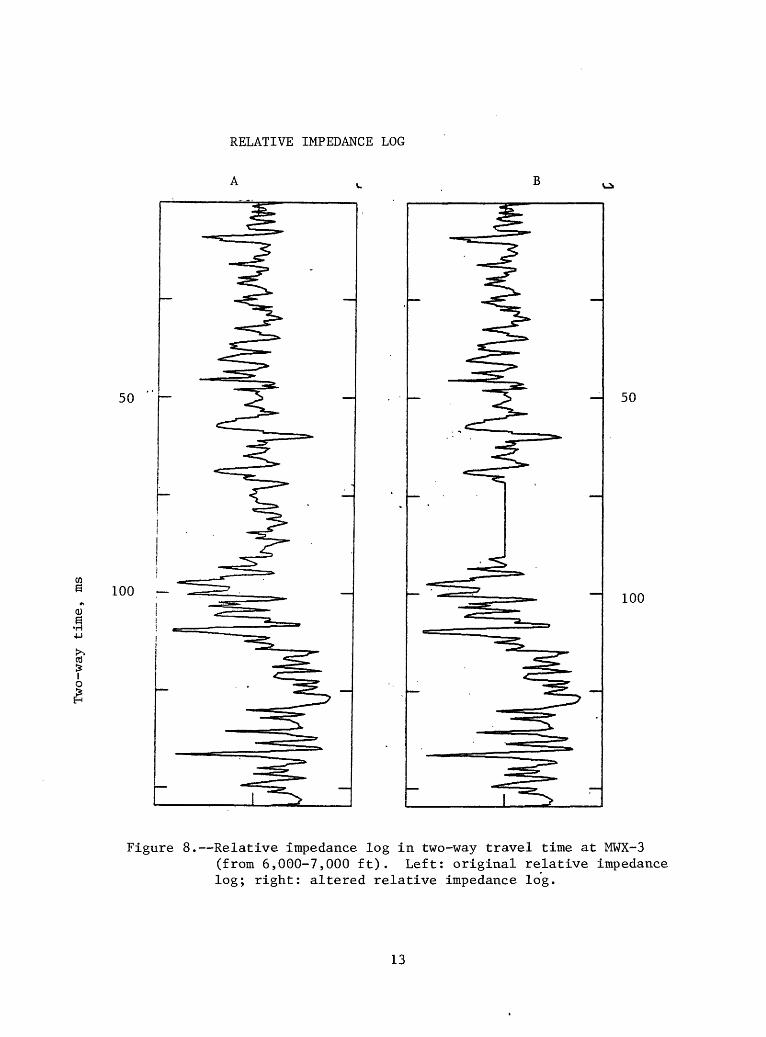
Figure 8 shows the impedance log in two-way travel time, derived from the sonic and density log at MWX-3 from a depth interval of 6,000 to 7,000 ft. Using this impedance log, synthetic seismograms were generated using various zero-phase bandpass filters as shown in figure 9.

The bottom part of figure 9 shows the seismic responses using 2/4 - 250/300 Hz wavelet. The top of the Yellow A sand body appears as a strong peak, the top of the Red A as a small peak, and the bottom of Red B as a small trough. By lowering frequency content, the character of the seismic response changes dramatically. The second panel from the bottom of figure 9 represents the seismic response using 2/4 - 72/100 Hz wavelet. Most of the seismic energy observed in the high-frequency section disappeared and overall amplitudes are much less than those of the high frequency version. So the same response was replotted using different gain in the third panel from the bottom. The top of figure 9 shows the response using 4/8 - 52/62 Hz wavelet, which is very similar to the observed frequency band.

As the frequency content gets lower, the base of the Red B appears as the strongest trough in the seismogram, and the peak representing the top of Yellow A in the high-frequency version is shifted to the later time. The overall seismic response in the frequency range of 4/8 - 52/62 Hz represents only the complicated interference peak and trough, and the whole of the lower coastal sand bodies appear within 3/4 of the dominant period.

The rather obvious question is, how much does the presence of the sand bodies in the lower coastal interval contribute to the overall seismic character shown in the top of figure 9? To answer this question, the lower portion of the near-offset VSP data (SL-1) was reprocessed very carefully. To minimize the spatial mixing of the upgoing waves during the multichannel velocity filtering, the inversion approach to extract upgoing waves (Lee, 1985) was implemented using two depth levels. Therefore, the maximum spatial uncertainty of the processed upgoing waves is in the range of one spatial sampling interval, which is 25 ft.

Figure 10 shows the downgoing wave with its amplitude spectrum at the well-phone depth of 6,000 ft, and upgoing wave field shifted to align the coherent events from 7,000 ft to 5,925 ft using the inversion method. The peak-trough combination shown in the top of figure 9 appears in the processed VSP data. The overall seismic character near the coastal sand bodies is very similar to the one derived from the impedance log.

In the VSP section, the trough corresponding to the base of Red B timewise appears to start from about 6,550 ft, which corresponds to the base of Red B depthwise. The preceding peak appears to start from about 6,425 ft, which corresponds to the top of Yellow A in depth. The sharpness of the downgoing wave at 6,000 ft (the top portion of figure 10) suggests that the preceding peak is not likely the result of the side lobe of the strong trough.

Based on the above analyses and observations, I concluded that the peak amplitude within the lower coastal interval was caused by the presence of the Yellow A, and the following trough represents the base of the Red B sand body.

12

RELATIVE IMPEDANCE LOG

50

100

50

100

Figure 8. Relative impedance log in two-way travel time at MWX-3(from 6,000-7,000 ft). Left: original relative impedance log; right: altered relative impedance log.

13

10 ms

Top of Yellow A 4^Bottom of Red B

of Red A

4/8-52/62 (Hz)

2/4-72/100 (Hz)

2/4-72/100 (Hz)

1^2/4-250/300 (Hz)

Figure 9. Synthetic seismogram generated from impedance log shown in fig Top: low-frequency version; bottom: high-frequency version.

14

CDP 2 DEPTH ORTfl TRRCE

6000

-I .Q_Q

40.03 50.00 60.00 TIMECMILS)

73.00 #10' 80.00 90.00

DECIBEL SPECTRUM

0.00 25.00 50.00 75.00FREQUENCY(HZ)

100.00 125.30

Figure 10. Identification of lower coastal zone at MWX-3 from SL-1. Top: downgoing wave and its amplitude spectrum at the wellphone depth of 6,000 ft; bottom: vertically aligned upgoing waves.

15

I was unable to estimate the contributions of the individual sand bodies in the Yellow zone (Yellow A, B, and C by Lorenz, 1984) and in the Red zone (Red A and B) to the overall seismic response. Therefore, I interpreted that the presence of the peak in the lower coastal interval represents the average seismic response from all of the Yellow sand bodies and the trough from all of the Red sand bodies. This peak-trough combination appears repeatedly throughout this study.

In order to examine and identify the seismic character of the lower coastal interval for other source locations, figures 11 and 12 were generated. In these figures, downgoing and upgoing waves from the depth range of 6,000-6,250 ft were vertically summed in order to improve signal-to-noise ratio, and various bandpass filters were applied. The same peak-trough combination appears for all the source locations with the correct time. The amplitude variations observed in figures 11 and 12 possibly are caused by the characteristics of spatial distribution of the lower coastal sand bodies and will be discussed further in the next section.

The peak-trough combination observed in the coastal interval for all source locations (figs. 11, 12) is the result of the presence of the sand bodies as proven by analysis of the well logs (Lorenz, 198U). However, it would be very interesting and helpful to analyze other possible acoustic impedance distributions which might result in similar peak-trough combinations further away from the well. This analysis is shown in figure 13. The lower part of the figure represents the seismic response with varying impedance of the lower coastal zone with 2/U - 250/300 Hz bandpass wavelet; the top part with U/8 - 52/62 Hz wavelet.

Model #1 represents the seismic response derived from the original impedance log, shown in the left part of figure 8. Model #2 represents the synthetic seismogram by replacing the lower coastal impedance by a constant relative impedance of 8, shown in the right part of figure 8, which corresponds to the average relative impedance of shale within the lower coastal zone. Model #3 represents the results by replacing the lower coastal interval by a constant relative impedance of 7. Model #U represents the seismic response by replacing the lower coastal interval by a constant relative impedance of 9, which corresponds to the average lower coastal sand impedance. Model #5 represents the seismic response replacing the lower coastal interval by a constant relative impedance of 6 which corresponds to the shale impedance below the coastal interval.

Some interesting observations can be made from figure 13. Models #3 and #5 cannot be fit into the observed seismic character because of the timing and amplitude mismatches. The remaining models #1, #2, and #U fit the observed data rather well. Models #1 and #M present no problem in interpreting the spatial distribution of the sand bodies, because these models represent sand bodies. However, model #2 creates some difficulties in interpreting the sand bodies further away from the well. If we assume that a sand body near the wellsite pinches out progressively away from the well into shale, it is very difficult to detect the truncation of the sand body, even though the amplitude response of the shale is slightly less than that of the sand.

Although different spatial distribution of sands and shales could provide some indication of the sand distribution, it may be quite difficult to analyze this amplitude variation using real VSP data. Thus, the possibility of the phase change into shale could be retained in the interpretation of the sand bodies.

16

DOWNGOING WAVE UPGOING WAVE

BASE OF COASTAL ZONE

SL-1

SL-2

Figure 11. Vertically summed, vertical-component data near top of the coastal zone at MWX-3 for SL-1 (top) and SL-2 (bottom) with various bandpass filters (upgoing wave amplified 4 times). A: 16/20-68/80 Hz; B: 12/16-68/80 Hz; C: 8/12-68/80 Hz; D: 4/8-68/80 Hz.

17

DOWNGOING WAVE UPGOING WAVE

D


SL-3

iSL-4

Figure 12. Vertically summed, vertical-component data near top of thecoastal zone and MWX-3 for SL-3 (top) and SL-4 (bottom) with various bandpass filters (upgoing wave amplified 4 times). A: 16/20-68/80 Hz; B: 12/16-68/80 Hz; C: 8/12-68/80 Hz; D: 4/8-68/80 Hz.

18

Top of Yellow A

10 ms

^ Bottom of Red B

Top of Red A

Figure 13. Synthetic seismograms replacing the impedance of lower coastalzone by various impedances. Top: low-frequency range (4/8-52/62 Hz); bottom: high-frequency range (2/6-250-300 Hz). 1: original; 2: relative impedance of 8; 3: relative impedance of 7; 4: relative impedance of 9; 5: relative impedance of 6.

19

Three-Dimensional Modeling

In order to determine the configuration of a finite body using an azimuthal VSP survey, one must investigate the seismic expression of the finitely extended body with respect to the VSP shooting geometry. A detailed three-dimensional modeling approach to this problem was reported by Lee (1984b). A brief discussion of the three-dimensional modeling pertinent to the interpretation of the lower coastal sand bodies follows.

Figure 14 shows the schematic diagram for the azimuthal VSP survey; the top part represents the plan view of the rectangular-type body with 3 different source locations; the bottom part represents the cross-sectional view from source location A. Source location A is located 3,000 ft along the axis of the body; location B is 3,000 ft perpendicular to the axis of the body; and location C is 300 ft along the axis of the body. This field configuration is very similar to the one adopted in the actual azimuthal survey conducted in this study.

Throughout the modeling experiment, the following parameters were used. The top of the body is 6,435 ft with a reflection coefficient of 0.1; the bottom of the body is 6,560 ft with a reflection coefficient of -0.2; the velocity is 13,000 ft/s; and 30 Hz Ricker wavelet was used.

In the bottom part of figure 14, the specular reflection point coming from the edge of the model is shown, and the distance from the target where the ray intersects with a borehole is denoted by Z . The amplitude response"

below Z consists of regular reflections from inside the body and the"

diffraction response from the edges of the body. However, the amplitude

response above Z consists of the diffraction only. The amplitude variation

near Z is the key factor to be considered in an attempt to map the edge. The

general behaviour of the amplitude variation near Z has been extensively

studied by Lee (1984a).

For all of the model responses shown in this report, seismic events appearing at 50 ms are reference amplitudes with a reflection coefficient of 0.1. The seismic response is plotted as a function of lateral distances from the borehole instead of the conventional depth. In this way, the seismic response can be compared to the laterally stacked VSP data more conveniently. The arrival time shown in the laterally stacked VSP data is the two-way travel time from the source to the reflecting horizon, while the arrival time shown in the model study is the time from the source to the reflector to the geophone location.

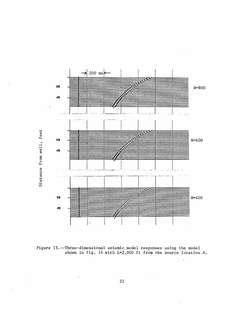
Figure 15 shows the seismic response of the rectangular body with L=2,000 ft and X =Y =0 with respect to the width of the body. In this geometry, all

of the specular reflection points are within the body. The dominant wavelength for this model is 433 ft; therefore, the width of the body is about 1, 1.5 and 2 of the source wavelength. The amplitudes at the lateral distance of 5 ft, or close to the well, are very close to each other, irrespective of the width of the body. But the amplitude at a greater lateral distances is quite different.

20

Y

Center of body (X ,Y ]

1 jj

A\

k L

c

'

? >

i

le-

Figure 1^* Plan (top) and cross-sectional view (bottom) of VSPconfiguration. L=length; W=width;(X ,Y )=the coordinate» o o7of the center of the body. A, B, and C represent source location.

21

I v-i

14-1

0)o

P CO

HP

95

45

95

45

95

45

200 ms

W=800

W=600

W=400

Figure 15. Three-dimensional seismic model responses using the modelshown in fig. 14 with L=2,000 ft from the source location A.

22

The amplitude at a lateral distance of 100 ft is about 1/4 that at the lateral distance of 5 ft for the 400-width body, and the amplitude decays rapidly as the lateral distance increases. For the 600-width body, the amplitude at 100 ft is about 3/4 that at a distance of 5 ft; there is not much amplitude difference with the lateral distance for the 800-ft body. The above observations would imply that if the width of the lenticular-type sand body is greater than 2 source wavelengths, the width of the body could be very insensitive to the seismic amplitude variation with respect to the lateral distance. If the width of the body is less than one source wavelength, the amplitude could decay rapidly with respect to the lateral distance.

Figure 16 shows the seismic response of the model shown in figure 15 except that the length of the body is altered to be infinite. Obviously, the seismic responses are very similar to each other except for a slight amplitude reduction in figure 16. This amplitude reduction is caused by the lack of constructive interference from the edges of the body.

Based on the results of figures 15 and 16, I conclude that near-offset VSP data can be used to interpret width, but not length, of the sand bodies. Figure 17 shows the seismic response of the rectangular-type body with L=2,000ft, W=600 ft, and X =Y =0 from the source locations A and B. The edge ' oo

amplitude, the amplitude at IQ in depth or Xg in lateral distance are shown in

figure 14, from source location A, is about 1/4 that at the lateral distance of 20 ft; while at source location B, about 1/2.

Figure 18 shows the seismic response of the same body with L=4,000 ft. The response from source location B is very similar to that shown in figure 17. This analysis implies that the length of the body might not be derived successfully by analyzing the VSP data with a source location in the perpendicular direction of the axis of the body.

Figure 19 shows the seismic response of the body modeled in figure 17 with a shift of the body 600 ft to the left, that is XQ = -600 ft. Comparing

figures 17, 18, and 19 reveals that the seismic response from source location B is very insensitive to the geometry of the body, but the amplitude decay with respect to the lateral distance is especially noticeable for the data from source location A. Therefore, the length of the truncated body can be estimated by analyzing the amplitude variations from the source location A.

The major amplitude-controlling factors not included in the three- dimensional model study are: (1) source radiation pattern, (2) angular dependence of the reflection coefficient, (3) attenuation, and (4) source and geophone coupling. Among the four major factors, some of the analyses for the first 3 factors can be done theoretically using a simplified homogeneous Earth model.

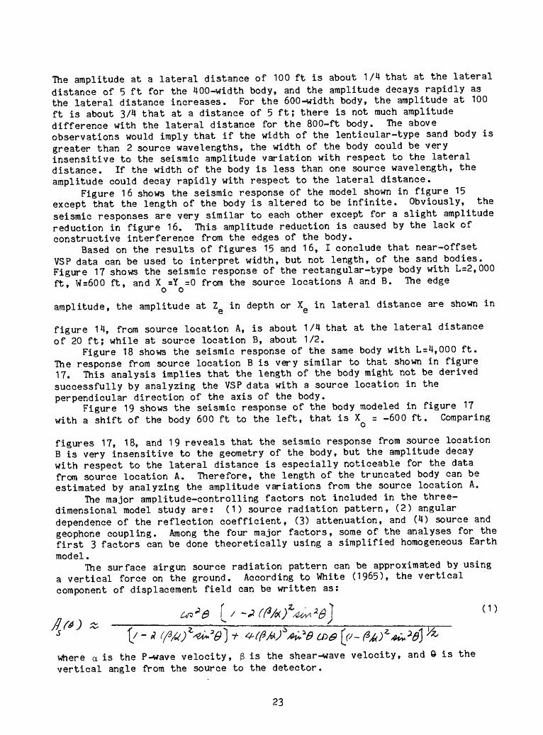
The surface airgun source radiation pattern can be approximated by using a vertical force on the ground. According to White (1965), the vertical component of displacement field can be written as:

c**eH f& ) ^s ~ {/ - A (f&f^B} i- ^(pMfti^e a><9 (V-

where a is the P^wave velocity, 3 is the shear-wave velocity, and » is the vertical angle from the source to the detector.

23

H-

OQ

C

i-j

(D

Distance fr

om well, feet

ho

-P-

en

H&

&

o

i-jS!

ft)

0

(D IH.

ex.

0

H- g

l-h

fD

H-

0

OQ

CO

H

- O

H-

0

H-

COn-

CD

&

H-

en^

9II

H-

H-

O

0 i-h

0

H-

O0

ex.H

- fD

n- ^

fDI-j

l-h

fD

i-j

CO

O

T3B

§n-

en

0*

fDfD

en

en

e

o

enC

H

- H

0

O

OQ

fDn-

M

P*

O

fD

O &3

3n-

o

H.

ex

.O

fD

0 M

ho o

o ^T

f -P> o

o

f ON

O

O

f oo o

o

1220

SL-A

SL-B

"-sms"f."^,sitr=i,:'2 ?v°siTop: from source location A; bottom: from source location B.

25

4-1enQ

1228

1323

923

626

428

228

28

1228

1828

823

628

428

228

200 ms

SL-A

;SL-B

1 Edge

Figure 18. Three-dimensional seismic model responses using the modelshown in fig. 14 with L=4,000 ft, W=600 ft, and X =Y =0.0.

o oTop: from source location A; bottom: from source location B

26

H-

OP

C

Dis

tance

fr

om w

ell

, fe

et

CO o c 0 fD H-1

O O fU rt H-

O 0 00

fU 0 (-^

oII o o H O ""O Mv

1-1 o 3 CO o C o fD h-1

O 0 PJ rt H-

O 0 Ji>

» cr

1o rt rt ?. M

iI-J O 3

I ICO

H

t?

0"*

0

i-i2

fD

0

fD 1H

« fi.

0

H.

3M

v fD

H-

0O

Q

CO

H*

0

Ul

03 H-1

H-

COrt

fD

0"

H-

COr<

3II

H-

K>

OX

o 3

0 0

O

DJ fD

Mv

h-1

rt v '"I fD

S3

COII

T3

^

O0

0

O

CO ft)M

vrt

C

< CO H

-X

0

O

OQ

II <T

i rt

O

E

rO

fD

Mv

3rt

O

OQ

fD

O o I

I bd

C/5f

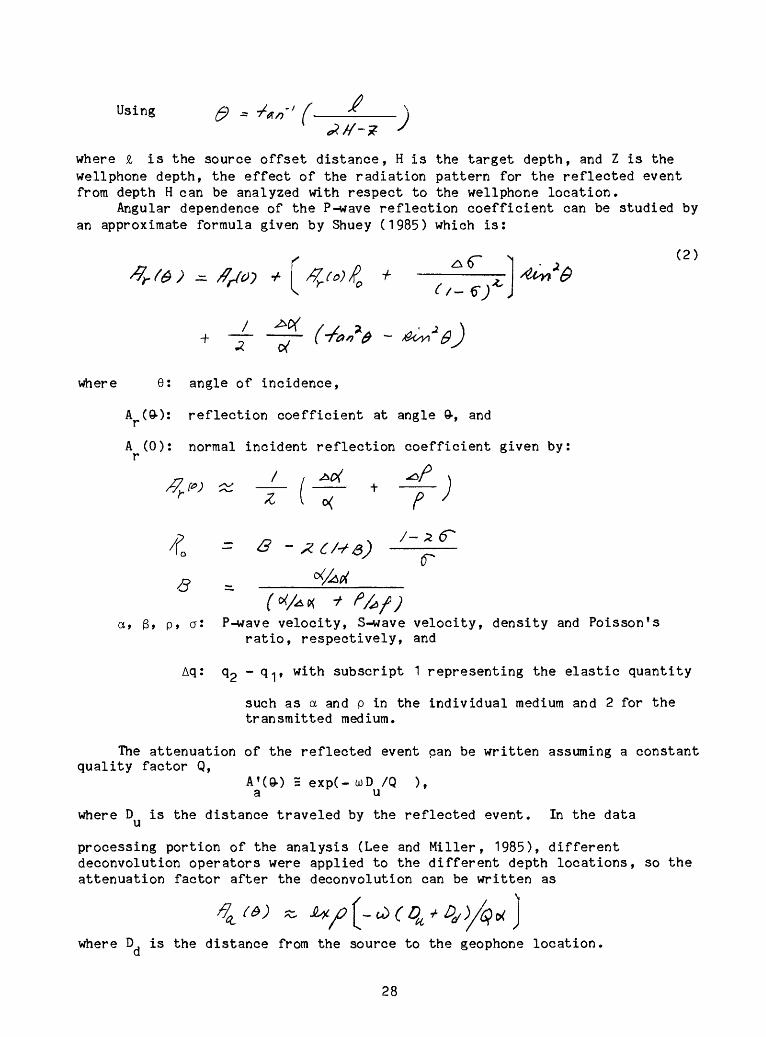
/Using

where £ is the source offset distance, H is the target depth, and Z is the wellphone depth, the effect of the radiation pattern for the reflected event from depth H can be analyzed with respect to the wellphone location.

Angular dependence of the P-wave reflection coefficient can be studied by an approximate formula given by Shuey (1985) which is:

t /

1 A rfwhere 6: angle of incidence,

A (90: reflection coefficient at angle 9-, and

A (0): normal incident reflection coefficient given by r

- G -

8 =,

^ I o< P

/-*6*

a, 3, p, a: P-wave velocity, S-wave velocity, density and Poisson's ratio, respectively, and

Aq: <\2 ~ QV with subscript 1 representing the elastic quantity

such as a and p in the individual medium and 2 for the transmitted medium.

The attenuation of the reflected event can be written assuming a constant quality factor Q,

A'(ft) = exp(- wD /Q ), a u

where D is the distance traveled by the reflected event. In the data

processing portion of the analysis (Lee and Miller, 1985), different deconvolution operators were applied to the different depth locations, so the attenuation factor after the deconvolution can be written as

where D is the distance from the source to the geophone location

28

In order to examine the three effects mentioned above, the following parameters were chosen for the computation:

£ = 3,000 ft

H = 6,500 ft

^ = 0.3, a 2 = 0.1

Q = 100

a 1 = 12,000 ft/s, c* 2 = 10,000 ft/s

P 1 = 2.5 g /cm3 , P 2 = 2.45 g /cm3

$ 1 = 6,500 ft/s

f = 25 Hz

Taking the reflected amplitude at depth location 6,500 ft as the reference amplitude, the amplitude variation due to the above-mentioned three effects can be written as:

4 &,) 4 where

9- = +**-

Figure 20 shows the computed amplitude variation with respect to the geophone location. The effect of the source radiation pattern is that the amplitude of the reflected vertical component is increasing with the decreasing well phone depth, and the reflection coefficient effect due to the angle of incidence is the opposite effect of the source radiation pattern. The attenuation effect is the most significant amplitude decaying factor with respect to the wellphone location.

In order to compensate for the amplitude decay of the seismic event

2 during the processing, a gain function T (where T is the arrival time) isapplied to the data. Therefore, the actual amplitude variation in the modeled data under this ideal and simplified condition, can be written as A times the gain function, which is shown in the figure as "amplitude after gain." As indicated in figure 20, the maximum amplitude reduction is about 13 percent, which cannot be a significant factor in the analysis of the sand body in the coastal zone. This conclusion could be applied to the real data analysis.

29

UJ o

2,0

00

4,0

00

ex 0)

Q

6,0

00

Reflection

coefficient

V

Amplitude after

gain

, Source radiation pattern

y. ^

,.;:

: ,...

Attenuation

XS.

XX

^ --4.

::

>^

Amplitude ratio

Gain function

X**

12.5

Figure 20. Reflection amplitude variation with respect to th

e source radiation pattern, angular

dependence reflection coefficient an

d attenuation.

Applied gain function T^

(T=time)

and

the

reflection amplitude after gain application are

also

shown.

Interpretation of Coastal Sand Bodies

The spatial distribution of the lower coastal sand bodies was interpreted using laterally stacked VSP data incorporating the geologic information by Lorenz (1985), well logs, one- and three-dimensional seismic modeling and other available VSP data. The laterally stacked VSP data used for the interpretation is shown in figures 21 to 25. The interpretation procedure is the following:

(1) Identify the peak-trough combination for the lower coastal interval.(2) Examine the continuity and character of the peak-trough combination

for the laterally stacked data in conjunction with other available VSP data.(3) Interpret the geometry of the Yellow and Red sand bodies using

amplitude variation near the edge incorporating the geologic information.(4) Perform the three-dimensional modeling based on interpretation of

step 3, and compare the model results with the real data for all four source locations.

(5) Adjust some of the model parameters to fit the real data.

The peak-trough combination, which represents the seismic response of the lower coastal interval, was identified for all source locations using vertically summed traces (figs. 11 and 12). Confirmation of the same peak-trough combination in laterally stacked data should increase the reliability of the data processing as well as interpretation. Figure 26 was produced by replacing the laterally stacked VSP data around 800 ft from source location #2, by the cumulative-summed traces from source location #1. This procedure is very similar to the conventional way of inserting the VSP data into the surface seismic data in order to carry out an accurate stratigraphic interpretation (Balch and others, 1982). The remarkable match of the key stratigraphic horizons between the two data sets should rule out any possible ambiguity in identifying the lower coastal interval, and the gross error in the processing should be small.

The initial interpretation of the lower coastal sand bodies (steps 1 through 3 of the interpretative procedure) follows.

The northwest edge of the base of the Red sand zone was interpreted primarily by the interference pattern and amplitude reduction around 400 ft from the well shown in figure 23, which is the laterally stacked SH-wave. A similar seismic character can be observed in the vertical-component data shown in figure 22. The northeast and southeast edges of the Red sand were interpreted using figures 24 and 25 by the amplitude reduction of the base of coastal reflection around 600 ft from the well. The length of the sand bodies cannot be estimated directly by this set of data, because there was no offset VSP to the southwest. Therefore, the length was estimated by step 5 of the interpretation procedure.

The interpretation of the Yellow zone was more complicated possibly due to the low reflection amplitude compared to the reflection from the base of the Red sand, and interferences with the upper coastal sand bodies. By the continuity of the peak reflection in figure 22, it was interpreted that the northwest edge of the Yellow sand could be beyond the maximum lateral distance investigated by the azimuthal survey, that is, about 1,200 ft from the well. The southeast edge of the Yellow was interpreted as an amplitude reduction around 250 ft from the well using figure 24.

31

Distance from well, feet

Distance from well, fe

et

OJ

H-

QTQ c H fD

K)

00

Ui

I OJ

l-h

Q

CO

CO

Of f

^I

fDI-

1 d.

O -d

o

H-

rt O

rt

rt

O S H-

rt

w CO w o

o CO H N

O W

o 4-1 d cd CO

H

P

1200

1000

600

600

400

200 Figure 22. Laterally

polarity;


stac

ked

and

cumu

lati

ve-s

umme

d ve

rtic

al-c

ompo

nent

da

ta at MWX-3

for

SL-2

. Le

ft:

normal

righ

t: reverse

polarity.

DISTANCE FROM WELL, FT

"'"*______ r^\mmmiimnm

^Jl tjj I >>i m jmjmSm mimiim^^^^^^^^^ss^^^Koirccccc

Figure 23. Laterally stacked and cumulative-summed SB-component data at MWX-3 from SL-2.

34

1000

Base of

coastal

zone

Figure 24. Laterally stacked

and

cumu

lati

ve-s

umme

d ve

rtic

al-c

ompo

nent

da

ta at MWX-3

from SL

-3.

Left

: normal polarity;

right: reverse

polarity.

0) cu M-l S o

}-i M-l CU

O J-J w

1201

3

10

00

800

600

400

200


Figu

re 25. Laterally stacked

and

cumulative-summed

vert

ical

-com

pone

nt da

ta at MW

X-3

for

SL-4

Le

ft:

reve

rse

polarity;

righ

t: normal po

lari

ty.

Time, secondsFigure 26. Laterally stacked vertical-component data at MWX-3 for SL-2 with subst^L-

tution at the laterally stacked data around 800 ft with the cumulative summed data for SL-1.

37

By performing interpretative steps 4 and 5 and taking into consideration the above observations, I made one possible interpretation of the lower coastal sand bodies as shown at the top of figure 27; the results of the three-dimensional modeling are shown in figures 27 to 30. This interpretation of the lower coastal sand bodies is similar to the interpretation based on the sedimentology of these zones by Lor en z (1985).

The amplitude variation of the near-offset data shown in figure 27 is similar to the real data shown in figure 21, which implies that the estimates for the average widths of the Yellow and Red sands are reasonable. The comparison between real and synthetic data for source location #2 reveals that the amplitude character of the trough reflections are similar. Notice the low amplitude and broadening of the trough reflection near the lateral distance of 600 ft both in synthetic and real data. For source location #3, the three-dimensional model does not indicate any amplitude reduction near 600 ft of the lateral distance. The reduction of the trough amplitude for source location #4 can be observed around 600 ft from the well.

Furthermore, numerous discrepancies exist between the real and synthetic data. The synthetic model may be too simple to explain the observed data, while the observed data were contaminated by noise.

As mentioned previously, the detection of the transition from sand to shale in the lower coastal interval in the one-dimensional case is very difficult to distinguish due to the similar seismic responses from sand and shale in one-dimensional cases. The effect of the transition in the three-dimensional case was examined by a model shown in the top of figure 31. The result of the modeling is shown in the bottom half of figure 31.

The difficulty of detecting the edge of the sand body which truncates into shale (based on the seismic response alone) is evident when the model result shown at the top of figure 18 (which modeled only the sand body) is compared to the model result shown in the bottom half of figure 31. One possible interpretation of the strong amplitude in the lower coastal interval beyond the interpreted edge of the sand from source location #4 may be established by the model shown in figure 31, but there is no other independent evidence to support this interpretation.

CONCLUSIONS

The detection of the edges of the lower coastal sand bodies using an azimuthal VSP survey proved to be difficult for the following reasons.

(1) The quality of the VSP data acquired under adverse field conditions was substantially degraded.

(2) The high-frequency required to map individual sand bodies could not be attained even by state-of-the-art technology due to the lack of impedance contrast between the sand and intervening shale and because of the small size of the sand body.

Even though some uncertainty in the interpretation remains, the following conclusions can be derived from the azimuthal VSP data at the MWX-3 well.

(1) The lower sand bodies (Yellow and Red) were identified with a high-level of confidence for all of the source locations.

(2) The Yellow sand bodies could extend more than 1,200 ft to the northwest of the well with average widths of 600 ft. The truncation edge could be to the southeast at about 400 ft.

38

3

J<».

1,000 ft

Sa 32O

OJ O£ttJ4J CO

rlO

Figure 27. Interpretation of lower coastal sand bodies (top) and3-dimensional model response (bottom) for SL-1 using 35 Hz Ricker wavelet.

39

910

710

sI SIB

318

lie

200

Figure 28. Three-dimensional model response for SL-2 using 25 Hz Ricker wavelet.

40

200 ms

0)o;

M-l

919

718

sia

313

lie


41

rH0)

1218

1818

818

618

0)oa 4i8cd

H P

218

18

200 ms


42

Plan view

Sand

1,000 ft

wellShale

source

Cross Section

r=0.1

Sand

r=0.2

r=0.08

Shale

r=-0.16

~~"6,435 ft

- 6,560 ft

iai8

S10

OJaa cd4-1 W H Q

210

200 ms

Shaletf-- I

Sand

Figure 31. Model simulating the transition from sand to shale (top) and this three-dimensional model response (bottom).

43

(3) The Red sand bodies could be oriented to the northeast with average widths of 800 ft and may be truncated at about 500 ft in the direction of source location 3. The position of the other edge could not be estimated directly from the VSP data because there was no source location opposite to source location 3; however, based on the three-dimensional model study, it could be extended more than 2,000 ft to the southwest.

(4) The extent of the upper coastal sand bodies could not be resolved due to their low and discontinuous amplitude responses, implying that the upper sand bodies may be smaller or thinner than the lower sand bodies.

(5) The general orientation of the Yellow and Red sand bodies based on the azimuthal VSP survey is similar to the interpretation based on the sedimentology of these zones by Lorenz (1985).

(6) An azimuthal VSP technique could be applicable for the delineation of the reservoir boundary if adequate field procedures are maintained.

REFERENCES CITED

Balch, A. H., Lee, M. W., Miller, J. J., and Ryder, R. T., 1982, Use ofvertical seismic profiles in seismic investigations of the Earth:Geophysics, v. 47, p. 906-918.

Lee, M. W., 1984a, Delineation of lenticular-type sand bodies by the verticalesismic profiling method: U.S. Geological Survey Open-File Report84-265, 92 p.

Lee, M. W., 1984b, Vertical seismic profiles at the multi-well experimentsite, Gar field Ccounty, Colorado: U.S. Geological Survey Open-FileReport 84-168, 57 p.

Lee, M. W., 1985, Inversion method in separating upgoing and downgoing waves(in press).

Lee, M. W., and Miller, J. J., 1985, Acquisition and processing of azimuthalvertical seismic profiles at multi-well experiment site, Garfield County,Colorado (in press).

Lorenz, J. C., 1984, Coastal zone sedimentology: Written communication, SandiaNational Laboratories.

Lorenz, J. C., 1985, Refined interpretations for the coastal zone: Writtencommunication, Sandia National Laboratories.

Sear Is, C. A., Lee, M. W., Miller, J. J., Albright, J. N., Fried, Jonathan,and Applegate, J. K., 1983, A coordinated seismic study of the multi-wellexperiment site: Society of Petroleum Engineers of AIME, SPE/DOE 1983,Symposium on Low Permeability Gas Reservoirs, Paper no. 11613, 10 p.

Shuey, R. T., 1985, A simplification of the Zoeppritz equations: Geophysics,v. 50, no. 4, p. 609-614.

White, J. E., 1965, Seismic waves: Radiation, transmission, and attenuation:New York, McGraw-Hill, 302 p.

44

Documents

Interpretation of Azimuthal Vertical Seismic Profile ... · Interpretation of Azimuthal Vertical Seismic ... component of the VSP data, one- and three-dimensional seismic ... interpretation