The time-averaged magnetic field in numerical dynamos with non-uniform boundary heat flow

Geophys. J. Int. (2002) 151, 809–823

The time-averaged magnetic field in numerical dynamoswith non-uniform boundary heat flow

Peter Olson1 and U. R. Christensen2

1Department of Earth and Planetary Sciences, Johns Hopkins University, USA. E-mail: [email protected] fur Geophysik der Universitat Gottingen, Germany

Accepted 2002 June 28. Received 2002 June 26; in original form 2001 November 14

S U M M A R YThe time-averaged geomagnetic field on the core–mantle boundary is interpreted using numeri-cal models of fluid dynamos driven by non-uniform heat flow. Dynamo calculations are made atPrandtl number Pr = 1, magnetic Prandtl numbers Pm = 1–2, Ekman numbers E = 3×10−4 –3 × 10−5 and Rayleigh numbers 10–30 times the critical value for different patterns of heatflow on the outer boundary of a rotating, electrically conducting spherical shell. The resultsare averaged over several magnetic diffusion times to delineate the steady-state magnetic fieldand fluid motion. When the boundary heat flow is uniform the time-averaged flow approachesaxisymmetry and the magnetic field is mostly a geocentric axial dipole (GAD). The largestdeparture from GAD in this case is the octupole field component. When the amplitude of theboundary heat flow heterogeneity exceeds the average heat flow, the dynamos usually fail.Lesser amounts of boundary heterogeneity produce stable dynamos with time-averaged mag-netic fields that depend on the form of the boundary heterogeneity. Elevated heat flow in thenorthern hemisphere produces a time-averaged axial quadrupole magnetic field comparable tothe inferred paleomagnetic quadrupole. Azimuthally periodic boundary heat flow produces atime-averaged magnetic field component with the same azimuthal wavenumber, shifted in lon-gitude relative to the heat flow pattern. Anomalously high and anomalously low magnetic fluxdensity correlate with downwellings and upwellings, respectively, in the time-averaged fluidmotion. A dynamo with boundary heat flow derived from lower-mantle seismic tomographyproduces anomalous magnetic flux patches at high latitudes and westward fluid velocity in onehemisphere, generally consistent with the present-day structure of the geodynamo.

Key words: dynamo models, Earth core dynamics, geodynamo, geomagnetic field, paleo-magnetic field, thermal convection.

1 I N T R O D U C T I O N

One of the fundamental assumptions in paleomagnetism is that themain geomagnetic field approaches a specific reference state whenaveraged over sufficiently long times. The reference state most com-monly used for the paleomagnetic field is a geocentric axial dipole,or GAD. Long-term departures from the reference GAD are particu-larly significant for the geodynamo, because they indicate influenceson the core by the mantle. Here we use numerical dynamo models toinvestigate how heat flow heterogeneity on the core–mantle bound-ary influences the geodynamo and the time-averaged structure ofthe geomagnetic field.

Palaeomagnetic data from uniform polarity epochs (that is, awayfrom times of polarity reversal or excursions), indicate two primaryways in which the geomagnetic field deviates from the GAD config-uration in time average. First, there is evidence from palaeomagneticinclinations from 0 to 5 Ma for a time-averaged axial quadrupolefield component. Relative to the axial dipole, the amplitude of this

axial quadrupole is 0.04–0.05 (Merrill et al. 1996; Dormy et al.2000). A persistent axial quadrupole term in the palaeomagneticfield, even a small one, is significant for the core, as it indicatesthat the geodynamo is not wholly symmetric about the equator inits long-term average behaviour. Secondly, there is a growing bodyof evidence from palaeomagnetic directions and intensities for de-viations from axisymmetry in the 0–5 Ma palaeomagnetic field(Johnson & Constable 1995, 1997; Kelly & Gubbins 1997;Constable et al. 2000; Kono et al. 2000). Deviation from axisymme-try in the time-averaged palaeomagnetic field is also significant; itindicates that some effect breaks the rotational symmetry imposedon the geodynamo by the Earth’s spin.

Because the timescale for magnetic field generation by motionin the fluid outer core is relatively short, of the order of 104 yr(Moffatt 1978), whereas the structure of the solid mantle changeson timescales of order 108 yr (Schubert et al. 2001), the long-termdepartures from GAD are generally thought to indicate some controlof the geodynamo by lateral heterogeneity in the D′′ region of the

C© 2002 RAS 809

810 P. Olson and U. R. Christensen

lower mantle. There are several types of lateral heterogeneity in theD′′ region that might plausibly influence the geodynamo, includinganomalous topography at the core–mantle boundary, lateral hetero-geneity in lower-mantle electrical conductivity, and lateral variationsin heat flow at the core–mantle boundary. The effects of these on thegeodynamo are usually referred to as topographic, electromagneticand thermal coupling, respectively (Buffett 2000).

In this paper we investigate some consequences of thermal core–mantle coupling on the time-averaged structure of the geomagneticfield, using numerical dynamo models. We focus on one aspect ofthermal coupling, the relationship of the pattern and amplitude ofcore–mantle boundary heat flow variations to the pattern and am-plitude of the time-averaged departures from GAD in the geomag-netic field. We use high-resolution numerical dynamo models basedon the full Navier–Stokes, magnetic induction and heat equations,without any ad hoc parametrizations, in order to delineate the phys-ical relationships between the boundary heat flow variations, thetime-averaged fluid motions within the core and the time-averagedstructure of the dynamo.

2 C O R E – M A N T L E T H E R M A LC O U P L I N G

The subject of thermal core–mantle coupling has a long history(Hide 1970; Vogt 1975; Jones 1977; Gubbins & Richards 1986;Gubbins & Bloxham 1987; Bloxham & Gubbins 1987; Bloxham &Jackson 1990; Gubbins 1997; Bloxham 2000a,b). Although many ofthe critical details are not yet understood, there is general agreementon the following basic mechanism. Because velocities of flow inthe liquid outer core are far larger than in the solid mantle, thecore and the mantle respond very differently to the continuity ofheat flow and temperature at the core–mantle boundary. The lowermantle sees the outer core as a perfect fluid, and sees the core–mantleboundary as stress-free and isothermal. In contrast, the fluid outercore sees the mantle as solid and sees the core–mantle boundary asrigid with a prescribed heat flow. In this way, core–mantle thermalinteraction is analogous to the thermal interaction between the oceanand the oceanic lithosphere. The lithosphere is sensitive to the oceantemperature at the sea floor, whereas the deep ocean is sensitive toheat flow variations imposed on it by the thermal structure of thelithosphere. In thermal core–mantle coupling the outer core plays arole similar to the ocean and the D′′-layer at the base of the mantleplays a role similar to the lithosphere.

Considerations of heat transfer across the core–mantle boundarysuggest that convection in the fluid outer core is influenced by thetemperature structure of the lower mantle in two ways. First, theaverage thermal gradient at the base of the mantle governs the totalheat flow from the core to the mantle. This, in turn, governs thecooling rate of the whole core, the rate of inner-core solidification,and the power available from convection to drive the geodynamo(Loper 1978; Lister & Buffett 1995; Labrosse et al. 1997). Sec-ondly, convection in the core responds to lateral variations in lower-mantle thermal structure, particularly to variations in heat flow at thecore–mantle boundary. Thermal convection in the core is enhancedwhere the core–mantle boundary heat flow is high and tends to besuppressed where the core–mantle boundary heat flow is low. Inaddition, a separate circulation system is produced within the outercore on the scale of the boundary heterogeneity.

Since core convection is the major energy source for the geody-namo, any long-term distortion of the convection pattern by non-uniform core–mantle boundary heat flow should affect the structure

of the time-averaged geomagnetic field. Accordingly, there shouldexist some relationship between the pattern of lower-mantle hetero-geneity (as revealed by seismic tomography for example), the patternof the time-averaged flow in the outer core, and the time-averagedstructure of the geomagnetic field. Also, because the pattern of man-tle heterogeneity evolves slowly, the coupling with the geomagneticfield should persist for millions of years and should be evident inthe structure of the palaeomagnetic field.

The actual variations in heat flow on the core–mantle boundarycan be inferred only very crudely, by assuming a certain relation-ship between seismic velocity variations and temperature variationsin the lower mantle. The usual assumption is that lateral temper-ature variations in the lower mantle are anticorrelated with lateralvariations in seismic velocity (Yuen et al. 1993). According to thisassumption, those portions of the D′′-layer with anomalously highseismic velocity (particularly high shear wave velocity) are relativelycold, and there the thermal gradient and the core–mantle boundaryheat flow are relatively high. Conversely, where D′′-layer seismicvelocities are low the mantle is relatively hot, and there the ther-mal gradient and the core–mantle boundary heat flow are relativelylow. This is the called the tomographic model of non-uniform core–mantle boundary heat flow. It has many shortcomings. For example,it ignores contributions to the seismic heterogeneity in the D′′-layerfrom compositional variations, which could alter the relationshipbetween shear wave velocity and heat flow. In addition, it does notconstrain the amplitude of the non-uniform part of the core–mantleboundary heat flow. In spite of these shortcomings, tomographicheat flow has often been used as a thermal boundary conditionfor numerical models of core–mantle thermal coupling (Olson &Glatzmaier 1996; Glatzmaier et al. 1999; Gibbons & Gubbins2000).

3 P R E V I O U S N U M E R I C A L S T U D I E S O FC O R E – M A N T L E T H E R M A L C O U P L I N G

The early numerical studies of core–mantle thermal coupling wereaimed at finding the conditions necessary for locking the non-axisymmetric parts of the convection and magnetic field to theboundary heat flow heterogeneity pattern. Zhang & Gubbins (1992,1993, 1996) showed that the azimuthal drift rate of the convectionplanform in a rotating sphere is affected by thermal heterogene-ity on the boundary. For small-amplitude convection near the crit-ical Rayleigh number, where the planform is azimuthally periodic,Zhang & Gubbins (1996) found steady states in which the azimuthaldrift rate vanishes and the convection planform becomes stationarywith respect to the boundary heterogeneity.

Gibbons & Gubbins (2000) used numerical models of finite am-plitude rotating convection subject to spherical harmonic degreeand order two boundary heat flux variations to determine the lon-gitudinal phase relationship between the boundary heat flow andconvection at higher Rayleigh numbers. At low rotation rates (rel-atively large Ekman number), they found the radial motion to benegatively correlated with the boundary heat flow. Downwellingsoccur beneath the high boundary heat flow sectors, where the fluidtemperature is lowest. As the rotation rate is increased, they foundthe locked convection planform shifts progressively eastward, so thatat the highest rotation rates considered (corresponding to an Ekmannumber E = 10−4), the locked downwellings are located east of thehigh heat flow sectors, close to the longitude where the boundaryheat flow anomaly is zero.

At higher Rayleigh numbers, rotating convection becomeschaotic, in addition to being intrinsically time dependent. In this

C© 2002 RAS, GJI, 151, 809–823

Magnetic field in numerical dynamos 811

regime, thermal coupling occurs only in a statistical sense, as shownfor rotating convection by Sun et al. (1994) and for rotating mag-netoconvection by Olson & Glatzmaier (1996). The presence of amagnetic field and strong Lorentz forces further complicate the rela-tionship between the convection pattern and the boundary heating.For this reason, numerical dynamo models are preferable to bothrotating convection or rotating magnetoconvection for investigatingcore–mantle thermal coupling, because the dynamo models includethe Lorentz force in a dynamically consistent way. A drawback ofdynamo models is that they are more expensive to run, so fewercases can be examined.

Sarson et al. (1997) examined the relationship between magneticfield, fluid velocity and boundary heating patterns using a so-called2.5-dimensional numerical dynamo model, in which the azimuthalvariation is restricted to wavenumbers m = 0 and 2. They find thatthe fluid motion and the magnetic field near the outer boundary aresimply related: high magnetic flux density regions are located overthe fluid downwellings, and low magnetic flux density regions arelocated over fluid upwellings. However, Sarson et al. (1997) alsofound that the relationship between the boundary heat flow patternand the fluid motion is not so simple, and depends on the relativestrength of the Lorentz and Coriolis forces, that is, on the Elsassernumber �. For small �, rotation shifts the convection planform tothe east of the boundary heat flow pattern, whereas at larger � therelationship is reversed, and the convection planform is shifted tothe west of the boundary heat flow pattern.

The extreme truncation of azimuthal wavenumbers in2.5-dimensional dynamo models limits their application to situa-tions where the Rayleigh number of the convection is close to thecritical value. Dynamo models with fully developed (highly super-critical) convection and low Ekman numbers show that the convec-tion consists of narrow, quasi-geostrophic columns that are chaot-ically time dependent. In this regime it is unlikely that the entiredynamo would be locked to the boundary heat flow pattern. Instead,we expect that part of the magnetic field would be variable in time,so that the effects of the boundary heterogeneity would be seenbest in long-term averages. Coe et al. (2000) analysed the time-averaged structure of some time-dependent dynamos with polarityreversals calculated by Glatzmaier et al. (1999). For a boundary heatflow pattern derived from lower-mantle seismic tomography, the dy-namo model of Glatzmaier et al. (1999) shows a positive correlationbetween heat flow and the time-averaged non-dipole field: the non-dipole magnetic field on the outer boundary is most intense wherethe heat flow is highest (Coe et al. 2000). A qualitatively similarresult has also been reported by Bloxham (2001), using a differenttime-dependent numerical dynamo model. Two explanations havebeen given for the correlation between high heat flow and high mag-netic field intensity on the boundary. One is that the time-averaged(residual) fluid downwellings are located beneath high boundaryheat flow regions, and concentrate the magnetic flux there. Anotherexplanation is that the small-scale columnar convection is locallyintensified beneath high boundary heat flow regions, and the inten-sified convection induces an anomalously strong magnetic field. Ofcourse, it is possible that the two effects work together. The impor-tant point is that both of these mechanisms predict a close spatialrelationship between the non-uniform boundary heat flow and themagnetic field intensity.

Dynamo models have also been used to interpret axisymmetricdepartures from GAD. Recently, Bloxham (2000b) obtained a strongaxial octupole contribution to the time-averaged magnetic field byimposing a boundary heat flux pattern of spherical harmonic ordertwo and degree zero. He also found that a pattern of spherical har-

monic degree and order two had little effect on the axisymmetricpart of the magnetic field.

4 N U M E R I C A L M O D E L

We use a modified version of the numerical dynamo model devel-oped by G. A. Glatzmaier and described in Olson et al. (1999) andChristensen et al. (1999). We consider 3-D, time-dependent thermalconvection in an electrically conducting, incompressible Boussi-nessq fluid in a rotating spherical shell. The governing equationsare: (1) the Navier–Stokes equation with full inertia, Coriolis, andLorentz forces, using constant Newtonian viscosity; (2) the heattransport equation for the temperature; (3) the induction equationfor the magnetic field. The spherical shell has the same ratio of innerradius ri to outer radius ro as the Earth’s outer core, ri/ro = 0.35.Both spherical boundaries are assumed to be rigid, impermeable andelectrically insulating. The electrically insulating outer boundarycondition is a justifiable approximation for the core–mantle bound-ary, since the mantle is much less conducting than the core. Ourassumption of an electrically insulating inner boundary conditionis a matter of numerical convenience. It is not a priori justifiablefor the inner-core boundary, because the electrical conductivity ofthe solid inner core is expected to be comparable to the fluid outercore (Secco & Schloessin 1989). However, in a separate study usingthis model, Wicht (2002) finds only minor differences in the be-haviour of dynamos with electrically conducting versus insulatinginner-core boundaries. In particular, he finds very small differencesin the time-averaged fields with and without inner-core conduc-tivity. Since we consider dynamos in the same general parameterrange as Wicht, we are confident that our interpretations of the time-averaged states in this study apply equally to models with the sameparameters but with conducting inner cores. In this study we ex-amine numerical dynamos in the fully developed regime of Olsonet al. (1999). These dynamos are dominated by stable, non-reversing,nearly axial dipole magnetic fields, and produce well-defined time-averaged states. Magnetic reversals have been obtained with themodel we use here, but at significantly larger Rayleigh numbers,where the dipole field is more time variable (Kutzner & Christensen2002).

The thermal boundary conditions we use are as follows. The innerboundary is isothermal, with a prescribed uniform temperature. Theouter boundary has prescribed heat flow. The local heat flux on theouter boundary q is the sum of a surface average qo plus a spatiallyvariable part q ′(θ, φ) representing the boundary heterogeneity. Wedefine the heterogeneity amplitude q∗ as half the ratio of the peak-to-peak boundary heat flow heterogeneity to the average; that is,

q∗ = q ′max − q ′

min

2qo. (1)

The results of calculations using several different spatial patternsof the boundary heat flow heterogeneity are compared. These in-clude uniform heating (q∗ = 0), patterns consisting of individualspherical harmonics q ′ ∼ Y m

l , and a tomographic pattern derivedby assuming −q ′ has the same pattern as the first four sphericalharmonic degrees in the model of lower-mantle seismic shear waveheterogeneity by Masters et al. (1996). We refer to these differentcases as uniform Ylm and tomographic, respectively.

In addition to the boundary heterogeneity amplitude, the otherdimensionless input parameters are the Rayleigh number Ra, theEkman number E, the Prandtl number Pr and the magnetic Prandtlnumber Pm. The lower the Ekman number, the higher the spatial

C© 2002 RAS, GJI, 151, 809–823


Table 1. Dynamo model parameters.

Input parameter Definition Range

Prandtl number Pr = ν/κ 1Magnetic Prandtl Pm = ν/λ 1–2

numberEkman number E = ν/�D2 0.3–3 × 10−4

Rayleigh number Ra = αgoqo D4/kκν 2.5 × 106–2 × 108

Boundary heterogeneity q∗ = (q ′max − q ′

min)/2qo −0.5 to +1.25

Output parameter Definition Outer coreMagnetic Reynolds Re = u D/λ 500

numberElsasser number � = σ B2/ρ� ∼1Gauss ratios (Glm, Hlm) = (gm

l , hml )/g0

1 −0.1 to +0.1

Notes: D = ro − ri shell thickness; ν, κ, λ viscous, thermal, magneticdiffusivities; k thermal conductivity; σ electrical conductivity; α thermalexpansivity; go outer boundary gravity; ρ average density; � rotationangular velocity; qo, q ′ mean, variable boundary heat flows; u fluidvelocity; B magnetic induction; gm

l time-averaged magnetic field Gausscoefficients.

and temporal resolution that is required. In our calculations we trun-cate at spherical harmonic degree lmax = 53 at E = 3 × 10−4 andlmax = 106 at E = 3 × 10−5. These spherical harmonic truncationswere chosen on the basis of spectral resolution tests by Christensenet al. 1999 at E = 1 × 10−4. As shown in Fig. 10 (in Section 5), thetime-averaged magnetic field spectra decrease by at least a factor of103 over this spectral range. Our lowest Ekman number is severalorders of magnitude too large for the core, even if a turbulent vis-cosity is assumed, so the viscosity and thermal diffusivity are moreimportant in our calculations than in the core.

Two important output parameters are the volume-averagedElsasser number �, a measure of the dynamo magnetic fieldstrength, and the volume-averaged magnetic Reynolds number Rm,a measure of the fluid velocity in the dynamo. To characterize thedepartures of the time-averaged magnetic field from the referenceGAD, we follow the convention used in palaeomagnetism (Merrillet al. 1996), in which magnetic field anomalies are described us-ing ratios of individual Gauss coefficients gm

l or hml to the Gauss

coefficient of the axial dipole magnetic field g01 . We refer to these

as Gauss ratios, Glm or Hlm, respectively. The definitions of thedimensionless parameters in terms of physical quantities are givenin Table 1. Table 2 gives the notation of all the variables we usein analysing the calculations, the fundamental scaling for the basicvariables and the numerical values of the scalefactors we use forconverting our results to dimensional form.

The calculations are started from dynamo solutions that wereobtained previously using isothermal boundary conditions but oth-erwise with comparable parameters (Christensen et al. 1999). Whenthermal equilibrium is reached, as indicated by statistically steady

Table 2. Scaling.

Notation Variable Scale factor Value

θ, φ Colatitude, east longitude — —r Radius D 2260 kmt∗ Averaging time D2/λ 122 000 yrBr Radial magnetic field at ro

√ρ�/σ 1.16 mT

ur Radial velocity near ro λ/D 5.87×10−7 m s−1

ψ Toroidal streamfunction near ro λ 1.33 m2 s−1

To Temperature at ro Dqo/k —

flow, the outer boundary condition is changed from the prescribedtemperature to the prescribed heat flow. Each calculation is thencontinued beyond its initial transient response to the new bound-ary condition, until an approximate global equilibration is reached,where the time-series of total magnetic and kinetic appear to be sta-tistically stationary. We then continue the calculation and computerunning time averages of the temperature, velocity and magneticfields. These time averages provide the basic data for our analysis.We stop the calculation at an averaging time t∗ when the change inthe time-averaged radial magnetic field at the outer boundary Br be-comes sufficiently small. As used here, the term ‘sufficiently small’is somewhat arbitrary. We have adopted a practical definition, inwhich a calculation is stopped when the large-scale pattern of Br

on the outer boundary has stabilized. The averaging times shown inTable 2 are given in magnetic diffusion time units, based on the fluidshell thickness. In terms of our scaling, one magnetic diffusion timeis very nearly equal to four dipole diffusion times. Assuming anelectrical conductivity of σ = 6 × 105 S m−1 (Secco & Schloessin1989) for example, one magnetic diffusion time unit corresponds toapproximately 122 000 yr in the core.

Finally, we point out that all of the dynamo solutions shown inthis paper have magnetic fields dominated by a dipole componentwith ‘reversed’ polarity, that is, a polarity opposite to the present-day geomagnetic field. The reverse dipole polarity is a result ofthe initial conditions we use, and otherwise has no effect on ourinterpretations.

5 R E S U LT S

Table 3 gives the input parameters for all the calculations in termsof the notation from the previous section. Table 3 also summa-rizes some of the important results for each case, including theElsasser and magnetic Reynolds numbers, the time-averaged ki-netic and magnetic energies (as defined in Olson et al. 1999), andthe Gauss coefficient of the axial dipole part of the time-averagedmagnetic field, g1

0 .Most of the calculations we analyse are made at Ra = 2.5 × 106

and E = 3 × 10−4. As shown in Table 3, the magnetic energy ex-ceeds the kinetic energy in these cases, although not by as much as itprobably does in the core. Table 3 also shows the volume-averagedmagnetic Reynolds and Elsasser numbers are about 145 and 5, re-spectively, in these dynamos. These are broadly in the range of thegeodynamo, although they are slightly low and slightly high, respec-tively, compared with typical estimates from the present-day geo-magnetic field. Similarly, the Gauss coefficients of the axial dipoleg0

1 are typically 60 per cent higher than the present-day geomagneticfield. For comparison purposes we have also included two additionalcases of the Y22 boundary heating pattern at higher Rayleigh numberand lower Ekman number, respectively.

Fig. 1 shows the structure of the dynamo with uniform boundaryheating averaged over t∗ = 6.7 magnetic diffusion times, equivalentto about 800 000 yr in the core. The flow pattern in Figs 1(a) and (b)is taken close to the boundary but below the viscous Ekman layer.The time-averaged magnetic field and fluid motion are nearly ax-isymmetric and nearly antisymmetric about the equator. The smalldepartures from true axisymmetry seen in the figure are tending to-ward zero with increasing averaging time. The time-averaged mag-netic field in Fig. 1(c) is clearly dominated by the GAD component.The most noticeable departure from GAD is seen at high latitudesin both hemispheres, and consists of a low-intensity field directlyover the poles, the polar cap minima and rings of high-intensity

C© 2002 RAS, GJI, 151, 809–823


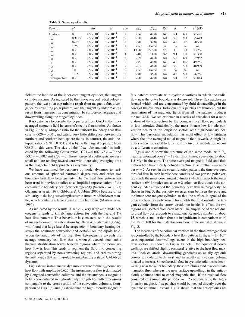
Table 3. Summary of results.

Pattern q∗ Ra E Pm Ekin Emag Rm � t∗ g01 (nT)

Uniform 0 2.5 × 106 3 × 10−4 2 2540 4280 143 5.1 6.7 57 620Y22 0.3125 2.5 × 106 3 × 10−4 2 2580 4140 144 5.0 9.3 55 643Y22 0.625 2.5 × 106 3 × 10−4 2 2700 3730 147 4.5 12 50 500Y22 1.25 2.5 × 106 3 × 10−4 2 Failed Failed na na na naY22 0.5 2.8 × 107 1 × 10−4 2 13 500 27 500 329 11 3.3 73 756Y22 0.5 2.0 × 108 3 × 10−5 1 35 400 15 100 266 9.1 1.0 81 300Y10 0.5 2.5 × 106 3 × 10−4 2 2590 4450 144 5.3 6.9 57 962Y11 0.5 2.5 × 106 3 × 10−4 2 2750 4030 148 4.8 8.6 49 765Y20 0.5 2.5 × 106 3 × 10−4 2 2630 4670 145 5.6 5.3 48 989Y20 1.0 2.5 × 106 3 × 10−4 2 Failed Failed na na na naY20 −0.5 2.5 × 106 3 × 10−4 2 2700 3560 147 4.3 5.3 56 766Tomographic 0.5 2.5 × 106 3 × 10−4 2 2600 4270 144 5.1 7.2 53 014

field at the latitude of the inner-core tangent cylinder, the tangentcylinder maxima. As indicated by the time-averaged radial velocitypattern, the two polar cap minima result from magnetic flux diver-gence by upwelling polar plumes, and the tangent cylinder maximaresult from magnetic flux concentration by surface convergence anddownwelling along the tangent cylinder.

It is customary to describe the departures from GAD in the time-averaged magnetic field in terms of specific Gauss ratios. As shownin Fig. 2, the quadrupole ratio for the uniform boundary heat flowcase is G20 = 0.001, indicating very little difference between thenorthern and southern hemisphere fields. In contrast, the axial oc-tupole ratio is G30 = 0.061, and is by far the largest departure fromGAD in this case. The size of the ‘flux lobe anomaly’ is indi-cated by the following Gauss ratios: G31 = 0.002, H31 = 0 andG32 = −0.002 and H32 = 0. These non-axial coefficients are verysmall and are tending toward zero with increasing averaging timeas the magnetic field approaches axisymmetry.

We have examined the response of model dynamos to vari-ous amounts of spherical harmonic degree two and order twoboundary heat flow heterogeneity. The Y22 heat flow pattern hasbeen used in previous studies as a simplified representation of thecore–mantle boundary heat flow heterogeneity (Sarson et al. 1997;Glatzmaier et al. 1999; Gibbons & Gubbins 2000) because of itssimilarity to the long-wavelength seismic structure of the lower man-tle, which contains a large signal at this harmonic (Masters et al.1996).

As indicated by the results in Table 3, very large amplitude het-erogeneity tends to kill dynamo action, for both the Y20 and Y22

heat flow patterns. This behaviour is consistent with the resultsof magnetoconvection calculations by Olson & Glatzmaier (1996),who found that large lateral heterogeneity in boundary heating de-stroys the columnar convection and destabilizes the dipole field.When the amplitude of the heat flow heterogeneity exceeds theaverage boundary heat flow, that is, when q∗ exceeds one, stablethermal stratification forms beneath regions where the boundaryheat flow is low. This tends to segment the fluid into convectingregions separated by non-convecting regions, and creates strongthermal winds that are ill-suited to maintaining a stable GAD-typedynamo.

Fig. 3 shows instantaneous dynamo structure for the Y22 boundaryheat flow with amplitude 0.625. The instantaneous flow is dominatedby elongated convection columns, and the instantaneous magneticfield is concentrated in high-intensity flux patches with dimensionscomparable to the cross-section of the convection columns. Com-parison of Figs 3(a) and (c) shows that the high-intensity magnetic

flux patches correlate with cyclonic vortices in which the radialflow near the outer boundary is downward. These flux patches areformed within and are concentrated by fluid downwellings in thecores of the cyclones. Individual flux patches are transient, but thesummation of the magnetic fields from all the patches producesthe net GAD. We see evidence in a series of snapshots for a mod-ulation of the convection by the boundary heat flow, particularlyat low latitudes. Statistically, the most intense low-latitude con-vection occurs in the longitude sectors with high boundary heatflow. This particular modulation has most effect at low latitudeswhere the time-averaged radial magnetic field is weak. At high lat-itudes where the radial field is most intense, the modulation occursby a different mechanism.

Figs 4 and 5 show the structure of the same model with Y22

heating, averaged over t∗ = 12 diffusion times, equivalent to about1.5 Myr in the core. The time-averaged magnetic field and fluidmotion both have clearly defined structure at azimuthal wavenum-ber m = 2. As seen in the streamfunction pattern, the time-averagedtoroidal flow in each hemisphere consists of two parts: a polar vor-tex inside the inner-core tangent cylinder (which intersects the outersurface at 69◦ latitude), and an m = 2 columnar flow outside the tan-gent cylinder attributed the boundary heat flow heterogeneity. Asshown in Fig. 5, the vorticity reverses sign between the pole andthe inner-core tangent cylinder, so that the surface integral of thepolar vortices is nearly zero. This shields the fluid outside the tan-gent cylinder from the vortex circulation inside; in effect, the tworegions are isolated from each other. The amplitude of the residualtoroidal flow corresponds to a magnetic Reynolds number of about15, which is smaller than (but not insignificant in comparison with)the Rm � 100 for the instantaneous flow in the snapshot shown inFig. 3.

The locations of the columnar vortices in the time-averaged floware controlled by the boundary heat flow pattern. In the E = 3×10−4

case, equatorial downwellings occur in the high boundary heatflow sectors, as shown in Fig. 4. In detail, the equatorial down-wellings are shifted slightly eastward relative to the heat flow max-ima. Each equatorial downwelling generates an axially cyclonicconvection column to its west and an axially anticyclonic columnlocated to its east. Since the axial flow in cyclonic columns is down-welling near the outer boundary, these structures tend to accumulatemagnetic flux, whereas the near-surface upwellings in the anticy-clonic columns tend to expel magnetic flux. If the residual flowconsisted of azimuthally periodic m = 2 columns only, the high-intensity magnetic flux patches would be located directly over thecyclonic columns. Instead, Fig. 4 shows that the anticyclones are

C© 2002 RAS, GJI, 151, 809–823


(a)

(c)

(b)

Figure 1. Time-averaged dynamo with uniform boundary heat flow. (a) Toroidal streamlines at depth ro − r = 0.04, contour interval 1; (b) radial velocity atdepth ro − r = 0.04, contour interval 0.8; (c) radial magnetic field at ro, contour interval 0.16. Dark = positive, light = negative.

slightly stronger than the cyclones, and in addition, there is also mag-netic flux concentration by the axisymmetric downwelling along thetangent cylinder. The effect of this combination of flows is to dis-place the magnetic flux patches poleward and eastward from thecyclone centres.

The specific relationship between the magnetic flux patches andthe residual circulation can be understood in terms of a balance be-tween magnetic field line stretching by downwellings and upwellingsversus magnetic diffusion. At high latitudes, the dominant compo-nent of magnetic diffusion is tangential, that is, diffusion over thespherical surface. The balance of these terms in the time-averaged

magnetic induction equation for the radial component of the mag-netic field near the outer boundary r0 gives

Br ur � (ro − r )∇2H Br , (2)

where Br and ur are time averages of the dimensionless radialmagnetic field and radial fluid velocity, respectively. Accordingto eq. (2), the anomalously low-intensity flux patches (for exam-ple, patches in the northern hemisphere where ∇2

H Br is large andpositive) are related to the fluid upwellings (ur > 0), and anoma-lously high-intensity flux patches are related to fluid downwellings

C© 2002 RAS, GJI, 151, 809–823


-0.01

0.00

0.01

0.02

0.03

0.04

0.05

0.06

0.07

H11

H11

G11

G11

G21

G21

G20

G20

G22

G22

H21

H21

G30

G30

H22

H22

H31

H31

G31

G31

H32

H32

G32

G32

-0.02

-0.01

0.00

0.01

0.02

0.03

0.04

0.05

0.06

H11

G11

G11

G21

G20

G22

H21

G30

H22

H31

G31

G31

H32

G32

G32

-0.01

0.00

0.01

0.02

0.03

0.04

0.05

0.06

0.07

0.08

H11

H11

G11

G11

G21

G21

G20

G20

G22

G22

H21

H21

G30

G30

H22

H22

H31

H31

G31

G31

H32

H32

G32

G32

-0.02

-0.01

0.00

0.01

0.02

0.03

0.04

0.05

0.06

H11

G11

G11

G21

G20

G22

H21

G30

H22

H31

G31

G31

H32

G32

G32

-0.02

-0.01

0.00

0.01

0.02

0.03

0.04

0.05

0.06

0.07

0.08

H11

G11

G21

G20

G22

G22

H21

G30

H22

H31

G31

H32

G32

G32

UniformY22

Y10

Y11

TOMOGRAPHIC

-0.01

0.00

0.01

0.02

0.03

0.04

-Y20

(a) (b)

(c) (d)

(e) (f)

H11

H11

G11

G11

G21

G21

G20

G20

G22

G22

H21

H21

G30

G30

H22

H22

H31

H31

G31

G31

H32

H32

G32

G32

Figure 2. Ratios of Gauss coefficients normalized by the GAD term g01 from the time-averaged magnetic fields of six cases with different boundary heat flow

patterns in Table 3. (a) Uniform; (b) Y22, q∗ = 0.625; (c) Y10, q∗ = 0.5; (d) Y20, q∗ = 0.5; (e) Y11, q∗ = 0.5; (f) tomographic, q∗ = 0.5. The error bars indicatethe range of palaeomagnetic estimates of the ratios G20 and G30.

(ur < 0). The relationship implied by (2) can be seen by comparingFigs 5(b) and (d), which shows the close similarity between ur and∇2

H Br over the northern hemisphere of the dynamo model.A linear relationship between the amplitude of the anomalous

magnetic field and the amplitude of the boundary heat flow hetero-

geneity can be seen from the results of calculations with the sameheat flow pattern but different amplitudes. Fig. 2 shows the Gaussratios G2

3 and H 23 used to characterize the magnetic flux patches

produced by the Y22 boundary heat flow variation with q∗ = 0.625.Comparing these ratios with the same ratios from the other Y22-type

C© 2002 RAS, GJI, 151, 809–823


(a)

(b)

(c)

Fig

ure

3.S

naps

hots

ofdy

nam

ow

ith

Y22

boun

dary

heat

flow

patt

ern,

q∗ =

0.62

5,E

=3

×10

−4.

(a)

Toro

idal

stre

amli

nes

atr o

−r=

0.04

,co

ntou

rin

terv

al3,

over

boun

dary

heat

flow

hete

roge

neit

y;(b

)ra

dial

velo

city

atde

pth

r o−

r=

0.04

,co

ntou

rin

terv

al4;

(c)

radi

alm

agne

tic

fiel

dat

r o,

cont

our

inte

rval

0.4.

Red

=po

sitiv

e,bl

ue=

nega

tive.

(a)

(b)

(c)

Fig

ure

4.T

ime-

aver

aged

dyna

mo

wit

hY

22bo

unda

ryhe

atfl

owpa

tter

n,q

∗ =0.

625,

E=

3×

10−4

.(a

)To

roid

alst

ream

line

s(w

ith

velo

city

dire

ctio

nar

row

s)at

dept

hr o

−r=

0.04

,co

ntou

rin

terv

al1.

0,ov

erbo

unda

ryhe

atfl

owhe

tero

gene

ity;

(b)

radi

alve

loci

tyat

dept

hr o

−r=

0.04

,con

tour

inte

rval

0.8;

(c)

radi

alm

agne

tic

fiel

dat

r o,c

onto

urin

terv

al0.

16.D

ark

=po

sitiv

e,li

ght=

nega

tive.

C© 2002 RAS, GJI, 151, 809–823


cases in Table 3 indicates that the amplitudes of G32 and H32 aredirectly proportional to the non-uniform heat flow amplitude q∗.

Most of our conclusions are drawn from cases with Ekman num-ber E = 3×10−4. This Ekman number allows for calculations witha long averaging time t∗ and provides well-defined time-averagedflow and magnetic field structures. For comparison, we have alsoexamined dynamos with the same Y22 boundary heat flow patternbut lower Ekman number, specifically E = 1 × 10−4 and 3 × 10−5.Some of the global properties of the time-averaged results of thesecases are given in Table 3. The cases with lower Ekman numberhave shorter averaging times. However, the same basic structuresin the time-averaged magnetic field seen in Figs 4 and 5 are alsopresent in the lower Ekman number cases. One significant differ-ence is that the azimuthal phase shift between the time-averagedmagnetic field and the boundary heating pattern changes withEkman number. Fig. 6 indicates that the westward shift of the mag-netic field relative to the boundary heating decreases with decreasingEkman number. The same trend is found for the radial fluid veloc-ity. It is possible that the phase shift vanishes or even changes signat lower Ekman numbers, but we have not been able to verify thiswith our model, owing to the extraordinarily high spatial resolutionneeded for such a calculation. Finally, we note that, even though theintensity of the anomalous flux patches increases with the boundaryheat flow anomaly q∗, their locations and shapes are insensitive tothis parameter.

The cases with Y22-type heating show that the locations of anoma-lous magnetic flux patches are controlled by the residual circulationand do not necessarily correspond to the longitudes of maximumboundary heating. The same general result is found in all of thedynamo models in this study. It can be seen particularly well in thecase of Y11-type boundary heat flow shown in Fig. 7. Here a sin-gle high-intensity flux patch forms in each hemisphere. In this casethe m = 1 residual circulation consists of two columnar cells thatare spiral shaped in cross-section with a pronounced prograde tilt,similar to what has been seen in laboratory experiments (Sumita &Olson 1999). The spiral shape shifts the centre of the cyclonic cellso far to the west that the high-intensity flux patches lie in the lowheat flow hemisphere, not in the high one.

North–south hemispheric asymmetry is another type of bound-ary heterogeneity that may be important for the geodynamo. As dis-cussed in the introduction, the palaeomagnetic field appears to havea persistent axial quadrupole part, which might be caused by differ-ences in heat flow between the northern and southern hemispheresof the core–mantle boundary. We have examined the response of adynamo model to north–south hemisphere differences in boundaryheat flow. Fig. 8 shows meridional cross-sections of the dynamostructure with a Y10 (i.e. cos θ ) boundary heat flow pattern and am-plitude q∗ = 0.5. In this case the average heat flow in the northernhemisphere is 50 per cent above its average in the southern hemi-sphere. The meridional sections in Fig. 8 are averages, both in az-imuth and over a time t∗ = 4.6. The effect of elevated heat flow in thenorthern hemisphere is to enhance the convection and the meridionalcirculation there, which tends to concentrate the poloidal magneticflux in the northern hemisphere and remove it from the southernhemisphere. The Gauss ratios in Fig. 2 clearly show the sensitivityto north–south heat flow differences. The quadrupole ratio in thiscase is G20 = 0.07, significantly larger than any of our cases withouta north–south heat flow difference. For comparison, the quadrupoleratio we obtain in this case is larger than the quadrupole ratio inferredfor the 0–5 Ma palaeomagnetic field (Merrill et al. 1996; Dormyet al. 2000). This calculation indicates that a relatively small north–south difference in heat flow can support time-averaged quadrupole

magnetic fields comparable to those inferred from palaeomagneticinclinations.

All of the dynamos in this study contain large axial octupolecomponents in their time-averaged magnetic fields, with positiveG30-ratios. The octupole components can be seen in the Gaussratio spectra in Fig. 2, and also in the maps of time-averaged radialmagnetic field, where the presence of the octupole field causes theintensity of the radial magnetic field at low latitudes to be less thanfor a purely axial dipolar field. The Gauss ratio of the axial octupoleG30 is typically 0.06 or greater for most of the cases in Table 3.This is substantially larger than the 0.01 ± 0.01 range inferred forG30 by Merrill et al. (1996) for the 0–5 Ma palaeomagnetic field.However, we note that there is evidence from statistical analyses ofglobally distributed palaeoinclinations for a strong axial octupolecontribution prior to 250 Ma, with G30-values up to +0.25 (Kent& Smethurst 1998; Bloxham 2000b). There is also evidence fromnorthern hemisphere palaeolatitudes for a relatively strong octupoleduring 300–40 Ma, with G30 � 0.1 (Van der Voo & Torsvik 2001).So perhaps the departure from GAD in our dynamo models is moretypical of the ancient palaeomagnetic field.

We have investigated the sensitivity of G30 to different axisym-metric patterns of boundary heat flow heterogeneity, including pos-itive and negative Y20-variations. As shown in Fig. 2 and Table 3,negative Y20 heat flow variations (with elevated heat flow at theequator relative to both poles) reduces G30, whereas a positive Y20

boundary heat flow actually increases G30 above the values shownfor the other cases in Fig. 2. Unfortunately G30 is not very sensitiveto this type of boundary heat flow, and probably a very large nega-tive Y20 contribution to core–mantle boundary heat flow would berequired to entirely suppress this ratio in the time-averaged magneticfield.

The calculations described so far have periodic boundary heatflow variations proportional to a single spherical harmonic. Thesecases show it is possible to account for the axial quadrupole de-parture from GAD with a small amount of Y10 boundary heating,and the flux lobe departures from GAD with Y22 boundary heating.However, these same cases contain an axial octupole that is signif-icantly larger than inferred for the 0–5 Ma palaeomagnetic field.To reduce the axial octupole, additional zonal harmonics must beadded to the boundary heat flow pattern. In principle, it would seempossible to construct an ad hoc boundary heat flow spectrum con-sisting of a sum of spherical harmonic contributions, which wouldproduce a time-averaged magnetic field consistent with all of thepalaeomagnetic constraints.

An alternative approach is to assume that the heat flow spectrumon the core–mantle boundary is similar to the spectrum of lower-mantle heterogeneity imaged by seismic tomography, and calculatethe resulting time-averaged magnetic field. Fig. 9 shows the dynamostructure with a boundary heat flow pattern proportional to the lower-mantle seismic shear wave model of Masters et al. (1996), truncatedat spherical harmonic degree and order l, m = 4, with amplitudeq∗ = 0.5. For this case the averaging time is t∗ = 7.2, equivalent toabout 0.9 Myr in the core. The Gauss ratios from this case are shownin Fig. 2.

The tomographic heat flow pattern generates a time-averagedmagnetic field that includes all of the components found in the peri-odic cases discussed above. In particular, the magnetic field in Fig. 9includes the polar minimum and tangent cylinder maximum, plushigh-intensity flux patches in each hemisphere. It also includes sig-nificant departures from symmetry with respect to the equator. Thereare two unequal flux patches in the northern hemisphere, and onlyone in the southern hemisphere. In addition, the longitude of the lone

C© 2002 RAS, GJI, 151, 809–823


(a) (b)

(c) (d)

Figure 5. North polar views of time-averaged dynamo with Y22 boundary heat flow pattern, q∗ = 0.625, E = 3 × 10−4. Tick marks indicate longitudeswith maximum boundary heat flow. (a) Radial magnetic field at ro, contour interval 0.16; (b) radial velocity at depth ro − r = 0.04, contour interval 0.8; (c)temperature at ro, contour interval is 1/17 of the mean temperature contrast between inner and outer boundary; (d) ∇2

H Br at ro. Dark=positive, light=negative.

(a) (b) (c)

Figure 6. North polar views of filtered time-averaged radial magnetic fields at ro from dynamos with Y22 boundary heat flow pattern at various Ekmannumbers. The filtering removes the axial dipole term, and all terms with odd m and even l, in order to enhance the flux patches. Tick marks indicate longitudeswith maximum boundary heat flow. (a) E = 3 × 10−4; (b) E = 1 × 10−4; (c) E = 3 × 10−5. Dark = positive, light = negative.

southern hemisphere patch differs slightly from the longitude of thelargest one in the northern hemisphere. The time-averaged magneticfield produced by the tomographic boundary heat flow is similar inthese respects to the time average of the historical geomagnetic field

on the core–mantle boundary (Bloxham & Jackson 1992). It also haspoints of similarity with some models of the 0–5 Ma time-averagedpalaeomagnetic field (Johnson & Constable 1995; Kelly & Gubbins1997).

C© 2002 RAS, GJI, 151, 809–823


(a)

(b)

(c)

Fig

ure

7.T

ime-

aver

aged

dyna

mo

wit

hY

11bo

unda

ryhe

atfl

owpa

tter

n,q

∗=

0.5,

E=

3×

10−4

.(a

)To

roid

alst

ream

line

sat

r o−

r=

0.04

,co

ntou

rin

terv

al1,

over

boun

dary

heat

flow

hete

roge

neit

y;(b

)ra

dial

velo

city

atde

pth

r o−

r=

0.04

,con

tour

inte

rval

0.8;

(c)

radi

alm

agne

tic

fiel

dat

r o,c

onto

urin

terv

al0.

12.D

ark

=po

sitiv

e,li

ght=

nega

tive.

(a)

(b)

(c)

(d)

Fig

ure

8.T

ime-

aver

aged

zona

lstr

uctu

reof

dyna

mo

wit

hY

10bo

unda

ryhe

atfl

owpa

tter

n,q

∗=

0.5,

E=

3×1

0−4.

(a)

Tem

pera

ture

,co

ntou

rst

ep1/

17of

mea

nco

ntra

stbe

twee

nin

ner

and

oute

rbo

unda

ry;

(b)

azim

utha

lve

loci

ty,

cont

our

step

8;(c

)po

loid

alm

agne

tic

fiel

dli

nes

over

azim

utha

lm

agne

tic

fiel

dco

ntou

rs,

cont

our

inte

rval

0.3;

(d)

azim

utha

lele

ctri

ccu

rren

t.D

ark

=po

sitiv

e,li

ght=

nega

tive.

C© 2002 RAS, GJI, 151, 809–823


(a)

(b)

(c)

Figure 9. Time-averaged dynamo with tomographic boundary heat flow pattern, q∗ = 0.5, E = 3 × 10−4. (a) Boundary heat flow heterogeneity; (b) toroidalstreamlines (with velocity direction arrows), contour interval 1, at depth ro − r = 0.04; (c) radial magnetic field at ro, contour interval 0.16. Red = positive,blue = negative.

C© 2002 RAS, GJI, 151, 809–823


0 10 20 30 40 5010

−5

10−4

10−3

10−2

10−1

100

harmonic order

mag

netic

ene

rgy

Figure 10. Time average of the magnetic energy versus the harmonic orderfor uniform (circles) and Y22 (diamonds) boundary heat flow cases. Theuniform heat flow spectrum is shifted down one decade to avoid overlap.

The tomographic dynamo model in Fig. 9 differs from the histori-cal geomagnetic field on the core–mantle boundary in some aspects.One difference is that the high-intensity magnetic flux patches inthe tomographic dynamo model are shifted slightly in longitude andlatitude with respect to their locations in the geomagnetic field. Forexample, the most intense northern hemisphere flux patch in Fig. 9occurs beneath the western arctic of North America, rather than be-neath the northcentral part of North America as it does in the timeaverage of the historical geomagnetic field (Bloxham & Jackson1992). Similarly, the weaker of the two northern hemisphere patchesin Fig. 9 is centred beneath Scandinavia, as opposed to its locationbeneath central Siberia in the historic geomagnetic field. The patchlocations may be biased by the relatively large Ekman number usedin this calculation. As shown in Fig. 6, decreasing the Ekman num-ber toward a more realistic value for the core shifts the magnetic fluxpatches to the east, which would put them closer to their locations inthe geomagnetic field. In the southern hemisphere, however, the lonehigh-intensity flux patch in Fig. 9 is located approximately at thesame position as in the time-averaged geomagnetic field (Bloxham& Jackson 1992).

The streamfunction of the toroidal velocity shown in Fig. 9 offersanother point of comparison with the geomagnetic field. Models ofcore flow based on frozen flux inversions of the geomagnetic secu-lar variation (see Bloxham & Jackson 1991, for a review of these)usually include a large-scale anticyclonic gyre in the southern hemi-sphere, with an equatorward limb located beneath the Indian Oceanand a poleward limb located somewhere beneath South Americaor the Eastern Pacific, depending on the model. The northern limbof this gyre beneath Africa and the equatorial Atlantic is one ofthe main expressions of westward drift in the geomagnetic field.Fig. 9 includes an anticyclonic gyre in the southern hemisphere, witha structure quite similar to the southern hemisphere gyre inferredfrom the geomagnetic secular variation. The transport velocity in theanticyclonic gyre in Fig. 9 is too small by a factor of 10 to explain thewestward drift rates in the historical geomagnetic field. However,the dynamo model flow represents an average over nearly 1 Myr, asopposed to the time interval of a few centuries represented in thehistorical secular variation. In addition, the flow velocity measuredby the magnetic Reynolds number is too low in this dynamo model

by a factor of 3 or 4, compared with the core. If the results in Fig. 9were rescaled to the core using the advection timescale instead of themagnetic diffusion time, the transport velocity of the time-averagedflow would be higher. Another difference between the tomo-graphic dynamo model streamfunction pattern and the flow inferredfrom the geomagnetic secular variation is the gyre beneath NorthAmerica. The North American gyre in Fig. 9 is cyclonic, consistentwith fluid downwelling and a high magnetic field intensity there.Many core flow maps derived using frozen flux and the geomagneticsecular variation also contain a North American gyre (see Bloxham& Jackson 1991, for examples) but it is usually anticyclonic.

Finally, we point out that the heterogeneous boundary heat floweffects seen in time averages are more difficult to detect in snap-shots of the magnetic field. For example, Fig. 10 compares the timeaverage of snapshot magnetic energy spectra for the uniform andY22 boundary heating cases. The energy at spherical harmonic orderm = 2 is very slightly elevated in the Y22 heating case, but the ef-fect is very subtle. Differences in the secular variation among thesemodels are also subtle, and will be considered in a subsequent study.

In comparison with other dynamo models with boundary heatflow heterogeneity, our results are in accord with some of the ear-lier findings, but also show some differences. We find that the Y20

component of the heat flow anomaly controls the relative size ofthe axial octupole, In agreement with Bloxham (2000b), but in hismodel a small heat flow anomaly seems to have a larger influencethan in our model. Other dynamo models with non-zonal bound-ary heat flow heterogeneity by Sarson et al. (1997), Glatzmaieret al. (1999) and Bloxham (2001) find, as we do, high-intensity fluxpatches in the time-averaged field at high latitudes, although thosemodels show a more direct relationship between the longitude ofthe flux patches and the longitude of maximum boundary heatingthan we find. There are parameter differences between those dynamomodels and ours, but the biggest difference is that the other threeuse hyperdiffusivities (that is, scale-dependent functions in place ofthe diffusion coefficients), whereas we use constant diffusion co-efficients. It is known that dynamo models with uniform boundaryconditions produce different results with and without hyperdiffu-sion (Grote et al. 2000), and it is expected that these differenceswill persist with heterogeneous boundary conditions.

6 C O N C L U S I O N S

The time-averaged structure of the magnetic fields in our numericaldynamos differs substantially from instantaneous, snapshot pictures.Snapshot images of the magnetic field on the outer boundary aredominated by short-wavelength, concentrated magnetic flux patchesthat are created by the columnar convection. Owing to chaos andlongitudinal drift of the convection columns, the short-wavelengthpart of the magnetic field tends to average toward zero over time.

Uniform boundary heat flow produces an axisymmetric time-averaged magnetic field with hemispherical antisymmetry. Thetime-averaged field is dipole dominated in this case, but it also in-cludes an octupole component with the same sign as the dipole. Interms of spatial structure, the primary departure from the GAD con-figuration is found at high latitudes in both hemispheres. It consistsof a low-intensity magnetic field directly over the poles, the polarcap minima, and rings of high-intensity field at the latitude of theinner-core tangent cylinder, the tangent cylinder maxima. The polarminima are results of flux divergence by upwelling polar plumes,and the tangent cylinder maxima are results of flux concentrationby convergence and downwelling along the tangent cylinder. Interms of spectral components, the largest departure from GAD is the

C© 2002 RAS, GJI, 151, 809–823


axial octupole ratio G30 � +0.06, which is several times larger thaninferred for the 0–5 Ma palaeomagnetic field by Merrill et al. (1996),but is comparable to G30 estimated for the Palaeozoic field by Kent& Smethurst (1998).

At the other extreme, we find that very strong boundary hetero-geneity tends to suppress dynamo action, rather than simply lockingthe magnetic field to the boundary heterogeneity as some other stud-ies have found. In several cases where the amplitude of the boundaryheat flow heterogeneity exceeded the average heat flow, we founddynamo action eventually ceased. Loss of dynamo action throughthis mechanism would seem to place an upper limit on the amountof heat flow heterogeneity on the core–mantle boundary. However,the effect of heterogeneous heat flow is probably stronger in ourmodels than for the geodynamo. In the core, convection is driven inpart by compositional buoyancy derived from crystallization of theinner core, which is not as strongly affected by the boundary heatflow heterogeneity.

We find stable dynamos when the boundary heterogeneity param-eter is in the range −1 < q∗ < 1. To interpret this condition in termsof heat flow on the core–mantle boundary, it is necessary to correctfor the effects of compressibility in the core. In our models the fluidis incompressible, so the adiabatic thermal gradient is zero, and thereis no difference between the total heat flow and the superadiabaticcontribution to the heat flow. In contrast, thermal convection in thecore is compressible and is driven by the superadiabatic part of theheat flow. Therefore, qo in our models represents the average su-peradiabatic core heat flow, and the non-uniform heat flow q ′(θ, φ)in our models represents the deviations of core–mantle boundaryheat flow from the average superadiabatic core heat flow.

Most studies of the energetics of the core indicate that the heatconducted down the core adiabat is comparable to the total coreheat flow (Lister & Buffett 1995; Labrosse et al. 1997). Sumita& Olson (1999) have pointed out how this condition can lead toan unusual situation in the core, in which the heterogeneity pa-rameter q∗ can be appreciably large on the core–mantle boundary,even though the absolute heat flow variations q ′ are relatively small.If the total core–mantle boundary heat flow nearly equals the con-duction down the core adiabat, then the average superadiabatic heatflow qo is nearly zero there, and according to eq. (1), non-uniformcore–mantle boundary heat flow q ′ results in a large value of theheterogeneity parameter q∗. In this situation the influences of rathersmall non-uniformities in the actual heat flow on the core–mantleboundary are magnified, producing the relatively large effects ongeodynamo we find in our models.

Intermediate amounts of boundary heterogeneity produce a time-averaged magnetic field consisting of an axisymmetric part similarto the field produced with uniform heating, plus an anomalous partdirectly attributable to the boundary heterogeneity. The amplitudeof the anomalous part of the field is proportional to the amplitudeof the boundary heat flow heterogeneity. From calculations withsingle harmonic boundary heating patterns we obtain the followingempirical relationship between the anomalous magnetic field and theboundary heat flow pattern: boundary heating at spherical harmonicdegree l and order m produces an anomalous field at degree l + 1and order m. Dynamo models with hemispherical differences inboundary heat flow produce departures from GAD with quadrupolefield components in the time-averaged magnetic field. A model withelevated heat flow in the northern hemisphere results in positivevalues of the quadrupole ratio G20 � +0.07, larger than the averagepalaeomagnetic field for 0–5 Ma.

High-density patches of magnetic flux are found in the time-averaged magnetic field in cases with non-axi–symmetric bound-

ary heat flow. The patches are formed by the combined actionof the axisymmetric tangent cylinder downwelling plus the non-axisymmetric upwellings and downwellings, and are located slightlyequatorward from the inner-core tangent cylinder (which is near±69◦ on the core–mantle boundary). The location of the patchesis controlled by the pattern of upwellings and downwellings inthe tangent cylinder region. Because downwellings concentrate andupwellings disperse magnetic flux, the high-intensity flux patchesare most closely related to the non-axisymmetric downwellings (al-though not necessarily coincident with them). Equally importantly,the high-intensity flux patches are located away from upwellings.The flux patches are the result of a balance between field line stretch-ing in downwellings and upwellings, and magnetic diffusion. Thehigh-intensity flux patches in our calculations do not occur preciselyat the longitudes of either the maximum or the minimum boundaryheat flow. Instead the flux patches are shifted westward relative tothe boundary heat flow pattern. The amount of westward phase shiftdepends on the azimuthal wavenumber m, and appears to decreasewith decreasing Ekman number. Our calculations do not provideenough information to determine its sensitivity to other factors suchas the magnetic field strength.

A dynamo model with a boundary heat flow pattern proportionalto the lower-mantle seismic tomography model of Masters et al.(1996) truncated at harmonic degree l = 4 produces time-averagedmagnetic field structures suggestive of the historical average geo-magnetic field on the core–mantle boundary. Tomographic boundaryheat flow produces a single high-intensity flux patch in the south-ern hemisphere and an unequal pair of high-intensity flux patchesin the northern hemisphere in the time-averaged magnetic field.This model also produces a quadrupole Gauss ratio with the samesign as the time-averaged palaeomagnetic field (although smaller inmagnitude), and a pattern of circulation in the southern hemispherethat is similar to the circulation pattern inferred from the historicalgeomagnetic secular variation.

A C K N O W L E D G M E N T S

We especially want to thank the Academy of Sciences in Gottingenfor their support of PO as a visiting Gauss Professor at the Institutfur Geophysik during the course of this work. UC was supported bya grant from the Deutsche Forschungsgemeinschaft.

R E F E R E N C E S

Bloxham, J., 2000a. The effect of thermal core–mantle interactions on thepaleomagnetic secular variation, Phil. Trans. R. Soc. Lond., A., 358,1171–1179.

Bloxham, J., 2000b. Sensitivity of the geomagnetic axial dipole to thermalcore–mantle interactions, Nature, 405, 63–65.

Bloxham, J., 2001. High-latitude flux bundles: time-independent and time-dependent behaviour, 2001 IAGA-IASPEI Joint Scientic Assembly Ab-stracts, pp. 61–62.

Bloxham, J. & Gubbins, D., 1987. Thermal core–mantle interactions, Nature,325, 511–513.

Bloxham, J. & Jackson, A., 1990. Lateral temperature variations at the core–mantle boundary deduced from the magnetic field, Geophys. Res. Lett.,17, 1997–2000.

Bloxham, J. & Jackson, A., 1991. Fluid flow near the surface of Earth’s outercore, Rev. Geophys., 29, 97–120.

Bloxham, J. & Jackson, A., 1992. Time dependent mapping of the geo-magnetic field at the core–mantle boundary, J. geophys. Res., 97, 19 357–19 564.

Buffett, B.A., 2000. Earth’s core and the geodynamo, Science, 288, 2007–2012.

C© 2002 RAS, GJI, 151, 809–823


Christensen, U., Olson, P. & Glatzmaier, G.A., 1999. Numerical model-ing of the geodynamo: a systematic parameter study, Geophys. J. Int.,138, 393–409.

Coe, R.S., Hongre, L. & Glatzmaier, G.A., 2000. An examination of sim-ulated geomagnetic reversals from a palaeomagnetic perspective, Phil.Trans. R. Soc. Lond., A., 358, 1141–1170.

Constable, C.G., Johnson, C.L. & Lund, S.P., 2000. Global geomagneticfield models for the past 3000 years: transient or permanent flux lobes?,Phil. Trans. R. Soc. Lond., A., 358, 991–1008.

Dormy, E., Valet, J.-P. & Courtillot, V., 2000. Numerical models of thegeodynamo and observational constraints, Geochem. Geophys. Geosys.,1, paper 2000GC000 062.

Gibbons, S.J. & Gubbins, D., 2000. Convection in the Earth’s core driven bylateral variations in the core–mantle boundary heat flux, Geophys. J. Int.,142, 631–642.

Glatzmaier, G.A., Coe, R.C., Hongre, L. & Roberts, P.H., 1999. The role ofthe Earth’s mantle in controlling the frequency of geomagnetic reversals,Nature, 401, 885–890.

Grote, E., Busse, F.H. & Tilgner, A., 2000. Effects of hyperdiffusivities ondynamo simulations, Geophys. Res. Lett., 27, 2001–2004.

Gubbins, D. & Bloxham, J., 1987. Morphology of the geomagnetic field andimplications for the geodynamo, Nature, 325, 509–511.

Gubbins, D. & Richards, M., 1986. Coupling of the core dynamo and mantle:thermal or topographic?, Geophys. Res. Lett., 13, 1521–1524.

Hide, R., 1970. On the Earth’s core–mantle interface, Q. J. R. Meterol. Soc.,96, 579–590.

Jones, G.M., 1977. Thermal interaction of the core and the mantle and long-term behaviour of the geomagnetic field, J. geophys. Res., 82, 1703–1709.

Johnson, C.L. & Constable, C.G., 1995. The time averaged geomagneticfield as recorded by lava flows over the past 5 Myr, Geophys. J. Int., 122,489–519.

Johnson, C.L. & Constable, C.G., 1997. The time averaged geomagneticfield: global and regional biases for 0–5 Ma, Geophys. J. Int., 131, 643–666.

Kelly, P. & Gubbins, D., 1997. The geomagnetic field over the past 5 millionyears, Geophys. J. Int., 128, 315–330.

Kent, P. & Smethurst, M.H., 1998. Shallow bias of paleomagnetic incli-nations in the Paleozoic and Precambrian, Earth planet. Sci. Lett., 160,391–402.

Kono, M., Tanaka, H. & Tsunakawa, H., 2000. Spherical harmonic analysisof paleomagnetic data: the case of linear mapping, J. geophys. Res., 105,5817–5833.

Kutzner, C. & Christensen, U., 2002. From stable dipolar to reversing nu-merical dynamos, Phys. Earth planet. Inter., in press.

Labrosse, S., Poirier, J.P. & LeMouel, J.L., 1997. On cooling of the Earth’score, Phys. Earth planet. Inter., 99, 1–17.

Lister, J.R. & Buffett, B.A., 1995. The strength and efficiency of thermal andcompositional convection in the geodynamo, Phys. Earth planet. Inter.,91, 17–30.

Loper, D.E., 1978. Some thermal consequences of the gravitationally pow-ered dynamo, J. geophys. Res., 83, 5961–5970.

Masters, G., Johnson, S., Laske, G. & Bolton, H., 1996. A shear-velocitymodel of the mantle, Phil. Trans. R. Soc. Lond., A., 354, 1385–1411.

Merrill, R.T., McElhinny, M.W. & McFadden, P.L., 1996. The Magnetic Fieldof the Earth: Paleomagnetism, the Core, and the Deep Mantle, AcademicPress, San Diego.

Moffatt, H.K., 1978. Magnetic Field Generation in Electrically ConductingFluids, Cambridge Univ. Press, Cambridge.

Olson, P. & Glatzmaier, G.A., 1996. Magnetoconvection and thermal cou-pling of the Earth’s core and mantle, Phil. Trans. R. Soc. Lond., A., 354,1413–1424.

Olson, P., Christensen, U. & Glatzmaier, G.A., 1999. Numerical model-ing of the geodynamo: mechanisms of field generation and equilibration,J. geophys. Res., 104, 10 383–10 404.

Sarson, G.R., Jones, C.A. & Longbottom, A.W., 1997. The influence ofboundary region heterogenieties on the geodynamo, Phys. Earth planet.Inter., 101, 13–32.

Schubert, G., Turcotte, D.L. & Olson, P., 2001. Mantle Convection in theEarth and Planets, Cambridge Univ. Press, Cambridge.

Secco, R.A. & Schloessin, H.H., 1989. The electrical resistivity of solid andliquid Fe at pressures up to 7 GPa, J. geophys. Res., 94, 5887–5894.

Stacey, F., 1992. Physics of the Earth, Brookfield Press, Brisbane.Sumita, I. & Olson, P., 1999. A Laboratory model for convection in Earth’s

core driven by a thermally heterogeneous mantle, Science, 286, 1547–1549.

Sun, Z.-P., Schubert, G. & Glatzmaier, G.A., 1994. Numerical simulationsof thermal convection in a rapidly rotating spherical shell cooled inhomo-geneously from above, Geophys. astrophys. Fluid. Dyn., 75, 199–226.

Wicht, J., 2002. The role of a conducting inner core in numerical dynamosimulations, Phys. Earth planet. Inter., submitted

Van der Voo, R. & Torsvik, T., 2001. Long-term late paleozoic and Mesozoicoctupole fields, IAGA and IASPEI Joint Scientific Assembly Abstracts,73.

Vogt, P.R., 1975. Changes in geomagnetic reversal frequency at times oftectonic change: evidence for coupling between core and upper mantleprocesses, Earth planet. Sci. Lett., 25, 313–321.

Yuen, D.A., Cadek, O., Chopelas, A. & Matyska, C., 1993. Geophysicalinferences of thermal-chemical structures in the lower mantle, Geophys.Res. Lett., 20, 899–902.

Zhang, K. & Gubbins, D., 1992. On convection in the Earth’s core driven bylateral temperature variations in the lower mantle, Geophys. J. Int., 108,247–255.

Zhang, K. & Gubbins, D., 1993. Convection in a rotating spherical fluidshell with an inhomogeneous temperature boundary condition at infinitePrandtl number, J. Fluid Mech., 250, 209–232.

Zhang, K. & Gubbins, D., 1996. Convection in a rotating spherical shellwith an inhomogeneous temperature boundary condition at finite Prandtlnumber, Phys. Fluids, 8, 1141–1148.

C© 2002 RAS, GJI, 151, 809–823

Documents

The time-averaged magnetic field in numerical dynamos with non-uniform boundary heat flow