The Takagi Function and Related

Functions

Je↵ Lagarias,University of Michigan

Ann Arbor, MI, USA

(December 14, 2010)

Functions in Number Theory and Their Probabilistic

Aspects,(RIMS, Kyoto University, Dec. 2010)

1

Topics Covered

• Part I. Introduction and History

• Part II. Number Theory

• Part III. Probability Theory

• Part IV. Analysis

• Part V. Rational Values of Takagi Function

• Part VI. Level Sets of Takagi Function

2

Credits

• J. C. Lagarias and Z. Maddock , Level Sets of the TakagiFunction: Local Level Sets, arXiv:1009.0855

• J. C. Lagarias and Z. Maddock , Level Sets of the TakagiFunction: Generic Level Sets, arXiv:1011.3183

• Work partially supported by NSF grant DMS-0801029.

3

Part I. Introduction and History

• Definition The distance to nearest integer function

⌧ x�= dist(x, Z)

• The map T (x) = 2⌧ x� is sometimes called thesymmetric tent map, when restricted to [0,1].

4

The Takagi Function

• The Takagi Function ⌧(x) : [0,1]! [0,1] is

⌧(x) =1X

j=0

1

2j⌧ 2jx�

• This function was introduced by Teiji Takagi in 1903.

• Motivated by Weierstrass nondi↵erentiable function.(Visit to Germany 1897-1901.)

5

Graph of Takagi Function

0.2 0.4 0.6 0.8 1.0

0.2

0.4

0.6

0.8

1.0

6

Main Property: EverywhereNon-di↵erentiability

• Theorem (Takagi 1903) The function ⌧(x) is continuous on[0,1] and has no derivative at each point x 2 [0,1] on eitherside.

• Base 10 variant function independently discovered by vander Waerden (1930), same theorem.

• Takagi function also rediscovered by de Rham (1956).

7

Generalizations

• For g(x) periodic of period one, and a, b > 1, set

Fa,b,g(x) :=1X

j=0

1

ajg(bjx)

• This class includes Weierstrass nondi↵erentiable function.Properties of functions depend sensitively on a, b and thefunction g(x).

• Smooth function example (Hata and Yamaguti (1984))

F (x) =1X

j=0

1

4j⌧ 2jx�= 2x(1� x).

8

Recursive Construction

• The n-th approximant

⌧n(x) :=nX

j=0

1

2j⌧ 2jx�

• This is a piecewise linear function, with breaks at thedyadic integers k

2n, 1 k 2n � 1.

• All segments have integer slopes, in range between �n and+n. The maximal slope +n is attained in [0, 1

2n] and theminimal slope �n in [1� 1

2n,1].

9

Takagi Approximants-⌧2

1

4

1

2

3

4

1

1

2

1

2

1

2

2

0 0

!2

10

Takagi Approximants-⌧3

1

8

1

4

3

8

1

2

5

8

3

4

7

8

1

3

8

1

2

5

8

1

2

5

8

1

2

3

8

3

1

1 !1 1 !1

!1

!3

11

Takagi Approximants-⌧4

1

16

1

8

3

16

1

4

5

16

3

8

7

16

1

2

9

16

5

8

11

16

3

4

13

16

7

8

15

16

1

1

4

3

8

1

2

1

2

5

8

5

8

5

8

1

2

5

8

5

8

5

8

1

2

1

2

3

8

1

4

4

2

2

0

2

0 0

!2 2

0 0

!20

!2

!2

!4

12

Properties of Approximants

• The n-th approximant

⌧n(x) :=nX

j=0

1

2j⌧ 2jx�

agrees with ⌧(x) at all dyadic rationals k2n.

These values then freeze, i.e. ⌧n( k2n) = ⌧n+j(

k2n).

• The approximants are nondecreasing at each step, Theyapproximate Takagi function ⌧(x) from below.

13

Symmetry

• Local symmetry

⌧n(x) = ⌧n(1� x).

• Thus

⌧(x) = ⌧(1� x).

14

Functional Equations

• Fact. The Takagi function, satisfies, for 0 x 1, twofunctional equations:

⌧(x

2) =

1

2⌧(x) +

1

2x

⌧(x + 1

2) =

1

2⌧(x) +

1

2(1� x).

• These are a kind of dilation equation, relating function ontwo di↵erent scales.

15

Takagi Function Formula

• Takagi’s Formula (1903): Let x 2 [0,1] have binaryexpansion

x = .b1b2b3... =1X

j=1

bj

2j

Then

⌧(x) =1X

n=1

ln(x)

2n.

with

ln(x) = b1 + b2 + · · · + bn�1 if digit bn = 0.

= n� 1� (b1 + b2 + · · · + bn�1) if digit bn = 1.

16

Fourier Series

• Theorem. The Takagi function ⌧(x) has period 1, and is aneven function. It has Fourier series

⌧(x) :=1X

n=0cne2⇡inx

in which

c0 =Z 1

0⌧(x)dx =

1

2and for n > 0 there holds

cn = c�n =1

2m+1(2k + 1)2·

1

⇡2, where n = 2m(2k + 1).

17

Takagi Function as a Boundary Value

• Theorem. Let {cn : n 2 Z} be the Fourier coe�cients of theTakagi function, and define the power series

f(z) =1

2c0 +

1X

n=1cnzn.

It converges on unit disk and defines a continuous functionon the boundary of the unit disk,

f(e2⇡i✓) =1

2(T (✓) + iU(✓))

in which T (✓) = ⌧(✓) is the Takagi function, and U(✓) is afunction which we call the conjugate Takagi function.

• Open Problem. Study properties of U(x).

18

History

• The Takagi function ⌧(x) has been extensively studied in allsorts of ways, during its 100 year history, often in moregeneral contexts.

• It has some surprising connections with number theory and(less surprising) with probability theory.

• It has showed up as a “toy model” in study of chaoticdynamics, as a fractal, and it has connections with wavelets.

19

Part II. Number Theory: Counting BinaryDigits

• Consider the integers 1,2,3, ... represented in binarynotation. Let S2(N) denote the sum of the binary digits of0,1, ..., N � 1, i.e. it counts the total number of 10s in theseexpansions.

• Bellman and Shapiro (1940) showed S2(N) ⇠ 12N log2 N .

Mirsky (1949) showed S2(N) ⇠ 12N log2 N + O(N).

• Trollope (1968) showed S2(N) = 12N log2 N + N E2(N)

where E2(N) is an oscillatory function. He gave an exactcombinatorial formula for NE2(N) involving the Takagifunction.

20

Counting Binary Digits-2

• Delange (1975) gave an elegant reformulation andsharpening of Trollope’s result...

• Theorem. (Delange 1975) There is a continuous functionF (x) of period 1 such that, for all integer N ,

1

NS2(N) =

1

2log2 N + F (log2 N).

Here

F (x) =1

2(1� {x})� 2�{x}⌧(2{x}�1)

where ⌧(x) is the Takagi function, and {x} := x� [x].

21

Counting Binary Digits-3

• The function F (x) 0, with F (0) = 0.

• The function F (x) has an explicit Fourier expansion whosecoe�cients involve the values of the Riemann zeta functionon the line Re(s) = 0, at ⇣(2k⇡i

log 2), k 2 Z.

22

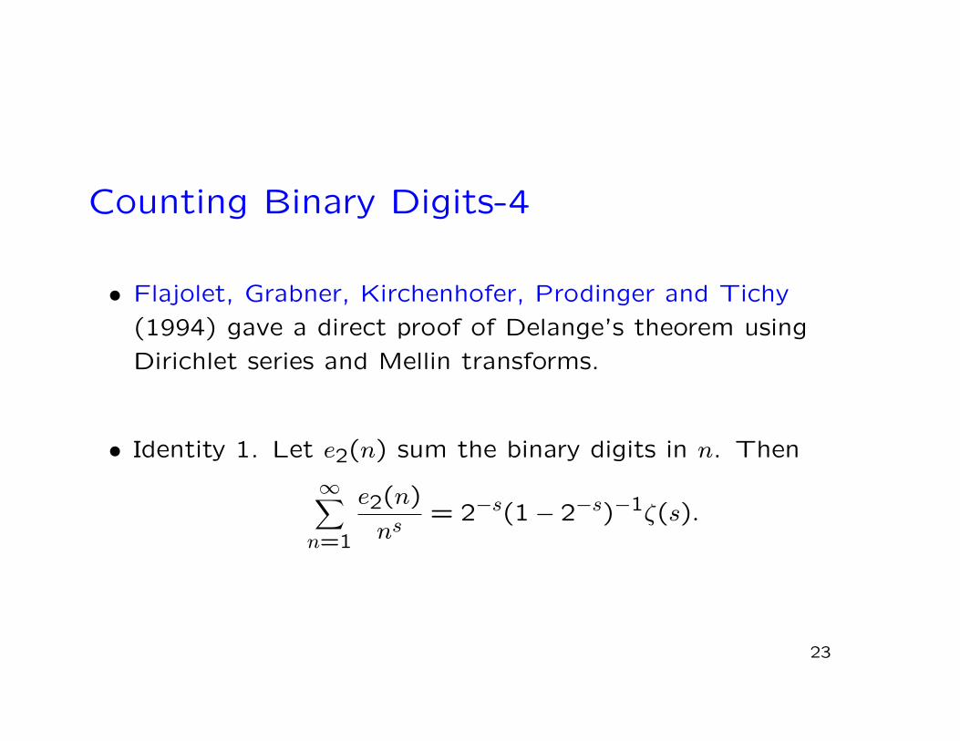
Counting Binary Digits-4

• Flajolet, Grabner, Kirchenhofer, Prodinger and Tichy(1994) gave a direct proof of Delange’s theorem usingDirichlet series and Mellin transforms.

• Identity 1. Let e2(n) sum the binary digits in n. Then

1X

n=1

e2(n)

ns= 2�s(1� 2�s)�1⇣(s).

23

Counting Binary Digits-5

• Identity 2: Special case of Perron’s Formula. Let

H(x) :=1

2⇡i

Z 2+i1

2�i1

⇣(s)

2s � 1xs ds

s(s� 1).

Then for integer N have an exact formula

H(N) =1

NS2(N)�

N � 1

2.

• Proof. Shift the contour to Re(s) = �14. Pick up

contributions of a double pole at s = 0 and simple poles ats = 2⇡ik

log 2, k 2 Z, k 6= 0. Miracle occurs: The shifted contourintegral vanishes for all integer values x = N . (It is a kindof step function, and does not vanish identically.)

24

Part III. Probability Theory: SingularFunctions

• Lomnicki and Ulam (1934) constructed singular functionsas solutions to various functional equations.

• Draw binary digits of a number, at random:0 with probability ↵

1 with probability 1� ↵.Let L↵(x) be the cumulative distribution function ofresulting distribution µ↵. Call this the Lebesgue functionwith parameter ↵.

25

Singular Functions-2

• These functions satisfy the functional equations (0 x 1),

L↵(x

2) = ↵ L↵(x),

L↵(x + 1

2) = ↵ + (1� ↵)L↵(x).

• Claim. The measure µ↵(x) = dL↵(x) is a (singular) measuresupported on a set of Hausdor↵ dimension

H2(↵) = �↵ log2 ↵� (1� ↵) log2(1� ↵).

(binary entropy function)

26

Singular Functions-3

• Salem (1943) determined the Fourier series of L↵(x). Heobtained it using

Z 1

0e2⇡itxdL↵(x) =

1Y

k=1

↵ + (1� ↵)e2⇡it2k

!

.

• Product formulas like this occur in wavelet theory (solutionsof dilation equations), see Daubechies and Lagarias (1991),(1992).

27

Singular Functions-4

• Theorem (Hata and Yamaguti 1984) For fixed x theLebesgue function L↵(x) extends in the variable ↵ to ananalytic function on the lens-shaped region

{↵ 2 C : |↵| < 1 and |1� ↵| < 1}.

The Takagi function appears as:

2 ⌧(x) =d

d↵L↵(x) |

↵=12

• Hata and Yamaguti, Japan J. Applied Math. 1 (1984),183-199. A very interesting paper!

28

Open Problem: Invariant Measure

• Observation The absolutely continuous measureµT := 2⌧(x)dx is a probability measure on [0,1].Call it the Takagi measure.

• General Query. Are there any interesting maps of theinterval f : [0,1]! [0,1] for which the Takagi measureµT (x) is an invariant measure?

29

Part IV. Analysis: Fluctuation Properties

• The Takagi function oscillates rapidly. It is an analysisproblem to understand the size of its fluctuations on variousscales.

• These problems have been completely answered, asfollows...

30

Fluctuation Properties: Single Fixed Scale

• The maximal oscillations at scale h are oforder: h log2

1h.

• Proposition. For all 0 < h < 1 the Takagi function satisfies

|⌧(x + h)� ⌧(x)| 2h log21

h.

• This bound is sharp within a multiplicative factor of 2.Kono (1987) showed that as h! 0 the constant goes to 1.

31

Maximal Asymptotic Fluctuation Size

• The asymptotic maximal fluctuations at scale h! 0 are oforder: h

q2 log2

1h log log log2

1h in the following sense.

• Theorem (Kono 1987) Let �l(h) =q

log21h. Then for all

x 2 (0,1),

lim suph!0+

⌧(x + h)� ⌧(x)

h �l(h)q

2 log log�l(h)= 1,

and

lim infh!0+

⌧(x + h)� ⌧(x)

h �l(h)q

2 log log�l(h)= �1.

32

Average Scaled Fluctuation Size

• Average Fluctuation size at scale h is Gaussian,proportional to h

qlog2

1h.

• Theorem (Gamkrelidze 1990) Let �l(h) =q

log21h. Then

for each real y,

limh!0+

Meas {x :⌧(x + h)� ⌧(x)

h �l(h) y} =

1p2⇡

Z y

�1e�

12t2dt.

• Kono’s result on maximum asymptotic fluctuation size isanalogous to the law of the iterated logarithm.

33

Part V. Rational Values

• Easy Fact.

(1) The Takagi function maps dyadic rational numbers k2n

to dyadic rational numbers ⌧( k2n) = k0

2n0 , where n0 n.

(2) The Takagi function maps rational numbers r = pq to

rational numbers ⌧(r) = p0q0. Here the denominator of ⌧(r)

may sometimes be larger than that of r.

• Next formulate three (hard?) unsolved problems...

34

Rational Values: Pre-Image Problems

• Problem 1. Determine whether a rational r0 has somerational preimage r with ⌧(r) = r0.

• Problem 2. Determine which rationals r0 have anuncountable level set L(r0).

• Problem 2 was raised by Donald Knuth (2004) in Volume 4of the Art of Mathematical Programming (Fascicle 3,Problem 83 in 7.2.1.3) He says:“WARNING: This problem can be addictive.”

35

Rational Values: Iteration Problems

• Problems 3 and 4. Determine the behavior of ⌧(x) underiteration, restricted to dyadic rational numbers, resp. allrational numbers.

• Remarks. (1) For dyadic rationals the denominators arenonincreasing, so all iterates go into periodic orbits. Butfiguring out orbit structure could be an interesting problem.

(2) For general rational numbers it is not clear whathappens. Denominators could potentially increase to +1.(Any invariant measure will be supported in [12, 2

3].)

36

Part VI. Level Sets of the Takagi Function

• Definition. The level set L(y) = {x : ⌧(x) = y}.

• Problem. How large are the level sets of the Takagifunction?

• Quantitative Problem. determine exact count if finite;determine Hausdor↵ dimension if infinite.

• Answer depends on sampling method: Could chooserandom x-values (abscissas) or random y-values (ordinates)

37

Size of Level Sets: Cardinality

• Fact. There exist levels y such that L(y) is finite,countable, or uncountable.

• L(15) is finite, containing two elements.

Knuth (2005) showed that L(15) = { 3459

87040, 8358187040}.

• L(12) is countably infinite.

• L(23) is uncountably infinite.

Baba (1984) observed this holds...because...

38

Size of Level Sets: Hausdor↵ Dimension

• Theorem (Baba 1984) The set L(23) has Hausdor↵

dimension 12.

• This result followed up by...

• Theorem (Maddock 2010) All level sets L(y) haveHausdor↵ dimension at most 0.699.

• Conjecture (Maddock 2010) All level sets L(y) haveHausdor↵ dimension at most 1

2.

39

Local Level Sets-1

• Approach to understand level sets: break them into locallevel sets, which are easier to understand.

• The local level set containing x is described completelyin terms of the binary expansion of x =

Pn�1 bn2�n.

• Definition. The deficient digit function Dn(x) counts theexcess of 0’s over 1’s in the first n digits of the binaryexpansion of x.

• For random x the values (D1(x), D2(x), D3(x), ...) are sumsof a simple random walk, taking steps +1 or �1.

40

Local Level Sets-2

• Given x, look at all the breakpoint values

0 = c0 < c1 < c2 < ...

where Dcj(x) = 0, i.e. values n where the random walkreturns to the origin. Call this set the breakpoint set Z(x).

• The binary expansion of x is broken into blocks of digitswith position cj < n cj+1. The flip operation exchangesdigits 0 and 1 inside a block.

• Definition. The local level set Llocx consists of all numbers

x0 ⇠ x by a (finite or infinite) set of flip operations. Allnumbers in Lloc

x have the same breakpoint set Z(x) = Z(x0).

41

Propeties of Local Level Sets

• Property 1. Llocx is a closed set.

• Property 2. Llocx is either a finite set of cardinality 2Z(x), if

there are finitely many blocks in Z(x), or is a Cantor setif there are infinitely many blocks in Z(x).

• Property 3. Each level set partitions into a disjoint union oflocal level sets.

42

Level Sets-Abscissa Viewpoint

• Problem. Draw a random point x uniformly with respect toLebesgue measure. How large is the level set L(⌧(x))?

• Partial Answer. At least as large as the local level set Llocx .

• Theorem A. For a randomly drawn point x, with probabilityone the local level set Lloc

x is an uncountable (Cantor) set ,of Hausdor↵ dimension 0.

43

Proof of Theorem A

(1) With probability one, the set of breakpoints Z(x) is infinite:the one-dimensional random walk Dn(x) returns to theorigin infinitely often almost surely. This makes Lloc

x aCantor set.

(2) With probability one, the expected time for the randomwalk Dn(x) to return to the origin is infinite. This “implies”that Lloc

x has Hausdor↵ dimension 0.

44

Number of Local Level Sets per Level

• Fact. The number of local level sets on a level can take anarbitrary integer value and also can be countably infinite.

• Theorem. There are a dense set of levels y such that L(y)contains a countably infinite number of local level sets.

• Known such levels all have y a dyadic rational, includingy = 1

2.

45

Level Sets-Abscissa View

• Problem.What is the average size of full level set L(⌧(x))where x is picked at random?

• This problem is unsolved. Expect the same answer asTheorem A: Most L(⌧(x)) uncountable of Hausdor↵ dim. 0.

• Di�culty. The mysterious problem is to understand howmany local level sets there are on a given level, when(abscissa) x is picked at random.

46

Expected Number of Local Level Sets:Ordinate View

• We are able to estimate the number of local level sets whenthe ordinate y is picked at random:

• Theorem B. The expected number of local level sets for an(ordinate) y drawn uniformly from 0 y 2/3 is finite.This number is exactly 3/2.

47

Level Sets-Ordinate view

• We can compute the expected size of a level set L(y) for arandom (ordinate) level y...

• Theorem C.(1) (Buczolich (2008)) The expected size of a level setL(y) for y drawn at random (Lebesgue measure) is finite.

(2) The expected number of elements in a level set L(y) fory drawn at random (Lebesgue measure) is infinite.

• Our proof of (1) di↵ers from the proof of Buczolich.It gives extra information, namely (2).

48

Local Level Sets: Size Paradox?

• Ordinate View: Level sets L(y) are finite with probability 1.

• Abscissa View: Level sets L(⌧(x)) are uncountably infinitewith probability 1.

• Reconciliation Mechanism: x-values preferentially selectlevel sets that are “large”.

49

Reconciling Size of Local Level Sets

• Theorem D. The set Big of levels y such that the level setL(y) has positive Hausdor↵ dimension, is itself a set of fullHausdor↵ dimension 1.

• Proof Idea. Explicit construction of local level sets givingdistinct y values having Hausdor↵ dimension > 1� ✏, for anygiven ✏ > 0.

50

Approach to Results

• We study the left hand endpoints of local level sets...

• Definition. The deficient digit set ⌦L is the set of left-handendpoints of all local level sets.

• Fact. The set ⌦L consists of all real numbers x whosebinary expansions have at least as many 0’s as 1’s after n

steps. That is, all Dn(x) � 0.(There is a unique choice of flips to achieve this.)

51

Approach to Results-cont’d.

• Key point. ⌦L keeps track of all local level sets. It is aclosed set obtained by removing a countable set of openintervals from [0,1]. It has has a Cantor set structure.

• Theorem E. ⌦L has Lebesgue measure 0 and has Hausdor↵dimension 1.

• This holds because...

52

Proof of Theorem E

• Heuristic Argument: Count the number of allowable stringsin expansions in ⌦L. There are about n�3/22n strings oflength n. The fact that

Pn�3/2 <1 implies Lebesgue

measure 0. The fact that allowed number exceeds 2(1�✏)n

“implies” deficient digit set ⌦L has Hausdor↵ dimension 1.

53

Flattened Takagi Function

• Restrict the Takagi function to ⌦L. On every open intervalthat was removed to construct ⌦L, linearly interpolate thisfunction between the two endpoints.

• Call the resulting function ⌧L(x) the flattened Takagifunction.

• Amazing Fact. (Or Trivial Fact.) All the linearinterpolations have slope �1.

54

Graph of Flattened Takagi Function

0.2 0.4 0.6 0.8 1.0

0.2

0.4

0.6

0.8

1.0

55

Flattened Takagi Function-2

• Claim. The flattened Takagi function has much lessoscillation than the Takagi function. Namely...

• Theorem F.(1) The flattened Takagi function ⌧L(x) isa function of bounded variation. That is, it is the sum ofan increasing function (means: nondecreasing) and adecreasing function (means: nonincreasing).(This is called: Jordan decomposition of BV function.)

(2) ⌧L(x)has total variation V 10 (⌧L) = 2.

• This theorem follows from...

56

Takagi Singular Function

• Theorem. (1) The flattened Takagi function has a minimalJordan decomposition

⌧L(x) = ⌧S(x) + (�x),

in which the function

⌧S(x) := ⌧L(x) + x

is nondecreasing, and the function �x is strictly decreasing.

(2) The function ⌧L(x) is a nondecreasing singularcontinuous function; it has derivative 0 o↵ the set ⌦L.Call it the Takagi singular function.

57

Graph of Takagi Singular Function

0.2 0.4 0.6 0.8 1.0

0.2

0.4

0.6

0.8

1.0

58

Takagi Singular Function

• The Takagi singular function is the integral of a singularmeasure:

⌧S(x) =Z x

0dµS(t)

Call µS the Takagi singular measure. It is supported on ⌦L.

• The Takagi singular measure is obviously nottranslation-invariant. But it satisfies various functionalequations coming from those of the Takagi function. It ispossible to compute with it.

59

Proof of Theorem B

• Compute expected value of number of local level sets atrandom level y using the co-Area formula for BV-functions,applied to ⌧L(x).

• This counts the expected number of points of the functionon each level. Exactly half of these endpoints correspond toleft hand endpoint of a level set. End up with answer 3

2.

60

Proof of Theorem C

(1) Compute the Takagi singular measure of various subsets of⌦L, those for which the breakpoint set Z(x) takes a finitevalue m � 1. Show that summing over 1 m <1 accountsfor all of the Takagi singular measure. This shows that, on⌦L only, drawing x with respect to Takagi singularmeasure, the number of points of ⌧L(x) = ⌧(x) is finite ona full measure set of ⌦L. Then carry this over to Lebesguemeasure on ordinates.

(2) Explicit computation of average value shows that thesesubsets also shows that the expected number of points isinfinite. QED

61

Concluding Remarks.

• Found interesting new internal structures: Takagi singularmeasure. Relation to random walks.

• Raised various open problems: Study the Conjugate Takagifunction U(✓). Study rational levels. Study Takagi functionas dynamical system (map of interval [0,1]).

62

The End

63