The Relevance of Magnetism for theDevelopment of Quantum Mechanics

Pascal Mauron - 2012.12.15

Contents

1 Introduction 1

2 Crookes tube and the discovery of the electron 22.1 Crookes tube . . . . . . . . . . . . . . . . . . . . . . . . . . . . . . . . . . . . . . 22.2 Thomson’s experiment . . . . . . . . . . . . . . . . . . . . . . . . . . . . . . . . . 32.3 Towards the Schrödinger equation . . . . . . . . . . . . . . . . . . . . . . . . . . 5

3 Quantization, spin, and the Stern-Gerlach Experiment 63.1 Black body radiation . . . . . . . . . . . . . . . . . . . . . . . . . . . . . . . . . . 63.2 The Bohr atom model . . . . . . . . . . . . . . . . . . . . . . . . . . . . . . . . . 63.3 The Stern-Gerlach experiment . . . . . . . . . . . . . . . . . . . . . . . . . . . . . 7

4 Degeneracy and the Zeeman effect 104.1 A brief refresher on the Hamiltonian for a central potential . . . . . . . . . . . . 114.2 The “normal” Zeeman effect . . . . . . . . . . . . . . . . . . . . . . . . . . . . . . 124.3 The g-factor . . . . . . . . . . . . . . . . . . . . . . . . . . . . . . . . . . . . . . . 134.4 The “anomalous” Zeeman effect . . . . . . . . . . . . . . . . . . . . . . . . . . . . 134.5 Spin-orbit interaction and the hydrogen fine and hyperfine structures . . . . . . . 15

1 Introduction

Towards the end of the nineteenth century, the achievements of what we today call classicalphysics were such that students were discouraged from this academic path on the reasoning thatall the important laws of physics had been discovered, meaning that research would only beconcerned with clearing minor problems or improving measurement methods [1].

The specificities of those minor problems can be found in any reference on the history ofphysics. This small paper focuses instead on the impact of phenomena of magnetic nature onthe development of quantum mechanics:• The discovery of the electron.• The experimental proof of the quantization of angular momentum.• The discovery of the electron spin.• The experimental proof of quantum degeneracy.

For the sake of completeness, phenomena that are not directly related to magnetism butwhere essential in the discovery of quantum mechanics are also briefly mentioned.

1

2 Crookes tube and the discovery of the electron

Wave–particle duality postulates that all particles exhibit both wave and particle properties.

The idea of duality originated in a debate that dates back to the 17th century. Competingtheories of light were proposed by Christiaan Huygens and Isaac Newton: light was thoughteither to consist of waves (Huygens) or of particles (Newton) [2].

Assuming light to travel at different speeds in different media, refraction could be easilyexplained as the medium-dependent propagation of light waves. The resulting Huygens–Fresnelprinciple was extremely successful at reproducing light’s behaviour and, subsequently supportedby Thomas Young’s discovery of double-slit interference, was the beginning of the end for theparticle light camp.

After James Clerk Maxwell discovered that only four equations are required to describeself-propagating waves of oscillating electric and magnetic field, it quickly became apparent thatvisible light, ultraviolet light, and infrared light (phenomena thought previously to be unrelated)were all electromagnetic waves of differing frequency. The wave theory had prevailed — or atleast it seemed to.

2.1 Crookes tube

Around 1870, cathode rays (revealed later to be streams of electrons) produced in a Crookestube1 were found to be deflected by both electric and magnetic fields, obeying Faraday-Henry’slaw of induction for currents in electric conductors [3].

∇×E = −∂B∂t

(1)

Figure 1: Electrons casting the shadow of a Maltese cross on the face of a Crookes tube(from [3]).

As was the case two centuries before, there were two opposed theories to explain whatwas happening [4]: cathode rays were either corpuscles (i.e. electrically charged atoms) oraether vibrations, some new form of electromagnetic waves that were separate from what carriedthe current through the partial vacuum of the tube. The debate continued until comparisons

1From the English physicist Sir William Crookes, also known as the inventor of the radiometer.

2

between experiments on cathode rays deflected by electric and magnetic fields allowed JosephJohn Thomson (1905 - Nobel Prize in Physics 1906) to measure the mass-to-charge ratio of avery light particle that was later named the electron.

2.2 Thomson’s experiment

This clever experiment (whose description here is freely adapted from an undergraduate labo-ratory course from Dartmouth University [5]) exploits the Lorentz interaction between electro-magnetic fields and charged particles.

F = q [E + v ×B] (2)

The apparatus consists in a Crookes tube where deflecting electric and magnetic fields can beapplied perpendicularly to each other (see Fig. 2), so that the electric and magnetic componentsof the Lorentz force are collinear:• The electric field is provided by two electrodes placed inside the tube.• The magnetic field (symbolised with a horseshoe magnet in the figure) is usually produced

with a Helmholtz coil.

Figure 2: Schematic view of the apparatus used in an experiment to determine the mass-to-charge ratio of electrons in a Crookes tube (from [5]).

2.2.1 Electron velocity

The first step is to determine the velocity of the particle. For this, both the magnetic and theelectric deflections are switched on, and the goal is to adjust them until the Lorentz force isas close to zero as possible. At this point the cathode rays follow straight lines again, as theywould without the external fields.

F = 0 ⇒ v =|E||B|

(3)

3

The amplitudes of both the electric and the magnetic fields can be computed from theconstruction details of the apparatus:• The amplitude of the electric field E depends on the voltage V applied between the

deflector plates separated by a distance d.• The amplitude of the magnetic field B is directly proportional to the current I circulating

in the Helmholtz coils.E =

V

dez

B = kHI ey

⇒ v =V

dkHI(4)

2.2.2 Mass-to-charge ratio of the electron

Between the electrodes is the electric field constant, meaning that if we now switch off themagnetic field, the cathode rays follow a parabolic curve.

ΣF = qE = ma (5)

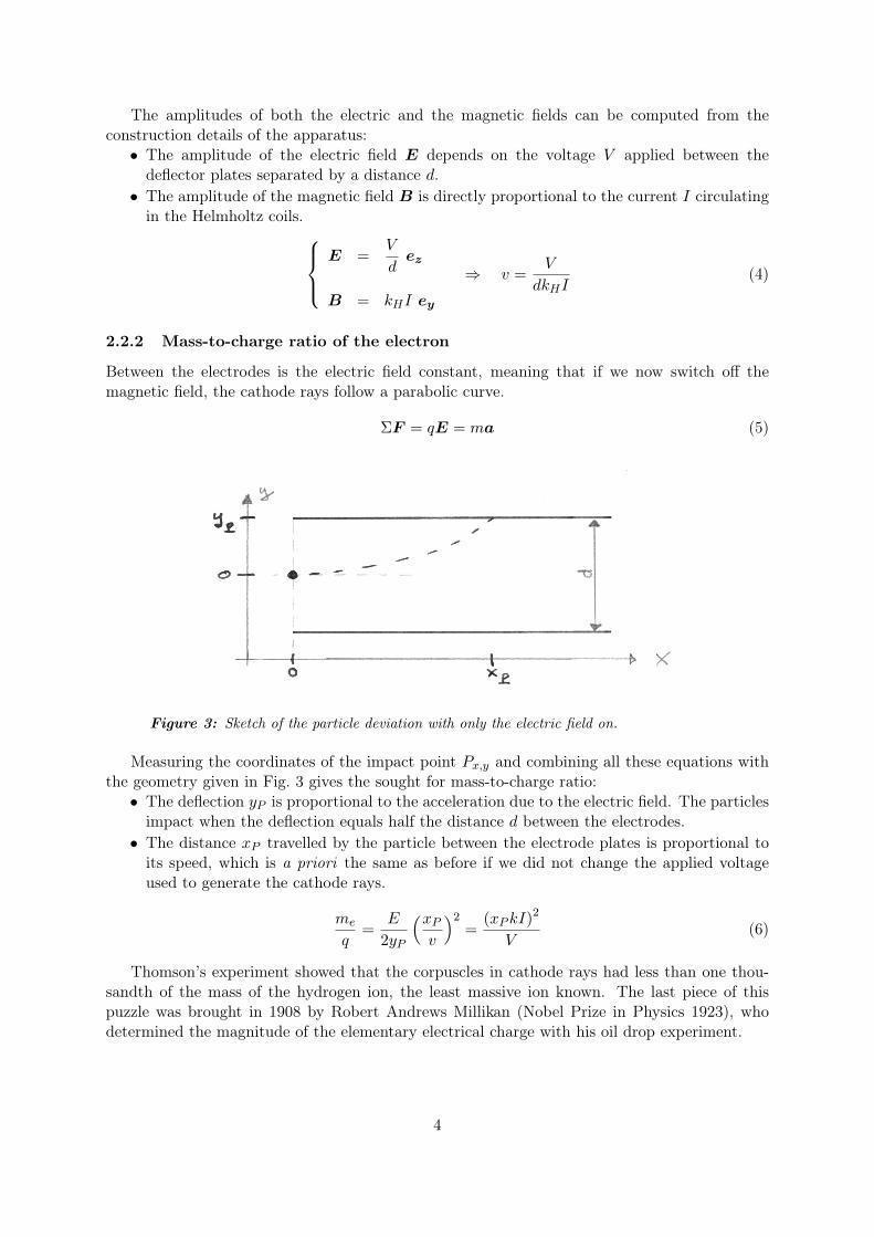
Figure 3: Sketch of the particle deviation with only the electric field on.

Measuring the coordinates of the impact point Px,y and combining all these equations withthe geometry given in Fig. 3 gives the sought for mass-to-charge ratio:• The deflection yP is proportional to the acceleration due to the electric field. The particles

impact when the deflection equals half the distance d between the electrodes.• The distance xP travelled by the particle between the electrode plates is proportional to

its speed, which is a priori the same as before if we did not change the applied voltageused to generate the cathode rays.

me

q=

E

2yP

(xPv

)2=

(xPkI)2

V(6)

Thomson’s experiment showed that the corpuscles in cathode rays had less than one thou-sandth of the mass of the hydrogen ion, the least massive ion known. The last piece of thispuzzle was brought in 1908 by Robert Andrews Millikan (Nobel Prize in Physics 1923), whodetermined the magnitude of the elementary electrical charge with his oil drop experiment.

4

2.3 Towards the Schrödinger equation

2.3.1 The planetary model of the atom

Thomson’s view of the atom was that of negatively charged plums (the electrons), surroundedby a positively charged pudding. To account for the electrical neutrality of atoms, the sum ofcharges was of course zero.

This was challenged by an experiment performed in 1908 by Hans Geiger and Ernest Marsden,under the guidance of Ernest Rutherford. When alpha particles were shot at a very thin gold foil,some of the exiting particles were deflected at high angles, which led Rutherford to formulate hisplanetary model of the atom (1911), based on Coulomb scattering between particles of opposedcharges.

Less than a decade later, Rutherford was the first to deliberately transmute one element intoanother: bombarding pure nitrogen with alpha particles produced oxygen and something newthat he identified as hydrogen nuclei. Hydrogen being known as the lightest element, Rutherfordpostulated this nucleus to be a new particle, which he dubbed the proton (1920) [6].

2.3.2 Compton scattering and de Broglie’s suggestion

Although classical electromagnetism predicted that the wavelength of scattered rays should beequal to the initial wavelength, multiple experiments had found that it was in fact longer (i.e.corresponding to lower energy).

In 1923, Arthur Holly Compton (Nobel Prize in Physics 1927) explained this shift by at-tributing particle-like momentum to Einstein’s photons, by assuming that each photon interactedwith only one electron. Conservation of mass-energy and momentum leads to a wavelength shiftthat depends on the mass of the impacted particle and on the scattering angle.

The same year, Louis de Broglie (Nobel Prize in Physics 1929), guided by the analogy ofFermat’s principle in optics, was led to suggest that the dual wave-particle nature of radiationshould have its counterpart in a dual particle-wave nature of matter. His expression relatingthe wave vector k and the momentum p of a particle was verified through the observation ofelectron diffraction by a crystal lattice [7].

p = ~ · k (7)

Figure 4: Sketch (left, from [8]) and example (right, from [9]) of electron diffraction.

5

2.3.3 The Schrödinger equation

In view of the consequences and achievements of quantum mechanics, the next steps are sur-prisingly straightforward. Considering the kinetic and radiative energy of a wave-like particle tobe identical

E = ~ω =p2

2m(8)

and using these definitions for a wave function ψ

ψ (x, t) = ψ0 ej(kx−ωt) = ψ0 e

j~ (px−Et) (9)

directly2 leads to the well-known Schrödinger equation.

E ψ (x, t) = j~∂

∂tψ (x, t) = − ~2

2m

∂2

∂x2ψ (x, t) (10)

3 Quantization, spin, and the Stern-Gerlach Experiment

According to the Bohr–van Leeuwen theorem of statistical mechanics, the thermal average ofthe magnetization is always zero3. This makes magnetism in solids solely a quantum mechanicaleffect that cannot be accounted for by classical physics [10]. Only quantization allows to solvethe discrepancy between theory and experimentation.

3.1 Black body radiation

In 1900, John William Strutt (3rd Baron Rayleigh, Nobel Prize in Physics 1904) and JamesJeans presented a derivation of the energy density u of a black body, based on the equipartitionof energy over all possible oscillators of angular frequency ω at a temperature T . Alas, theRayleigh-Jeans law is known for predicting the so-called ultraviolet catastrophe: the energyoutput should diverge towards infinity as wavelength approaches zero.

This dilemma was solved the same year by Max Planck (Nobel Prize in Physics 1918), byassuming that the resonators considered using Boltzmann’s statistics could only emit energy inquantized form, as a multiple of the elementary unit energy E0 = ~ω0.

En = nE0 = n~ω0 , n ∈ N∗ (11)

Due to this quantization, calculation of the partition function of the system is done with asummation instead of an integral, which removes the divergence at high frequencies.

3.2 The Bohr atom model

Rutherford’s planetary model of the atom that we mentioned before faced insurmountable dif-ficulties. Following the Larmor equation of classical electrodynamic, an electron in orbit shouldcontinuously radiate energy, and one can estimate that it would take it approximately 10−10 sto spiral into the nucleus from an orbit of the size of 10−10 m [7]. Furthermore, an electron inperiodic motion around an atom nucleus should radiate with the same frequency as that motion.

2Of course, we neglect here the fact that the spatial derivative is actually an operator.3 The intuitive proof is that the rate of work W done by the Lorentz force F on a particle with charge q and

velocity v does not depend on the magnetic field B.

W = F · v = q (E + v ×B) · v = qE · v

6

This was in clear disagreement with experimental results that a) some atoms are stable (!) andb) they emit light only in very narrow bands.

Along the same lines as Planck’s hypothesis of quantized energy levels of a resonator, NielsBohr (Nobel Prize in Physics 1922) postulated in 1913 that an atom may only exist in statesof discrete energy levels, the difference of which should correspond to the emission spectrum ofthe atom, thus avoiding the radiation allowed by a continuous energy spectrum [11].

ω =∆E

~(12)

Applying classical mechanics to this problem leads to a quantization of the angular momen-tum L, in units of ~, where n is called the primary quantum number.

L = n~ , n ∈ N∗ (13)

From this condition we can calculate two widely used constants pertaining to the hydrogenatom: the Bohr-radius a0, which corresponds to the radius of the lowest orbit of a planetaryelectron of mass me (ground state n = 1), and the Rydberg constant Ry, which gives the energylevel for the state n.

a0 =~2

mee2= 0, 529 · 10−10 m (14)

En = −Ry 1

n2(15)

Ry =mee

4

2~2= 13, 606 eV (16)

The Bohr atom model was very successful for hydrogen or helium, being able to explainthe Rydberg formula for the spectral emission lines of atomic hydrogen. But it was unable toexplain more complex effects such the Zeeman effect or the fine structure, which we will discusslater in more detail.

3.3 The Stern-Gerlach experiment

In 1922, Otto Stern and Walter Gerlach designed an experiment to test the quantization ofangular momentum (also known as Bohr-Sommerfeld quantization) [7] [12]. A beam of electri-cally neutral silver atoms was directed through an inhomogeneous magnetic field B, with theapparatus described in Fig. 5.

Figure 5: Schematic view of the Stern-Gerlach experiment (from [12] and [7]).

7

The magnetic moment µ produced by an electric charge q moving along a circular pathof radius r depends on its instantaneous velocity v. Consequently, the magnetic moment is afunction of the angular momentum L.

µ =1

2q r × v =

q

2mL (17)

Figure 6: Magnetic moment of a charged particle in orbit, from [8].

Eq. 17 is the base of the definition of the Bohr magneton µB, which is the magnetic momentof an electron of mass me at the lowest possible angular momentum L = ~.

µB =e

2me~ (18)

The interaction of a magnetic moment µ with a magnetic field B gives rise to a change inenergy V

V = −µ ·B (19)

and thus a forceF on the atom.

F = −∇V = ∇ {µxBx + µyBy + µzBz} (20)

With the magnetic field primarily pointing in the z-direction, precession of the magneticmoment about this same axis4 is sufficiently fast for the average values of µx and µy to vanish.Thus the (average) net force points only in the z direction, leading to a deviation of the particleproportional to the angular momentum and the gradient of the magnetic field.

Fz = µz∂B

∂z=

q

2m

∂B

∂zLz (21)

4 Known as the Larmor precession, which for a (classical) electron is characterised by a frequency of over10 GHz/Tesla.

L =q

2mL×B =

q

2mBL× ez ⇒ ωLarmor =

q

2mB

8

The experiment was carried out with a beam of silver atoms from a hot oven impactingon a target. Silver atoms were chosen because all shells are complete up to a single outerelectron5. Thus the sum of the angular momentums of all the inner electrons is zero (Hund’srule for spatial symmetry), meaning that this large atom acts magnetically as a single electron.Furthermore, this single electron has zero orbital angular momentum (5s1 with orbital quan-tum number l = 0): one would expect there to be no interaction with an external magnetic field6

Figure 7: Gerlach’s postcard to Niels Bohr, dated February 8th, 1922.

Stern and Gerlach’s experimental results rose two questions [13] that could not be answeredclassically:• Although this electron has actually zero angular momentum, it behaves as if it possessed

a magnetic moment, which could only be the result of some current loop.• Instead of the continuous smear that would be produced by all possible orientations of

the dipoles, the target revealed that the field separated the beam into two distinct parts,indicating a quantization of this newly discovered magnetic moment of the electron.

In 1924, Wolfgang Pauli (Nobel Prize in Physics 1945) proposed a new quantum degreeof freedom (or quantum number) with two possible values, in order to resolve inconsistenciesbetween observed molecular spectra and the developing theory of quantum mechanics. Heformulated the Pauli exclusion principle, perhaps his most important work, which stated thatno two electrons could exist in the same quantum state, identified by four quantum numbersincluding his new two-valued degree of freedom.

The idea of spin originated with Ralph Kronig. In 1925, Samuel Abraham Goudsmit andGeorge Eugene Uhlenbeck postulated that the electron had an intrinsic angular momentum, in-dependent of its orbital characteristics. In classical terms, a ball of charge could have a magneticmoment if it were spinning such that the charge at the edges produced an effective current loop.This kind of reasoning led to the use of the name electron spin to describe the intrinsic angularmomentum, as if the electron were a spinning ball of charge.

5 The use of silver also proved to be fortuitous, as the high sulfur content of Stern’s bad cigar turned the silveratoms deposited on the target to silver sulfide, which was similar to developing a photographic film [14].

6 The set of orthogonal systems known as spherical harmonics had been studied by Pierre-Simon de Laplaceat the end of the 18th century, and the existence of the quantum numbers l emerged from a discussion of ellipticalorbits based on the Bohr atom theory. Finally, the shell terminology comes from Arnold Sommerfeld (of theBohr-Sommerfeld quantization), and their existence was confirmed by X-ray diffraction experiments performedin 1913 [15].

9

This picture of the rotation of a particle around some axis is correct so far as spins obeythe same mathematical laws as quantized angular momenta do7. However, this “spinning ball”picture is not realistic: the electron should be rotating so fast that its radius would move fasterthan light. The spin is simply another degree of freedom available to this particle. Spins alsopossess some peculiar properties that distinguish them from orbital angular momenta [16]:• The spin quantum numbers may take on half-odd-integer values.• Although the direction of its spin can be changed, an elementary particle cannot be made

to spin faster or slower.• The spin of a charged particle is associated with a magnetic dipole moment µs with ag-factor differing from 1 (which we will discuss later). This could only occur classically ifthe internal charge of the particle were distributed differently from its mass.

4 Degeneracy and the Zeeman effect

In 1896, Dutch physicist Pieter Zeeman (Nobel Prize in Physics 1902) discovered what we callnow the Zeeman effect : the splitting of spectral lines by a strong magnetic field8.

Historically, one distinguishes between the “normal” and one “anomalous” Zeeman effects.Both have actually the same cause, but there was no good explanation for the “anomalous” oneuntil the discovery of the electron spin.

Figure 8: One of the applications of the (“normal”) Zeeman effect: the magnetic field ofa sunspot is proportional to the splitting of the hydrogen line (from [18]).

7 The total angular momentum J is the vector sum of the orbital angular momentum L and of the intrinsicspin momentum S, using the Clebsch-Gordan coefficients.

8 The explanation came from his compatriot Hendrik Lorentz (with whom he shared the Nobel Prize), whodescribed the polarization of the light emitted by a excited charged particle in the presence of a magnetic field.Still a few years before Thomson’s discovery of the electron, Zeeman’s work showed that the particles had to benegatively charged and a thousandfold lighter than the hydrogen atom [17].

10

4.1 A brief refresher on the Hamiltonian for a central potential

In the three-dimensional case, the time-independent Schrödinger equation for a central potential(from a nucleus with charge Ze and a single electron) in spherical coordinates takes the form9

− ~2

2m

(∂2

∂r2+

2

r

∂

∂r

)ψ (r) +

L2

2mr2ψ (r) + V (r)ψ (r) = E ψ (r) (22)

This allows to separate the variables of the corresponding wave function ψ (r) into a radialpart Rnl(r) and an angular part Ylml

(θ, φ) (spherical harmonics).

ψ (r) = Rnl(r)Ylml(θ, φ) (23)

Ylml(θ, φ) are eigenfunctions of the square of the operator of angular momentum L2, and as

this operator commutes with the Hamiltonian and with one of its components (usually chosento be Lz)10, all three operators H, L2 and Lz have a (complete) set of common eigenstates.

These eigenstates are characterised by a set of parameters [19]:• The primary quantum number n describes the electron shell of the atom (energy level).• The azimuthal quantum number l describes the subshell (named s for l = 0 then p, d, f,

g...), giving the magnitude of the angular momentum.• The magnetic quantum number ml yields the projection of the angular momentum along

a specified axis.• The introduction of spin adds a fourth parameter: the spin projection quantum numberms.

En = − m

2n2

(Ze2

~

)2

L2 = ~2 l(l + 1)

Lz = ~ ml

Sz = ~ ms

(24)

The allowed energy states En are the same as with the Bohr model, but because of the wavefunction we can map out the probability distribution for the electron without having to rely onclassical orbits. Furthermore, while the energy levels are characterised by the primary quantumnumber n, the mathematical derivation shows that there are really two quantum numbers.

n = nr + l + 1

{n ∈ N∗

l ∈ N (25)

Finally, for each eigenvalue l there are actually (2l + 1) different eigenfunctions of quantumnumber ml, for a total of n2 levels of degeneracy.

− l ≥ ml ≥ l ,ml ∈ N (26)

n−1∑l=0

(2l + 1) = n2 (27)

9Where m = m1m2m1+m2

is actually the reduced mass.10Conservation of energy and momentum!

11

The underlying mathematics for spin are the same as for the projection of the angularmomentum, meaning that an electron with spin s = 1

2 actually doubles the level of degeneracyto 2n2.

− s ≥ ms ≥ s ,ms = ±1

2(28)

4.2 The “normal” Zeeman effect

The Hamiltonian H of an atom in a magnetic field can be given as the sum of the unperturbedHamiltonian of the atom H0 and of the perturbation HB due to the magnetic field.

H = H0 +HB (29)

As already exposed while discussing the Stern-Gerlach experiment, the perturbation is pro-portional to the projection of the magnetic moment µ on the magnetic field B.

HB = −µ ·B =e

2meL ·B (30)

Due to the separation of variables, only theml eigenvalues to the z-component of the angularmomentum are of interest here.

∆Enlml= 〈nlml|HB|nlml〉 =

eB

2me〈nlml|Lz|nlml〉 =

e~2me

B ml (31)

The magnetic field breaks the degeneracy, giving rise to (2l + 1) energy shifts of magni-tude ∆Enlml

, known as the Zeeman effect. For hydrogen and a magnetic field of 1 Tesla, theshift corresponds to 58 µeV .

Figure 9: Zeeman splitting of the 6-fold degeneracy of the p-state of the hydrogen atom(from [8]). The angular momentum produces a triplet (ml ∈ ±1) with twofolddegeneracies due to spin. The value of gS ≈ 2 compensates the half-integralspin angular momentum, and the result is a quintuplet with twofold degeneracyof the central state.

12

4.3 The g-factor

When the Zeeman effect was observed for hydrogen, the observed splitting was consistent withan electron orbit magnetic moment given by [13]

µorbital = − e

2meL = −µB

~L (32)

But when the effects of electron spin were discovered by Goudsmit and Uhlenbeck, they foundthat the observed spectral features were matched by assigning to the electron spin a magneticmoment

µspin = −gSe

2meS (33)

where gS is the electron spin g-factor.

A g-factor is a dimensionless quantity which characterizes the magnetic moment of a particleor nucleus. It is a proportionality constant that relates the observed magnetic moment µ to theappropriate angular momentum, usually in units of the Bohr magneton [20].

Any particle having a magnetic moment has an associated g-factor: protons, neutrons,muons, nuclei. The g-factor has a direct influence on the Larmor precession, and the associateddifferences between nuclei are the basis for magnetic resonance.

More precise experiments showed that the value was slightly greater than 2, and this fact tookon added importance when that departure from 2 was predicted by quantum electrodynamics.In fact, the value of gS has been determined to be [8]

gS = 2.0023193043622(15) (34)

and is one of the most precisely known values in all physics.

4.4 The “anomalous” Zeeman effect

The normal Zeeman effect only accounts for an odd number of lines. The presence of evennumber of lines that could be irregularly separated as well was a mystery until the discovery ofspin [7]. Because of spin, the level of degeneracy doubles and the new perturbation HB leads toa slightly different expression for the energy shift.

HB =e

2me(L+ gSS) ·B (35)

The key to this new problem is the rule of vector addition of two quantum-mechanical angularmomenta, established by Alfred Landé in 1920-1921. Accordingly, we calculate the eigenstatesof J2 and Jz (with quantum numbers j and mj , respectively11), where J = L + S is the totalangular momentum.

For an electron with gS ≈ 2 and a magnetic magnetic field B defined along the z-axis, weneed to calculate

eB

2me〈jmjl|Lz + 2Sz|jmjl〉 ≈

eB

2me〈jmjl|Jz + Sz|jmjl〉 (36)

11 These quantum numbers define the same kind of eigenstates as given in Eq. 24 for the angular momentum L.

13

Eq. 36 is linear, and the first term is easy to calculate.eB

2me〈jmjl|Jz|jmjl〉 =

e~2me

B mj (37)

The problem with the second term is that J is a constant of the motion, while S and L arenot. As a consequence, both S and L precess around J (see Fig. 10). As with the Stern-Gerlachexperiment, this precession is fast enough for us to have to consider only their average values,which are their respective projections onto J .

Figure 10: Precession of the angular momentum L and magnetic momentum S aroundthe total angular momentum J (from [7]).

〈S〉 =S · JJ2 J =

S · J~2j(j + 1)

J (38)

Using L = J − S and squaring on both sides,

S · J =1

2

[J2 + S2 −L2

]=

~2

2[j(j + 1) + s(s+ 1)− l(l + 1)] (39)

we can now define Sz as a function of Jz.

〈Sz〉 = 〈Jz〉j(j + 1) + s(s+ 1)− l(l + 1)

2j(j + 1)(40)

Adding Eq. 37 and 40 with(s = 1

2

)and

(j = l ± s = l ± 1

2

)gives the sought for energy shifts.

The term in parentheses is known as the Landé g-factor gj . Fig. 11 gives a general representationof the anomalous Zeeman effect.

∆EZ = mje~

2meB

(1± l

2l + 1

)= mj

e~2me

B gj (41)

gj =

2l + 2

2l + 1

2l

2l + 1

(42)

If the external field is strong enough so that the spin-orbit coupling can be neglected, Eq. 41can be simplified for hydrogen to Eq. 43, which gives the Zeeman splitting shown in Fig. 9.

∆EZ =e~

2meB (ml + 2ms) (43)

14

Figure 11: General representation of the anomalous Zeeman effect (from [7]).

4.5 Spin-orbit interaction and the hydrogen fine and hyperfine structures

Further interactions are all actually variants of the Zeeman effect: some magnetic moment andcharges in relative movement to each other. The mathematical treatments are in essence thesame as presented for the anomalous Zeeman effect. In order to keep this paper small, theseeffects are only discussed in broad terms.

4.5.1 Spin-orbit interaction

The Stern-Gerlach experiment was not the only experimental evidence that suggested an ad-ditional property of the electron. The other was the closely spaced splitting of the hydrogenspectral lines, called fine structure, which is caused by the phenomenon called spin-orbit coupling.

We have already seen how an external magnetic field affects the Hamiltonian of an electronin a central potential. But because of the intrinsic magnetic momentum known as spin, thisspin-orbit coupling acts like a permanent Zeeman effect due to the magnetic field generated bythe moving electrons.

Ignoring relativistic effects, the magnetic field generated by the electron depends on theelectric field E and on the velocity of the particle, i.e. its momentum L, according to theMaxwell equations. Assuming a central potential V (r), this can be expressed as

B = −v ×Ec2

=L

mec2

∣∣∣∣Er∣∣∣∣ =

1

c2v × r

r

dV (r)

dr(44)

µ = − e

2megSS (45)

The interaction with the intrinsic magnetic moment corresponds to a spin-orbit perturba-tion HSO, given here for a point of charge Ze interacting with a single electron. The reductionby a prefactor of 2 comes from relativistic effects known as Thomas precession [7]. It correspondsto an internal magnetic field on the electron of about 0.4 Tesla [13].

HSO = −µ ·B = −1

2·[

e

m2ec

2S ·L1

r

dV

dr

]=

Ze2

4πε0

1

2m2ec

2

S ·Lr3

(46)

15

Figure 12: Schematic representation of the hydrogen fine structure due to spin-orbit in-teraction (from [13]).

4.5.2 The hyperfine structure

The last effect we will discuss (even if very briefly) is the very tiny hyperfine splitting, which isa permanent Zeeman effect due to the magnetic field generated by the magnetic dipole momentof the nucleus.

If the spin operator of the nucleus is denoted by I, then the magnetic dipole operator is

M =Z e gN2MN

I (47)

where Z is the nuclear charge, MN the nuclear mass, and gN its gyromagnetic ratio (g-factor).

The hyperfine structure is a factor me/MN smaller than the typical spin-orbit coupling.

Figure 13: Schematic representation of the hydrogen hyperfine structure due to interac-tion between the total angular momentum of the electron and the magneticdipole moment of the nucleus (from [13]).

16

References

[1] Wikipedia, http://en.wikipedia.org/wiki/History_of_physics, Status December 2012

[2] Wikipedia, http://en.wikipedia.org/wiki/Wave-particle_duality, Status December2012

[3] Wikipedia, http://en.wikipedia.org/wiki/Crookes_tube, Status December 2012

[4] Wikipedia, http://en.wikipedia.org/wiki/J._J._Thomson, Status December 2012

[5] Undergraduate physics laboratory of Dartmouth University, http://www.dartmouth.edu/~phys1/labs/lab3.pdf, Status December 2012

[6] Wikipedia, http://en.wikipedia.org/wiki/Ernest_Rutherford, Status December 2012

[7] Stefan Gasiorowicz, Quantum Physics, 3rd edition, John Wiley & Sons, 2003

[8] Matthias R. Gaberdiel, Quantenmechanik I, Skript zur Vorlesung der ETH Zürich, Win-tersemester 2006-2007

[9] Wikipedia, http://en.wikipedia.org/wiki/Electron_diffraction, Status December2012

[10] Wikipedia, http://en.wikipedia.org/wiki/Bohr-van_Leeuwen_theorem, Status Decem-ber 2012

[11] Wikipedia, http://en.wikipedia.org/wiki/Bohr_model, Status December 2012

[12] Wikipedia, http://en.wikipedia.org/wiki/Stern_gerlach, Status December 2012

[13] HyperPhysics at the Georgia State University, http://hyperphysics.phy-astr.gsu.edu/hbase/hframe.html, Status December 2012

[14] Bretislav Friedrich and Dudley Herschbach, Stern and Gerlach: how a bad cigar helpedreorient atomic physics, Physics Today 56, 53, December 2003

[15] Wikipedia, http://en.wikipedia.org/wiki/Electron_shell, Status December 2012

[16] Wikipedia, http://en.wikipedia.org/wiki/Spin_quantum_number, Status December2012

[17] Wikipedia, http://en.wikipedia.org/wiki/Pieter_Zeeman, Status December 2012

[18] Sami K. Solanki, http://www.mps.mpg.de/homes/solanki/saas_fee_39/SaasFee39_Handout_L1.pdf, Max Planck Institute for Solar System Research, Saas-Fee AdvancedCourse 39, 2009

[19] Wikipedia, http://en.wikipedia.org/wiki/Quantum_number, Status December 2012

[20] Wikipedia, http://en.wikipedia.org/wiki/G-factor_(physics), Status December 2012

17