The Promises and Pitfalls of Factor Timing · The Promises and Pitfalls of Factor Timing April 2017 J. Bender X. Sun R. Thomas V. Zdorovtsov Abstract: The potential to dynamically

Information Classification: General

1

The Promises and Pitfalls of Factor Timing

April 2017

J. Bender

X. Sun

R. Thomas

V. Zdorovtsov

Abstract:

The potential to dynamically allocate across factors, “factor timing,” has been an area of academic and

practitioner research for decades. In this paper, we revisit the promises of factor timing, documenting

the historical linkages between equity factor performance and different groupings of predictors—

Sentiment, Valuation, Trend, Economic Conditions, and Financial Conditions. We highlight that different

predictors are more relevant for certain horizons so in factor timing, the horizon is critical. We also

argue there are significant pitfalls with factor timing as well. The difficulty of timing factors has been

well-documented, given the uncertainty of exogenous elements affecting their behavior and the

complexity of the underlying relationships. Most importantly, the underlying causal links are time-

varying. In addition, these relationships are observed with the benefit of hindsight, and thus suffer

from the age-old problem of data mining. However, we believe at the margin it is possible to time

certain elements that can add value and improve outcomes.


I. Introduction: Why Time Factors?

Factor research has been deeply ingrained in the academic asset pricing literature since the early days of

financial theory. The notion that certain stock characteristics or “factors” drive stock returns underlies

modern quantitative investing and risk modeling. Ross (1976) was among the first to note that one way

to understand the returns to stocks was to model them as a function of exposures to various factors. A

factor can be viewed as an attribute relating a set of securities’ returns. While a wide range of factors

have been proposed (macroeconomic factors, statistical factors, and fundamental factors, to name a

few), the most widely cited today are Value, Size, Momentum, Low Volatility, Quality, and Liquidity.

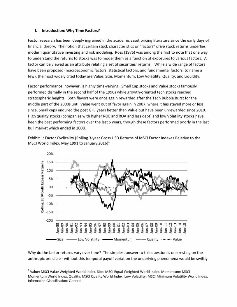
Factor performance, however, is highly time-varying. Small Cap stocks and Value stocks famously

performed dismally in the second half of the 1990s while growth-oriented tech stocks reached

stratospheric heights. Both flavors were once again rewarded after the Tech Bubble Burst for the

middle part of the 2000s until Value went out of favor again in 2007, where it has stayed more or less

since. Small caps endured the post GFC years better than Value but have been unrewarded since 2010.

High quality stocks (companies with higher ROE and ROA and less debt) and low Volatility stocks have

been the best performing factors over the last 5 years, though these factors performed poorly in the last

bull market which ended in 2008.

Exhibit 1: Factor Cyclicality (Rolling 3-year Gross USD Returns of MSCI Factor Indexes Relative to the MSCI World Index, May 1991 to January 2016)1

Why do the factor returns vary over time? The simplest answer to this question is one resting on the

anthropic principle - without this temporal payoff variation the underlying phenomena would be swiftly

1 Value: MSCI Value Weighted World Index. Size: MSCI Equal Weighted World Index. Momentum: MSCI

Momentum World Index. Quality: MSCI Quality World Index. Low Volatility: MSCI Minimum Volatility World Index.

-20%

-15%

-10%

-5%

0%

5%

10%

15%

20%

Jun

-88

Jun

-89

Jun

-90

Jun

-91

Jun

-92

Jun

-93

Jun

-94

Jun

-95

Jun

-96

Jun

-97

Jun

-98

Jun

-99

Jun

-00

Jun

-01

Jun

-02

Jun

-03

Jun

-04

Jun

-05

Jun

-06

Jun

-07

Jun

-08

Jun

-09

Jun

-10

Jun

-11

Jun

-12

Jun

-13

Jun

-14

Jun

-15

Ro

llin

g 3

6 M

on

th E

xce

ss R

etu

rns

Size Low Volatility Momentum Quality Value


3

arbitraged away. The factors wouldn’t exist to begin with. To understand the different undercurrents

affecting realized factor returns, it helps to decompose the premia into their key components.

Although the relative magnitudes differ across factors, the main ingredients of each factor’s premium

are (1) compensation for exposure to risk; (2) the return originating from irrationality of market

participants; and (3) the effects of market frictions. Intuitively, each of these may have its own

dynamics over time and its own drivers. For example, as levels of (and/or tolerance to) a specific source

of risk wax and wane, the realized return to bearing an exposure to that risk will move accordingly.

Similarly, the extent to which markets overreact, underreact, or manifest other irrational behaviors that

lead to systematic mispricings will vary over time, as will the degree to which market frictions slow down

or distort the process of price discovery (e.g. think of introductions and removals of restrictions on short

selling etc.)

While these dynamics highlight the benefits of diversification – and indeed multifactor models are a

staple in asset management for this very reason – they also hint at both the limitations of diversification

and the opportunity to improve upon it. Take the risk premium component of factor returns for

example. Clearly, extreme realizations of either level or price of any presumably orthogonal source of

risk will tend to spill over into other theretofore independent premia – just as a big hurricane might

impact both flood and auto-insurance claim incidence as well as the pricing of those policies. What this

means is that factor diversification tends to under-deliver when it’s needed the most - in top-down

driven environments when correlations between factors tend to become more pronounced.

On the positive side however, the rich dynamics of the drivers of factor premia and their core

components may provide an opportunity to improve upon a static factor allocation and, on margin, to

weather the storms a little better.2

Is factor timing possible? If so, we can improve upon the performance of holding a fixed weighted

basket of various factor portfolios. In the remainder of this paper, we look at whether this holy grail of

factor investing has merit. In Section II, we review what the academic literature has to say about factor

prediction. In Section III, we lay out the different predictors that have been proposed by academics and

practitioners, assessing the investment rationale behind each one. Section IV presents the empirical

evidence—which signals historically appear to predict future factor performance. In Section V, we

highlight the perils of using the empirical evidence to predict future factor performance and discuss the

challenges with building factor timing models. Lastly, we conclude with our observations around several

candidate approaches to building a factor timing model.

2 A digression is in order. Because correlations among factors ebb and flow over time around long-run averages, a

static process with fixed nominal weights to these themes will see the effective weights and portfolio exposures to said themes oscillate and do so quite meaningfully over time. As a result, managers with static approaches are in reality still “timing” factors and arguably doing so in a less informed way than might be attained by explicit factor forecasting approaches.


II. The Literature

What does the academic literature have to say about factor prediction? To start, there is a large body of

work around what predicts aggregate market equity returns. Campbell and Shiller (1998)3 found

evidence that the CAPE ratio (cyclically adjusted price-to-earnings ratio) could predict long-term (10-

year ahead) aggregate equity returns. The rationale was based on simple mean-reversion in stock

prices; abnormally high stock prices (relative to earnings) would eventually fall in the future to bring the

ratios back to more normal historical levels.4 The Campbell and Shiller model remains a seminal model

for forecasting long-term equity returns to this day. Subsequent papers focused on whether markets

could be timed at shorter horizons. Huang et al. (2014) presented compelling evidence that “sentiment”

indicators could be predictive at 1-month horizons. Other predictors that have been proposed include

the aggregate market’s implied cost of capital (Li, Ng, and Swaminathan (2013), stock market volatility

(Merton (1980), French, Schwert and Stambaugh (1987), the share of equity issues in total new equity

and debt issues (Baker and Wurgler, 2000), spread between yields on low-grade corporate bonds and

one-month Treasury Bills (Keim and Stambaugh, 1986), historical real earnings (Campbell and Shiller,

1988), dividend yield (Fama and French, 1988), cross-sectional beta premium (Polk et al. 2006), Term

spread (Campbell 1987 and Fama and French 1989), inflation (Campbell and Vuolteenaho, 2003), and

investment to capital ratio (Cochrane, 1991)).

In the area of factor prediction, many of the aforementioned predictors for the aggregate equity market

have been tested by practitioners, but the current literature, particularly by academics, remains sparse.

(This is not altogether surprising given that a considerable amount of debate continues in academia

around the very existence of these factors.) The research that does exist looks at a wide variety of

predictors, from market and sentiment indicators to macroeconomic indicators.5

Valuation: Extending Campbell and Shiller’s framework to factors has been one vein of

research. For instance, Garcia-Feijoo, Kochard, Sullivan, Wang (2015) corroborate Campbell and

Shiller’s evidence with low-risk strategies, showing that these strategies historically

outperformed more reliably in periods subsequent to low-beta stocks exhibiting relatively high

B/P levels, and even more so if they subsequently load positively on momentum. The authors

take great care in what the implications of these findings are; they are cautious (in our minds,

rightfully so) that the results mean investors should consider how valuation and momentum

interact with low-risk portfolios over time.

3 “Valuation Ratios and the Long-Run Stock Market Outlook,” Journal of Portfolio Management

4 Around the same time, the controversial Fed Model became popular, a rule of thumb that equities were

attractive when the market’s earnings yield was higher than the long-term government bond yield. Yardeni, Ed (1997). "Fed’s stock market model finds overvaluation". US Equity Research, Deutsche Morgan Grenfell. 5 Measures of crowding including flow indicators have also been put forth as potential signals. Empirical evidence

these indicators predict returns is relatively weaker, however, so we do not examine them here.


5

Sentiment: The seminal study linking investor sentiment to factor performance is Baker and

Wurgler (2006). The authors hypothesize that “sentiment”6 (“the propensity to speculate”)

impacts factors such as Size, Age of Company, Volatility, Dividend Yield, Growth, and

Profitability. Specifically, when sentiment is low, subsequent returns are relatively higher for

small stocks, young stocks, high volatility stocks, unprofitable stocks, non-dividend-paying

stocks, extreme growth stocks, and distressed stocks. The argument is that investors tend to

avoid these stocks when their sentiment (the propensity to speculate) is low.

Macroeconomic: Research focusing on the relationship between macroeconomic

indicators/regimes with factor performance (either concurrent or predictive) has been largely in

the domain of industry practitioners. Some recent examples include Muijsson, Fishwick,

Satchell (2014) who study linkages between factors and interest rate movements, and

Winkelmann et al. (2013) who suggest that factors respond differently to macroeconomic

shocks based on their cash flow characteristics.

III. Which Signals Might Predict Factor Returns?

In this section, we discuss the types of candidate signals available and the investment rationale behind

them.

Candidate Signals

Exhibit 2 summarizes the five main categories of signals most commonly proposed and analyzed in the

extant literature.

Exhibit 2: Main Categories of Factor Predictors

Category Examples of Individual Metrics

Financial Conditions Corporate credit spread, TED spread, Money Supply Growth

Economic Conditions/Macroeconomic Cycle

GDP growth, Capacity Ratio, Consumer Confidence Index

Sentiment/Risk Sentiment VIX, ISM PMI

Valuation CAPE, Dividend Yield, Earnings Yield, Book-to-Price

Trend/Momentum/Persistence Past performance (1 mth, 3 mths, 6 mths, 1 year, 3 years, 5 years)

Financial Conditions are those metrics that reflect the aggregate state of financial stability or soundness

in a particular market. They include metrics such as the growth of money supply and spreads between

6 Baker and Wurgler (2006) form a composite index of sentiment that is based on the common variation in six

underlying proxies for sentiment: the closed-end fund discount, NYSE share turnover, the number and average first-day returns on IPOs, the equity share in new issues, and the dividend premium. The sentiment proxies are measured annually from 1962 to 2001.


long duration and short duration bonds, high yield and investment grade bonds, and the like. We

separate out Economic Conditions from Financial Conditions, though they are closely related. These

metrics describe the state of the economy and measure economic health, economic growth, economic

stability, and so forth.

Sentiment is a general and somewhat loose term that describes how investors regard the state of the

world. Baker and Wurgler (2006) describe it as the “propensity of investors to speculate.” It is closely

linked to Financial and Economic Conditions in so much as poor financial and economic conditions

usually make investors nervous and risk-averse. However, Sentiment reflects what investors are

expecting that is not captured in the financial or economic data. These typically include “outlook”

metrics like the Purchasing Managers’ Indices (PMI) and the CBOE Volatility Index (VIX).

The two final categories above are Valuation and Trend/Momentum. These two categories are different

from the first three in that they are specific to the factors themselves. Valuation reflects how cheap or

expensive a factor is relative to other factors or its own history. Trend/Momentum captures the recent

performance in the factor. These indicators are less about the absolute state of the world or investors’

general mindset, and more about understanding how whatever is happening in the world is manifesting

itself in how the factors themselves have behaved recently and whether they are in or out of favor.

A full list of the mostly available indicators for each category and their data availability is shown in

Appendix A.

The Investment Rationale

What should the relationship between the candidate signals and future factor returns look like? What is

the theory that governs these relationships?

Valuation and Momentum as factor predictors have a straightforward intuition. Campbell and Shiller

(1998) posit that equity market valuation is mean-reverting over long periods; an expensive equity

market eventually becomes less expensive in line with equilibrium. This intuition can be extended to

factors.

To illustrate this kind of cyclicality, we plot the information coefficient (IC) of the Value factor against

valuation spreads in Exhibit 4 over a 27-year period. The IC of value demonstrates the average power of

the factor on a 12-month horizon. Valuation spreads measure the difference in book-to-price between

the cheapest and the most expensive value basket and can indicate when a factor becomes cheap

compared to its history. For example, as cheap stocks get cheaper and more expensive stocks continue

rising, valuation spreads get wider and the value factor underperforms. At the same time, when this

theme starts to look cheaper, the opportunity set increases. When spreads widen and cheap stocks fall

well below their fair value, market participants start looking for value opportunities and the factor

begins to outperform again.


7

Exhibit 4: The Relationship Between Value Stocks and Their Relative Price

Like Value, the intuition behind Momentum as a predictor of factor returns is similar to that of

Momentum as a predictor of stock returns (e.g., Jegadeesh and Titman (1993) and asset classes (e.g.,

Ang, Goyal, and Ilmanem (2014)). Factors which have recently outperformed tend to continue to

outperform over a certain horizon before mean reversion sets in.

Sentiment and Macroeconomic Variables are more nuanced in their interpretation. Sentiment

predictors largely reflect changes in the price of risk, or what investors require to be compensated for

bearing risk. Macroeconomic predictors similarly can also reflect changes in the price of risk but they

can reflect those that are not captured by Sentiment. As market risk appetite ebbs and flows, the

compensation for bearing an exposure to a risk embedded within a factor will move accordingly. For

instance, defensive factors – Low Volatility and Quality – tend to be viewed by investors as less risky in

most periods due to their consistently low beta. Value and Momentum, on the other hand, can

alternate between risky and safe, high beta and low beta. Because of this, as the price of risk fluctuates

for different factors over time, these are not necessarily consistent across seemingly similar states of the

world. On average, value stocks might be expected to fare better during economic recoveries, but this

has not always been the case, as shown in Exhibit 5.

0

0.2

0.4

0.6

0.8

1

1.2

1.4

1.6

-0.15

-0.1

-0.05

0

0.05

0.1

0.15

0.2

19

88

12

19

90

03

19

91

06

19

92

09

19

93

12

19

95

03

19

96

06

19

97

09

19

98

12

20

00

03

20

01

06

20

02

09

20

03

12

20

05

03

20

06

06

20

07

09

20

08

12

20

10

03

20

11

06

20

12

09

20

13

12

20

15

03

Val

ue

Sp

read

Val

ue

IC

Information Coefficient for Value (RHS) Valuation Spread (LHS)


Exhibit 5: Performance of Value Stocks Across Different Macro Regimes

Special attention should be paid to the time varying properties of the Momentum factor. Momentum is

typically measured as recent performance over some period, e.g. 6 or 12 months. Thus, Momentum

tends to perform well as long as the market is trending a certain way for a sufficient time. Signals that

forecast Momentum returns should be less about predicting future regimes and more about predicting

turning points for those regimes.

In sum, the reality of factor prediction is quite nuanced, with a number of confounding interaction

effects and the dynamic nature of the underlying relationships for which ones needs to carefully

account. Understanding each point in the macroeconomic cycle, the changes in concomitant levels of

risk and the attitudes of market participants towards said risk, and the concurrent exposures of factors

to this macroeconomic backdrop is non-trivial.


9

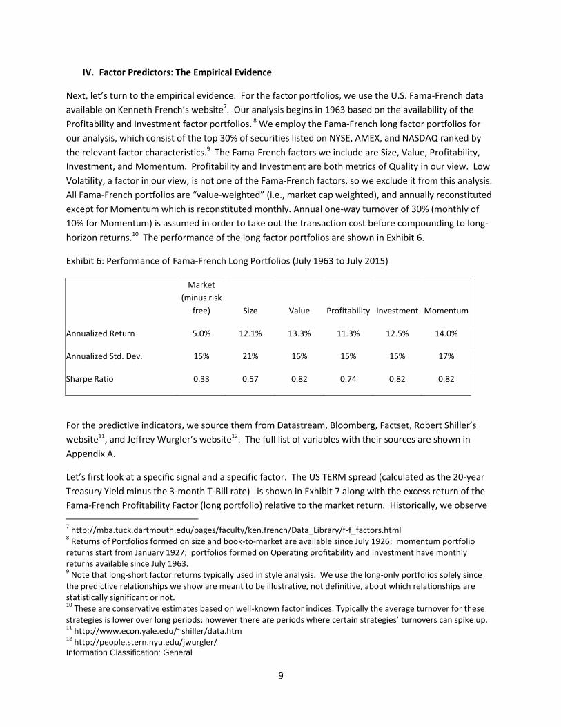
IV. Factor Predictors: The Empirical Evidence

Next, let’s turn to the empirical evidence. For the factor portfolios, we use the U.S. Fama-French data

available on Kenneth French’s website7. Our analysis begins in 1963 based on the availability of the

Profitability and Investment factor portfolios. 8 We employ the Fama-French long factor portfolios for

our analysis, which consist of the top 30% of securities listed on NYSE, AMEX, and NASDAQ ranked by

the relevant factor characteristics.9 The Fama-French factors we include are Size, Value, Profitability,

Investment, and Momentum. Profitability and Investment are both metrics of Quality in our view. Low

Volatility, a factor in our view, is not one of the Fama-French factors, so we exclude it from this analysis.

All Fama-French portfolios are “value-weighted” (i.e., market cap weighted), and annually reconstituted

except for Momentum which is reconstituted monthly. Annual one-way turnover of 30% (monthly of

10% for Momentum) is assumed in order to take out the transaction cost before compounding to long-

horizon returns.10 The performance of the long factor portfolios are shown in Exhibit 6.

Exhibit 6: Performance of Fama-French Long Portfolios (July 1963 to July 2015)

Market

(minus risk

free) Size Value Profitability Investment Momentum

Annualized Return 5.0% 12.1% 13.3% 11.3% 12.5% 14.0%

Annualized Std. Dev. 15% 21% 16% 15% 15% 17%

Sharpe Ratio 0.33 0.57 0.82 0.74 0.82 0.82

For the predictive indicators, we source them from Datastream, Bloomberg, Factset, Robert Shiller’s

website11, and Jeffrey Wurgler’s website12. The full list of variables with their sources are shown in

Appendix A.

Let’s first look at a specific signal and a specific factor. The US TERM spread (calculated as the 20-year

Treasury Yield minus the 3-month T-Bill rate) is shown in Exhibit 7 along with the excess return of the

Fama-French Profitability Factor (long portfolio) relative to the market return. Historically, we observe

7 http://mba.tuck.dartmouth.edu/pages/faculty/ken.french/Data_Library/f-f_factors.html

8 Returns of Portfolios formed on size and book-to-market are available since July 1926; momentum portfolio

returns start from January 1927; portfolios formed on Operating profitability and Investment have monthly returns available since July 1963. 9 Note that long-short factor returns typically used in style analysis. We use the long-only portfolios solely since

the predictive relationships we show are meant to be illustrative, not definitive, about which relationships are statistically significant or not. 10

These are conservative estimates based on well-known factor indices. Typically the average turnover for these strategies is lower over long periods; however there are periods where certain strategies’ turnovers can spike up. 11

http://www.econ.yale.edu/~shiller/data.htm 12

http://people.stern.nyu.edu/jwurgler/


that a steepening of the yield curve (a widening of the TERM spread), coincides with weakening

economic conditions. The yield curve becomes very steep during economic slowdowns, the steepest

point usually occurring at the trough of a recession (which has historically been predictive for future

growth as discussed in Fama and French (1989). During the trough of a recession, investors require

higher compensation for risk-seeking assets, including equities. Defensive assets are likely to

underperform coming out of a recession. Therefore a steep curve has preceded periods of poor

performance to the Profitability Factor portfolio. This agrees with the rationale we proposed earlier—

Profitability is generally defensive, favoring large low growth stable companies.

Exhibit 7: US TERM Spread and the Fama-French Profitability Long Factor Portfolio (July 1963 to July

2015)

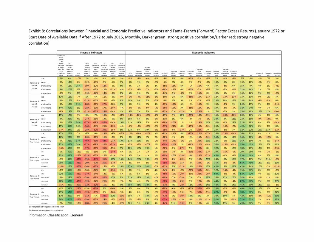
We show correlations next as a way to summarize the relationship between various predictors and

factors in a single metric. Correlations between predictors and future factor returns capture the general

direction between signals and factors, and are indicative of general magnitude, however, they are overly

simple in that they are linear and cannot adequately accommodate the relationship between regimes.

Exhibit 8 summarizes the correlations between a range of economic and financial signals and future

factor returns at different horizons. The correlations between TERM Spread and Profitability are

negative as expected across all horizons. The correlations become increasingly negative as we extend

the horizon. At 1 month, the correlation is only -0.18 but at one year, the correlation is -0.46, a strong

relationship. Past 1 year, the correlation stays steady around -0.29 to -0.35.

-15

-10

-5

0

5

10

15

20

25

-3

-2

-1

0

1

2

3

4

5

19

59

01

19

61

01

19

63

01

19

65

01

19

67

01

19

69

01

19

71

01

19

73

01

19

75

01

19

77

01

19

79

01

19

81

01

19

83

01

19

85

01

19

87

01

19

89

01

19

91

01

19

93

01

19

95

01

19

97

01

19

99

01

20

01

01

20

03

01

20

05

01

20

07

01

20

09

01

20

11

01

20

13

01

20

15

01

Forw

ard

1-y

ear

Exc

ess

Re

turn

%

%

Term spread (LHS) profitability premium for1y (RHS)


11

Exhibits 9, 10, and 11 show the correlations for other signals—Housing Market, Sentiment, Shiller

“Valuation-based” metrics, and Momentum, or past factor returns. In the exhibits, the darkest green

cells are the most positive correlations; the darkest red cells are the most negative correlations. Both

dark green and red green can be used as predictive signals as we would merely reverse the sign if

needed.


Exhibit 8: Correlations Between Financial and Economic Predictive Indicators and Fama-French (Forward) Factor Excess Returns (January 1972 or

Start Date of Available Data if After 1972 to July 2015, Monthly, Darker green: strong positive correlation/Darker red: strong negative

correlation)

Corporate

credit

spread

(Yield

Spread

between

M oody's

BAA and

AAA

Corporate

Bond)

TED

spread (3-

month

InterBank

Rate - 3-

month T-

Bill rate)

TED

spread 2

Term

spread

(Treasury

Yield 20-

year - 3-

month T-

Bill rate)

YoY

growth of

monetary

base

adjusted

after

inf lat ion

YoY

growth of

money

supply M 1

adjusted

after

inf lat ion

YoY

growth of

money

supply M 2

adjusted

after

inf lat ion

YoY

growth of

commercial

bank assets

- Loans and

leases in

bank credit

GDP

growth

Personal

Consumpti

on growth

Private

Domestic

Fixed

investment

growth

Current

account

growth

Unit output

growth

Corporate

prof it

growth

Change in

Bankrupty

f ilings

Changein

capacity

rat io

Change in

total

t reasury

securit ies

Change in

Consumer

Credit

Personal

Savings

Rate

Change in

Consumer

Conf idence

Index

Change in

personal

income CPI PPI

Change in

CPI

Change in

PPI

Unemploym

ent rate

size 7% 6% -10% 2% -4% -6% -2% -5% -6% -5% -6% -1% -5% 2% 4% -10% -5% -6% 7% -4% -6% 7% 6% -1% 0% 3%

value 0% 14% -8% -12% -13% -9% -5% 3% 6% 7% 4% -3% -6% 3% 4% 1% -5% -2% 14% 9% 8% 13% 10% -2% -3% 0%

profitability 4% 11% 25% -19% -12% -18% -5% 6% 3% 2% 0% 2% -15% -13% 6% -1% -10% 6% 10% -6% 6% 15% 9% 4% 1% -7%

investment 9% 20% 1% -18% -13% -12% -12% -4% -5% -4% -7% -2% -19% -11% 0% -10% -7% -5% 12% -3% -4% 21% 16% 2% 0% 4%

momentum -6% 9% 3% -13% -17% -14% -9% 1% 5% 5% 3% 4% -14% -5% -7% 1% -15% 0% 10% 1% 2% 16% 12% 9% 8% -7%

size 12% 11% -7% 1% -6% -11% -5% -9% -9% -9% -11% -5% -10% -2% 6% -18% -10% -11% 12% -13% -13% 13% 11% 0% 0% 3%

value 4% 16% -8% -21% -15% -12% -5% 6% 10% 9% 6% -6% -8% 5% 5% 0% -7% -4% 23% 10% 12% 18% 14% -6% -9% 0%

profitability 3% 18% 31% -28% -21% -27% -10% 9% 6% 5% 0% 3% -23% -18% 5% -2% -15% 9% 15% -8% 9% 24% 15% 7% 4% -11%

investment 14% 30% 6% -28% -20% -17% -18% -4% -6% -6% -9% -7% -28% -15% 3% -15% -12% -8% 19% -6% -5% 32% 24% 4% -1% 6%

momentum -9% 19% 5% -21% -27% -24% -14% 4% 8% 7% 7% 0% -22% -7% -12% 1% -23% 1% 17% -2% 3% 25% 19% 12% 12% -10%

size 15% 17% -7% 0% -7% -15% -7% -11% -13% -12% -14% -7% -17% -7% 10% -23% -14% -15% 16% -24% -18% 20% 16% 4% 2% 4%

value 8% 21% 4% -24% -15% -13% -5% 6% 10% 8% 6% -5% -11% 3% 6% -2% -7% -9% 28% 8% 13% 23% 18% -9% -12% 0%

profitability 3% 27% 34% -37% -29% -36% -14% 13% 11% 11% 2% -1% -29% -20% 1% -1% -19% 14% 20% -6% 13% 31% 19% 6% 3% -14%

investment 19% 35% 14% -36% -24% -21% -22% -4% -7% -8% -10% -6% -37% -21% 4% -19% -16% -10% 25% -14% -7% 42% 32% 6% 2% 8%

momentum -14% 24% 0% -28% -32% -29% -15% 6% 12% 9% 10% -6% -29% -8% -17% 2% -28% 3% 23% -5% 3% 32% 22% 16% 13% -12%

size 15% 27% -7% -2% -9% -19% -8% -12% -10% -10% -14% 3% -21% -11% 8% -25% -22% -17% 23% -23% -16% 26% 21% 6% -1% 2%

value 16% 28% 9% -20% -21% -16% -8% 1% 9% 11% 3% 2% -22% -1% -2% -2% -11% -16% 36% 8% 11% 34% 28% -8% -10% 3%

profitability 0% 32% 37% -46% -33% -44% -21% 17% 17% 16% 8% -2% -34% -17% -9% 1% -20% 19% 22% -3% 16% 35% 19% 7% 5% -14%

investment 25% 47% 24% -37% -28% -27% -31% -6% -7% -7% -10% 2% -50% -24% 2% -16% -22% -10% 30% -15% -10% 55% 43% 12% 7% 11%

momentum -16% 30% 0% -37% -28% -31% -15% 9% 22% 15% 19% 1% -32% -2% -27% 5% -29% 8% 32% 0% 10% 38% 21% 12% 2% -13%

size 5% 30% -12% -7% -16% -1% -34% -6% 5% 2% -2% 1% -20% -7% 3% -20% -30% -12% 29% -16% -6% 29% 26% 4% -7% -5%

value 23% 45% -22% -31% -22% -12% -11% -7% 3% 5% -1% 2% -40% -10% -19% -8% -23% -22% 48% -4% -3% 53% 46% 4% 2% 8%

prof itability -3% 31% -43% -35% -43% -31% 16% 16% 24% 20% 19% -4% -37% -8% -20% 5% -16% 23% 24% 8% 15% 37% 17% 9% 11% -8%

investment 25% 59% -38% -29% -27% -30% -17% -6% 2% 0% 1% -4% -59% -21% -15% -4% -23% -6% 35% -6% -8% 64% 49% 13% 8% 13%

momentum -18% 27% -36% -26% -33% -15% -6% 14% 37% 24% 34% -5% -32% 8% -21% 11% -26% 15% 42% 8% 22% 42% 24% 10% -2% -12%

size -1% 31% -19% -16% -24% 1% -23% -2% 8% 7% 2% 4% -24% -8% -9% -20% -36% -10% 32% -14% -4% 35% 37% 8% 3% -3%

value 22% 55% -32% -37% -24% -12% -9% -5% 5% 8% 1% 1% -46% -15% -29% -11% -28% -20% 60% -5% -4% 62% 52% 4% 5% 12%

prof itability 4% 28% -31% -29% -28% -32% 10% 9% 21% 17% 23% -4% -40% -7% -23% 7% -7% 23% 26% 17% 15% 34% 10% -1% -1% 4%

investment 28% 60% -40% -32% -22% -21% -7% -7% 7% 4% 8% -3% -58% -18% -23% 1% -17% -6% 44% 3% -4% 67% 50% 7% 6% 23%

momentum -15% 22% -26% -32% -32% -15% -4% 6% 30% 21% 32% 0% -37% 7% -28% 11% -23% 14% 43% 9% 14% 45% 30% 13% 5% -1%

size -1% 33% -27% -15% -32% 2% -16% -3% 5% 0% 6% 3% -29% -6% -9% -15% -37% -7% 35% -7% -5% 40% 44% 11% 1% 3%

value 25% 62% -35% -32% -29% -8% -16% -9% 4% 0% 8% -3% -57% -15% -13% -7% -33% -15% 67% -8% -3% 70% 57% 8% 3% 22%

prof itability 17% 29% -9% -31% -5% -38% 12% -18% 10% 3% 18% -2% -47% 2% -30% 14% 8% 3% 30% 19% 1% 42% 18% -8% -10% 39%

investment 36% 60% -29% -29% -23% -24% -9% -19% 0% -5% 8% -2% -65% -16% -13% -4% -11% -11% 51% 0% -10% 71% 53% 1% -4% 42%

momentum 2% 26% -13% -28% -20% -21% -4% -13% 16% 9% 23% 3% -44% 11% -33% 8% -10% 4% 51% 15% 5% 49% 37% 1% -7% 27%

Darker green: strong positive correlation

Darker red: strong negative correlation

Financial Indicators Economic Indicators

Forward 5

Year return

Forward 1

Month

return

Forward 3

Month

return

Forward 6

Month

return

Forward 1

Year return

Forward 2

Year return

Forward 3

Year return


13

Exhibit 9: Correlations Between Housing, Sentiment, and Shiller “Valuation” Predictive Indicators and Fama-French (Forward) Factor Excess

Returns (January 1972 or Start Date of Available Data if After 1972 to July 2015, Monthly, Darker green: strong positive correlation/Darker red:

strong negative correlation)


Sales of

new homes

Sales of

exist ing

homes

Home

builder

Unit

housing

started VIX average SENT^ SENT DSENT^ DSENT

Leading

indicator ISM PM I CAPE Div Yield Earn yield

size 6% -1% 1% 3% -3% -9% -10% 4% 6% -7% -3% -4% 9% 8%

value 4% 1% 4% 1% -18% 2% 0% 6% -4% 1% 4% -8% 11% 11%

profitability -8% -11% -20% -5% 5% 13% 13% -4% -1% -6% -5% -8% 15% 13%

investment -1% -5% 0% -3% -4% 7% 3% 6% -2% -11% -5% -14% 18% 18%

momentum 0% -8% 2% -1% -17% -4% -5% 5% 5% 1% -6% -6% 13% 17%

size 3% -6% -3% 2% 5% -14% -17% 2% 4% -14% -11% -7% 16% 14%

value 6% 1% 4% 2% -19% 1% -2% 8% -1% 1% 5% -13% 18% 16%

profitability -12% -17% -31% -9% -1% 20% 19% -7% -3% -6% -8% -13% 24% 23%

investment -4% -9% 0% -5% -8% 10% 4% 5% 3% -17% -9% -20% 28% 28%

momentum -3% -14% 3% -4% -24% -6% -6% 1% 5% 2% -11% -10% 23% 29%

size -2% -10% -7% -2% 15% -21% -23% 0% 0% -19% -18% -12% 24% 20%

value 5% -1% -3% 2% -10% 0% -5% 6% 0% 1% 5% -17% 24% 20%

profitability -16% -20% -38% -10% -12% 26% 24% -7% -7% -5% -9% -17% 32% 33%

investment -5% -13% -4% -6% -5% 13% 6% 6% 6% -21% -14% -27% 37% 37%

momentum -8% -16% 1% -7% -32% -10% -9% 0% -3% 3% -16% -15% 31% 39%

size -8% -19% 0% -9% 25% -26% -29% 6% 7% -21% -21% -13% 30% 26%

value 7% -3% -4% 4% -10% -4% -10% 7% 7% 1% 8% -22% 33% 29%

profitability -17% -23% -44% -12% -21% 26% 25% -4% -3% -1% -10% -22% 41% 43%

investment -8% -21% -10% -9% 0% 14% 6% 5% 6% -21% -16% -34% 49% 51%

momentum -9% -16% 0% -9% -30% -15% -13% 3% -2% 6% -15% -22% 42% 49%

size -18% -16% -6% -17% 38% -44% -46% 5% 9% -16% -13% -11% 30% 28%

value -5% -14% -6% -3% -10% -18% -26% 8% 10% -7% 0% -32% 48% 46%

prof itability -4% -17% -33% 1% -38% 24% 24% 1% -1% 10% -6% -32% 52% 53%

investment -19% -28% -16% -14% -8% 6% 0% 3% 2% -16% -11% -42% 60% 64%

momentum -2% -2% -2% -2% -29% -31% -30% 2% 3% 15% -3% -33% 53% 55%

size -12% -14% -8% -13% 36% -52% -57% 6% 10% -11% -10% -10% 29% 32%

value -1% -11% 7% 2% -3% -20% -29% 7% 7% -5% -2% -42% 59% 59%

prof itability 1% -11% -11% 6% -47% 23% 23% -1% -1% 13% -9% -41% 59% 57%

investment -9% -17% 8% 0% -11% -3% -9% 3% 3% -7% -7% -49% 67% 72%

momentum 6% 3% 7% 5% -33% -39% -39% 4% 4% 16% -6% -40% 57% 60%

size -10% -7% -2% -10% 46% -56% -61% 5% 6% -13% -7% -13% 27% 36%

value -4% -15% 17% 2% 14% -14% -23% 4% 4% -10% -5% -51% 68% 70%

prof itability 4% -13% 14% 12% -56% 6% 7% 4% 5% 16% -3% -57% 69% 68%

investment -4% -15% 27% 1% -7% -11% -18% 4% 5% -11% -9% -61% 78% 82%

momentum 7% 3% 17% 8% -37% -46% -47% 4% 4% 11% -3% -54% 63% 66%



Forward 2

Year return

Forward 3

Year return

Forward 5

Year return

Housing Market Sentiment Shiller Valuation

Forward 1

Month

return

Forward 3

Month

return

Forward 6

Month

return

Forward 1

Year return


15

Exhibit 10: Correlations Between Past Factor Returns (Momentum) and Fama-French (Forward) Factor Excess Returns – Up to 1 Year (January

1972 or Start Date of Available Data if After 1972 to July 2015, Monthly, Darker green: strong positive correlation/Darker red: strong negative

correlation)


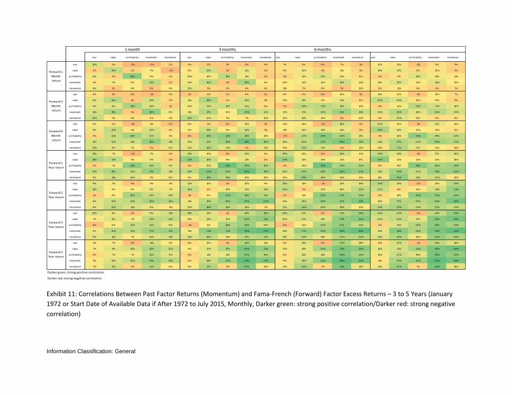
Exhibit 11: Correlations Between Past Factor Returns (Momentum) and Fama-French (Forward) Factor Excess Returns – 3 to 5 Years (January

1972 or Start Date of Available Data if After 1972 to July 2015, Monthly, Darker green: strong positive correlation/Darker red: strong negative

correlation)

size value prof itability investment momentum size value prof itability investment momentum size value prof itability investment momentum size value prof itability investment momentum

size 10% 3% -2% -2% 2% 4% 2% 1% 0% 4% 7% 6% 0% 7% 1% 12% 10% -1% 9% 5%

value 2% 13% 2% 7% -2% 8% 14% 1% 11% 3% 8% 13% 5% 11% 5% 16% 17% 6% 10% 3%

prof itability 8% 3% 19% 6% 4% 10% 10% 16% 11% 2% 5% 13% 17% 13% 6% 4% 9% 19% 15% 11%

investment 5% 7% 6% 13% 2% 10% 16% 1% 19% 8% 10% 12% 12% 19% 13% 15% 19% 12% 19% 13%

momentum 8% 1% 6% 0% 6% 12% 5% 4% 4% 6% 11% 7% 8% 1% 10% 8% 11% 9% 4% 7%

size 4% 1% 0% -1% 3% 1% 4% 2% 4% 1% 8% 6% 0% 10% 1% 14% 12% -1% 12% 7%

value 9% 14% 1% 10% 3% 11% 18% 4% 14% 5% 10% 15% 9% 14% 6% 24% 20% 10% 13% 5%

prof itability 9% 9% 16% 10% 1% 10% 14% 15% 14% 6% 2% 20% 21% 19% 10% 5% 14% 25% 21% 18%

investment 11% 15% 1% 18% 8% 11% 17% 10% 20% 14% 13% 17% 20% 25% 19% 20% 26% 18% 26% 20%

momentum 12% 5% 4% 4% 5% 16% 12% 8% 7% 10% 12% 15% 13% 3% 12% 9% 20% 15% 8% 9%

size 6% 4% -1% 5% 0% 8% 5% 0% 10% 1% 12% 10% -2% 18% 4% 20% 14% -1% 17% 12%

value 8% 12% 5% 10% 4% 9% 15% 9% 14% 5% 11% 14% 14% 14% 5% 28% 16% 13% 12% 9%

prof itability 3% 12% 16% 12% 5% 0% 19% 21% 18% 10% -2% 20% 29% 24% 15% 5% 16% 33% 25% 24%

investment 11% 12% 11% 18% 11% 12% 17% 19% 25% 19% 16% 20% 27% 30% 23% 21% 27% 24% 30% 27%

momentum 10% 9% 7% 2% 9% 12% 16% 12% 3% 12% 10% 20% 17% 5% 13% 10% 27% 17% 13% 10%

size 11% 7% -2% 7% 3% 14% 10% 0% 13% 6% 19% 13% 0% 19% 12% 24% 18% -1% 17% 19%

value 15% 13% 5% 8% 2% 21% 16% 9% 11% 4% 26% 14% 13% 12% 8% 34% 12% 12% 14% 16%

prof itability 2% 7% 19% 14% 9% 3% 12% 25% 20% 16% 4% 14% 32% 24% 22% 8% 15% 35% 28% 30%

investment 13% 15% 13% 17% 11% 16% 22% 20% 26% 19% 18% 24% 25% 30% 27% 21% 29% 23% 31% 32%

momentum 8% 11% 10% 5% 8% 9% 19% 16% 10% 10% 10% 25% 19% 14% 10% 15% 33% 21% 22% 10%

size 9% 7% 0% 5% 5% 12% 10% 1% 10% 9% 19% 13% -1% 14% 16% 26% 18% -2% 16% 26%

value 11% 6% 6% 8% 7% 16% 6% 10% 12% 14% 20% 4% 13% 15% 20% 23% 8% 14% 21% 31%

prof itability 1% 6% 16% 12% 10% 1% 8% 22% 19% 17% 2% 11% 28% 27% 24% 6% 15% 33% 33% 32%

investment 9% 12% 13% 16% 14% 11% 16% 20% 23% 23% 14% 19% 26% 27% 31% 16% 27% 27% 30% 38%

momentum 9% 13% 11% 8% 5% 12% 19% 16% 14% 7% 17% 24% 20% 19% 12% 25% 29% 23% 27% 23%

size 10% 8% 0% 9% 11% 15% 13% 1% 16% 19% 19% 17% 0% 21% 25% 24% 24% -3% 25% 33%

value 7% 9% 7% 13% 13% 10% 13% 12% 20% 21% 16% 17% 15% 27% 30% 20% 24% 17% 35% 39%

prof itability 0% 6% 12% 13% 8% -1% 9% 18% 20% 14% 0% 12% 23% 27% 20% 5% 19% 26% 35% 29%

investment 8% 14% 13% 17% 17% 11% 21% 21% 26% 27% 15% 27% 26% 33% 35% 18% 35% 28% 39% 42%

momentum 9% 11% 7% 10% 11% 13% 16% 11% 17% 17% 15% 20% 15% 22% 22% 19% 28% 16% 32% 28%

size 5% 7% 0% 11% 6% 6% 10% 1% 18% 11% 9% 15% 0% 23% 15% 10% 20% -1% 25% 19%

value 7% 9% 10% 15% 12% 9% 12% 17% 24% 21% 13% 15% 24% 31% 29% 18% 21% 29% 38% 40%

prof itability 3% 7% 7% 13% 9% 4% 11% 11% 22% 16% 8% 15% 15% 30% 24% 16% 22% 19% 38% 32%

investment 5% 10% 12% 17% 14% 6% 15% 20% 27% 23% 9% 19% 28% 36% 32% 11% 29% 32% 43% 39%

momentum 7% 11% 3% 14% 6% 9% 17% 5% 23% 10% 13% 24% 7% 31% 15% 16% 32% 7% 38% 18%



Forward 5

Year return

Forward 1

Month

return

Forward 3

Month

return

Forward 6

Month

return

Forward 1

Year return

Forward 2

Year return

Forward 3

Year return

1 month 3 months 6 months


17

size value prof itability investment momentum size value prof itability investment momentum size value prof itability investment momentum

size 11% 9% -2% 6% 6% 11% 8% -1% 7% 11% 4% 4% 1% 5% 7%

value 14% 10% 7% 9% 10% 10% 10% 6% 8% 13% 8% 9% 6% 8% 12%

prof itability 5% 10% 17% 16% 17% 5% 12% 15% 16% 16% 15% 21% 14% 19% 22%

investment 12% 15% 11% 15% 17% 12% 17% 11% 14% 19% 12% 16% 14% 16% 21%

momentum 11% 14% 9% 8% 7% 12% 13% 7% 10% 13% 13% 17% 7% 13% 12%

size 14% 12% -3% 9% 9% 16% 11% -2% 10% 17% 3% 5% -1% 7% 9%

value 20% 11% 10% 11% 17% 14% 14% 9% 12% 21% 12% 11% 8% 11% 18%

prof itability 7% 15% 23% 23% 24% 8% 19% 20% 24% 24% 22% 31% 20% 29% 34%

investment 16% 21% 16% 21% 26% 17% 25% 16% 20% 29% 16% 23% 20% 23% 32%

momentum 15% 24% 15% 14% 10% 20% 22% 12% 17% 22% 17% 28% 11% 22% 18%

size 19% 15% -5% 12% 16% 21% 16% -5% 14% 25% 3% 6% -2% 9% 12%

value 21% 9% 12% 12% 22% 18% 16% 10% 15% 29% 13% 12% 11% 14% 23%

prof itability 8% 19% 30% 32% 33% 10% 24% 25% 31% 32% 30% 40% 25% 38% 44%

investment 18% 24% 20% 24% 32% 22% 31% 20% 25% 37% 18% 28% 25% 28% 39%

momentum 19% 30% 18% 19% 16% 23% 29% 16% 23% 29% 19% 36% 11% 28% 22%

size 25% 19% -4% 14% 27% 24% 19% -6% 16% 32% 1% 7% -2% 10% 14%

value 21% 9% 12% 16% 32% 20% 18% 11% 20% 37% 15% 14% 15% 19% 32%

prof itability 12% 20% 35% 37% 40% 15% 31% 28% 39% 41% 38% 49% 30% 47% 54%

investment 17% 28% 22% 26% 39% 23% 35% 22% 31% 45% 19% 34% 27% 33% 46%

momentum 27% 34% 24% 28% 28% 26% 34% 20% 34% 36% 23% 42% 12% 35% 25%

size 27% 23% -6% 19% 36% 20% 21% -8% 19% 30% 0% 6% -7% 7% 12%

value 17% 18% 14% 29% 47% 17% 23% 18% 31% 46% 22% 21% 22% 29% 41%

prof itability 11% 25% 31% 42% 41% 22% 41% 28% 48% 48% 39% 55% 32% 56% 58%

investment 19% 35% 27% 34% 49% 24% 39% 33% 42% 55% 24% 42% 32% 41% 50%

momentum 30% 33% 22% 38% 40% 32% 44% 18% 48% 39% 21% 45% 8% 41% 25%

size 21% 27% -5% 26% 34% 13% 24% -5% 25% 28% -7% 4% -9% 4% 5%

value 17% 28% 24% 41% 50% 18% 32% 26% 43% 51% 26% 28% 20% 35% 42%

prof itability 16% 33% 27% 45% 41% 29% 49% 25% 54% 51% 42% 60% 30% 58% 60%

investment 20% 39% 36% 46% 53% 22% 46% 40% 54% 60% 25% 49% 34% 50% 52%

momentum 27% 40% 16% 47% 35% 28% 49% 10% 53% 34% 13% 47% 4% 40% 22%

size 5% 18% -6% 21% 19% -5% 10% -9% 11% 8% -22% -7% -15% -11% -13%

value 19% 26% 33% 44% 49% 21% 29% 28% 44% 49% 27% 31% 11% 31% 41%

prof itability 26% 37% 21% 52% 45% 33% 53% 22% 60% 54% 37% 60% 23% 62% 56%

investment 14% 37% 34% 51% 46% 18% 45% 34% 56% 50% 23% 48% 20% 47% 45%

momentum 18% 40% 2% 47% 22% 14% 48% 1% 47% 20% -4% 36% -1% 26% 7%



Forward 3

Month

return

Forward 1

Year return

Forward 3

Year return

Forward 5

Year return

Forward 2

Year return

Forward 6

Month

return

Forward 1

Month

return


The correlations suggest some predictive information in a subset of the signals. For instance, the TED

Spread and TERM Spread (Financial Conditions indicators) are reasonably strong predictors for horizons

greater than 6 months, particularly for Value, Profitability, Investment, and Momentum. Within the

Economic Conditions category, four signals – Unit Output growth, Personal Savings rate, CPI, and PPI

have reasonably strong correlations with Value and Investment factors at horizons of one year and

higher. The VIX and Sentiment metrics have strong predictive relationships at 1 year horizons and up

but the impact is not uniform across all factors. The valuation metrics have strong relationship with

future factor performance, particularly at longer horizons. Past factor returns as a signal appears

significant for some factors as early as 3 months out (and strongest for Size, Value, Profitability, and

Investment), but at 1 year+ horizons, the impact is strongest across all factors, though at 3 and 5 year

horizons, some evidence of mean reversion starts to appear.

In sum, there do appear to be a few relationships that corroborate the theory, particularly the positive

relationship between valuation and future factor returns, the positive relationship between past

performance (momentum/persistence) and future factor returns, the positive relationship between

Sentiment and Size/Value, and the negative relationship between Sentiment and

Profitability/Investment. Certainly the horizon matters and few signals appear to be strong at very short

1-month horizons.

V. The Perils and Pitfalls of Factor Timing

There is however a long leap between the sometimes significant correlations we have observed

historically and the successful application of a factor timing model. Moreover, we should be concerned

that randomness alone may explain some of the historical relationships we observe. Certainly some

signals have shown efficacy just by luck. In this section, we look at the practical challenges of building a

model and identify the major pitfalls.

We identify three main challenges to building a factor timing model:

Time-Varying Relationships

Cherry-Picking of Indicators Based on Perfect Hindsight

Data Revisions

We next discuss each one of these in turn.

Time varying relationships

The most important challenge we see is the problem of time-varying relationships between indicators

and factors. As an example, we plot the US Corporate Credit Spread, measured as the Yield Spread

between BAA and AAA Corporate Bonds in Exhibit 12 (Source: Barclays). Widening credit spreads

preceded a period of good performance for Value in 2000-2001 but a period of poor performance in

2008-2009.

What was different about these two periods? We suspect that the most important difference was that

Value was low beta in 2000-2001 coming off the heels of the Tech Bubble when Growth stocks were


19

high beta, but Value was high beta in 2008-2009 (see Exhibit 11). There were of course other

differences between the economic and financial conditions in these two periods. In 2000-2001,

economic growth remained stronger for the US’ major trading partners while in 2008-2009, the GFC had

a widespread impact on economies around the world. However, we suspect that the differences were

more to do with the changing nature of Value than differences in the underlying conditions which

corporate credit spreads were tied to.

Exhibit 12: US Corporate Credit Spread and the Fama-French Value Long Factor Portfolio (July 1963 to

July 2015)

Exhibit 13: Beta of Value Factor to Market

-30

-20

-10

0

10

20

30

40

50

60

0

0.5

1

1.5

2

2.5

3

3.5

4

19

59

01

19

61

01

19

63

01

19

65

01

19

67

01

19

69

01

19

71

01

19

73

01

19

75

01

19

77

01

19

79

01

19

81

01

19

83

01

19

85

01

19

87

01

19

89

01

19

91

01

19

93

01

19

95

01

19

97

01

19

99

01

20

01

01

20

03

01

20

05

01

20

07

01

20

09

01

20

11

01

20

13

01

20

15

01

Forw

ard

1-y

ear

Exc

ess

Re

turn

%

%

corporate credit spread (LHS) value premium for1y (RHS)

-0.8

-0.6

-0.4

-0.2

0

0.2

0.4

19

66

07

19

68

07

19

70

07

19

72

07

19

74

07

19

76

07

19

78

07

19

80

07

19

82

07

19

84

07

19

86

07

19

88

07

19

90

07

19

92

07

19

94

07

19

96

07

19

98

07

20

00

07

20

02

07

20

04

07

20

06

07

20

08

07

20

10

07

20

12

07

20

14

07B

eta

of

the

Fam

a-F

ren

ch V

alu

e F

acto

r to

th

e M

arke

t


The implications for a factor timing model are clear—the model must take into account the dynamic

nature of factors.

Cherry-Picking of Indicators Based on Perfect Hindsight

The second significant challenge in factor timing is the age-old problem of 20/20 hindsight and data

mining. Being able to identify signals that have worked well at predicting factors historically is not the

same as picking signals today that will work well at predicting factors in the future. Even grounding

models as much as possible in strong theory and academic backing is not sufficient as academic research

tends to cluster around signals that appear predictive; those that do not usually do not receive a lot of

attention.

As an example of the dangers of “cherry-picking” signals, we conduct a simple exercise. We imagine

putting ourselves in the year 1990 and asking which predictor/factor relationships we would have

observed between 1970 and 1990. We then fast forward and see whether these predictive signals

would have worked between 1990 and 2010.

The results are summarized in Exhibit 14. Not unexpectedly, we find that many of the factors that were

strong in 1970-1990 were not especially strong in 1990-2010. Specifically, we run univariate regressions

of non-overlapped 3-month factor excess returns against the 38 macro variables13 using data available in

1990. There we find 19 predictors which have statistically significant beta coefficients for size, 5 for

value, 2 for profitability, 10 for investment and 10 for momentum. However when we repeat the same

set of univariate regressions using data from 1990 to 2010, only 1 is still significant for size, 2 for

profitability, 2 for momentum, and none for value and investment. This pattern does not change much

with the return horizon.

13

The 38 factors are: Corporate credit spread, TED spread, Term spread, M base, M1, M2, DJIA, Bank loans, GDP, personal consumption, private fixed investment, Current Account, Unit output, Corporate profit, Capacity ratio, Total treasury outstanding, Total consumer credit, Savings rate, Consumer Confidence Index, Personal income, CPI, PPI, Change in CPI, Change in PPI, unemployment rate, Unemploy initial claims 4-wk avg, Sales of new homes, Sales of existing homes, Unit housing started, SENT^, SENT, DSENT^, DSENT, Leading indicator, ISM PMI, CAPE, Div Yield, Earnings yield. For exact details on the measures, please see Appendix A.


21

Exhibit 14: Number of Statistically Significant in the First Sub-period and in Both Subperiods

3-Month Horizon Mkt-RF size value profitability investment momentum

Number of predictors statistically significant in 1972 – 1989 5 18 3 2 10 9 Number of predictors are confirmed statistically significant in the same direction in 1990 - 2010 0 1 0 2 0 1


Number of predictors statistically significant in 1972 – 1989 1 17 3 3 6 14 Number of predictors are confirmed statistically significant in the same direction in 1990 - 2010 0 1 0 2 0 0


Number of predictors statistically significant in 1972 - 1989 3 14 5 4 14 13 Number of predictors are confirmed statistically significant in the same direction in 1990 - 2010 1 1 0 2 1 1

Note: For the horizon shown, returns for that horizon are regressed at that Frequency. For example, if the horizon is 3 months, we use 3 month

returns and regress these returns on the predictors quarterly.


Data Revisions

The third major challenge concerns data revisions, particularly for macroeconomic indicators. Most

macroeconomic data series are revised. Although financial data, such as bilateral exchange rates and

security prices, generally are not revised, measures of real economic activity and aggregate prices

typically are. GDP and the unemployment rate are two headline macroeconomic indicators that are

often restated after the initial estimate has been reported. Therefore, backtests that include these

indicators may not accurately reflect the information that would have been available at the time of the

forecast.

VI. Overcoming the Challenges to Timing Factors

As we have seen, factor timing is sufficiently challenging that one should be appropriately skeptical of the range of marketed timing models available. We share many of the misgivings around the challenges of factor timing highlighted in Asness (2016). We do not, however, believe the endeavor is completely futile. In particular, factor timing can have its rightful place in a manager’s toolkit if an investor has a sufficiently long horizon and understands that even a good factor timing strategy will not be successful in every period.

There are a few potential approaches worth discussing. The first is to use a parsimonious model. The

objective is to use only a few indicators that are well vetted and have theoretical intuition. We

recognize upfront that this approach will not utilize the full available information set but is less

susceptible to noise and cherry-picking. Valuation and Trend signals are good candidates in this vein.

Consider an example using only Valuation as a signal, based on the Campbell and Schiller (1998)

framework, in which one avoids factors when they are unusually expensive. This framework was

originally proposed in Shapiro and Thomas (2014) and more recently extended by Arnott, Beck, and

Kalesnik (2017). The portfolio is equally weighted across four factor portfolios: Value, Size, Low

Volatility, and Quality. Once a month, stocks are sorted based on the underlying Value, Size, Low

Volatility, and Quality metrics and divided into quintiles. The spread in B/P is calculated as the median

B/P of the top quintile minus the median B/P of the bottom quintile. When this spread is large and

positive, the factor is attractively priced (cheap). When the spread is negative, the factor is expensive.

The current spread is compared against an average of the historical spread. If the former flags a given

factor as expensive and it is more than 1 standard deviation outside the historical spread, that factor is

removed from the portfolio for 3 years. The remaining factors are equal-weighted. (The factor

portfolios used are all based on the MSCI World universe.) The results of this dynamic strategy are

compared against the equal weighted static version in Exhibit 15. Over a 20 year period ending in May

2014, the timed dynamic portfolio exhibited 11.28% annualized returns versus 9.14% for the static

portfolio and 7.57% for the MSCI World Index.


23

Exhibit 15: An Illustration of a Timing Strategy with Factor Valuation (January 1993 to May 2014, USD

Gross Returns)

Note: Index returns reflect capital gains and losses, income and the reinvestment dividends.

At the other end of the spectrum, a more fully fledged multi-signal model which integrates a wide range

of indicators, and accounts for how they interact, is also a compelling candidate framework, particularly

for horizons less than a year. The benefit of this approach is that it can make use of more nuanced

relationships between signals and factors.

Consider an example where four predictive themes are used – Valuation, Persistence (Momentum), an

indicator reflecting the Macroeconomic Cycle phase, and Risk Sentiment, reflecting investors’ risk

appetite. As shown in Exhibit 16, a model built using these indicators is applied to four factor portfolios:

Value, Momentum, Low Volatility, and Quality. The model accounts for the interdependencies of

macroeconomic and market behavioral influences on factor premia by employing a structured

multivariate panel regression framework. Exhibit 16 illustrates the hypothetical value added by this

factor timing model to a static, equally weighted allocation to the four factor portfolios. The dynamic

portfolio outperformed the static portfolio by 1.08% on an annualized basis over the 18-year period

January 1997 to September 2015, while the tracking error versus the MSCI World index decreased by

0.05% , resulting in an improvement in the information ratio from 0.88 to 1.17.

0

2

4

6

8

10

12

1/1

/19

93

11

/1/1

99

3

9/1

/19

94

7/1

/19

95

5/1

/19

96

3/1

/19

97

1/1

/19

98

11

/1/1

99

8

9/1

/19

99

7/1

/20

00

5/1

/20

01

3/1

/20

02

1/1

/20

03

11

/1/2

00

3

9/1

/20

04

7/1

/20

05

5/1

/20

06

3/1

/20

07

1/1

/20

08

11

/1/2

00

8

9/1

/20

09

7/1

/20

10

5/1

/20

11

3/1

/20

12

1/1

/20

13

11

/1/2

01

3

MSCI World Index Static Weights Dynamic Weights


Exhibit 16: An Illustration of a Timing Strategy with Multiple Predictors Embedding Sentiment and

Macroeconomic Variables (January 1997 to September 2015, USD Gross Returns)

VII. Conclusion

Depending on whom you ask, factor timing is a topic that elicits a spectrum of reactions, ranging

from utter futility to unbridled enthusiasm.14 Although the task of forecasting factor premia is

clearly far from trivial, we believe that forecasting fluctuations of factor payoffs can have its place in

the suite of investment insights. Aside from increasing effective breadth by adding another

dimension to an investor’s views, we believe it can play a role in helping position portfolios to better

reflect the evolving environment.

There are ways to build robust timing models, keeping in mind that these models should be tailored

to the horizon. For reasonably long investment horizons, even parsimonious approaches may be

fruitful. We document that some predictors appear to have been reasonably effective at predicting

factors historically over certain horizons. At the same time, cherry-picking relationships in hindsight

poses a real challenge. We show that only a small subset of predictor-factor relationships chosen in

1990 using past performance would have worked in the subsequent twenty years. The promises of

factor investing are undeniable but the perils are real.

14

This spectrum of emotions has swung considerably over time. Prior to the Global Financial Crisis, the typical active manager would have been in the “don’t bother” camp given the robustness of all-weather static models. In the years after the crisis, factor timing became a “must have”.

0.0

0.5

1.0

1.5

2.0

2.5

3.0

3.5

4.01

99

70

1

19

97

09

19

98

05

19

99

01

19

99

09

20

00

05

20

01

01

20

01

09

20

02

05

20

03

01

20

03

09

20

04

05

20

05

01

20

05

09

20

06

05

20

07

01

20

07

09

20

08

05

20

09

01

20

09

09

20

10

05

20

11

01

20

11

09

20

12

05

20

13

01

20

13

09

20

14

05

20

15

01

20

15

09

Cu

mu

lati

ve N

et A

ctiv

e R

etu

rn

Static Weights Dynamic Weights


25

The intriguing question remains -- what drives the temporality of factor premia? We suspect it is

has a lot to do with the changing mix of long term and short term investors at the margin. Insofar as

the risk tolerance and/or ability of long horizon investors to diversify away short term single and

multifactor return volatility is greater, they provide the natural counterparty to short term investors

who eschew said risks due to reduce ability to diversify and/or inability to patiently weather the

fluctuations. Shifts in that long to short term balance of clienteles will also affect, on margin, the

pricing of a given premium ex post. Parsing out the implications of holding horizon on the nature of

risk and alpha is a topic beyond the scope of this work but is an area we think is fruitful for further

research.


Appendix A: Variables, Definitions, and Sources

Financial Conditions Definition sources From Till

corporate credit spread Yield Spread between Moody's BAA and AAA Corporate Bond Bloomberg 196001 201507

TED spread 1 3-month InterBank Rate - 3-month T-Bill rate Datastream 197201 201507

TED spread 2 3-month InterBank Rate - 3-month T-Bill rate FactSet 198601 201507

Term spread Treasury Yield 20-year - 3-month T-Bill rate Datastream 197201 201507

M base YoY growth of monetary base adjusted after inflation Datastream 196001 201507

M1 YoY growth of money supply M1 adjusted after inflation Datastream 196001 201507

M2 YoY growth of money supply M2 adjusted after inflation Datastream 196001 201507

DJIA YoY growth of Dow Jones Industrial Average Index Datastream 196001 201507

bank loan YoY growth of commercial bank assets - loans and leases in bank credit Datastream 196001 201507

Economy Conditions Definition sources From Till

gdp YoY growth of US gdp (constant price) Datastream 196002 201507

personal consumption YoY growth of personal consumption (constant price) Datastream 196002 201507

private fixed inv YoY growth of domestic private fixed investment (constant price) Datastream 196002 201507

Current Account YoY growth of current account adjusted after inflation Datastream 196102 201507

Unit output YoY growth of output per hour (nonfarm business) adjusted after inflation Datastream 196002 201507

Corporate profit YoY growth of corporate profits adjusted after inflation Datastream 196002 201507

bankcruptcy YoY growth of bankruptcy filings Datastream 198111 201507


27

capacity ratio YoY growth of capacity utilization rate all industry Datastream 196801 201507

tot treasury out YoY growth of totoal treasury securities outstanding adjusted after inflation Datastream 196001 201507

tot cons credit YoY growth of consumer credit outstanding adjusted after inflation Datastream 196001 201507

savings rate personal savings as % of disposable personal income Datastream 195901 201507

Consumer Conf Index YoY growth of consumer confidence index Datastream 196802 201507

personal income YoY growth of personal income adjusted after inflation Datastream 196001 201507

CPI CPI- ALL URBAN SAMPLE: ALL ITEMS - ANNUAL INFLATION RATE NADJ Datastream 195901 201507

PPI US PPI - FINISHED GOODS SADJ Datastream 196001 201507

Change in CPI YoY change of CPI Datastream 196001 201507

change in PPI YoY change of PPI Datastream 196101 201507

unemployment rate unemployment rate Datastream 195901 201507

Unemploy initial claims 4-wk avg YoY growth of smoothed 4-week average of unemployment intial claims Datastream 196801 201507

Housing Market Definition sources From Till

sales of new homes YoY growth of sales of new one family houses adjusted after inflation Datastream 196901 201507

sales of existing homes YoY growth of existing home sales: single-family and condo adjusted after inflation Datastream 198601 201507

home builder YoY growth of national association of home builders index adjusted after inflation Datastream 196001 201507

Unit housing started YoY growth of new private housing units started Datastream


Sentiment Definition sources From Till

VIX average monthly average of high and low VIX FactSet 199001 201507

SENT^

linear combination of first principal component of six sentiment proxies, where each has first been

orthogonalized with respect to a set of macroeconomic conditions Baker and Wurgler 196507 201012

SENT linear combination of first principal component of six sentiment proxies Baker and Wurgler 196507 201012

DSENT^ change of SENT^ Baker and Wurgler 196508 201012

DSENT change of SENT Baker and Wurgler 196508 201012

Leading indicator YoY growth of US the conference board leading economic indicators index Datastream 196001 201507

ISM PMI YoY growth of ISM purchasing manager index Datastream 196001 201507

Shiller's Indicators Definition sources From Till

CAPE Cyclically adjusted price to earnings ratio (P/E10) Shiller 195901 201507

Div Yield real dividend / real price Shiller 195901 201506

Earn yield real earnings/ real price Shiller 195901 201412

Factor Momentum Definition sources From Till

Past 1-month performance excess factor returns in the past 1 month French's data library 196308 201507

Past 3-month performance excess factor returns in the past 3 months French's data library 196310 201507

Past 6-month performance excess factor returns in the past 6 months French's data library 196401 201507

Past 1-year performance excess factor returns in the past 1 year French's data library 196407 201507


29

Past 2-year performance excess factor returns in the past 2 years French's data library 196507 201507



Source: SSGA


References

Ang, Andrew and Goyal, Amit and Ilmanen, Antti, Asset Allocation and Bad Habits (September 17, 2014). Rotman International Journal of Pension Management, Vol. 7, No. 2, 2014; Columbia Business School Research Paper No. 14-42. Arnott, Rob, Noah Beck, and Vitali Kalesnik, “Forecasting Factor and Smart Beta Returns.” White paper, Research Affiliates. Asness, Cliff. “The Siren Song of Factor Timing.” Invited Editorial, The Journal of Portfolio Management. April 2016. Asness, Clifford S., Tobias J. Moskowitz, and Lasse Heje Pedersen. "Value and momentum everywhere." The Journal of Finance 68.3 (2013): 929-985. Au, Andrea, and Rob Shapiro. ““The Changing Beta of Value and Momentum Stocks,” The Journal of Investing, 2010, Vol. 19, No. 1. Baker, Malcolm, and Jeffrey Wurgler. "The equity share in new issues and aggregate stock returns." the Journal of Finance 55.5 (2000): 2219-2257. Baker, Malcolm, and Jeffrey Wurgler. "Investor sentiment and the cross‐ section of stock returns." The Journal of Finance 61.4 (2006): 1645-1680. Bansal, Ravi, George Tauchen, and Hao Zhou. "Regime shifts, risk premiums in the term structure, and the business cycle." Journal of Business & Economic Statistics 22.4 (2004): 396-409. Campbell, John Y. "Stock returns and the term structure." Journal of financial economics 18.2 (1987): 373-399. Campbell, John Y., and Robert J. Shiller. "Stock prices, earnings, and expected dividends." The Journal of Finance 43.3 (1988): 661-676. Campbell, John Y., and Robert J. Shiller. "Valuation ratios and the long-run stock market outlook." The Journal of Portfolio Management 24.2 (1998): 11-26. Campbell, John Y., and Tuomo Vuolteenaho. Bad beta, good beta. No. w9509. National Bureau of Economic Research, 2003. Cochrane, John H. "Production‐ based asset pricing and the link between stock returns and economic fluctuations." The Journal of Finance 46.1 (1991): 209-237. Duarte, Jefferson, and Nishad Kapadia. "Davids, Goliaths, and Business Cycles." Available at SSRN 2155000 (2014). Garcia-Feijóo, Luis, et al. "Low-Volatility Cycles: The Influence of Valuation and Momentum on Low-Volatility Portfolios." Financial Analysts Journal 71.3 (2015): 47-60. Fama, Eugene F., and Kenneth R. French. "Dividend yields and expected stock returns." Journal of financial economics 22.1 (1988): 3-25. Fama, Eugene F., and Kenneth R. French. "Business conditions and expected returns on stocks and bonds." Journal of financial economics 25.1 (1989): 23-49. Fama, Eugene F., and Kenneth R. French. "The cross‐ section of expected stock returns." the Journal of Finance 47.2 (1992): 427-465.


31

Fama, Eugene F., and Kenneth R. French. "Common risk factors in the returns on stocks and bonds." Journal of financial economics 33.1 (1993): 3-56. French, Kenneth R., G. William Schwert, and Robert F. Stambaugh. "Expected stock returns and volatility." Journal of financial Economics 19.1 (1987): 3-29. Huang, Dashan, et al. "Investor sentiment aligned: A powerful predictor of stock returns." Review of Financial Studies (2014): hhu080. Jegadeesh, Narasimhan, and Sheridan Titman. "Returns to buying winners and selling losers: Implications for stock market efficiency." The Journal of finance 48.1 (1993): 65-91. Kurt Winkelmann, Raghu Suryanarayanan, Ludger Hentschel, and Katalin Varga, Macro-Sensitive

Portfolio Strategies, Macroeconomic Risk and Asset Cash Flows – MSCI Market Insight, 2013

Merton, Robert C. "On estimating the expected return on the market: An exploratory investigation." Journal of financial economics 8.4 (1980): 323-361. Keim, Donald B., and Robert F. Stambaugh. "Predicting returns in the stock and bond markets." Journal of financial Economics 17.2 (1986): 357-390. Polk, Christopher, Samuel Thompson, and Tuomo Vuolteenaho. "Cross-sectional forecasts of the equity premium." Journal of Financial Economics 81.1 (2006): 101-141. Ross, Stephen A. "The arbitrage theory of capital asset pricing." Journal of economic theory 13.3 (1976): 341-360. Shapiro, Rob, and Ric Thomas. “Dynamic Timing of Advanced Beta Strategies: Is It Possible?” State Street Global Advisors, IQ Insights, 2014. Welch, Ivo, and Amit Goyal. "A comprehensive look at the empirical performance of equity premium prediction." Review of Financial Studies 21.4 (2008): 1455-1508.

https://www.google.com/url?sa=t&rct=j&q=&esrc=s&source=web&cd=1&cad=rja&uact=8&ved=0ahUKEwizztiJ1JDLAhWEdT4KHenOCYEQFggcMAA&url=https%3A%2F%2Fwww.msci.com%2Fresources%2Fresearch%2Farticles%2F2013%2FMarket_Insight_Macroeconomic_Risk_and_Asset_Cash_Flows_March_2013.pdf&usg=AFQjCNHYxh73YSVlkCveO6sL8oSSpGuvoA&bvm=bv.114733917,d.cWw

Documents

The Promises and Pitfalls of Factor Timing · The Promises and Pitfalls of Factor Timing April 2017 J. Bender X. Sun R. Thomas V. Zdorovtsov Abstract: The potential to dynamically