The Political Economy of Keynesian Demand Management

by

Austin Peters

A Senior Undergraduate Honors Thesis,

Submitted to the Department of Political Science,

University of California, San Diego

March, 30 2014

Thank you Professor Lawrence Broz

Contents Tables and Figures.....................................................................................................................................ii Chapter 1: Introduction...........................................................................................................................1 Chapter 2: Empirical Approach.........................................................................................................10 Chapter 3: Empirical Analysis............................................................................................................23 Chapter 4: Conclusion............................................................................................................................34 References...................................................................................................................................................39

Tables and Figures Table 1: Economic Performance and Incumbent Vote Share in OECD Countries, 2007­2011…………………………………………………………………………………………………………41 Table 2: Economic Performance and Incumbent Vote Share, 1975­2012………...…….42 Table 3: Recession, Financial Crises, and Incumbent Vote Share, 1975­2012….……..43 Figure 1: Traditional Economic Voting Model……………………………………………………...44 Figure 2: Modified Economic Voting Model with Fiscal Deficits and Government Debt…………………………………………………………………………………………………………………..45 Figure 3: Fiscal Deficits and Government Debt Conditioned by Business Cycle……...46 Figure 4: Varying Inputs of Fiscal Deficits and Government Debt……………………….…47 Figure 5: Election Year GDP and Incumbent Vote Share, 2007­2011……………………..48 Figure 6: Change in Central Government Debt and Incumbent Vote Share, 2009­2011………………………………………………………………………………………………….……..49 Figure 7: Change in Fiscal Deficit and Incumbent Vote Share, 2009­2011…………..…50 Figure 8: Election Year GDP Growth and Incumbent Vote Share, 1975­2012……..….51 Figure 9: Change in Gross Government Debt and Incumbent Vote Share, 1975­2012…………………………………………………………………………………………………………52 Figure 10: Change in Fiscal Deficit and Incumbent Vote Share, 1975­2012…………...53

Chapter 1: Introduction

Following the Global Financial Crisis of 2008, governments around the world

struggled to adopt Keynesian stimulus programs. While scholars have examined the

economic consequences of stimulus, surprisingly little work has been done on the

politics of Keynesian Demand Management. In this thesis, I explore the extent to

which voters’ reward (or punish) incumbent governments for fiscal deficits and

government debt that is used to finance stimulus programs during recessions.

To do so, I build on a recent paper by Larry Bartels (2014). Bartels finds that

both fiscal deficits and government debt were negatively related to incumbent re­

election in contests immediately following the Great Recession of 2008­10. These

results suggest that voters somewhat irrationally punished politicians for engaging

in stimulus programs that were designed to revive growth and employment since

stimulus policy is mostly financed by government deficits and debt. If

representative of larger trends in voter behavior, this presents a puzzle since

voters should reward, not punish, incumbents for policies designed to revive an

ailing economy. Two important questions thus emerge. First, does the relationship

between deficits, debt and incumbent reelection extend beyond Bartels’s limited

sample of counties and time period? Second, does voters’ electoral behavior in

relationship to deficits and debt vary across recession and non­recessionary

periods?

The economic voting literature, which studies how economic conditions

shape voters’ support of incumbents, provides preliminary answers to these

questions. Drawing from this literature, I present the argument that voters are

capable of adopting a Keynesian approach when partaking in economic voting. The

key insight guiding my analysis is that voters adopt a nuanced view of deficits and

debt in their personal financial life and, therefore, are likely do so when rewarding

or punishing incumbents for government deficits and debt used to finance

Keynesian policy.

In order to empirically explore my claim of a “Keynesian Voter,” I examine

164 elections across 19 countries from 1975­2012. Utilizing Ordinary Least Square

(OLS) Regression methods with interaction terms, I find evidence suggesting that

government debt negatively affects re­election by about .08 percentage points for

every 1 percent of debt accumulated relative to GDP. Considering that debt can

fluctuate greatly during a recession, especially when a recession overlaps with a

financial crises, the implications of these results could be important for incumbent

politicians. For example, the government debt of the United States grew by over 25

percent over the course of the most recent financial crises (Greenwood et al. 2014).

My results imply that United States incumbents lost about 2 percentage points of

vote share due to increases in debt. Nonetheless, I do not find evidence suggestive of

a negative correlation between fiscal deficits and incumbent re­election nor results

supporting my theory of Keynesian voter. If a valid reflection of political behavior,

voters’ indiscriminant treatment of government debt could constrain strategic

legislators that, fearing punishment at the polls, refrain from partaking in large

stimulus packages.

The remainder of Chapter 1 is devoted to outlining how the existing

literature supports my argument for a Keynesian Voter. In Chapter 2, I present my

empirical approach to evaluating my theory by introducing an adapted economic

voting model that incorporates Keynesian insights into the voter decision­making

process and outlining empirically­testable hypotheses that gauge the adapted

model’s explanatory importance. Chapter 3 presents my empirical analysis,

highlighting the extent to which the results support or refute my hypotheses.

Chapter 4 outlines conclusions from this work, focusing on the implications of the

results on assessing political behavior during recessions.

Theory

In this section, I position my theory within the larger economic voting

literature. Part I summarizes the development of the economic voting model up to

the present. Part II outlines research on voter short cuts and describes how my own

variables of interest –fiscal deficits and government debt – tie into this literature.

Additionally, it summarizes how simple heuristics can inform voters of the benefits

of debt­financed stimulus programs and, thus, why voters should be expected to

vote in a Keynesian manner during recessions.

Part I: Ideological, Retrospective and Economic Voting

Two primary voting models have been established in the literature: the

ideological voting model and the retrospective voting model. The ideological voting

model holds that voters reach conclusions about voting through collecting policy

information from various sources and weighing it against their own ideological

predispositions (Downs 1957). In contrast, the retrospective voting model

proposes that voters seeks cost efficiency, basing their decision upon a single

choice: if the incumbent’s record in office was satisfactory or not. When voters deem

an incumbent’s record satisfactory, they reward them with support at the polls. If

not, they punish them (Key 1966; Kramer 1971; and Fiorina 1981).

Overall, the literature has largely pivoted to examining voting behavior

through the lens of the retrospective model (Bartels 2014). Research has especially

focused on identifying the specific factors that influence voters’ retrospective

evaluations of incumbents. Some scholars conclude that voters are unsophisticated

or even irrational actors. For example, Achen and Bartels (2004) find that voters

regularly punish incumbents for “acts of God”, including droughts, floods, and shark

attacks. Similarly, Healy, Malhotra and Cecilia (2010) find evidence linking college

basketball wins and losses to variance in Presidential approval ratings. These

findings support the concept of the “blind retrospection,” a voting model that claims

voters do not base their vote on any particular policy, but instead vote depending on

random events that are mostly unpredictable and often out of politicians control.

In contrast, other scholars have identified a strong link between aggregate

national economic performance and voters’ support of incumbents. Often referred

to as “economic voting,” this branch of the retrospective voting literature claims that

changes in economic conditions are salient factors that drive incumbent support or

punishment in elections. Among others, the economic measures that have been

shown to significantly influence elections the most include Gross Domestic Product

(GDP) growth, inflation, and unemployment (Beck and Steigmaier 2000). An

extensive part of the economic voting literature has also looked at the extent to

which one’s own economic circumstances influence their vote. Beginning with

Kinder and Kiewiet (1979, 1981), a large body of work has found that voters’

perception of the general state of the economy has a larger influence on their vote

then their own “pocketbook” circumstances.

While the economic voting literature has thoroughly focused on the strong

links between direct economic indicators (e.g. GDP growth, inflation and

unemployment) and incumbent performance, it has yet to examine measures that

are important to growing the economy but that do not, on their own, describe its

current condition. For example, debates over government stimulus programs

designed to boost employment during recessions often include political discussions

about fiscal deficits and government debt. The economic voting literature has

thoroughly assessed the impact of the consequences of these programs (e.g. boosted

employment) on voter decision making, but has failed to discuss voters’ attitudes

toward the inputs of these stimulus programs: spending financed by fiscal deficits

and increases in government debt. However, this gap in the literature only matters

to the extent that voters care about fiscal deficits and government debt.

In Part II, I lay out my argument that fiscal deficits and government debt are

relevant to voter decision making. Building upon my logic, I additionally make the

case that voters do in fact understand the purpose of fiscal deficits and government

debt used to finance Keynesian stimulus during recessions. Finally, I conclude Part II

with a discussion considering how voters’ understanding of Keynesian economic

policy most likely shapes their attitude towards incumbent governments.

Part II: Fiscal Deficits, Government Debt and Economic Voting

In order to understand how voters reach opinions on economic subjects, one

must examine how voters gather information. One leading theory that describes

how voters information gather is the concept of voter short cuts, also referred to as

voter heuristics. Heuristic theory claims that voters utilize information from

trustworthy elites as short cuts to inform themselves on issues (Zaller 1992). Using

information cues is attractive to voters because it minimizes the cost (e.g. time) of

gathering information. The literature has identified many voter short cuts, but the

most discussed include voters’ past experiences, other voters, the media and

similarly aligned partisans (Popkin 1993). Altogether, the impact of short cuts on

voters has been found to be large. Lupia (1994) finds the difference in voter

behavior between an average, uninformed voter and an informed voter is almost

zero when information short cuts are introduced.

A growing body of work builds upon the concept of voter short cuts by

seeking out which particular short cuts voters rely on the most. Ansolabehere,

Meredith and Snowberg (2012) examine the impact of multiple information short

cuts on voters’ perception of several measures of the economy. Their results

suggest that voters utilize the media more for information on issues that they

themselves cannot easily gather evidence on during their day to day lives while

relying on their own personal experiences for information on subjects that they

constantly interact with. For example, their findings suggest that voters rely on the

media more when assessing the national unemployment rate but utilize their past

experiences more when coming to opinions about the price of gas.

From the work on voter short cuts emerges an argument that fiscal deficits

and government debt should be salient to vote choice. If voters rely on the media

more for information on unemployment, then they likely pay attention to debates in

the media by elites over the merits of programs seeking to boost employment

(Zaller 1992). Debates over unemployment in the media during recessions typically

involve both liberal and conservative elites embracing some form of Keynesian

stimulus, with conservatives usually favoring supply side remedies, such as tax cuts,

and liberals favoring targeted spending (Pontusson and Raess 2012). Beyond simply

the economic consequences of stimulus, arguments by media elites over stimulus

programs also often involve discussions regarding the budgetary consequences of

proposed programs. These conversations typically involve robust debate over the

impact of stimulus on a country’s fiscal deficit and national debt (Taylor, Proano,

Carvalho, and Barbosa 2012). If it is true that voters rely on media elites more for

information on unemployment, than it seems likely their economic voting

calculation would reflect the media’s debate and, therefore, include considerations

of fiscal deficits and government debt.

On the condition that fiscal deficits and government debt are salient factors

in voters’ decision making, the next question that naturally follows is how do

changes in fiscal deficits and government debt specifically effect voters’ support for

incumbents? In other words, what is the nature of the relationship and how does

this possible relationship vary across time? The answer to these questions lies in the

process by which voters formulate opinions. While the media may raise the

importance of fiscal deficits or government debt to voters, and also influence voters

to support Keynesian stimulus since both conservative and liberal elites typically

embrace some form of Keynesian policy during recessions, it has not been

demonstrated nor argued that voters solely utilize the media when forming their

opinions. In contrast, it is likely that voters also turn to additional established short

cut to assist with their decision­making, such partisan cues and personal

experiences (Popkin 1993). While the former gives no consistent prediction for

voter opinion over time, political parties have taken vastly different positions on

debt and deficits, the later gives researchers a framework from which to

hypothesize.

If voters rely on personal experiences to frame fiscal deficits and government

debt, then it seems at first glance that both subjects should, in general, be punished.

The logic is straightforward. In voters’ personal lives, interaction with debt is not

usually positive. Societal norms often discouraged from taking on large increases in

debt such as additional credit cards or more student loans. If voters correlate these

experiences with incumbents handling of the government’s purse, it is very

reasonable to expect that they will hold government to the same standard:

punishing increases in fiscal deficits and government debt..

Nonetheless, when subjecting the aforementioned example of voters’

treatment of personal finances to further scrutiny, there is a case to be made that

voters’ opinion of fiscal deficits and government debt is more nuanced. There are in

fact some points in the life cycle when increased personal debt is socially seen as

permissible and even rational. Individuals almost always take out mortgages to pay

for their house or utilize credit cards to sustain themselves during short periods of

unemployment. From a similar context emerges the logic of the Keynesian stimulus:

the government is justified deficit spending during recessions because downturns

are temporary and the benefits of adopting Keynesian policy, primarily increased

economic growth, outweigh the short run costs of higher deficits (Pontusson and

Raess 2012). Since voters’ life experiences shape a nuanced view of deficit and debt,

and media elites most likely favor some form of Keynesian stimulus policy, it seems

reasonable to hypothesize that voters should adopt the nuanced view of deficits and

debt put forward by Keynesian policy, supporting fiscal deficits and government

debt used to finance stimulus measures during recessions. The remainder of this

thesis is largely dedicated to further developing and evaluating this argument.

Conclusion

In summary, I have outlined my theory of a “Keynesian Voter”, highlighting

how it emerges out of the relevant economic voting and voter phycology literature.

The first half of Chapter 2 describes my empirical approach to testing this claim by

introducing a modified version of the economic voting model that includes fiscal

deficits and government debt. The second of half of Chapter 2 is dedicated to

summarizing my research design, and it is where I defend my sample selection,

variables of interest and choice of empirical techniques.

Chapter 2: Empirical Approach

In this chapter, I present a modified economic voting model that includes

fiscal deficits and government debt as additional, salient economic measures to

voters’ retrospective evaluation of incumbents. I argue that my model is not a

radical departure from the standard model, outlining how fiscal deficits and

government debt influence the various voter short cuts the literature has already

established as impacting voting decisions.

The first section of this chapter, hypotheses, outlines my theory and states its

testable claims. First, I summarize the standard economic voting model and then

explain my adaptations. My first hypothesis examines the baseline effect that fiscal

deficits and government debt have on incumbent performance. The second explores

how this effect may be conditional upon macroeconomic conditions. Likewise, the

third describes how the distribution of deficit­financed benefits may also condition

voters’ punishment (reward) of fiscal deficits and government debt.

Hypotheses

Traditional Economic Voting Model

The traditional economic voting model claims various economic factors

shape voting decisions retrospectively. Among the various measures of economic

status, GDP growth, inflation, and unemployment have been identified has having

significant, independent effects. The saliency of each measure varies by country.

Researchers largely attribute this variance to differing historical and cultural

experiences. For example, the legacy of rampant inflation during the 1930’s is the

reason many attribute inflation to be a highly salient economic factor to German

elections (Beck and Steigmaier 2000).

[Figure 1]

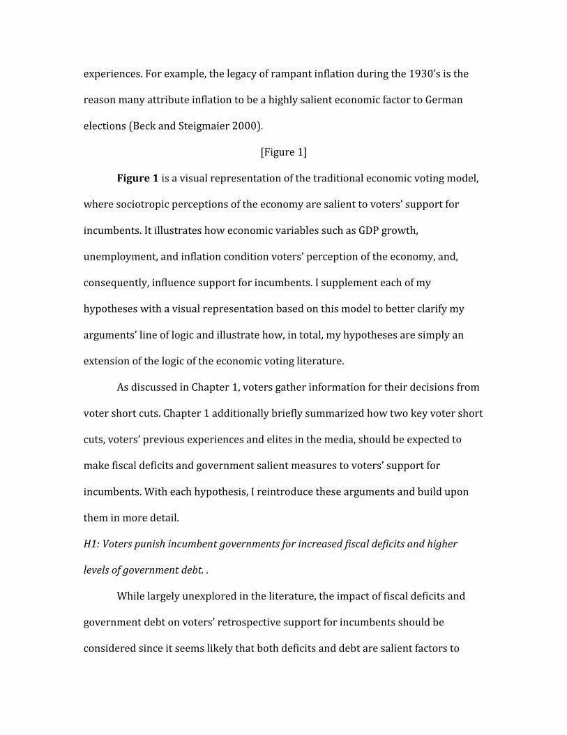
Figure 1 is a visual representation of the traditional economic voting model,

where sociotropic perceptions of the economy are salient to voters’ support for

incumbents. It illustrates how economic variables such as GDP growth,

unemployment, and inflation condition voters’ perception of the economy, and,

consequently, influence support for incumbents. I supplement each of my

hypotheses with a visual representation based on this model to better clarify my

arguments’ line of logic and illustrate how, in total, my hypotheses are simply an

extension of the logic of the economic voting literature.

As discussed in Chapter 1, voters gather information for their decisions from

voter short cuts. Chapter 1 additionally briefly summarized how two key voter short

cuts, voters’ previous experiences and elites in the media, should be expected to

make fiscal deficits and government salient measures to voters’ support for

incumbents. With each hypothesis, I reintroduce these arguments and build upon

them in more detail.

H1: Voters punish incumbent governments for increased fiscal deficits and higher

levels of government debt. .

While largely unexplored in the literature, the impact of fiscal deficits and

government debt on voters’ retrospective support for incumbents should be

considered since it seems likely that both deficits and debt are salient factors to

voters’ decision making. Nonetheless, if fiscal deficits and government debt are

salient to voting decisions, what is the expected direction of impact? I contend that

voters’ everyday life experiences, a very influential information shot cut, generally

shape a negative view of negative budget surpluses, often labeled fiscal deficits. In

general, voters cannot over allocate their income for a given month and have to

sometimes make difficult cost benefit assessments on where to spend their income.

Viewing fiscal deficits and government debt through this lens, voters could be

expected, in the general case, to hold incumbent governments to a similar standard.

If true, voters’ should punish incumbents for increases in fiscal deficits and

government debt.

[Figure 2]

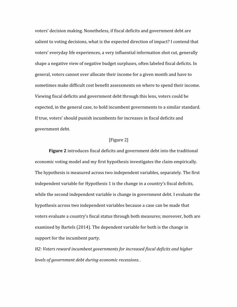
Figure 2 introduces fiscal deficits and government debt into the traditional

economic voting model and my first hypothesis investigates the claim empirically.

The hypothesis is measured across two independent variables, separately. The first

independent variable for Hypothesis 1 is the change in a country’s fiscal deficits,

while the second independent variable is change in government debt. I evaluate the

hypothesis across two independent variables because a case can be made that

voters evaluate a country’s fiscal status through both measures; moreover, both are

examined by Bartels (2014). The dependent variable for both is the change in

support for the incumbent party.

H2: Voters reward incumbent governments for increased fiscal deficits and higher

levels of government debt during economic recessions. .

However, sometimes individuals accumulate higher levels of debt in the

short term at certain points of the life cycle. For example, individuals take out

mortgages to purchase homes and parents take out loans to send children to college.

Most often, these higher levels of personal debt do not negatively impact an

individual so as long as they can pay off the debt when normal circumstances return.

Similarly, many economists agree that during economic recessions,

governments should run budget deficits to invest in infrastructure and/or cut taxes,

while limiting deficits during economic expansions.1 Economists influence other

voter information short cuts, their reports often are cited in policy makers’ speeches

and in the media, and they could be considered information short cuts themselves to

some voters. If true, this begs the question: does the common economic view that

deficits are sometimes beneficial and sometimes harmful conditional on the

business cycle itself condition voters’ treatment of deficits and government debt

dependent on the business cycle?

[Figure 3]

Figure 3 introduces the business cycle as conditioning the impact of fiscal

deficits and government debt on voters. Hypothesis 2 examines this question

empirically by examining the interactive effects of a dummy variable for whether or

not the country was in a recession on the effects of fiscal deficits and government

debt on incumbent vote share.

H3: Voters punish deficits more during recessions that overlap with financial crises.

1 For example, early in the 2008 financial crises, the IMF called on countries to prioritize fiscal space on target investments, transfers and limited tax cuts. For more information, see Laeven and Valencia (2008).

Even so, scholarly work from the 2008 financial crises presents the

possibility that voters’ reward/punishment of deficits and government debt may be

even more nuanced. Bartels (2014) finds that voters generally rewarded increases

in discretionary spending financed by debt (i.e. stimulus), but punished incumbents

for debt used to finance bailouts and nationalizations (31). Altogether, these

findings suggest that voters may be less willing to support deficits used to bailout

actors they perceive as causing a crises (i.e. banks), while maintaining a

commitment to programs that are aimed to benefit the overall economy.

[Figure 4]

Figure 4 introduces bailouts and nationalizations as inputs into fiscal deficits

and government debt. However, this explanation presents an evaluation problem:

voters only have one vote. In other words, they cannot split their vote to support

deficits used to finance stimulus, but not support deficit financed

bailouts/nationalizations. While more micro­level research is needed on whether

voter support for deficits is conditioned by the origins of deficits – stimulus vs.

bailouts­­new survey research of this kind is outside the scope of this paper.

However, I do address the issue of whether voters in aggregate are less likely to

support fiscal deficits and government debt when the actors perceived to start the

crises are more identifiable. Since part of the definition of a financial crisis is

government intervention into the financial sector, I explore if the effects of fiscal

deficits and government debt are increased by if the election took place during a

financial crises (Reinhart and Rogoff 2009). Hypothesis 3 does so empirically by

examining the interactive effects of a financial crises dummy variable on the effect of

fiscal deficits and government debt on incumbent vote share.

Sample Selection

I examine 164 elections from a pool of 19 developed, high income countries

from 1975­2012. I include the same countries Duch and Stevenson (2006) because

their large scale, comparative work found results indicative of economic voting

using survey data as well as election results. I restrict my sample to countries that

have been tested before in the literature since introducing other countries would

require first establishing that economic voting occurs. While I hope to explore

these effects in other nations at a later time, these pursuits are worthy of projects

in of themselves: the literature has spent decades expanding the economic voting

model to new countries. Likewise, while I do hope to examine the role of fiscal

deficits and government debt in low income countries one day, the effects of

economic voting in these countries is not as well as established as it is in developed

nations (Lewis and Beck 2000). Moreover, financial data in non­developed

countries is less reliable and fiscal policy data even less so.

The depth of data available for the financial statistics restricts the time

period to 1975. While a greater time span would yield more conclusive results, 37

years provides enough election variance (n=164) to sufficiently evaluate my

hypothesis.

Operationalization of Concepts

The dependent variable for my study is Δ INCUMBENT VOTE, which is

defined as the change in the vote share of the incumbent government. Election

results are extracted from the Database of Political Institutions (DPI), published by

the World Bank. When not available, data is supplemented from local sources. The

DPI is an exhaustive source for institutional analysis and is an authoritative source

for data in political science. I analyze lower house results as it generally provides

more data points and thus more variance. Moreover, many economic voting studies

utilize lower house results and it is the unit of analysis of choice for Bartels (2014).

Survey level data would be the most accurate representation of voter

opinion, but it is very costly to obtain this data on the scale this paper evaluates.

Comparing incumbent electoral performance in elections across consecutive

elections is the next best measure and a standard manner of evaluating incumbent

support in the economic voting literature (Lewis and Beck 2000).

In order to determine incumbency, I utilize the DPI’s definition: in

parliamentarian systems, the incumbent party is defined as the party that received

the highest percentage of the previous election’s vote. In presidential systems, the

President’s party is treated as the incumbent party regardless of the previous

election. This is standard practice in comparative studies (see Bartels 2014).

My first key variable of interest is DEFICIT, which is defined as the year on

year change in central government balance (negative budget surplus) as a

percentage of GDP. The second variable of interest is DEBT which is defined on the

year on year change in total government debt as a percentage of GDP. Fiscal deficit

and government debt data is extracted from OECD National Accounts Database and

is supplemented by the IMF International Financial Statistics Database, both

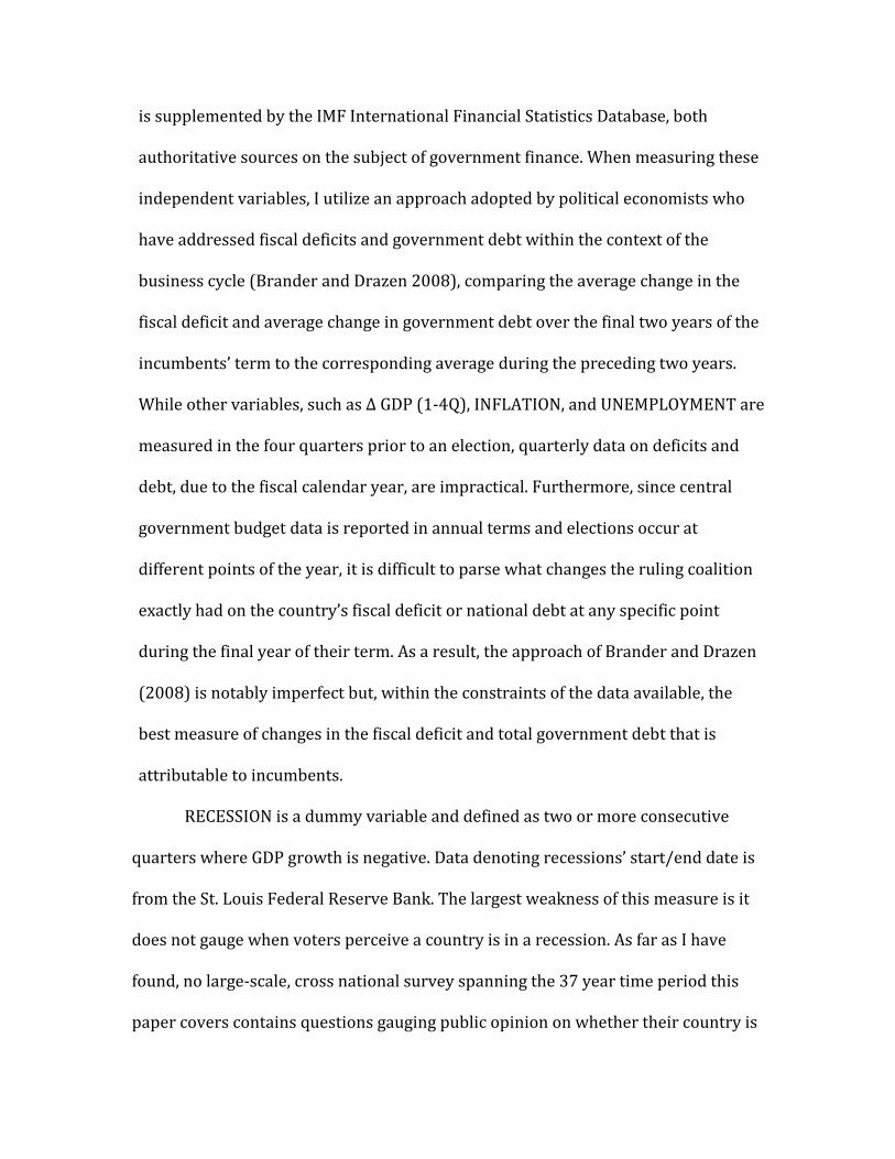
authoritative sources on the subject of government finance. When measuring these

independent variables, I utilize an approach adopted by political economists who

have addressed fiscal deficits and government debt within the context of the

business cycle (Brander and Drazen 2008), comparing the average change in the

fiscal deficit and average change in government debt over the final two years of the

incumbents’ term to the corresponding average during the preceding two years.

While other variables, such as Δ GDP (1­4Q), INFLATION, and UNEMPLOYMENT are

measured in the four quarters prior to an election, quarterly data on deficits and

debt, due to the fiscal calendar year, are impractical. Furthermore, since central

government budget data is reported in annual terms and elections occur at

different points of the year, it is difficult to parse what changes the ruling coalition

exactly had on the country’s fiscal deficit or national debt at any specific point

during the final year of their term. As a result, the approach of Brander and Drazen

(2008) is notably imperfect but, within the constraints of the data available, the

best measure of changes in the fiscal deficit and total government debt that is

attributable to incumbents.

RECESSION is a dummy variable and defined as two or more consecutive

quarters where GDP growth is negative. Data denoting recessions’ start/end date is

from the St. Louis Federal Reserve Bank. The largest weakness of this measure is it

does not gauge when voters perceive a country is in a recession. As far as I have

found, no large­scale, cross national survey spanning the 37 year time period this

paper covers contains questions gauging public opinion on whether their country is

in a recession. Thus, while future work should attempt to examine this line of

reasoning utilizing more in depth survey techniques, I rely on the technical

definition employed by economists (Hall 1993)

CRISES are defined utilizing the Reinhart and Rogoff (2009) definition for

banking crises in This Time is Different (8). Likewise, data denoting the time period

of crises is from the This Time is Different data set. Countries without crises dates

are omitted from this part of the analysis. Reinhart and Rogoff (2009) define

banking crises as occurring when 1) a run on a bank leads to the closure, merging

or takeover by the government or 2) if there is no run on the banks, the

government closing, merging, or taking over an important financial institutions.

Reinhart and Rogoff (2009) discuss how there are other, more ideal measures of

banking crises, such as the relative price of banks stock. However, the time series

data on these more accurate measures is very limited and not consistent across

countries. Furthermore, Reinhart and Rogoff (2009) is an emerging authoritative

source on the history of financial crises. The breadth and reliability of the

scholarship justifies utilizing the measure despite its limitations.

I use two groups of CONTROL variables that have been established in

economic voting literature. My economic CONTROL variables are Δ GDP (1­4Q) and

INFLATION. Δ GDP (1­4Q) is defined as the percent change in gross domestic

product in the four quarters prior to the election. INFLATION is the change in

percent of the consumer price index during the election year.2 Data on Δ GDP (1­

2 Unemployment is another measure that has been established in the literature as impacting voters’ retrospective evaluation of incumbents (see Lewis and Beck 2000). However, unemployment is

4Q) and INFLATION is taken from the OECD National Accounts Database and is

supplemented by the IMF International Financial Statistics Database. I have

selected these variables since the previous economic voting literature has

established them as having a significant effect independently and jointly on voters

support for incumbents (Lewis and Beck 2000).

Institutional CONTROL variables include YEARS and IDEALOGY. YEARS is the

number of quarters the incumbents have held office. IDEOLOGY is the partisanship

ranking of the incumbent government. It is a dummy variable, with 1=right leaning

government and 2=left leaning government. These are standard definitions for

these variables in the comparative economic voting literature. It is important to

include these variables, as each as emerged has been raised as non­economic

factors that could drive retrospective voting (Lewis and Beck 2000).

Empirical Models

Below I introduce my regression models for economic voting that include

DEFICIT and DEBT. The outcome variable for each is Δ INCUMBENT VOTE. The

results for each are evaluated using OLS (Ordinary Least Square) regression with

White­Huber (robust) standard errors. Scatter plots of the relationship are also

presented in my analysis section to supplement the regression analyses.

𝑦𝑖= 𝛽1+𝛽2+𝛽3+𝛽4(𝑋1∗𝑋2)+𝛽5(𝑋1∗𝑋3)+𝜀𝑖

omitted from this analysis since it is highly correlated with GDP and, thus, subjects my empirical model to high levels of co­linearity.

Above is my regression model for economic voting including DEFICIT. 𝛾𝑖 is Δ

INCUMBENT VOTE . 𝛽1 represents DEFICIT. 𝛽2 is the dummy variable RECESSION

and 𝛽3 is the dummy variable CRISES. 𝛽4(𝑋1 ∗ 𝑋2) is an interaction term DEFICIT *

RECESSION and 𝛽4(𝑋1 ∗ 𝑋3) is an interaction term DEFICIT * CRISES. 𝜀𝑖 represents

both my economic and institutional CONTROL variables: Δ GDP (1­4Q), INFLATION,

YEARS, and IDEAOLOGY.

𝑦𝑖= 𝛽1+𝛽2+𝛽3+𝛽4(𝑋1∗𝑋2)+𝛽5(𝑋1∗𝑋3)+𝜀𝑖

Above is my second regression model which is very similar to my first model

but includes DEBT instead of DEFICIT. 𝛾𝑖 is Δ INCUMBENT VOTE .𝛽1 represents

DEBT. 𝛽2 is the dummy variable RECESSION and 𝛽3 is the dummy variable CRISES.

𝛽4(𝑋1 ∗ 𝑋2) is an interaction term DEBT * RECESSION and 𝛽4(𝑋1 ∗ 𝑋3) is an

interaction term DEBT * CRISES. 𝜀𝑖 represents both my economic and institutional

CONTROL variables: Δ GDP (1­4Q) , INFLATION, YEARS, and IDEAOLOGY.

When assessing the predicative power of these models, evidence that

indicate independent variables have a significant effect is considered good evidence

suggestive of a relationship. Significance is defined as coefficients with a p value

<.05. In addition, I assess the explanatory power of the deficits variable in each

hypothesis, with a R2 > .25 being the benchmark to determine if a variable has high

explanatory power.

One potential obstacle to this paper’s causal inference is the endogenous

relationship between Δ GDP (1­4Q) and DEFICIT as well as between Δ GDP (1­4Q)

and DEBT. As discussed in Bartels (2014), DEFICIT and DEBT often increase when

Δ GDP (1­4Q) decreases since governments often expand fiscal policy to fight

economic downturns. As a result, it does make it difficult to parse out the

independent effects of Δ GDP (1­4Q), DEFICIT and DEBT since voters could be

reacting to either. My research design attempts to account for this challenge by

utilizing a multivariate regression approach in a similar fashion to Bartels (2014)

.By including both economic and institutional CONTROL variables, I make the best

case within the constraints of the literature to examine if DEFICIT and DEBT

independently influence incumbent support.

Another question my empirical approach raises is that it assumes economic

voting to in fact be the baseline behavior of voters. Some may critique this

assumption, claiming that elections are retrospective evaluations of independent

(sometimes random) events instead of being focused on sociotropic economic

conditions. Altogether, this line of reasoning is well founded in the literature (see

Achen and Bartels 2002 or Healy, Malhotra, and Cecilia 2010). Nonetheless, while a

worthwhile debate, this project does not seek to inform the economic voting vs.

illogical retrospective discussion. Instead, it explores if DEFICIT or DEBT are

influential within the economic voting framework. Consequently, for the purposes

of this study, economic voting is assumed to be an accurate model of voting

behavior

Conclusion

In this chapter, I augmented the traditional economic voting model by

incorporating fiscal deficits and government debt as additional influences on voting

behavior. I articulated my argument that deficits and debt are salient to voting

decisions since they relate to the same voter short cuts as traditional economic

voting variables. In addition, I developed three testable hypotheses that emerge

from my theory and explained my empirical strategy for analyzing these arguments.

Having established my question, theory, and empirical strategy, I now

proceed to analyze the results. Chapter3 presents my analysis and Chapter 4

outlines several conclusions I draw from the results.

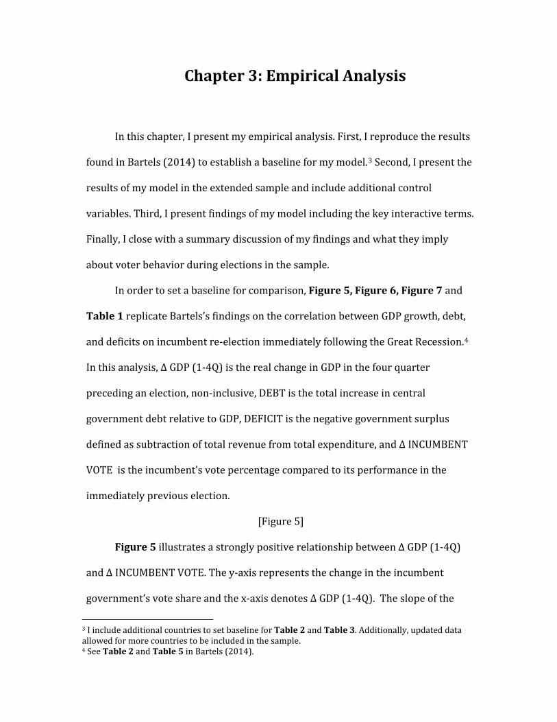
Chapter 3: Empirical Analysis

In this chapter, I present my empirical analysis. First, I reproduce the results

found in Bartels (2014) to establish a baseline for my model.3 Second, I present the

results of my model in the extended sample and include additional control

variables. Third, I present findings of my model including the key interactive terms.

Finally, I close with a summary discussion of my findings and what they imply

about voter behavior during elections in the sample.

In order to set a baseline for comparison, Figure 5, Figure 6, Figure 7 and

Table 1 replicate Bartels’s findings on the correlation between GDP growth, debt,

and deficits on incumbent re­election immediately following the Great Recession.4

In this analysis, Δ GDP (1­4Q) is the real change in GDP in the four quarter

preceding an election, non­inclusive, DEBT is the total increase in central

government debt relative to GDP, DEFICIT is the negative government surplus

defined as subtraction of total revenue from total expenditure, and Δ INCUMBENT

VOTE is the incumbent’s vote percentage compared to its performance in the

immediately previous election.

[Figure 5]

Figure 5 illustrates a strongly positive relationship between Δ GDP (1­4Q)

and Δ INCUMBENT VOTE. The y­axis represents the change in the incumbent

government’s vote share and the x­axis denotes Δ GDP (1­4Q). The slope of the

3 I include additional countries to set baseline for Table 2 and Table 3. Additionally, updated data allowed for more countries to be included in the sample. 4 See Table 2 and Table 5 in Bartels (2014).

regression line is positive and fairly steep, suggesting a strong positive relationship

between Δ GDP (1­4Q) and Δ INCUMBENT VOTE share during and immediately

following the crises.

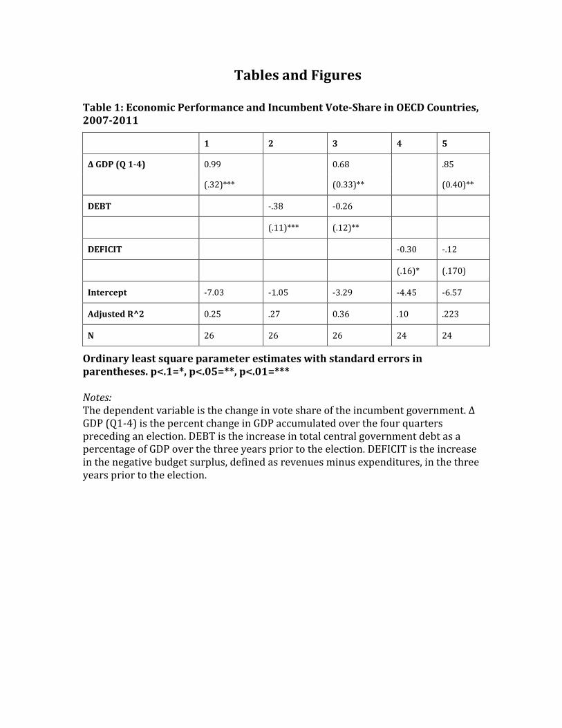
Model 1 in Table 1 supports the findings of Figure 5. Δ GDP (1­4Q) yields a

statistically significant coefficient of ~0.99. The level of significance leads one to

conclude that there is a strong correlation between the two variables; the odds that

the relationship is due to chance are less than 5%. An adjusted R^2 value of .25

means that Model 1 “explains” ~25% of the variance in incumbent vote share.

Moreover, the degree and strength of this coefficient suggests that GDP growth in a

country is a very strong predictor of electoral performance during and following

the Great Recession. For example, we would expect a country that sustained a 4%

loss in GDP during a year to nearly lose 4% of support in their next election.

[Figure 6]

Figure 6 illustrates my replication of Bartels’s finding of a negative

relationship between DEBT and Δ INCUMBENT VOTE. The y­axis represents the

change in the incumbent government’s vote share and the x­axis denotes DEBT.

The slope of the regression line is negative and fairly steep, implying a negative

correlation between DEBT and incumbent government’s performance. In addition,

the scatter of the data is reasonably clustered around the regression line,

predicting that simple bivariate model of the variables will have some explanatory

power.

Model 2 and Model 3 in Table 1 support this analysis. DEBT is negatively

correlated with Δ INCUMBENT VOTE and the coefficient of ~ ­.38 is significant.

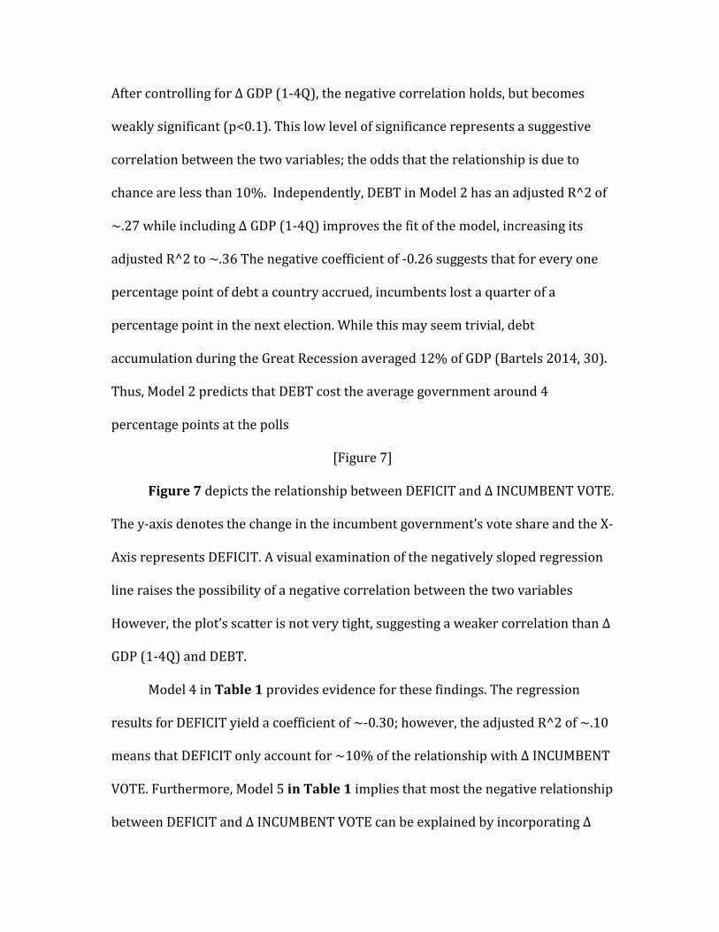
After controlling for Δ GDP (1­4Q), the negative correlation holds, but becomes

weakly significant (p<0.1). This low level of significance represents a suggestive

correlation between the two variables; the odds that the relationship is due to

chance are less than 10%. Independently, DEBT in Model 2 has an adjusted R^2 of

~.27 while including Δ GDP (1­4Q) improves the fit of the model, increasing its

adjusted R^2 to ~.36 The negative coefficient of ­0.26 suggests that for every one

percentage point of debt a country accrued, incumbents lost a quarter of a

percentage point in the next election. While this may seem trivial, debt

accumulation during the Great Recession averaged 12% of GDP (Bartels 2014, 30).

Thus, Model 2 predicts that DEBT cost the average government around 4

percentage points at the polls

[Figure 7]

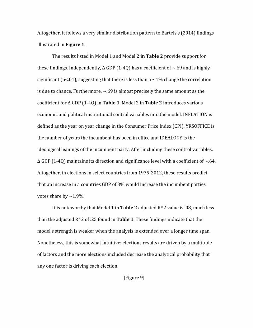
Figure 7 depicts the relationship between DEFICIT and Δ INCUMBENT VOTE.

The y­axis denotes the change in the incumbent government’s vote share and the X­

Axis represents DEFICIT. A visual examination of the negatively sloped regression

line raises the possibility of a negative correlation between the two variables

However, the plot’s scatter is not very tight, suggesting a weaker correlation than Δ

GDP (1­4Q) and DEBT.

Model 4 in Table 1 provides evidence for these findings. The regression

results for DEFICIT yield a coefficient of ~­0.30; however, the adjusted R^2 of ~.10

means that DEFICIT only account for ~10% of the relationship with Δ INCUMBENT

VOTE. Furthermore, Model 5 in Table 1 implies that most the negative relationship

between DEFICIT and Δ INCUMBENT VOTE can be explained by incorporating Δ

GDP (1­4Q) into the model. After Δ GDP (1­4Q) is factored in, DEFICIT remains

negatively correlated, but loses its statistical significance. As a result we cannot

conclude with any level of conclusiveness that the negative relationship between

DEFICIT and Δ INCUMBENT VOTE is not due to chance.

The varying strength in the coefficients between Δ GDP (1­4Q) and DEBT

illustrate the difficult choices faced by politicians during the financial crises: GDP

growth was rewarded more than debt was punished, but if the GDP growth did not

come fast enough or voters did not establish a link between fiscal policy and

economic growth, accumulating debt could cost a government greatly at the next

election.

Furthermore, the contrasting strength and significance levels between DEBT

and DEFICIT is noteworthy. On one hand, it is somewhat perplexing since DEBT is

largely a function of year­to­year DEFICIT. On the other hand, the divergence could

also be suggestive of differentiation in the voter treatment of DEBT and DEFICIT.

However, the small sample of size found in the models in Table 1 limits the degree

of support for different voter treatment of DEBT and DEFICIT. Next, I extend

Bartels’s (2014) model back to 1975, adding a few additional control variables, and

keep an eye to see if any of these trends hold in the larger sample size.

[Figure 8]

Figure 8 is a scatter plot distribution of the correlation between Δ GDP (1­

4Q) and Δ INCUMBENT VOTE from 1975 – 2012. It’s fairly steep and positive slope

imply a strong, positive correlation between Δ GDP (1­4Q) and Δ INCUMBENT VOTE.

Altogether, it follows a very similar distribution pattern to Bartels’s (2014) findings

illustrated in Figure 1.

The results listed in Model 1 and Model 2 in Table 2 provide support for

these findings. Independently, Δ GDP (1­4Q) has a coefficient of ~.69 and is highly

significant (p<.01), suggesting that there is less than a ~1% change the correlation

is due to chance. Furthermore, ~.69 is almost precisely the same amount as the

coefficient for Δ GDP (1­4Q) in Table 1. Model 2 in Table 2 introduces various

economic and political institutional control variables into the model. INFLATION is

defined as the year on year change in the Consumer Price Index (CPI), YRSOFFICE is

the number of years the incumbent has been in office and IDEALOGY is the

ideological leanings of the incumbent party. After including these control variables,

Δ GDP (1­4Q) maintains its direction and significance level with a coefficient of ~.64.

Altogether, in elections in select countries from 1975­2012, these results predict

that an increase in a countries GDP of 3% would increase the incumbent parties

votes share by ~1.9%.

It is noteworthy that Model 1 in Table 2 adjusted R^2 value is .08, much less

than the adjusted R^2 of .25 found in Table 1. These findings indicate that the

model’s strength is weaker when the analysis is extended over a longer time span.

Nonetheless, this is somewhat intuitive: elections results are driven by a multitude

of factors and the more elections included decrease the analytical probability that

any one factor is driving each election.

[Figure 9]

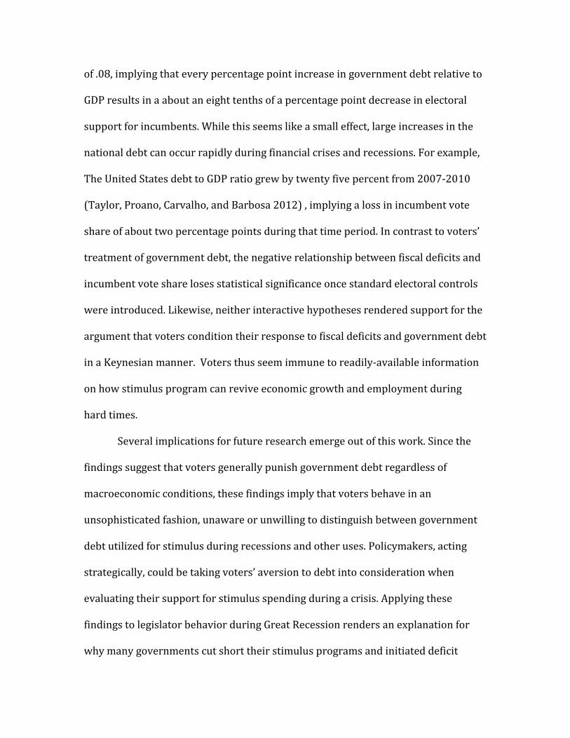
Figure 9 illustrates the correlation between DEBT and Δ INCUMBENT VOTE

for the extend sample, 1975 ­ 2012. The negative slope of the regression line and

over fit of the correlation imply a fairly strong, negative relationship between DEBT

and Δ INCUMBENT VOTE. These results are similar to the results found replicating

Bartels’s findings in Figure 2.

The regression results found in Table 2 support these comparisons. The

bivariate correlation between DEBT and Δ INCUMBENT VOTE is negative and yields

a coefficient of ~­.05. Moreover, its findings are significant (p<.05), suggesting that

there is less than 5% probability that the correlation is due to chance. However, the

adjusted R^2 of Model 3 in Table 2 is lower than Model 2 in Table 1 at ~.08,

implying the correlation explains approximately only 8% of the variance. These

results imply a negative relationship similar to those found in Table 1, but with

much weaker explanatory power.

However, introducing other control variables improves the overall fit of the

model. Model 4 indicates the results of the regression analysis when including Δ

GDP (1­4Q) and Model 8 introduces all the economic and political control variables

utilized. In each case DEBT maintains its negative direction and significance level of

p<.05. The most suggestive results are found in the model described by Column 8,

with DEBT yielding a coefficient of ~­.10 and the models adjusted R^2 value

reaching .11. These findings suggest that GDP (1­4Q) is again positively correlated

with re­election and the strongest predictor of reelection, but that also a 1%

increase in national debt is correlated with a loss of .10 of vote share. While a

smaller coefficient than Δ GDP, the results imply an electoral impact as national debt

can often increase by 10% points or more during the course of an incumbent’s term.

[Figure 10]

The correlation between DEFICITS and Δ INCUMBENT VOTE is illustrated in

the scatter plot in Figure 10. Since the slope of the regression line is negative, but

the scatter is not tight around the regression line. Altogether, the scatter plot

suggests a weak negative relationship. Noteworthy, the fit of the correlation does

hold a pattern very similar that during the Great Recession found in Figure 3.

Model 5, Model 6, and Model 7 in Table 2 are my three models including the

DEFICIT and DEBT variable. Each of these Models measures the claims of

Hypothesis 1 and Hypothesis 2: voters, contextualizing DEFICIT and DEBT in their

own circumstances, generally punish incumbents for increased DEFICIT and DEBT.

Model 5 lays out the initial regression analysis between DEFICIS and Δ INCUMBENT

VOTE and supports the findings of Figure 6. DEFICIT has a coefficient of ~­.38 and

is very significant (p<.01). Initially, this implies a strong negative relationship,

suggesting that 5% increase in a countries deficit as a percentage of GDP is

correlated with a loss of 2% of vote share for incumbent parties. However, when

included with models introducing economic and political control variables in Model

6 and Model 8 in Table 2, DEFICIT loses its strength and significance. As a result,

very little can be drawn analytically from these results with regards to assessing the

impact of DEFICIT on Incumbent Electoral Share.

In summary, the results of Table 2 largely mirror those found in Table 1.

GDP growth is best predictor of incumbent election success and yields the largest

coefficient magnitude. These findings are consistent with the argument that

economic retrospective voting contingent upon growth is a dominant factor

influencing voter’s support on incumbents. In addition, while it’s overall effect is

diminished, central government debt is negatively correlated with incumbent re­

election in the extended sample. These results implies a stronger case for the

presence of a “Keynesian Tradeoff”: voters punish debt, but not nearly as much as

they may reward growth. Finally, similar to Bartels’s (2014) findings and my

replication of his results in Table 1, DEFICIT is not conclusively correlated with

incumbent performance.

The results of Table provide support for Hypothesis 1 contingent upon how

one operationalizes examines the budgetary consequences of Fiscal Policy. If the

more accurate measure is DEFICIT, the lack of significance of the results mean that

these models do not provide substantial support that voters punish increased

DEFICITS. Nonetheless, the evidence that consistently punish DEBT is statistically

significant and negative, ultimately providing partial support for Hypothesis 1.

An intriguing result from the models in Table 2 is the continuance of a­

symmetry in effect of DEFICIT and DEBT on incumbent re­election. Since DEBT is

largely a function of accumulated DEFICIT, it initially seems odd that voters would

differentiate their treatment of both. However, under the assumption that voters

examine the economy through the prism of their own financial circumstances, the

phycology and economic behavior literature provides some theoretical background

for this bifurcated treatment. I discuss these possibilities and their opportunities for

future research in Chapter 4.

Table 3 introduces four interactions terms CRISES * DEBT, CRISES *

DEFICIT, RECESSION * DEBT, and RECESSION * DEFICIT. These interact terms

evaluate Hypothesis 2 and Hypothesis 3 that voters condition their punishment of

DEBT and DEFICIT on macro­economic conditions. According to Hypothesis 1

RECESSIONS are expected to diminish the negative impact since voters could be

expected to support DEFICIT and DEBT financed stimulus during hard times. In

contrast, Hypothesis 3 claims that CRISES should expected to increase the

magnitude that voters punish DEBT and DEFICIT since bailouts often go to

institutions that are perceived to start the crises. In each, CRISES is defined utilizing

the Reinhart and Rogoff (2009) definition of a financial crisis, which they define as

being preceded one or more of the following: a banking crises, currency crash,

sovereign debt or extern debt restructuring, inflation crises or stock market crash.

RECESSION is defined the period in the business cycle between the peak of

economic activity and its trough, following the NBER definition of recession.5

In each of the Models in Table 3 the coefficient of the interaction term is

negative, implying that the presence of a CRISES or RECESSION diminishes the

negative effect of DEBT or DEFICIT on incumbent re­election. Nonetheless, none of

the coefficients reaches significance, meaning that the probability that these results

are due to chance is too high to conclude any correlation. As a result, none of the

Models in Table 3 provide support for either Hypothesis 2 or Hypothesis 3.

Overall, these findings do not lend support to the claim that electorate’s view

on DEBT and DEFICIT is conditioned by macroeconomic conditions. Instead, they

5 For more information, see Feldstein et al. (2003)

suggest a voter who continually punishes incumbents for DEBT accumulation and

who displays no consistent attitude towards DEFICIT. As a result, it is possible that

voter’s punishment of DEBT could be constant, even during crises. This poses a

potential constraint upon policymakers: if leaders deem accumulating debt in the

short run as a necessary/justified step to stimulate the economy, they may

reconsider doing so or scale down the size of their debt financed stimulus if they

think that electorates will punish them.

In conclusion, the correlations between ΔGDP (1­4Q), DEBT, DEFICIT and Δ

INCUMBENT VOTE found in Bartels (2014) hold in direction and significance in the

extended sample. The strongest predictor of election results remains ΔGDP (1­4Q).

These findings are consistent with the argument that voters engage in retrospective,

economic voting. Simply put, voters reward incumbents who preside over economic

growth prior to elections and punish those who do not.

DEBT is additionally negatively correlated with Incumbent Support, yielding

a coefficient of ~.10 in the most encompassing model. While a smaller effect than in

Bartels (2014), these results still imply that that extent that voters may punish

DEBT could be quite impactful. There are many cases when national DEBT has

changed by 10% of GDP or more during an incumbent’s term, especially during

recessions and wars. If this occurs, the most encompassing model in the extended

sample would predict a 1% loss in vote share due to increases in DEBT.

On the other hand, these results do not provide support for the position that

voters differentiate between good economic times and bad, with all DEBT and

DEFICIS interact terms failing to reach significance. Since most economists argue

that debt financed stimulus in recessions is needed, these results imply a possible

constraint on the extent to which politicians may leverage debt to implement

stimulus packages during hard times. Consequently, these results imply an

economic unsophisticated voter: one who greatly rewards economic growth, but

may be blind to the policies necessary to make it occur.

Chapter 4 presents my conclusions from this analysis. It discusses the

implications of the results and seeks to place them within the larger economic

voting literature. Additionally, it presents the limitations of my findings and ideas

for future research.

Chapter 4: Conclusion

Since its introduction during the Great Depression, Keynesian demand

management has been at the forefront of policy debates during crises. While

economists have focused on the effectiveness of fiscal stimulus programs, few

scholars have examined the political economy of the fiscal deficits and government

debt that is used to finance Keynesian stimulus packages. My thesis has addressed

this gap in the literature by exploring the extent to which voters support fiscal

deficits and government debts that are used to finance stimulus programs during

recessions. In this section, I discuss my contributions to the literature, the

limitations of my findings, and the implications of my work for the future research

agenda.

My primary contribution to the literature has been expanding the traditional

economic voting model to include fiscal deficits and government debt. To evaluate

the reliability and accuracy of my expanded model, I have extended Bartels (2014)

analysis of retrospective economic voting during the Great Recession across a

longer time span, with an eye towards examining electoral punishment (support) of

government debt and deficits. In addition, I introduced and empirically assessed

interactive hypotheses to see if voters mediate their treatment of both fiscal deficits

and government debt during recessions in a “Keynesian” fashion.

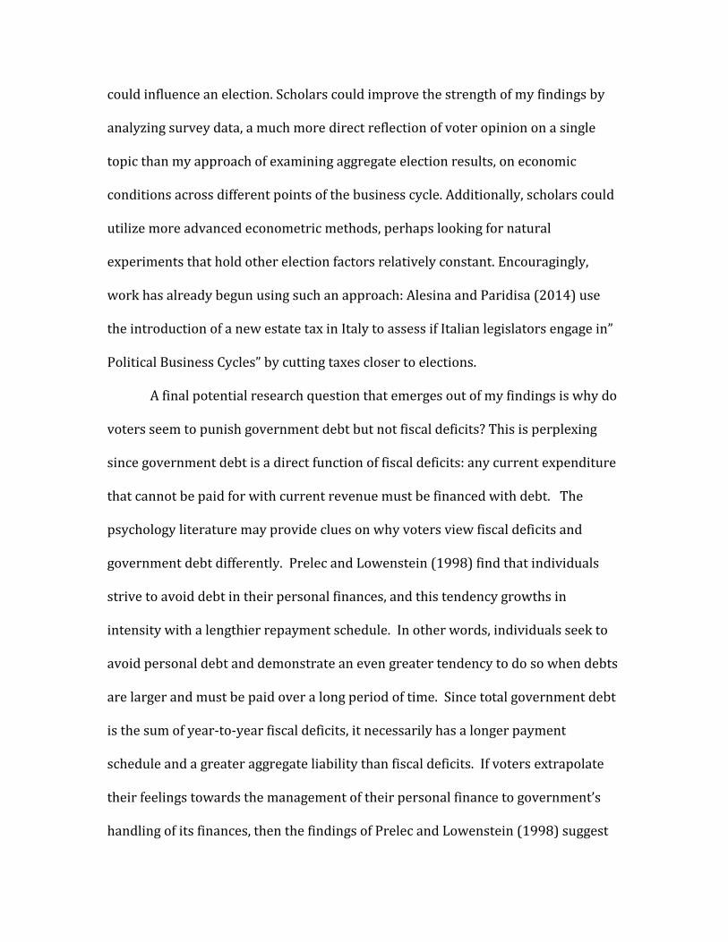
The results suggest that voters punish debt regardless of whether it is used

to fund stimulus programs during recessions or not. When including standard

electoral control variables in my sample, government debt has a negative coefficient

of .08, implying that every percentage point increase in government debt relative to

GDP results in a about an eight tenths of a percentage point decrease in electoral

support for incumbents. While this seems like a small effect, large increases in the

national debt can occur rapidly during financial crises and recessions. For example,

The United States debt to GDP ratio grew by twenty five percent from 2007­2010

(Taylor, Proano, Carvalho, and Barbosa 2012) , implying a loss in incumbent vote

share of about two percentage points during that time period. In contrast to voters’

treatment of government debt, the negative relationship between fiscal deficits and

incumbent vote share loses statistical significance once standard electoral controls

were introduced. Likewise, neither interactive hypotheses rendered support for the

argument that voters condition their response to fiscal deficits and government debt

in a Keynesian manner. Voters thus seem immune to readily­available information

on how stimulus program can revive economic growth and employment during

hard times.

Several implications for future research emerge out of this work. Since the

findings suggest that voters generally punish government debt regardless of

macroeconomic conditions, these findings imply that voters behave in an

unsophisticated fashion, unaware or unwilling to distinguish between government

debt utilized for stimulus during recessions and other uses. Policymakers, acting

strategically, could be taking voters’ aversion to debt into consideration when

evaluating their support for stimulus spending during a crisis. Applying these

findings to legislator behavior during Great Recession renders an explanation for

why many governments cut short their stimulus programs and initiated deficit

reducing reforms: legislators may have been cautious to take on large debt loads for

stimulus out of fear of political retribution by voters.

Nonetheless, the results do, for the most part, support findings in the

retrospective economic voting literature. Similar to Bartels (2014), GDP growth was

found to be the most important predicator of incumbent electoral success. GDP’s

coefficient of .52 is much greater than government debt’s ­.08, suggesting that a one

percent increase in GDP is rewarded more than a one percent reduction in the

national debt. While this study provides no evidence for a “Keynesian voter”, these

results do suggest a sort of “Keynesian tradeoff” faces legislators governing during

economic crises since growth is rewarded more than debt is punished. A future

puzzle for scholars to explore is why voters consistently reward economic growth,

but do not appear to support stimulus programs that a majority of economists agree

will increase GDP.

An overarching limitation of this study is its reliance on the assumption that

retrospective economic voting is the best model of voting behavior. This is not a

settled debate in the scholarly research. Evidence from studies has pointed towards

voters holding incumbent responsible for irrational, non­economic events including

shark attacks and football games (Achen and Bartels 2004;Healy, Malhotra and Mo

2010). However, the findings of this study do contribute to the discussion within the

parameters of economic voting, a growing literature within political economy.

However, many of the limitations of my study help drive future possibilities

for research. The greatest weakness of my empirical approach is my reliance on OLS

Regression since it is almost impossible to identify and control for every factor that

could influence an election. Scholars could improve the strength of my findings by

analyzing survey data, a much more direct reflection of voter opinion on a single

topic than my approach of examining aggregate election results, on economic

conditions across different points of the business cycle. Additionally, scholars could

utilize more advanced econometric methods, perhaps looking for natural

experiments that hold other election factors relatively constant. Encouragingly,

work has already begun using such an approach: Alesina and Paridisa (2014) use

the introduction of a new estate tax in Italy to assess if Italian legislators engage in”

Political Business Cycles” by cutting taxes closer to elections.

A final potential research question that emerges out of my findings is why do

voters seem to punish government debt but not fiscal deficits? This is perplexing

since government debt is a direct function of fiscal deficits: any current expenditure

that cannot be paid for with current revenue must be financed with debt. The

psychology literature may provide clues on why voters view fiscal deficits and

government debt differently. Prelec and Lowenstein (1998) find that individuals

strive to avoid debt in their personal finances, and this tendency growths in

intensity with a lengthier repayment schedule. In other words, individuals seek to

avoid personal debt and demonstrate an even greater tendency to do so when debts

are larger and must be paid over a long period of time. Since total government debt

is the sum of year­to­year fiscal deficits, it necessarily has a longer payment

schedule and a greater aggregate liability than fiscal deficits. If voters extrapolate

their feelings towards the management of their personal finance to government’s

handling of its finances, then the findings of Prelec and Lowenstein (1998) suggest

they may be more averse to government debt then fiscal deficits. Future work could

use any of the aforementioned research strategies to explore if this speculation is

reflected in real world voting patterns.

In conclusion, voters seem immune to the logic of Keynesian demand

management and thereby punish governments for actions that seek to improve the

performance of the economy during recessions. This suggests that policymakers

will find it electorally difficult to engage in stimulus spending when it is needed

most. Finally, further analysis is vital to understanding the reasons why voters are

more opposed to large amounts of government debt than they are to the budget

deficits that are the direct cause of debts.

References

Achen, C. H., & Bartels, L. M. (2004). Blind retrospection: Electoral responses to drought, flu, and shark attacks. Alesina, A. F., Carloni, D., & Lecce, G. (2011). The electoral consequences of large fiscal adjustments (No. w17655). National Bureau of Economic Research Alesina, A., & Paradisi, M. (2014). Political budget cycles: Evidence from italian cities (No. w20570). National Bureau of Economic Research. Ansolabehere, S., Meredith, M., & Snowberg, E. (2012). Sociotropic voting and the media. Bartels, L. M. (2014). Ideology and retrospection in electoral responses to the Great Recession. Mass politics in tough times: Opinion, votes, and protest in the great recession, 185­223 Downs, A. (1957). An economic theory of democracy. Duch, R. M., & Stevenson, R. (2006). Assessing the magnitude of the economic vote over time and across nations. Electoral Studies, 25(3), 528­547. Fiorina, M. P. (1981). Retrospective voting in American national elections. Greenwood, R., Hanson, S. G., Rudolph, J. S., & Summers, L. (2014). Government Debt Management at the Zero Lower Bound Hall, R. E. (1993). Macro Theory and the Recession of 1990­1991. The American Economic Review, 275­279 Hall, R., Feldstein, M., Frankel, J., Gordon, R., Romer, C., Romer, D., & Zarnowitz, V. (2003). The NBER’s recession dating procedure. Business Cycle Dating Committee, National Bureau of Economic Research Healy, A. J., Malhotra, N., & Mo, C. H. (2010). Irrelevant events affect voters' evaluations of government performance. Proceedings of the National Academy of Sciences, 107(29), 12804­12809. Key, V. O., & Cummings, M. C. (1966). The responsible electorate (pp. 226­230). Belknap Press of Harvard University Press Kinder, D. R., & Kiewiet, D. R. (1979). Economic discontent and political behavior: The role of personal grievances and collective economic judgments in congressional voting. American Journal of Political Science, 495­527

Kinder, D. R., & Kiewiet, D. R. (1981). Sociotropic politics: the American case. British Journal of Political Science, 11(02), 129­161 Kramer, G. H. (1971). Short­term fluctuations in US voting behavior, 1896–1964. American Political Science Review, 65(01), 131­143 Laeven, L., & Valencia, F. (2008). Systemic banking crises: a new database. IMF Working Papers, 1­78. Lewis­Beck, M. S., & Stegmaier, M. (2000). Economic determinants of electoral outcomes. Annual Review of Political Science, 3(1), 183­219. Lupia, A. (1994). Shortcuts versus encyclopedias: information and voting behavior in California insurance reform elections. American Political Science Review, 88(01), 63­76 Pontusson, J., & Raess, D. (2012). How (and why) is this time different? The politics of economic crisis in Western Europe and the United States. Annual Review of Political Science, 15, 13­33. Popkin, S. L. (1993). Information shortcuts and the reasoning voter. Information, participation, and choice: An economic theory of democracy in perspective, 17­35. Prelec, D., & Loewenstein, G. (1998). The red and the black: Mental accounting of savings and debt. Marketing Science, 17(1), 4­28 Reinhart, C. M., & Rogoff, K. (2009). This time is different: eight centuries of financial folly. Princeton University Press Taylor, L., Proaño, C. R., de Carvalho, L., & Barbosa, N. (2012). Fiscal deficits, economic growth and government debt in the USA. Cambridge Journal of Economics, 36(1), 189­204. Zaller, J. (1992). The nature and origins of mass opinion. Cambridge University Press.

Tables and Figures

Table 1: Economic Performance and Incumbent Vote-Share in OECD Countries, 2007-2011

Ordinary least square parameter estimates with standard errors in parentheses. p<.1=*, p<.05=**, p<.01=*** Notes: The dependent variable is the change in vote share of the incumbent government. Δ GDP (Q1­4) is the percent change in GDP accumulated over the four quarters preceding an election. DEBT is the increase in total central government debt as a percentage of GDP over the three years prior to the election. DEFICIT is the increase in the negative budget surplus, defined as revenues minus expenditures, in the three years prior to the election.

1 2 3 4 5

Δ GDP (Q 1-4) 0.99 0.68 .85

(.32)*** (0.33)** (0.40)**

DEBT ­.38 ­0.26

(.11)*** (.12)**

DEFICIT ­0.30 ­.12

(.16)* (.170)

Intercept ­7.03 ­1.05 ­3.29 ­4.45 ­6.57

Adjusted R^2 0.25 .27 0.36 .10 .223

N 26 26 26 24 24

Table 2: Economic Performance and Incumbent Vote Share, 1975-2012 1 2 3 4 5 6 7 8 Δ GDP (Q1-4) .76 .64

.61

.65 0.52 0.62

(.20)*** (.24)***

(.21)***

(.22)*** (0.26)** (0.27)** DEBT

­.06 ­.08

­0.10

(.03)** (.036)**

(0.04)** DEFICIT

­.37 ­.07

­0.03

(0.14)*** (.16)

(0.18) INFLATION

.46

0.27 0.46

(.24)*

(0.271) (0.25) YRSOFFICE

­.39

­0.50 ­0.38

(.26)

(0.27)* (0.27) IDEAOLOGY

­.49

­0.57 ­0.48

(.65)

(0.68) (0.67) Intercept ­3.278 ­1.85 1.194 ­3.992012 ­2.756883 ­4.62 ­0.446 ­1.864 Adjusted R^2 0.087 .08 0.042 0.1144 0.034 0.0829 0.1124 0.0669 N 117 103 157 126 180 127 96 100 Ordinary least square parameter estimates with standard errors in parentheses. p<.1=*, p<.05=**, p<.01=*** Notes: The dependent variable is the change in vote share of the incumbent government. Δ GDP (Q1­4) is the percent change in GDP accumulated over the four quarters preceding an election. DEBT is the increase in total central government debt as a percentage of GDP over the three years prior to the election. DEFICIT is the increase in the negative budget surplus, defined as revenues minus expenditures, in the three years prior to the election. INFLATION is the percent change in the Consumer Price Index (C.P.I) in the three years prior to an election. YRSOFFICE is the number of years the incumbent has been in office. IDEALOGY is the ideological leaning of the incumbent government.

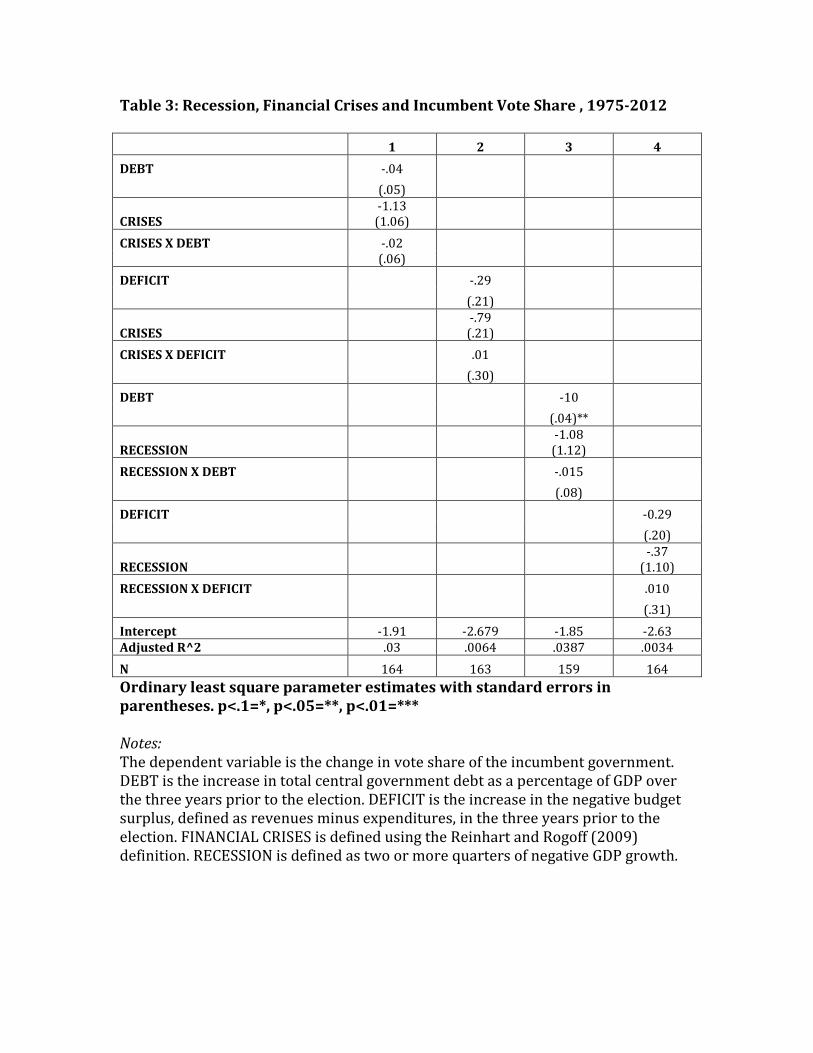
Table 3: Recession, Financial Crises and Incumbent Vote Share , 1975-2012 1 2 3 4 DEBT ­.04

(.05)

CRISES ­1.13 (1.06)

CRISES X DEBT ­.02 (.06) DEFICIT

­.29

(.21)

CRISES ­.79 (.21)

CRISES X DEFICIT

.01

(.30)

DEBT

­10

(.04)**

RECESSION

­1.08 (1.12)

RECESSION X DEBT

­.015

(.08)

DEFICIT

­0.29

(.20)

RECESSION ­.37

(1.10) RECESSION X DEFICIT

.010

(.31) Intercept ­1.91 ­2.679 ­1.85 ­2.63 Adjusted R^2 .03 .0064 .0387 .0034 N 164 163 159 164 Ordinary least square parameter estimates with standard errors in parentheses. p<.1=*, p<.05=**, p<.01=*** Notes: The dependent variable is the change in vote share of the incumbent government. DEBT is the increase in total central government debt as a percentage of GDP over the three years prior to the election. DEFICIT is the increase in the negative budget surplus, defined as revenues minus expenditures, in the three years prior to the election. FINANCIAL CRISES is defined using the Reinhart and Rogoff (2009) definition. RECESSION is defined as two or more quarters of negative GDP growth.

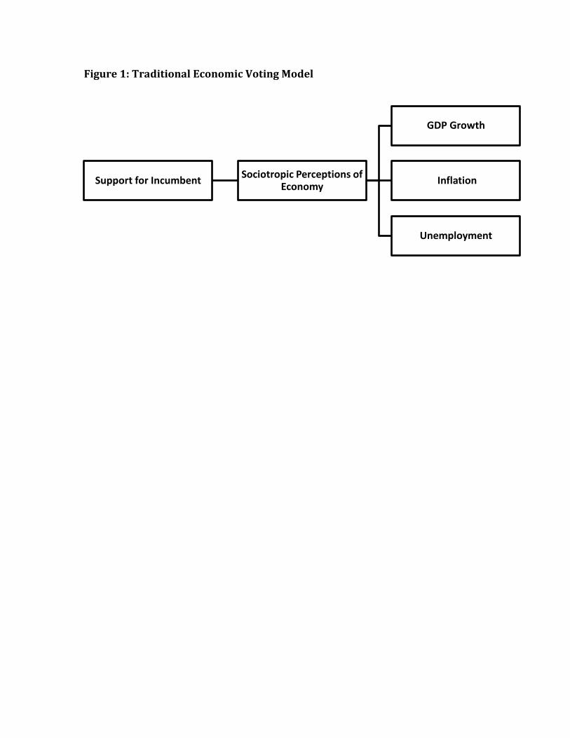
Figure 1: Traditional Economic Voting Model

Support for Incumbent Sociotropic Perceptions of Economy

GDP Growth

Inflation

Unemployment

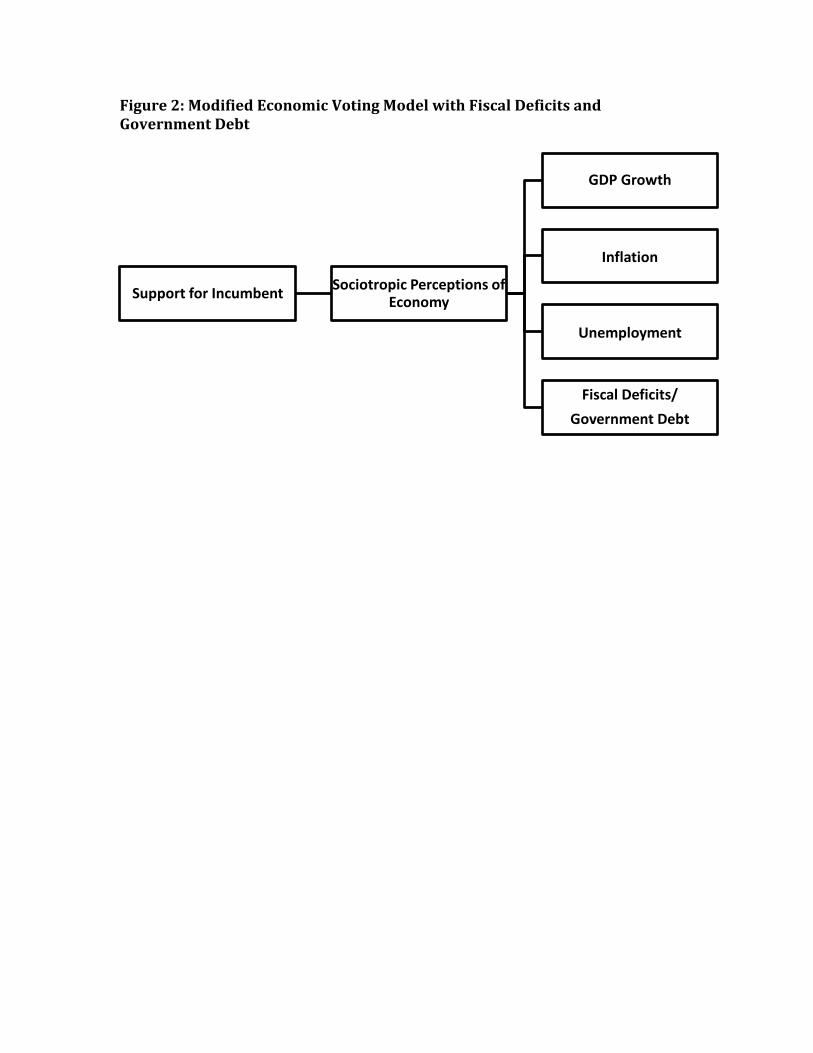
Figure 2: Modified Economic Voting Model with Fiscal Deficits and Government Debt

Support for Incumbent Sociotropic Perceptions of Economy

GDP Growth

Inflation

Unemployment

Fiscal Deficits/ Government Debt

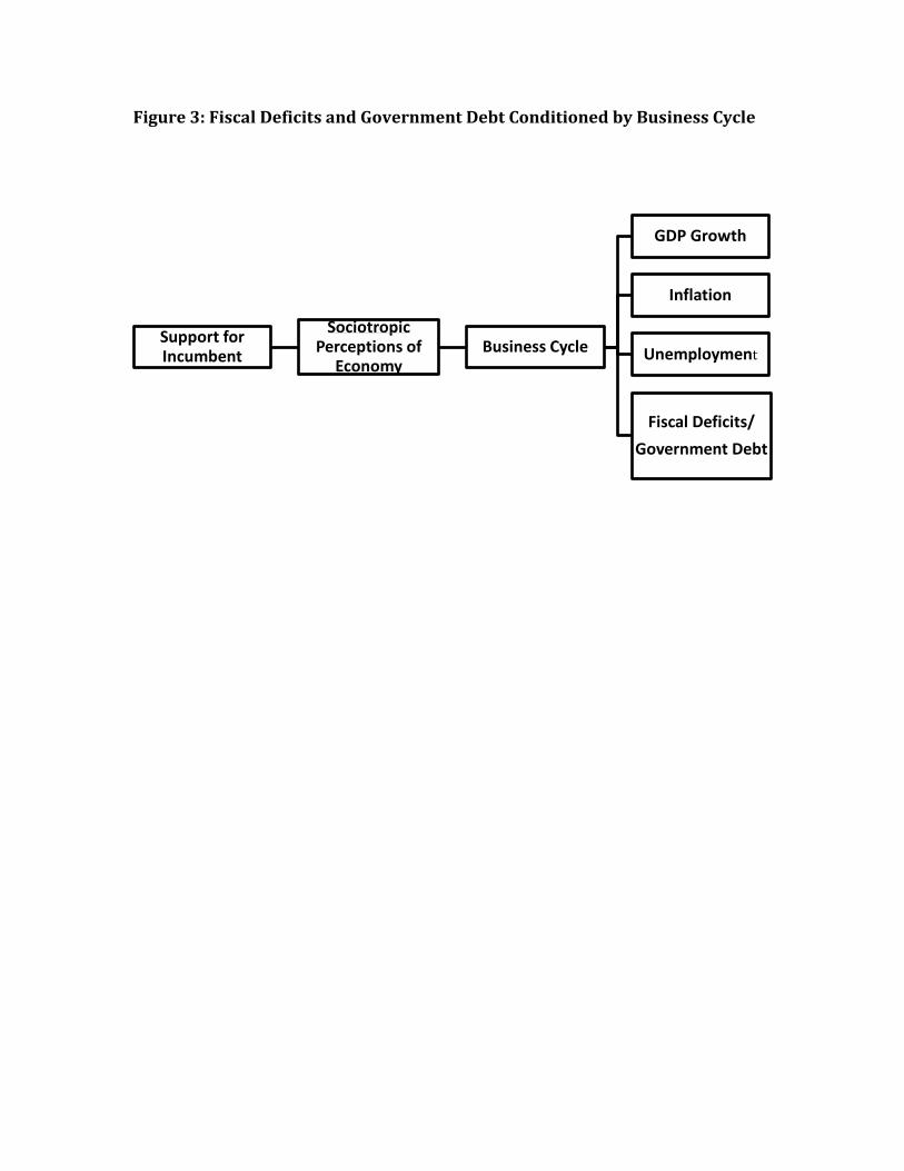
Figure 3: Fiscal Deficits and Government Debt Conditioned by Business Cycle

Support for Incumbent

Sociotropic Perceptions of

Economy Business Cycle

GDP Growth

Inflation

Unemployment

Fiscal Deficits/ Government Debt

Figure 4 Varying Inputs of Fiscal Deficits and Government Debt

Support for Incumbent

Sociotropic Perceptions of

Economy Business Cycle

GDP Growth

Inflation

Unemployment

Fiscal Deficits/ Government

Debt

Stimulus

Bailouts/ Nationalizations

Figure 5: Election Year GDP and Incumbent Vote Share, 2007-2011

EST 07

FIN 07

ISL 07 IRL 07 FRA 07

TUR 07

GRC 07

POL 07

DNK 07

ESP 08 ITA 08

SVN 08

AUS 08

CAN 08

USA 08

NZL 08 ISR 09

ISL 07

JPN 09

NOR 09

DEU 09

PRT 09 GRC 09 CHL 09

HUN 10

GBR 10

NLD 10

SVK 10

AUS 10

SWE 10

USA 10

IRL 11

EST 11

FIN 11

CAN 11

PRT 11

TUR 11 DNK 11

POL 11

ESP 11

NZL 11

SVN 11

­30

­25

­20

­15

­10

­5

0

5

10

15

­10 ­5 0 5 10 15

Chan

ge in

Incu

mbe

nt S

hare

(%)

Change in GDP (% by Quarter)

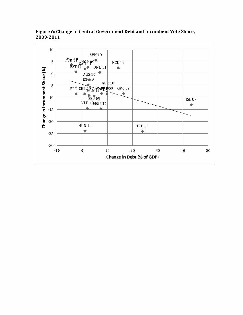
Figure 6: Change in Central Government Debt and Incumbent Vote Share, 2009-2011

ISR 09

ISL 07

JPN 09

NOR 09

DEU 09

PRT 09 GRC 09 CHL 09

HUN 10

GBR 10

NLD 10

SVK 10

AUS 10

SWE 10

USA 10

IRL 11

EST 11

FIN 11

CAN 11

PRT 11

TUR 11

DNK 11

ESP 11

NZL 11

­30

­25

­20

­15

­10

­5

0

5

10

­10 0 10 20 30 40 50

Chan

ge in

Incu

mbe

nt S

hare

(%)

Change in Debt (% of GDP)

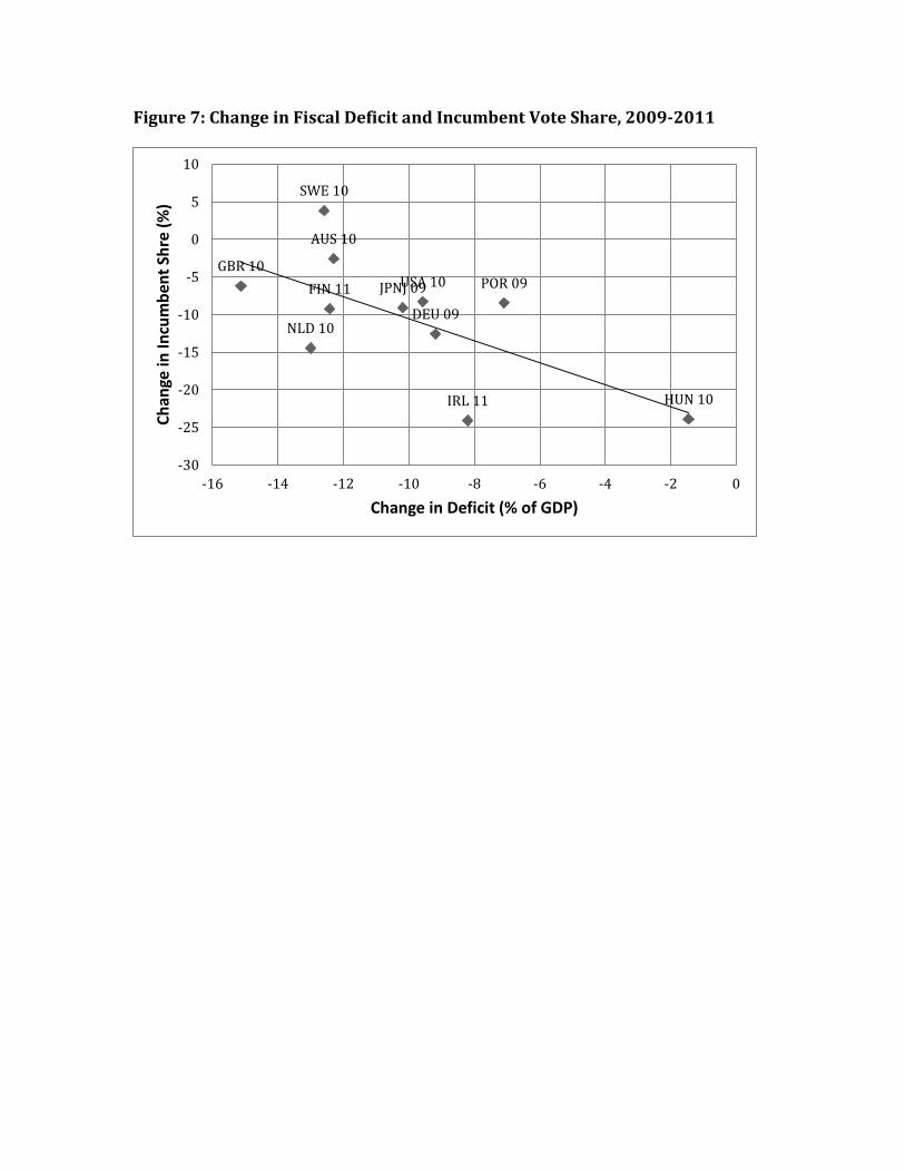
Figure 7: Change in Fiscal Deficit and Incumbent Vote Share, 2009-2011

JPNJ 09

DEU 09

POR 09

HUN 10

GBR 10

NLD 10

AUS 10

SWE 10

USA 10

IRL 11

FIN 11

­30

­25

­20

­15

­10

­5

0

5

10

­16 ­14 ­12 ­10 ­8 ­6 ­4 ­2 0

Chan

ge in

Incu

mbe

nt S

hre

(%)

Change in Deficit (% of GDP)

Figure 8: Election Year GDP Growth and Incumbent Vote Share, 1975-2012

­10

­5

0

5

10

15

­40 ­30 ­20 ­10 0 10 20 30

Chan

ge in

Incu

mbe

nt S

hare

(%)

Change in GDP (% by Quarter)

Figure 9: Change in Gross Government Debt and Incumbent Vote Share , 1975-2012

­40

­30

­20

­10

0

10

20

30

­250 ­200 ­150 ­100 ­50 0 50 100 150

Chan

ge in

Incu

mbe

nt S

hare

(%)

Change in Debt (% of GDP)

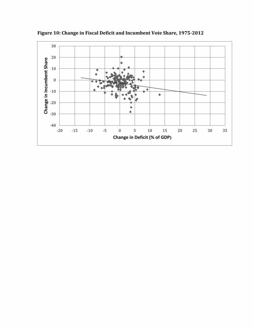
Figure 10: Change in Fiscal Deficit and Incumbent Vote Share, 1975-2012

­40

­30

­20

­10

0

10

20

30

­20 ­15 ­10 ­5 0 5 10 15 20 25 30 35

Chan

ge in

Incu

mbe

nt S

hare

Change in Deficit (% of GDP)