THE KEYNESIAN MODEL OF AGGREGATE DEMANDmcelroy/302/E_Chpt3.pdf · The concept of aggregate demand has four important characteristics: 1. ... Chapter 3 The Keynesian Model of Aggregate

The Macroeconomy—Private Choices, Public Actions, and Aggregate Outcomes

Michael McElroy (©2005)

CHAPTER 3 THE KEYNESIAN MODEL OF AGGREGATE DEMAND 3.1 Introduction

he Classical tradition provided an analysis of the determinants of output in which the supply side (capital, labor, and the institutional structure underlying the production process)

predominated over demand (spending, money supply, and government fiscal actions) in explaining overall economic activity. This was a widely-accepted framework that John Maynard Keynes initially embraced, but came to scorn. His four sentence opening chapter is blunt.

I have called this book the General Theory of Employment, Interest, and Money, placing the emphasis on the prefix general. The object of such a title is to contrast the character of my arguments and conclusions with those of the classical theory of the subject, upon which I was brought up and which dominates the economic thought, both practical and theoretical, of the governing and academic classes of this generation, as it has for a hundred years past. I shall argue that the postulates of the classical theory are applicable to a special case only and not to the general case, the situation which it assumes being a limiting point of the possible positions of equilibrium. Moreover, the characteristics of the special case assumed by the classical theory happen not to be those of the economic society in which we actually live, with the result that its teaching is misleading and disastrous if we attempt to apply it to the facts of experience.1

What so many have believed for so long, asserts Keynes, holds true only under particular circumstances that no longer exist. He claims that the policy implications of this outdated model are destructive when applied to the economic reality of his day.

Keynes was just one of many to attack the Classical view of the overall economy. Why his judgment was so much more influential than the others is a complicated question. Certainly a main factor was its innovative analytical structure -- one that focused on the significance of aggregate demand in the determination of the "wealth of nations". Disciples, opponents, and the undecided vote of his generation generally agreed that, whatever its merits, Keynesian economics was a distinct break from the past. Eventually a sizable majority of economists were joined by opinion-leaders, policy-makers, and the media in proclaiming the "Keynesian Revolution". With more than half a century of hindsight and, especially, with the resurgence of the Classical tradition over the past 30 years, Keynes's work now seems less radical to most economists, less of a break from the Classical path. But it is still a departure and his analytical framework continues to structure our thinking about the macroeconomy.

In the last chapter we saw that aggregate demand was quite unimportant in the Classical system. Only changes in the money supply could alter demand ("only money matters" while "fiscal policy is powerless"), yet even this had no impact on output and employment ("money is

1 John Maynard Keynes, The General Theory of Employment, Interest, and Money, (London: Macmillan Publishing Company, 1936), p.3.

T

Part II Basic Macroeconomic Analysis 2

a veil"), which stay at their full employment levels in equilibrium ("full employment prevails"). With demand playing such a minor role, little attention was paid to its underlying determinants. But as we adjust our focus from the longer run Classical equilibria to short run adjustments, we discover that velocity and therefore aggregate demand is not always the passive, domesticated creature of the Quantity Theory. Hence the Classical model's reliance on constant velocity may no longer offer the best route to understanding the determinants of aggregate demand. This chapter presents the elements of Keynes's alternative approach to the demand side of the macroeconomy, explained within the expository framework developed by another famed British economist, Nobel laureate John Hicks (1904-1989).2 3.2 What is “Aggregate Demand”? Before beginning our search for a theory of aggregate demand, let's make sure we know what we're after. The concept of aggregate demand has four important characteristics:

1. Aggregate demand includes only the demand for "final" goods and services during a certain interval of time, such as a year. Since our focus is on the goods and services that make up our standard of living, we want to be sure to include each relevant item once and only once. This is an obvious point but requires some attention simply because the production process for most products occurs in a series of steps. We want to include the production of automobiles, computers, and bread, but not separately count the intermediate goods (steel, silicon chips, flour) that are already included in final output. By counting demand only at its final stage of production and sale, the value of intermediate products is automatically included and they must not be counted again as separate items.3

2. Aggregate demand represents the demand for final goods and services produced in a particular economy. Aggregate demand for U.S. output must include the demand for our exports by other countries but exclude our demand for their output. The way this is done in practice is to first count all spending by U.S. citizens, businesses, and governments on final goods and services regardless of where they were produced. Then we add in foreign demand for our exports but also subtract that portion of our total spending that went for imports.

2 Hicks' interpretation of The General Theory ("Mr. Keynes and the Classics", Econometrica, 1937) was set in what he labeled the IS-LM model. While this framework is exceedingly useful, it is important to remember that it is incomplete (for example, it only looks at demand, not supply) and even when joined to a model of aggregate supply, makes some simplifications that limit its applicability. Like any approximation to the complex reality of macroeconomic events, it needs to be used carefully.

3 One qualification needs to be made. Total demand for final goods does include one type of "intermediate" output -- investment spending. The value of these new capital goods will eventually show up in the future consumption goods and services that they produce. To avoid double-counting, we deduct a capital consumption allowance (often called depreciation) as this capital is used up and transformed into other final goods and services over the years. Ultimately the original investment expenditure is completely offset by deductions for capital consumption. The net result of putting investment in now and taking it out later is simply to alter the timing of measured output in order to give a more accurate reflection of current economic activity year by year.

Chapter 3 The Keynesian Model of Aggregate Demand 3

This is done through a net exports variable -- exports minus imports, which we denote by the symbol x. To get total demand for U.S. output, then, we add net exports to total spending on consumption, investment, and government output. For the U.S., net exports have been a large negative number for more than a decade.

3. Aggregate demand is measured in monetary units such as dollars or francs or yen. Money represents a common unit of measure that can be applied to such diverse objects as bushels of grain, gallons of milk, and miles of flight. But unlike other units of measure, monetary units change "length" over time because of inflation. As a result, comparisons across the years (for example, comparing the Federal deficit in 1990 with 1980) must be done in constant dollars if they are to have any economic meaning. This requires the use of a price index (basically the average level of prices denoted by P in the previous chapter) to adjust for changes in the unit of measure. It also raises a number of conceptual and practical problems in measurement that are better appreciated after you have a good grasp of the analytical issues. They will be discussed in Chapter Fifteen "Models & Reality".

4. Aggregate demand for final output is the same thing as aggregate income. For the whole economy, every dollar spent on final goods and services must also be a dollar received by someone as income. No unclaimed dollars are left lying around. If we denote total spending and total income as P·yAD and P·y respectively, this says that they are equal and, dividing (deflating) both by P, that real income equals real aggregate demand, y=yAD. In the next chapter we will add the market-clearing condition that aggregate demand and supply must be equal, i.e., yAD = yAS. In anticipation of this, we can makes things simpler by using the symbol "y" to represent all three concepts -- total real income, total real demand, and total real supply of output. Note the adjective "real", reflecting the fact that for now we are correcting for any changes in the price level due to inflation and focusing on the underlying "quantities" of output that determine our economic well-being. In other words, we assume that purely "inflationary" changes in income or spending due to a changing price level have been eliminated.

Having defined aggregate demand, we turn to the harder task of explaining its changes

over time. In other words, we move from a definition to a theory of total demand. Following Keynes, we set aside the quantity theory of money approach to aggregate demand. Instead we formulate four hypotheses about what factors influence planned (or equilibrium) spending: one for each of the four categories of aggregate demand -- consumption (c), investment (i), government (g), and net exports (x).4 Aggregate demand, then, can be written as: 4 What if unanticipated events frustrate our planned levels of spending? For example, unexpectedly poor sales would leave businesses with an unplanned increase in inventories, a capital investment that was not desired. This deviation from the planned or equilibrium level of spending is assumed to lead to revised spending plans for the next year and, barring further unforeseen events, a return to equilibrium or intended levels. Therefore y=c+i+x+g is the equation for the equilibrium level of aggregate demand in the economy. For now we assume that such deviations from equilibrium are relatively small and quickly corrected.


y = c + i + x + g. [Equilibrium Condition] Together, the hypotheses about the four terms on the right hand side will form the basis of a model of equilibrium aggregate demand that is more powerful than the Classical demand theory of the previous chapter but also more complex. To keep it from getting too complicated, too quickly, let's start with the simplifying assumption that three of the four components of total demand are constant. We'll focus on consumption spending (c) as we pretend that spending on investment, net exports, and government is fixed at the values i0, x0, and g0, respectively. This pretense of constancy is dropped in just a few pages. 3.3 The Consumption Function

multitude of factors influence total consumption demand for the whole economy in a given year. To avoid becoming mired in details, we note that spending on current consumption is

limited by our available purchasing power which, in turn, depends upon our lifetime income stream -- our past, present, and future income. Past income can influence current consumption through accumulated savings (net worth) while future income can be used to the extent that we can borrow on it, consuming now and paying back later.

As important as past or future earnings might be in determining our current consumption spending, the Keynesian explanation of consumption puts the emphasis only on the role of our present after-tax earnings, sometimes called "current disposable income". In a later chapter we will build upon this lifetime view in which saving and borrowing, via capital markets, combine to moderate the influence of current economic events and policies on consumption spending. For now, though, we follow Keynes and emphasize the connection between current consumption (c) and current after-tax income (y-t), in what he termed the consumption function: c = c0 + c1(y-t) , [Consumption Function] where c0>0 and 0<c1<1. The c0 and c1 terms are called coefficients or parameters and are symbols that represent particular numerical values.5

Like all equations, the consumption function is a sentence, expressed in the compact language of algebra. It emphasizes the relationship between current consumption and current after-tax income and their linkage through the parameter c1, called the marginal propensity to consume. Other determinants of current consumption spending -- past income, future income, and everything else -- are all lumped together in the c0 term. This is called autonomous consumption, "autonomous" in the sense that it stands by itself, independent of the influence of after-tax income. Keeping the focus on the short run for now, we assume that c0 and c1 are both constant so that the sole determinant of changes in current consumption spending is changes in current after-tax income.

To get an idea of the workings of the consumption function, note that if after-tax real

5 Specific values of c0 and c1 can be estimated from past data using techniques such as least squares regression. This process of converting our economic models into econometric models is discussed in Chapter 15.

A


income increases, real consumption will increase by the fraction c1 times ∆(y-t).6 The remainder of that increase in income, the fraction (1-c1)∆(y-t), is defined as current real saving and denoted by the symbol s. For example, if the marginal propensity to consume (c1) is .9 and after-tax income rises by $100, then the change in consumption is given by ∆c=c1∆(y-t)=.9($100)=$90. A $100 increase in current disposable income causes current consumption to rise by $90. The remaining $10 [(1-c1)∆(y-t)=(1-.9)100=.1(100)] goes into current saving, making it available for future consumption. A lower value of c1 would describe a weaker link between current consumption and current income, so that a smaller share of any increase in after-tax income would go into current consumption but a larger share into current saving.7

IN SUMMARY . . .

The Consumption Function Current consumption demand depends on many factors, particularly current income (after taxes) as well as savings from the past and borrowing on the future. The Keynesian consumption function, c=c0+c1(y-t), captures four important characteristics:

1. Current consumption changes in the same direction as current after-tax income but not by as much since the two are connected by the fraction c1. 2. Because consumption is assumed to depend on after-tax income (y-t), it responds identically to either a change in income (∆y) or a change in taxes (∆t). 3. The part of any change in after-tax income that does not go into consumption is added to current saving. That is, ∆s = (1-c1)∆(y-t), where (1-c1) is the fraction of after-tax income that is saved. 4. All determinants of consumption other than after-tax income are grouped together in the autonomous consumption term, c0.

6 Since c=c0+c1(y-t), then a change in after-tax income [∆(y-t)] must alter both sides of the equation. We can write this as: c+∆c=c0+c1[(y-t)+ ∆(y-t)]. Multiplying out and canceling leaves us with ∆c=c1∆(y-t). Put another way, the first derivative of consumption with respect to after-tax income is equal to c1, i.e. dc/d(y-t)=c1.

7 By convention, "saving" is the part of current income that we set aside, whereas the plural "savings" refers to accumulated saving over the years, e.g., from past saving. Saving in any particular year can, of course, be negative if we consume more than our current income by drawing on past saving or borrowing from future income.


3.4 The “Multiplier” Process

e have seen that the equilibrium aggregate demand equation is y=c+i+x+g. This tells us that current income depends, in part, on current consumption spending (+∆c ═> ∆y) while

the consumption function, c=c0+c1(y-t), says that current consumption spending depends, in part, on current income (+∆y ═> +∆c). This two-way interaction between consumption and income probably seems pretty obvious and you may wonder why we have to substitute equations for ordinary common sense. The reason is one that will become increasingly apparent as we begin to make the analysis more realistic: When there are two or more interdependent events, understanding their cumulative effects can quickly exceed the important but quite limited powers of "common sense".

To see the significance of this mutual causality between consumption and income, suppose government spending is increased and we want to predict what affect this will have on aggregate demand (y). Continuing the simplifying assumption that investment, net exports, government spending, and taxes are known and constant, we have the following information about aggregate demand: y = c + i + x + g (1) Equilibrium condition c = c0 + c1(y-t) (2) Consumption Function t = t0 (3) Taxes i = i0 (4) Investment Demand x = x0 (5) Net Export Demand g = g0 (6) Government Demand This is a six equation model or, equivalently, a six sentence "story" about what determines the level of aggregate demand. Our focus is on the interaction between the first two equations, keeping the other four "constants" in the background for the moment.

A given increase in government spending (+∆g) will cause total demand to rise by the same amount (+∆y=+∆g), according to equation 1. But the consumption function tells us that this increase in income raises after-tax income and thereby increases consumption spending by a fraction (c1) of the increased income, i.e., ∆c=c1∆(y-t). It is at this point that the feedback begins as the increased consumption spending causes another increase in income (+∆y'=+∆c=c1∆(y-t)) raises income a second time. This boost in disposable income will, in turn, increase consumption again, then income, then consumption and so on as the first two equations reinforce one another through what is aptly called the multiplier process.

The "multiplier" might be likened to a game of tag or a cat chasing its tail. Alternatively, we could emphasize its cumulative potential and portray it as an avalanche or even a nuclear chain reaction. Which, if any, of these images describes the final economic impact of the increase in government spending on aggregate demand? To see which pattern, which metaphor, we're dealing with here let's return to the primary metaphor in economics—algebra. Remember that metaphor works by treating an unfamiliar "this" as if it's a more familiar "that". Using the operations of algebra as an analog ("that") for economic events ("this"), we solve this model of total demand by substituting the last five equations into the first.

W


y = c + i + x + g (1) c = c0 + c1(y-t) (2) t = t0 (3) i = i0 (4) x = x0 (5) g = g0 (6) Substituting and solving for aggregate demand/income:

y = c0 + c1(y-t0) + i0 + x0 + g0 y = c0 + c1y - c1t0 + i0 + x0 + g0 y - c1y = c0 - c1t0 + i0 + x0 + g0 (1-c1)y = c0 - c1t0 + i0 + x0 + g0

y = [1/(1-c1)] (c0 - c1t0 + i0 + x0 + g0) More concisely, we can write the solution for y as: y = µ0(z0 + g0 - c1t0) , [Solution (IS) Equation] where µ0 = 1/(1-c1) and z0 = c0+i0+x0.

This solution equation condenses all the information from the six sentence "story" of aggregate demand into a single "sentence". It's traditionally called the IS Equation, following the original derivation by John Hicks (1937) which used an equivalent framework that started from investment and saving, hence I and S. The text box below shows the solution in numerical terms to reinforce the basic mechanics of this model.


Solving the Six-Equation Demand Model: NUMERICAL SOLUTION

Suppose a statistical study reveals that aggregate consumption for the whole nation can be reliably, if not exactly, predicted as $10 billion plus 90% of current after-tax income. Also assume we can make good guesses at this year's level of tax revenues ($80 billion), investment spending ($30 billion), government spending ($80 billion), and net exports ($-8 billion). Incorporating this information into our model of aggregate demand, we solve for the equilibrium values of income and consumption.

y = c + i + x + g (1) c = 10 + .9(y-t) (2) t = 80 (3) i = 30 (4) x = -8 (5) g = 80 (6)

Substituting into the first equation yields,

y = 10 + .9(y-80) + 30 – 8 +80 y = 112 + .9y – 72 .1y = 40 y = 400

This says that the only value of total demand (y) that satisfies all six equations is 400. We can then solve for the value of consumption by substituting into the second equation:

c = 10+.9(y-t) c = 10+.9(400-80) c = 298


Let's now use these equations to get at the multiplier process through which an initial increase in government spending touches off a series of interactions between consumption and income. Starting with the numerical values given in the text box, suppose there's an increase in government spending from $80 to $100 billion. What happens to the level of aggregate demand/income? Because of the interdependence embodied in the first two equations, the rise in government spending triggers a sequence of events in which the initial +∆g=20 increases demand by 20, with 18 (.9 of 20) going into consumption and the remaining 2 (.1 of 20) to saving. This increase in consumption spending means another increase in income, this time by 18 which in turn will increase saving by 1.8 (.1 of 18), with the remaining 16.2 (.9 of 18) going to consumption. This increased consumption spending then increases income by another 16.2, which causes consumption to rise by 14.58 (.9 of 16.2) and on and on. The sum total of all the increases in spending/income (the +∆y's) will be the initial 20 plus a succession of increments that are each 90% (the part of income that goes into consumption) of the previous change: 20 + .9(20) + .9(.9)(20) + (.9)(.9)(.9)(20) + . . . = 20 + 18 + 16.2 + 14.58 + . . . and so on.

The obvious question is how to get to the end of this sequence of interactions in order to determine the size of the multiplier effect. This is where some basic algebraic results can be a welcome companion to common sense. Continuing the numerical example, let's solve the six equations together again, but this time with g=100 rather than the initial 80. The result is:

y = 10 + .9(y-80) + 30 - 8 + 100 y = 132 + .9y – 72 .1y = 60 y = 600

When government spending was 80 we found that total demand was 400. So the increase in government spending from 80 to 100 (+∆g=20) has increased total income from 400 to 600 (+∆y=200). So the cumulative effect of all those increments (20+18+16.2+. . .) turns out to be 600-400=200. In other words, the initial change was magnified ten-fold through the consumption/income interaction of the multiplier, telling us that the value of the multiplier is ∆y/∆g=200/20=10.

Referring back to our earlier list of potential metaphors for the multiplier process, it did not explode to infinity or chase its own tail forever. Instead, the size of the consumption/income interaction gradually dwindled away but left behind a sizable cumulative jump in the overall level of demand. A $20 billion increase in government spending set off a series of events that eventually increased aggregate demand from $400 to $600 billion, a ten-fold increase in the initial spending change.

The basic idea of the multiplier process should now be clear. The consumption/income

interaction magnifies a given increase in spending because that spending becomes someone's income, a fraction of which becomes new spending which in turn generates more income and so on. This was illustrated with a numerical example, followed by the general result that the size of the multiplier depends on the "marginal propensity to consume", the fraction (c1) of a change in after-tax income that goes into consumption spending. We saw that for c1=.9, the size of the multiplier was 10. But if the marginal propensity to consume dropped to c1=.8, the multiplier would decline to µ0=1/(1-c1)=5. If we consumed only half of any increment to our income, this c1=.5 would yield a multiplier of 2. As a smaller fraction of a change in our income


goes into consumption (hence more into saving) the consumption/income interaction is diminished and the multiplier reduced in size. We've derived the multiplier in response to a specific question—What impact will an increase in government spending have on total income/spending in our six equation model of aggregate demand? But the multiplier concept can be applied far beyond this particular example. Returning to the algebra (but remembering that it's just a tool for establishing economic results), let's look at three further implications of the multiplier.

▪ THE MULTIPLIER WORKS IN BOTH DIRECTIONS

The multiplier equation ∆y=µ0∆g0 makes no distinction between an increase and a decrease in government spending. This algebraic symmetry has a potentially very significant implication when applied to the macroeconomy. A cut in government spending, for example, will decrease total spending/income by a

A SHORT CUT TO THE MULTIPLIER

To determine that the multiplier in our example was 10 we had to solve the model twice, once with g=80 and then with g=100. Then we compared the resulting change in total spending/income (∆y) to the initial change in government spending (∆g). Fortunately there's a much simpler way to find the size of the multiplier that doesn't require us to solve and then re-solve the entire six equation model.

Remember that the general solution is given by the IS equation, y = µ0(z0 + g0 - c1t0), where µ0 = 1/(1-c1) and z0 = c0+i0+x0. To see what happens to equilibrium income when government spending changes, we can just add ∆g0 to the original g0 on the right hand side, knowing that the left hand side will then change by some amount ∆y. Therefore,

y + ∆y = µ0[z0 + (g0+∆g0) - c1t0], or y + ∆y = µ0(z0 + g0 - c1t0) + µ0∆g0 , and canceling gives ∆y = µ0∆g0 [Multiplier Equation] hence, ∆y/∆g0 = µ0. [Spending Multiplier]

What have we discovered here? Without using any specific numbers, we have derived a useful general result: When government spending changes, the equilibrium value of income will change by the amount µ0∆g0. Since µ0=1/(1-c1) and 0<c1<1, then µ0 must take a value greater than one and it represents the value of the demand-side spending multiplier.

Therefore we need know only the value of c1 to determine the impact of a given change in government spending on total spending/income. Applied to our numerical example, the initial $20 billion increase in spending will ultimately increase total demand by

∆y = µ0(∆g0) = [1/(1-c1)](∆g0) = [1/(1-.9)](20) ∆y = (1/.1)(20) = 10(20) ∆y = 200

Chapter 3 The Keynesian Model of Aggregate Demand11

multiple of the initial change in demand. If, as Keynes believed, this drop in total demand causes a short run decline in real output, then this model may be able to identify the causes and cures for periods of economic recession.

▪ ANY CHANGE IN SPENDING WILL SET OFF THE MULTIPLIER PROCESS

In our example the interaction between consumption and income was initiated by a change in government spending. But it could just as well have been a change in any of the components of autonomous private spending, i.e., ∆c0, ∆i0, or ∆x0. To see this, we return to the solution of the six-equation model of demand, shown in the IS equation.

y = µ0(z0 + g0 - c1t0) [Solution (IS) Equation]

We previously derived the multiplier by asking what would happen to total spending (y) if we increased government spending by the amount ∆g0. Now let's ask what happens if there's a change in any of the three components of autonomous private spending (z0=c0+i0+x0). We simply repeat the process of adding in something (this time ∆z0) on the right hand side of the IS equation, then solving for the value of the balancing ∆y on the left hand side.

y + ∆y = µ0[(z0+∆z0) + g0 - c1t0] y + ∆y = µ0(z0 + g0 - c1t0) + µ0∆z0 , and canceling gives ∆y= µ0∆z0, where m0 = 1/(1-c1) & z0=c0+i0+x0.

This tells us that the multiplier applies to any change in aggregate demand, public (g) or private (c+i+x). It also raises the possibility of a countercyclical increase in government spending (+∆g0) to offset the economy-wide consequences of a drop in private demand (-∆z0). Remember that the potential for countercyclical fiscal actions never arose in the Classical model where aggregate demand was determined entirely by the money supply and the presumably constant velocity of money.

▪ TAX CHANGES ALSO HAVE A MULTIPLIER EFFECT ON TOTAL DEMAND

The consumption function (c=c0+c1(y-t)) assumes that changes in taxes alter after-tax income and hence consumption. Since this change in consumption also affects income (y=c+i+x+g), it also triggers a multiplier process. The algebra of this is again straightforward. In the solution equation (IS) we now ask what happens to total demand (y) if we change the level of taxes (t0).

y = µ0(z0 + g0 - c1t0), [Solution (IS) Equation]

Adding the amount ∆t0 to the initial level of taxes and balancing it with ∆y,

y + ∆y = µ0[z0 + g0 - c1(t0+∆t0)],


we then multiply through and cancel to get

y + ∆y = µ0(z0 + g0 - c1t0) - µ0c1∆t0 ,

∆y = -c1µ0∆t0 and [Tax Multiplier Equation] ∆y/∆t0 =-c1µ0. [Tax Multiplier]

Routine algebra, unexciting at best, has revealed an important result that would otherwise be hard to spot. The tax multiplier (∆y/∆t0=-c1µ0) turns out to be a fraction (c1) of the expenditure multiplier (µ0) and works in the opposite direction. For example, if c1=.9 so that the expenditure multiplier (µ0) was 10, then a $10 billion increase in public or private spending (∆g0 or ∆z0) will increase total demand by $100 billion. In contrast, a $10 billion increase in taxes will lead to a $90 billion drop in demand. The higher taxes reduce consumption and set off a downward multiplier process. But the total effect is smaller in absolute value ($90 rather than $100) because only a fraction (c1) of the initial tax change goes into spending changes.

A word of caution is appropriate here. The discovery of a tax-multiplier lurking inside our model is correct and important. But don't forget that this is a quite simple, uncomplicated model compared with the reality it describes. In later chapters we'll see some good reasons to suspect that this model over-estimates, perhaps greatly, the power of current tax changes to affect aggregate demand.8

3.5 Refining the Multiplier

he multiplier process exists because a fraction of any increase in after-tax income is spent on consumption which, in turn, increases income and so on in an interplay of forces

between the first two equations in the demand model. The larger the marginal propensity to consume (c1), the larger the multiplier. An increase in income in our model either goes into consumption, feeding the multiplier process, or it exits the "spending stream" and implicitly goes into saving. Saving, then, can be thought of as a "leakage" from the current flow of spending. The smaller the marginal propensity to consume, the larger this leakage and hence the smaller the multiplier.

In reality there are other important leakages from the spending stream and the failure to include them results in a significant overestimate of the size of the multiplier. Like saving, they reduce the fraction of an increase in income that goes into current consumption (of domestic goods) and thereby lower the size of the multiplier. Two of these additional leakages are

8 As a preview, remember from Chapter 1 that lowering taxes now simply means higher taxes later, assuming government spending is unchanged. If such a tax "cut" is viewed as just a tax postponement, people may not increase current consumption very much, if at all. Put another way, a cut in current taxes would stimulate consumption only if people were economically "nearsighted" and ignored the fact that a tax cut now must be paid back later plus interest.

T


particularly significant -- income taxes and imports.

We saw that each round of the multiplier adds an increment to income. Taxes (t0) were assumed to be given and unchanging. So changes in income through the multiplier didn't alter the amount of taxes. In the "real world", the existence of an income tax means that each part of each round of the multiplier is diverted to taxes and therefore is a leakage from the consumption/income dynamics of the multiplier process. We incorporate this into our analysis by rewriting the tax equation as:

t = t0 + t1y , [Tax Function] where t0>0 and 0<t1<1. As before, t represents this year's total tax revenues, but is now divided into two parts. The t0 term represents the level of all non-income taxes, such as sales and property taxes. The t1y term shows the amount of revenue generated by the income tax, since y is before-tax total income and t1 is the income tax rate.9

As the above tax function reveals, an increase in income raises tax revenues by t1∆y. For example, if the income tax rate is 20% (t1=.20), then an increase in income of $2000 will create $400 in additional taxes, leaving $1600, rather than $2000, to be split between saving and consumption. As each increment in consumption creates another increase in income, 20% will be siphoned off the top for taxes, reducing the multiplier accordingly.

In addition to generating taxes, an increase in income also results in more consumption of both domestic and imported goods. Since this last part is not a demand for U.S. output, it represents another leakage from the U.S. expenditure stream. It shows up in the first equation (y=c+i+x+g) as a reduction in net exports (-∆x). We can express this inverse relationship between net exports and income by expanding the net export equation as follows:

x = x0 - x1y , [Net Export Function]

where x0 can take any sign and 0<x1<1.

So x represents net export demand (exports minus imports), x1 (sometimes called the "marginal propensity to import") is the fraction of an increase in our income that is spent on other countries' products, and x0 ("autonomous" net exports) represents everything that influences net export spending other than current income. This equation shows that an increase in income reduces net exports, causing a further leakage from spending on U.S. goods of the amount x1∆y.

How can we adjust our multiplier to include these two additional leakages from the

spending stream? Intuitively, the situation is not hard to understand. The interaction between changes in consumption and changes in income that comprises the multiplier is now diminished

9 This equation embodies a constant income tax rate, called a proportional income tax. A progressive income tax system, in which the tax rate rises with the income level, is more realistic but also more complicated to handle. We keep the simpler assumption because it yields virtually the same analytical and policy conclusions.


by leakages out of domestic consumption due to saving, income taxes, and imports. It takes only a little more work to find the actual size of this new multiplier. Adding the revised tax and net export equations into the six equations gives us the following more realistic model of the demand for output, y.

y = c + i + x + g (1) c = c0 + c1(y-t) (2) t = t0 + t1y (3)* i = i0 (4) x = x0 - x1y (5)* g = g0 (6)

Again taking advantage of the relative simplicity of algebra (compared to handling all

these interactions in words), we substitute the last five equations into the first and solve for total demand/income (y). y = c0 + c1[y-(t0+t1y)] + i0 + x0 - x1y + g0 y = c0 + c1y - c1t0 - c1t1y + i0 + x0 - x1y + g0 y-c1y+c1t1y+x1y = c0 - c1t0 + i0 + x0 + g0 y(1-c1+c1t1+x1) = c0 - c1t0 + i0 + x0 + g0 y =[1/ (1-c1+c1t1+x1)](c0 - c1t0 + i0 + x0 + g0)

and, more concisely,

y=µ(z0+g0-c1t0) , [Solution (IS) Equation]

where we still have z0=c0+i0+x0, as before, but the multiplier is now µ=1/(1-c1+c1t1+x1).

This is the solution of a more realistic model of aggregate demand, incorporating the dependence of taxes and net exports on the level of income. We have again condensed a six sentence story about aggregate demand into a single sentence. In other words, we have derived a new IS equation that incorporates a more complete and realistic treatment of taxes and imports.

Notice that the only difference between this new solution and the earlier one is that we

now have µ rather than µ0 for the multiplier term. How do they differ? Intuitively, we know that since two additional leakages have been added, the new multiplier must be smaller. A look at the algebra confirms this, since µ=1/(1-c1+c1t1+x1) has a larger denominator than µ0=1/(1-c1), thereby reducing its size.10 To get an idea of how significant the inclusion of tax and import leakages can be in the multiplier process, let's put in some numbers. Recall that when c1=.9, the earlier multiplier was 1/(1-.9)=10. But if t1=.25 and x1=.075, we now find a substantially reduced multiplier effect with µ=2.5.

10 If t1=x1=0 the two multipliers would be identical, which means that µ0 is a "special case" of the more general, more inclusive µ.


3.6 Some Words of Encouragement

o you have the unpleasant feeling that what looked like it might be an interesting and useful subject is rapidly losing its appeal? This is the point at which the common "economics is

too abstract, too theoretical" syndrome usually sets in. It looks like we've lost sight of the real world and the real issues that involve the lives of real people. We haven't, but for the moment you may need to take it on faith that this tedious algebraic discussion will turn out to be both important and practical. Part of the problem is simply that algebra is not a popular language in which to tell a story. But when the story is a complex one with lots of interrelationships, ordinary language will often tell it badly. For example, explaining the multiplier process in words could give us pages and pages of:

If government spending rises, this increases equilibrium income since every dollar spent is also a dollar received by someone else. This leads, in turn, to an increase in people's planned consumption spending, although not all the increase in income goes into consumption since some is put away for a rainy day as saving. Moreover, some of that increase in income is scooped off the top by Uncle Sam, while still another part of it is spent by consumers on foreign goods which, of course, is not received as income in the U.S. (But don't forget, of course, that foreign spending on our goods is received as income here.) The original increase in government spending, while over and done with now, continues to be felt because it has increased income which in turn increased consumption (after taking out some for taxes, saving, and imports), and it is precisely this

IN SUMMARY . . . THE MULTIPLIER PROCESS The multiplier reflects a two-way interaction between changes in income and changes in consumption. They feed one another, magnifying the overall impact of any change in aggregate demand on the economy. The ultimate size of this magnification depends on the size of the leakages from the spending stream that occur with each round of increased income—increased saving, higher tax payments, and more purchases of foreign goods and services. Specifically, the size of the multiplier is given by µ=1/(1-c1+c1t1+x1). It's impact on total spending/income is captured in the expression y=µ(z0+g0-c1t0), in which any change in private or public spending (∆z0 or ∆g0, respectively) is multiplied by µ and any change in taxes is multiplied by -c1µ. The main implications of the multiplier for the macroeconomy are:

1. The multiplier applies to both increases and decreases in any component of (z0+g0-c1t0). 2. The same multiplier applies to both public and private changes in demand, i.e., ∆y=µ∆g0 and ∆y=µ∆z0. 3. Tax changes have an indirect and partial effect on spending (via consumption) so the multiplier is smaller by the amount c1, i.e., ∆y=-c1µ∆t0. Since higher taxes reduce after-tax income, the tax multiplier has the opposite sign of the expenditure multiplier.

D


increase in consumption which is now received as income by someone else. And out of this new round of income, part will go into saving, taxes, and imports, the remainder going to consumption spending which will increase income yet again and where this process all ends up is a bit hard to tell because basically it just keeps happening over and over, though each time it's a little smaller and so . . .

So many words; so little information. All this has barely scratched the surface. For example, it tells us nothing about the magnitude of the multiplier process. Is it moderate, small, huge, or trivial?

Trying to push the analysis further would only add to the ambiguity and confusion and we would soon abandon it. Where could we turn? Most likely to some combination of political slogans and relatively primitive common sense. But there's always tea leaves and astrological signs for variety. Alternatively, we might try to clarify things by first defining short-hand symbols for the key concepts (e.g., y, c, i, etc.) and then trying to figure out the relationships among them. This response (symbols and their relationships) is exactly what our six-equation model does and the solution equation [y=µ(z0+g0-c1t0)] is exactly the "bottom line" we seek. Ordinary language, rich and powerful in so many ways, is simply inadequate in situations of the "net-result-of-numerous-interactions" type. Interdependence and interaction characterize most of the important issues in macroeconomics and therefore complicate decision-making at all levels—individual, business, and government. Without a little basic algebra to guide us, we're likely to end up making drastic over-simplifications that limit and distort our understanding.

You don't have to be a natural-born mathematician to be a good analyst and problem-solver. High school algebra and geometry plus a little patience are all that's required. If you find this process tedious and distasteful, it may help to remind yourself that we're using mathematics as our metaphor only because it can give relatively clear, easy, and reliable answers to some difficult and very important questions. Yes, we're involved in mathematical operations on abstract symbols, but only superficially. Underneath are the real issues of prosperity and recession, unemployment and inflation, and our hopes for improving our lives through thoughtful individual decisions and public policy-making. Mathematics is a powerful and practical means toward attaining these important ends. 3.7 Extending the Model of Aggregate Demand

emember that we're exploring the determinants of aggregate demand for two reasons: (1) the "quantity theory" approach of the Classical model is limited by the assumption of

constant velocity of money and (2) we want to pursue Keynes's suspicions that changes in aggregate demand cause short run fluctuations in real output and employment. So far we've focused on the multiplier process, the two-way consumption/income interaction moderated by leakages into savings, taxes, and imports. The next step toward a practical understanding of demand is to add the influence of the real interest rate on two of the components of aggregate demand -- investment and net exports.

As with consumption earlier, many factors influence investment demand for the whole economy in a given year. Because spending on a capital good depends not only on the purchase price of these goods but also on the anticipated future returns over their lifetime,

R


changing expectations about future events can have a decisive impact on the level of investment spending undertaken today. This sensitivity to changing expectations makes investment a much more volatile category than consumption. It also makes it more difficult for us to devise a good explanation of investment spending based on currently observable variables. A useful place to start, however, is with the impact of the real rate of interest (r) on current investment spending.11

Investment projects, by definition, yield a stream of returns over time. They are often financed by borrowed funds, which essentially spreads the cost of the new capital over its anticipated economic lifetime. An increase in the real interest rate makes it more expensive to borrow, raising the cost stream and thereby lowering the expected net return on investment spending. Projects that would have been undertaken with a real interest rate of 5%, may be rejected at 7%. Hence there is an inverse relationship between current investment spending and the real rate of interest.

Even if investment is financed through a firm's retained earnings (current saving) rather

than by borrowing, the inverse relationship between the real rate of interest (r) and investment spending (i) remains. The reason is that a rise in interest rates in the economy increases the return a firm could get if it used its retained earnings outside the company to purchase, for example, government bonds. So an increase in the real interest rate increases either the cost of borrowed funds or the opportunity cost of internal funds, thereby making a given investment project more expensive and lowering its expected profitability.

We focus on this connection between investment spending and the real rate of interest by putting all other factors that could influence investment in the "autonomous investment" category (i0). We then have a net real investment function,

i = i0 - i2r , [Investment Equation] where i2>0. Autonomous investment can have any sign, which means that total net investment (i) can be

11 The real rate of interest (r) is an average of the various interest rates in the capital market, adjusted for anticipated inflation. In later chapters, we will discuss both the aggregation issue (using a single number to represent all interest rates) and the important distinction between the real rate (r) and the money or market rate of interest (R).


positive, negative, or zero.12 Both i0 and i2 are parameters of the investment function and can be estimated statistically. The parameter i2 shows the sensitivity of investment to changes in the real rate of interest, i.e. ∆i=-i2∆r.13 A large value of i2 would describe an economy in which a small change in interest rates sets off a relatively large change in investment spending.

12 Zero net investment means that the economy is investing only enough to replace existing capital as it depreciates. So i>0 represents positive net capital accumulation (+∆k, the key ingredient in economic growth and outward shifts in the PPF). An economy with negative net investment (i<0) is "consuming its capital" (-∆k) and its shrinking capital stock means economic decline as shown by a contraction of the PPF.

13Since i=i0-i2r, then a change in the real rate of interest must alter both sides of the equation. We can write this as: i+∆i=i0-i2(r+∆r). Multiplying out and canceling, we get ∆i=-i2∆r. Thus the value of i2=-∆i/∆r represents the responsiveness (or first derivative) of net investment to a change in the real interest rate.

The good news is that adding this new investment equation to our model of demand doesn't involve anything near as complicated as the multiplier interactions we've just done. The bad news is that it has introduced a new variable, the real rate of interest, whose level must be known before we can determine the value of investment and, hence, real output. Put a different way, by trying to make the story more realistic we have introduced an important, but largely unknown character named r. Later in the chapter we'll add information that will clarify the identity of this mysterious stranger and help us bring the basic story of "What determines aggregate demand?" to a conclusion.

But changes in the real rate of interest alter aggregate demand not only through investment spending but also through the net export term. We saw earlier that imports represent a leakage from the spending stream that reduces the size of the multiplier. We must add to this the fact that both exports and imports are also altered by changes in the real rate of interest. This relationship will be discussed carefully in a later chapter. For now we'll just assert that a rise in the real rate of interest results in an increased demand for the U.S. dollar by foreigners looking for a good return on their savings. This increase in the demand for the dollar then pushes up its international value. The stronger dollar now buys more foreign currency, making imports less expensive to U.S. consumers and raising the price of our exports to foreigners whose currency has lost value relative to the dollar. The end result, which is all you need to know for now, is that a rise in the real rate of interest, via events in the foreign exchange market, leads to a reduction in net exports.

This expanded view of net exports is summarized in the following net export demand

function:

x = x0 - x1y - x2r. [Net Exports Equation] where x1,x2> 0.


All factors that might affect net exports other than income and the real interest rate, such as tariffs, are combined into the autonomous net exports term, x0. The size of the parameters x1 and x2 show, respectively, the magnitude of the impact of changes in income and changes in the real interest rate on net exports. The actual size of these coefficients—x0, x1, and x2—can be estimated statistically. 3.8 Implications of the “IS” Model of Aggregate Demand

his chapter has developed a model of aggregate demand in three stages:

1. We started with a simple framework (the six-equation model of demand) that focused on the consumption-income interaction (+∆y<═>∆c) underlying the multiplier process. We discovered an expenditure multiplier of µ0=1/(1-c1) where c1 is the marginal propensity to consume. The tax multiplier was -c1µ0. (Section 3.4 "The Multiplier Process".) 2. We then modified this model in which saving was the only "leakage" from the spending stream, to include leakages to taxes and imports. Adding the dependence of taxes and net exports on income (+∆y ═> +∆t & -∆x) reduced the size of the multiplier to µ=1/(1-c1+c1t1+x1)<µ0. (Section 3.5 "Refining the Multiplier".) This is the multiplier relationship that we'll use throughout the book.

3. We took another step toward realism by adding another important determinant of aggregate demand -- the real rate of interest. Specifically, we added the observed inverse relationship between the real interest rate and both investment and net exports (+∆r ═> -∆i & -∆x). (Section 3.7 "Extending the Model of Aggregate Demand".)

Let's now put these modifications together and explore some of the policy implications of

this expanded model of aggregate demand. As usual, there's too much happening to rely solely on ordinary language so we turn to algebra for assistance. y = c + i + x + g (1) c = c0 + c1(y-t) (2) t = t0 + t1y (3) i = i0 - i2r (4) x = x0 - x1y - x2r (5) g = g0 (6) This expanded model includes the basic multiplier ingredients (the interaction of equations 1 & 2), the additional leakages into taxes and imports that reduce the size of the multiplier (through the t1 and x1 terms) and the additional influence of the real interest rate on total demand via investment and net export spending (through the i2 and x2 terms).

To make it easier to trace the implications of this model, we find its solution (IS)

T


equation. As before, we substitute the last five equations into the first and, rearranging and canceling, end up with an expression for the total demand for real output (y). y = c0 + c1[y-(t0+t1y)] + i0 - i2r + x0 - x1y - x2r + g0 y = c0 + c1y - c1t0 - c1t1y + i0 + x0 - x1y + g0 - i2r - x2r y - c1y + c1t1y + x1y = c0 - c1t0 + i0 + x0 + g0 - (i2+x2)r y(1 - c1 + c1t1 + x1) = c0 - c1t0 + i0 + x0 + g0 - (i2+x2)r y = c0 - c1t0 + i0 + x0 + g0 - (i2+x2) r (1 - c1 + c1t1 + x1) (1 - c1 + c1t1 + x1) or, more concisely, y = µ(z0+g0-c1t0) - µ(i2+x2)r Solution (IS) Equation where µ=1/(1-c1+c1t1+x1) & z0=c0+i0+x0. The solution (IS) equation for this expanded model differs from the previous one (Section 3.5) only in the addition of the last term which captures the influence of the real rate of interest (r) on total demand (y) through the coefficient -µ(i2+x2). The IS equation is six equations in one, a compact, self-contained version of the full model. With this as our foundation, we now use a combination of algebra, diagrams, graphs, and words to uncover the basic mechanics of aggregate demand.

We begin by noting that the IS equation has two unknown variables, r and y. All the other symbols in the equation are either parameters (that is, µ, i2, x2, z0) that can be estimated statistically, or policy instruments (g0, t0, or t1) that we take as given. So given a value for r, the IS equation tells us the value of y that satisfies the conditions of the model. (Or given a value of y, it gives the solution for r.) Plotting the IS equation on a graph with r on the vertical axis and y on the horizontal, we discover a linear relationship between the real rate of interest and aggregate demand. To see this, suppose we start with r=0. This means that the second term on the right hand side of the IS equation drops out, leaving a specific value of y=µ(z0+g0-c1t0). We plot this at point A in Figure 3.1 as the horizontal intercept of the IS curve.

Now suppose that the real interest rate increases from r=0 to the positive value r1, shown in Figure 3.1. The plot of the IS curve shows that the solution of the six equations now moves from point A to B. That is, as the assumed increase in the real interest rate works its way through the model, the equilibrium value of aggregate demand declines from y0 to y1. This inverse relationship between r and y (+∆r ═> -∆y) can be viewed in several ways. Algebraically we can see that a higher value of r increases the size of the right-hand-side term, -µ(i2+x2)r. This means that a larger number is being subtracted from the first term [µ(z0+g0-c1t0)], lowering the equilibrium value of y by the amount of the change in the last term, i.e., ∆y=-m(i2+x2)∆r.14 14 To derive this algebraically, note that changing one of the variables on the right hand side of the equation (∆r) must result in some ∆y on the left hand side. Multiplying through, rearranging, and canceling yields the solution below.

y+∆y = µ(z0+g0-c1t0) - µ(i2+x2)(r+∆r) ∆y = -µ(i2+x2) ∆r.


Figure 3.1 A Movement Along the IS Curve The graph of the IS equation—the solution to the six equations of aggregate demand—reveals an inverse relationship between the real rate of interest (r) and aggregate demand (y). Starting at point A with r=0, an increase in the interest rate to r1 leads to a drop in demand of the amount ∆y = -µ(i2+x2)∆r as the economy moves to point B.

It's important to learn the algebraic mechanics of this inverse relationship between

aggregate demand and the real interest rate. But it's even more important to understand the underlying economic cause and effect that explains why this happens. An increase in the real rate of interest, as we saw earlier, leads to a reduction in investment spending (as shown in Equation (4), +∆r ═> ∆I = -i2∆r) and in net export demand (Equation (5), +∆r ═> ∆x = -x2∆r). The size of the parameters -i2 and -x2 represent the strength of these inverse relationships between r & i and r & x, respectively. The resulting fall in i and x as a result of the +∆r shows up in Equation 1 as a drop in y. This, of course, then sets off a (downward) multiplier process, lowering c and y and so on through the multiplier, µ. The full impact of the +∆r on demand will be the multiplier (µ) times the changes in i (∆i=-i2∆r) and x (∆x=-x2∆r).

Whether we present it with algebra, words, or arrows and symbols, the end result is that

an increase in the real rate of interest reduces both net investment and net exports and hence total spending, which is then magnified into a larger drop in spending/output/income through the multiplier interaction with consumption. This inverse relationship between the real rate of interest and aggregate demand is built into the downward slope of the IS curve.

In our earlier versions of the demand model we saw that a change in either government spending or autonomous private spending changed aggregate demand by the amount µ∆g0 or µ∆z0 via the multiplier process. This result is unchanged in this expanded model and is illustrated in Figure 3.2. Starting with the IS curve intersecting the horizontal axis at point A, an increase in government spending (+∆g0) moves the horizontal intercept out to point A', leaving


the slope unchanged. The distance of this parallel shift in IS is µ∆g0, just as before.15

Figure 3.2 A Shift of the IS Curve An increase in government spending (+∆g0) shifts the horizontal intercept of IS by the amount µ∆g0, where µ is the expenditure multiplier and has a value greater than 1.

What impact does a change in taxes now have on the IS curve? The answer is again

the same as before. A ∆t0 will alter the horizontal intercept of the IS curve by -c1µ∆t0.16 Since c1 is a faction between 0 and 1, we see again that the tax multiplier is slightly smaller than the expenditure multiplier and, of course, has the opposite sign.

15 Subtracting the value of the intercept at A' from its value at A, we find the horizontal distance (∆y) as:

∆y = [µ(z0+g0+∆g0-c1t0)] - [µ(z0+g0-c1t0)] or ∆y = µ∆g0.

16 The algebra is also the same as before. Finding the difference between the horizontal intercept before and after the tax change, we have:

∆y = [µ(z0+g0-c1(t0-∆t0)] - [µ(z0+g0-c1t0)] or ∆y = -c1µ∆t0.


IN SUMMARY . . . The Expanded “IS Model” of Aggregate Demand The most important thing to remember about this "story" of aggregate demand is that it is composed of very simple, common sense assumptions such as "consumption spending depends primarily on after-tax income", "because of the income tax, tax receipts rise with income", and "an increase in the real rate of interest makes it more expensive to borrow, which chokes off investment spending.” But because the interaction of these individually straight-forward relationships gets a bit complicated, we take advantage of the power of our analog (algebra and geometry) to determine a solution that makes a consistent whole out of these individual parts. To many, mathematics can look complicated and forbidding. It's important that you appreciate that it is actually far easier than trying to capture the outcome of these interactions in ordinary language. Algebraically we can portray our hypotheses about the various components of aggregate demand as: y = c + i + x + g (1) c = c0 + c1(y-t) (2) t = t0 + t1y (3) i = i0 - i2r (4) x = x0 - x1y - x2r (5) g = g0 (6) The solution of these six equations is the single IS equation, a compact and convenient “bottom-line” expression of all the interactions within the six equations. y = µ(z0+g0-c1t0) - µ(i2+x2)r Solution (IS) Equationwhere µ=1/(1-c1+c1t1+x1) & z0=c0+i0+x0. The graph of this equation—the IS curve—reveals a linear relationship that is both easy to remember and easy to use in determining changes in aggregate demand.

The “IS” Curve: Slope & Intercept

1. A movement down the IS curve reflects interactions in which a lower real interest rate stimulates investment and net export spending (according to the size of the parameters i2 and x2) and which is then magnified by the action of the multiplier (m). So ∆y=-µ(i2+x2)∆r tells us exactly how much aggregate demand increases as the real interest rate declines. 2. A change in any of the variables in the horizontal intercept [µ(z0+g0-c1t0)] results in a parallel shift in the IS curve by the amount of the change in that variable times the multiplier. That is, the horizontal distance of the shift would be µ∆z0 or µ∆g0. Since only a fraction (c1) of a tax change goes into consumption, the tax multiplier shifts IS by the distance -c1µ∆t0. 3. The IS model is an important but incomplete explanation of aggregate demand because it requires us to know the real interest rate (r) before we can determine the level of demand (y). Since the real interest rate is not a constant that we can take as given, we must now make one final addition to our demand model for it to become an explanation of both aggregate demand (y) and the real interest rate.


3.9 The Final Ingredients of Aggregate Demand – Money Supply & Demand

he Classical model of the last chapter used a relatively simple theory of aggregate demand derived from the Quantity Theory of Money. With the assumption of constant velocity

(turnover) of money, it implied that money supply drives aggregate demand while fiscal policy (government spending and taxing) has no impact on total demand whatsoever. The pendulum has now swung the other way as our present model of demand (summarized in the IS curve) implies that fiscal policy has a powerful demand-side impact, via the multiplier, while monetary policy has disappeared entirely.

To reach a balance between these policy extremes, we must add the missing monetary ingredients -- money demand and supply -- to our analysis. In economics, the "demand for money" has a more specific meaning than "something we'd all like more of." It refers to the choice to hold part of our assets in the form of currency and checking accounts.17 The relative ease with which money can be exchanged for goods and services -- its liquidity -- is a central reason that we hold some of our wealth in the form of money rather than bonds, stocks, gold, real estate, or other assets.18 Our first hypothesis about money demand is that it rises with an individual's or nation's level of real income. The higher our income, the more transactions we are likely to make and therefore the greater our demand for the medium of exchange, money.

An unappealing characteristic of money is that it earns little or no return relative to other assets like stocks and bonds. This means that the decision to hold (i.e., demand) money has an important cost in foregone earnings. In other words, holding more money gives us increased liquidity to facilitate exchange but it comes at the opportunity cost of foregone earnings. So our second hypothesis about money demand is that as the overall interest rate rises, the resulting increase in the opportunity cost of holding money --the interest rate -- will encourage us to demand less of it.

17 There is no single "correct" definition of money. The definition that includes just currency and checking accounts is usually called M1. There are other assets that function very much like M1 or can be easily converted into cash and might also be included. Broader measures of the money supply that include certificates of deposit and certain savings accounts and so on will be discussed in later chapters.

18 The degree of liquidity depends, of course, on the current "health" of the currency. American dollars may be widely accepted, not just in the U.S. but throughout the world. Russian rubles, on the other hand, may be losing value so rapidly (through inflation) that even in their native country they are avoided. Instead trades are made with more stable foreign currencies (such as the dollar) or on a barter basis to avoid the risk of holding rubles even for a very short time. Deteriorating currencies are like the proverbial hot potato -- avoided if possible, otherwise passed on quickly.

T


Combining this two-part hypothesis of money demand with a given supply of money from

the monetary authority, gives us what we need to complete our "Keynesian" theory of aggregate demand. Once again the power and compactness of algebra turn out to simplify the analysis greatly.

L/P = M/P (7) [Equilibrium] L/P = j0 + j1y - j2r (8) [Money Demand] M = M0 (9) [Money Supply] P = P0 (10) [Fixed Price Level]

The top equation states that the real demand for money (L/P) must equal the real value of the money supply (M/P) in equilibrium. This assumes that the "money market" (in the specific sense of money demand and supply) moves to an equilibrium point of market clearing, just like other markets. The dual hypothesis that the real demand for money (L/P) varies directly with income (+∆y ═> +∆(L/P) = j1∆y) and inversely with the interest rate (+∆r ═> -∆(L/P)=-j2∆r) is contained in equation 8, where it's assumed that the coefficients j1 and j2 are positive numbers. All other factors that could influence money demand are grouped together as autonomous real money demand and captured in the j0 term. These three parameters of money demand (j0, j1, and j2) are coefficients that can be estimated statistically.

On the supply side, the nominal value of the money supply (M) is assumed to be controlled by the Central Bank. In the U.S. this function is the responsibility of the Federal Reserve System. The nominal money supply is a policy instrument just as government spending (g0) and taxes (t0) were in the IS side of the model. As you'll soon see, it is significant that the Central Bank can control the nominal value of the money supply (M), but not its real value (M/P). For the moment, let's take the average level of prices as given at some value P0, a simplification that is dropped in the next chapter.

In the same way that we converted the first six equations into a single relationship (the IS equation), we can compress these four equations into a single one, called the LM equation. (In the early Keynesian parlance, money demand was termed "liquidity preference" hence L for money demand and M for money supply.) Substituting equations 8-10 into 7 yields:

j0 + j1y - j2r = M0/P0, which can be rearranged as,

j1y = (M0/P0) - j0 + j2r , or

y = (M0/P0) - j0 + j2 r . [LM equation] j1 j1

The LM equation is four equations (7-10) combined into one and is a convenient expression for exploring the implications of this model of money demand and supply for aggregate demand. LM, like the IS equation, is a linear relationship between aggregate demand (y) and the real interest rate (r). Given one we could find the value for the other that satisfies the four equations underlying the LM model. All the other symbols in the equation are either parameters (j0, j1, j2) that can be estimated statistically or policy instruments (M0), except for the price level which


we temporarily assume to be known and constant (P0).

FIGURE 3.3 A MOVEMENT ALONG THE LM CURVE The graph of the LM equation -- the solution to the four equations of the "money market" -- reveals a positive relationship between the real rate of interest (r) and aggregate demand (y). Starting at point A with r=0, an increase in the interest rate to r1 will reduce money demand, necessitating a balancing increase in income of the amount ∆y=(j2/j1)∆r in order to restore real money demand (L/P) to equality with the fixed real money supply (M0/P) as the economy moves to point B.

The graph of the LM equation is shown in Figure 3.3. When the real rate of interest is

zero the second term on the right hand side of the LM equation drops out, leaving y=[(M0/P0)-j0]/j1 as the value of the horizontal intercept of the LM curve. If the real interest rate rises from 0 to r1, the economy will move from point A to B in the graph. That is, a given rise in the real rate of interest sets off a series of adjustments in the four equation money market model that ends only when aggregate demand has risen from y0 to y1.

This direct relationship between the real rate of interest and aggregate demand (income) (+∆r ═> +∆y) can be viewed as a consequence of the fact that equilibrium requires an equality between money supply and demand, L/P=M0/P0. Since an increase in the real rate of interest (+∆r) causes us to reduce our money holdings (due to their higher opportunity cost), there must be an equal increase in money demand via a rise in income (+∆y) to restore the equality between the fixed amount of money and total money demand.19 19 Changing one of the variables on the right hand side of the equation (∆r) results in a ∆y on the left hand side. The size of this ∆y is given by y+∆y=[(M0/P0)-j0]/j1+[j2/j1](r+∆r), hence ∆y = (j2/j1)∆r.


It's important to see how this direct relationship between r and y comes out of the basic

algebra of the LM equation, but even more important to understand it in terms of economic cause and effect. One nicely intuitive approach starts with a rise in real income (+∆y). According to our money demand hypothesis (equation 8) this will increase money demand and create a temporary imbalance in which money demand exceeds the fixed money supply (L/P>M0/P0). As with any commodity, excess demand pushes up its price. Since the "price of money", loosely speaking, is its opportunity cost, the rate of interest must rise.20 As the interest rate rises, it becomes more costly to hold money since alternative interest-bearing assets now yield a higher return. This will lead households and businesses to reduce their money holdings, a process that continues until money demand and supply are back in balance (equation 7) and the upward pressure on the interest rate has disappeared. This sequence of events underlying the upward slope of the LM curve can be summarized concisely as:

+∆y => +∆L/P => (L/P) > M0/P0 => +∆r => -∆L/P.

What about the intercept of the LM curve? The LM equation, y=[(M0/P0)-j0]/j1+(j2/j1)r, shows that the value of the horizontal intercept is [(M0/P0)-j0]/j1. Changes in any of these four variables can alter its value and shift the LM curve accordingly. For example, suppose there is an increase in the money supply by the Federal Reserve. The resulting rise in its real value, now (M0+∆M0)/P, will cause a rightward shift in the curve as shown in Figure 3.4(a). LM(P0) shifts to LM'(P0), a parallel movement since the slope (j1/j2) is unchanged. The new curve tells us that a higher money supply results in a higher real demand for output at any given value of the real rate of interest. Therefore, expansionary monetary policy (+∆M) shifts LM(P0) out while a contractionary policy (-∆M) shifts it in.

How will a changing price level influence the four equation money market model and hence the LM curve? A rise in the price level (+∆P), other things the same, will reduce the purchasing power of the nominal money supply. This decrease in the real money supply, -∆(M/P) has exactly the same effect as a decline in M. It reduces the size of the horizontal intercept and shifts LM(P0) to the left to LM(P1) as shown in 3.4(b). Note that while the Federal Reserve controls the nominal money supply, a variety of events in the overall economy combine to determine the price level. For example, the Classical model of Chapter Two showed that a doubling of the money supply resulted in a long run doubling of the price level. In our four equation model this would show up as a rightward shift in LM (+∆M), exactly offset by a leftward shift (-∆P), the real value of the money supply remaining constant. With such a link between the nominal money supply and prices, the Central Bank would be powerless to cause a lasting shift in LM and would therefore have no ability to influence either the real rate of interest (r) or the real demand for output (y). We'll examine this and other policy situations in the following chapter.

Finally let's ask what happens if there's a change in autonomous money demand (j0), i.e., a change in one of the determinants of money demand other than real income or the real rate of interest. Since an increase in j0 reduces the value of the intercept (j0 has a minus in front of it in the LM equation), the LM curve shifts to the left as j0 rises. In other words, while an increase in money supply has an expansionary impact, an increase in autonomous money 20 More carefully stated, the real rate of interest (r) is the cost of borrowing money or the "price of credit".


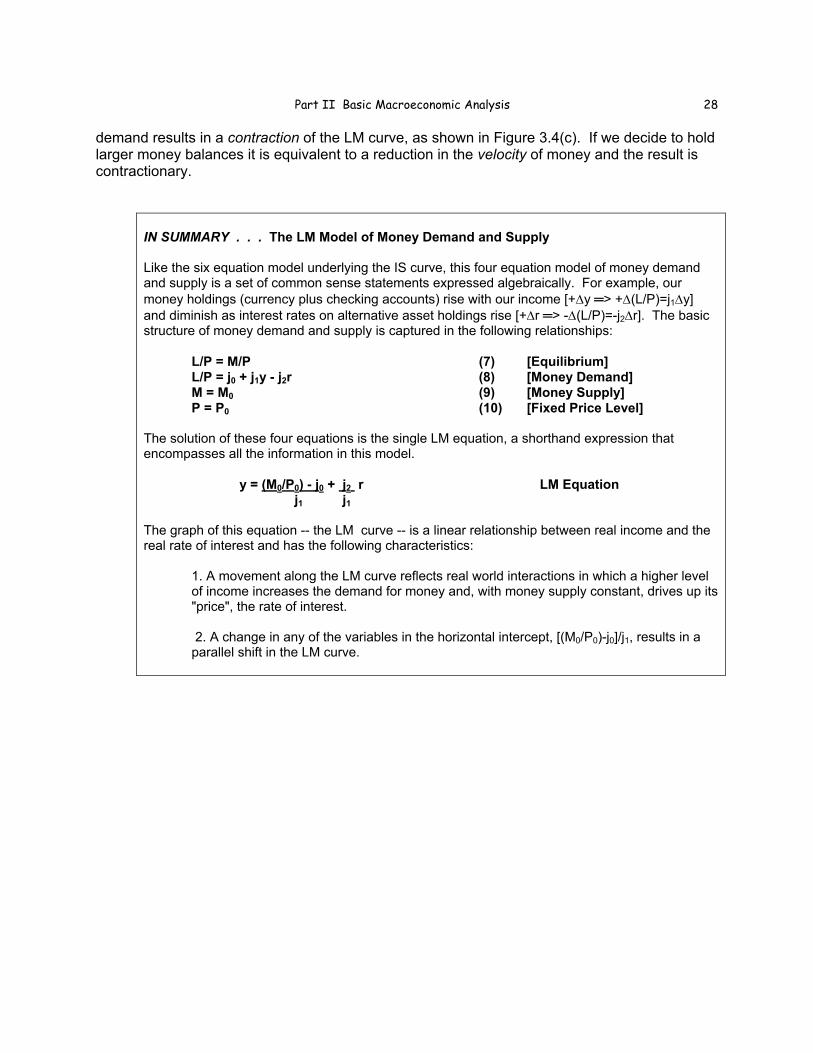
demand results in a contraction of the LM curve, as shown in Figure 3.4(c). If we decide to hold larger money balances it is equivalent to a reduction in the velocity of money and the result is contractionary.

IN SUMMARY . . . The LM Model of Money Demand and Supply Like the six equation model underlying the IS curve, this four equation model of money demand and supply is a set of common sense statements expressed algebraically. For example, our money holdings (currency plus checking accounts) rise with our income [+∆y ═> +∆(L/P)=j1∆y] and diminish as interest rates on alternative asset holdings rise [+∆r ═> -∆(L/P)=-j2∆r]. The basic structure of money demand and supply is captured in the following relationships:

L/P = M/P (7) [Equilibrium] L/P = j0 + j1y - j2r (8) [Money Demand] M = M0 (9) [Money Supply] P = P0 (10) [Fixed Price Level]

The solution of these four equations is the single LM equation, a shorthand expression that encompasses all the information in this model.

y = (M0/P0) - j0 + j2 r LM Equation j1 j1

The graph of this equation -- the LM curve -- is a linear relationship between real income and the real rate of interest and has the following characteristics:

1. A movement along the LM curve reflects real world interactions in which a higher level of income increases the demand for money and, with money supply constant, drives up its "price", the rate of interest. 2. A change in any of the variables in the horizontal intercept, [(M0/P0)-j0]/j1, results in a parallel shift in the LM curve.


3.10 The IS-LM Model of Aggregate Demand

The introduction to this group of five chapters (of which this is the first) portrayed this material as your "basic training" in macroeconomic analysis. This was a warning that the material would be difficult but essential. The main challenge for most students is not the level of analysis but the level of tedium. The derivation of the two-part IS-LM model of aggregate demand seems mechanical and lifeless, apparently far-removed from important issues of the real world. It may help you to know that the extensions and applications of subsequent chapters will breathe some life into this basic structure. This IS-LM model of aggregate demand will turn out to play a key role in your understanding of unemployment and the business cycle, stabilization policy, government deficits, monetary policy and interest rates, inflation, and international phenomena like trade deficits, exchange rates, and restrictions on trade.

This chapter, though long and involved, has explored just one question: "What factors determine the level of aggregate demand in the macroeconomy?". Chapter Two gave a much simpler but more primitive answer that assumed both market clearing and constant velocity of money. Both assumptions imply a very long run focus. Following the path blazed by Keynes, this chapter has implicitly dropped the constant velocity of money restriction in order to examine short run issues of aggregate demand. But in the process it has also opened up what looks like the proverbial can of worms—consumption, investment, and net export equations; parameters and policy instruments; expenditure and tax multipliers; and money demand equations. All these creatures are interrelated, intertwined, and very uninviting. It's definitely more complicated than the Classical long run approach. But it will turn out to be far more useful and, with a little practice, not nearly as forbidding as it looks just now.

The answer to "What determines the overall level of aggregate demand?" is contained in the ten equations (or sentences) of the combined IS-LM model. Remember that the six equation IS model was incomplete because it could determine the value of output/income (y) only if the real rate of interest (r) was already known. It gave a relationship between y and r (shown in the linear IS curve) but could not tell us where we were along that curve. It could tell us which events shift the IS curve (∆z0,∆g0,∆t0) and by how much (µ∆z0,µ∆g0,-c1µ∆t0) but, again, not where we'd end up along the new curve. More information was needed to complete the model of aggregate demand and this information was found in the four equation model of money demand and supply summarized by the LM equation and curve.

Putting IS (Equations 1-6) with LM (Equations 7-10) yields a complete model of aggregate demand, in which both y and r are determined, as are c, i, x, and other variables that depend on either income or the real rate of interest. Remember that underneath the deceptively simple veneer of the IS-LM graph, shown in Figure 3.5, is the elaborate 10 equation structure of aggregate demand. Though each of the 10 components is straightforward, together they are quite complex because of their interactions. Fortunately, with a little practice you will be able to use the compact IS-LM framework to get at some very important applications. In the following chapter, this model of aggregate demand is combined with a simple theory of aggregate supply to form the basic analytical framework used through the rest of the book.


3.11 Overview 1. This long and challenging chapter has led us from the simple, tranquil long run world of the Classical model to the more intricate and potentially stormy short run world of the Keynesian model. To John Maynard Keynes, the Classical dismissal of aggregate demand as a determinant of output and employment was absurd. He was especially critical of the contention that "fiscal policy is powerless" to influence output and employment. Keynes's response was to compose an alternative story (theory/model) in which demand played a significant, sometimes even dominant, role. 2. This chapter has developed an expanded model of aggregate demand based on Keynes's analysis. It requires some attention and patience. In your frustration, be careful not to slip back into the common view that "theory" is the opposite of "practical" and that models just make things more difficult than they really are. Economic models, however imperfect, are the most reliable maps we have. Without them, policy-makers are destined to sail in uncharted waters -- taking the economy and us along with them. Put another way, it is through models (and their embodied theories) that we attempt to decipher lessons from the past and transfer them to the present. It is not a choice between "theory" or "practice" or even between "theory" and "no theory". It's a matter of how carefully we use logic and past experience to understand the present and prepare for the future. 3. Aggregate demand (y), in Keynes's alternative to the Classical quantity theory of money, is divided into four categories -- consumption, investment, net exports, and government spending. More concisely, y=c+i+x+g, from which we build a model of total demand from smaller models of each component, namely c=c0+c1(y-t) and t=t0+t1y, i=i0-i1r, x=x0-x1y-x2r, and g=g0. Since total demand in equilibrium will be the same as total supply, we denote them both by the symbol y. This allows us to talk interchangeably of "income" or "output" since every dollar spent is a dollar received by someone. 4. The consumption-income relationship lies at the center of the process by which aggregate demand changes over time. A change in any of the four components of demand will initially change income by the same amount (since y=c+i+x+g). This stimulus will then be transmitted to consumption (since c=c0+c1(y-t)) which, in turn, alters income (again, y=c+i+x+g), which changes consumption again, then income, and on and on. This interaction between consumption and income means that any initial change in income is magnified through a multiplier process. Where all this interaction ends up is relatively easy to discover with some algebra and almost impossible without it. But easy or not, the important thing is to understand why this expenditure multiplier exists and what it implies for our ability to influence total demand in the economy. Review Section 3.4 until you have a comfortable understanding of why "the multiplier works in both directions," why "any ∆y sets off the multiplier process", and why "tax changes also have a multiple, though smaller, impact on total demand." 5. Once the basic logic of the multiplier is appreciated, it's not difficult to go beyond the consumption-income interaction (+∆y <═> +∆c) to see that because income taxes and imports rise with income, the size of the multiplier is reduced. In a nutshell, an initial rise in income starts the multiplier process through its impact on our consumption spending. But if part of that initial +∆y goes to the tax-collector (+∆t) and another part goes to purchase goods from other


countries (-∆x), less of it is left for +∆c in the United States. This, in turn, means a smaller subsequent increase in income hence smaller rise in consumption and so on, resulting in a smaller total effect on aggregate demand. Although these additional leakages reduce the size of the multiplier somewhat, it remains something to be reckoned with if we are to understand and attempt to control aggregate demand. 6. Another piece that must be added to our theory of aggregate demand is the fact that a change in the real rate of interest affects both net investment and net export spending. Specifically, there is an inverse relationship between the interest rate and these components of spending (+∆r causes -∆i and -∆x). Remember that since y=c+i+x+g, any change in i or x on the right hand side alters income and is then magnified by the multiplier process (e.g., -∆i & -∆x ═> -∆y <═> -∆c). 7. All these ingredients are incorporated in the expanded six equation model:

y = c + i + x + g (1) c = c0 + c1(y-t) (2) t = t0 + t1y (3) i = i0 - i2r (4) x = x0 - x1y - x2r (5) g = g0 (6)

The solution of this model, called the IS equation, is

y = µ(z0+g0-c1t0) - m(i2+x2)r , [IS Equation] where µ = 1/(1-c1+c1t1+x1) and z0 = c0+i0+x0.

8. Three important characteristics of the IS equation should be noted:

a. The algebra that gets us from six equations to a single solution (one equation) may look messy, but it's far easier and more practical than "common sense", "brute force", or other alternatives.

b The significance of this IS equation is that it is a true "bottom line". It takes into account the multiplier process (the interaction of equations 1 and 2, with leakages through equations 3 and 5) and the inverse relationship of aggregate demand and the real interest rate (Equations 4 and 5). It tells us that, all things considered:

i. a change in autonomous private spending (∆z0) or public spending (∆g0) affects income/output (y) through the expenditure multiplier (m) according to ∆y=µ∆z0 or ∆y=µ∆g0.

ii. A change in taxes (non-income for simplicity, ∆t0) affects income/output through the tax multiplier (-c1µ) as described by ∆y=-c1µ∆t0.


iii. A change in the real rate of interest (∆r) affects income/output (y) through its impact on investment (∆i) and net exports (∆x) as summarized by the sizes of the i2 and x2 parameters. This is then magnified by the expenditure multiplier (µ) and the final impact of a change in r on y is captured by ∆y=-(i2+x2)µ∆r.

c. Once you get the general picture of what's going on in terms of the algebra (a and b above), you can move them to the background and concentrate on the geometrical representation of the solution, the IS curve. It's easy to remember and easy to use.

i. The multiplier processes in b(i) and b(ii) above show up as parallel shifts of the IS curve by the amount of the ∆z0, ∆g0, or ∆t0 times the appropriate multiplier.

ii. The role of the real interest rate is captured in the downward slope of the IS curve, with an increase in r causing y to fall because of both the i2 and x2 terms and the spending multiplier, as given in part b(iii)

9. Much of the information needed to understand aggregate demand is incorporated into the IS equation and curve.

y = µ(z0+g0-c1t0) - µ(i2+x2)r , [IS Equation] where µ = 1/(1-c1+c1t1+x1) & z0 = c0+i0+x0.

Everything we need to know is either a policy instrument (values of which can be observed, forecast, or simulated) or is a parameter that can be estimated statistically except for one variable -- the real interest rate. The real interest rate (r) is not a constant that we can take as given. It's a variable that can and does change in response to many of the same things that alter aggregate demand itself. So without more information we're left in a situation in which if we knew r then we could find y and vice versa. But we don't, so we can't (and vice versa). 10. The needed information comes from the supply of money by the Federal Reserve and the demand for money by everyone who uses it. This is captured in the relatively simple "money market" model of equations 7-10 and summarized in the single equation solution, called the LM equation. L/P = M/P (7) L/P = j0 + j1y - j2r (8) M = M0 (9) P = P0 (10) y = [(M0/P0) - j0] + j2 r . LM Equation

j1 j1


11. Three characteristics of the LM equation should be noted:

a. The algebra that gets us from four equations to a single solution (one equation) is a bit messy, but easier and more useful than other alternatives.

b. The importance of this LM equation is that, like the IS, it is a "bottom line", taking into account the various factors influencing both money demand (namely, y and r) and money supply (the monetary authority).

c. Once you get the general picture of what's going on in terms of the algebra (parts a and b above), you can push it into the background and concentrate on the geometrical representation of the solution, the LM curve. It is easy to remember and use.

i. A movement along the LM curve reflects the fact that as income rises (+∆y), the demand for money also rises. (Remember that we can equate "aggregate demand" & "income" because every dollar spent is a dollar received.) And with a constant money supply this +∆y ═> +∆(L/P) puts upward pressure on the "price" of money. The result is that an increase in y leads to a rise in r.

ii. A change in any of the variables in the intercept term results in a parallel shift in the LM curve. For example, a +∆M0, -∆P0, or a -∆j0 shifts LM to the right, leaving the slope unchanged.

12. All this work has gone to answer a single but crucial question: "What determines the level of aggregate demand in the economy?". All the elements of the 10 equation model, summarized in the two solution equations/curves (IS and LM, Fig. 3.5) are necessary to give a reliable answer that, unlike the classical model, is applicable to the short as well as the long run. Chapter Four will pull this model of demand together, add a simple model of aggregate supply, and begin the applications that are the only justification for going to all this trouble. 3.12 REVIEW QUESTIONS 1. Define the following basic concepts or terms: Aggregate Demand Net Exports Price Index Income = Output Consumption Function Marginal Propensity to Consume Autonomous Consumption The Multiplier Process

The IS Equation The Expenditure Multiplier The Tax Multiplier Tax Function Net Export Function Autonomous Net Exports Net Investment Function Real Rate of Interest Autonomous Net Investment

Policy Instrument Parameter Money Demand Function Autonomous Money Demand Nominal Money Supply LM Equation The IS-LM Model of AD

2. In the simplest model of aggregate demand, we find that income changes by a multiple of any


change in government spending or autonomous consumption or investment spending. What basic interaction is built into that model that leads to this result? Explain how it works. 3. In the simplest model of demand there was neither an income tax nor an impact of changing income on net export spending. Once we add these two factors, the size of the multiplier declines. Show this algebraically and explain in common sense terms. 4. Suppose the government decides to reduce its deficit by $100 billion by cutting government spending. What will happen to the IS curve? Would your answer change if they raised taxes by $100 billion instead of cutting spending? Explain. 5. "If the government starts off with a balanced Federal budget and then increases spending by $20 billion, this will create a $20 billion deficit and shift the IS curve to the right. If the next year the government keeps its spending at this higher level and runs another $20 billion deficit, the IS curve will again shift to the right by the same amount." Evaluate. 6. Show that a change in autonomous money demand (∆j0) and a change in the money supply (∆M0) both shift the LM curve, but in opposite directions. 7. Show that a change in money supply (M) and the price level (P) both shift the LM curve, but in opposite directions. Use the LM equation to explain. 8. Suppose that two nearly identical countries both use fiscal and monetary policy to keep output at the same full employment level, but that Country A has higher taxes and a larger money supply than Country B. Government spending is the same.

a. On a single graph, show how the IS and LM curves of these two countries differ.

b. Compare the levels of each of the following variables for the two countries, i.e., higher, lower, or the same: consumption, investment, net exports, and the federal deficit.

9. Suppose there is a sudden increase in autonomous investment spending (+∆i0 in our model).

a. What impact will this have on equilibrium y and r? Explain.

b. Suppose the Federal Reserve reacts to this event (+∆i0) by changing M so as to move r back to its original level. What will happen to equilibrium y? Explain.

c. Instead, suppose the Fiscal authorities react by changing g so as to move r back to its original level. What will happen to equilibrium y? Explain.

10. "The IS-LM model cannot be more than a partial explanation of economic activity, because it implies that monetary or fiscal policy (or both together) could be used to push y to any level we desired." Do you agree or disagree? Explain.


11. a. Suppose the economy is initially in short run equilibrium below full employment and policy-makers decide it's time to take strong actions to restore full employment (y*). They decide to do this with fiscal policy, but want to do it in a way that causes the smallest increase in the already large government deficit. They ask you to devise a plan to accomplish this. What would you recommend? Explain. b. Your proposal is immediately attacked by an influential Senator as short-sighted and irresponsible. She says that it might work, but only at the cost of a larger deficit and a smaller rate of capital formation hence slower long run economic growth. (Note: "economic growth" refers to changes in y* while "economic recovery" is the return of y to a given y*.) She advocates the use of monetary policy instead, arguing that this will not only restore full employment but actually reduce the budget deficit and increase economic growth. Evaluate her proposal and (if you can) defend your own. c. The chairman of the Descendants of Adam (Smith) Society attacks both you and the Senator for your knee-jerk invocation of government policy. Your "visible fist", as he calls it, is neither needed nor welcome. He says you have forgotten that basic market mechanics ensure that yAD>y* ═> +∆P, yAD<y* ═> -∆P, and yAD=y* ═> ∆P=0. Adding this ingredient to the IS-LM model of aggregate demand, he concludes that we will not only return to full employment automatically but also in a way that stimulates growth and reduces the deficit—and all without the use of any centralized policy manipulation. Evaluate his proposal. 12. In equilibrium in the Keynesian model, the real money supply (M0/P) equals real money demand (L/P=j0+j1y-j2r). Equilibrium in the "money market" is then M0/P=j0+j1y-j2r. Show that in the Classical model (with constant velocity of money) the analogous money market equilibrium is M0/P=(1/V)y and graph this relationship in terms of (y,r)-space (i.e., with the same axes as for the IS-LM graph). In other words, what does the graph of the Classical LM curve look like? Explain.

Documents

THE KEYNESIAN MODEL OF AGGREGATE DEMANDmcelroy/302/E_Chpt3.pdf · The concept of aggregate demand has four important characteristics: 1. ... Chapter 3 The Keynesian Model of Aggregate