The peculiar economics ofbalanced multiregional growth

under constrained resource usageS. J. Nettleton1

1 University of Technology Sydney, Australia (corresponding author stuart.nettleton@uts.edu.au)

AbstractMainstream computable general equilibrium analysis developed out of Lief Johansen's regional economic analysis based on the simultaneous settlement of commodity markets in quantity and price. The work of John von Neumann, Paul Samuelson, Wassily Leontief, Anne Carter, MichaelFarrell and Thijs ten Raa has combined in an alternative bottom-up Integrated Assessment Model, which embodies Johansen attributes while exploiting the unique property of models having regions that trade and adjust to evolving natural advantages and environmental constraints through regional industry specialization. Such specialization has recently become a major focus in many nations seeking competitive niche business models in intermediate products and capital goods, which today comprise 70 per cent of the global supply chain. This research demonstrates a non-monetary or policy application of the Doctrine of Balanced Growthoperates to equalize consumption growth at the policy nexus of international free-trade agreements and specialization of regional industry segments. Our knowledge of domestic industry policy and international trade policy is advanced by this demonstration that model results conform with a non-monetary Doctrine of Balanced Growth. This study is based on 2007 year data from the Global Trade Analysis Project.

Keywordsdoctrine of balanced growth, integrated assessment model, computable general equilibrium, intertemporal optimization, dynamic optimization, optimal control, macroeconomics, growth, environmental constraint, industry specialization

1. IntroductionThe Doctrine of Balanced Growth has been widely discussed in the areas of economic growth, public finance and international trade. Lief Johansen's investigations led him to develop the first comprehensive Computable General Equilibrium (CGE) model to investigate monetary applications of the Doctrine. The research in this paper investigates the non-monetary or policy application of the Doctrine of Balanced Growth. The Motivation introduces the research question, background to the monetary Doctrine of Balanced Growth and policy utility functions based on Normative Ethical Theories. Data sources for the Integrated Assessment Models (IAM) are discussed. Important Identification Strategy elements include the structure of the IAM and in particular commodity prices, inherent Cobb-Douglas Production Function, and the specific IAM used, which is the Spatial Climate Economic Policy Tool for Regional Equilibria. Computational strategy is an important part of Identification so an illustrative toy problem is usedto evaluate Direct and Indirect techniques to evaluate the optimal controls that often occur in economic and engineering applications. Results of the IAM Computational Strategy are presented. Results of the investigation into the research question using the IAM and the Computational Strategy are presented and discussed.

2/32

2. Motivation

2.1 Research QuestionThis empirical investigation was motivated by Lief Johansen’s investigation into the Doctrine of Balanced Growth as a convenient point of policy intervention to stimulate economic growth (Johansen, 1974); the modern trend towards free trade agreements; and the pressing need for nations to establish competitive niches in global supply chains for intermediate and capital goods and services.

This research uses Integrated Assessment Modeling (IAM) to evaluate the Doctrine of BalancedGrowth at the nexus between domestic industry policy and international trade policy.

The IAM is applied to address the research question of whether balanced regional consumption growth emerges where regions with diverse production functions freely trade in the presence of deficit and geophysical constraints, Total Factor Productivity growth and harmonious policies for international trade relations, analogous to competition with cautious trust in infinite games (Ricardo, 1817).

Three regions are modeled: the North America Free Trade Association (NAFTA), the original 25 country European Union (EU25) and the Rest of the World (ROW). The Rest of World sector, which is comparatively underdeveloped compared to the NAFTA and EU25 regions, enjoys the same growth path as the developed regions.

The key finding is that free trade with balanced trust strategies in international trade brings similar or balanced consumption growth to each of the trading regions. In addition, regional industries specialize through trade opportunities, which is necessarily constrained by limits to regional trade deficits.

With the research question is answered in the affirmative, the non-monetary Doctrine of Balanced Growth can be promoted as a policy to maximize the balanced economic growth of the participant trading regions in the presence of free trade.

The modeling in this research helps clarify three unusual aspects of the Doctrine of Balanced Growth. The first aspect is the contrast between the underlying concept of the Doctrine of Balanced Growth and its observed application. The Doctrine of Balanced Growth was first proposed for isolated underdeveloped countries with low purchasing power (Nurkse, 1966). However the large public debt implications have deterred policy makers in these countries from attempting to implement it.

Conversely, while the economic non-Keynesian basis of the Doctrine of Balanced Growth remains contentious, developed countries have routinely applied industry assistance interventions such as investment allowances during cyclical downturns in to stimulate idle production capacity, employment and consumer demand (Misra and Puri, 2012).

3/32

The second aspect of the Doctrine of Balanced Growth is that it refers to broad policy intervention across industry sectors to stimulate growth in production. In regard to consumption, the implicit direction of causality is analogous to Say's law, that production creates its own consumption (Say, 1803). Increased output across the network of intermediate production is seen as catalyzing increased labor demand and ultimately consumption. However, an isolated economy producers lack the ability to utilize new found productivity to capitalize on advantages for export markets. For the same level of output, targeted investment in Total Factor Productivitymay reduce intermediate commodities and factors such as assets and labor. In addition, capital may substitute for labor in production functions. Policy makers have long recognized that a naive implementation of the Doctrine of Balanced Growth in an isolated underdeveloped economy may be counter productive (Johansen, 1974).

The third aspect of the Doctrine of Balanced Growth is that the productive sector remains a convenient point for stimulatory policy intervention. It is also harmonious with a capitalist world view and early general equilibrium models were generally underpinned by the perspective of producers' profit maximization (Johansen, 1974). In contrast, modern approaches to general equilibrium maximize consumption utility, which reflects the social mandate. In practice, it is often as convenient for policy makers to directly stimulate consumption (e.g. “cash for clunkers”)as it is to stimulate production.

This research extends a single economy approach (Raa, 2005) into a multiregional trading model that is intertemporal and constrained, where producers are able to develop specializations through productivity and restructuring that capitalize on natural advantages. The main issues to be covered and discussed are the relationship between the theoretical framework of an IAM based on multiregional computable general equilibrium and models in the tradition of Johansen; multi-objective utility functions suitable for cautious trust strategy games in international trade relations; and the optimization of intertemporal optimal control functions across the underlying dynamic systems in the presence of trade deficit and priced-environmental geophysical feedback constraints, and Total Factor Productivity growth.

This modeling research complements the research topic of future national business models in intermediate products and capital goods, which comprise approximately 70 per cent of the global supply chain. This has recently become a major focus in many nations seeking sustainable wealth creation and employment in structurally weak economies characterized by scarce investment opportunities, perhaps notwithstanding an excess of savings (Bernanke, 2005).

Addressing the research question is important for understanding the structure of modeling constrained multiregional policies; setting new directions in the evolution of IAMs in climate change modeling; and for establishing new functional optimal controls computation techniques for policy modeling.

The main result of this research is that a virtuous path of balanced consumption growth is present in both advanced and developing economies, which are diverse trading economies with unique production and adaptation properties. This is a practical demonstration of the Doctrine ofBalanced Growth in international trade. It highlights that international policies that promote trade

4/32

can deliver high growth although regions will need to be proactive in pursing industry specialization and vigilant in the sharing the mutual benefits of industry specialization in various regions.

2.2 The Doctrine of Balanced GrowthJohansen was focused on the “basic complementarity” between different industry sectors in a single well-developed market economy, observing that one of the main areas for simultaneous consideration of all production sectors was in policies for balanced economic growth (Johansen,1974, pp. 5–8).

The Doctrine of Balanced Growth, which was originally proposed for underdeveloped countries, hypothesizes that significant government investment in production productivity, both widely and simultaneously in many industries and sectors, to expand consumer purchasing power and overall market demand and attract private investment can convert a cycle of poverty into a virtuous circle of economic growth (Nurkse, 1966, p. 163; Srinivasan, 1988, p. 882).

There has always been abundant empirical support for the Doctrine of Balanced Growth in terms of simultaneous positive trends in production, consumption and investment (Klein and Kosobud, 1961). Traditional tests for the Doctrine of Balanced Growth have assumed that it necessarily requires constancy or stationarity in the great ratios of consumption and investment to production (Kaldor, 1961), although not necessarily in the ratio of savings to investment (Kuznets, 1942). Initially stationarity in the great ratios was shown in the UK (Mills, 2001) but notfor other industrialized countries (USA (Klein and Kosobud, 1961), Canada (Serletis, 1994), Australia (Kunst and Neusser, 1990), China (Li and Daly, 2009) and OECD and G7 countries (Harvey et al., 2003; Serletis and Krichel, 1995)). However, stationarity was determined for the USA (Attfield and Temple, 2010) after taking into account mean shifts in the economy due to changes in underlying structure.

These studies regarded government intervention as being monetary stimulation. This research provides a major point of difference with earlier investigations in considering the non-monetary application of the Doctrine of Balanced Growth. This is policy intervention through multiregional free trade agreements at an international level with the Ricardian (Ricardo, 1817) aim of buildingthe prosperity of all regions. It also overcomes the apparent anomaly in analyzing the Doctrine of Balanced Growth using a free-market neoclassical growth model where governments have little opportunity to play a significant role in the growth process.

2.3 Policy Utility FunctionsJohansen's model and the Doctrine of Balanced Growth each sought to maximize producers' profit and in doing so increase consumers' welfare. However, policy makers subsequently became more interested in directly maximizing consumers' welfare while interpreting consumer behavior and the path of consumption (Barro and Sala-i-Martin, 2003; Cass, 1965; Koopmans, 1965; Ramsey, 1928). Johansen compared his multisector model with a hybrid intertemporal model (Kendrick and Taylor, 1969) that used optimization to maximize consumers' utility (Johansen, 1974, pp. 180–1). He concluded that the optimization framework replaced many of

5/32

the consumer, producer and capital stock behavioral equations introduced in his own model andthat consumption growth would follow the demand functions corresponding to the utility function.

A stationary maximum in analytical analysis and “optimize then discretize” strategies requires the consumer utility function to be twice differentiable and concave, for example the traditional saturating Constant Intertemporal Elasticity of Substitution (CES) utility function, which is Arrow-Pratt's Constant Relative Risk Aversion (CRAA) criterion (Arrow, 1965; Pratt, 1964). The well-known Keynes-Ramsay Rule for maximizing consumption utility subject to capital is the second or Euler equation of the Ramsay-Cass-Koopmans model as shown in Figure 1 (Cass, 1965; Koopmans, 1965; Ramsey, 1928).

Figure 1: Ramsay-Cass-Koopmans Model Euler Equation

It may be noted that increasing the Coefficient of Relative Risk Aversion θ reduces the rate of growth of consumption, thereby placing greater value on the consumption in later periods. Present value discounting offsets this intertemporal effect. Increasing the required utility rate of return ρ decreases the rate of growth of consumption and thereby reduces the value of future consumption.

However TFP growth holds the promise of future generations being better off since consumptiongrowth is underpinned by progressively greater production with the same capital stock and investment (or even capital stock having a declining characteristic). Some policy makers therefore dispute the basis for inter-generational trade-offs and prefer the simplicity of an instantaneous consumption utility function. In addition a pure consumption utility function has animportant advantage, which is that shadow prices are in standard monetary units rather than utility units that are more difficult to interpret.

However, consumption c alone does not meet the requirement of being twice differentiable and concave. In fact it might be expected that consumption may never have a saturating characteristic if both annual growth in Total Factor Productivity (TFP) and regional specializationof industries continuously enhance the profitability of industries. So the performance of a utility function such as consumption alone is instead limited by the presence other equality and inequality constraints such as those provided in an IAM.

Using a consumption utility function also requires a different computational strategy than the analytical or “optimize then discretize” approaches. The reverse non-analytical “discretize then optimize” strategies do not impose any special requirements on the concavity of the utility

6/32

cc

=r−ρθ

Where :c consumptionr interest rateon savingsρ the discount rate of consumptionθ coefficient of relative risk aversion1/θ inverse of elasticity of intertemporat substitution

function if the utility function and resource and other constraints determine the position of the global maximum at any time and ultimately the path of consumption growth. In this regard, both the CES and instantaneous consumption utility functions are equally satisfactory.

"Discretize then optimize” strategies are ideally suited to real problems where the theoretical requirement for utility functions to be twice differentiable is inconvenient. For example, in expanding the scope of a constrained optimal controls problem from a single region to a multiregional scenario, the utility of each region needs to be in some way maximized and contemporaneously settled with the performance of the other regions. There are various multiple agent goal programming optimization techniques for achieving this contemporaneous settlement (Charnes et al., 1955; Charnes and Cooper, 1961).

Arising from a social context, the selection of an objective inherently embody ethical judgments. Seen from this perspective, the choice of a utility function is equivalent to selecting a social policy for the economic development. The three oldest, most widely used but often least theoretically justified forms of goal programming are the Archimedean (also called a Merit function or dominant equilibrium), non- Archimedean and Maximin functions. (Romero, 2004)

The different social policy perspectives can be interpreted in terms of the Normative Theory in Ethics. There are two primary groups of theories: the Teleological or consequences-based theories and the Deontological or duties-based theories (Dellaportas et al., 2005).

The Teleological group of theories comprises both individual profit seeking, known as Ethical Egoism, and Utilitarianism, which is seeking the best outcome for the greatest number of peopleconsidered as a whole, deriving from the work of Jeremy Bentham (1748-1832) and John StuartMill (1806-73). The Teleological approach is readily modeled with an Archimedean (Merit function) objective. Examples are the weighted sum of profit or of the utilities of the competing agents. If the weights are all unity then the Archimedean objective is a merely simple sum. Depending upon the structure of equality and inequality constraints, the Archimedean approach may lead either to a single dominant equilibrium or develop into an infinite set of solutions across a Pareto-efficient trade-off frontier. A dominant equilibrium is also a Nash Equilibrium, where each region has played to its comparative strengths and with full knowledge of the strengths and weaknesses of competitive trading regions is disinclined to change its position.

Consistent with the Teleological foundations, an Archimedean optimization often results in a winner-takes-all outcome. For example, in a regional growth context, each region may pursue its own best growth outcome irrespective of the strategies of other regions. Furthermore, those regions that are better position to grow may do so at the expense of strategically weaker regions.

Another issue with Teleological utility functions is that the outcome cannot be predicted in a rational behavior model. For example, in regard to Ethical Egoism, the enlightened self-interest perspective might be exceptionally vulnerable to selfishness behavior, which in turn may damage confidence in the social mandate that permits the operation of a free trade market (Kahneman and Tversky, 1979; Tversky and Kahneman, 1992). Pure Utilitarianism can be similarly flawed since decisions based solely on the criterion of greatest good for the greatest

7/32

number of people have, throughout history, proven to be highly risky, for example, leading to authoritarian regimes and even morally corrosive in being used to justify great wrongs such as slavery.

The Deontological group of theories introduces principles of social justice. It comprises the theories of rights (Immanuel Kant, 1724-1804) and distributive justice (Aristotle, 384-322BCE). Progressing long term social stability in a modern society whilst at the same time promoting change and growth usually requires tuning the ever-emerging balance between the theories.

The Deontological approach is based on the premise that the market and its participants have duties (or obligations) to the social system, which has granted producers the mandate to operate. The first component of the Deontological approach is Rights Theory, for example the right to freely trade. While at first glance a Rights Theory appears to be solid principle, there are two major issues. These are that some rights have preference to other rights and not everybodyvalues particular rights in the same way. A modified Archimedean objective, called non- Archimedean has some analogy with Rights Theory. It uses lexicographic or preemptive functions to preferentially satisfice constraints and weight or rank the objective function.

The second component of the Deontological approach is Justice Theory. This theory holds that benefits and costs should be fairly distributed across society (or market participants) such that to each goes a fair share based on the three criteria of merit, effort and need. For example, Rawls' Theory of Justice (Rawls, 1972) is based on the premise that social stability depends upon people having been fairly treated and protected from morally wrong acts such as injustice, corruption and nepotism. Rawls draws parallels with the von Neumann's Maximin principle (Von Neumann, 1928) such that everyone may be better off by a particular policy as long as no-one is worse off. For example, that benefits and costs are distributed equally except where a varied distribution will better work to everyone's advantage.

Deontological Justice Theory may be modeled by Maximin goal programming (also known as Chebyshev or Fuzzy Programming) (Flavell, 1976). This form of utility function seeks a single best solution that minimizes the maximum of disadvantage amongst the agents compared to a benchmark. In other words, it maximizes the minimum deviation. In a regional trading context, all regions seek to maximize their growth while at the same time moderating their behavior for a game strategy characterized by an infinitely long-term outlook; highly repetitious behavior; the potential for irrational response behavior and tit-for-tat strategies; and an ability for regions to change structure and policies to remain competitive. In this environment, trade optimization often takes account of the need for all regions to share in growth and to limit the worst outcome in any region. Therefore the result of a Maximin strategy is not necessarily profit maximizing in each region but a conservative choice of long-term international relations policy in the presence of repeated interactions recognizing that regional behavior may change and may become irrational if there is a disproportionate sharing of the benefits of growth.

In real social optimization problems, a combination of Archimedean and Maximin provides a sound balance between objectives of maximum aggregated achievement and the most balanced solution (Romero, 2004). In this research a 50/50 blended Archimedean/Maximin

8/32

utility function provides a stable outcome based on both the pursuit of comparative advantage along with game theory applicable to infinite horizon games in international bi-lateral relations.

To the author's knowledge, nobody has ever undertaken a multiregional IAM with 50/50 blendedArchimedean/Maximin objectives, while allowing sectors to grow through specialization as a function of free trade. This is a compelling innovation.

3. Data

3.1 Social Accounting Matrix

The regional Make and Use tables used in this research are sourced from the Global Trade Analysis Project (GTAP) Social Accounting Matrix (SAM) (McDonald and Thierfelder, 2004) version 8.1 for the 2007 year. The 134 representative countries are aggregated into three major trading regions: North America Free Trade Association of USA, Canada and Mexico (NAFTA); original 25 country European Union (EU25); and the Rest of World (ROW).

The 57 commodities across the regions are aggregated into three major commodity groups: Agriculture, Forestry and Fishing (agff); Manufacturing and Mining (mnfc); and Services (serv). In each region, Final and Government consumption are combined. Bilateral trading between regions is recorded along with transport and other margins. Greenhouse gas permit trading and adaptation/amelioration commodities expand the intermediate production Make and Use tables to five by five. Greenhouse gas estimates are obtained from the GTAP emissions database (Lee, 2008).

3.2 Labor Factor

Regional labor is assumed to follow population growth in the region. Regional population profiles are developed within the envelop of global population, which is estimated to grow in the nature of a sigmoid from 6.514 billion to eventually stabilize at 8.6 billion people (Nordhaus, 2008). The labor force in each region is assumed to contribute to this profile with a unique sigmoid where the initial parameters of the weighted growth rate and total population characteristics of the countries comprising the region. These initial parameters are: NAFTA (432m, 1.0%pa), EU25 (460m, 0.26%pa) and Rest of World (5,622m, 1.2%pa). The components of the population profile are shown in Figure 2 (below).

9/32

3.3 Capital Factor and Accumulation

The capital factor provided within a GTAP Social accounting Matrix is the dollar return on capitalstock by region and commodity. Conceptually this represents the total capital stock employed byfirms in each region in producing a particular commodity, multiplied by the average rate of returnon capital for the region commodity segment.

Capital accumulation is the central dynamic feature of all intertemporal CGE models. Capital stock is subject to the usual accounting process where it grows with investment and declines with depreciation and disinvestment. Where models permit industries to specialize through international trade, capital resources may redistribute across regional industries that industries are no longer restricted by the fixed proportions of their production technology. The capital factoris a return on capital stock so total capital factor endowment does not constrain the sum of the capital factor usage in the production of each commodity.

The capital constraint may instead be implemented by requiring that the per unit growth in capital stock for a region commodity segment equals the per unit growth in industry activity production. This is because capital stock will change proportionally with production if: a per unit change in production leads to the same per unit change in dollar return on capital stock; the capital stock returns in each region-commodity segment remain approximately constant with increases or decreases in the production multiplier; and Total Factor Productivity increases output from the adjusted Make less Use matrix, which in turn lessens the production (and labor) multiplier that would otherwise be required for the same output. This is similar to a DuPont Analysis assets to sales ratio reduced by Total Factor Productivity. It also satisfies the competitive requirement of constant or decreasing returns to scale in an economy, considered both at the local and global trade-linked levels. In each case an increase in production leads to less efficient firms with higher cost structures entering the commodity segment, consistent with a Cobb-Douglas production function and marginal costs that are greater than or equal to average costs (Houthakker, 1956; Raa, 2005, pp. 103–7).

On a practical level, obtaining the Capital Stock and Depreciation for each region-commodity segment can be challenging. GTAP provides the total Capital Stock Value at Beginning of

10/32

Figure 2: Regional Population Projections

Period for each region but this lacks detail at the commodity level. Furthermore, Capital Stock Depreciation is set at a uniform 4%pa.

A number of the larger national statistical agencies conduct special studies to estimate the capital stock and depreciation in each industry. From a representative sample of these studies weighted averages have been developed for the Industry Asset Mix and Depreciation Rate for each region / commodity segment as shown in Tables 1 and 2 (ABS, n.d.; NBS, n.d.; OECD, n.d.; US Department of Commerce, n.d.; Wu, 2009).

Asset Ratio NAFTA EU25 ROW

Agriculture, Forestry & Fishing 1% 3% 7%

Manufacturing & Mining 10% 12% 27%

Services 89% 85% 66%

Total 100% 100% 100%

Table 1: Estimated Regional Asset Mix

Annual Depreciation Rate NAFTA EU25 ROW

Agriculture, Forestry & Fishing 7.6% 7.6% 6.1%

Manufacturing & Mining 9.9% 8.6% 6.6%

Services 4.6% 4.6% 4.9%

Table 2: Estimated Regional Asset Annual Depreciation Rate

From these weighted averages, Capital Stock and Depreciation by region and industry may be estimated using GTAP’s assets by region (Purdue University Department of Agricultural Resources, 2013). A factor control for Land is not treated separately as all of the Land factor return is concentrated in Agriculture, Forestry & Fishing and the redistribution to Manufacturing & Mining and Services would not be meaningful.

4. Identification StrategyThis empirical investigation was motivated by Lief Johansen’s investigation into the Doctrine of Balanced Growth as a convenient point of policy intervention to stimulate economic growth, as part of developing his multisectoral computable general equilibrium model (Johansen, 1974); the current pressing need for nations to establish competitive niches in the global supply chains for intermediate and capital goods and services; and the modern trend towards free trade agreements.

The research question is an empirical hypothesis that a shared international trade policy leads to balanced growth in trading economies based on optimizing a combined 50/50 Archimedean (or Merit) and Maximin multi-objective utility function for economic growth derived from Normative Ethics Teleological and Deontological Theories.

11/32

This research question is investigated using an intertemporal, dynamic, continuous multiregionalCGE model in the presence of global constraints. This model identifies the global maximum utility by varying investment, trade and adaptation parameters, to distribute production across regional industry niches, according to natural advantage in production functions and labor. The model is native as it requires only one exogenous assumption, which is the profile of global population growth. All other parameters are derived from national accounts and statistical agency surveys.

A potential deficiency in the research model is that only three aggregated regions (NAFTA, EU25 and ROW) with five commodities (food, manufacturing, services, greenhouse gas permits and greenhouse gas abatement) are investigated. The number of regions and commodities are limited because of the magnitude of the optimization task in locating the optimal control functions for a utility function having many global sub-maxima across a continuous multiregionalCGE model, requiring the solution of differential equations.

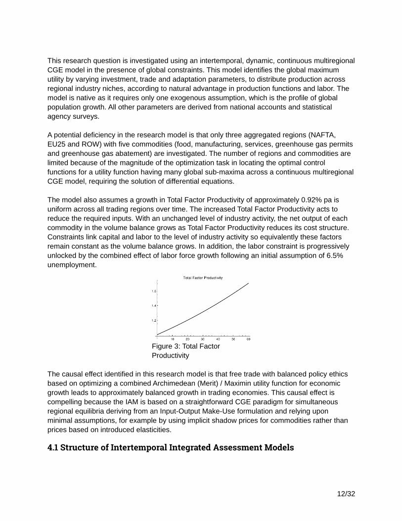
The model also assumes a growth in Total Factor Productivity of approximately 0.92% pa is uniform across all trading regions over time. The increased Total Factor Productivity acts to reduce the required inputs. With an unchanged level of industry activity, the net output of each commodity in the volume balance grows as Total Factor Productivity reduces its cost structure. Constraints link capital and labor to the level of industry activity so equivalently these factors remain constant as the volume balance grows. In addition, the labor constraint is progressively unlocked by the combined effect of labor force growth following an initial assumption of 6.5% unemployment.

The causal effect identified in this research model is that free trade with balanced policy ethics based on optimizing a combined Archimedean (Merit) / Maximin utility function for economic growth leads to approximately balanced growth in trading economies. This causal effect is compelling because the IAM is based on a straightforward CGE paradigm for simultaneous regional equilibria deriving from an Input-Output Make-Use formulation and relying upon minimal assumptions, for example by using implicit shadow prices for commodities rather than prices based on introduced elasticities.

4.1 Structure of Intertemporal Integrated Assessment Models

12/32

Figure 3: Total Factor Productivity

Since the 1960s, the novel and innovative concepts arising from Computable General Equilibrium (CGE) have seen CGE become established practice within policy formulation in almost every part of the world. While CGE models have many purposes, such as single country or multiregional models, single period or intertemporal projection models, and different solution approaches, this research focuses on multiregional models, which have been extensively reviewed (Donaghy, 2009; Giesecke and Madden, 2013; Kraybill, 1993; Partridge and Rickman, 1998).

In this research an Integrated Assessment Model (IAM) is used to demonstrate the Doctrine of Balanced Growth amongst international regions that trade. IAMs often build on CGE models that have been extended with satellite physical resource and environmental data. IAMs provide a sound economic framework for policy discussion and highlight many issues that are not immediately apparent to researchers. For example, IAMs can be used to help answer industrial ecology questions such as “what happens if the atmospheric temperature increases? “

Perhaps the most common diagnostic questions present in most social, economic, environmental and infrastructure applications of IAMs are: economic development within economies connected through bilateral trade, the evolution of regional industry comparative advantages in mutual response to changes happening in the other economies and how these things are moderated by environmental constraints. For example, strategies for efficient value-adding sectors can be developed from the time profile of industry activity under constrained resources and the networked effects on household consumption; the positive effect of technology (or pollution control) on consumption and spillover improvements to trading regions; the negative effects of subsidized technologies on the activation of unexpected sectors in the economy and adverse impacts on consumption. This information is particularly important for small open economies that have a strong dependence on raw material exports, such as Australia and Canada.

Although CGE principles stem from the work of Léon Walras (Walras, 1877), modern IAM policy applications commenced with the coming together of a systematic approach to economic data (Leontief, 1966, 1955), a demonstration that general equilibrium could really exist in an economy (Arrow and Debreu, 1954; Debreu, 1959) and the computable modeling approaches ofJohansen (Johansen, 1974) and development of optimal controls (Dorfman et al., 1958; Von Neumann, 1938).

Most IAMs that are based on CGE principles, such as hybrid Input-Output life cycle models, build on Leontief's Input-Output Analysis, which is an elementary form of CGE that resolves industrial flows in networked production (Leontief, 1941, 1936). Its main strength is a robust microeconomic foundation for partial equilibria in production and consumption having a macroeconomic flavor by virtue of using whole economy empirical data. The straightforward nature of Leontief's Input-Output Analysis makes it popular for investigating industry competitiveness, the multiplier effects from investment and the effect of environmental restrictions on prices and structural path. The major weaknesses in Input Output Analysis are that it treats investment similarly to consumption; there is no substitution between industries via the route of international trade; and consumer behavior is not addressed because final demand is typically exogenous.

13/32

Differences in computational methods for behaviorally settling resource prices are a major differentiating feature within the more comprehensive CGE frameworks. Johansen's well-known top-down approach simultaneously settles the economic actor behavior of producers, consumers, government and capital providers. Johansen develops a set of equations by analytically maximizing producers' profit and augmenting these equations with dynamic growth in productive assets, material balances (in lieu of the budget equation of consumers) and supplyand demand settlement through a system of prices with exogenous elasticities (Johansen, 1974, pp. 27–9). Mainstream CGE frameworks traditionally follow Johansen to settle in both volume and price at competitive valuation by endogenizing investment, consumption, changes in the vintage structure of productive capital, changes in industry activity and employment, tradeflows and foreign debt. A Johansen-type CGE model is firstly balanced and then used to understand the effect of “shocks,” which are “what if questions” that perturb the steady-state, such as what if industry productivity increases? What if trade tariffs decrease?

4.1.1 Shadow pricesVon Neumann first recognized that Input-Output material balances could be represented as resource inequalities within an optimization study. The approach was adopted in studies of technology in national production functions and structural change (Carter, 1970; Raa, 2008). It was then further developed into a comprehensive theoretical basis for CGE (Raa, 2005).

The key advantage in using an optimization method across resource constraints is that the marginal productivity of additional units of each resource are automatically calculated in the dualsolution to the optimization's primal problem (Champernowne, 1945; Hotelling, 1932; Houthakker, 1960; Samuelson, 1953; Von Neumann, 1938). These marginal productivities are closely related to commodity market prices, which are called the shadow prices and are similar to Lagrange multipliers, denoted by the Greek letter lambda (λ) in honor of Joseph Louis Lagrange (1736-1813). The Theorem of Complementary Slackness provides that resource constraints are either binding and prices emerge, or non-binding and prices are zero. The emergence of prices at binding constraints is known as von Neumann's knife-edge specialization. Von Neumann's knife-edge assumptions also have great importance for national employment in a global equilibrium in the presence of free trade. When a country subsidizes its exports then unemployment rises elsewhere (Samuelson, 1964, p. 146).

4.1.2 Cobb-Douglas production functionLabor capital substitutability in networked production functions is often considered a second major differentiating factor in models but the issue usually reduces to whether labor substitution is treated explicitly or implicitly. For example, Johansen-like models typically treat labor explicitlyusing CES functions and more specifically the Cobb-Douglas production function, which has become the main neoclassical tool of macroeconomics. Similarly, CES functions have often been used to model the substitution between labor and capital in Input-Output sectoral production functions.

However, there is an important substitution between capital and labor that occurs across sectorsin optimal controls models that operate directly on Supply and Use tables (Raa, 2005, pp. 93–103). These inherent substitutions across sectors are a very powerful innovations in a

14/32

multiregional context because regional sector growth may occur through specialization. In other words, the sector may choose a production technique as a function of free trade rather than being restricted by the fixed proportions of their production technology and fixed import coefficients (Raa and Baumol, 2011). An important observation is that the resulting macroeconomic production function is Cobb-Douglas (Houthakker, 1956; Raa, 2005, p. 105).

4.1.3 The Spatial Climate Economic Policy Tool for Regional Equilibria

The particular type of intertemporal IAM used in this research, the Spatial Climate Economic Policy Tool for Regional Equilibria (Sceptre), is a multiregional CGE focused on reducing inefficiencies and rewarding efficient industries [(Nettleton, 2010a, 2010b; Wolfram, Inc., 2011). Implicit in the multiregional context is the importance of policy analysts diagnosing inefficiencies arising from the lack of orientation of the economy in its trading context, the misallocation of sector activity and the inefficient utilization of factor endowments within sectors. From this, strategies for efficient value-adding sectors that can benefit from increased specialization in the economy to correct these inefficiencies can be identified. With this “open” approach to the production mix, production is reallocated according to the comparative advantage of regions (and imports), factors are reallocated across sectors within a region, and substitution takes place between capital and labor between sectors.

Optimal controls for industry activity and trade that maximize the time discounted 50/50 Archimedean (or Merit) and Maximin expansion in consumption as shown in Figure 4.

Figure 4: Objective Utility Function (equally weighted Archimedean and Maximin)

Prima facie regional industry investment would be a more intuitive control than industry activity. However, in Sceptre industry expansion replaces regional investment because extensive research into the use of regional investment determined it to be unstable as a functional control.

The necessary reallocation of industrial activity and changes in consumer behavior in Intertemporal IAMs is achieved through Data Envelopment Analysis (DEA), which evolved from Samuelson's linear programming and Farrell-benchmarking (Farrell, 1957; Raa, 2005). Growth of the consumption basket is maximized by eliminating inefficiency in production and net importsso economies will operate to their maximum efficiency given their natural endowments and structural production functions. A key advantage of this approach is that it bypasses imposed hypothetical behavioral assumptions in consumption and production, including the inherent but sometimes rather tenuous price elasticity assumptions. Using these techniques, optimal controlsmodels that operate directly on Supply and Use tables compute an equilibrium directly from the data of national statistical agencies with few assumptions.

15/32

e−ρt (regions xMinimum({γ1,γ2,γ3})+Total [{γ1,γ2,γ3}])Where :ρis the annual discount factor(eg0.015){γ1,γ2,γ3}is the set of regionalconsumption expansion multipliersregional consumption is household plus government consumption

Within Sceptre, actor behavior is settled both through inequality and equality constraints. The equality constraints comprise a limited set of master differential and algebraic equations, which describe the global economies as a dynamic Neoclassical model. The differential equations are the investment and adaptation equations of motion. Algebraic equality constraints emerge from the Supply-Use material balances, which is the interesting set of binding inequality constraints where the Theorem of Complementary Slackness has developed prices.

Inequality constraints comprise labor endowment, capital stock (regional industry assets), trade deficit control and atmospheric temperature control. While labor grows with demographics and is usually free to move across industry sectors, movements in capital stock must conform with accounting principles and the returns on capital in each industry. The capital stock in each regional-industry or commodity segment, rises as the absolute return on assets rises, commensurately with constant return to scale. Total Factor Productivity role continues in reducing inputs for a given level of production output. The result is that the capital stock requiredat any time balances to the initial capital stock increased by the per unit growth in production of the commodity.

There are two disadvantages in allocating capital across regional industries in the same way as labor. The first is that it assumes a constant intra-industry return to capital in each region across all industries in the region whereas these returns are often quite different. Secondly, total assets may only be controlled at an aggregate regional level, although this limitation is tempered by thepractical consideration that national statistical agencies only provide aggregate asset data and assumptions for further disaggregation would be rather speculative.

Atmospheric temperature rise is constrained to limit the geophysical feedback of carbon emissions into economic damages. The geophysical feedback within Sceptre is based on the well-known and prominent Dynamic Integrated Model of Climate and the Economy (the DICE model) (Nordhaus, 2008). The DICE model has since been extended to a regionally disaggregated model (Nordhaus, 2013, 2011, 2010).

Non-linear systems of equations in IAMs, such as occurs when carbon pollution geophysical is incorporated as a feedback loop, provide significant computational challenge to both Johansen-type and optimal controls CGE models. In order to achieve the necessary increases in scale, researchers have employed to discrete techniques, for example by calculating results at decaderests over a century time period. Non-linearity is usually addressed with approximating presolving linearization, followed by local rather than global optimization. Rarely is the effect of approximating linearization error quantified or local optimization failing to find the global maximum. In this research, the computational issues were found to be very important. In the region of the global maximum, the realm can be very flat and the path to the maximum itself surrounded by infeasibility.Some simple Johansen-type scenarios are analytically tractable using the Indirect “optimize then discretize” computational strategy (Hosoe et al., 2010). However, real problems of practical interest usually involve the numerical solution of a set of simultaneous and differential equations using Direct “discretize then optimize” computational strategies. Furthermore, in contrast to Johansen top-down CGE models, IAM optimal controls model do not require

16/32

balancing. Rather than being limited to the effect of “shocks,”or changes to steady state, bottom-up models may be used for fundamental projections.

4.2 Optimizing Intertemporal CGE in Integrated Assessment ModelsIn this research a Direct “discretize then optimize” computational strategy is used to solve IAM for the Doctrine of Balanced Growth problem. This is also known as a “sequential” strategy because a Differential Algebraic Equation (DAE) solver is nested within a Nonlinear Programming (NLP) optimizer.

This nesting results in the sequential computational strategy being quite slow. Faster alternatives have therefore been investigated. The first is to use an Indirect method, the analyticPontryagin Maximum Principle. The second is a Direct method companion to the sequential strategy, called “a simultaneous collocation strategy” where the sequential DAE solver is replaced by an approximate Runge-Kutta method. The last of the potential fast methods is the non-Linear Quadratic Output Regulator, which derives from optimal controls theory. These faster alternatives were evaluated using an illustrative toy problem that replicates the growth mechanism within the main IAM.

4.2.1 Indirect ApproachesIndirect optimal controls approaches draw upon Euler's Calculus of Variations (Euler, 1764) and its more succinct equivalent, the Pontryagin Maximum Principle (Pontryagin, 1987). These approaches are similar to Johansen in being “optimize then discretize” strategies, usually maximizing consumers' utility in the presence of constraints. Although the indirect method has been well understood and in active development for over two and a half centuries, comprehensive texts demonstrate the topic remains as much an art as it is a science (Betts, 2010; Biegler, 2010).

Indirect approaches are similar to Lagrange multiplier techniques and using similar co-state or adjoint functions to extend the number of equations to match the number of unknown control and state functionals. These co-state functions are marginal utilities of resources, also known asshadow prices, that eliminate the need to separately settle prices with exogenous elasticities.

Indirect analytic techniques are often beguiling in appearing to be intuitive and precise. Howeverthis is only the case for simple demonstration problems and control systems design where the Hamiltonian is quadratic in the controls. Indirect strategies become awkward in the presence of inequality constraints due to the difficulty in detecting the binding and unbinding of constraints, which tends to be a hallmark of real issues having practical significance. This leads to many issues where IAM depend upon constraints rather than the utility function for a global maximum.

Another issue with practical IAM research questions is that only approximations of the trajectories of the optimal control and state variables are possible because the necessary problem and Hamiltonian conditions are often insufficient (Malanowski et al., 2004; Maurer, 1981). Furthermore, the presence of state and mixed state inequality constraints introduce complementary conditions that do not satisfy the Karush-Kuhn-Tucker (KKT) linear independence constraint qualification (LICQ) requirement thereby preventing straightforward analytical and numerical solutions (Pesch, 1994).

17/32

Lastly, there may be problems in determining the profiles of the optimal controls due to a lack of stationarity in the Hamiltonian because the equations of motion are non-linear and have singulararc controls where these controls appear linearly in the differential equations and objective. Also due to the activation and release of the inequality constraints, the co-state variables may become discontinuous, be zero or non-existent in the singular arc problems. Repeated differentiation can sometimes achieve a solvable system of equations but the structure of the problem keeps changing as constraints activate and deactivate, which is itself difficult to determine.

Indirect approaches also have the rather incongruous transversality condition that assets have no value at the end of time. This is often replaced with the assumption that optimal solution approaches a steady state or ignored on the basis that the end of time is a long way off.

While there has been some minor success in determining local maxima with bi-level programming and Sequential Quadratic Programming (SQP), which maintains an active set of constraints, the limitations of the indirect method often relegate it to an a posteriori verification ofa direct method solution. Dynamic Programming also provides an alternative numerical approach to the Indirect methods (Bellman, 1957).

4.2.2 Direct ApproachesDue to the limitations of the Indirect approaches, the Direct “discretize then optimize” computational strategy has become the main workhorse for optimal controls methods. As with the Indirect approaches, consumers' utility is maximized. However, this is via direct numerical simulation in the presence of equality and inequality constraints (Johansen, 1974, pp. 180–2). This strategy avoids the preparation of a dual formulation through indirect analytical optimizationand allows the power of highly developed optimization solvers to be employed in locating the global maximum.

The Direct approach has two main computational methods: simultaneous collocation and sequential. Simultaneous collocation methods directly transcript the whole problem into discrete form and collocate optimal controls and state variables on a finite grid where differentials can beestimated using a Runge-Kutta method. These methods are used for fast solutions, difficult problems and unstable systems. The main disadvantage of simultaneous collocation is that the technique is only approximate because it permits state and control variables to be discontinuousacross finite elements.

Sequential methods, otherwise known as control vector parametrization (CVP) are “single shooting” or “multiple shooting” approaches where the objective is optimized with respect to control parameters, with intermediate state variables estimated by a DAE solver. “Single shooting” draws upon the power of highly developed adaptive DAE and Nonlinear Programming(NLP) solvers. The technique is known for reliability in difficult problems and there is no violationof the continuity of state and control variables and constraints as in the simultaneous collocationand “multiple shooting” computational strategies. Sequential methods are also convenient for introducing mono-directional sigmoid curves for model adaptation. The disadvantages of “single shooting” are that the nested NLP-DAE structure converges very slowly and path constraints

18/32

can only be handled within the limits of control vector parametrization (i.e. satisfied at the limitednumber of function handles).

4.2.3 Development of IAM solver strategy through illustrative toy problem

An instantaneous consumption welfare function embodying Arrow-Pratt's constant relative risk

aversion (CRAA) criterion of the form c(1−α)−11−α

. A marginal elasticity of utility α=2 , leads

to the function 1−1c

. This function has the shape shown in Figure 5, and is continuously

differentiable and assumed to be time additive.

The instantaneous utility function is formed by including a time preference discount factor of

e0.015 t , which discounts the instantaneous welfare at the rate of 1.5% per annum. For infinite

horizon problems this discount factor bounds the objective function away from infinity and facilitates an interior solution to the optimization problem. This gives rise to the Present Value Hamiltonian, although the discount factor is neither sufficient nor necessary to ensure boundedness.

The illustrative toy problem may then be presented AS IN Figure 6 in maximizing the instantaneous utility function subject to constraints comprising the equations of motion for the state variables and environmental limits. The unknowns are the consumption and adaptation factor μ optimal control functionals. This problem type of is similar to the well-studied autonomous turnpike because time enters into the objective only through the discount term (Samuelson, 1965; Takayama, 1985).

19/32

Figure 5: Saturating Consumption Characteristic

Figure 6: Illustrative toy problem

In the equation of motion for capital, the amount of capital grows by the net of production, consumption and depreciation, which is assumed here to be 4% of capital. A production to capital ratio of 1 is also assumed, which results in the impaired production function

capital

(1+0.001 temperature2)and temperature change driver capital (1−μ)/1000 . As the

adaptation factor μ approached 1, the increase in temperature approaches zero.

The models may be solved by direct sequential techniques, which is the technique eventually selected for the Integrated Assessment Model. However this is an exhaustively approach so the illustrative toy model is also examined using three popular rapid solution techniques. These are direct simultaneous collocation using non-linear optimization, a Non-Linear Quadratic Output Regulator and direct analytic Pontryagin Maximum.

5. Results

5.1 IAM Computational Strategy

The illustrative toy problem results of Direct sequential and simultaneous collocation, a Non-Linear Quadratic Output Regulator and Indirect analytic Pontryagin Maximum provide significantly different solutions as shown in Table 3.

20/32

Maximize∫0

100

e−0.015 t (1−1consumption

)dt

Constraints :d capitaldt

=capital(1+0.001 temperature2)

−consumption−0.04 capital

d temperaturedt

=capital(1−μ)/1000

temperature≤4.00≤μ≤1temperature≤4Withinitial values :capital10 ; consumption1.8 ; temperature 0.8 ;adaption 0.005Withterminal valuescapital≥0 ; temperature≥0

Direct Sequential Direct SimultaneousCollocation

Non-linear LQOutput Regulator

Indirect PontryaginMaximum(modified)

Table 3: Illustrative toy problem results

5.1.1 Direct Sequential Strategy

The Integrated Assessment Model in the next section of this research employs the direct sequential single shooting technique described here. A number of advantages offset its lack of speed due to embedding a differential algebraic equation (DAE) solver in a Non Linear Programming (NLP) optimization loop. The first advantage is the availability of fast industrial optimizers and DAE solvers, often available as an integrated computer algebra suite (Andersson et al., 2012; Houska et al., 2011). DAE solvers are inherently numerical but implement adaptation to provide quality controlled solutions across the whole of the relevant time domain (Hindmarsh et al., 2005). This provides a continuous flavor, which is extended by control functionals are established as polynomial interpolations across a small number of time-based ordinate handles and the DAE solver provides state outputs in the same interpolated form.

Due to the inherent speed limitations in Direct Sequential Shooting it can be advantageous to exploit the structure of the Problem by shaping the solution space to expected outcomes in order to significantly reduce the NLP solver's task. For example, an additional constraint requiring that the state variable capital will always be monotonically increasing is theoretically justified (Kamien and Schwartz, 2012, p. 179). Similarly the control functionals for consumption

21/32

and adaptation are also monotonically increasing. The additional problem constraints are shownin Figure 7.

Figure 7: Additional problem constraints for Direct Sequential Single Shooting computational strategy

Each of Direct Sequential Single Shooting and Direct Simultaneous Collocation locate the optimum to which both consumption and capital contribute in a virtuous cycle and so mutually attain very high levels.

5.1.2 Direct Simultaneous Collocation Strategy

The simultaneous collocation solver locates the optimum to which both consumption and capitalsynergistically contribute in the illustrative toy problem in a virtuous cycle and so mutually attain very high levels.

While all optimal controls solvers use numerical methods, collocation directly solves the combined optimization and differential equation problem using a nonlinear global numerical optimizer. This optimizer “goal shoots” to maximize its objective while exploiting the sparsity of Runge-Kutta collocation solutions to the differential equations. The Additional Problem Constraints used in the collocation numerical schema are shown in Figure 8:

Figure 8: Additional problem constraints for Direct Simultaneous Collocation computational strategy

The Jacobi polynomial gives rise to a family of roots based on parameters as shown in Table 6.

These are the powers of the weighting function (1− x)a(1+ x)b .

Family {a,b}

Gauss {0,0}

Radau {1,0}

Lobatto {1,1}

Table 4: Families of weighting function powers

22/32

Additional ProblemConstraints :monotonic increasing : consumption,capital , adaptionSubject toTime handles for Control interpolationfunction {10,20,40,60,80,100}

Additional ProblemConstraints :monotonic increasing : consumption, capital ,adaptionSubject to RadauCollocationoptimization parameter limits :Finite Elements5 ;Collocationintervals per Finite Element 3

Radau points derive from the parameters {1,0}. With three internal segments per finite element, the internal Radau collocation points (in addition to the beginning of the interval) are at the proportions:

Interval Finite ElementProportion

1 0.155051

2 0.644949

3 1.000000

Table 5: Radau collocation finite element proportion

In this schema of 5 finite elements and 5 collocation points, each state and control function gives rise to 15 optimization parameters. There are also collocation equations that need to be satisfied for each state at every collocation point and a set of continuity equations that need to be satisfied between finite elements. In addition to this are the Problem constraints.

The illustrative toy Problem demonstrates how collocation problems become very large. There are 5 state and control functions creating 60 collocation and continuity equations and 75 optimization parameters. As with Direct Sequential Single Shooting, it is advantageous to similarly exploit the structure of the Problem by shaping the solution space using expected outcomes.

The simultaneous collocation method becomes increasingly impractical for large Integrated Assessment Models due to two factors. The first is that a large number of states and controls gives rise to a very large number of optimization variables and equations. Secondly, collocation discontinuities and approximations can provide an unreliable solution. For example, the solution obtained to the illustrative toy problem performs unreliably when processed by the sequential DAE solver.

5.1.3 Non-Linear Quadratic Output Regulator Strategy

A non-Linear Quadratic Output Regulator (LQRegulator) can be used to solve the non-linear system having quadratic cost. The per unit costs of the controls are tuned by placing the Regulator within a global optimizer that maximizes the objective function. Additional Problem Constraints for the LQ Regulator approach are given in Figure 9.

Figure 9: Additional problem constraints for Non-Linear Quadratic Output Regulator

This global optimizer operates over the LQRegulator. This Regulator is a closed loop optimal controls system comprising a state space model with feedback from its output to its input via a

23/32

Additional ProblemConstraints :Minimize thequadraticOutput target function(104+10 temperature−consumption)2

Optimal feedback costs tuned by non−linear globaloptimization :Output target Feedback1 ;ConsumptionOptimalControl7.196 ; AdaptionOptimalControl1.567

feedback gains module. The optimal feedback gains module simplifies the non-linear equations using Taylor linearization then numerically solves the Riccati equation to calculate the paths of the optimum controls to achieve the minimum cost in controlling to zero an experimentally

determined quadratic output target function (104+10 temperature−consumption)2 .

LQRegulator cost minimization is analogous to minimizing the target function as quickly as possible. This inherent bias to early performance prevents the optimizer from locating the mode of behavior sought, which is a future outcome where capital and consumption sustainably build a large economy (Kamien and Schwartz, 2012, pp. 102–111).

5.1.4 Indirect Pontryagin Maximum Principle Strategy

The Indirect technique of the Pontryagin Maximum Principle requires that for the state xi and

control ui functions to be optimal for the problem it is necessary that there exists continuous

non-zero co-state (adjoint) λ i functions (analogous to Lagrange multipliers) and the terminal

transferability conditions are satisfied that λ i(T )≥0,λ i(T ) xi(T )=0 .

As some first order conditions in the Present Value Hamiltonian do not contain the respective co-state variable, it is necessary to repeatedly differentiate and solve the system to achieve an analytic set.

The very fast adaptation transition in the unconstrained model reaches 1 at 0.03 years, so an arc of full adaptation where μ=1 is set to take place at that point in time. In order to provide acomparative solution, the production to capital ratio of 1 has been further tuned so production

becomes represented by capital0.85 and the initial capital, consumption, capital and

temperature are slightly varied to 8.0, 1.7 and 0.5 respectively. Time has been extended to 1,000 years to show the effect of the interaction.

As with the LQRegulator, the Pontryagin Maximum Principle is unable to find the global maximum across the multi-modal model. It seeks the first mode of behavior, which is to maximize consumption at the earliest possible time, at the expense of capital. It may be seen in the extended performance of the Pontryagin Maximum solution that the initial very high consumption is unsustainable notwithstanding that capital later builds up to billions of dollars.

While the transversality assumption that optimal solution approaches a steady state is met, there is no theoretical basis for this assumption. Furthermore the Direct Simultaneous Collocation model suggests that this assumption is invalid.

5.2 Integrated Assessment Model Results

On the basis that the illustrative toy problem research demonstrates that the Direct Sequential Strategy strategy is more reliable than the three other methods investigated, the Sceptre IAM employs this computation strategy. The outputs of the IAM are shown in Figure XX at the Optimal Controls.

24/32

Figure 10 Maximal Utility at Optimal Controls

Figure 11 Consumption Expansionat Optimal Controls

Figure 12 Atmospheric Temperature Rise at Optimal Controls

Table 6: Integrated Assessment Model Results

Figure 11 demonstrates that Consumption in each region rises at approximately the same rate. Figure 12 shows that Atmospheric Temperature Rise doesn't exceed 2ºC, which is the widely acknowledged safety limit for this geophysical constraint.

The Optimal Controls for Adaptation in each region, Industry Activity and Trade Flows in each region are similar as can be seen in Figures 13 to 15. It may be noted that Consumption Expansion above is due to the both the effect of blending of Industry Activity, Net Trade, and theunderlying effect of the ubiquitous improvement Total Factor Productivity.

Figure 13 EU25 Adaptation by Industry Optimal Control*

Figure 14 NAFTA Adaptation by Industry Optimal Control*

Figure 15 ROW Adaptation by Industry Optimal Control*

25/32

Figure 16 EU25 Industry Activity Level Optimal Control*

Figure 17 NAFTA Industry Activity Level Optimal Control*

Figure 18 ROW Industry Activity Level Optimal Control*

Figure 19 Net Exports EU25 to NAFTA Optimal Control*

Figure 20 Net Exports EU25 to ROW Optimal Control*

Figure 21 Net Exports NAFTA to ROW Optimal Control*

Table 7: Integrated Assessment Model Optimal Controls (*agff is agriculture, food, fishing & forestry; mnfc is mining & manufacturing; serv is services, which is considered not traded)

Although Capital Stock, or Assets, is not an Optimal Control it is an important DAE variable and constraint to the equations of motion in the IAM. As with the illustrative toy model, growth in Capital Stock, or Asset Expansion, in each region is less predictable as shown in Figures 22 to 24.

Figure 22 EU25 Capital Stock (Asset) Expansion*

Figure23 NAFTA Capital Stock (Asset) Expansion*

Figure 24 ROW Capital Stock (Asset) Expansion*

26/32

Table 8: Integrated Assessment Model Capital Stock (Asset) Expansion Variables (*agff is agriculture, food, fishing & forestry; mnfc is mining & manufacturing; serv is services)

Two structural reasons may underpin the large Capital Stock expansion. The major reason is that the mix of the Consumption basket in each region is assumed to be fixed. This constrains commodity material balance equalities, so any excess commodity production is channeled to investment, which consistently maintains a price on all commodities. Any production surplus would become slack in the case of inequality material balances.

A further contributing reason may to be found in the IAM's Direct sequential computational strategy, where control functionals have only a limited number of time-based handles. This restricts the ability of the underlying investment profile to model the complexity of the changing asset profile. Investment itself is an intuitive optimal control but was found to be too sensitive forthe IAM model. Increasing the number of optimal control function handles may serve to finesse the Capital Stock expansion profile but at the expense of significantly increased computation time.

There are only two constraints involving Asset Expansion. The first is conformance with the accounting process and estimated parameters set out in Section XX. The second is that Asset Expansion must be greater than or equal to Industry Activity Expansion in order for the growth inTotal Factor Productivity to be effective. That this second constraint is satisfied is evident from the Capital Stock Expansion plots since the Industry Activity Expansion in each region remains at approximately unity. Therefore Capital Stock expansion is not acting to limit the performance of the IAM.

The results of the Integrated Assessment Model using Direct sequential computation are therefore consistent with the Doctrine of Balanced Growth operating between international regions that trade in the presence of ethical trade policy and constrained resource usage.

6. DiscussionA number of monetary formulations of the Doctrine of Balanced Growth were highlighted in the Motivation for this research, ranging from the original concept of the Doctrine of Balanced Growth operating in a small isolated economy to stimulating growth in major developed economies. The monetary form of the Doctrine of Balanced Growth has been detected in terms of stationary great ratios but overall the evidence remains somewhat mixed.

This research uses Integrated Assessment Modeling (IAM) to evaluate the Doctrine of BalancedGrowth in a non-monetary policy form, at the nexus between domestic industry policy and international trade policy. The Doctrine is implemented through direct multiregional government policy intervention rather than broad monetary stimulation. The mechanisms are free trade agreements and industry policies that stimulate local industry specialization based on comparative natural, technological and labor advantages.

27/32

The key finding is that free trade with balanced trust strategies in international trade brings similar or balanced consumption growth to each of the trading regions. In addition, regional industries specialize through trade opportunities, which is necessarily constrained by limits to regional trade deficits.

Ubiquitous Total Factor Productivity growth is a major contributor to balanced consumption growth in each region. Sharing technology has always been considered an important feature of international trade trust strategies, for example a central feature in negotiations at recent meetings of the United Nations Framework Convention on Climate Change (UNFCC). While theissue of sharing technology has not been investigated in monetary analysis of the Doctrine of Balanced Growth, independently varying the Total Factor Productivity growth in each region would provide further information on the sensitivity and importance of technology sharing in the non-monetary analysis of the Doctrine of Balanced Growth.

A similar policy issue relates to the specific Adaptation optimal control chosen by a region, whichwill vary its rate of decarbonization. One policy outlook evident in jockeying by countries in the lead up to UNFCC meetings is that delayed decarbonization by a region may constitute a non-trust free-riding strategy.

There are some potential deficiencies in the IAM used in this research. The effect on Assets of alack of changes in preferences in the basket of goods has already been mentioned. In addition, while the Maximin component of the 50/50 Archimedean (Merit) / Maximin policy objective in thisresearch reflects the Normative Ethic of Deontological Justice, the contributing utility in each region is simply consumption expansion. This reflects a Normative Ethic of the Teleological Utilitarian functional form, without consideration of utility saturation and inter-generational trade-offs. This highlights a potential deficiency in this research arising from the difficulty in measuring individuals' well being and the individual welfare consequences of free trade of policies. Other potential deficiencies arise in consideration of the mobility of labor and distributional issues in regard to wages and consumption.

In addition, this research has not addressed many matters that affect international trade and regional industry specialization such as national sovereignty and national ambitions for self-sufficiency. There may be many other factors outside the scope of this research that would significantly affect the result of the policy objective.

The IAM used in this research has answered the research question that balanced regional consumption growth emerges where regions with diverse production functions freely trade in thepresence of deficit and geophysical constraints, Total Factor Productivity growth and harmonious policies for international trade relations, analogous to competition with cautious trust in infinite games.

An important question for further research is the development of an improved IAM optimal controls solver that is better integrated, faster and with substantially increased scope for a greater number of regions and industry aggregations.

28/32

7. ConclusionThis research demonstrates that a non-monetary implementation of the Doctrine of Balanced Growth can maximize the balanced consumption growth of participant trading regions. The Doctrine is implemented through international trade policy intervention, for example free trade agreements, and regional policies that facilitate the specialization of industries.

The conclusions are reached using a dynamic intertemporal multiregional Integrated Assessment Model. This model has a multiobjective utility function that conforms to the Normative Ethical Theories of Deontological Justice and Teleological Utilitarianism. Optimal controls are determined in the presence of economic and geophysical constraints and Total Factor Productivity growth. A Direct sequential computational strategy is chosen, which optimizes over an embedded Differential Algebraic Solver.

International trade facilitates the adjustment of Industry Activity in each region, which is underpinned by Total Factor Productivity growth. Ubiquitous Total Factor Productivity growth, through means such as trust strategies to share technology, is an important component in the success of the non-monetary implementation of the Doctrine of Balanced Growth in achieving mutual regional consumption growth.

A new non-monetary interpretation of the Doctrine of Balanced Growth has been demonstrated. Further research into the role of international trade in facilitating the adjustment of domestic industry policy has potential to better inform investment decisions and maximize the benefits from competitive free trade.

References

ABS, n.d. 5204.0 - Australian System of National Accounts, 2013-14 [WWW Document]. URL http://www.abs.gov.au/AUSSTATS/abs@.nsf/MF/5204.0 (accessed 1.12.15).

Andersson, J., Åkesson, J., Diehl, M., 2012. CasADi: a symbolic package for automatic differentiation and optimal control, in: Recent Advances in Algorithmic Differentiation. Springer, pp. 297–307.

Arrow, K.J., 1965. Aspects of the theory of risk-bearing. Yrjö Jahnssonin Säätiö.Arrow, K.J., Debreu, G., 1954. Existence of an Equilibrium for a Competitive Economy. Econom.

J. Econom. Soc. 265–290.Attfield, C., Temple, J.R.W., 2010. Balanced growth and the great ratios: New evidence for the

US and UK. J. Macroecon. 32, 937–956. doi:10.1016/j.jmacro.2010.07.001Barro, R.J., Sala-i-Martin, X., 2003. Economic growth, 2nd. MIT Press.Bellman, R., 1957. E. 1957. Dynamic Programming. Princet. Univ. BellmanDynamic Program.Bernanke, B.S., 2005. The Global Saving Glut and the U.S. Current Account Deficit.Betts, J.T., 2010. Practical methods for optimal control and estimation using nonlinear

programming. Siam.Biegler, L.T., 2010. Nonlinear programming: concepts, algorithms, and applications to chemical

processes. SIAM.Carter, A.P., 1970. Structural Change in the American Economy.

29/32

Cass, D., 1965. Optimum growth in an aggregative model of capital accumulation. Rev. Econ. Stud. 233–240.

Champernowne, D.G., 1945. A Note on J. v. Neumann’s Article on “A Model of Economic Equilibrium.” Rev. Econ. Stud. 13, 10–18.

Charnes, A., Cooper, W.W., 1961. Management Models and Industrial Applications of Linear Programming. Wiley.

Charnes, A., Cooper, W.W., Ferguson, R.O., 1955. Optimal estimation of executive compensation by linear programming. Manag. Sci. 1, 138–151.

Debreu, G., 1959. Theory of value: An axiomatic analysis of economic equilibrium, 1972nd ed. Yale University Press, New Haven & London.

Dellaportas, S., Gibson, K., Alagiah, R., Hutchinson, M., Leung, P., Van Homrigh, D., 2005. Ethics, governance & accountability. Milton Wiley.

Donaghy, K.P., 2009. 20 CGE modeling in space: a survey. Handb. Reg. Growth Dev. Theor. 389.

Dorfman, S., Samuelson, P.A., Solow, R.M., 1958. Linear Programming and Economics Analysis. McGraw-Hill, New York.

Euler, L., 1764. Elementa calculi variationum. Orig. Publ. Novi Comment. Acad. Sci. Petropolitanae 10, 51–93.

Farrell, M.J., 1957. The measurement of productive efficiency. J. R. Stat. Soc. Ser. A Stat. Soc. 120, 253–82.

Flavell, R.B., 1976. A new goal programming formulation. Omega 4, 731–732.Giesecke, J.A., Madden, J.R., 2013. Regional computable general equilibrium modeling. Handb.

Comput. Gen. Equilib. Model. 1, 379–475.Harvey, D.I., Leybourne, S.J., Newbold, P., 2003. How great are the great ratios? Appl. Econ.

35, 163–177.Hindmarsh, A.C., Brown, P.N., Grant, K.E., Lee, S.L., Serban, R., Shumaker, D.E., Woodward,

C.S., 2005. SUNDIALS: Suite of nonlinear and differential/algebraic equation solvers. ACM Trans. Math. Softw. TOMS 31, 363–396.

Hosoe, N., Gasawa, K., Hashimoto, H., 2010. Textbook of computable general equilibrium modelling: programming and simulations. Palgrave Macmillan.

Hotelling, H., 1932. Edgeworth’s taxation paradox and the nature of demand and supply functions. J. Polit. Econ. 577–616.

Houska, B., Ferreau, H.J., Diehl, M., 2011. ACADO toolkit—An open‐source framework for automatic control and dynamic optimization. Optim. Control Appl. Methods 32, 298–312.

Houthakker, H.S., 1960. Additive preferences. Econom. J. Econom. Soc. 244–257.Houthakker, H.S., 1956. The Pareto-Distribution and the Cobb–Douglas Production Function in

Activity Analysis. Rev. Econ. Stud. 23, 27–31.Johansen, L., 1974. A Multi-Sectoral Study of Economic Growth, Second enlarged edition. ed,

Contributions to Economic Analysis. North-Holland Publishing Company, Amsterdam, Oxford & New York.

Kahneman, D., Tversky, A., 1979. Prospect theory: An analysis of decision under risk. Econom. J. Econom. Soc. 263–291.

Kaldor, N., 1961. Capital accumulation and economic growth. Macmillan.Kamien, M.I., Schwartz, N.L., 2012. Dynamic optimization: the calculus of variations and optimal

control in economics and management. Courier Corporation.Kendrick, D., Taylor, L., 1969. A dynamic nonlinear planning model for Korea, in: Practical

Approaches to Development Planning. Johns Hopkins University Press Baltimore, MD.Klein, L.R., Kosobud, R.F., 1961. Some econometrics of growth: great ratios of economics. Q. J.

Econ. 173–198.Koopmans, T.C., 1965. On the concept of optimal economic growth. Cowles Foundation for

Research in Economics at Yale University.

30/32

Kraybill, D.S., 1993. Computable general equilibrium analysis at the regional level. Microcomput.-Based Input–Output Model. Appl. Econ. Dev. 125–148.

Kunst, R., Neusser, K., 1990. Cointegration in a macroeconomic system. J. Appl. Econom. 5, 351–365.

Kuznets, S., 1942. Uses of national income in peace and war, in: Uses of National Income in Peace and War. NBER, pp. 1–45.

Lee, H.-L., 2008. An Emissions Data Base for Integrated Assessment of Climate Change Policy Using GTAP (No. GTAP Resource 1143). Center for Global Trade Analysis.

Leontief, W.W., 1966. Input-Output Economics. Oxford University Press, New York.Leontief, W.W., 1955. Input-Output analysis and economic structure: Studies in the structure of

the American economy: Theoretical and Empirical Explorations in Input-Output Analysis. Am. Econ. Rev. 45, 626–636.

Leontief, W.W., 1941. The structure of American economy, 1919-1929: An empirical application of equilibrium analysis. Harvard University Press.

Leontief, W.W., 1936. Quantitative input and output relations in the economic systems of the United States. Rev. Econ. Stat. 18, 105–125.

Li, H., Daly, V., 2009. Testing the balanced growth hypothesis: evidence from China. Empir. Econ. 37, 185–200.

Malanowski, K., Maurer, H., Pickenhain, S., 2004. Second-order sufficient conditions for state-constrained optimal control problems. J. Optim. Theory Appl. 123, 595–617.

Maurer, H., 1981. First and second order sufficient optimality conditions in mathematical programming and optimal control. Springer.

McDonald, S., Thierfelder, K., 2004. Deriving a Global Social Accounting Matrix from GTAP Versions 5 and 6 Data (GTAP Technical Paper No. No 22). Global Trade Analysis Project(GTAP).

Mills, T.C., 2001. Great ratios and common cycles: do they exist for the UK? Bull. Econ. Res. 53, 35–51.

Misra, S.K., Puri, V.K., 2012. Economics of development and planning: Theory and practice. Himalaya Publishing.

NBS, n.d. China: Main Indicators of Industrial Enterprises above Designated Sie by Industrial Sector (2007 & 2012) [WWW Document]. URL http://www.stats.gov.cn/tjsj/ndsj/2013/html/Z1402E.HTM (accessed 1.12.15).

Nettleton, S.J., 2010a. Benchmarking climate change strategies under constrained resource usage. (UTS theses submitted as part of the Australasian Digital Theses Program (ADT)). University of Technology, Sydney, Sydney, Australia.

Nettleton, S.J., 2010b. The Service Science of Climate Change Policy Analysis: applying the Spatial Climate Economic Policy Tool for Regional Equilibria. Presented at the International Input Output Association (June 2010), Sydney University, Australia.

Nordhaus, W.D., 2013. Integrated Economic and Climate Modelling, in: Handbook of Computable General Equilibrium Modeling SET, Vols. 1A and 1B. Newnes, pp. 1069–1131.

Nordhaus, W.D., 2011. Estimates of the social cost of carbon: background and results from the RICE-2011 model. National Bureau of Economic Research.

Nordhaus, W.D., 2010. Economic aspects of global warming in a post-Copenhagen environment. Proc. Natl. Acad. Sci. 107, 11721–11726.

Nordhaus, W.D., 2008. A Question of balance: weighing the options on global warming policies. Yale University Press.

Nurkse, R., 1966. Problems of capital formation in underdeveloped countries.OECD, n.d. OECD iLibrary: Net capital stock [WWW Document]. URL http://www.oecd-

ilibrary.org/sites/9789264067981-en/06/01/index.html?itemId=/content/chapter/9789264075108-23-en (accessed 1.12.15).

31/32

Partridge, M.D., Rickman, D.S., 1998. Regional computable general equilibrium modeling: a survey and critical appraisal. Int. Reg. Sci. Rev. 21, 205–248.

Pesch, H.J., 1994. A practical guide to the solution of real-life optimal control problems. Control Cybern. 23, 7–60.

Pontryagin, L.S., 1987. Mathematical theory of optimal processes. CRC Press.Pratt, J.W., 1964. Risk Aversion in the Small and in the Large. Econometrica 32, 122–136.

doi:10.2307/1913738Purdue University Department of Agricultural Resources, 2013. GTAP 8.1 Database [WWW

Document]. URL https://www.gtap.agecon.purdue.edu/databases/v8/default.aspRaa, T. Ten, 2008. Debreu’s coefficient of resource utilization, the Solow residual, and TFP: the

connection by Leontief preferences. J. Product. Anal. 30, 191–199.Raa, T. ten, 2005. The Economics of Input Output Analysis. Cambridge UniversityPress, New

York.Raa, T. ten, Baumol, W.J., 2011. Anne Carter and Input-Output: Technology, Trade, and

Pollution. OEconomia 2011, 61–73.Ramsey, F.P., 1928. A mathematical theory of saving. Econ. J. 38, 543–559.Rawls, J., 1972. A theory of justice. Clarendon Press, Oxford.Ricardo, D., 1817. On the principles of political economy and taxation, Third. ed, Library of

Economics and Liberty. John Murray, London.Romero, C., 2004. A general structure of achievement function for a goal programming model.

Eur. J. Oper. Res. 153, 675–686.Samuelson, P.A., 1965. A catenary turnpike theorem involving consumption and the golden rule.

Am. Econ. Rev. 486–496.Samuelson, P.A., 1964. Theoretical notes on trade problems. Rev. Econ. Stat. 46, 145–154.Samuelson, P.A., 1953. Prices of Factors and Good in General Equilibrium. Rev. Econ. Stud. 1–

20.Say, J.B., 1803. A Treatise on Political Economy: or the production, distribution, and

consumption of wealth, 6th edition 1855. Based on the 4th-5th editions. C. R. Prinsep, trans. and Clement C. Biddle., ed. ed. Lippincott, Grambo & Co., Philadelphia.

Serletis, A., 1994. Testing the long-run implications of the neoclassical growth model for Canada. J. Macroecon. 16, 329–346.

Serletis, A., Krichel, T., 1995. International evidence on the long-run implications of the neoclassical growth model. Appl. Econ. 27, 205–210.

Srinivasan, T.N., 1988. Handbook of development economics.Takayama, A., 1985. Mathematical economics. Cambridge University Press.Tversky, A., Kahneman, D., 1992. Advances in prospect theory: Cumulative representation of

uncertainty. J. Risk Uncertain. 5, 297–323.US Department of Commerce, B.E.A., n.d. Bureau of Economic Analysis [WWW Document].

URL http://www.bea.gov/iTable/iTable.cfm?ReqID=10&step=1#reqid=10&step=1&isuri=1&1003=21 (accessed 1.12.15).

Von Neumann, J., 1938. A model of general economic equilibrium. Read. Welf. Econ. 13, 1–9.Von Neumann, J., 1928. Zur theorie der gesellschaftsspiele (Theory of Parlor Games). Math.

Ann. 100, 295–320.Walras, L., 1877. Elements of pure economics, 2003rd ed. Routledge.Wolfram, Inc., 2011. Dynamics of Change: Modeling the Economic Effects of Global Warming

with Mathematica, Customer Stories. Wolfram, Inc., Champaign, IL.Wu, Y., 2009. China’s capital stock series by region and sector. University of Western Australia,

Business School, Economics.

32/32