I • Environment and Planning A, 1963, volume 15, pages 1613-1632

A multiregional popu lation-projection framework that incorporates both migration and residential mobility streams: application to metropolitan city-suburb redistribution

W H Frey The Population Studies Center of the University of Michigan, Ann Arbor, M I 48109, USA Received 22 September 1962

Abstract. In this paper the author introduces a population· projection framework that incorporates interregional migration and intraregional residential mobility streams to project future population sizes both across and within regions in a manner that is consistent with existing migration theory. The author presents a general matrix model of the framework, shows how its parameters can be estimated from flXed·interval census migration data, and discusses how the framework can be employed to 'update' population projections when recent, more limited data sets become available. These features of the framework are demonstrated with intrametropolitan central-city-suburb projections for selected US Standard Metropolitan Statistical Areas over the period, 1970- 2020.

1 Introduction In this paper I introduce a multiregional population-projection framework that extends the existing methodology in order to project intraregional redistribution across community populations that are subject to change due to interregional migration and intraregional residentiai mobility streams. I present a general matrix model of the framework, indicate how the rates and populations·at-risk of the framework can be 'computed from fued-interval census or survey migration data, and show how the framework can be employed to 'update' population projections when recent, more limited data sets become available. The capabilities of the framework are then illustrated with application to a specific intraregional redistribution co~text-central­city-suburban redistribution within US metropolitan areas. Central-city-suburban projections to the year 2020 are produced for three selected standard metropolitan statistical areas (SMSAs) based on 1970 US Census migration data and 'update..!' on the basis of subsequently available survey migration tabulations.

The framework presented here is predicated on the assumption that a multiregional projection methodology is of greatest value when the regions employed in the analysis reflect 'origins' and 'destinations' that are consistent with the movement process itself. For example, previous research has shown that internal migration is motivated largely by economic considerations so that individual migrants and their families tend to be responsive to 'pushes' and 'pulls' of entire labor-market areas (Lowry, 1966; Lansing and Mueller, 1967; Greenwood, 1975; 1981). For this reason, nationwide schemes of labor-market area regionalization such as the Metropolitan Economic Labor Areas in the United Kingdom, the Bureau of Economic Analysis Areas in the United States of America, and the sets of functional urban regions that have recently been defmed for many European countries (Hall and Hay, 1980), constitute appropriate regional schemes for undertaking multiregional population-projections in these countries, using the methodology specified by Rogers (1975), Willekens and Rogers (1978), and others. The interregional j-to-k (I) migration streams in these analyses will be consistent with the structure of internal migration processes. They will also facilitate more theoretically

(I) This paper uses subscripts j and k instead of the i and j, respectively. used by Wille kens and Rogers (1978) to indicate regions. This avoids coniusion with mobility.incidence rate, i.

1614 W H Frey

valid simulations and updates of the projections than would be possible if a more arbitrary regionalization scheme were employed.

The principle of defining regional schemes to be consistent with mobility processes underlies the projection framework presented here. This framework focuses both on illlerregional and on inrraregional projections-that are generated both by migration and by residential mobility streams. Although the scholarly literature on population movement shows migration and residential mobility to be distinct from each other in many respects-in individual motivation, frequency of occurrence, subgroup selectivity, etc (Morrison, 1972; Long, 1973; Speare et al, 1975; Goodman, 1978)-they are also distinct in tenns of geographic scope. Unlike migration which, by virtue of its job-relatedness, tends to occur over long distances and between labor markets, the term 'residential mobility' is used to characterize mover adjustments to changing requirements tor housing, neighborhood amenities, public services, and other attributes of local cOf\1munities that lie within each labor-market area. nus distinction is made in the framework which treats interregional (or inter-labor-market) movement as migration, and intraregional movement between communities within a single labor market as residential mobility. The latter communities are, therefore, subject to population change due both to interregional migration and to intraregional residential mobility streams(l).

This framework extends the multiregional methodology advanced by Rogers (1975) and Willekens and Rogers (1978) by producing population projections for communities within labor-market regions as well as across labor-market regions through the introduction of a second 'layer' of areas. Although it would be possible to generate community-population projections with the existing methodology by simply extending the frrst 'layer' of regions into more states, this practice would run counter to mobility literature which makes a clear distinction between migration components and residential mobility components of community-population change. The projection framework introduced here produces projections both across and within regions in a manner that is consistent with the underlying migration and residential mobility processes.

Four sections of this paper follow. In section 2, I provide a nontechnical overview of the migration and residential mobility processes that underlie the projection framework, using the example of city-suburb redistribution within a metropolitan area. In section 3, I present a detailed explanation of the projection methodology providing, fIrSt, equations that designate populations-at-risk and rates specific to the projection . of intrametropolitan central-city-suburban redistribution. nus is followed by a matrix-model specification for the general process of projecting populations within I subregions of n regions and a discussion of rate computation and 'updating' strategies. In section 4, the framework is applied to the projection of central-city-suburban population change for three US SMSAs based on rates calculated from 1970 US Census migration data as well as to an update of these projections based on more current estimates for some of the rates from survey data. A brief conclusion follows as section 5.

(:1) The operational distinction between migration and residential mobility is not always made on the basis of movement across or within labor-market areas. Government statistical agencies often make this distinction on the basis. of administrative units. The US Census Bureau, for example, defines migration as movement across a county administrative unit, despite the fact that labor· market areas generally consist of groups of counties (US Bureau of the Census, 1970).

A multi regional population-projection framework 1615

j

J

I 2 Intraregional redistribution: the case of the central city and suburbs(3) of a metropolitan area The migration and residential mobility processes that are incorporated into the projection framework. advanced below can be portrayed for the case of central-city­suburban redistribution in a single metropolitan area. With the assumption that the metropolitan area of interest constitutes a self-contained labor-market region within a nationwide system of labor-market regions, movement-induced population change for the entire metropolitan area results from the two interregional migration streams: lout-migration from the metropolitan area to the rest of the country, II in-migration to the metropolitan area from the rest of the country, where stream I pertains to the sum of interregional migration streams that lead from the metropolitan area to other labor markets in the country, and stream II pertains to the sum of those streams which lead from other labor-market areas to the metropolitan area.

However, movement-induced population change for only the central city portion of the metropolitan area is the result of two interregional migration-stream components: IA out-migration from the central city of the metropolitan area to the rest of the

country, IIA in-migration to the central city of the metropolitan area from the rest of the

country, and two intraregional residential mobility streams: III intrametropolitan residential mobility from the central city to the suburbs, IV intrametropolitan residential mobility from the suburbs to the central city. Comparable migration-stream components IB and lIB (defmed by replacing the term 'suburbs' for 'central city' in the IA and IIA stream defmitions) in addition to residential mobility streams III and IV are, likewise, responsible for population change in the suburban (residual. noncentral) portion of the metropolitan area.

The utility of distinguishing the migration stream from the residential-mobility-stream components of intrametropolitan population change is clearly demonstrated in table I

Table 1. Contributions to central-city. suburb, and SMSA population change, 1965-1970 attributable to net migration and net intrametropolitan residential mobility for DetrOit, Atlanta, and Houston SMSAs (source: 1970 US Census tabulations adjusted for 'residence five years ago not known').

Population size Detroit Atlanta Houston and components

central suburbs SMSA central suburbs SMSA central suburbs SMSA of change city city city

1970 population (in thousands) 1511 2688 4199 497 893 1390 1231 753 1985

Components of 1965-1970 population change (as percent of 1970 population size) Net migration a

and mobility -12.6 3.5 -:U -8.9 14.3 6.0 -0.7 17.9 6.4 Net migration a

to outside SMSA -:2.3 -2.3 -2.3 1.5 8.5 6.0 5.1 - 8.4 6.4 Net mobility

within SMSA -10.3 5.8 -lOA 5.8 -5.8 9.5

a Migration pertains to internal migration only.

(3) This discussion of the city-suburban redistribution process is consistent with the 'analytic framework' I have previously advanced to examine the determinants and migration-stream components of city-suburban redistribution within a single migration-interval (Frey, 1978b: ! 979b). The projection methodology presented in section 3 represents an extension of this framework to a more general projection·model.

, I, : ••,'

. ...... ·.i

I

1616 W H Frey

which contrasts the experiences of three US SMSAs-Detroit, Atlanta, and Houston­that differ significantly in the levels of metropolitan-wide net in-migration sustained over the 1965 -1970 period. Here the 1965 -1970 net movement f18ures for their central cities and suburbs are decomposed into net movement attributable to inter­regional migration streams and net movement attributable to intraregional residential mobility streams.

The comparison points up the significance of the migrant attractivity of the metropolitan area for redistribution across communities within the SMSA. Although all three SMSAs sustain city-to-suburb population redistribution due to net residential mobility streams alone, this redistribution is countered in Atlanta and Houston by net migration gains both in the central city and in the suburbs-associated with the strong metropolitan-wide migrant 'pull' in these SMSAs. These data support the contention that entire laElor-market areas constitute appropriate 'origins' and 'destinations' for interregional migration streams, whereas smaller communities are more likely to serve these roles for local residential mobility streams.

It is useful to view the streams contributing to this redistribution process as occurring in a sequence of two analytically distinct stages. The first stage is named 'the interregional exchange' stage and refers to the exchange of interregional migration streams between each pair of labor-market areas in the nationwide system of regions. The second stage is named the 'intraregional allocation' stage and refers to the cross­community residential mobility streams of the residents of the region who were not attracted out of the region in the first stage, as well as the allocation of all in-migrants to the region (generated in the first stage) to common types of destinations within the region. From the perspective of a given metropolitan area, streams I (including lA and IB) and II as defmed above, are the results of the interregional exchange stage of the process, whereas streams III and IV, IIA and 1m result from the intraregional allocation stage of the process.

The two-stage process suggests that'the streams of interregional in-migrants to communities that are located within a region should be viewed as the result of both stages. In the case of in-migration in streams IIA 1Illd lIB to the central cities and suburbs of the metropolitan area, it follows that IlA:

[in-migration to the metropolitan area from the rest of the country (stage 1)] x [city-destination-propensity rate of metropolitan area in-migrants (stage 2)],

and lIB:

[in-migration to the metropolitan area from the rest of the country (stage 1)] x [suburb-destination-propensity rate of metropolitan area in-migrants (stage 2)],

where the destination-propensity rate, in this context(4), indicates the proportion of the in-migrants to the metropolitan area that locates in a specific community (central city or suburb) destination. TIlls designation of the two stages is consistent with the premise that the entire region (metropolitan area) represents an appropriate labor­market destination for interregional migrants, but that within-region communities represent appropriate local destinations for interregional migrants.

The destination-propensity rate can also be incorporated into the analysis of the residential mobility streams-although these streams are generated entirely within the second stage of the two stages outlined above. It is useful to view the stream

(4) I have dermed the destination-propensity rate (Frey, 1978b) as the proportion of migrants or movets of a specified origin that locate in a specified destination. It should be applied to an at-risk population of movers or migrants and should always indicate their location of destination (for example, the k destination-propensity rate of j-origin movers).

1617A multiregional population'projection frame'Nork

rate of residential movement from community a to community b as the product of: (l) a mobility-incidence rate-the proportion of at-risk residents of community a that moves anywhere within the region (including within community a); and (2) a destination-propensity rate-the proportion of movers originating in community a that locate in community b. This parametrization of the a-to-b stream rate is motivated by literature on residential mobility decisionmaking which suggests that 'resident's decision to move' and 'mover's destination choice' are subject to different indiVidual and areal detenninants (Rossi, 1955; Speare et al, 1975). Moreover, redistribution analyses which have incorporated the above parametrization (Frey, 1978a; 1978b; 1979a; 1983) indicate that the latter destination-propensity rates tend t6 vary more widely across areas, and vary differently across individual characteristics (for example, age) than do mobility-incidence rates. Incorporating distinct mover's destination­propensity rates into the second stage of the redistribution process pennits local movers to be allocated to community destinations in the same manner that in-migrants to the region are allocated.

The redistribution process that affects the metropolitan area example can now be stated as follows: the interregional exchange directs migration streams from the central-city and suburb portions of the area to other regions at the same time that migrant streams, originating in these regions, descend upon the area. The intraregional allocation stage then produces 'pools' of local movers (as detennined by the mobility­incidence rates of each community) and allocates these mover pools and metropolitan in-migrants to community (central city and suburb) destinations through appropriate destination-propensity rates. .

3 The projection framework 3.1 Equations for central-city-suburban projections The relationships that are composed of populations-at-risk and rates necessary to project future central-city and suburb sizes, based on the redistribution process discussed in the previous section, will be presented here. I shall, flISt of all, specify the equations which are used to project the population of an entire metropolitan area (region) j when that metropolitan area is a part of a nationwide systems of regions k, k = I, ... , n. Given beginning-of-period (t) regional population sizes disaggregated by age categories: 0-4, 5-9, ... , 65-69, ~70, the following relationships compute the end-of-period (t + 1) regional populations

KP+I)(x+5) = S(X)K;r>(X)-S(X)KP)(X)[ktmjk(x)l +jtIS(X)K~r)(X)mkj(X)' (1)

k';'j J k~j for end-of-period ages 5-9, 10-14, ... , ~75, and

4S

KjT+I)(O) = I {2.5s(0)[h(x)KP)(x)+h(x+5)KP+')(x+5)]}, (2) z =10

for end-of-period ages 0-4; where K~r)(x) is the total population of region k (k = I, ... , n), aged x to x + 4 at time t, mjk(x) is the interregional migration rate-the proportion of residents of region j,

aged x to x + 4 at time t, and surviving to time t + I, that resides in region k at time t + I,

sex) is the survival rate-the proportion of the population aged x to x+4 at time t, that is alive at time t + I,

s(O) is the survival rate of births-the proportion of persons born between time t and t + I that survives to age 0-4 at time t + 1 ,

fj(x) is the fertility rate-the average annual number of births to persons aged x to __ ..L 1 : __n~:~_ ..

•.',o! ~ ' .•~. , ,;.;', .;.

1618 W H Frey

Equation (l) indicates that the end-of-period populations for metropolitan area j for age categories equal to or greater than the period length (five years) are equivalent to the beginning-of-period populations reduced by the sum of all out-migration streams to other regions in the system and augmented by the sum of all in-migration streams from other regions in the system. All beginning-of-period migrant and nonmigrant populations have 'survived' to the end-of-period with age-specific survival rates which. for convenience of exposition. are assumed to be constant across regions for migrant categories. The end-of-period population of metropolitan area i. as specified in equation (2). is calculated from a knowledge of the populations of childbearing age at the beginning and at the end of the period; the age-specific fertility rates for metropolitan area j; and the survival rate of births.

The projection' equations (l) and (2) are consistent with multiregional cohort component projection-systems advanced previously (Rogers, 1975; Rees and Wilson, 1977; Willekens and Rogers. 1978). Given initial population sizes for all regional populations by five-year age categories, and values for the rates m/k(x), sex). and fj(x). equations (1) and (2) can be used to project population sizes for metropolitan area j (or any other region k in the system) over as many periods as is desired.

The extension of this methodology to project intrametropolitan (intraregional) redistribution across the central-city and suburb subregions of a metropolitan area (region) j makes use of equations (3), (4). (5), and (6). Equations (3) and (4) are subregional analogs of equation (1) and compute end-of-perio4;l (I + 1) city and suburb population sizes for the age categories: 5-9,10-14, .... :>75(5). Likewise, equations· (5) and (6) are subregional analogs of equation (2) and compute end-of-period city and suburb population sizes for the 0-4 age category:

Kt: l)(X + 5) = sex)Ki~tJ (x) - sex)K/~t~(x) mi. co(x)

- s(x)[K/~t~(x) - Kt~(x)m/. co(x)]ii. c(x)PI. cs(x)

+ s(x)[Kn(x) - K/1(x)m,.so(x)]i,. ,(x)Pi.sc(x)

+ S(X)Ki~rJ(X)pj. oc(x) , (3)

Kj~~+l)(X + 5) = S(X)K/~r;(X) - s(x)Ktl(x)mi.so(x)

- S(X)[Ki~rl(x) - Kfl(x)mj.so(x)]i,.s(x)p,.sc(x)

+ s(x)[Kr~(x) - Ki~r~(x)mi. co(x )]i/. c(x)p,. cs(x)

+s(x)KJ~rl(x)PJ.o,(x) , (4)

45 K!r+I)(O) = 2: {2.5s(0)[[;(x)K(t)(x) + fi(x+ 5)K(r+I)(x+ 5)J} (5)

J. c '" = J 0 I J. elf. c •

45

K/~r,+l)(O) = 2: {2.Ss(O)[fj(x)Kt;(x) +fj(X+ 5)Kt,+1)(x+ 5)]} • (6)'" =10

where sex), s(O), and fj(O) are dermed as above and Kj~~(x) is the city population within metropolitan area j. aged x to x +4 at time t. Ki~?(x) is the suburb population within metropolitan area j. aged x to x +4 at

time t.

(5) These equations are similar to those employed in Frey's (I978b; 1979b) analytic framework to examine the components of central-city -suburban population redistribution in a single intervaL In the earlier specification [see equations (7) and (8) in Frey (1978b) or equations (1) and (2) in Frey (l979b)J. population totals were represented by the letter P rather than the present K, in-migrants to the metropolitan area were represented by the factor Me rather than by the present K;,r~ and there was not an explicit subscript.j.designation for the metropolitan area of an ex)-designation for each age class.

1619 A. multiregional population-projection framework

mi. co(x) is the out-migration rate from the city-the proportion of city residents of metropolitan area i, aged x to x +4 at time. t. and surviving to time t + 1, that resides outside metropolitan area i at time t + 1,

m"so(x) is the out-migration rate from the suburbs-the proportion of suburb residents of metropolitan area i, aged x to x +4 at time t, and surviving to time t+ 1, that resides outside metropolitan area i at time t+ 1,

s(x)K/~t~(x) is the number of surviving in-migrants to metropolitan area i-the sum of all residents outside metropolitan area i, aged x to x+ 4 at time I, that survives and resides in metropolitan area i at time t+ 1,

it, c(x) is the mobility-incidence rate for nonmigrating city-residents-the proportion of city residents of metropolitan area j, aged x to x + 4 at time I, surviving to time 1+ 1, and not migrating out of the metropolitan area, that resides in a different dwelling unit in metropolitan area j at time 1+ 1,

i"s(x) is the mobility-incidence rate for nonmigrating suburb-residents-the proportion of suburb residents of metropolitan area i, aged x to x + 4 at time t, surviving to time 1+ 1, and not migrating out of the metropolitan area, that resides in a different dwelling unit in metropolitan area i, at time 1+ 1,

PI. cs(x) is the suburb-destination-propensity rate for city-origin movers-the proportion of city residents of metropolitan area i, aged x to x+ 4 at time I, surviving and residing in a different dwelling unit in metropolitan area i at time 1+ 1, that resides in the suburbs at tim e r + 1,

Pi,sc(x) is the city-destination-propensity rate for suburb-origin movers-the proportion of suburb residents of metropolitan area i, aged x to x + 4 at time I, surviving and residing in a different dwelling unit in metropolitan area i at time r + 1, that resides in the city at time t + 1, .

Pt,oc(x) is the city-destination-propensity rate for in-migrants to the metropolitan area-the proportion of in-migrants to the metropolitan area i, aged x to x +4 at time I, and surviving at time 1+ 1, that resides in the city at time r+ 1,

PI. os (x) is the suburb-destination-propensity rate for in-mipnts to the metropolitan area-the proportion of in-migrants to the metropolitan area j, aged x to x+4 at time I, and surviving to time 1+1, that resides in the subu.rbs at time 1+ 1.

Equation (3) indicates that the end-of-period city population is equal to the beginning­of-period city population which has survived, reduced by the number of out-migrants and city-ta-suburb residential movers, and augmented by the number of suburb-to-city residential movers and in-migrants to the SMSA. Similarly, equation (4) indicates that the end-of-period suburb population is equal to the beginning-of-period suburb population which has survived, after out-migrants and suburb-ta-city movers are removed, and after city-to-suburb movers and SMSA in-migrants are added.

The populations-at-risk and rates can be looked upon in light of the twa-stage redistribution process reviewed in the previous section. The 'interregional exchange' involves applying out-migration rates (mi. co and ml.so ) to the beginning-of-period city and suburb populations, respectively, to produce out-migration streams from the city and suburbs to other regions; in-migration from other regions is represented by the parameter s(x)K}t~(x). In the second 'intraregional allocation' stage of the redistribution process, two pools of local residential movers are produced by applying rates of mobility incidence (ii. c and il .• ) to those city and suburb residents that did not migrate out of the metropolitan area. These pools are designated as

1620 W H Frey

s(x)[Kj~tJ(x) - KI:t~(x)mj. co(x)]i,. c(x), and s(x) [Kn(x) - K;~tl(x)m;.so(x)]i/.,(x), respectively. Appropriate destination-propensity rates [p;,cs(x). PJ.sc(x), p/.oc(x), PJ.os(x)] are applied to each of these pools and to the surviving in-migrants to the SMSA, to allocate these movers and migrants to central-city and suburb destinations.

Relationships (3) and (4) indicate how the two-stage redistribution process affects central-city and suburb change within metropolitan areaj. The 'interregional exchange' also involves linking migration streams into and out of metropolitan area i with other regions in the multiregional system. The linkage between equations (3) and (4) and the standard multiregional projection equation [(1) above] which incorporates inter­

.,: re~onal migration streams m/k(x), is made through equations (7) and (8):

" s(x)K;~t~(x) == I s(x)K~t)mkl(x) , (7) k=1

k.;.1 "

mj. co(x) = m/.so(x) == I m/k(x). (8) k = 1 k .;./

Equation (7) indicates that the tenn s(x)Ki~t~(x) in equations (3) and (4) is equivalent to the fmal tenn in equation (I)-the sum of the survivors from in-migration streams from all other regions in the system. Equation (8) makes the assumption that age­specific metropolitan out-migration rates for city and suburb residents are both equivalent to metropolitan-wide out-migration rates. This assumption is consistent with the view that the metropolitan area rather than the city or suburb represents the appropriate 'origin' for interregional migration(6). The assumption made in relationship (8) also reduces the complexity of the data that are required to estimate the various in- and out-migration rates (to be discussed below).

Additional note should be taken of the conditionalities associated with intra­metropolitan residential mobility in equations (3) and (4). As specified, mobility­incidence rates, i/. c and i/.s' are conditional on residents not migrating out of the metropolitan area during the period. Because only one movement transition can be recorded over the period, it is assumed that a residential move is not substitutable for a migratory move. Hence, an individual is only 'at-risk' of moving locally, if an interregional migration is not undertaken. This assumption also simplifies the data requirements for estimation, as will be discussed below.

The foregoing equations (1)-(8) constitute the methodology for projecting city­suburb redistnoution within a single metropolitan area that is part of a nationwide system of regions. Given initial population sizes for the city and suburbs of the metropolitan area (in addition to those for other regions in the system) by five-year age categories, and given values for the rates ij,c(x), i;,s(x), Pj,cs(x), PI,sc(x), p/.oe(x), and P,.os(x) [in addition to those for rates m/k(x), sex), and s(O)], these equations can be employed to project city and suburb population sizes for metropolitan area j over as many periods as desired. This specification follows from the two-stage redistribution process discussed in the previous section of the paper, and is consistent with the conventional interregional population-projection methodology [as designated in equations (1) and (2) only], if relationships (7) and (8) can be assumed.

(6) If this assumption is not made, then

f m'k(x) = [Kn(x)mj,CO +Ktl(x)mj,sol k 1 I [K~t)(x)+K~t)(x)lk JpC;: j " C I, S

1621A multiregional population'projection framework

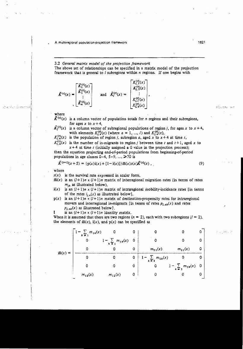
3.2 General malrix model of the projection framework The above set of relationships can be specified in a matrix model of the projection framework that is general to I subregions within n regions. If one begins with

and ir(x) = K(1l(x)/.1 K(r)(x)1.0

where i(r)(x) is a column vector of population totals for n regions and their subregions,

for ages x to x+4, is a column vector of subregional populations of region j. for ages x to x +4, with elements Klr~(x) (where a = I, ... , 1) and K/~fJ(X),

Kft)(x)/. G is the population of region j, subregion a, aged x to x +4 at time t.

K(r)(x)1.0 is the number of in-migrants to region j between time I and I + I, aged x to

x+4 at time t (initially assigned a 0 value in the projection process); then the equation projecting end-of-period populations from beginning-of-period populations in age classes 0-4, 5-9, ... , ;>70 is

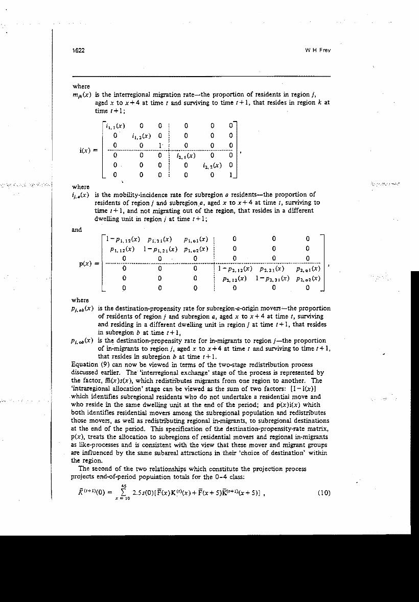
i(t·+-!)(x+ 5) = (p(x)i(x) + [I - i(x)l} m(x)s(x)K (t)(x) , (9)

where sex) is the survival rate expressed in scalar fonn, m(x) is an (/+ l)n x (/+ l)n matrix of interregional migration rates (in tenns of rates

mik as illustrated below), i(x) is an (1+ l)n x (1+ l)n matrix of intraregional mobility-incidence rates [in terms

of the rates ii. a(x) as illustrated below 1, pCx) is an (1+ l)n x (1+ l)n matrix of destination-propensity rates for intraregional

movers and interregional in-migrants [in terms of rates Pi,ab(X) and rates PI,Ob(X) as illustrated below],

I is an (1+ l)n x (l + l)n identity matrix. When it is assumed that there are two regions (n = 2), each with two subregions 1.1 = 2), the elements of m(x), i(x), and p(x) can be specified as

1- I ma(X) o o o o o k .. I

o 1- I mlk(X) 0 o o o k .. 1

oo o o iii(x) = ···-······~··············-··..··..~········..······~-T..;·:···I···~·~:(~)·....···..···O····....··..··~

Ie .. 2

o o o o I - I m'lk(x) 0 Ie .. :1

o o o o

1622 W H Frey

where m,7c(x) is the interregional migration rate-the proportion of residents in region j,

aged x to x +4 at time t and surviving to time t + 1, that resides in region k at time t+ 1;

il,I(X) 0 0 0 0 0

0 i l ,2(X) 0 0 0 0 0 0 I' 0 0 0 ............................... "' ............................-.. -............... ......-."'......... -- ...----_ ........~ ,i(x) = 0 0 0 i2, I(x) 0 0 0 0 0 0 i:,2(X) 0 0 0 0 0 0

where ii ... (x) is the mobility-incidence rate for subregion a residents-the proportion of

residents of region j and subregion,a, aged x to x+ 4 at time t, surviving to time t+ 1, and not migrating out of the region, that resides in a different d welling unit in region j at time t + 1 ;

and

I-Pl,12(X) PI;2I(X) Pl,Ol(X) 0 0 0

Pl,I2(X) I-PI,H(X) Pl.o2(X) 0 0 0 0 0 0 0 0 0

.............. " .................................................................... "'.............. _ ..........}_................ a ....................."' ........................................ ,;0"............p(x) = 0 0 0 1- P2,12(X) P2,21 (x) P2,oI (x)

0 0 0 P2.12(X) 1-P2,21 (x) Pl,02(X)

0 0 0 0 0 0

where Pi...b(X) is the destination-propensity rate for subregion-a-origin movers'-the proportion

of residents of region j and subregion a, aged x to x+ 4 at time t, surviving and residing in a different dwelling unit in region j at time r+ 1, that resides in subregion b at time t + 1,

Pi,ob(X) is th~ destination-propensity rate for in-migrants to region j-the proportion of in-migrants to region i, aged x to x+4 at time r and surviving to time t+ 1, that resides in subregion b at time t + 1.

Equation (9) can now be viewed in tenns of the two-stage redistdbution process discussed earlier. The 'interregional exchange' stage of the process is represented by the factor, ii'i(x)s(x), which redistributes migrants from one region to another. The 'intraregional allocation' stage can be viewed as the sum of two factors: [I-i(x)] which identifies subregional residents who do not undertake a residential move and who reside in the same dwelling unit at the end of the period; and p(x)i(x) which both identifies residential movers among the subregional population and redistributes those movers, as well as redistributing regional in-migrants, to subregional destinations at the end of the period. This specification of the destination-propensity-rate matrix, p(x), treats the allocation to subregions of residential movers and regional in-migrants as like-processes and is consistent with the view that these mover and migrant groups are influenced by the same sub areal attractions in their 'choice of destination' within the region.

The second of the two relationships which constitute the projection process projects end-of-period population totals for the 0-4 class:

4S

i(1+I)(O) = L 2.5s(O)[F\x)K(t)(x)+F(x+ 5)K<t+l)(X+ 5)] , (10) x= lO

A multiregional population'projection framework 1623

where s(O) is the survival rate of births expressed in scalar terms [as in equations (2), (5),

and (6)], F(x) is an (/ +1 ) n x (l+ l)n matrix of fertility rates [specified below in terms of

elements fi(x)]. When it is assumed that the subregions of each region will exhibit the same fertility rates as the region, the F(x) matrix for an illustrative two-region model is specified as follows:

flex) 0 0 0 0 0 , 0 flex) 0 0 0 0

0 0 0 0 0 0.....•...........•.."" ...,..........................F(x) = 0 0 0 flex) 0 0

0 0 0 0 hex) 0

0 0 0 0 0 0

where fi(x) is the fertility rate-the average annual number of births to persons aged x to

x+ 4 in region j. The reader should note that, although the framework outlined in relationships (9)

and (10) can handle up to I subregions within each region, the number of subregions can vary across regions, and there need not be any subregions in one or more regions. In the first instance, only relevant subareas should be given initial year (t = I) populations in submatrix Kit)(x) for the region, with all other i./~~(X) elements given a value of O. In the second instance, the initial year population of the total region should be inserted in the Kr~(x) element, with all other elements given a value of O. For both instances, appropriate changes need to be made within the m(x), p(x), and i(x) matrices. Taken together, relationships (9) and (10) constitute a more general model of the two-stage interregional and intraregional projection-process than was specified for the particular example of intrametropolitan city-suburban redistribution earlier in this section. Because the end-of-period matrix j{(r+l)(x) for ages 5-9, 10-14, ... , represents the begin.n.ing-of-period matrix j{(t)(x) for the subsequent projection-period, these relationships can produce projected population sizes for I subregions within n regions for any desired number of periods.

3.3 Rate calculation and data considerations An important feature of the two-stage projection-process is its relatively parsimonious data requirements for estimation of mobility rates. If the conventional 'single-stage' multiregional methodology were adapted to accommodate projections of I subregions within n regions, the number of new 'regions' would simply be expanded to In and it would be necessary to compile a nationwide origin-destination matrix of In x In movement flows to estimate the movement rates for the projection framework.

The two-stage model requires only a nationwide origin-destination matrix of n x n flows, and an I x I origin-destination matrix for each region (or for those regions where a subregion projection is desired). In a nation of five regions with two subregions each. the flfst methodology would require a lOx 10 nationwide-flow matrix, and the second methodology would require a 5 x 5 nationwide matrix and a 2 x 2 matrix for each of the five subregions. The latter, more compact nationwide-flow matrix is advantageous for rate estimation, because it is likely to yield far fewer sparsely populated flows than would be the case with the full-scale nationwide subregion-to-subregion matrix.

The basic migration and mobility parameters that are required for matrix relationship (9) [or for equations (1), (3), (4), (7), and (8) in the specific city-suburb

'j ;.::~~ i:·:\>:j.\;".- .....:.'.

1624 W H Frey

example] are: mile for origin region j and destination region k U, k = 1,2, "', n); i j•1H Pj••b, and Pi.ob for up to I subregions, a, b, within one or more of the n regions. With the assumption that the period t to t + 1 is equal to the age-category interval (five years in this case), all of these rates can be estimated from the following flXed­interval migration tabulations that are available from a census: labulation A nationwide population aged :>5, cross tabulated by region of residence, region of residence five years ago, and five-year age groups; tabulation B regional population (for each region of interest), aged :>5, cross tabulated by residence in same or different dwelling unit as five years ago, subregion of residence (within the region) five years ago, and five-year age categories(7). The rates are computed as follows:

region k residents, aged x + 5 to x + 9 at census, who resided in region j, five years ago . aU' national residents aged x + 5 to x + 9 at census, ' who resided in region j, five years ago

all region j residents, aged x + 5 to x + 9 at census, who lived in a different dwelling unit located in subregion a of that region, five years ago

ii•• (x) = all region j residents, aged x + 5 to x + 9 at census, who resided in the same or different dwelling unit in subregion a of that region, five years ago

subregion b, region j residents, aged x+ 5 to x+ 9 at census, who lived in a different dwelling unit located in subregion a of that region, five years ago

Pi,flbCx) = -----...;:;...--------''''---'---'---~ all region j residents, aged x + 5 to x +9 at census, who lived in a different dwelling unit located in subregion a of that region, five years ago

subregion b, region j residents, aged x + 5 to x + 9 at census, who lived in a different dwelling unit

. (x) = located outside the region j, five years ago . hob all region j residents, aged x + 5 to x + 9 at census,

who lived in a different dwelling unit outside region j, five years ago

The survival and fertility parameters, s(x) and f;(x), required for matrix relationships (9) and (10) [or equations (2), (5), and (6) in the specific city-suburb example] can be computed in a more straightforward fashion with available vital statistics data and census tabulations, using standard techniques (Shryock and Siegel, 1971; Rogers, 1975).

Notice that only the nationwide tabulation A is necessary to compute the mjle(x) interregional migration rates needed to construct matrix ffi(x) in . equation (9). Only region-specific tabulations B are necessary to compute the incidence rates ii••(x) and and propensity rates P"fI.b(x) and PI.Ob(X) needed for matrices i(x) and p(x). It should now be clear why movement-rate estimation becomes simplified when it is assumed

(7) Some data sources do not distinguish between same and different dwelling,unit residences for individuals that do not move across subregion boundaries. This precludes estimation of separate mobility·incidence rates and destination-propensity rates for residential movers in equation (9). An alternative specification for such data sources is offered in the appendix to the paper by Long and Frey (198,2).

1625A multiregional population-projection framework

that (I) all subregional residents in a given region exhibit the same age-specific out­migration rates [as in equation (8) in section 3.1, or in ffi(x) in section 3.2}; and (2) intraregional mobility-incidence rates are conditional on residents not migrating out of the region [as defmed in equations (3) and (4) in section 3.1; and in matrix i(x) of section 3.2]. If assumption (1) were not made, then it would be necessary to tabulate a nationwide In x n origin-destination migration matrix to compute all

. mlk(x). Likewise, if assumption (2) were not made, the same matrix-in addition to tabulation B-would be necessary to compute all ii, b(x)'

An important feature of this projection framework is its capability to produce 'updated' projections when current, but limited, data become available. For example, assume that equations (9) and (10) were employed to produce intraregional and inter­regional projections on the basis of fixed-interval migration tabulations A and B that were available with the past census. Several years after the census is taken, a comprehen,sive survey of residents in one region j becomes available, which includes appropriate information to compile a current tabulation B .. TIlls allows the researcher to produce an 'updated' projection of subregions within region i based on the same interregional migration, fertility, and mortality parameters [ffl(x), sex), ''(x)] as the last projections, but based on more current intraregional allocation parameters for region j [i,..,ex), Pi,/J(x), PI,ob(X)].

In this vein, it should be noted from the above that the destination-propensity rates, PI, db (x) and PI,ob(x) needed for the p(x) matrix in equation (9) can be computed from a survey of the movers in a region. Thus, the availability of a ,,'urrent survey of movers provides the capability of updating past projections, if one is willing to assume that the previous i/,/J(x) rates, in addition to the previous mlk(x), sex), and ''(x) rates, hold for the current update. Because age-specific incidence rates tend to vary less across time and space than destination-propensity rates and because the latter are directly linked to the intraregional mover and migrant allocation-process (Frey, 1978b; 1979b), an updating of intraregional projections on the basis of current destination-propensity rates constitutes an inexpensive means of compiling timely projections between censuses.

4 Application to three US metropolitan areas 4.1 Baseline projections from 1970 census data The projection framework outlined in the previous section will be employed to project intrametropolitan central-city-suburban redistribution for three large SMSAs­Detroit, Atlanta, and Houston. The largest US SMSAs are generally recognized to be self-contained labor-market regions, and have been included as such both in the Bureau of Economic Analysis and in the State Economic area-regionalization schemes (II) • The three SMSAs selected for this application display distinctly different core­periphery and metropolitan-wide population change patterns over the base period for the projection 1965 -1970. Detroit represents a declining industrial metropolis that has sustained considerable city loss and core-periphery decentralization; Atlanta is a growing SMSA, although also undergoing a significant intrametropolitan city-suburb redistribution; Houston, growing faster than Atlanta or Detroit, registers moderate growth in its central city as a consequence of a much less pronounced decentralization process.

(8) These constitute alternative regionalizations of the national territory wherein the regions approximate single labor-market areas. The 183 Bureau of Economic Analysis Areas, designated by the Bureau of Economic Analysis, approximate self-contained commuting regions based on the nodal functional concept [see discussion in Hall and Hay 0980, pages 3-14]. The 510 State Economic Areas designated by the US Bureau of the Census (1970) represent groups of counties that are homogeneous with respect to social and economic characteristics.

1626 W H Frey

For simplicity of exposition, the interregional and intraregional projections to be undertaken for each SMSA will be based on a simple two-region system where one region consists of the SMSA of interest, and the other region consists of the 'rest of the USA'. The intraregional projection will then occur within the SMSA region­across the central-city and suburban 'subregions' of the SMSA. nus simplified regional system therefore requires that a separate projection analysis be undertaken for each SMSA. (A more elaborate analysis would include all national labor-market areas-including the three SMSAs-m the regional scheme, and would require only one projection analysis.) The projection process is consistent with equations (1 )-(8) which are tailored to the specific case of city-suburb redistribution where there are two regions (11 = :!), such that j = I for the SMSA of interest and j = 2 for the rest of the country. Alternatively, the more general specifications in relationships (9) and (10) also apply where 11 = 2 and I = 2 in region I, such that a and b can be designated as c or s (for central city or suburbs) in the SMSA of interest.

Appropriate fiied-interval migration data are available from special tabulations from the 1970 US census and from the US Bureau of the Census (1973). These data make it possible to derive tabulation A to compute the interregional exchange rates [mI2(x) and 111 2 I (x) J ; "and tabulation B to compute the intraregional allocation rates [ii. ~(x), ii. s (x), Pi. os (x), Pi. ,o(x). Pi, oc(x), Pi. os (x )]. The census tabulations were adjusted for a mover's unknown residence five years prior to the census by allocating 'unknowns' to locations appropriate to individuals with similar race, age, and socioeconomic characteristics. The tabulations were also adjusted for census underenumeration using measures developed by the US Bureau of the Census (19 77b). The 1965-1970 migration and residential mobility parameters for the Detroit SMSA are shown in table:!. In these projections, nationwide age-specific survival rates (s(x)] and nation­wide age-specific fertility rates [h(x)] are assumed to hold for all regions and periods.

Table 2. Migration and residential mobility parameters for Detroit SMSA, based on 1965-1970 period (source: 1970 US Census tabulations adjusted for 'residence five years ago not known' and census underenumeration). The symbolic parameters are explained in the text.

Age at SMSA Surviving Mobility·incidence Destination-propensity rates of start of out· in·migrants rates of

city- suburb- in-migrants to period, migration to SMSA city suburb origin origin SMSAx tox-t4 rate residents residents movers movers

/I /I

k mjk(x) k s{x)iQflmkix) ii.~(x) ii,s(x) Pi.cs(x) PI•.J.x ) Pi. oJx) Pi. os(x)k=lk=1 b,. r k'¢j

0-4 0.1054 45988 0.5910 0.3755 0.3165 0.0796 0.3520 0.6480 5-9 0.0820 31505 0.4749 0.2712 0.2956 0.0775 0.3004 0.6996

10-14 0.1264 24915 0.4294 0.2504 0.2780 0.1044 0.3731 0.6269 15-19 0.2215 54:!33 0.6509 0.6018 0.2888 0.1353 0.40?:! 0.5928 20-24 0.1513 61445 0.7713 0.6774 0.3808 0.1062 0.3515 0.6485 25-29 0.1267 31351 0.6644 0.4736 0.3680 0.0899 0.3353 0.6647 30-34 0.0878 20542 0.5372 0.3494 0.3269 0.0804 0.3329 0.6671 35-39 0.0870 16431 0.4467 0.2430 0.3314 0.0939 0.2465 0.7535 40-44 0.0552 12179 0.3692 0.2097 0.3304 0.0913 0.2651 0.7349 45-49 0.0540 8487 0.3429 0.2078 03613 0.1195 0.3492 0.6508 50-54 0.0774 4924 0.31:22 0.1959 0.3772 0.1336 0.3635 0.6365 55-59 0.073,5 3902 0.3059 0.1876 03430 0.1105 0.3810 0.6140 60-64 0.0983 3253 0.2838 0.1896 0.4002 0.1363 0.4644 0.5356 65-69 0.0904 2728 0.2761 0.2043 0.3060 0.13:25 0.3658 0.6342 >70 0.0874 6043 0.3084 0.2304 0.3683 0.2058 0.3867 0.6133

1627A multiregional population-projection framework

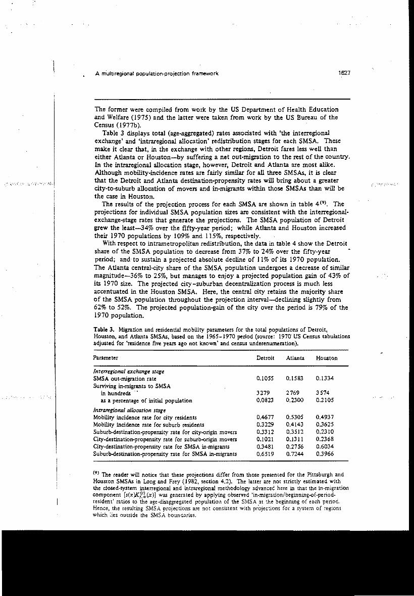
The former were compiled from work by the US Department of Health Education and Welfare (1975) and the latter were taken from work by the US Bureau of the Census (1977b).

Table 3 displays total (age-aggregated) rates associated with 'the interregional exchange' and 'intraregional allocation' redistribution stages for each SMSA. These make it clear that, in the exchange with other regions, Detroit fares less well than either Atlanta or Houston-by suffering a net out-migration to the rest of the country. In the intra.regional allocation stage, however, Detroit and Atlanta are most alike. Although mobility-incidence rates are fairly similar for all three SMSAs, it is clear that the Detroit and Atlanta destination-propensity rates will bring about a greater city-to-suburb allocation of movers and in-migrants within those SMSAs than will be the case in Houston.

The results of the projection process for each SMSA are shown in table 4(9). The projections for individual SMSA population sizes are consistent with the interregional­exchange-stage rates that generate the projections. The SMSA population of Detroit grew the least-34% over the fifty-year period; while Atlanta and Houston incre;lSed their 1970 populations by 109% and 115%, respectively.

With respect to intrametropolitan redistribution, the data in table 4 show the Detroit share of the SMSA population to decrease from 37% to 24% over the fifty-year period; and to sustain a projected absolute decline of 11% of its 1970 population. The Atlanta central-city share of the SMSA population undergoes a decrease of similar magnitude-36% to 25%, but manages to enjoy a projected population gain of 43% of its 1970 size. The projected city-suburban decentralization process is much less accentuated in the Houston SMSA. Here, the central city retains the majority share of the SMSA population throughout the projection interval-declining slightly from 62% to 52%. The projected population-gain of the city over the period is 79% of the 1970 population.

Table 3. Migration and residential mobility parameters for the total populations of Detroit, Houston. and Atlanta SMSAs, based on the 1965 -1970 period (source: 1970· US Census tabulations adjusted for 'residence five years ago not known' and census underenumeration).

Parameter Detroit Atlanta Houston

Interregional excJumge stage SMSA out-migration rate 0.1055 0.1583 0.1334 SUrviving in-migrants to SMSA

in hundreds .. 3279 2769 3574 as a percentage of initial population 0.0823 0.2300 0.2105

Inrrarr:gional allocation stage Mobility incidence rate for city residents 0.4677 0.5305 0.4937 Mobility incidence rate for suburb residents 0.3229 0.4143 0.3625 Suburb-destination-propensity rate for city-origin movers 0.3312 0.3512 0.2310 City.destination-propensity rate for suburb-origin movers 0.1021 0.1311 0.2368 City-destination-propensity rate for SMSA in-migrants 0.3481 0.2756 0.6034 Suburb-destination-propensity rate for SMSA in-migrants 0.6519 0.7244 0.3966

(9) The reader will notice that these projections differ from those presented for the Pittsburgh and Houston SMSAs in Long and Frey (1982, section 4.2). The latter are not strictly estimated with the closed-system interregional and irmaregional methodology advanced here in that the in-migration component [s(x)K?b(x)] was generated by applying observed 'in·migration/beginning-of.period­resident' ratios to the age-disaggregated populatio,l of the SMSA at the beginning of each period. Hence, the resulting SMSA projections are not consistent with projections for a system of regions which lies outside the SMSA boundaries.

.» '.,<, ...•'.:

1628 W H Frey

Table 5 provides insights into how the migration, residential mobility, and natural increase components of change contribute to the city-suburb redistribution process of each SMSA over the fifty-year projection-period. The data parallel those presented for the base period in table 1. Again, each SMSA undergoes a significant projected city-to-suburb redistribution as a result of the intrametropolitan residential mobility

Table 4. Projected population sizes and city and suburb shares of the population, for 1970-2020 for Detroit, Atlanta, and Houston SMSAs (source: projection equations (1)-(8) in text; with all input populations and rates from 1970 US Census tabulations adjusted for 'residence five years ago not known' and census underenumeration].

Population size and Year city and suburb shares

1970 1980 1990 2000 2010 2020

Derroit SMSA . \

Total size (in thousands) Population share (%)

city suburb

. 4328

36.6 63.4

4570

30.3 69.7

4899

27;0 73.0

5171

25.3 74.7

5485

24.6 75.4

5798

24.3 75.7

AtiD:nca SMSA Total sIZe (in thousands) Population share (%)

city suburb

}437

36.4 63.6

1795

29.5 70.5

2148

26.6 73.4

2448

25.4 74.6

2737

25.1 74.9

2998

25.0 75.0

Houston SMSA Total size (in thousands) Population share (%)

city suburb

2048

62.3 37.7

2566

57.1 42.9

3097

54.2 45.8

3551

52.8 47.2

3991

52.3 47.7

4396

51.9 48.1

Table 5. Contributions to projected central-city, suburb, and SMSA population change, for 1970- 2020 attributable to natural increase, net migration, and net intrarnetropolitan residential mobility for DetrOit, Atlanta, and Houston SMSAs [source: projection equations (l )-(8) in text; with all input populations and rates from US Census tabulations adjusted for 'residence five years ago not known' and census underenumerationj.

Projected population Detroit Atlanta Houston size and projected components of change central

city suburbs SMSA central

city su burbs SMSA . central

city suburbs SMSA

Projected 2020 popuiD:tion size (in thousands) 1407 4390 5797 748 2250 2998 2280 2116 4396

Components of 1970- 2020 popuiD:tio" change a (as percent of 2020 population size) Natural increase 43.5 38.3 39.6 46.7 41.4 42.7 43.8 36.0 40.1 Net migration

and mobility -56.0 -0.9 -14.2 -16.6 18.0 9.4 0.2 27.4 13.4 Net migration

to outside SMSA 4.2 -20.2 -14.2 10.7 8.9 9.4 25.2· 0.5 13.4 Net mobility

within SMSA -60.2 19.3 -27.3 9.1 -25.0 26.9

a The contribution to 1970-2020 population change attributable to each component (that is, natural increase, net migration, net mobility) is calculated by summing the contribution of that component to population change during each period, 19.70-1975, ... , 2015-2020, over the ten five-year periods of the projection span. TIlls sum of period contribution is then expressed as a percentage of the projected 2020 population size of the appropriate area (that is, central City, suburb, SMSA).

.' "" " ",' "" ~ "" ..,. -.. ". ,"

1629A mu/tiregional population-projection framework

streams. However, this redistribution is 'cushioned' in Atlanta and Houston as a result of net in-migration to the SMSA as a. whole-and to city and suburb subregions. The data show clearly that the prospects of long-tenn population gains for all subregions in a labor-market area are enhanced when the labor market, as a whole,· sustains a. constant net in-migration vis-a-vis other labor markets.

4.2 'Updating' the projections with post-census survey data . As indicated in section 3.3, the projection framework advanced here provides the capability for updating projections when recent, more limited mobility-tabulations become available for single regions in the regional system. Large-scale post-1970 surveys of movers in the Detroit, Atlanta, and Houston SMSAs provide the opportunity to perfonn updates to the 'baseline' 1970 census-based projections presented above. These updated projections will assume the same rates for interregional migration,

\

mobility incidence, survival, and fertility as did the baseline projections. However, their destination-propensity rates (PI. C$' PI, Ie, PI. oc' and PI. OIS) will be calculated from the survey data collected in the late 1 970s. The survey tabulations that are used to estimate the late 1970s destination-propensity rates are compiled from the metropolitan area-wide Annual Housing Surveys undertaken in the Atlanta, Houston, and Detroit SMSAs in 1975, 1976, and 1977, respectively [as discussed by US Bureau of the Census (l977a; 1978; 1980)J. Approximately 15000 households are interviewed in each SMSA survey, which ascertains the number and ages of household members, and if the household (head) has changed residence over the previous year, and the locatiort of the previous residence, whether in city or suburb or outside the SMSA. The post­1970 destination-propensity rates used in updating the 1970 census-based projections for each SMSA were calculated from a tabulation of mover-household members(10).

Figure 1 provides some indication of how age-specific destination-propensity rates for the late 1970s, to be used in the updated projections, differ from those for the late I 960s. Because of the limited sample size of the Annual Housing Survey, it is necessary to collapse age categories into end-of-period values: 5-14, 15-24,25-34, 35-44,45-54, and ;>55. Late 1970s and late 1960s rates are both presented in this manner to facilitate comparisons. In general, there is a tendency toward increased city-to-suburb redistribution. All three SMSAs show lower city-destination-propensity rates both for suburban-origin movers and for metropolitan in-migrants in the late 19705 than in the late 1960s [figures l(b) and l(c)]. Further, Atlanta shows a significant increase in its suburb destination-propensity-rate for city-origin movers [figure 1 (a) J. This tendency is not exhibited for either Detroit or Houston.

The updated intrametropolitan projections for· the three SMSAs can be contrasted with the baseline projections in figure 2. Both sets of projections begin with 1970, and progress through ten five-year periods to the year 2020. They differ only in the destination-propensity rates that are assumed. Hence, these comparisons provide a means of evaluating the long-tenn redistribution implications of changes in intra­metropolitan destination selections by movers and migrants in the late 19705, when all other migration, mortality, and fertility assumptions are' held constant.

(10) For each metropolitan area, a tabulation was prepared for members of households whose head moved during the year preceding the survey. The tabulations cross-classified the city and suburb location at the date of the survey by city, suburb, or outside the SMSA locations of previOUS . residence for household members in age classes 5-14,15-24,25-34,35-44,45-54, and ;>55 at the time of the survey. Hence. the destination-propensity rates compiled from these data are based on mobility observations over a one-year (not five-year) period and pertain to the end-of-period household population (not total population) in each SMSA. In generating the projections, destination­propensity rates for five-year age-class mUltiples (that is, 5-14) are applied to each five-year age group in the class (for example, 5-9 and 10-14).

1630 W H Frey

It is clear from the plots that the more recently registered destination-propensity rates will provide a more significant city-to-suburb redistribution of population in all three SMSAs, than would have occurred on the basis of late 1960 rates. The updated projections show that the share of SMSA population living in the central city of Detroit will fall to 18%, as contrasted with the 24% share with the baseline projections. The newly projected central-city share for Atlanta for the year 2020 is only 12% as contrasted with the previously projected 25% share. The central city and suburbs of Houston will grow rapidly under each projection. However, the 'updated' projection no longer shows the central city to dominate the suburbs throughout the projection period. By the year 1990, the suburbs of Houston are now projected to overtake the central city.

Although the updated projections represent something of a compromise between older projection~, wherein all rates were calculated from data for the same base­period, and the need to produce equally elaborate projections from the current year, they do constitute a means to assess the aggregate implications of intercensal movement-patterns until a more satisfactory data base becomes available with the

0.6

O.S

0.4

;;" 0.3ex: 0.2

0.1

0.0 (a)

0.3

;;" 0.204~ex: 0.1

0.0 (b)

0.6"j0.5

0.4 ~ .." ex: 0.3

! 0.2

0.1

0.0 (e)

Detroit Atlanta

, I

J

~ I , J

--II "

Detroit Atlanta

~~ ! ---- ........ '

i i j , i J

Detroit

,,"\ ,,',-

\ I ,,' ,

Age group

i I I I j (

Atlanta

o ( I/",~~/, I ", "

I v'"

Iii t i

Age group

Howton

Houston

~.. ,.... ,,-­

Houston

~ J '" I " I

Age group

Figure 1. Mover and in'migrant destination-propensity rates for the late 1960$ (solid lines) and late 1970s (dotted lines): (a) suburb destination-propensity rates for eity-origin movers, (b) city.destinl!tion­propensity rates for suburb-origin movers, (c) city.destination.propensity rates for SMSA in-migrants. (Note: Rate is defmed as the proportion ofa residents of an area, aged x to x+ 4 at time r, who survive and live in another area Or in a different dwelling unit in the same area at time r+ 1.)

.~:. .,".",',' ~",

1631A multiregional population-projection framework

next census. The 'updated' projections above, for example, serve to counter a popularly held view that a significant 'return to the city' had occurred in large metropolitan areas since the 1970 census was taken.

Detroit Atlanta Houston 250

,+ suburbs ,;-,+ 1970s __ +,+'

400

150500

2001960. -=--t." 200 ,+

,:,·.,.t:t.•»",,;,-'\ ,t ­

s ISO 1508 300

0 ::. c 0 central city <:en nal city

100:; 200 100 1970s

Q, " ,f ...,.~+196~S '\ .~ .... -+-,.........-+-t100 50 50 ~

~+..._+..,..:.+-r

0 1980 2000 2020 1980 2000 2020 1980 2000 2020

0 0

Yea: Yea: Yea:

Figure 2. Alternative projections of city and suburb population sizes, for 1970-2020 based on assumptions of late 1960$ and late 19705 destination-propensity rates for Detroit, Atlanta, and Houston SMSAs.

S Conclusion I have introduced in this paper a population-projection framework that incorporates both interregional migration and intraregional residential mobility streams to project future population sizes both across and within regions in a manner that is consistent with existing muitiregional migration theory. I have also shown how the framework can be operationalized with fLXed-interval migration data that a.re commonly available from censuses and surveys. A significant advantage of this framework over the existing muitiregional projection methodology is its parsimonious data requirements when both interregional and intraregional projections are desired. It also pennits the user to 'update' baseline projections when recent, more limited regional survey data become available. These features of the framework were demonstrated through projections of. intrametropolitan central-city-suburban redistribution for three US SMSAs based on migration data from the 1970 US Census and metropolitan area-wide Annual Housing Surveys undertaken in each SMSA over the 1975-1977 period. Although this inter/ intraregional projection-framework can be employed with any regionalization scheme the user desires, it is most consistent with underlying migration and residential mobility processes when the 'regions' correspond to self-contained labor-market areas such as Standard Metropolitan Statistical Areas or Bureau of Economic Analysis Areas in the United States of America, or Metropolitan Economic Labor Areas in the United Kingdom.

Acknowledgements. The author wishes to acknowledge the helpful suggestiOns of Luis Castro, Jacques Ledent. Kao-Lee Liaw, Dimiter Philipov, Philip Rees, Andrei Rogers, and Frans Wille kens. He also thanks Mark L Langberg for help with reviSing an earlier draft of the manuscript and Michael Coble, Cheryl Knobeloch and Frank Nieder for computer assistance rendered.

This research is supported by research grant number ROI HDI658I, "Migration and Redistribution: SMSA Determinants" from the Center for Population Research of the National Institute of Child Health and Human Development and was initiated during the author's tenure as a visiting Research Scholar at the InterT'13flnn'1! Tn(;tit11l'P (("'It" ,\ ••" ..... ;;".,.-1 '''no .......... \ ... .,1.,,,;,.. T _"."_t",_~ " ."'...,1"> .?"< ..... ,

1632 W H Frey

Rererences Frey W H, 1978a, "Black movement to the suburbs: potentials and prospects of metropolitan-wide

integration" in The Demography of Racial and Ethnic Groups Eds F D Bean, WP Frisbie (Academic Press, New York) pp 79-117

Frey W H, 1978b, "Population movement and city-suburb redistribution: an analytic framework" Demography 15(4) 571-588

Frey W H. 1979a, "Central city white flight: racial and nonracial causes" Ameriam SociologiCilI Review 44(3) 425-448

Frey W H, 1979b. "White flight and central city loss: application of an analytic migration framework" Environment and Planning A 11 129-147

Frey W H, 1983. "Ufecourse migration of metropolitan whites and blacks and the structure of demographic chatlge in large central cities" DP-83-47, The Population Studies Center of the University of Michigan, Ann Arbor. MI

Goodman J L Jr, 1978 Urban Residential Mobility: Places, People and Policy The Urban Institute, Washington, DC

Greenwood M J, 1975. "Research on internal migration in the United States: a survey" Joumt11 of Economic Literature 13 397 -433

Greenwood M J, 1981 Migration and Economic Growth in the US: National Regional and Metropolitan Perspectives (Academic Press, New York)

Hall P, Hay D, 1980 Growth Centres in the European Urban System (Heinemann, London) lansing J R, Mueller E, 1967, "The geographic mobility oflabor" Institute for Social Research,

University of Michigan, Ann Arbor, MI Long L H, 1973, "New estimates of migration expectancy in the United States" J0Umt11 of the

American Statistical Association 6837-43 Long L H, Frey W H, 1982, "Migration and settlement: 14. United States" RR-82-15, International

Institute for Applied Systems Analysis, Laxenburg, AuStria Lowry 1 S, 1966 Migration and Metropolitan Growth (Chandler, San Francisco, CAl Morrison P A, 1972, "Population movements and the shape of urban growth: implications for

public policy" in Population Distribution and Policy Ed. S M Mazie, volume V of research reports of US COmmission on Population Growth and the American Future (US Government Printing Office, Washington, DC) pp 281-322

Rees P H, Wilson A G, 1977 Spatial Population AnalysiS (Edward Arnold, London) Rogers A, 19751ntroduction to Mulriregional Mathematical Demography (John Wiley, New York) Rossi P H, 1955 Why Families Move (Free Press, New York) Shryock H S, Siegel J S, 1971 The Methods and Materials of Demography (US Government Printing

Office, Washington, DC) Speare A Jr, Goldstein S, Frey W H, 1975 Residential Mobility, Migration and Metropolitan Ouznge

(Ballinger, Cambridge, MA) US Bureau of the Census, 19701970 Census User's Guide (US Government Printing Office,

Washington, DC) US Bureau of. the Census, 1973 Census of Population 1970. Subject Reports. Final Repon

PQ2)-C Mobility for Metropoliran Areas (US Government Printing Office, Washington, DC) US Bureau of .the Census, 1977a Cu"ent Housing Reports H-170-75-21. Annual Housing Survey:

1975. Atiama, Georgia SMSA (US Government Printing Office, Washington, DC) · 1 US Bureau of the Census, 1977b ProjectionJ of the Population of the United States, 1977 to 2050.

Current Population Reports. Series P-25. number 704 (US Government Printing Office, Washington, DC)

US Bureau of the Census, 1978 Current Housing Repom H-17()" 76-49. Annual Housing Survey: 1976: Houston, Texas SMSA. (US Government Printing Office, Washington, DC)

US Bureau of the Census, 1980 Cu"ent Housing Reports H-170-77-5. Annual Housing Survey: 1977. Detroit. Michigan SMSA (US Government Printing Office, Washington, DC)

US Department of Health Education and Welfare, 1975 US Decennial Life Tables for 1969-71. Volume 1 number 1, DHEW Publication number (HRA) 75-1150 (US Government Printing Office, Washington, DC)

Willekens F, Rogers A, 1978, "Spatial population analysis: methods and computer programs" RR· 78-18, International Institute for Applied Systems Analysis, Laxenburg, Austria

p © 1983 a Pion DublicaT,on orin!ed in Gre?T RriTilin

.; .•.•\.::; 1:'" .~,