Embed Size (px)
Citation preview
arX
iv:2
104.
0585
4v2
[he
p-ph
] 2
1 Ju
n 20
21
EPJ manuscript No.(will be inserted by the editor)
QCD phase diagram in a magnetized medium from the chiralsymmetry perspective: The linear sigma model with quarks andthe Nambu–Jona-Lasinio model effective descriptions
Alejandro Ayala1,2, Luis A. Hernandez3,2, Marcelo Loewe4,5,2, and Cristian Villavicencio6
1 Instituto de Ciencias Nucleares, Universidad Nacional Autonoma de Mexico, Apartado Postal 70-543, CdMx 04510, Mexico.2 Centre for Theoretical and Mathematical Physics, and Department of Physics, University of Cape Town, Rondebosch 7700,South Africa.
3 Departamento de Fısica, Universidad Autonoma Metropolitana-Iztapalapa, Av. San Rafael Atlixco 186, CdMx 09340, Mexico.4 Instituto de Fısica, Pontificia Universidad Catolica de Chile, Casilla 306, Santiago, Chile.5 Centro Cientıfico Tecnologico de Valparaıso-CCTVAL, Universidad Tecnica Federico Santa Marıa, Casilla 110-V, Valparaıso,Chile.
6 Centro de Ciencias Exactas and Departamento de Ciencias Basicas, Facultad de Ciencias, Universidad del Bıo-Bıo, Casilla447, Chillan, Chile.
Received: date / Revised version: date
Abstract We review the main features of the QCD phase diagram description, at finite temperature,baryon density and in the presence of a magnetic field, from the point of view of effective models, whosemain ingredient is chiral symmetry. We concentrate our attention on two of these models: The linear sigmamodel with quarks and the Nambu–Jona-Lasinio model. We show that a main ingredient to understand thecharacteristics of the phase transitions is the inclusion of plasma screening effects that capture the physicsof collective, long-wave modes, and thus describe a prime property of plasmas near transition lines, namely,long distance correlations. Inclusion of plasma screening makes possible to understand the inverse magneticcatalysis phenomenon even without the need to consider magnetic field-dependent coupling constants.Screening is also responsible for the emergence of a critical end point in the phase diagram even for smallmagnetic field strengths. Although versatile, the NJL model is also a more limited approach since, beinga non-renormalizable model, a clear separation between pure vacuum and medium effects is not alwayspossible. The model cannot describe inverse magnetic catalysis unless a magnetic field dependent couplingis included. The location of the critical end point strongly depends on the choice of the type of interactionand on the magnetic field dependence of the corresponding coupling. Overall, both models provide sensibletools to explore the properties of magnetized, strongly interacting matter. However, a cross talk amongthem as well as a consistent physical approach to determine the model parameters is much needed.
1 Introduction
The study of the different phases that strongly interact-ing matter can reach when varying control parameters,such as temperature, baryon and isospin density, etc., isnowadays one of the most active fields at the crossroads ofnuclear and particle physics. The interest grew with therecent lattice QCD (LQCD) discovery of the inverse mag-netic catalysis (IMC) phenomenon, whereby the criticaltemperature for the chiral symmetry restoration transi-tion decreases as a function of the strength of another ofthe control parameters, an external magnetic field [1,2,3]. This discovery has prompeted research on the proper-ties of the so called magnetized QCD phase diagram. Inaddition, the recent successful detection of gravitationalwaves [4] from a binary neutron star merger, has kickedoff the era of multi-messenger physics to study stronglyinteracting systems. The information obtained by study-
ing these signals can be combined with information fromheavy-ion experiments to get a clearer picture of the prop-erties of hadronic matter at high densities, temperaturesand in the presence of magnetic fields.
Magnetic fields contribute to the properties of a largevariety of physical systems including heavy-ion collisions[5,6], the interior of compact astrophysical objects [7,8,9] and even the early universe [10,11,12]. It has been es-timated that the magnetic field strength |eB| in periph-eral heavy-ion collisions reaches values equivalent to a fewtimes the pion mass squared, both at RHIC and at theLHC [13]. The effects of such magnetic fields cannot beoverlooked in a complete description of these systems andits understanding contributes, at a fundamental level, toa better characterization of the properties of QCD mat-ter [14,15,16,17,18,19,20,21,22].
2 Alejandro Ayala et al.: Title Suppressed Due to Excessive Length
The QCD phase diagram consists of an idealized pic-ture, where the transition lines correspond to the bound-aries between different phases of strongly interacting mat-ter. Close to the phase boundaries, the relevant quarkspecies are the light quarks u, d and s. A complete de-scription, accounting for the abundance of these species,should in principle be given in terms of the chemical po-tentials associated to each of these quarks. Nevertheless,under the requirements of beta equilibrium and chargeneutrality, these chemical potentials are not independentfrom each other. Therefore, out of the three chemical po-tentials only one is independent. Any one of them can bechosen and the usual choice is the baryon chemical po-tential µB, related to the quark chemical potential µ byµ = µB/3.
The shape of the possible transition lines has been con-jectured since long ago using several general arguments.One of them goes as follows: when nuclear matter is heatedup, resonance hadronic states become excited. The densityof states ρ increases exponentially as a function of the reso-nance massm, namely ρ(m) ∝ exp
m/TH
, where TH ≃0.19 GeV. This density of states competes with the Boltz-mann phase space occupation factor ρB ∝ exp −m/T ,namely
ρ(m)ρB(m) = exp m
TH− m
T
, (1)
such that when T > TH , the integration over m be-comes singular. TH plays the role of a limiting tempera-ture known as the Hagedorn temperature above which thehadronic description breaks down [23]. Applying a similarargument, we can also estimate the critical line at finiteµB. The density of baryon states ρ(mB) ∝ exp
mB/TH
,where mB is the typical baryon mass (of order 1 GeV)should be balanced by the Boltzmann factor
exp −(mB − µB)/T . (2)
Therefore, the line describing the relation between the lim-iting temperature and baryon chemical potential becomes
T =
(
1− µBmB
)
TH . (3)
Another qualitative argument to draw the transitionlines can be provided from QCD in the large number ofcolors (Nc) limit, while keeping the number of flavors (Nf )fixed [24]. When the quark chemical potential µ & ΛQCD,baryons form a dense phase where the pressure is O(Nc).This dense phase is still confined but chirally symmetric,and is called the quarkyonic phase. The chiral phase tran-sition happens in this phase and if a critical end point(CEP) exists then the deconfining and chiral transitionssplit from one another at that point.
LQCD has been successfully applied to find the chi-ral/deconfining transition temperature for µB = 0. Theresult is that a crossover occurs at a pseudocritical temper-ature Tc(µB = 0) ≃ 155 MeV [25]. Unfortunately, LQCDcalculations cannot be used to determine the position of apossible CEP, due to the severe sign problem. Neverthe-less, recent results employing the Taylor series expansion
around µB = 0 or the extrapolation from imaginary toreal µB values, show that the CEP is not to be found forµB/T ≤ 2 and 145 ≤ T ≤ 155 MeV [26]. A more recentbound disfavors the existence of a CEP for µB/T ≤ 2 andT/Tc(µB = 0) > 0.9 [27].
The statistical model [28] can be used to map out thechemical freeze-out curve in relativistic heavy-ion colli-sions, as a function of the collision energy, from fits toparticle ratios. These fits provide the temperature andbaryon chemical potential at chemical freeze-out, namely,when particle scattering does not change the abundanceof the different hadron species. Remarkably, this curve co-incides, within uncertainties, with the LQCD results forthe transition curve between the confined and the decon-fined phases. It is difficult to believe that this coincidencehappens just by chance. It has been argued that when thephase transition line is crossed, multiparticle scatteringof Goldstone bosons drives baryons rapidly into equilib-rium [29]. This effect may provide an explanation for theobservation that the chemical freeze-out line reaches thephase boundary. An outstanding question is then: how, ifat all, the presence of an external magnetic field modifiesthe transition lines and in particular the location of a pos-sible CEP? In spite of its limitations to explore the phasediagram by and large, LQCD calculations show that forvery strong magnetic fields, IMC prevails and the phasetransition becomes first order at asymptotically large val-ues of the magnetic field for vanishing quark chemical po-tential [30]. A similar behavior is obtained in the Nambu–Jona-Lasinio (NJL) model if one includes a magnetic fielddependence of the critical temperature [31,32], an ideafirst put forward in Ref. [33]. In order to answer the abovequestion, it is then necessary to resort to the use of the-oretical tools that account for the two main features ofQCD relevant for the description of the phase structure ofQCD namely, chiral symmetry and confinement.
In this work we review the state of the art of researchthat makes use of effective models than aim to address theabove question. We pay particular attention to the LinearSigma Model with quarks (LSMq), also known in the lit-erature as the quark meson model and to the NJL model.For the former, we show that when the meson sector istreated as dynamical, i.e., meson fluctuations contributeto the thermo-magnetic properties of the system, it is pos-sible to understand IMC and thus to extend these treat-ment to the description of the phase structure of QCD inthe presence of magnetic fields from the chiral symmetryperspective. The work is organized as follows: In Sec 2we describe in great detail the elements that make up theLSMq in the presence of a magnetic field. These includethe computation of the effective potential at one-loop levelboth for bosons and quarks, treating all particles as fullquantum fields and thus allowing for their fluctuations. Aswe show, the boson contribution needs to be supplementedby the inclusion of the plasma screening effects encodedin the calculation of the ring diagrams contribution tothe effective potential. In order to avoid the shift of thetree-level vacuum position and curvature introduced bythe vacuum one-loop corrections, we also discuss the way
Alejandro Ayala et al.: Title Suppressed Due to Excessive Length 3
these corrections can be absorbed into the vacuum stabi-lization conditions. We also discuss how the model param-eters can be fixed invoking physical conditions near thetransition line at finite temperature as well as from vac-uum. The inclusion of magnetic field effects is made usingSchwinger’s proper-time formalism in the weak field limit,as appropriate for instance to describe the conditions dur-ing a peripheral heavy-ion collision. All along this sectionwe work in the strict chiral limit where pions are mass-less in vacuum. Since in this limit, the thermo-magneticcorrections to the couplings turn out to be inversely pro-portional to the particle masses, their inclusion requires aspecial treatment that we omit in this work but plan todiscuss in a future one. We provide a thorough analysis ofthe LSMq description of IMC and of the properties of themagnetized QCD phase diagram from the point of viewof chiral symmetry emphasizing the crucial ingredient in-troduced by the plasma screening effects. In Sec. 3 wediscuss how the NJL model can be used in the presence ofa magnetic field to study the magnetized phase diagram.We emphasize that from the perspective of this model,a better understanding of the evolution of the CEP re-quires inclusion of crucial ingredients such as confinement, IMC and the vector-current interaction. Finally in Sec. 4we make concluding remarks and provide a prospective ofthe kind of studies that can be carried out in the near fu-ture to achieve a clearer picture on the subject. We pointout that a recent review on some of these aspects can befound in Ref. [34] and a thorough review of the knownaspects of IMC is provided in Ref. [35].
2 The Linear Sigma Model with quarks
Effective models are useful proxies to help identify themain characteristics of the QCD phase diagram. Whileno single model can be used to describe the whole ex-tent of the phase diagram, they can be employed to ex-plore different regions with varying degrees of sophisti-cation and inclusion of effective degrees of freedom. Forinstance, Ref. [36] works with the LSMq at finite temper-ature in the presence of strong magnetic fields to studythe quark condensate time evolution using Langevin dy-namics. Reference [37] explores the possible existence ofa new CEP using a generic chiral model away from thechiral limit and in the presence of a weak magnetic field.Also, in Refs. [38,39,40] a Polyakov-quark-mesonmodel, isemployed to map the deconfinement and chiral symmetryrestoration transitions, finding that the crossover regionfor one and the other coincides within a band representingthe width of the susceptibility peak and that the width ofsuch band shrinks as µB increases up to the region wherea CEP at low temperature values is found. Reference [41]studies magnetic properties of QCD matter in a thermaland dense medium, from both the chiral and deconfine-ment aspects, in an SU(3) Polyakov linear-sigma model.The authors find that when the mean field approximationin the LSM is supplemented with the Polyakov loop, themodel describes several properties of magnetizes QCD asfound by LQCD, in particular IMC.
Given that LQCD calculations, extended to small butfinite values of µB, find coincident transition lines forthe deconfinement and chiral symmetry restoration tran-sitions, it should be possible to explore the phase diagramemphasizing independently either the deconfinement orthe chiral aspects of the transition.
An effective model that accounts for the latter is pro-vided by the LSMq. The Lagrangian, including the cou-pling of charged particles to an external magnetic field, isgiven by
L =1
2(∂µσ)
2 +1
2(Dµ~π)
2 +a2
2(σ2 + ~π2)
− λ
4(σ2 + ~π2)2 + iψγµDµψ − gψ(σ + iγ5~τ · ~π)ψ, (4)
where q is an SU(2) isospin doublet of quarks,
~π = (π1, π2, π3), (5)
is an isospin triplet and σ is an isospin singlet, with
Dµ = ∂µ + iqf,bAµ, (6)
being the covariant derivative with qb,f being the boson orfermion electric charge. Aµ is the vector potential corre-sponding to an external magnetic field directed along thez axis. In the symmetric gauge it is given by
Aµ =B
2(0,−y, x, 0). (7)
Aµ satisfies the gauge condition ∂µAµ = 0. The gauge field
couples only to quarks and to the charged pion combina-tions, namely
π± =1√2(π1 ± iπ2) . (8)
The neutral pion is taken as the third component of thepion isovector, π0 = π3. The gauge field is considered asclassical and thus there are no loops involving the propa-gator of the gauge field in internal lines. The squared massparameter a2 and the self-coupling λ and g are taken tobe positive and, for the purpose of describing the chiralphase transition at finite T and µB, they need to be deter-mined from conditions close to the phase boundary, andnot only from vacuum conditions.
To allow for spontaneous symmetry breaking, we letthe σ field to develop a vacuum expectation value v
σ → σ + v. (9)
This vacuum expectation value can be identified with theorder parameter of the theory. After this shift, the La-grangian can be rewritten as
L = −1
2[σ(∂µ + iqAµ)
2σ]− 1
2
(
3λv2 − a2)
σ2
− 1
2[~π(∂µ + iqbAµ)
2~π]− 1
2
(
λv2 − a2)
~π2
+a2
2v2 − λ
4v4 + iψγµDµψ − gvψψ + LbI + LfI ,
(10)
4 Alejandro Ayala et al.: Title Suppressed Due to Excessive Length
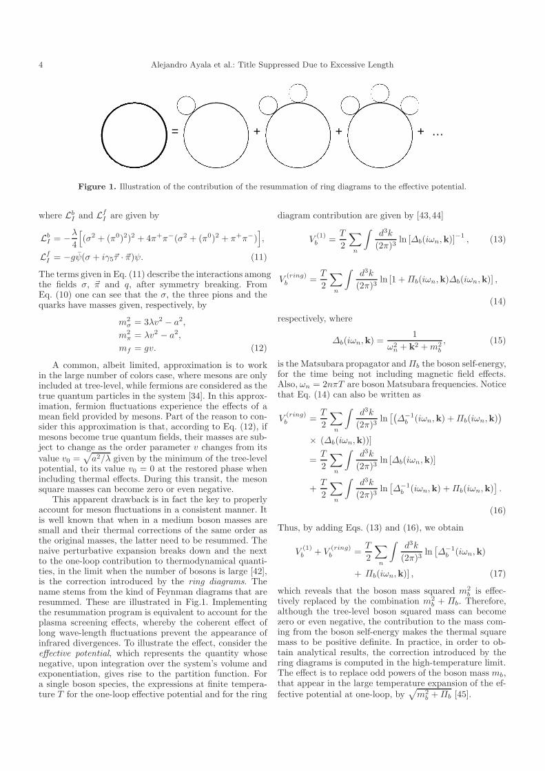
= + + ...+
Figure 1. Illustration of the contribution of the resummation of ring diagrams to the effective potential.
where LbI and LfI are given by
LbI = −λ4
[
(σ2 + (π0)2)2 + 4π+π−(σ2 + (π0)2 + π+π−)]
,
LfI = −gψ(σ + iγ5~τ · ~π)ψ. (11)
The terms given in Eq. (11) describe the interactions amongthe fields σ, ~π and q, after symmetry breaking. FromEq. (10) one can see that the σ, the three pions and thequarks have masses given, respectively, by
m2σ = 3λv2 − a2,
m2π = λv2 − a2,
mf = gv. (12)
A common, albeit limited, approximation is to workin the large number of colors case, where mesons are onlyincluded at tree-level, while fermions are considered as thetrue quantum particles in the system [34]. In this approx-imation, fermion fluctuations experience the effects of amean field provided by mesons. Part of the reason to con-sider this approximation is that, according to Eq. (12), ifmesons become true quantum fields, their masses are sub-ject to change as the order parameter v changes from itsvalue v0 =
√
a2/λ given by the minimum of the tree-levelpotential, to its value v0 = 0 at the restored phase whenincluding thermal effects. During this transit, the mesonsquare masses can become zero or even negative.
This apparent drawback is in fact the key to properlyaccount for meson fluctuations in a consistent manner. Itis well known that when in a medium boson masses aresmall and their thermal corrections of the same order asthe original masses, the latter need to be resummed. Thenaive perturbative expansion breaks down and the nextto the one-loop contribution to thermodynamical quanti-ties, in the limit when the number of bosons is large [42],is the correction introduced by the ring diagrams. Thename stems from the kind of Feynman diagrams that areresummed. These are illustrated in Fig.1. Implementingthe resummation program is equivalent to account for theplasma screening effects, whereby the coherent effect oflong wave-length fluctuations prevent the appearance ofinfrared divergences. To illustrate the effect, consider theeffective potential, which represents the quantity whosenegative, upon integration over the system’s volume andexponentiation, gives rise to the partition function. Fora single boson species, the expressions at finite tempera-ture T for the one-loop effective potential and for the ring
diagram contribution are given by [43,44]
V(1)b =
T
2
∑
n
∫
d3k
(2π)3ln [∆b(iωn,k)]
−1, (13)
V(ring)b =
T
2
∑
n
∫
d3k
(2π)3ln [1 +Πb(iωn,k)∆b(iωn,k)] ,
(14)
respectively, where
∆b(iωn,k) =1
ω2n + k2 +m2
b
, (15)
is the Matsubara propagator andΠb the boson self-energy,for the time being not including magnetic field effects.Also, ωn = 2nπT are boson Matsubara frequencies. Noticethat Eq. (14) can also be written as
V(ring)b =
T
2
∑
n
∫
d3k
(2π)3ln[(
∆−1b (iωn,k) +Πb(iωn,k)
)
× (∆b(iωn,k))]
=T
2
∑
n
∫
d3k
(2π)3ln [∆b(iωn,k)]
+T
2
∑
n
∫
d3k
(2π)3ln[
∆−1b (iωn,k) +Πb(iωn,k)
]
.
(16)
Thus, by adding Eqs. (13) and (16), we obtain
V(1)b + V
(ring)b =
T
2
∑
n
∫
d3k
(2π)3ln[
∆−1b (iωn,k)
+ Πb(iωn,k)] , (17)
which reveals that the boson mass squared m2b is effec-
tively replaced by the combination m2b + Πb. Therefore,
although the tree-level boson squared mass can becomezero or even negative, the contribution to the mass com-ing from the boson self-energy makes the thermal squaremass to be positive definite. In practice, in order to ob-tain analytical results, the correction introduced by thering diagrams is computed in the high-temperature limit.The effect is to replace odd powers of the boson mass mb,that appear in the large temperature expansion of the ef-fective potential at one-loop, by
√
m2b +Πb [45].

Alejandro Ayala et al.: Title Suppressed Due to Excessive Length 5
2.1 One-loop boson contribution
We now turn to finding the boson contribution to the effec-tive potential for the LSMq in the presence of a magneticfield [46]. The Matsubara propagator for a boson with elec-tric charge qb can now be written in terms of Schwinger’sproper time representation as
∆b(iωn,k; |qbB|) =∫ ∞
0
ds
cosh |qbB|s
× exp
−s(
ω2n + k23 + k2⊥
tanh |qbB|s|qbB|s +m2
b
)
.
(18)
Therefore, the one-loop contribution to the effective po-tential Eq. (13) becomes in the presence of the magneticfield
V(1;B)b =
T
2
∑
n
∫
d3k
(2π)3ln [∆b(iωn,k; |qbB|)]−1
. (19)
Using that
ln [∆b(iωn,k; |qbB|)]−1
=
∫
dm2b
(
d
dm2b
ln [∆b(iωn,k; |qbB|)]−1
)
=
∫
dm2b ∆b(iωn,k; |qbB|), (20)
we obtain
V(1;B)b =
T
2
∑
n
∫
dm2b
∫
d3k
(2π)3
∫ ∞
0
ds
cosh |qbB|s
× exp
−s(
ω2n + k23 + k2⊥
tanh |qbB|s|qbB|s +m2
b
)
.
(21)
Performing the integration over k⊥, introducing the sumover Landau levels, integrating over s, performing the sumover Matsubara frequencies and the integration over m2
b ,in that order, we get
V(1;B)b =
|qbB|4π
∑
l
∫ ∞
−∞
dk32π
[
ωl + 2T ln(
1− e−ωl/T)]
,
(22)
where
ωl =√
k23 +m2b + (2l+ 1)|qbB|. (23)
Notice that Eq. (22) splits into vacuum and matter con-tributions, namely
V(1;B vac)b =
|qbB|4π
∑
l
∫ ∞
−∞
dk32π
ωl, (24)
and
V(1;B matt)b =
2|qbB|4π
T∑
l
∫ ∞
−∞
dk32π
ln(
1− e−ωl/T)
.
(25)
We now specialize to implementing the calculation hav-ing in mind the conditions after a relativistic heavy-ioncollision. Recall that in this environment, although themagnetic field intensity can be initially very large, it de-creases fast such that, for the time the plasma reachesthermal equilibrium, it becomes weak. Under such condi-tions, it seems plausible to compute the effective poten-tial, in the weak field limit. For this purpose let us writeEq. (22) as
V(1;B vac)b =
Sb2, (26)
where
Sb ≡∑
l
h
4πfl
fl ≡∫ ∞
−∞
dk32π
ωl, (27)
with h = 2|qbB|. The sum can be performed resorting tothe Euler-Mclaurin formula, writing
h
[
f02
+ f1 + f2 + . . .+fN2
]
=
∫ Nh
0
dxf(x)
+B2
2!h2(f ′
N − f ′0), (28)
where B2 = 1/6 is the second Bernoulli number and wehave kept terms only up to O(qbB)2. The limit N → ∞is to be understood. Notice that on the right-hand side ofEq. (28) we made the replacement 2|qbB|(l + 1/2) → x,which means that, if we think of the series of fl as beingrepresented by a histogram, we are effectively performingthe sum evaluating the function at the middle point ofeach bar in the histogram. This means that on the left-hand side of Eq. (28), the first and last terms in the sumare weighed with h/2. For small |qbB|, x can be thoughtof as being continuous, and the derivative is taken withrespect to this variable. The meaning of x can in turn bemade more appealing by writing
x = k2⊥,
dx = dk2⊥ = 2k⊥dk⊥, (29)
therefore∫ Nh
0
dxf(x) → 2(2π)
∫
d3k
(2π)3
√
k2 +m2b , (30)
and
f ′ ≡ df
dk2⊥=
1
2
∫ ∞
−∞
dk32π
1√
k2 +m2b
(f ′∞ − f ′
0) = −1
2
∫ ∞
−∞
dk32π
1√
k23 +m2b
. (31)
Hence, bringing all together we get
V(1;B vac)b =
1
2
∫
d3k
(2π)3
√
k2 +m2b
− |qbB|248π
∫ ∞
−∞
dk32π
1√
k23 +m2b
. (32)
6 Alejandro Ayala et al.: Title Suppressed Due to Excessive Length
In order to find an explicit expression, we use dimensionalregularization, introducing the ultraviolet renormalizationscale µ in the MS scheme, to get
V(1;B vac)b =
m4b
64π2
[
ln
(
m2b
µ2
)
− 1
ǫ− 3
2
]
+|qbB|296π2
[
ln
(
m2b
µ2
)
− 1
ǫ
]
. (33)
Notice that the divergent piece in the first line of Eq. (33)is harmless as it is T and B-independent and can be safelyignored. On the other hand, the divergent term in thesecond line of Eq. (33) is potentially dangerous since itis B-dependent. However, recall that the vacuum massdivergence is cured precisely by the inclusion of a masscounterterm δm2 ∼ m2/ǫ. Therefore, the addition of thiscounterterm in the second line of Eq. (33) effectively in-duces the substitution
ln
[
m2b
µ2
]
→ ln
[
m2b
µ2
(
1 +1
ǫ
)]
∼ ln
[
m2b
µ2
]
+1
ǫ. (34)
Therefore, the renormalized vacuum contribution is writ-ten as
V(1;B ren)b =
m4b
64π2
[
ln
(
m2b
µ2
)
− 3
2
]
+|qbB|296π2
[
ln
(
m2b
µ2
)]
. (35)
We now look at the matter contribution to the one-loop effective potential, Eq. (25), which we write as
V(1;B matt)b = TSmattb , (36)
where
Smattb =∑
l
h
4πgl,
gl ≡∫ ∞
−∞
dk32π
ln(
1− e−ωl/T)
. (37)
Once again, working in the weak field limit we can write
h[g02
+ g1 + g2 + . . .+gN2
]
=
∫ Nh
0
dxg(x)
+B2
2!h2(g′N − g′0). (38)
In the limit N → ∞∫ Nh
0
dx g(x) → 2(2π)
∫
d3k
(2π)3ln(
1− e−√k2+m2
b/T)
,
(39)and
g′ ≡ dg
dk2⊥=
1
2T
∫ ∞
−∞
dk32π
1√
k2 +m2b
(
1
e√k2+m2
b/T − 1
)
,
(g′∞ − g′0) = − 1
2T
∫ ∞
−∞
dk32π
1√
k23 +m2b
(
1
e√k23+m2
b/T − 1
)
.
(40)
Thus
V(1;B matt)b = T
∫
d3k
(2π)3ln(
1− e−√k2+m2
b/T)
− |qbB|224π
∫ ∞
−∞
dk32π
1√
k23 +m2b
×(
1
e√k23+m2
b/T − 1
)
. (41)
We now proceed to provide an approximate expressionfor Eq. (41) in the large T -limit. The first term is givenby [42]
T
∫
d3k
(2π)3ln(
1− e−√k2+m2
b/T)
≃ −T4π2
90+T 2m2
b
24− Tm3
b
12π− m4
b
64π2
[
ln
(
m2b
(4πT )2
)
+ 2γE − 3
2
]
. (42)
For the second term we get [44]
−|qbB|224π
∫ ∞
−∞
dk32π
1√
k23 +m2b
(
1
e√k23+m2
b/T − 1
)
≃ −|qbB|224π2
[
Tπ
2mb+
1
4ln
(
m2b
(4πT )2
)
+1
2γE
− 1
4ζ(3)
(
m2b
(2πT )2
)
+3
16ζ(5)
(
m4b
(2πT )4
)]
,
(43)
Alejandro Ayala et al.: Title Suppressed Due to Excessive Length 7
where γE and ζ are the Euler-Mascheroni constant andRiemann Zeta function, respectively. Notice that the ar-guments of the logarithms in Eqs. (35), (42) and (35) arepotentially dangerous when m2
b becomes zero or even neg-ative. However, when adding up these equations to express
the one-loop boson contribution to the effective potential,these terms combine in such a way that the argument ofthe logarithms does not contain m2
b anymore. We thus ob-tain
V(1;B ren)b + V
(1;B matt)b = −T
4π2
90+T 2m2
b
24− Tm3
b
12π− m4
b
64π2
[
ln
(
µ2
(4πT )2
)
+ 2γE
]
− |qbB|224π2
[
Tπ
2mb+
1
4ln
(
µ2
(4πT )2
)
+1
2γE − 1
4ζ(3)
(
m2b
(2πT )2
)
+3
16ζ(5)
(
m4b
(2πT )4
)]
. (44)
Notice however that Eq. (44) contains odd powers of
mb =√
m2b . When the boson mass squared is negative,
these terms become imaginary. This instability is non-physical and, as we proceed to show, it can be cured byconsidering the contribution from the ring diagrams.
2.2 Ring contribution
Recall that from Eq. (16), the ring contribution to theeffective potential can be written as
V(ring)b =
T
2
∑
n
∫
d3k
(2π)3(
ln[
∆−1b (iωn,k) +Πb(iωn,k)
]
− ln[
∆−1b (iωn,k)
])
. (45)
At high temperature, the leading ring contribution comesfrom the n = 0 Matsubara mode, so we write
V(ring)b =
T
2
∫
d3k
(2π)3(
ln[
∆−1b (iω0,k) +Πb
]
− ln[
∆−1b (iω0,k)
])
, (46)
where we have also approximated Πb by a momentum in-dependent quantity. This choice will be justified later onwhen we discuss the computation of the self-energy. Equa-tion (46) contains two terms. The first one is obtained fromthe second by the replacement m2
b → m2b +Πb. Therefore
we concentrate on the computation of the second term
T
2
∫
d3k
(2π)3ln[
∆−1b (iω0,k)
]
=T
2
∫
dm2b
∫
d3k
(2π)3d
dm2b
ln[
∆−1b (iω0,k)
]
=T
2
∫
dm2b
∫
d3k
(2π)3∆b(iω0,k)
=T
2
∫
dm2b
∫
d3k
(2π)3
∫ ∞
0
ds
cosh |qbB|se−s
(
k23+k2⊥
tanh |qbB|s
|qbB|s +m2b
)
.
(47)
Performing the integration over k⊥ we obtain
T
2
∫
d3k
(2π)3ln[
∆−1b (iω0,k)
]
= T
( |qbB|8π
)∫
dm2b
∫ ∞
−∞
dk32π
∫ ∞
0
ds
sinh |qbB|se−s(k23+m2
b).
(48)
Introducing the series representation
1
sinh(x)= 2
∞∑
l=0
e−(2l+1)x, (49)
we get
T
2
∫
d3k
(2π)3ln[
∆−1b (iω0,k)
]
= T
( |qbB|4π
)∫
dm2b
∫ ∞
−∞
dk32π
∞∑
l=0
∫ ∞
0
ds e−s(k23+m
2b+(2l+1)|qbB|). (50)
8 Alejandro Ayala et al.: Title Suppressed Due to Excessive Length
Carrying out the integrations over s and k3, we have
T
2
∫
d3k
(2π)3ln[
∆−1b (iω0,k)
]
= T
( |qbB|8π
) ∞∑
l=0
∫
dm2b
√
m2b + (2l + 1)|qbB|
= T
(
2|qbB|8π
) ∞∑
l=0
√
m2b + (2l+ 1)|qbB|.
(51)
For the weak field case, we can once again use the Euler-Maclaurin formula to write
T
2
∫
d3k
(2π)3ln[
∆−1b (iω0,k)
]
=
(
T
8π
)
∫ Λ2
0
dx√
m2b + x− |qbB|2
6mb
=
(
T
8π
)
2
3
(
m2b + Λ2
)3/2 − 2
3m2b −
|qbB|26mb
≃(
T
12π
)
Λ3 −m3b −
|qbB|24mb
, (52)
where, since the integral on the right-hand side diverges,the upper limit of integration has been set as the largebut finite quantity Λ2. The dependence of the result onΛ will drop out wen including the Πb-dependent term inEq. (45). Using a similar procedure to treat the first termof Eq. (46), we obtain
V(ring)b =
(
T
12π
)
m3b − (m2
b +Πb)3/2
+|qbB|24mb
− |qbB|24(m2
b +Πb)1/2
, (53)
where, as promised, the dependence on Λ has dropped out.Therefore, adding this contribution to Eq. (44), we get
V(eff)b ≡ V
(1;B ren)b + V
(1;B matt)b + V
(ring)b =
− T 4π2
90+T 2m2
b
24− T (m2
b +Πb)3/2
12π
− m4b
64π2
[
ln
(
µ2
(4πT )2
)
+ 2γE
]
− |qbB|224π2
[
Tπ
2(m2b +Πb)1/2
+1
4ln
(
µ2
(4πT )2
)
+1
2γE − 1
4ζ(3)
(
m2b
(2πT )2
)
+3
16ζ(5)
(
m4b
(2πT )4
)]
.
(54)
We thus confirm that the inclusion of the ring diagramsproduces an effective potential which is free of infraredinstabilities. In order to use this expression to study thephase diagram, it is necessary to compute the boson self-energy Πb. Before we proceed to this calculation, we firstcompute the contribution from fermions to the effectivepotential.
2.3 One-loop fermion contribution
We start from the expression for the one-loop effective po-tential for one fermion species. Working first in Minkowsky
space, this expression is given by
V(1;B)f = i lnDet(iS−1
f )
= iTr ln(iS−1f )
= iTr ln( /Π −mf ), (55)
where Sf is the fermion propagator in the presence of amagnetic field, Πµ = pµ − qfAµ is the kinematical mo-mentum and qf , mf are the fermion electric charge andmass, respectively. In order to find a working expression,notice that
Det( /Π +mf )Det( /Π −mf ) = Det[
( /Π +mf )( /Π −mf )]
= Det[
/Π2 −m2
f
]
, (56)
then
lnDet[
/Π2 −m2
f
]
= lnDet( /Π +mf ) + lnDet( /Π −mf).
(57)
Also, since in four space-time dimensions
Det( /Π +mf ) = Det[
γ25( /Π +mf )]
= Det[
γ5(− /Π +mf )γ5]
= Det( /Π −mf ), (58)
we have
lnDet( /Π +mf) + lnDet( /Π −mf ) = 2 lnDet( /Π −mf ).
(59)
Therefore, using Eq. (57), we have
lnDet( /Π −mf ) =1
2lnDet( /Π
2 −m2f ), (60)
and all in all, we get
V(1;B)f =
i
2Tr ln( /Π
2 −m2f ). (61)
Recall that
/Π2= Π2 − qfBΣ3, (62)

Alejandro Ayala et al.: Title Suppressed Due to Excessive Length 9
whereΣ3 is the spin operator along the z-axis. We thus seethat after accounting for the trace, the expression for thefermion contribution to the one-loop effective potential isequivalent to minus the contribution from four scalars, twoof them carrying a label representing the spin projectionparallel and the other two antiparallel to the magneticfield. The spin projection can be more easily implementedintroducing a sum over an index σ that takes on the values±1. Since both components are involved, it is enough towrite qfBΣ3 → |qfB|σ. Therefore, the expression for thefermion contribution to the one-loop effective potential atfinite temperature is written as
V(1;B)f =−2
∑
σ=±1
T
2
∑
n
∫
dm2f
∫
d3k
(2π)3
∫ ∞
0
ds
cosh |qbB|s
× e−s
[
(ωn+iµ)2+k23+k
2⊥
tanh |qbB|s
|qbB|s +m2f+σ|qfB|
]
,
(63)
where ωn = (2n+1)πT is a fermion Matsubara frequencyand µ is the quark chemical potential. The factor of 2 andthe sum over σ take care of the four fermion degrees offreedom.
Performing the integration over k⊥, introducing thesum over Landau levels, integrating over s, performingthe sum over Matsubara frequencies and the integrationover m2
f , in that order, we get
V(1;B)f = −2|qfB|
4π
∑
l,σ
∫ ∞
−∞
dk32π
[ωl
+ T ln(
1 + e−(ωl−µ)/T)
+ T ln(
1 + e−(ωl+µ)/T)]
, (64)
where
ωl =√
k23 +m2f + (2l+ 1 + σ)|qfB|. (65)
Once again in Eq. (65) we distinguish two kinds ofterms, vacuum and matter contributions, namely
V(1;B vac)f = −2|qfB|
4π
∑
l,σ
∫ ∞
−∞
dk32π
ωl, (66)
and
V(1;B matt)f = −2|qfB|
4πT∑
l,σ
∫ ∞
−∞
dk32π
×[
ln(
1 + e−(ωl−µ)/T)
+ ln(
1 + e−(ωl+µ)/T)]
. (67)
We now proceed to compute each of these contribu-tions separately. We start with the vacuum contribution.
Writing the sum over σ explicitly, we get
V(1;B vac)f =−2|qfB|
4π
∞∑
l=0
∫ ∞
−∞
dk32π
×[√
k23 +m2f + 2(l + 1)|qfB|
+√
k23 +m2f + 2l|qfB|
]
. (68)
We now separate the term with l = 0 writing
V(1;B vac)f = −2|qfB|
4π
∫ ∞
−∞
dk32π
[√
k23 +m2f
+ 2
∞∑
l=1
√
k23 +m2f + 2l|qfB|
]
. (69)
Let us first compute the term with the sum. Define
Sf ≡∞∑
l=1
h
4πfl
fl ≡ 2
∫ ∞
−∞
dk32π
√
k23 +m2f + 2l|qfB|, (70)
where h = 2|qfB|. Notice that, were we to represent theseries of fl by a histogram, the function would then beevaluated at the edges of each bar. Thus, the expressionfor the Euler-Maclaurin formula to use is
h
[
f1 + f2 + . . .+fN2
]
=
∫ Nh
0
dxf(x)− hf(0)
2
+B2
2!h2(f ′
N − f ′0), (71)
where again, B2 = 1/6 and we have kept terms only up toO(qfB)2. Notice that we have maintained the last termon the left-hand side as fN/2 since in the limit when N →∞ this does not make a difference and the divergence isanyway taken care of by using dimensional regularizationfor the expression on the right-hand side. Also, in Eq. (71),the contribution from the term −f(0)/2 cancels the firstterm on the right-hand side of Eq. (69).
We now make the change of variable in Eq. (29) towrite
∫ Nh
0
dxf(x) → 2(4π)
∫
d3k
(2π)3
√
k2 +m2f (72)
and
f ′ ≡ df
dk2⊥=
∫ ∞
−∞
dk32π
1√
k2 +m2f
(f ′∞ − f ′
0) = −∫ ∞
−∞
dk32π
1√
k23 +m2f
. (73)
Writing these ingredients all together, we have
V(1;B vac)f = −2
∫
d3k
(2π)3
√
k2 +m2f
− |qfB|212π
∫ ∞
−∞
dk32π
1√
k23 +m2f
. (74)
10 Alejandro Ayala et al.: Title Suppressed Due to Excessive Length
Therefore, working in the MS scheme and after accountingfor the fermion mass renormalization, we get
V(1;B ren)f =
m4f
16π2
[
ln
(
µ2
m2f
)
+3
2
]
+|qfB|224π2
[
ln
(
µ2
m2f
)]
. (75)
We now turn to the calculation of the matter contri-bution, Eq. (67), which, after accounting for the sum overσ and separating the term of the sum with l = 0 can bewritten as
V(1;B matt)f = −2|qfB|
4πT
∫ ∞
−∞
dk32π
×[
ln(
1 + e−(√k23+m2
f−µ)/T
)
+ ln(
1 + e−(√k23+m2
f+µ)/T
)]
+
∞∑
l=1
[
ln(
1 + e−(√k23+m2
f+2l|qfB|−µ)/T
)
+ ln(
1 + e−(√k23+m2
f+2l|qfB|+µ)/T
)]
.
(76)
In order to employ the Euler-Maclaurin formula up toO(qfB)2, we write
h [g1 + . . .+ gN ] =
∫ Nh
0
dxg(x) + hg(Nh)− g(0)
2
+B2
2!h2(g′N − g′0), (77)
and identify
gl = 2
∫ ∞
−∞
dk32π
[
ln(
1 + e−(√k23+m2
f+2l|qfB|−µ)/T
)
+ ln(
1 + e−(√k23+m2
f+2l|qfB|+µ)/T
)]
, (78)
with h = 2|qfB|. Notice that
g∞ = 0
g0 = 2
∫ ∞
−∞
dk32π
[
ln(
1 + e−(√k23+m2
f−µ)/T
)
+ ln(
1 + e−(√k23+m2
f+µ)/T
)]
, (79)and we obtain
V(1;B matt)f = −2 T
∫
d3k
(2π)3
[
ln(
1 + e−(√k2+m2
f−µ)/T
)
+ ln(
1 + e−(√k2+m2
f+µ)/T
)]
− |qfB|212π
∫ ∞
−∞
dk32π
1√
k23 +m2f
×[
1
e(√k23+m2
f−µ)/T + 1
+1
e(√k23+m2
f+µ)/T + 1
]
.
(80)
We now look for a large-T approximation for Eq. (80). Letus start working the second term. We write
x =k3T
y =mf
T
z =µ
T, (81)
and use that
1√
x2 + y2
1
e√x2+y2−z
+1
e√x2+y2+z
=1
√
x2 + y2− 2
∞∑
n=−∞
1
[(2n+ 1)π + iz]2 + x2 + y2
=1
√
x2 + y2− 2
∞∑
n=−∞
1(
[(2n+ 1)π + iz]2+ y2
)(
1 + x2
[(2n+1)π+iz]2+y2
) .
(82)
Thus, the integral in the second term of Eq. (80) can be expressed in terms of two terms given by
I1 =
∫ ∞
0
xǫdx√
x2 + y2
I2 = −2∞∑
n=−∞
∫ ∞
0
xǫdx(
[(2n+ 1)π + iz]2+ y2
)(
1 + x2
[(2n+1)π+iz]2+y2
) , (83)

Alejandro Ayala et al.: Title Suppressed Due to Excessive Length 11
with∫ ∞
−∞
dk32π
1√
k23 +m2f
[
1
e(√k23+m2
f−µ)/T
+1
e(√k23+m2
f+µ)/T
]
=1
π(I1 + I2). (84)
Notice that, in anticipation to treating the divergenceof each term, we have introduced the regulating factorxǫ. As we proceed to show, this divergence cancels whenadding both terms. First, notice that
I1 =y−ǫ
2√πΓ
[
1
2− ǫ
2
]
=1
ǫ− γE
2− 1
2ψ0
(
1
2
)
− ln (y). (85)
For the computation of I2, we define
ω2n = [(2n+ 1)π + iz]
2, (86)
and introduce the change of variable
u =x
√
ω2n + y2
, (87)
to write
I2 = −2
∞∑
n=−∞
1
(ω2 + y2)1+ǫ2
∫ ∞
0
duuǫ
(1 + u2). (88)
The integral can be expressed as
∫ ∞
0
duuǫ
(1 + u2)=π
2sec(πǫ
2
)
=π
2, (89)
where we used that for ǫ→ 0, the series of sec(ǫ) starts atO(ǫ)2 and thus its ǫ dependence can be discarded. There-fore
I2 = −π∞∑
n=−∞
1
(ω2n + y2)
1+ǫ2
= −π∑
s=±1
∞∑
n=0
1(
[(2n+ 1)π + isz]2+ y2
)1+ǫ2
. (90)
To look for an expression to O(y2), we expand the denom-inator of Eq. (90) to obtain
1(
[(2n+ 1)π + isz]2 + y2)
1+ǫ2
=1
[(2n+ 1)π + isz]1+ǫ2
− (1 + ǫ)
2
y2
[(2n+ 1)π + isz]3+ǫ ,
(91)
therefore
I2 = −π∑
s=±1
1
(2π)1+ǫζ
(
1 + ǫ,1
2+isz
2π
)
− (1 + ǫ)
2
y2
(2π)3+ǫζ
(
3 + ǫ,1
2+isz
2π
)
, (92)
where ζ is the Hurwitz Zeta function. Expanding for smallǫ we get
I2 = −1
ǫ+ 2 ln(2π)− ψ0
(
1
2+iz
2π
)
− ψ0
(
1
2− iz
2π
)
+y2
16π2
[
ζ
(
3,1
2+iz
2π
)
+ ζ
(
3,1
2− iz
2π
)]
, (93)
where ψ0 is the digamma function. Adding up Eqs. (85)and (93) we obtain
− |qfB|212π
∫ ∞
−∞
dk32π
1√
k23 +m2f
×[
1
e(√k23+m2
f−µ)/T
+1
e(√k23+m2
f+µ)/T
]
= −|qfB|212π2
2 ln(2π)− γE − 1
2ψ0
(
1
2
)
− 1
2ψ0
(
1
2+
iµ
2πT
)
− 1
2ψ0
(
1
2− iµ
2πT
)
+1
2ln
(
4π2T 2
m2f
)
+m2f
16π2T 2
[
ζ
(
3,1
2+
iµ
2πT
)
+ ζ
(
3,1
2− iµ
2πT
)]
. (94)
12 Alejandro Ayala et al.: Title Suppressed Due to Excessive Length
To evaluate the first term in Eq. (80) in the large-T limit,we carry out a similar procedure. We first notice that inorder to obtain an expansion of the integral up to O(m4
f ),we can take the second derivative of
J(mf/T ) ≡ −2T
∫
d3k
(2π)3
[
ln(
1 + e−(√k2+m2
f−µ)/T
)
+ ln(
1 + e−(√k2+m2
f+µ)/T
)]
, (95)
with respect to m2f and look for an approximation for
d2J/(dm2f )
2 up to the desired order. This approach ren-
ders analytical results provided J(0) and dJ/dm2f (0) can
be computed analytically. In such case, their values canbe used as the boundary conditions to find the solution.It is straightforward to show that indeed this is the caseand that
J(0) =T 4
π2
[
Li4
(
−e− µT
)
+ Li4
(
−e µT
)]
,
dJ
dm2f
(0) = − T 2
2π2
[
Li2
(
−e− µT
)
+ Li2
(
−e µT
)]
, (96)
where Lin is the polylogarithmic function of order n. Theapproximation of d2J/(dm2
f )2 up to O(m2
f ) is found using
the same procedure employed to find Eq. (94) and the
result is
d2J
(dm2f )
2=
1
8π2
[
ln
(
m2f
T 2
)
+ ψ0
(
3
2
)
− ψ0
(
1
2+
iµ
2πT
)
− ψ0
(
1
2− iµ
2πT
)
− 2 (1 + ln(2π)) + γE
]
. (97)
We now integrate Eq. (97) considering it as a differen-tial equation and implementing Eqs. (96) as the boundaryconditions for the first derivative and the function itself.Integrating Eq. (97) once, we obtain
J(m2f ) =
m4f
16π2
[
ln
(
m2f
T 2
)
− 3
2+ ψ0
(
3
2
)
− ψ0
(
1
2+
iµ
2πT
)
− ψ0
(
1
2− iµ
2πT
)
− 2 (1 + ln(2π)) + γE
]
+ C1m2f + C2. (98)
Using the set of Eqs. (97), we infer that
C1 = − T 2
2π2
[
Li2
(
−e− µT
)
+ Li2
(
−e µT
)]
,
C2 =T 4
π2
[
Li4
(
−e− µT
)
+ Li4
(
−e µT
)]
. (99)
Therefore, writing Eqs. (75), (94), and (98) together, thecontribution from one fermion species to the one-loop ef-fective potential is
V(1;B ren)f + V
(1;B matt)f =
m4f
16π2
[
ln
(
µ2
m2f
)
+3
2
]
+|qfB|224π2
[
ln
(
µ2
m2f
)
]
+m4f
16π2
[
ln
(
m2f
T 2
)
− 3
2+ ψ0
(
3
2
)
− ψ0
(
1
2+
iµ
2πT
)
− ψ0
(
1
2− iµ
2πT
)
− 2(1 + ln (2π)) + γE
]
−m2fT
2
2π2
[
Li2(−e−µT ) + Li2(−e
µT )]
− |qfB|212π2
2 ln (2π)− γE − 1
2ψ0
(
1
2
)
− 1
2ψ0
(
1
2+
iµ
2πT
)
− 1
2ψ0
(
1
2− iµ
2πT
)
+1
2ln
(
4π2T 2
m2f
)
+m2f
16π2T 2
[
ζ
(
3,1
2+
iµ
2πT
)
+ ζ
(
3,1
2− iµ
2πT
)]
. (100)
Equation (100) possesses the remarkable property that potentially offending logarithmic terms, as the fermion massvanishes, combine to trade the mass dependence by a temperature dependence. Thus, bringing together these terms

Alejandro Ayala et al.: Title Suppressed Due to Excessive Length 13
and simplifying, we obtain
V(eff)f ≡ V
(1;B ren)f + V
(1;B matt)f =
m4f
16π2
[
ln
(
µ2
T 2
)]
+|qfB|224π2
[
ln
(
µ2
4π2T 2
)]
+m4f
16π2
[
ψ0
(
3
2
)
− 2 (1 + ln(2π)) + γE
− ψ0
(
1
2+
iµ
2πT
)
− ψ0
(
1
2− iµ
2πT
)
]
−m2fT
2
2π2
[
Li2
(
−e− µT
)
+ Li2
(
−e µT
)]
+T 4
π2
[
Li4
(
−e− µT
)
+ Li4
(
−e µT
)]
− |qfB|212π2
2 ln(2π)− γE − 1
2ψ0
(
1
2
)
− 1
2ψ0
(
1
2+
iµ
2πT
)
− 1
2ψ0
(
1
2− iµ
2πT
)
+m2f
16π2T 2
[
ζ
(
3,1
2+
iµ
2πT
)
+ ζ
(
3,1
2− iµ
2πT
)]
.
(101)
Before writing together the fermion and boson contri-butions to the effective potential, it is necessary to dis-cuss the conditions that need to be implemented to avoidthat the inclusion of the one-loop corrections distort thevacuum of the theory from where the particle masses aredefined. These are the vacuum stability conditions.
2.4 Vacuum stability
In order to complete the description of the effective poten-tial, it is important to notice that the vacuum, one-loopB-independent corrections, distort the original tree-levelpotential. This distortion manifest itself in a shift of theminimum and its curvature in the σ-direction. When ig-nored, this distortion leads to changes in what we iden-tify as the vacuum σ, pion and fermion masses. Howeverit is clear that our description of the vacuum at any or-der in perturbation theory should be consistent with themeasured vacuum particle masses. This means that thevacuum distortion needs to be compensated in such a waythat its properties, directly related to particle masses, keepbeing the same as if these properties were defined fromthe tree-level potential. This procedure is dubbed vacuumstabilization [47]. When vacuum stability is not consid-ered, the description of the nature of the phase transitioncan lead to drastically different results such as the possi-ble splitting of the deconfinement and chiral transitions inan external magnetic field. This scenario has been stud-ied in Ref. [48] within the LSMq coupled to a Polyakovloop. The authors found that the vacuum correction fromquarks on the phase structure was dramatic. When ignor-ing this correction, the confinement and chiral phase tran-sition lines coincide. However, inclusion of the correction
led to a splitting of the confinement and chiral transitionlines, and both chiral and deconfining critical tempera-tures became increasing functions of the magnetic field.The vacuum contribution from the quarks drastically af-fected the chiral sector as well. Since these conclusionswere drawn from a model that does not reproduce thebehavior of the critical temperature as a function of themagnetic field found by lattice QCD calculations, theyare nowadays regarded as incorrect. Furthermore, LQCDresults shows that no significant difference between chi-ral and deconfinement transition temperatures exists upto fields as intense as 3.25 GeV2 [30]. In order to stabilizethe vacuum at one-loop level, we look at the tree-level plusone-loop B-independent fermion and boson vacua. For thelatter we only include the potential in the direction of the
V(tree)
V(vac)
0 50 100 150 200
-0.30
-0.25
-0.20
-0.15
-0.10
-0.05
0.00
v [MeV]
V(eff) /a4
Figure 2. Comparison between the tree-level and stabilizedvacua. Notice that inclusion of the vacuum stability conditionsproduces that both terms coincide around the minimum.
14 Alejandro Ayala et al.: Title Suppressed Due to Excessive Length
σ-field. These contributions are given by
V (vac) ≡ V (tree) + V (1)σ + V
(1)f
= −a2
2v2 +
λ
4v4 − δa2
2v2 +
δλ
4v4
+m4σ
64π2
[
ln
(
m2σ
µ2
)
− 3
2
]
− NcNfm4f
16π2
[
ln
(
m2f
µ2
)
− 3
2
]
, (102)
where we have accounted for the contribution ofNcNf = 6fermions, corresponding to Nc colors and Nf flavors andhave introduced the counterterms δa2 and δλ. These coun-terterms need to be fixed from the conditions to keep thevacuum and its curvature at their tree-value levels, namely
1
v
dV (vac)
dv
∣
∣
∣
v=v0= 0,
d2V (vac)
dv2
∣
∣
∣
v=v0= 2a2, (103)
where v0 =√
a2/λ is the value of v at the tree-level min-imum. The solution for the counterterms δa2 and δλ aregiven by
δa2 = − 3a2
16π2
[
λ ln
(
2a2
µ2
)
− 8g4
λ+ 2λ
]
,
δλ =3
16π2
[
8g4 ln
(
g2a2
λµ2
)
− 3λ2 ln
(
2a2
µ2
)]
. (104)
Figure 2 shows the three level potential V (tree) comparedto the vacuum potential V (vac) after implementing thestabilization procedure. Notice that both coincide near theminimum.
Writing all the ingredients together, the effective po-tential up to the ring diagrams contribution and after vac-uum stabilization can be written as
V (eff) = −a2
2
1 +3a2
8π2
[
λ ln
(
2a2
µ2
)
− 8g4
λ+ 2λ
]
v2
+λ
4
1 +3
4π2
[
8g4 ln
(
g2a2
λµ2
)
− 3λ2 ln
(
2a2
µ2
)]
v4
+∑
b=π±,π0,σ
−T4π2
90+T 2m2
b
24− T (m2
b +Πb)3/2
12π− m4
b
64π2
[
ln
(
µ2
(4πT )2
)
+ 2γE
]
− |qbB|224π2
∑
b=π±
Tπ
2(m2b +Πb)1/2
+1
4ln
(
µ2
(4πT )2
)
+1
2γE
− 1
4ζ(3)
(
m2b
(2πT )2
)
+3
16ζ(5)
(
m4b
(2πT )4
)
+ NcNf
m4f
16π2
[
ln
(
µ2
T 2
)
− ψ0
(
1
2+
iµ
2πT
)
− ψ0
(
1
2− iµ
2πT
)
+ ψ0
(
3
2
)
− 2 (1 + ln(2π)) + γE
]
−m2fT
2
2π2
[
Li2
(
−e− µT
)
+ Li2
(
−e µT
)]
+T 4
π2
[
Li4
(
−e− µT
)
+ Li4
(
−e µT
)]
+|qfB|212π2
(
1
2ln
(
µ2
4π2T 2
)
+1
2ψ0
(
1
2+
iµ
2πT
)
+1
2ψ0
(
1
2− iµ
2πT
)
+1
2ψ0
(
1
2
)
− 2 ln(2π) + γE −m2f
16π2T 2
[
ζ
(
3,1
2+
iµ
2πT
)
+ ζ
(
3,1
2− iµ
2πT
)]
)
,
(105)
where the magnetic field dependent contribution fromthe charged bosons has been singled out since these arethe only bosons affected by the magnetic field. In addition,we point out that, after vacuum stabilization, the position
and curvature of the minimum in Eq. (105) becomes in-dependent of the ultraviolet renormalization scale µ [49].Therefore, as long as the latter is larger than the largestof the other energy scales, one can use any value for µ.

Alejandro Ayala et al.: Title Suppressed Due to Excessive Length 15
(a) (b) (c)
Figure 3. Feynman diagrams contributing to the one-loop boson self-energies. Each column represents the diagrams contributingto the self-energy of a given boson: (a) the sigma, (b) the the neutral pion and (c) the charged pions. The continuous linesrepresent the sigma, the double lines the neutral pion, the dashed lines the charged pions and the continuous lines with arrowsthe quarks u and d.
2.5 Boson self-energies
The diagrams representing the bosons self-energies are de-picted in Fig. 3. Each boson self-energy is made out of twodistinct kinds of terms: one corresponds to the sum of bo-son loops and the other one to a fermion anti-fermion loop.The boson loops contribution to each boson self energy isgiven by
Πbσ =
λ
4[12 I(mσ) + 4 I(mπ0) + 8 I(mπ±)] ,
Πbπ± =
λ
4[4 I(mσ) + 4 I(mπ0) + 16 I(mπ±)] ,
Πbπ0 =
λ
4[4 I(mσ) + 12 I(mπ0) + 8 I(mπ±)] , (106)
where the function I(mb) is given by
I(mb) = T∑
n
∫
d3k
(2π)3∆b(iωn,k; |qbB|), (107)
with ∆b given by Eq. (19). The factors on the right-handside of Eq. (106) correspond to the combinatorial factorsobtained from the interaction Lagrangian in Eq. (11). No-tice that when the propagator refers to the neutral bosons,the corresponding magnetic field dependent piece will beabsent.
In order to compute Eq. (107), we notice the relationbetween the boson contribution to the effective potentialand the corresponding function I(mb), given by Eqs. (19)and (20), which can be written as
I(mb) = 2dV
(1;B)b
dm2b
. (108)
To include the ring diagrams effect as well as to accountalready for mass renormalization, on the right-hand sideof Eq. (108) we use instead Eq. (44) and write
I(mb) = 2dV
(eff)b
dm2b
. (109)
The fermion loop contribution to the boson self-energy,depicted in Fig. 4 is given by
Πf (ωm, ~p;mf ) = −g2Tr[
Sf (ωn − iµ,~k;mf )
× Sf (ωn − iµ− ωm, ~k − ~p;mf)]
, (110)
where Sf is, as before, the fermion propagator in the pres-ence of the magnetic field and the trace refers both to theLorentz and momentum spaces. Notice that this contri-bution is the same for all boson species. Equation (110)
16 Alejandro Ayala et al.: Title Suppressed Due to Excessive Length
k
k−p
p p
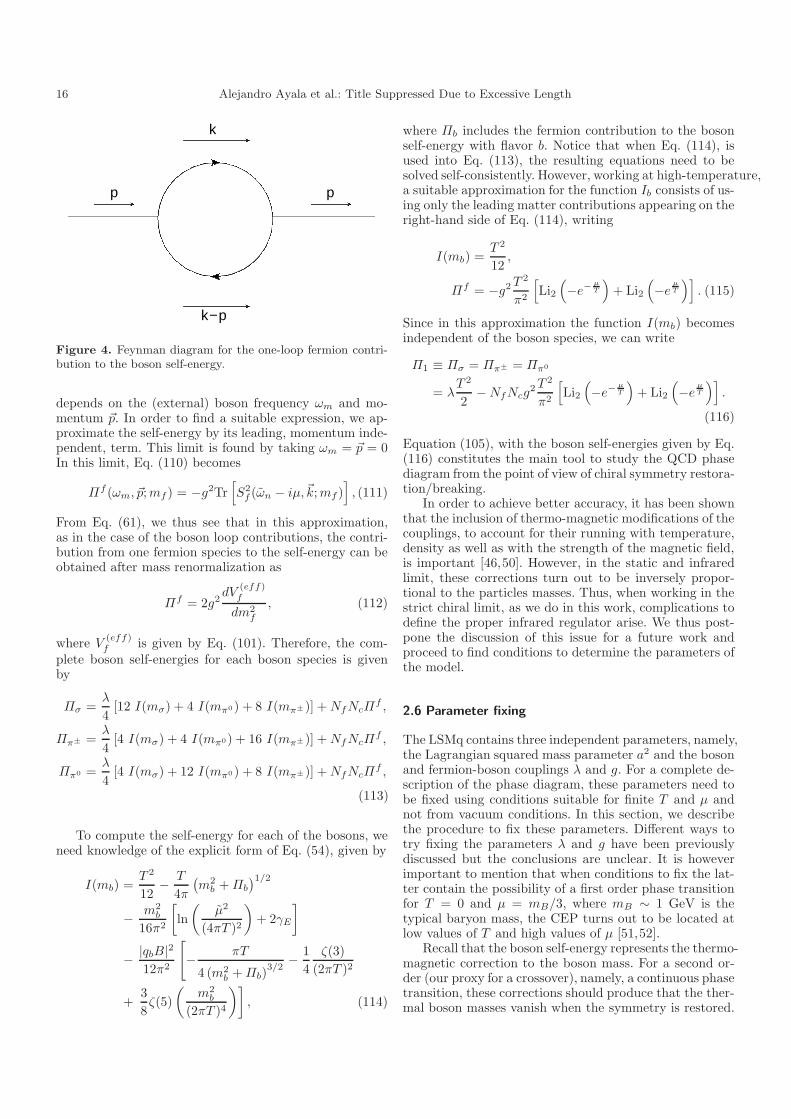
Figure 4. Feynman diagram for the one-loop fermion contri-bution to the boson self-energy.
depends on the (external) boson frequency ωm and mo-mentum ~p. In order to find a suitable expression, we ap-proximate the self-energy by its leading, momentum inde-pendent, term. This limit is found by taking ωm = ~p = 0In this limit, Eq. (110) becomes
Πf (ωm, ~p;mf ) = −g2Tr[
S2f (ωn − iµ,~k;mf )
]
, (111)
From Eq. (61), we thus see that in this approximation,as in the case of the boson loop contributions, the contri-bution from one fermion species to the self-energy can beobtained after mass renormalization as
Πf = 2g2dV
(eff)f
dm2f
, (112)
where V(eff)f is given by Eq. (101). Therefore, the com-
plete boson self-energies for each boson species is givenby
Πσ =λ
4[12 I(mσ) + 4 I(mπ0) + 8 I(mπ±)] +NfNcΠ
f ,
Ππ± =λ
4[4 I(mσ) + 4 I(mπ0) + 16 I(mπ±)] +NfNcΠ
f ,
Ππ0 =λ
4[4 I(mσ) + 12 I(mπ0) + 8 I(mπ±)] +NfNcΠ
f ,
(113)
To compute the self-energy for each of the bosons, weneed knowledge of the explicit form of Eq. (54), given by
I(mb) =T 2
12− T
4π
(
m2b +Πb
)1/2
− m2b
16π2
[
ln
(
µ2
(4πT )2
)
+ 2γE
]
− |qbB|212π2
[
− πT
4 (m2b +Πb)
3/2− 1
4
ζ(3)
(2πT )2
+3
8ζ(5)
(
m2b
(2πT )4
)]
, (114)
where Πb includes the fermion contribution to the bosonself-energy with flavor b. Notice that when Eq. (114), isused into Eq. (113), the resulting equations need to besolved self-consistently. However, working at high-temperature,a suitable approximation for the function Ib consists of us-ing only the leading matter contributions appearing on theright-hand side of Eq. (114), writing
I(mb) =T 2
12,
Πf = −g2T2
π2
[
Li2
(
−e− µT
)
+ Li2
(
−e µT
)]
. (115)
Since in this approximation the function I(mb) becomesindependent of the boson species, we can write
Π1 ≡ Πσ = Ππ± = Ππ0
= λT 2
2−NfNcg
2T2
π2
[
Li2
(
−e− µT
)
+ Li2
(
−e µT
)]
.
(116)
Equation (105), with the boson self-energies given by Eq.(116) constitutes the main tool to study the QCD phasediagram from the point of view of chiral symmetry restora-tion/breaking.
In order to achieve better accuracy, it has been shownthat the inclusion of thermo-magnetic modifications of thecouplings, to account for their running with temperature,density as well as with the strength of the magnetic field,is important [46,50]. However, in the static and infraredlimit, these corrections turn out to be inversely propor-tional to the particles masses. Thus, when working in thestrict chiral limit, as we do in this work, complications todefine the proper infrared regulator arise. We thus post-pone the discussion of this issue for a future work andproceed to find conditions to determine the parameters ofthe model.
2.6 Parameter fixing
The LSMq contains three independent parameters, namely,the Lagrangian squared mass parameter a2 and the bosonand fermion-boson couplings λ and g. For a complete de-scription of the phase diagram, these parameters need tobe fixed using conditions suitable for finite T and µ andnot from vacuum conditions. In this section, we describethe procedure to fix these parameters. Different ways totry fixing the parameters λ and g have been previouslydiscussed but the conclusions are unclear. It is howeverimportant to mention that when conditions to fix the lat-ter contain the possibility of a first order phase transitionfor T = 0 and µ = mB/3, where mB ∼ 1 GeV is thetypical baryon mass, the CEP turns out to be located atlow values of T and high values of µ [51,52].
Recall that the boson self-energy represents the thermo-magnetic correction to the boson mass. For a second or-der (our proxy for a crossover), namely, a continuous phasetransition, these corrections should produce that the ther-mal boson masses vanish when the symmetry is restored.
Alejandro Ayala et al.: Title Suppressed Due to Excessive Length 17
This work
LQCD
0.0 0.1 0.2 0.3 0 0.5 0.60.80
0.85
0.90
0.95
1.00
1.05
1.10
|e|/Mπ2
Tc/Tc0
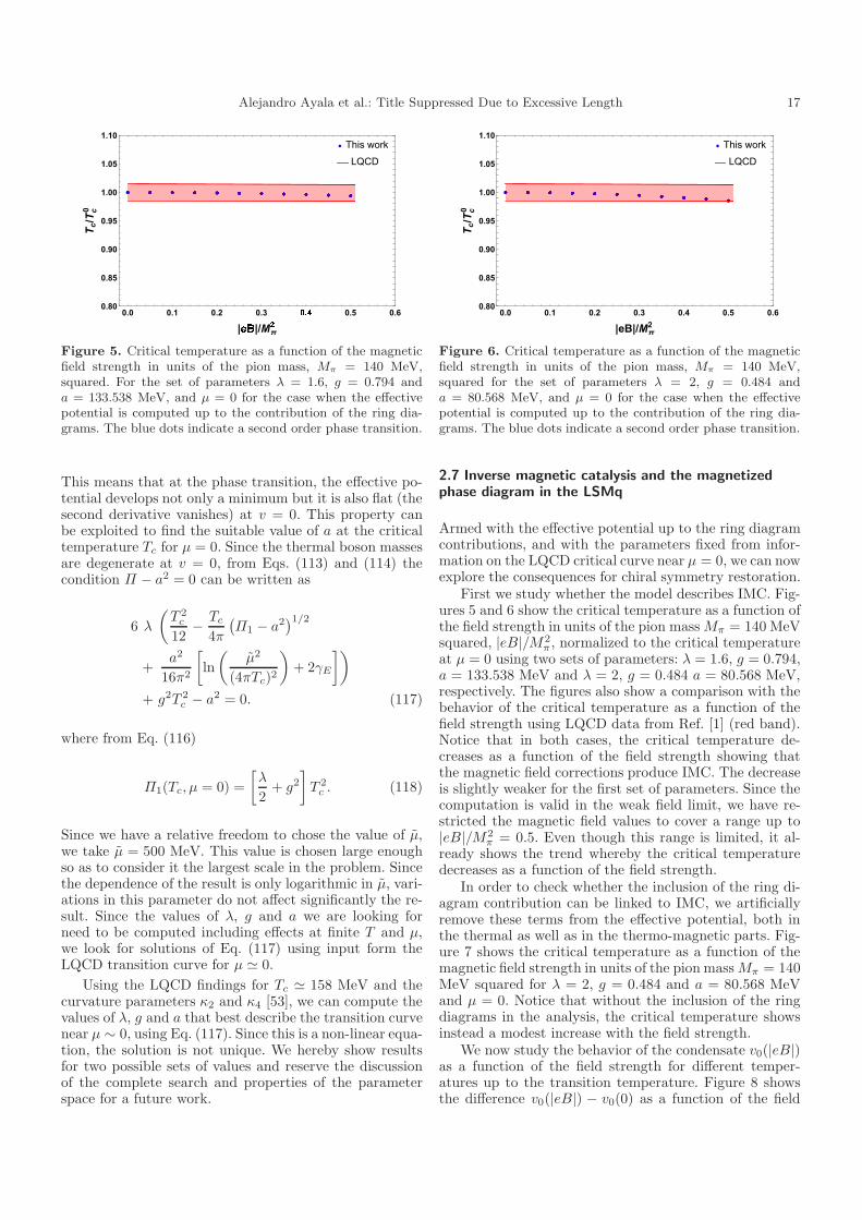
Figure 5. Critical temperature as a function of the magneticfield strength in units of the pion mass, Mπ = 140 MeV,squared. For the set of parameters λ = 1.6, g = 0.794 anda = 133.538 MeV, and µ = 0 for the case when the effectivepotential is computed up to the contribution of the ring dia-grams. The blue dots indicate a second order phase transition.
This means that at the phase transition, the effective po-tential develops not only a minimum but it is also flat (thesecond derivative vanishes) at v = 0. This property canbe exploited to find the suitable value of a at the criticaltemperature Tc for µ = 0. Since the thermal boson massesare degenerate at v = 0, from Eqs. (113) and (114) thecondition Π − a2 = 0 can be written as
6 λ
(
T 2c
12− Tc
4π
(
Π1 − a2)1/2
+a2
16π2
[
ln
(
µ2
(4πTc)2
)
+ 2γE
])
+ g2T 2c − a2 = 0. (117)
where from Eq. (116)
Π1(Tc, µ = 0) =
[
λ
2+ g2
]
T 2c . (118)
Since we have a relative freedom to chose the value of µ,we take µ = 500 MeV. This value is chosen large enoughso as to consider it the largest scale in the problem. Sincethe dependence of the result is only logarithmic in µ, vari-ations in this parameter do not affect significantly the re-sult. Since the values of λ, g and a we are looking forneed to be computed including effects at finite T and µ,we look for solutions of Eq. (117) using input form theLQCD transition curve for µ ≃ 0.
Using the LQCD findings for Tc ≃ 158 MeV and thecurvature parameters κ2 and κ4 [53], we can compute thevalues of λ, g and a that best describe the transition curvenear µ ∼ 0, using Eq. (117). Since this is a non-linear equa-tion, the solution is not unique. We hereby show resultsfor two possible sets of values and reserve the discussionof the complete search and properties of the parameterspace for a future work.
This work
LQCD
0.0 0.1 0.2 0.3 0.4 0.5 0.60.80
0.85
0.90
0.95
1.00
1.05
1.10
|eB|/Mπ2
Tc/Tc0
Figure 6. Critical temperature as a function of the magneticfield strength in units of the pion mass, Mπ = 140 MeV,squared for the set of parameters λ = 2, g = 0.484 anda = 80.568 MeV, and µ = 0 for the case when the effectivepotential is computed up to the contribution of the ring dia-grams. The blue dots indicate a second order phase transition.
2.7 Inverse magnetic catalysis and the magnetizedphase diagram in the LSMq
Armed with the effective potential up to the ring diagramcontributions, and with the parameters fixed from infor-mation on the LQCD critical curve near µ = 0, we can nowexplore the consequences for chiral symmetry restoration.
First we study whether the model describes IMC. Fig-ures 5 and 6 show the critical temperature as a function ofthe field strength in units of the pion massMπ = 140 MeVsquared, |eB|/M2
π , normalized to the critical temperatureat µ = 0 using two sets of parameters: λ = 1.6, g = 0.794,a = 133.538 MeV and λ = 2, g = 0.484 a = 80.568 MeV,respectively. The figures also show a comparison with thebehavior of the critical temperature as a function of thefield strength using LQCD data from Ref. [1] (red band).Notice that in both cases, the critical temperature de-creases as a function of the field strength showing thatthe magnetic field corrections produce IMC. The decreaseis slightly weaker for the first set of parameters. Since thecomputation is valid in the weak field limit, we have re-stricted the magnetic field values to cover a range up to|eB|/M2
π = 0.5. Even though this range is limited, it al-ready shows the trend whereby the critical temperaturedecreases as a function of the field strength.
In order to check whether the inclusion of the ring di-agram contribution can be linked to IMC, we artificiallyremove these terms from the effective potential, both inthe thermal as well as in the thermo-magnetic parts. Fig-ure 7 shows the critical temperature as a function of themagnetic field strength in units of the pion massMπ = 140MeV squared for λ = 2, g = 0.484 and a = 80.568 MeVand µ = 0. Notice that without the inclusion of the ringdiagrams in the analysis, the critical temperature showsinstead a modest increase with the field strength.
We now study the behavior of the condensate v0(|eB|)as a function of the field strength for different temper-atures up to the transition temperature. Figure 8 showsthe difference v0(|eB|) − v0(0) as a function of the field
18 Alejandro Ayala et al.: Title Suppressed Due to Excessive Length
0.0 0.1 0.2 0.3 0.4 0.5 0.6
157.6
157.8
158.0
158.2
158.4
|eB|/Mπ2
Tc[MeV]
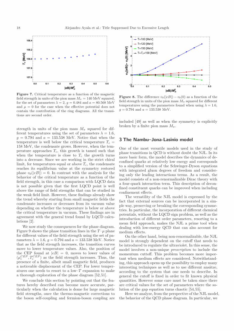
Figure 7. Critical temperature as a function of the magneticfield strength in units of the pion mass Mπ = 140 MeV squared,for the set of parameters λ = 2, g = 0.484 and a = 80.568 MeVand µ = 0 for the case when the effective potential does notcontain the contribution of the ring diagrams. All the transi-tions are second order.
strength in units of the pion mass Mπ squared for dif-ferent temperatures using the set of parameters λ = 1.6,g = 0.794 and a = 133.538 MeV. Notice that when thetemperature is well below the critical temperature Tc =158 MeV, the condensate grows. However, when the tem-perature approaches Tc, this growth is tamed such thatwhen the temperature is close to Tc the growth turnsinto a decrease. Since we are working in the strict chirallimit, for temperatures equal or above Tc, the condensatereaches its equilibrium value at the symmetry restoredphase v0(|eB|) = 0. In contrast with the analysis for thebehavior of the critical temperature as a function of thefield strength, in this case a comparison with LQCD datais not possible given that the first LQCD point is wellabove the range of field strengths that can be studied inthe weak field limit. However, these findings already showthe trend whereby starting from small magnetic fields thecondensate increases or decreases from its vacuum valuedepending on whether the temperature is below or abovethe critical temperature in vacuum. These findings are inagreement with the general trend found by LQCD calcu-lations [2].
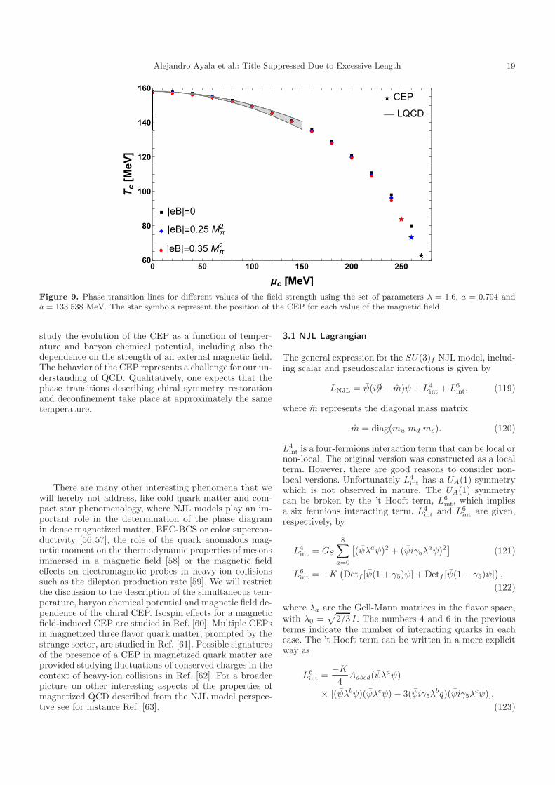
We now study the consequences for the phase diagram.Figure 9 shows the phase transition lines in the T –µ planefor different values of the field strength using the set of pa-rameters λ = 1.6, g = 0.794 and a = 133.538 MeV. Noticethat as the field strength increases, the transition curvesmove to lower temperature values. Also, the position ofthe CEP found at |eB| = 0, moves to lower values of(µCEPc , TCEPc ) as the field strength increases. Thus, thepresence of a finite, albeit small magnetic field, producesa noticeable displacement of the CEP. For lower temper-atures one needs to resort to a low–T expansion to makea thorough exploration of the phase diagram [52,51].
We conclude this section by pointing out that the fea-tures hereby described can become more accurate, par-ticularly when the calculation is dome for large magneticfield strengths, once the thermo-magnetic corrections tothe boson self-coupling and fermion-boson coupling are
T=100 [MeV]
T=120 [MeV]
T=150 [MeV]
T=Tc=158 [MeV]
0.0 0.1 0.2 0.3 0.4 0.5-2
0
2
4
6
8
|eB|/Mπ2
v0(|eB|)-v0(0)[MeV]
Figure 8. The difference v0(|eB|)− v0(0) as a function of thefield strength in units of the pion mass Mπ squared for differenttemperatures using the parameters found when using λ = 1.6,g = 0.794 and a = 133.538 MeV.
included [49] as well as when the symmetry is explicitlybroken by a finite pion mass Mπ.
3 The Nambu–Jona-Lasinio model
One of the most versatile models used in the study ofphase transitions in QCD is without doubt the NJL. In itsmore basic form, the model describes the dynamics of de-confined quarks at relatively low energy and correspondsto a simplified version of the Schwinger-Dyson equationswith integrated gluon degrees of freedom and consider-ing only the leading interactions terms. As a result, themodel consists of a non-renormalizable Dirac theory witha four-quark interaction term. This description of decon-fined constituent quarks can be improved when includingconfinement effects.
The versatility of the NJL model is expressed by thefact that external sources can be incorporated in a sim-ple way, preserving or breaking the corresponding symme-tries. In particular, the incorporation of different chemicalpotentials, without the LQCD sign problem, as well as theintroduction of different order parameters, resorting to amean field approach, makes the NJL a prime tool whendealing with low-energy QCD that can also account formedium effects.
On the other hand, being non-renormalizable, the NJLmodel is strongly dependent on the cutoff that needs tobe introduced to regulate the ultraviolet. In this sense, themodel involves a non-unique prescription to include themomentum cuttoff. This problem becomes more impor-tant when medium effects are considered. Notwithstand-ing, this approach opens up the possibility to employ manyinteresting techniques as well as to use different ansatze,according to the system that one needs to describe. Ingeneral the cutoff is fixed in order to fit known physicalquantities. However some care must be taken since thereare critical values for the set of parameters where the so-lution of the gap equation turns chaotic [54,55].
Here we analyze, from the perspective of the NJL model,the behavior of the QCD phase diagram. In particular, we
Alejandro Ayala et al.: Title Suppressed Due to Excessive Length 19
|eB|=0
|eB|=0.25 Mπ2
|eB|=0.35 Mπ2
CEP
LQCD
0 50 100 150 200 25060
80
100
120
140
160
μc [MeV]
Tc[MeV]
Figure 9. Phase transition lines for different values of the field strength using the set of parameters λ = 1.6, a = 0.794 anda = 133.538 MeV. The star symbols represent the position of the CEP for each value of the magnetic field.
study the evolution of the CEP as a function of temper-ature and baryon chemical potential, including also thedependence on the strength of an external magnetic field.The behavior of the CEP represents a challenge for our un-derstanding of QCD. Qualitatively, one expects that thephase transitions describing chiral symmetry restorationand deconfinement take place at approximately the sametemperature.
There are many other interesting phenomena that wewill hereby not address, like cold quark matter and com-pact star phenomenology, where NJL models play an im-portant role in the determination of the phase diagramin dense magnetized matter, BEC-BCS or color supercon-ductivity [56,57], the role of the quark anomalous mag-netic moment on the thermodynamic properties of mesonsimmersed in a magnetic field [58] or the magnetic fieldeffects on electromagnetic probes in heavy-ion collisionssuch as the dilepton production rate [59]. We will restrictthe discussion to the description of the simultaneous tem-perature, baryon chemical potential and magnetic field de-pendence of the chiral CEP. Isospin effects for a magneticfield-induced CEP are studied in Ref. [60]. Multiple CEPsin magnetized three flavor quark matter, prompted by thestrange sector, are studied in Ref. [61]. Possible signaturesof the presence of a CEP in magnetized quark matter areprovided studying fluctuations of conserved charges in thecontext of heavy-ion collisions in Ref. [62]. For a broaderpicture on other interesting aspects of the properties ofmagnetized QCD described from the NJL model perspec-tive see for instance Ref. [63].
3.1 NJL Lagrangian
The general expression for the SU(3)f NJL model, includ-ing scalar and pseudoscalar interactions is given by
LNJL = ψ(i/∂ − m)ψ + L4int + L6
int, (119)
where m represents the diagonal mass matrix
m = diag(mu md ms). (120)
L4int is a four-fermions interaction term that can be local or
non-local. The original version was constructed as a localterm. However, there are good reasons to consider non-local versions. Unfortunately L4
int has a UA(1) symmetrywhich is not observed in nature. The UA(1) symmetrycan be broken by the ’t Hooft term, L6
int, which impliesa six fermions interacting term. L4
int and L6int are given,
respectively, by
L4int = GS
8∑
a=0
[
(ψλaψ)2 + (ψiγ5λaψ)2
]
(121)
L6int = −K
(
Detf [ψ(1 + γ5)ψ] + Detf [ψ(1 − γ5)ψ])
,
(122)
where λa are the Gell-Mann matrices in the flavor space,with λ0 =
√
2/3 I. The numbers 4 and 6 in the previousterms indicate the number of interacting quarks in eachcase. The ’t Hooft term can be written in a more explicitway as
L6int =
−K4Aabcd(ψλ
aψ)
× [(ψλbψ)(ψλcψ)− 3(ψiγ5λbq)(ψiγ5λ
cψ)],
(123)

20 Alejandro Ayala et al.: Title Suppressed Due to Excessive Length
where the symmetric coefficientsAabcd are given byAabcd =13 ǫijkǫmnl(λa)im(λb)jn(λc)kl.
In addition to the interaction terms mentioned above,one can consider other chiral invariant operators, in partic-ular an interaction term involving vector and axial-vectorcurrents
L4V = GV
8∑
a=0
[
(ψγµλaψ)2 + (ψγµγ5λ
aψ)2]
. (124)
This term contributes only if finite density effects arepresent. It is easy to see that in the mean-field approx-imation, the relevant operator gives the quark density〈ψγµψ〉 = 〈ψ†ψ〉δµ0 [64]. Therefore, it is not possible toobtain GV a priori from known vacuum observables. GVmust be obtained using other in-medium phenomenologi-cal arguments.
3.2 Confinement
The NJL model does a good description of the dynamicsinvolving constituent quarks. However it lacks informationabout confinement. This information must be added andthere are different methods to include it. The most oftenused one is the inclusion of the Polyakov loop. Anothermethod is to consider non-local operators, and a third onecommonly used method is to consider an infrared cutoffconsidering the representation of the propagator in termsof a Schwinger proper-time [65].
The original version of the NJL model [66], includingquarks, has been used for the discussion of the phase tran-sition in the mean field approximation, where the quarkcondensate plays the role of the mean field for chiral sym-metry restoration. For a review on this subject, see Ref. [67].In this version of the model, the deconfinement transitionis absent. Perhaps, we should mention here that in prin-ciple these transitions are different in nature. Chiral sym-metry restoration is associated to a shift from a Nambu-Goldstone realization into a Wigner-Weyl realization. Inthe massless quark limit this is achieved by the vanish-ing of the quark condensate, the order parameter for thistransition, which can also be expressed in terms of the van-ishing of the pion decay constant. Deconfinement in thismodel can be taken into account through the Polyakovterm L(x), defined in terms of the trace of a Wilson loopin the Euclidean time direction
L =1
NcTrP exp
[
ig
∫ β
0
dτA0(x, τ)
]
, (125)
where g is the coupling in the QCD Lagrangian, Nc isthe number of colors in the theory and A0 = A0
aTa, with
T a the generators of SU(N). P denotes the path order-ing of the integral. The definition of this object is dueto Polyakov [68]. In the context of gauge theories at fi-nite temperature, this object provides an order parameterfor deconfinement. ’t Hooft [69] has highlighted the im-portance of the global symmetry Z(N) in gauge theories,
where Z(N) is the center of the group SU(N). In fact, forthe QCD Lagrangian we have the usual SU(Nc) transfor-mations Ω such that Dµ = Ω†DµΩ and ψ → Ω†ψ whereψ are the quark fields. Of course we have ΩΩ† = 1 andDetΩ = 1. If we consider a gauge transformation with aconstant phase multiplying the identity Ωc = e−iφINc×Nc
,in order for Ω to be an element of SU(N)c, the conditionDetΩc = 1 implies φ = 2πj/Nc with j = 0 · · · (N − 1).
Given the above condition, the expectation value ofthe Polyakov loop transforms in a non-trivial way un-der the center group ZNc
. If Φ = 〈L〉 we expect 〈L〉 =φ0 exp (i 2πj/Nc), where φ0 is a real function which shouldvanish for high temperatures. In fact, the expectation valueof the Polyakov loop corresponds to the ratio of the parti-tion functions of a system with an external quark insertedin a pure gluon system, ZQ, and the partition functionof a pure gluon system Z. i.e., ZQ/Z, from where we ob-tain Φ = 〈L〉 = exp (−βF ), where F is the free energyof the system with a single quark. For an external quarkinserted in a gluon system, this energy becomes infinityand therefore Φ = 0, which is tantamount of confinement.This means that one cannot have free color degrees offreedom in the system. On the contrary, for high temper-atures, since the theory becomes essentially free, 〈L〉 → 1.There must be an intermediate temperature where Φ goesbetween the confined and the deconfined phases. We seethat the expectation value of the Polyakov loop plays therole of an order parameter for deconfinement. Notice that,in the case of chiral symmetry restoration, the order pa-rameter is instead the quark condensate.
Let us now discuss the NJL model with a Polyakovterm, dubbed as the PNJL model. Let us start with theSU(3)f general NJL Lagrangian. The idea is to take intoaccount the vacuum expectation value of the trace of thePolyakov loop, Φ. We refer to this object as the Polyakovfield.
The idea is to build an effective potential U(Φ, Φ, T )such that the deconfinement transition is included. SinceΦ = 0 in the confined phase, this potential should have aminimum in Φ = 0 for T < T0. When T = T0 we expectthat Φ = 0 should correspond to a local maximum anda new minimum for Φ > 0 must appear triggering thedeconfinement phase transition through a breaking of theZ3 symmetry. This minimum will move to Φ = 1 when thetemperature grows beyond T0.
In the literature, several potentials satisfying these con-ditions have been proposed. The potential
1
T 4U(Φ, Φ, T ) = −a(T )
2ΦΦ+ b(T ) ln[1− 6ΦΦ
+ 4(Φ3 + Φ3)− 3(ΦΦ)2], (126)
where a(T ) = a0 + a1(T0/T ) + a2(T0/T )2 and b(T ) =
b3(T0/T )3 reproduces results from LQCD [70]. The pa-
rameters in this expression were fixed by comparing withLQCD data. They are given by: a0 = 3.51, a1 = −2.47,a2 = 15.2 and b3 = −1.75, where T0 is the critical tem-perature for a pure gauge field theory, which has beendetermined by LQCD as T0 = 270 MeV.
Alejandro Ayala et al.: Title Suppressed Due to Excessive Length 21
So far we have a NJL model for the quark sector anda potential for the Polyakov loop. This potential mimicsin some way the interacting gluons in QCD . The cou-pling between them is established through the covariantderivative Dµ = ∂µ − iAµ, where Aµ = gAaµ
λa
2 whereAaµ are the color gauge fields, i.e.. the gluons. Normallythe so called Polyakov gauge is used projecting the gaugefield in the 4th (Euclidean) component and parametriz-ing it diagonally as A4 = φ3λ
3 + φ8λ8, giving as a result
Φ = [cos(φ3/T ) + 1]/3.Certainly this model is not renormalizable and, at least
in its the local version, an ultraviolet cutoff is introducedas a sharp cutoff in three momentum space Λ. Several setsof values, with small variations for the parameters involvedin the model, have been used. For example in Ref. [71] wefind Λ = 631.4 MeV, mu = md = 5.5 MeV, ms = 135.7MeV, GΛ2 = 1.835 and KΛ5 = 9.29. See also Ref. [72].
Another perspective is obtained from the non-localversions of the NJL model (nlNJL). For a recent generalreference on the present status of non-local effective mod-els see Ref. [73]. There are some advantages with respectto the traditional local version which support these type ofmodels. For example, the inclusion of form factors, thatplay the role of non-local regulators, avoid dealing withthe problem of a sharp ultraviolet regulator Λ in momen-tum space. The precise value of Λ is a sort of instabilityin the predictions. As a second aspect, the presence of anon-local form factor in the scalar current js(x) leads to amomentum dependent quark effective mass, in agreementwith results form LQCD [74].
In the case of two flavors, the most simple nlNJL model,without ´t Hooft terms, corresponds to the Euclidean ac-tion
SE =
∫
d4x
ψ[−i/∂ +m]ψ −Gs[
(JS)2 + (JaP )
2]
,
(127)where the non-locality is encoded in the currents
JS(x) =
∫
d4zr(z)ψ(
x+z
2
)
ψ(
x− z
2
)
, (128)
JaP (x) =
∫
d4zr(z)ψ(
x+z
2
)
iγ5λaψ(
x− z
2
)
,
(129)
and where the regulator r(z) carries the effect of low en-ergy QCD interactions. Notice that we have chosen thesame form factor in both currents because of chiral sym-metry. If r(z) = δ4(z) we recover the local version of theNJL model. Several form factors have been used in the lit-erature, among which the most common one is the Gaus-sian regulator described in Euclidean momentum space asr(p2E) = exp(−p2E/Λ2), with Λ the cutoff already includedas the regulator.
3.3 Bosonization
Let us continue with the SU(2)f version of NJL withoutconfinement effects. The most simple expression for the
NJL Lagrangian that preserves chiral symmetry is
LNJL = ψi/∂ψ +G[
(ψψ)2 + (ψiγ5τψ)2]
, (130)
where the quark fields contain flavor and spin indexes, G isthe NJL coupling, and τ are the SU(2)f generators. ThisLagrangian is invariant under SU(2)L×SU(2)R transfor-mations.
The standard method used to obtain phase transitionsfor in-medium NJL is the minimization of the effectivepotential with respect of the different order parametersthat define the existence or not of a different phase.
There are many techniques that are used in order to ex-tract hadronic properties from the NJL Lagrangian, how-ever we focus only on the calculation of the effective poten-tial in the mean-field approximation. For these purposes,we then continue with the bosonization procedure.
The four-fermion operators can be transformed intoa quadratic fermion Lagrangian by the integration of aGaussian exponential, due to the introduction of auxiliaryfields. Then Eq. (130) for two flavors can be written as
eiSNJL = N∫
DσD3π eiSNJL[ψ,ψ,σ,πa], (131)
where SNJL =∫
d4xLNJL, and with the new quadratic-fermion action being
SNJL =
∫
d4x(
ψ[
i/∂ − σ − iγ5πaτa]
ψ
− 1
4G
[
σ2 + (πa)2]
)
, (132)
and where where N is some normalization constant. Withthe last step in mind, the NJL generating functional canbe written as the path integral of fermion fields and aux-iliary fields. The relation between bosons and fermionscomes implicitly from Eq. (132). By varying the bosonfields, the equations of motion give σ = −2G〈qq〉 andπa = −2G〈qiγ5τaq〉.
Since the new Lagrangian is quadratic with respect tothe fermion fields, they can be easily integrated out, andthe generating functional becomes expressed only in termsof the auxiliary fields
Z =
∫
DψDψ eiSNJL[ψ,ψ]
= N∫
DψDψDσD3π eiSNJL[ψ,ψ,σ,πa]
= N ′
∫
DσD3π eiSboson[σ,πa]
(133)
where the bosonic action is
Sboson = −iTr ln[i/∂ − σ − iγ5πaτa]
− 1
4G
∫
d4x[
σ2 + (πa)2]
, (134)
where the trace stands for spin, color, flavor, and configu-ration space. The generating functional is now represented

22 Alejandro Ayala et al.: Title Suppressed Due to Excessive Length
only by the scalar and pseudoscalar auxiliary fields whichcan be recognized as the sigma and pions, respectively.Considering an expansion around the mean field, by set-ting σ → 〈σ〉 + σ, πa → 〈πa〉 + πa, 〈σ〉 = σ 6= 0 and, inthe absence pion condensation, 〈πa〉 = 0, chiral symmetryis spontaneously broken.
Additionally we can break chiral symmetry explicitlyby adding a mass term to the original Lagrangian, namely,−mψψ. Considering the mean field approximation, we canobtain from Eq. (133) the effective potential Sboson[σ, π] →−V4Γ (σ), where the functional trace in momentum spacecan be written as
Γ = −iNfNc∫
d4p
(2π)4Tr ln(/p−m− σ) +
σ2
4G, (135)
and where the current quark mass term was introducedand the trace is over Dirac matrices. The value of themean field σ is obtained from the minimum of the effec-tive potential. The relation ∂Γ/∂σ = 0, produces the gapequation
2σ
G= NfNc
∫
d4p
(2π)4i(m+ σ)
p2 − (m+ σ)2 + iǫ, (136)
where we introduced the time-ordered regulator. The so-lution of the gap equation provides the value of σ as wellas the effective constituent mass of the quarksM = m+σ.
The introduction of the current quark mass allows usto obtain in a simple way the quark condensate. From thedefinition −iV4〈ψψ〉 = ∂ lnZ/∂m
〈ψψ〉 = −NfNc∫
d4p
(2π)4i(m+ σ)
p2 − (m+ σ)2 + iǫ(137)
so we can see, by comparing Eq. (136) with Eq. (137),that the quark condensate is related to the mean field σby the relation 〈ψψ〉 = −σ/2G.
The effective potential in Eq. (135), as well as the gapequation in Eq. (136), are UV-divergent. Since the the-ory is non-renormalizable, the regularization scheme pro-vides another parameter of the model and must be fixedin terms of physical quantities. The most often used onesare the regularization scheme and the momentum cutoff.Here we have three parameters: the coupling constant G,the mean field σ and the cutoff Λ. The gap equation fixesthe value of the mean field σ in terms of G and Λ, whichare in turn obtained calculating the pion mass and piondecay constant and fixing their values from their experi-mental ones. For a detailed description on the calculationof masses and decay constants see [64].
The different regularization schemes do not significantlychange the result of the chiral condensate, however, whenmedium effects are considered, the situation changes. Agood procedure is to regularize the vacuum part only,whenever possible. In principle there is no reason to as-sume that the cutoff or couplings must be independent ofmedium effects.
3.4 Temperature, chemical potential and magneticfield
The finite temperature effects can be easily introducedin the NJL model through the Matsubara formalism. Thesimplicity of this formalism translates itself into some min-imal replacements in the effective action, where now, V4Γ →−iβV Ω, with Ω the thermodynamical potential and β =1/T so that the generating functional in the mean-fieldapproximation can be expressed as Z = e−βV Ω. The 0-component of the momentum in Eq. (135) must be re-placed by fermionic Matsubara frequencies p0 → iωn =i(2n+ 1)πT and consequently, the p0 integral is replacedby the sum
∫
dp0 → 2πiT∑
n.To incorporate a chemical potential, we have to add
to the NJL Lagrangian the Lagrange multiplier times thenumber density operator LNJL → LNJL + µψ†ψ, whichis then expressed as a shift in the momentum /p → /p +µγ0 and consequently, within the Matsubara formalism,produces a shift in the Matsubara frequencies as ωn →ωn − iµ.
With all the above considerations, the thermodynam-ical potential reads as
Ω = 4NfNcT∞∑
n=−∞
∫
d3p
(2π)3ln[
(ωn − iµ)2 + p2 +M2]
+σ2
4G(138)
with a constituent mass given by M = m + σ. The gapequation can be obtained by minimizing the thermody-namical potential with respect to the mean field, ∂Ω/∂σ =0. Once the mean field value σ = σ∗(T, µ) is obtained, wecan also get the quark number density nq = −∂Ω/∂µ|σ=σ∗
and the pressure P = −Ωreg|σ=σ∗ , where the regularizedthermodynamical potential is obtained by subtracting themedium contribution Ωreg = Ω −Ω|T,µ=0.
The presence of an external magnetic field modifiesthe NJL Lagrangian by adding the electromagnetic vec-tor potential through the minimal coupling scheme, bysetting the term i∂µ → i∂µ + eAµ, where, for the caseof a uniform constant field B = Bz, the vector poten-tial reads as A = (0, 0,−Bx, 0) in the Landau gauge, orA = 1
2 (0, By,−Bx, 0) in the symmetric gauge.The main methods to deal with NJL under an exter-
nal magnetic field are: 1) the use of the wave functionand energy spectrum of the effective Lagrangian, 2) theSchwinger proper time method and 3) the Ritus method.The Schwinger method provides the fermion propagator inthe presence of the external field in Eq. (138). It is possi-ble to express the propagator in the form of a proper timeintegral that can be expanded in a power series of themagnetic field and can also be expanded as a Laguerreseries in terms of the Landau levels.
The three methods mentioned above provide the resultin terms of a sum over Landau levels. Since we are in a firstinstance calculating the thermodynamical potential at theone-loop level, this will not be affected by the Schwingerphase. As a result, the problem simplifies to the following

Alejandro Ayala et al.: Title Suppressed Due to Excessive Length 23
11
1
1
2
2
2
2
3
3
3
3
Figure 10. CEP from different authors using NJL models.Ref. [72] (circles) with eB = 0.195GeV2 (1), eB = 0.852GeV2
(2) and eB = 1.95GeV2 (3).Ref. [76] (squares) with eB = 0 (1), eB = 0.118GeV2 (2), andeB = 0.294GeV2 (3).Ref. [60] (diamonds) eB = 0 (1), eB = 0.392GeV2 for 〈uu〉 (2)and 〈dd〉 (3).Ref. [77] (triangles) with eB = 0 (1), eB = 0.00588GeV2 (2)and eB = 0.0157GeV2 (3).
rules: Once the trace is performed, the result depends onlyon the energy spectrum. The replacement of the energyfunction E(p) → El(pz) where the transverse momentumchanges as p2
⊥ → 2|eqB|l, and the integral in momentumspace also changes as
∫
d2p⊥ → |efB|∑∞l=0. The charge
ef stands for the respective quark charge eu = 2e/3 anded = −e/3. As a result, the thermodynamical potentialcan be written as
Ω =σ2
4G+ 4Nc T
|eB|2π
∞∑
n=−∞
∞∑
l=0
∑
f=u,d
(2− δl0)
×∫
dpz2π
ln[
(ωn − iµ)2 + p2z + 2|efB|l +M2]
.
(139)
In the case where a chemical potential is introduced,the contribution of the vector operator −GV (ψγµψ)2 inthe NJL Lagrangian turns out to be relevant, because themean field value of the vector current is related to thequark number density 〈ψ†ψ〉.
3.5 Critical end point
The calculation of the position of the CEP using the NJLmodel has been worked by several authors, however thisis not a simple task. The identification of the CEP is donebasically by looking at the evolution of the susceptibilities,or else, by means of looking at the shape of the thermo-dynamical potential in terms of the order parameter (seeRef. [75] for a different approach).
Figure 10 shows the CEP in the temperature vs. quarkchemical potential (µq = µB/3) for several values of themagnetic field, using different approaches within the NJLformalism, without including the vector-current interac-tion. Basically all of them present an increment of the
Figure 11. Magnetic evolution of the CEP from Ref. [31] con-sidering the PNJL model without IMC and a vector-currentcoupling GV .
critical temperature as well as a reduction of the criti-cal chemical potential as compared to calculations with-out a magnetic field. In Ref. [72] (circles) the authors usea SU(3)f NJL model. In Ref. [76] (squares) the authorsuse the SU(2)f version of NJL model. In Ref. [60] (dia-monds) the author considers also the SU(2)f NJL modelbut separating the magnetic evolution between u-quarksand d-quarks. Finally, in Ref. [77] (triangles) the authorsconsider the SU(2)f non-local NJL model with a Gaussianregulator. It is interesting to observe that non-local effectschange dramatically the location of the CEP position.
All the aforementioned works do not include the vector-current interaction term. However, this is an importantcontributions since its mean field is directly related withthe baryon density. Also, none of the used models, in theshape they are hereby presented, describe IMC. A bet-ter understanding of the evolution of the CEP needs toinclude confinement effects, IMC and the vector-currentinteraction. Concerning the evolution of the CEP in thePNJL extended model, it is extremely interesting to stressthat IMC, i.e. the fact that the critical temperature de-creases as a function of the magnetic field, both for the chi-ral restoration and the deconfinement phase transitions,can be achieved only if the coupling Gs acquires a de-pendence on the magnetic field [33,78,79,80]. This depen-dence was first introduced in Ref. [33]. Since there are nodata from LQCD for the running coupling αs(eB) thatcould inspire a possible Gs(eB), a fit given by Gs(ζ) =G0s(1 + aζ2 + bζ3)/(1 + cζ2 + dζ4), where ζ = eB/Λ2
QCD,
and a = 0.0108805, b = −1.0133 × 10⁻⁴, c = 0.02228,d = 1.854 × 10⁻⁴, was introduced after fitting the modelcritical temperature for chiral restoration T χc measured inLQCD at µB = 0 [78]. Using this effective, magnetic fielddependent coupling in the PNJL Lagrangian, it has beenshown that the critical temperatures for both transitionsdecrease with an increasing magnetic field strength.
For a comparison of different parametrizations of thecoupling G(T,B) and the conditions that must be consid-ered see Ref. [81].
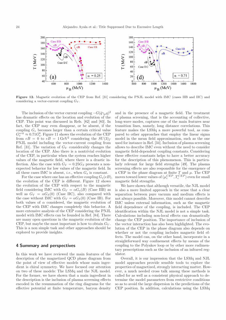
24 Alejandro Ayala et al.: Title Suppressed Due to Excessive Length
Figure 12. Magnetic evolution of the CEP from Ref. [31] considering the PNJL model with IMC (cases IIB and IIC) andconsidering a vector-current coupling GV .
The inclusion of the vector current coupling−G(qγµq)2has dramatic effects on the location and evolution of theCEP. This point was discussed in Refs. [82] and [83]. Infact, the CEP may even disappear, or be absent, if thecoupling Gv becomes larger than a certain critical valueGcritv ≈ 0.71G0
s. Figure 11 shows the evolution of the CEPfrom eB = 0 to eB = 1GeV2 considering the SU(3)fPNJL model including the vector-current coupling fromRef. [31]. The variation of GV considerably changes thelocation of the CEP. Also there is a nontrivial evolutionof the CEP, in particular when the system reaches highervalues of the magnetic field, where there is a drastic in-flection. Also the case with GV = 0.25GS presents a non-expected behavior for low values of the magnetic field. Inall these cases IMC is absent, i.e., when Gs is constant.
For the case where one has an effective couplingGs(eB),the evolution of the CEP is different. Figure 12 showsthe evolution of the CEP with respect to the magneticfield considering IMC with GV = αGs(B) (Case IIB) aswell as GV = αGS(0) (Case IIC), also compared withthe case without IMC with GV = αGS(0) (Case IB). Forboth values of α considered, the magnetic evolution ofthe CEP with IMC changes completely this behavior. Amore extensive analysis of the CEP considering the PNJLmodel with IMC effects can be founded in Ref. [84]. Thereare many open questions in the magnetic evolution of theCEP, but maybe the most important is how to obtain GV .This is a non simple task and other approaches should beexplored to provide insights.
4 Summary and perspectives
In this work we have reviewed the main features of thedescription of the magnetized QCD phase diagram fromthe point of view of effective models whose main ingre-dient is chiral symmetry. We have focused our attentionon two of these models: The LSMq and the NJL model.For the former, we have shown that a main ingredient inthe description is the inclusion of plasma screening effectsencoded in the resummation of the ring diagrams for theeffective potential at finite temperature, baryon density
and in the presence of a magnetic field. The treatmentof plasma screening, that is the accounting of collective,long-wave modes, captures one of the main features neartransition lines, namely, long distance correlations. Thisfeature makes the LSMq a more powerful tool, as com-pared to other approaches that employ the linear sigmamodel in the mean field approximation, such as the oneused for instance in Ref. [34]. Inclusion of plasma screeningallows to describe IMC even without the need to considermagnetic field-dependent coupling constants. Consideringthese effective constants helps to have a better accuracyfor the description of this phenomenon. This is particu-larly relevant for large field strengths [49]. The plasmascreening effects are also responsible for the emergence ofa CEP in the phase diagram at finite T and µ. The CEPmoves toward lower values of (µCEPc , TCEPc ) even for smallmagnetic field strengths.
We have shown that although versatile, the NJL modelis also a more limited approach in the sense that a clearseparation between pure vacuum and medium effects isnot always possible. Moreover, this model cannot describeIMC unless external information, such as the magneticfield dependence of the coupling, is included. The CEPidentification within the NJL model is not a simple task.Calculations including non-local effects can dramaticallychange the CEP position. The importance of inclusion ofthe vector interaction has also been highlighted. The evo-lution of the CEP in the phase diagram also depends onwhether or not the coupling includes magnetic field ef-fects. The model can, on the other hand, incorporate in astraightforward way confinement effects by means of thecoupling to the Polyakov loop or by other more rudimen-tary prescriptions such as the inclusion of an infrared reg-ulator.
Overall, it is our impression that the LSMq and NJLmodel approaches provide sensible tools to explore theproperties of magnetized, strongly interacting matter. How-ever, a much needed cross talk among these methods iscalled for as well as a consistent physical approach to de-termine the model parameters from restrictive conditionsso as to avoid the large dispersion in the predictions of theCEP position. In addition, calculations using the LSMq
Alejandro Ayala et al.: Title Suppressed Due to Excessive Length 25
are thoroughly worked out in the weak field limit whereasin the case of the NJL models equivalent calculations areperformed for strong fields. A possible avenue of encountercan be to work in one or the other limits using the corre-sponding model.
Acknowledgments
The authors are in debt to G. Endrodi for kindly sharingLQCD results for the critical temperature and condensateas functions of the field strength and to R. L. S. Fariasfor very useful conversations. The work was supported inpart by UNAM-DGAPA-PAPIIT grant number IG100219and by Consejo Nacional de Ciencia y Tecnologıa grantnumbers A1-S-7655 and A1-S-16215. M. L. acknowledgessupport from Fondecyt (Chile) regular grants No. 1200483and No. 1190192 and from ANID/PIA/Basal (Chile) un-der grant FB082. C.V. acknowledges financial support fromFONDECYT under grants 1190192 and 1200483.
References
1. G. S. Bali, F. Bruckmann, G. Endrodi, Z. Fodor, S. D.Katz, S. Krieg, A. Schafer, and K. K. Szabo. The QCDphase diagram for external magnetic fields. JHEP, 02:044,2012.
2. G. S. Bali, F. Bruckmann, G. Endrodi, Z. Fodor, S. D.Katz, and A. Schafer. QCD quark condensate in externalmagnetic fields. Phys. Rev. D, 86:071502, 2012.
3. G. S. Bali, F. Bruckmann, G. Endrodi, S. D. Katz, andA. Schafer. The QCD equation of state in backgroundmagnetic fields. JHEP, 08:177, 2014.
4. B. P. Abbott et al. GW170817: Observation of Gravita-tional Waves from a Binary Neutron Star Inspiral. Phys.
Rev. Lett., 119(16):161101, 2017.5. D. E. Kharzeev, L. D. McLerran, and H. J. Warringa.
The effects of topological charge change in heavy ion col-lisions:’Event by event P and CP violation’ . Nucl. Phys.
A, 803:227–253, May 2008.6. L. McLerran and V. Skokov. Comments about the elec-
tromagnetic field in heavy-ion collisions. Nucl. Phys. A,929:184 – 190, 2014.
7. Robert C. Duncan and Christopher Thompson. Formationof very strongly magnetized neutron stars - implications forgamma-ray bursts. Astrophys. J., 392:L9, 1992.
8. P. Esposito, N. Rea, and G. L. Israel. Magnetars: a shortreview and some sparse considerations. ArXiv e-prints,March 2018.
9. Alejandro Ayala, D. Manreza Paret, A. Perez Martınez,Gabriella Piccinelli, Angel Sanchez, and Jorge S.Ruız Montano. Kicks of magnetized strange quark starsinduced by anisotropic emission of neutrinos. Phys. Rev.
D, 97(10):103008, 2018.10. Tanmay Vachaspati. Magnetic fields from cosmological
phase transitions. Phys. Lett. B, 265(3):258 – 261, 1991.11. Jorge Navarro, Angel Sanchez, Maria Elena Tejeda-
Yeomans, Alejandro Ayala, and Gabriella Piccinelli. Sym-metry restoration at finite temperature with weak mag-netic fields. Phys. Rev. D, 82:123007, 2010.
12. Angel Sanchez, Alejandro Ayala, and Gabriella Piccinelli.Effective potential at finite temperature in a constant hy-permagnetic field: Ring diagrams in the standard model.Phys. Rev. D, 75:043004, 2007.
13. V. V. Skokov, A. Y. Illarionov, and V. D. Toneev. Estimateof the Magnetic Field Strength in Heavy-Ion Collisions.Int. J. Mod. Phys. A, 24:5925–5932, 2009.
14. Kirill Tuchin. Electromagnetic field and the chiral mag-netic effect in the quark-gluon plasma. Phys. Rev. C,91:064902, Jun 2015.
15. Lifang Xia, E. V. Gorbar, V. A. Miransky, and I. A.Shovkovy. Chiral asymmetry in cold qed plasma in a strongmagnetic field. Phys. Rev. D, 90:085011, Oct 2014.
16. Alejandro Ayala, C. A. Dominguez, L. A. Hernandez,M. Loewe, and R. Zamora. Magnetized effective qcd phasediagram. Phys. Rev. D, 92:096011, Nov 2015.
17. Alejandro Ayala, C. A. Dominguez, L. A. Hernandez,M. Loewe, Juan Cristobal Rojas, and Cristian Villavi-cencio. Quark deconfinement and gluon condensate in aweak magnetic field from qcd sum rules. Phys. Rev. D,92:016006, Jul 2015.
18. Alejandro Ayala, J. J. Cobos-Martınez, M. Loewe,Marıa Elena Tejeda-Yeomans, and R. Zamora. Finitetemperature quark-gluon vertex with a magnetic field inthe hard thermal loop approximation. Phys. Rev. D,91:016007, Jan 2015.
19. Alejandro Ayala, M. Loewe, and R. Zamora. Inverse mag-netic catalysis in the linear sigma model with quarks. Phys.Rev. D, 91:016002, Jan 2015.
20. Alejandro Ayala, Luis Alberto Hernandez, Ana JuliaMizher, Juan Cristobal Rojas, and Cristian Villavicen-cio. Chiral transition with magnetic fields. Phys. Rev.
D, 89:116017, Jun 2014.21. M. Loewe, C. Villavicencio, and R. Zamora. Linear sigma
model and the formation of a charged pion condensate inthe presence of an external magnetic field. Phys. Rev. D,89:016004, Jan 2014.
22. Alejandro Ayala, C. A. Dominguez, Saul Hernandez-Ortiz,L. A. Hernandez, M. Loewe, D. Manreza Paret, andR. Zamora. Thermomagnetic evolution of the QCD strongcoupling. Phys. Rev. D, 98(3):031501, 2018.
23. R. Hagedorn. Ultimate Temperature and the Structure ofElementary Particles. Prog. Sci. Culture, 1:395–411, 1976.
24. Larry McLerran and Robert D. Pisarski. Phases of cold,dense quarks at large N(c). Nucl. Phys. A, 796:83–100,2007.
25. A. Bazavov et al. Chiral crossover in QCD at zero andnon-zero chemical potentials. Phys. Lett. B, 795:15–21,2019.
26. Sayantan Sharma. The QCD Equation of state and criticalend-point estimates atO(µ6
B). Nucl. Phys. A, 967:728–731,2017.
27. A. Bazavov et al. The QCD Equation of State to O(µ6
B)from Lattice QCD. Phys. Rev. D, 95(5):054504, 2017.
28. A. Andronic, P. Braun-Munzinger, and J. Stachel. Hadronproduction in central nucleus-nucleus collisions at chemicalfreeze-out. Nucl. Phys. A, 772:167–199, 2006.
29. P. Braun-Munzinger, J. Stachel, and Christof Wetterich.Chemical freeze-out and the qcd phase transition temper-ature. Physics Letters B, 596(1-2):61–69, Aug 2004.
30. Gergely Endrodi. Critical point in the QCD phase diagramfor extremely strong background magnetic fields. JHEP,07:173, 2015.
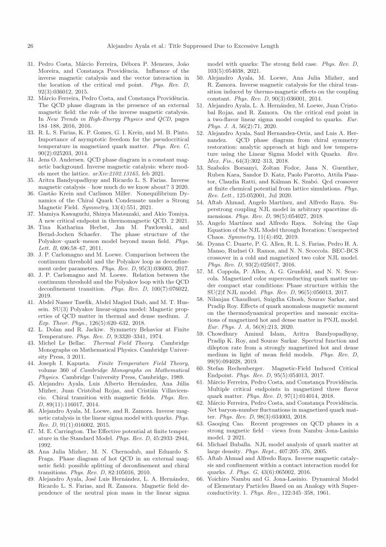
26 Alejandro Ayala et al.: Title Suppressed Due to Excessive Length
31. Pedro Costa, Marcio Ferreira, Debora P. Menezes, JoaoMoreira, and Constanca Providencia. Influence of theinverse magnetic catalysis and the vector interaction inthe location of the critical end point. Phys. Rev. D,92(3):036012, 2015.
32. Marcio Ferreira, Pedro Costa, and Constanca Providencia.The QCD phase diagram in the presence of an externalmagnetic field: the role of the inverse magnetic catalysis.In New Trends in High-Energy Physics and QCD, pages184–188, 2016, 2016.
33. R. L. S. Farias, K. P. Gomes, G. I. Krein, and M. B. Pinto.Importance of asymptotic freedom for the pseudocriticaltemperature in magnetized quark matter. Phys. Rev. C,90(2):025203, 2014.
34. Jens O. Andersen. QCD phase diagram in a constant mag-netic background. Inverse magnetic catalysis: where mod-els meet the lattice. arXiv:2102.13165, feb 2021.
35. Aritra Bandyopadhyay and Ricardo L. S. Farias. Inversemagnetic catalysis – how much do we know about? 3 2020.
36. Gastao Krein and Carlisson Miller. Nonequilibrium Dy-namics of the Chiral Quark Condensate under a StrongMagnetic Field. Symmetry, 13(4):551, 2021.
37. Mamiya Kawaguchi, Shinya Matsuzaki, and Akio Tomiya.A new critical endpoint in thermomagnetic QCD. 2 2021.
38. Tina Katharina Herbst, Jan M. Pawlowski, andBernd-Jochen Schaefer. The phase structure of thePolyakov–quark–meson model beyond mean field. Phys.
Lett. B, 696:58–67, 2011.39. J. P. Carlomagno and M. Loewe. Comparison between the
continuum threshold and the Polyakov loop as deconfine-ment order parameters. Phys. Rev. D, 95(3):036003, 2017.
40. J. P. Carlomagno and M. Loewe. Relation between thecontinuum threshold and the Polyakov loop with the QCDdeconfinement transition. Phys. Rev. D, 100(7):076022,2019.
41. Abdel Nasser Tawfik, Abdel Magied Diab, and M. T. Hus-sein. SU(3) Polyakov linear-sigma model: Magnetic prop-erties of QCD matter in thermal and dense medium. J.
Exp. Theor. Phys., 126(5):620–632, 2018.42. L. Dolan and R. Jackiw. Symmetry Behavior at Finite
Temperature. Phys. Rev. D, 9:3320–3341, 1974.43. Michel Le Bellac. Thermal Field Theory. Cambridge
Monographs on Mathematical Physics. Cambridge Univer-sity Press, 3 2011.
44. Joseph I. Kapusta. Finite Temperature Field Theory,volume 360 of Cambridge Monographs on Mathematical
Physics. Cambridge University Press, Cambridge, 1989.45. Alejandro Ayala, Luis Alberto Hernandez, Ana Julia
Mizher, Juan Cristobal Rojas, and Cristian Villavicen-cio. Chiral transition with magnetic fields. Phys. Rev.
D, 89(11):116017, 2014.46. Alejandro Ayala, M. Loewe, and R. Zamora. Inverse mag-
netic catalysis in the linear sigma model with quarks. Phys.Rev. D, 91(1):016002, 2015.
47. M. E. Carrington. The Effective potential at finite temper-ature in the Standard Model. Phys. Rev. D, 45:2933–2944,1992.
48. Ana Julia Mizher, M. N. Chernodub, and Eduardo S.Fraga. Phase diagram of hot QCD in an external mag-netic field: possible splitting of deconfinement and chiraltransitions. Phys. Rev. D, 82:105016, 2010.
49. Alejandro Ayala, Jose Luis Hernandez, L. A. Hernandez,Ricardo L. S. Farias, and R. Zamora. Magnetic field de-pendence of the neutral pion mass in the linear sigma
model with quarks: The strong field case. Phys. Rev. D,103(5):054038, 2021.
50. Alejandro Ayala, M. Loewe, Ana Julia Mizher, andR. Zamora. Inverse magnetic catalysis for the chiral tran-sition induced by thermo-magnetic effects on the couplingconstant. Phys. Rev. D, 90(3):036001, 2014.
51. Alejandro Ayala, L. A. Hernandez, M. Loewe, Juan Cristo-bal Rojas, and R. Zamora. On the critical end point ina two-flavor linear sigma model coupled to quarks. Eur.
Phys. J. A, 56(2):71, 2020.52. Alejandro Ayala, Saul Hernandez-Ortiz, and Luis A. Her-
nandez. QCD phase diagram from chiral symmetryrestoration: analytic approach at high and low tempera-ture using the Linear Sigma Model with Quarks. Rev.
Mex. Fis., 64(3):302–313, 2018.53. Szabolcs Borsanyi, Zoltan Fodor, Jana N. Guenther,
Ruben Kara, Sandor D. Katz, Paolo Parotto, Attila Pasz-tor, Claudia Ratti, and Kalman K. Szabo. Qcd crossoverat finite chemical potential from lattice simulations. Phys.Rev. Lett., 125:052001, Jul 2020.
54. Aftab Ahmad, Angelo Martınez, and Alfredo Raya. Su-perstrong coupling NJL model in arbitrary spacetime di-mensions. Phys. Rev. D, 98(5):054027, 2018.
55. Angelo Martınez and Alfredo Raya. Solving the GapEquation of the NJL Model through Iteration: UnexpectedChaos. Symmetry, 11(4):492, 2019.
56. Dyana C. Duarte, P. G. Allen, R. L. S. Farias, Pedro H. A.Manso, Rudnei O. Ramos, and N. N. Scoccola. BEC-BCScrossover in a cold and magnetized two color NJL model.Phys. Rev. D, 93(2):025017, 2016.
57. M. Coppola, P. Allen, A. G. Grunfeld, and N. N. Scoc-cola. Magnetized color superconducting quark matter un-der compact star conditions: Phase structure within theSU(2)f NJL model. Phys. Rev. D, 96(5):056013, 2017.
58. Nilanjan Chaudhuri, Snigdha Ghosh, Sourav Sarkar, andPradip Roy. Effects of quark anomalous magnetic momenton the thermodynamical properties and mesonic excita-tions of magnetized hot and dense matter in PNJL model.Eur. Phys. J. A, 56(8):213, 2020.
59. Chowdhury Aminul Islam, Aritra Bandyopadhyay,Pradip K. Roy, and Sourav Sarkar. Spectral function anddilepton rate from a strongly magnetized hot and densemedium in light of mean field models. Phys. Rev. D,99(9):094028, 2019.
60. Stefan Rechenberger. Magnetic-Field Induced CriticalEndpoint. Phys. Rev. D, 95(5):054013, 2017.
61. Marcio Ferreira, Pedro Costa, and Constanca Providencia.Multiple critical endpoints in magnetized three flavorquark matter. Phys. Rev. D, 97(1):014014, 2018.
62. Marcio Ferreira, Pedro Costa, and Constanca Providencia.Net baryon-number fluctuations in magnetized quark mat-ter. Phys. Rev. D, 98(3):034003, 2018.
63. Gaoqing Cao. Recent progresses on QCD phases in astrong magnetic field – views from Nambu–Jona-Lasiniomodel. 2 2021.
64. Michael Buballa. NJL model analysis of quark matter atlarge density. Phys. Rept., 407:205–376, 2005.
65. Aftab Ahmad and Alfredo Raya. Inverse magnetic cataly-sis and confinement within a contact interaction model forquarks. J. Phys. G, 43(6):065002, 2016.
66. Yoichiro Nambu and G. Jona-Lasinio. Dynamical Modelof Elementary Particles Based on an Analogy with Super-conductivity. 1. Phys. Rev., 122:345–358, 1961.
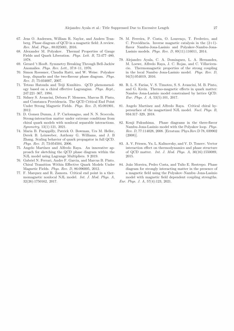
Alejandro Ayala et al.: Title Suppressed Due to Excessive Length 27
67. Jens O. Andersen, William R. Naylor, and Anders Tran-berg. Phase diagram of QCD in a magnetic field: A review.Rev. Mod. Phys., 88:025001, 2016.
68. Alexander M. Polyakov. Thermal Properties of GaugeFields and Quark Liberation. Phys. Lett. B, 72:477–480,1978.
69. Gerard ’t Hooft. Symmetry Breaking Through Bell-JackiwAnomalies. Phys. Rev. Lett., 37:8–11, 1976.
70. Simon Roessner, Claudia Ratti, and W. Weise. Polyakovloop, diquarks and the two-flavour phase diagram. Phys.
Rev. D, 75:034007, 2007.71. Tetsuo Hatsuda and Teiji Kunihiro. QCD phenomenol-
ogy based on a chiral effective Lagrangian. Phys. Rept.,247:221–367, 1994.
72. Sidney S. Avancini, Debora P. Menezes, Marcus B. Pinto,and Constanca Providencia. The QCD Critical End PointUnder Strong Magnetic Fields. Phys. Rev. D, 85:091901,2012.
73. D. Gomez Dumm, J. P. Carlomagno, and N. N. Scoccola.Strong-interaction matter under extreme conditions fromchiral quark models with nonlocal separable interactions.Symmetry, 13(1):121, 2021.
74. Maria B. Parappilly, Patrick O. Bowman, Urs M. Heller,Derek B. Leinweber, Anthony G. Williams, and J. BZhang. Scaling behavior of quark propagator in full QCD.Phys. Rev. D, 73:054504, 2006.
75. Angelo Martınez and Alfredo Raya. An innovative ap-proach for sketching the QCD phase diagram within theNJL model using Lagrange Multipliers. 9 2019.
76. Gabriel N. Ferrari, Andre F. Garcia, and Marcus B. Pinto.Chiral Transition Within Effective Quark Models UnderMagnetic Fields. Phys. Rev. D, 86:096005, 2012.
77. F. Marquez and R. Zamora. Critical end point in a ther-momagnetic nonlocal NJL model. Int. J. Mod. Phys. A,32(26):1750162, 2017.
78. M. Ferreira, P. Costa, O. Lourenco, T. Frederico, andC. Providencia. Inverse magnetic catalysis in the (2+1)-flavor Nambu-Jona-Lasinio and Polyakov-Nambu-Jona-Lasinio models. Phys. Rev. D, 89(11):116011, 2014.
79. Alejandro Ayala, C. A. Dominguez, L. A. Hernandez,M. Loewe, Alfredo Raya, J. C. Rojas, and C. Villavicen-cio. Thermomagnetic properties of the strong couplingin the local Nambu–Jona-Lasinio model. Phys. Rev. D,94(5):054019, 2016.
80. R. L. S. Farias, V. S. Timoteo, S. S. Avancini, M. B. Pinto,and G. Krein. Thermo-magnetic effects in quark matter:Nambu–Jona-Lasinio model constrained by lattice QCD.Eur. Phys. J. A, 53(5):101, 2017.
81. Angelo Martınez and Alfredo Raya. Critical chiral hy-persurface of the magnetized NJL model. Nucl. Phys. B,934:317–329, 2018.
82. Kenji Fukushima. Phase diagrams in the three-flavorNambu-Jona-Lasinio model with the Polyakov loop. Phys.Rev. D, 77:114028, 2008. [Erratum: Phys.Rev.D 78, 039902(2008)].
83. A. V. Friesen, Yu. L. Kalinovsky, and V. D. Toneev. Vectorinteraction effect on thermodynamics and phase structureof QCD matter. Int. J. Mod. Phys. A, 30(16):1550089,2015.
84. Joao Moreira, Pedro Costa, and Tulio E. Restrepo. Phasediagram for strongly interacting matter in the presence ofa magnetic field using the Polyakov–Nambu–Jona-Lasiniomodel with magnetic field dependent coupling strengths.
Eur. Phys. J. A, 57(4):123, 2021.