Finance and Economics Discussion SeriesDivisions of Research & Statistics and Monetary Affairs

Federal Reserve Board, Washington, D.C.

The Macroeconomic Effects of the Federal Reserve’sUnconventional Monetary Policies

Eric M. Engen, Thomas Laubach, and David Reifschneider

2015-005

Please cite this paper as:Engen, Eric M., Thomas Laubach, and David Reifschneider (2015). “The MacroeconomicEffects of the Federal Reserve’s Unconventional Monetary Policies,” Finance and EconomicsDiscussion Series 2015-005. Washington: Board of Governors of the Federal Reserve System,http://dx.doi.org/10.17016/FEDS.2015.005.

NOTE: Staff working papers in the Finance and Economics Discussion Series (FEDS) are preliminarymaterials circulated to stimulate discussion and critical comment. The analysis and conclusions set forthare those of the authors and do not indicate concurrence by other members of the research staff or theBoard of Governors. References in publications to the Finance and Economics Discussion Series (other thanacknowledgement) should be cleared with the author(s) to protect the tentative character of these papers.

Page 1 of 54  

The Macroeconomic Effects of the Federal Reserve’s  Unconventional Monetary Policies* 

 Eric Engen, Thomas Laubach, and Dave Reifschneider 

Federal Reserve Board January 14, 2015 

 

 

Abstract 

After reaching the effective lower bound for the federal funds rate in late 2008, the Federal Reserve turned to two unconventional policy tools—quantitative easing and increasingly explicit and forward‐leaning guidance for the future path of the federal funds rate—in order to provide additional monetary policy accommodation.  We use survey data from the Blue Chip Economic Indicators to infer changes in private‐sector perceptions of the implicit interest rate rule that the Federal Reserve would use following liftoff from the effective lower bound.  Using our estimates of the changes over time in private expectations for the implicit policy rule, and estimates of the effects of the Federal Reserve’s quantitative easing programs on term premiums derived from other studies, we simulate the FRB/US model to assess the actual economic stimulus provided by unconventional policy since early 2009.  Our analysis suggests that the net stimulus to real activity and inflation was limited by the gradual nature of the changes in policy expectations and term premium effects, as well as by a persistent belief on the part of the public that the pace of recovery would be much faster than proved to be the case.   Our analysis implies that the peak unemployment effect—subtracting 1¼ percentage points from the unemployment rate relative to what would have occurred in the absence of the unconventional policy actions—does not occur until early 2015, while the peak inflation effect—adding ½ percentage point to the inflation rate—is not anticipated until early 2016.      JEL classification: E5  Key words: federal funds rate, forward guidance, large‐scale asset purchases, monetary policy reaction function, zero lower bound           ____________________________ *The views expressed in this paper are those of the authors and do not necessarily reflect the views of others at the Federal Reserve Board or in the Federal Reserve System.  We thank Jim Clouse, Bill English, Refet Gürkaynak, Mike Kiley, David Lebow, Ed Nelson, and seminar participants at the European Central Bank and the Bank of France for helpful comments.     

Page 2 of 54  

I. Introduction  By the end of 2008, the Federal Reserve’s conventional monetary policy tool, the federal funds rate, was at its effective lower bound as the economy was in the midst of a financial crisis and deep recession.  In these circumstances, the Federal Open Market Committee (FOMC) turned to two unconventional policy tools—quantitative easing programs and increasingly explicit and forward‐leaning guidance for the future path of the federal funds rate—in order to provide additional monetary policy accommodation to help end the recession and strengthen the economic recovery.1  These unconventional policy actions were intended to put downward pressure on real longer‐term interest rates and more generally to improve overall financial conditions, including bolstering prices for corporate equities and residential properties.  More favorable financial conditions would, in turn, help boost aggregate demand and check undesirable disinflationary pressures by providing increased support for consumer spending, construction, business investment, and net exports.  A sizable number of studies have investigated the financial market effects of the FOMC’s unconventional actions, especially with regard to the Federal Reserve’s asset purchases, and found noticeable effects, on balance, on long‐term interest rates.2  By contrast, there have been relatively few studies of the effects of these actions on real activity and inflation, and this work has focused almost exclusively on macroeconomic effects arising only from the reductions in term premiums caused by large‐scale asset purchases.3  For these reasons, relatively little is known about the macroeconomic stimulus provided by the effects of the FOMC’s post‐crisis forward guidance and asset purchases on expectations for the future path of short‐term interest rates, nor how those expectational effects may have interacted with term premium shifts.  A central theme of this paper is that the two types of policy actions are highly interdependent, and that their macroeconomic effects thus need to be evaluated jointly.  In trying to gauge the macroeconomic effects of unconventional monetary policies since late 2008, we take into account the marked evolution over time of the public’s expectations for both future monetary policy and the overall economy; these factors, as our analysis will show, have an important bearing on the actual monetary policy stimulus provided by forward guidance and quantitative easing in recent years.                The next section of our paper provides a summary of the unconventional monetary policy actions taken by the Federal Reserve since late 2008.  The third section presents our methodology and assessment of how private‐sector expectations about monetary policy evolved from early 2009 through late 2013.  In particular, we use survey data from the Blue Chip Economic Indicators to infer the gradual changes that have taken place since early 2009 in private‐sector perceptions of the FOMC’s implicit policy rule—that is, the way in which short‐term interest rates would be adjusted in response to movements in real activity and inflation.  The fourth section discusses the other channel of the FOMC’s unconventional policy actions, the estimated effects of the Federal Reserve’s quantitative easing programs on the trajectories of the term premiums embedded in longer‐term interest rates.  With these estimates of expectational effects and term premium shifts in hand, we are in a position to score the actual stimulus 

                                                            1 Although forward guidance for the federal funds rate had been used in the past, policymakers still considered the nature of its recent use to be unconventional or nontraditional; see Bernanke (2012), for example. 2 These studies include Bauer and Rudebusch (2012), D’Amico, English, Lopez‐Salido and Nelson (2013), D’Amico and King (2013), Gagnon et al (2011), Hamilton and Wu (2012), Joyce and Tong (2013), Krishnamurthy and Vissing‐Jorgensen (2011), Li and Wei (2013), Meaning and Zhu (2011), Neely (2010), Rosa (2012), Rogers, Scotti and Wright (2014), and Swanson (2011). 3 These studies include Chen, Curdia, and Ferrero (2011), Chung et al (2012), Baumeister and Benati (2013), Gertler and Karadi (2013), and Weale and Wieladek (2014). 

Page 3 of 54  

to real activity and inflation provided by unconventional policy since early 2009, conditional on some model of the macroeconomy.  For this purpose we use the FRB/US model, whose properties are discussed in the fifth section.  The sixth section then summarizes results from counterfactual simulations of FRB/US designed to score the actual macroeconomic stimulus provided by the FOMC’s post‐crisis forward guidance and asset purchases; an important feature of this exercise is the use of alternative specifications of the model in order to address important uncertainties about the current dynamics of the economy.  We conclude with some observations about the potential implications of our analysis for the efficacy of monetary policy in the event the economy were to again experience a deep and prolonged slump.  Several key findings emerge from our analysis.  In the years following the recession and financial crisis, we find that private‐sector forecasters gradually came to perceive that the FOMC in the future would pursue a significantly more accommodative policy than they had anticipated at the start of the crisis, in the sense that they revised up markedly over time their estimate of the FOMC’s responsiveness to economic slack.  This change in public perceptions of the FOMC’s implicit policy rule—which we estimate put considerable downward pressure on real long‐term interest rates over time, over and above any effects associated with changes in the underlying outlook for real activity and inflation—presumably occurred in response to the Federal Reserve’s quantitative easing and increasingly forceful forward guidance for the federal funds rate.  Together with the downward pressure on term premiums associated with asset purchases, these expectational effects appear to have eased financial conditions appreciably relative to what they otherwise would have been, thereby providing appreciable support to the economic recovery over time.  However, our analysis also shows that the net stimulus to real activity and inflation was limited by the gradual nature of the changes in policy expectations and term premium effects, as well as by a persistent belief on the part of the public that the pace of recovery would be much faster than proved to be the case.   Partly for these reasons, and partly because of the inherent lags in the monetary transmission mechanism, our analysis implies that the macroeconomic effects of the FOMC’s past unconventional policy actions have probably yet to manifest themselves in full.  In particular, we estimate that the peak unemployment effect—subtracting 1.2 percentage points from the unemployment rate relative to what would have occurred in the absence of the unconventional policy actions—does not occur until early 2015, while the peak inflation effect—adding 0.5 percentage point to the inflation rate—is not anticipated until early 2016.  II. The Federal Reserve’s Unconventional Monetary Policies  After the federal funds rate reached its effective lower bound, the FOMC turned to the unconventional strategy of using both quantitative easing (QE) along with increasingly explicit and forward‐leaning guidance about the federal funds rate to provide additional policy accommodation.4  In the first part of this section, we provide a brief summary of how both approaches evolved over time.  After that, we review the general implications of these actions for financial market expectations and other factors.    

                                                            4 Other unconventional actions taken by the Federal Reserve during this period included several special credit programs that were intended to improve the functioning of financial markets, along with the introduction of macroeconomic “stress tests” for the largest banks to verify that they had sufficient capital.  Both programs probably helped to support economic activity during 2009 and early 2010 to some degree by enhancing the flow of credit and by increasing the public’s confidence in the banking system and the broader economy.  We have not tried to incorporate these programs into our analysis, however, because of the difficulties in accessing their effects using macroeconometric models.   

Page 4 of 54  

Summary of unconventional policy actions since late 2008  The FOMC’s QE programs were mostly comprised of large‐scale asset purchases (LSAPs) of longer‐term Treasury and agency mortgage‐backed securities (MBS), but also included the maturity extension program (MEP); the various stages of these QE policy actions are summarized in Table 1.  Cumulatively, the Federal Reserve’s holdings of Treasury notes and bonds along with agency MBS and agency debt rose from around $500 billion prior to the financial crisis to over $4 trillion when the most‐recent LSAP program concluded in October 2014.  The counterpart on the liability side of the Federal Reserve’s balance sheet was a substantial increase in its short‐term liabilities (primarily bank reserves).5  The LSAPs and MEPs materially lengthened the average duration of the securities held by the Federal Reserve, and thus reduced the average duration of Treasury and agency securities held by the public, relative to what otherwise would have occurred.6  As summarized in Table 2, the FOMC also began providing forward guidance for the future path of the federal funds rate in late 2008.  However, the initial guidance only advised that “weak economic conditions are likely to warrant exceptionally low levels of the federal funds rate for some time;” such limited guidance was not markedly different from that employed by the FOMC in 2003 and 2004.   Although the words “some time” were replaced by “an extended period” in early 2009, neither phrase provided the private sector with much specificity about either the likely date of liftoff of the federal funds rate or the economic conditions that would trigger it.  As a result, the public might have reasonably interpreted the guidance as consistent with the FOMC’s average historical behavior, given the severity of the recession and the projections of future real activity and inflation made at the time, rather than as signaling any intention of the FOMC to depart from its usual policy reaction function.  The specificity of forward guidance changed with the release of the August 2011 statement by the FOMC, in which the Committee noted that economic conditions would likely “warrant exceptionally low levels of the federal funds rate at least through mid‐2013”.7  The FOMC continued to issue similar calendar‐based guidance for roughly the next year and a half, although the cited dates were revised to “late‐2014” at the January 2012 meeting and to “mid‐2015” at the September 2012 meeting.  Such date‐based guidance helped financial market participants and others compare their expectations for the liftoff of the federal funds rate directly to those of the FOMC, and so had the potential to prompt revisions in the public’s expectations regarding the timing of liftoff and possibly the longer‐run conduct of monetary policy as well.  That said, such date‐based forward guidance was probably difficult for the 

                                                            5 The Federal Reserve did not hold any agency‐related debt and MBS as of late 2008 and held more than $200 billion in short‐term Treasury bills just before the recession.  By late 2014, the Federal Reserve did not hold any Treasury bills and had about $1.75 trillion in agency‐related securities and almost $2.5 trillion in Treasury notes and bonds.  The Federal Reserve had acquired about 19 percent of total federal Treasury debt held by the public when the most‐recent LSAP program concluded, only somewhat larger than the 15 percent share it held just prior to the last recession.  The Federal Reserve’s balance sheet expanded significantly because of the LSAP programs, but total federal debt held by the public also increased substantially from about 35 percent of GDP in 2007 to almost 75 percent of GDP in 2014. 6 The average duration of the securities held in the Federal Reserve’s portfolio increased from 1.6 years just prior to the most‐recent recession to 6.9 years near the end of 2014. 7 This guidance appeared to have been a surprise to financial market participants.  The event study by Femia, Friedman, and Sack (2013), for example, found that both longer‐term interest rates and the foreign exchange value of the dollar declined, while a broad index of U.S. equity values rose, immediately following this announcement of calendar‐based forward guidance by the FOMC.    

Page 5 of 54  

public to interpret because any differences between the FOMC’s liftoff guidance and private forecasts of liftoff could have reflected, at least in part, differences in forecasts for economic activity and inflation.    The FOMC eventually shifted away from calendar‐based guidance and adopted a more state‐contingent approach at the December 2012 meeting.  In that meeting’s statement, the FOMC announced that it would keep the federal funds rate at its effective lower bound “at least as long as the unemployment rate remains above 6½ percent, inflation between one and two years ahead is projected to be no more than a half percentage point above the Committee’s 2 percent longer‐run goal, and longer‐term inflation expectations continue to be well anchored.”  Subsequent FOMC statements released through late 2013 reiterated this guidance about the thresholds that would need to be crossed before the Committee would consider raising interest rates, while adding that the decision to tighten would also take account of broader labor market conditions and financial developments.  Another noteworthy change in forward guidance was made at the December 2013 meeting, when the Committee emphasized that the federal funds rate was likely to remain at its effective lower bound well past the time that the unemployment rate fell below 6½ percent, especially if inflation were to continue to run below its longer‐run target level of 2 percent and longer‐run inflation expectations remained stable.8    Of course, the forward guidance issued in FOMC statements was not the only way the Federal Reserve may have influenced policy expectations through its communications.  Among other communications that probably influenced the views of financial market participants and others in the private sector over the past few years were comments about the factors likely to influence future policy decisions made by individual FOMC participants in speeches, testimony, press conferences, and other forums; the FOMC’s regularly‐published Summary of Economic Projections with forecasts of the federal funds rate, economic activity, and inflation made by individual FOMC participants without attribution since January 2012; and the annual statements issued by the FOMC since January 2012 about its longer‐run goals and policy strategy.  In this regard, several speeches by Yellen (2012a,b,c) are worth highlighting because they emphasized that the FOMC’s guidance at the time about the likely date of liftoff was broadly consistent with the prescriptions of policies that were more accommodative than a standard Taylor‐type policy rule.  Indeed, Bernanke (2012) noted that changes to private‐sector forecasts appeared to reflect “a growing appreciation of how forceful the FOMC intends to be in supporting a sustainable recovery.”     Potential effects of unconventional policy actions  Both the QE programs and the forward guidance of the FOMC were intended to further help support economic activity and check undesirable disinflationary pressures after the federal funds rate had been lowered to its effective lower bound.  The QE policies were thought to put downward pressure on the general level of longer‐term interest rates primarily because they reduced the average duration of the Treasury securities and agency MBS held by the public, which in turn would cause the price charged by investors for lending over the longer run—the term premium—to decline.9  As a result, borrowing costs 

                                                            8 As a convenient cutoff point for our analysis, we consider the effects of FOMC unconventional policy actions taken through the end of 2013 only.  Our focus is on the macroeconomic effects of providing additional accommodation through unconventional policies.  With the announcement after the December 2013 FOMC meeting of the first reduction in the pace of asset purchases—implying, among other things, that downward pressure on term premiums would stabilize as the stock of the Federal Reserve’s long‐term securities holdings leveled out—we consider it unlikely that subsequent communications have sought to provide additional accommodation. 9 See Krishnamurthy and Vissing‐Jorgenson (2011), D’Amico, English, Lopez‐Salido, and Nelson (2012), and Li and Wei (2013) for discussions of this mechanism. 

Page 6 of 54  

for residential mortgages, auto loans, business borrowing, and other types of longer‐term lending would decline, all else equal; in addition, arbitrage effects imply that corporate equity prices and home values would rise and the real foreign exchange value of the U.S. dollar would decline.      By itself, forward guidance about future monetary policy need not provide monetary policy stimulus to the economy, especially if it merely confirms the public’s existing expectations for the central bank’s likely response to movements in economic activity and inflation over time.10  Rather, significant economic stimulus would require that financial market participants and others respond to the guidance by markedly altering their beliefs about future monetary policy in a more accommodative direction.  At issue, then, is whether the public interpreted the guidance provided by the FOMC since late 2008 as a credible signal that, as the economy recovered, the Federal Reserve intended to keep the federal funds rate lower for longer than would otherwise be expected given the FOMC’s historical responses to movements in resource utilization and inflation.11  If such a shift in public perceptions of the Federal Reserve’s implicit policy reaction function did in fact occur, then it should have caused expectations for the future path of short‐term interest rates to shift down and expectations for future inflation to move up, thereby putting downward pressure on real longer‐run interest rates in the near term even as the nominal federal funds rate remained stuck at its effective lower bound.  Allowing for arbitrage and spillover effects to other asset markets, this change in expectations could have helped to increase the value of corporate equities, real estate, and other forms of wealth, lower the real foreign exchange value of the dollar, and improve financial conditions more generally.      The Federal Reserve’s asset purchases also could have prompted shifts in policy expectations that stimulated the economy beyond what lower term premiums by themselves directly provided.12   Given the unprecedented magnitude of its quantitative easing programs, such asset purchases may have concretely and dramatically demonstrated the FOMC’s desire to provide additional accommodation, despite accompanying concerns by some about the effectiveness and potential costs of expanding the Federal Reserve’s balance sheet.  If so, the QE programs potentially boosted the credibility and hence effectiveness of the FOMC’s forward guidance by helping to convince financial market participants and others that the FOMC really would be persistently more aggressive than previously thought in using all its policy tools to bring the economy back toward full employment, while perhaps being more tolerant of a modest temporary overshoot in inflation as well.  Such shifts in policy expectations caused by the QE actions are extremely difficult, if not impossible, to disentangle from changes in expectations associated with forward guidance alone, given that both types of unconventional policies were used simultaneously and probably were mutually reinforcing.  For this reason, we estimate the macroeconomic effects of the combination of these two unconventional monetary policies.    

                                                            10 Of course, such confirmations might reduce uncertainty about the FOMC’s future behavior, and if by doing so, financial market participants, firms, and households became less concerned about potential risks to the outlook, then the clarifying of forward guidance could conceivably boost economic activity to some degree.    11 See Campbell, Evans, Fisher, and Justiniano (2012) for a discussion of the distinction between forward guidance that changes private expectations by publicly committing the FOMC to deviate from its usual policy reaction function—what they call “Odyssean” forward guidance—from forward guidance that may simply provide a forecast of future policy that only confirms the public’s expectations that the FOMC will follow its typical policy reaction function—what they call “Delphic” forward guidance. 12 In particular, this possibility has been noted by Bauer and Rudebusch (2011), Bhattarai, Eggertsson, and Gafarov (2014), and Woodford (2012). 

Page 7 of 54  

III. Measuring Shifts in Monetary Policy Rate Expectations  This section describes our procedure for estimating changes in private‐sector expectations about the way in which monetary policymakers were likely to respond to future movements in economic activity, inflation, and financial conditions.  To construct our estimates we use survey data from the Blue Chip Economic Indicators.  The co‐movements of the economic projections reported in the Blue Chip survey, together with the ways in which these forecasts have revised over time, allow us to infer how private‐sector forecasters’ beliefs about the FOMC’s implicit policy reaction function changed since late 2008.  In this regard, our methodology differs importantly from previous work such as Campbell et al. (2012), in that the typical approach has been to use survey data to infer expectations of temporary departures from “standard” central bank behavior (i.e., shocks to a fixed rule), rather than systematic changes to beliefs about how the central bank would respond to economic conditions.    For our purpose, the most informative survey results are those published every March and October, which include not only quarterly forecasts of economic activity, inflation, and interest rates for the current and coming year, which are collected every month, but also forecasts of annual conditions extending six years into the future.  Importantly, the March and October surveys also report forecasters’ assessments of conditions in the longer run, thereby allowing us to infer any changes over time in private assessments of the natural rate of unemployment, the equilibrium real rate of interest, and the FOMC’s effective inflation target, which are key parameters in the perceived policy reaction function.13  Figure 1 summarizes the evolution since 2007 of the Blue Chip consensus projections for the annual average of the 3‐month Treasury bill rate, the year‐over‐year rate of GDP price inflation, and the average annual unemployment rate, together with an imputed consensus forecast for the annual output gap.14  After the effective lower bound for the federal funds rate was hit in late 2008, private forecasters for some time projected that the Treasury bill rate would begin rising at a relatively rapid pace within a few quarters.  Starting in 2011, however, the projected liftoff date was pushed further into the future; in addition, the expected pace of tightening after liftoff declined appreciably while the nominal level of short‐term rates expected to prevail in the long run fell noticeably.  Presumably, these revisions in the expected path of short‐term interest rates are explained at least in part by marked revisions over time in the outlook for economic activity, as private forecasters gradually came to realize that the pace of recovery in the labor market and the broader economy would be markedly slower than initially anticipated in the immediate aftermath of the recession.  In contrast, revisions in the outlook for inflation published after March 2009 appear less substantial, with inflation always projected to converge relatively quickly back up to around 2 percent.  Given the recent average historical wedge between inflation measured using GDP prices and inflation measured using the PCE price index, the out‐year Blue 

                                                            13 Although the Blue Chip Economic Indicators reports updated projections each month, the forecast horizon for all but the March and October releases extends only to the coming year.  As a result, Blue Chip projections released in the other ten months of the year are of limited value in identifying shifts in private forecasters’ perceptions of the FOMC’s implicit reaction function, particularly as almost all forecasts released after early 2009 showed short‐term interest rates at their effective lower bound through most if not all of the following year.   14 Although the Blue Chip survey does not collect forecasts of the output gap, the ones published in March and October do report projections for the long‐run level of the unemployment rate—that is, the natural rate.  Private 

forecasters’ implicit projections for the output gap made at time t can thus be approximated as 2 ∗ , 

where  ∗denotes the consensus projection of the natural rate,   is the projected unemployment rate j years 

ahead, and 2 is the assumed value of the coefficient in Okun’s Law.  

Page 8 of 54  

Chip forecasts appear to be fairly well aligned with the longer‐term inflation objective of 2 percent (defined in terms of the PCE price index) that the FOMC announced in early 2012.15    In our model‐based evaluation of the quantitative effects of unconventional policies on real activity and inflation later in the paper, changes in public perceptions of the FOMC’s reaction function—presumed to be a direct consequence of the Federal Reserve’s forward guidance and asset purchases—are one of the two metrics of the “impulse” from unconventional monetary policy (the other being QE‐related shifts in term premiums).  To gauge the magnitude of changes in the perceived policy rule over time, we use the Blue Chip forecasts to infer private‐sector beliefs about the FOMC’s likely future responses to changes in economic conditions.  The historical behavior of the Federal Reserve and other central banks can be approximated quite closely by simple reaction functions, even if the policymakers at these institutions do not literally employ a rule to set the policy rate.16  Consistent with that evidence, it is reasonable to assume that, at time period t, private forecasters and others base their j‐step‐ahead expectations for short‐term interest rates on a Taylor‐type rule of the following form:  

(1)   ∗ ∗    

Here,  denotes the projected nominal short‐term interest rate,  ∗is the projected level of the real short‐term interest rate consistent with full employment over the longer run (i.e., the equilibrium real 

rate),  istheprojectedinflationrate, ∗is the perceived inflation target of the FOMC, and   is the projected output gap.  As noted above, the extended Blue Chip survey provides data on all the terms in this expression except the coefficients to be estimated—α and β—with the caveat that projections of the 3‐month Treasury bill rate must be used in place of forecasts of the expected federal funds rate; we think this is a reasonable substitution, given the high correlation between the two series. 17    As written, equation (1) allows for shifts over time in public perceptions of the FOMC’s responsiveness to movements in real activity and inflation. To provide a benchmark of private forecasters’ beliefs about the reaction function prior to the financial crisis, we estimate the parameters α and β over the period from the early 1990s, when the long‐horizon Blue Chip forecasts first become available, to the eve of the recession in 2007, treating both parameters as fixed coefficients in the context of a panel regression involving pooled Blue Chip consensus projections of varying horizons published at different times.  

                                                            15 The Blue Chip also reports consensus forecasts for the overall CPI, which might at first glance be thought of as more similar in nature to overall PCE prices—the FOMC’s preferred measure of inflation over the longer term—than the GDP price measure we use in our analysis.  However, in setting monetary policy, the FOMC has traditionally sought to look through temporary price fluctuations and instead focus on underlying inflation trends by, among other things, closely monitoring the generally more persistent movements in core PCE inflation as well as measures of long‐term inflation expectations.  Given the pronounced short‐run effects of transitory food and energy price fluctuations on the overall CPI, researchers have tended to use either core (CPI or PCE) inflation or GDP price inflation when estimating the FOMC’s reaction function.  The Blue Chip survey does not report forecasts for core inflation.  16 In particular, this behavior has been noted by Taylor (1993, 1999) and Taylor and Williams (2011).  17 In our analysis, the predicted value of the equilibrium real interest rate at time t is assumed to equal the long‐run Blue Chip forecast for the nominal Treasury bill rate less the long‐run projection for GDP price inflation.  Similarly, the perceived value of the FOMC’s inflation target is assumed to equal the long‐run projection for GDP inflation.  

Page 9 of 54  

Interestingly, the estimated parameters are very close to those suggested by the original Taylor (1993) rule.18  By contrast, one could plausibly expect the Federal Reserve’s unconventional policies over the past few years to have gradually altered public perceptions of the future responsiveness of the FOMC to changes in economic conditions.  Time‐varying perceptions of the FOMC’s response to economic conditions could take different forms; they could alter one or both of the response coefficients α and β, or they could have temporarily reduced the intercept of the perceived policy rule below the longer‐run 

equilibrium real rate  ∗.Given the emphasis placed on expected labor market conditions by the FOMC in its communications, we focus here on time variation in the economic slack parameter while keeping α fixed and setting the rule’s intercept to the survey‐implied long‐run equilibrium real rate.  In particular, one would expect the value of β consistent with the Blue Chip projections to rise over time.19    Accordingly, we do not pool results from different surveys in our regression analysis for the post‐recession period but instead estimate separate coefficients for each March and October survey released from 2009 through 2013.  Given that the surveys report annual projections for only the current year through six years ahead (plus an assessment of long‐run conditions), the number of observations employed in each individual regression is necessarily small.  To improve the degrees of freedom of this exercise, we fix the value of α in all the regressions at 0.5, its value in the standard Taylor rule and, as discussed above, consistent with the average behavior of the FOMC perceived by private forecasters in the years prior to the financial crisis.  Due to the comparatively minor deviations of inflation from the 2 percent objective, and the fact that these deviations were expected to close relatively quickly, allowing for time variation in the coefficient α would in any case not have had large effects on the expected future path of short‐term interest rates20  In light of the limited number of observations, we also do not consider temporary deviations of the intercept from the long‐run equilibrium real rate.  Table 3 summarizes the results from this regression analysis.  When annual projections at all published forecast horizons are included in the regression (the first column), the estimated coefficient on the output gap rises markedly over time, from less than 0.3 in the 2009 and 2010 surveys to more than 0.9 in the October 2013 survey.  However, the shift in the parameter estimates over time is biased downward since the near‐term annual projections of the Treasury bill rate in many of the surveys are constrained by the zero lower bound (ZLB), which causes the actual near‐term projections of short‐term interest rates to deviate from what the unconstrained policy rule would otherwise prescribe by an 

                                                            18 For example, in a pooled sample of all March and October Blue Chip surveys taken from 1992 through 2007, the estimated coefficients for α and β are .517 (.184) and .424 (.063), respectively.  (Standard errors in parentheses.)  In this regression, dummy variables are included for the zero‐step‐ahead forecasts to control for the fact that the observation partly reflects actual data.   19 In principle, perceived changes to monetary policy intentions could manifest themselves as anticipated future shocks to an unchanged FOMC implicit policy rule, in place of or in conjunction with changes in the rule’s coefficients.  In our analysis of the Blue Chip projections, however, we restrict ourselves to coefficient shifts for reasons of parsimony and because such shifts better capture the systematic changes in policy manifested in Blue Chip projections that extend six years into the future.  In contrast, Campbell et al (2012) use Blue Chip quarterly forecasts for the current and coming year to estimate shocks to an unchanged rule, possibly because their use of shorter‐horizon projections would not permit estimation of time‐varying policy rules.  20 For example, if the inflation coefficient in the perceived policy rule has remained about 0.5, then the marginal effect of the projected inflation gap on the Treasury bill rate is only on the order of 25 basis points on average in the first year of projections made since early 2009, with the effect diminishing rapidly with the extension of the forecast horizon thereafter. 

Page 10 of 54  

increasing amount over time.  To mitigate this problem, the second column of the table reports results when the regressions only include forecasts in which the projected Treasury bill rate is greater than 0.3 percentage point, a cut‐off point consistent with a federal funds rate above its current target range of 0 to 25 basis points.  (In practice, this screening involves dropping the current‐year and, in the later surveys, the one‐year‐ahead projections.)  In this case, the increase over time in the estimated value of β implicit in the consensus Blue Chip projections is even more pronounced, climbing from about 0.15 in the March 2009 survey to 1.60 in the October 2013 survey.  Based on these results, one could judge the effectiveness of the Federal Reserve’s unconventional policy actions in influencing policy expectations as considerable, particularly after the FOMC began issuing more explicit forward guidance in August 2011.    Figure 2 illustrates the implications for the projected trajectory of short‐term interest rates of these inferred shifts in the expected policy reaction function.  To begin, the black lines show the evolution of the actual Blue Chip projections of the Treasury bill rate published over the 2009‐2013 period, while the dashed red lines show what would have been prescribed by the standard Taylor (1993) rule conditional on the accompanying Blue Chip projections for economic slack, inflation, the equilibrium real rate, and the FOMC’s long‐run inflation target.  As the figure shows, private forecasters in early 2009 anticipated that short‐term interest rates would begin to rise much earlier and faster than predicted by the Taylor (1993) rule; this projected rapid tightening may have reflected forecasters’ belief that the FOMC would be reluctant to keep the funds rate at a level well below anything seen since the 1930s, even if such a low rate was consistent with perceptions of the FOMC’s past behavior as approximated by the Taylor rule.  This pattern persisted until October 2011, when the Blue Chip projections became reasonably well‐aligned with the standard Taylor rule.  After this date, private forecasters appeared to anticipate that the FOMC would be more patient than the standard Taylor rule implied for policy as the economy recovered, to a degree that increased appreciably over time.  The estimated changes in policy expectations underlying the Blue Chip projections is reasonably well approximated by the blue dashed line, which shows the policy prescriptions from a simple rule in which the perceived value of β revises over time as reported in the second column of Table 3, resulting—as one would expect—in much better tracking performance.    Nonetheless, the rules estimated with annual data have difficulty accounting for private forecasters’ expectations for the timing of liftoff as reported in both 2009 surveys and in the March 2010 and the March 2011 surveys.  These discrepancies, plus the emphasis placed in FOMC communications on the conditions that would warrant keeping the federal funds rate near zero, suggest taking a closer look at Blue Chip projections of unemployment and inflation at the time of liftoff, as is done in Table 4.  The first few columns of the table summarize the consensus forecasts for economic conditions in the quarter during which private forecasters implicitly expected the federal funds rate to first rise above its effective lower bound.21  In the immediate aftermath of the financial crisis, private forecasters anticipated that liftoff would occur in late 2009 even though the unemployment rate would still be above 9 percent and GDP price inflation would be only 1 percent.  As time passed, however, private forecasters pushed the 

                                                            21 Although the Blue Chip Economic Indicators survey does not publish funds rate projections, forecasts of the 3‐month Treasury bill rate can be used to infer the expected liftoff date.  In particular, the bill rate should equal the expected average value of the (overnight) federal funds rate over the next 91 days, abstracting from tax considerations and transitory safe‐haven effects.  Given that tax effects are essentially zero when the interest rates are very low, and given that safe‐haven concerns are presumed to be approximately normal when the Federal Reserve begins raising the federal funds rate target, we assume that if the projected T‐bill rate first rises above 0.3 percent in quarter t, then liftoff is expected to occur in quarter t+1.  As discussed in the appendix, this assumption appears reasonably consistent with financial market participants’ forecasts of the liftoff date for the federal funds rate.  

Page 11 of 54  

projected date for the onset of tightening further and further into the future, presumably in response to a disappointingly slow pace of recovery, continued moderate inflation, a sequence of large‐scale asset purchase programs, and increasingly aggressive forward guidance.  Critically, they revised down sharply their expectations for the rate of unemployment that would prevail at liftoff to about 6½ percent by late 2013, a level broadly consistent with the FOMC’s announced unemployment threshold, while gradually revising up their expectations for the accompanying rate of inflation to about 2 percent.22      Holding the value of α constant at 0.5, and assuming that the FOMC raises the federal funds rate to 50 basis points at liftoff, we can estimate the value of β consistent with the projections of economic conditions at liftoff (t=LO) in a specific Blue Chip forecast as:  (2) 0.5 ∗ 0.5 ∗ 2 ∗⁄   The final column of Table 4 reports the results from this calibration exercise using the projected values for the unemployment rate and inflation at liftoff reported in the second and third columns of the table and the long‐run Blue Chip forecasts for the unemployment rate, inflation, and the real funds rate reported in the fourth through sixth columns.  A comparison of these results with the final column of Table 3 reveals similar revisions in β over time.  For example, the implicit output gap coefficient at liftoff climbs from 0.25 in the March 2009 survey to 1.6 in the October 2013 survey, a change almost identical to that obtained using annual projections.  Moreover, most of the cumulative revision to β occurs after early 2011, as is the case with the annual estimates.  Finally, Figure 2 illustrates that, from the October 2011 survey on, the prescriptions of the estimated liftoff rules (dashed green lines) are quite similar to ones generated using the estimated annual rules (dashed blue lines).  Prior to that survey, however, it appears that private forecasters anticipated that the behavior of the FOMC would be noticeably more accommodative at the time of liftoff than it would be in the longer run.  (As in the case of the annual‐based estimates, the shifts in the expected sensitivity of the federal funds rate to slack at the time of liftoff would not be materially altered if we had instead assumed an accompanying decline in the coefficient on the inflation gap, given that private forecasters from October 2011 on consistently expected inflation to be close to its long‐run level at the time of liftoff.)  So far, we have made no allowance in our analysis for the possibility that private forecasters may have expected the FOMC to behave inertially, in that we have not included the lagged Treasury bill rate in our regressions as follows:  

(3)   1 ∗ ∗   

 

                                                            22 The Blue Chip forecasts released during 2013, after the initial announcement of thresholds, may in fact be more consistent with the FOMC’s forward guidance than implied by the estimates reported in Table 4 because the latter are affected by modest quarterly imputation errors beginning with the October 2011 release.  Beginning with that release, private forecasters anticipated that liftoff would occur sometime in the year following the coming year.  Because the Blue Chip survey provides quarterly forecasts for the current and coming year only, the exact quarterly timing of liftoff and its accompanying conditions in the October 2011 release and beyond must be imputed using annual projections.  These imputations are somewhat imprecise, particularly with regards to the federal funds rate, which is subject to the non‐linear effective lower bound and tends to be raised in discrete steps by the FOMC.  As a result, the liftoff date actually anticipated by private forecasters could be a quarter or two later than reported in the table, implying that the accompanying unemployment rate could be as much as ¼ percentage point lower.  The estimated inflation rate at the time of liftoff would be little changed, however. 

Page 12 of 54  

For forecasts published from 2009 through 2011, there appears to be little evidence of inertia.  For forecasts published from 2012 on, however, the story is somewhat different.  If λ is assumed  to equal 0.8 on a quarterly frequency, and β is calibrated as shown in the right‐most column of Table 3, then the resulting rule describes the Blue Chip forecasts about as well as the non‐inertial estimated rule.  The tracking performance of this calibrated rule is illustrated by the orange line in Figure 2.      There are several caveats to the results presented here.  First, our analysis assumes that private forecasters base their projections of short‐term interest rates on a simple policy rule involving only the output gap, inflation, and assessments of the equilibrium real rate and the FOMC’s inflation target.  In practice, however, their projections might incorporate other influences as well, such as the cyclical growth rate of real GDP, the health of financial institutions, or a perception that economy’s equilibrium real rate (the intercept in the rule) is time‐varying.  Second, our approximation for the projected output gap implicit in the Blue Chip survey could misstate private forecasters’ actual views about the likely trajectory for future resource utilization, as would occur if forecasters see the natural rate of unemployment as varying over the projection horizon and therefore not equivalent to their projections of the unemployment rate in the longer run, or if they anticipate variability in the Okun’s Law relationship perhaps, for example, related to unusual projected movements in trend labor force participation and trend productivity.  Third, even if our results do accurately gauge the evolution of the monetary policy views of private forecasters, those views may not conform closely to the views of households, firms, and the financial markets more broadly.  (As discussed in the appendix, however, forecasts made by financial market participants do seem broadly consistent with those published in the Blue Chip Economic Indicators.)    Nonetheless, we view the results as pointing strongly to a marked shift in the perceptions of private forecasters of the FOMC’s willingness to follow a highly accommodative monetary policy.  IV. Specifying the Effects of Federal Reserve Quantitative Easing on Term Premiums  In addition to estimating shifts in perceptions of the implicit policy reaction function, our analysis also needs to take into account the other monetary “impulse” from unconventional policy—the changes in term premiums associated with the Federal Reserve’s quantitative easing programs.  For estimates of these effects, we draw on the considerable body of work that has emerged in recent years concerning the financial market effects of large‐scale asset purchases.  Using a variety of techniques, a number of studies find on balance that the FOMC’s asset purchases have succeeded in reducing yields on longer‐term Treasury securities and agency MBS by an appreciable amount, and some have found noticeable reductions in corporate bond yields.23  In many of these studies, however, the reported reductions in yields may reflect a mix of changed expectations about the future path of short‐term interest rates and policy‐driven declines in term premiums.    For our analysis, we use the term premium estimates reported by Ihrig et al. (2012) because those estimates are derived using a methodology that allows the effects of shifts in term premiums on long‐term Treasury yields due to changes in quantitative easing policies to be isolated from other influences, including the effects of changes in expectations for the path of the federal funds rate.  Indeed, their results have several advantages over other research in this area.  To estimate the term premium effects 

                                                            23 These studies include Bauer and Rudebusch (2012), D’Amico, English, Lopez‐Salido and Nelson (2013), D’Amico and King (2013), Gagnon et al (2011), Hamilton and Wu (2012), Joyce and Tong (2013), Krishnamurthy and Vissing‐Jorgensen (2011), Li and Wei (2013), Meaning and Zhu (2011), Neely (2010), Rosa (2012), Rogers, Scotti and Wright (2014), and Swanson (2011); along with Kiley (2012) and Gilchrist, López‐Salido, and Zakrajšek (2014). 

Page 13 of 54  

of the quantitative easing programs, Ihrig et al rely heavily on the empirical arbitrage‐free term structure model developed by Li and Wei (2013).  This model presumes the existence of preferred‐habitat investors of the sort described by Vayanos and Vila (2009), which in turn implies that the slope of the yield curve should respond to supply factors such as changes in the size and maturity structure of the outstanding stock of Treasury and agency securities supplied to the public.24    Ihrig et al. adjust the methodology originally employed by Li and Wei to score the term premium effects of LSAP1 and LSAP2 by using the FOMC’s normalization plans announced in mid‐2011, which laid out the relationship between the timing of liftoff of the federal funds rate from the lower bound on the one hand, and the end of reinvesting maturing assets from the SOMA portfolio and the timing of asset sales on the other.  They combine this information with Blue Chip expectations for the timing of liftoff to arrive at market expectations for the path of the balance sheet.25  Ihrig et al. also employ the Li‐Wei methodology to score the effects of the maturity extension programs that the Federal Reserve initiated in September 2011 and completed in late 2012:  By reducing the average duration of the Treasury securities held by the public, MEP1 and MEP2 put further modest downward pressure on term premiums even as the size of the Federal Reserve’s portfolio remained unchanged. 26    Figure 3 plots the Ihrig et al. estimates of the term premium effects of the quantitative easing programs.  The black line indicates that the first round of asset purchases is estimated to have lowered the term premium on 10‐year Treasury yields roughly 40 basis points on average at the start of the program in early 2009.27  Thereafter, the term structure model predicts that the downward pressure on the term premium under the first LSAP program would be expected to diminish steadily as the average maturity of the Federal Reserve’s holdings declined, the scale of the economy increased, and the contemporaneous Blue Chip projections for the date of liftoff of the federal funds rate—which would signal the start of active balance‐sheet normalization—drew nearer.  As indicated by the green line, the 

                                                            24 Using monthly data from March 1994 through July 2007 on volumes and yields of Treasury securities and agency MBS, Li and Wei find strong empirical support for this theoretical proposition.  They also use their estimated model to infer the term premium effects of changes in the size and composition of public holdings of Treasury securities and agency MBS of the sort that resulted from the first two LSAP programs, and conclude that they were quite large. 25 Whereas Li and Wei’s estimates of the effects of the first two asset purchase programs were based on the assumption that the FOMC would begin selling assets two years after the end of each program and conclude such sales over a span of three years, Ihrig et al. tie the beginning of sales to the expected date of liftoff based on Blue Chip survey expectations, which at the time was expected to occur sooner than two years after the conclusion of each program, thereby reducing the term premium effects. 26 An assumption maintained throughout our analysis is that the Treasury did not change its strategy for the maturity composition of its issuance of new securities in response to the FOMC’s asset purchases.  The Treasury’s debt management strategy had been persistently increasing the average maturity of newly‐issued Treasury securities since around 2002.  Although the Treasury’s strategy had the opposite effect on the average duration of outstanding Treasury securities as the FOMC’s QE policies, the Treasury had begun to pursue its strategy long before the financial crisis and continued with it even with the FOMC’s decision to expand the size and duration of the Federal Reserve’s security holdings, which was consistent with the Treasury’s usual practice when faced with the large increases in federal government borrowing during this period.  Accordingly, the marginal effect of quantitative easing was still to reduce term premiums relative to what they otherwise would have been.  (See Greenwood, Hansen, Rudolph, and Summers (2014) for a more critical view of the Treasury’s debt management practice while the Federal Reserve was pursuing its QE programs.)   27 A portion of this effect occurs early in 2009 because the Federal Reserve made its first announcement about asset purchases at the very end of 2008.  The full scope of the first asset purchase program was not known until after the release of the FOMC statement in late March 2009. 

Page 14 of 54  

projected trajectory of term premium effects are estimated to shift down slightly with the FOMC’s announcement that payments on the Federal Reserve’s holdings of securities (particularly MBS) would be reinvested, slowing the rate of decline in the size and average duration of its portfolio.  Commencement of a second round of asset purchases in November 2010 is estimated to prompt a further downward revision in the projected path, which also incorporates the effects of the assets purchased under LSAP1 (solid red line).  Importantly, the initial revision in term premium effects at the start of LSAP2 is followed by further ones as Blue Chip forecasts for the date of liftoff are pushed further off into the future (the red dashed lines).  Finally, the Ihrig et al results indicate that the maturity extension programs first increased and then maintained the cumulative downward pressure on term premiums to about 60 basis through mid‐2012.  The three purple lines show the extension of the Ihrig et al. methodology to include the effects of the third round of asset purchases that began in September 2012.  The implementation of this program is estimated to have greatly magnified the downward pressure on term premiums, bringing it close to 120 basis points at the start of the program.  Market participants initially expected its size to be about $1.2 trillion, substantially smaller than the first asset purchase program; nonetheless its effects were substantially larger, in part because purchases of Treasury securities were concentrated in longer maturities than they had been in LSAP1, and in part because the expansion of the SOMA holdings was expected to last longer than the original purchases in 2009.  As shown by the first dashed line, the projected longer‐run trajectory of the cumulative effects from all asset purchase programs shifted down in response to FOMC communications indicating that it would probably eschew active sales of its MBS holdings once it began shrinking the size of its balance sheet, in contrast to the Committee’s previous guidance.  Finally, market expectations gradually shifted toward the program’s ultimate size of $1.5 trillion.  Because duration effects should vary across securities of different maturities, the results reported in Figure 3 apply only to the term premiums embedded in 10‐year Treasury yields.  Simulations of the Li‐Wei term structure model predict that the effects of the various asset purchase programs on the term premiums embedded in 30‐year Treasury yields should be on average only 35 percent or so of these estimated for 10‐year securities; the corresponding figure for 5‐year Treasury notes is about 80 percent.28    V. Estimating the Macroeconomic Effects of Unconventional Policies Using FRB/US  Having quantified the effects of the Federal Reserve’s unconventional policy actions on perceptions of its implicit policy rule and on term premiums, we now turn to the issue of the effects of these actions on aggregate economic activity and inflation over the past few years.  This section discusses our choice of a structural macroeconometric model for simulating the response of the economy to unconventional policy measures, and then presents and discusses results for some illustrative policy actions.     The FRB/US model  To quantify the macroeconomic effects of unconventional policies, we need a macroeconomic model that is structural in the sense that it can appropriately control for the effects of policy measures through expectations.  In fact, as our analysis will highlight, expectations about the future course of policy are critically important for the effectiveness of the unconventional policy actions 

                                                            28 We thank Min Wei for providing us with these figures. 

Page 15 of 54  

studied here.  While this general point has been appreciated since Lucas’ (1976) paper, this issue is of particular relevance in the circumstances of the past few years, when the public has had to rely disproportionately on policy announcements for forming expectations because there was no past record of unconventional policy actions at the ZLB to go by.  As mentioned earlier, only a few studies have examined the macroeconomic effects of unconventional policies in structural models.  These studies are mostly conducted using dynamic stochastic general equilibrium (DSGE) models built around a representative household and assuming some form of financial friction, such as in Chen et al. (2012) and Gertler and Karadi (2013).  In our study we use the Federal Reserve Board’s FRB/US model, which departs from these other models in certain dimensions that we will briefly discuss here.  More detailed information about the FRB/US model in general is available elsewhere.29  Three properties of FRB/US in particular are worth highlighting.  First, the FRB/US model features a broad array of financial assets whose prices can serve as potential transmission mechanisms for monetary policy: Besides the short‐term interest rate that is the (conventional) tool of monetary policy, there are long‐term Treasury securities at three different maturities, residential mortgages, corporate bonds, corporate equity, and the real trade‐weighted exchange rate.  The prices of these various assets are linked to each other via arbitrage conditions that include term and risk premiums which are themselves modeled as endogenous variables, depending in many instances on expectations about the future cyclical position of the economy.  In the baseline version of FRB/US used in this paper, term premiums are affected only by unconventional monetary policy measures, whereas risk premiums on other assets are endogenous.  The broad array of financial assets in FRB/US, and in particular the central role played by specific measures of long‐term interest rates, makes the model very useful for studying the effects of unconventional monetary policy, especially asset purchases.  That said, the reliability of its simulation results depends importantly on the empirical “reasonableness” of its predictions for QE‐related spillover effects on private borrowing rates, corporate equity prices, and the exchange rate—something that we will examine shortly.  From some perspectives, the approach taken in FRB/US may have certain limitations:  Practically all spending decisions depend on longer‐term real interest rates, thereby assigning equally strong effects on aggregate demand to changes in term premiums and in expected future short rates; and premiums are modelled in reduced‐form rather than being derived explicitly from financial frictions.30   A second feature is that there is no representative agent in the FRB/US model; instead there are both liquidity‐constrained and unconstrained households, where the former spend all their income each quarter and the latter consume and invest based on their assessment of their lifetime resources. In making this assessment, unconstrained households discount future labor and transfer income at a rate substantially higher than the discount rate on future income from non‐human wealth, reflecting uninsurable individual income risk.31  Notably, aggregate future income is valued 

                                                            29 Documentation of the model is available at www.federalreserve.gov/econresdata/frbus/us‐models‐about.htm, including a complete listing of model equations and coefficients, papers discussing different aspects of FRB/US, and illustrative simulation programs. 30 Kiley (2012) presents evidence that the aggregate demand effects of changes in term premiums may be weaker than those of expected future short rates. 31 The marginal propensity of households to consume out of different types of income can vary, depending on which group of households receives the income.  For example, transfer income is disproportionately received 

Page 16 of 54  

by different discount factors depending on its source and the average age of the recipient household.   As a result, the effective planning horizon for the average household in FRB/US is close to the five‐year period advocated by Friedman (1957) rather than the much longer time horizon of households embedded in a typical DSGE model.  This modeling choice reduces, in our view realistically, the ability to affect current economic activity through policies that raise expectations of future real activity and incomes (for example, as analyzed in Werning (2012)).  The absence of a representative household also means that we cannot evaluate unconventional policies according to their welfare implications; instead, we simply report their estimated effects on real economic activity and inflation.  Finally, price and wage inflation dynamics follow a New Keynesian Phillips curve specification in the presence of nonzero trend inflation.32  While this specification is very similar to those used in DSGE models, the estimated degree of inertia in price and wage inflation is higher than in most DSGE models based on the sticky‐price paradigm.  This feature interacts with households’ high discount rate of future income discussed before to dampen the effects of announced future monetary policy changes, such as forward guidance.  In particular, the combination of these two features explains why, as our results will show, the FRB/US model does not exhibit the “forward guidance puzzle” that besets standard DSGE models (Del Negro et al., 2013).33  As shown in Appendix 2, in a situation when the nominal short rate is held constant for an extended period of time, for example because the zero lower bound is binding, a credible announcement today of lower short‐term rates in the future raises current output and inflation in a canonical DSGE model, and these increases are larger the further into the future is the announced action.  Given constant nominal interest rates, the increase in inflation reduces current and expected future real interest rates, which in turn has strong aggregate demand effects because of the higher interest rate sensitivity due to households’ longer planning horizons.  Both of these channels are substantially and, in our view, plausibly attenuated in FRB/US.    Monetary policy is modeled as a simple rule for the federal funds rate subject to the zero lower bound on nominal interest rates; importantly for our analysis, the parameters of the policy rule used in simulations can be modified as desired to be consistent with private beliefs about the likely future behavior of the FOMC.  In our counterfactual simulations, the pronounced weakness of the economy since late 2008 means that the ZLB markedly and persistently constrains actual and expected monetary policy.  Moreover, the imposition of the ZLB makes the model highly non‐linear, thereby profoundly influencing the simulated dynamics of the economy.34    In our baseline version of the FRB/US model, all private agents are assumed to have rational expectations—that is, beliefs which are consistent with the dynamics of the full model, conditional on the anticipated behavior of policymakers.  The public does not necessarily have perfect foresight about 

                                                            by retirees who are well‐advanced in their lifecycles.  In addition, aggregation across age groups leads to average propensities to spend that vary across different types of aggregate income, reflecting variations in the distribution of income across groups. 32 The specification of the Phillips curve used in FRB/US is based on the model developed by Cogley and Sbordone (2008); this model allows for time variation in the underlying trend in inflation, reflecting (for the most part) changes in the central bank’s inflation objective.  In FRB/US, the post‐1979 trend is based on measures of expected long‐run inflation as reported initially in the Hoey Survey and later the Survey of Professional Forecasters. 33 See Chung (2015) for a comparison of the macroeconomic effects of forward guidance in the FRB/US model compared to two standard DSGE models. 34 To solve the model, we used the solution method described by Brayton (2012). 

Page 17 of 54  

the shocks that will hit the economy in the future, however, nor the FOMC’s response to those shocks.  While we view an examination of the effects of unconventional monetary policy in a range of alternative models as a worthwhile undertaking, it is beyond the scope of this paper.  Instead, we will report results of these effects for a range of alternative parameterizations of FRB/US, such as alternative assumptions about the formation of expectations by various agents, about inflation dynamics, and about the interest elasticity of aggregate demand.  Illustrative simulations  Before turning to estimates of the effects of the unconventional policy actions actually undertaken by the Federal Reserve, we illustrate the macroeconomic effects of forward guidance and asset purchases in a hypothetical scenario in which the U.S. economy is hit with a sequence of very large and persistent contractionary shocks.  In order to illustrate some key factors that influence the net stimulus provided by unconventional policy, and so need to be taken into account when we score the actual effectiveness of the FOMC’s actions in the next section, we run this exercise under alternative assumptions about both the public’s understanding of the persistence of the economic downturn and the speed at which policymakers respond.  The scenario is calibrated such that, under a baseline assumption of the federal funds rate following the standard Taylor rule and without any asset purchases, the federal funds rate is at its effective lower bound for five years.  Once the economic slump starts, the public is assumed to have perfect foresight about the shocks that will buffet the economy over time, as well as the monetary policy response to those shocks.  As indicated by the black lines in Figure 4, the magnitude of these shocks causes the unemployment rate to roughly double within the first two years, from 5¼ percent prior to the slump to a peak of 10¼ percent, and to decline thereafter gradually, while inflation drops by more than 1 percentage point.  Despite the associated decline in inflation expected over the next 10 years, the real 10‐year yield falls by about 2½ percentage points, reflecting the lower path of the real federal funds rate over that time horizon.  Because policymakers do not engage in large‐scale asset purchases in this scenario, term premiums are assumed to be unaffected although risk premiums on corporate bonds and equity increase endogenously.  As the red lines plotted in Figure 4 illustrate, these adverse effects would be noticeably mitigated by raising the output gap response coefficient from 0.5 to 1, which would delay liftoff from the effective lower bound by two quarters.  Thereafter, the federal funds path is little changed compared to the standard Taylor rule simulation, but given the higher path for inflation, the real 10‐year Treasury yield runs about ¼ percentage point lower for several years in a row.  Similar, albeit slightly smaller, effects from this change in policy rule obtain in a moderate slump scenario, in which the federal funds rate under the standard Taylor rule is constrained for only three years by the effective lower bound (the blue and green lines).  The marginal unemployment rate and inflation effects of various policy rule changes under these two scenarios are shown in Figure 5, expressed as deviations from outcomes under the standard Taylor rule.  In addition to the rule with an output gap coefficient equal to 1 (the red dashed lines), the figure also shows the effects of raising the output gap coefficient to 1.5, of raising it to 1.0 but in addition switching to an inertial rule with a coefficient of 0.8 on the lagged federal funds rate, or of implementing a threshold strategy whereby the federal funds rate stays at the effective lower bound until the unemployment rate falls below 6½ percent and thereafter follows the standard Taylor rule.  The macroeconomic effects of adopting either of these rules are larger in the highly persistent slump 

Page 18 of 54  

scenario (the left panels) than in the moderately persistent slump scenario (the right panels), and are the largest for the inertial rule, followed by the rule with an output gap response of 1.35  The first two columns of Table 5 provide information about the channels in FRB/US through which the change in the perceived policy rule is transmitted to real economic activity and inflation.  In the highly persistent slump scenario (the upper rows of the table), long‐term real Treasury yields decline mostly because of an increase in expected inflation rather than a reduction in the expected nominal path of future short‐term interest rates; the inflation effect is especially pronounced in the case of a change to an inertial policy rule (column 2).  Endogenous declines in risk premiums lead to larger reductions in real corporate yields as well as a notable increase in equity valuations.  Financial market effects are slightly smaller in the moderately persistent slump scenario, pointing to the importance of expectations about the persistence of adverse economic circumstances; differences from the highly‐persistent scenario would be more appreciable if the slump was even more transitory.   Figure 6 highlights the importance of informational assumptions for the estimated macroeconomic effects of these policies.  The left‐hand panels present the responses of unemployment and inflation under three of the rules that were reported in Figure 5, again expressed relative to outcomes under the standard Taylor rule without asset purchases, in the context of the highly persistent slump scenario.  As mentioned before, the public has a complete understanding of how the slump will develop over time, and monetary policy responds immediately to the crisis.  In contrast, the middle and right‐hand panels of the chart show the marginal effectiveness of the same policy initiatives under alternative assumptions for private agents’ knowledge of the future and the timing of policy responses.  Specifically, the middle panels of Figure 6 report the marginal effectiveness of the same shifts in policy rules when agents initially expect the contraction in real activity to be much less severe and persistent than actually turns out to be the case, and so only gradually come to understand that the economy has entered a prolonged ZLB episode.  The right‐hand panels of the figure show the stimulus provided when the public fully understands the nature of the shocks hitting the economy but the central bank shifts to a different policy rule only three years after the onset of the crisis, and the public does not anticipate any change in policy beforehand.  As can be seen, either type of delay not only shifts the timing of stimulus but actually reduces its magnitude—an important consideration in any scoring of the efficacy of the FOMC’s unconventional policy actions, given the gradual nature of the revisions to both the Blue Chip projections and policy expectations observed from early 2009 through late 2013.  Figure 7 shows the marginal effects of announcing a $1.5 trillion LSAP program at the onset of the crisis, conditioning on the interest rate rule in place at the time of the announcement.  Based on simulations of the Li‐Wei model, such a program would be expected to reduce the term premium embedded in the 10‐year Treasury yield about 60 basis points initially, with the effect fading away thereafter at roughly the average pace shown in Figure 3.  Columns 3 to 5 of Table 5 illustrate for three of the rules shown in Figure 7 that, in FRB/US, such a reduction in premiums directly increases the downward pressure on Treasury yields and indirectly influences other asset prices through arbitrage effects, thereby easing the cost of borrowing for households and firms, checking the recession‐driven declines in corporate equity valuations and household wealth, and further lowering the real foreign exchange value of the dollar.  

                                                            35 The simulation results are broadly consistent with the results reported in Tables 3 and 4.  In particular, in the middle column of Table 3, the estimated coefficient on the output gap rises above 1 in the March 2013 Blue Chip survey, when the unemployment rate at the time of liftoff is expected to be 6.8 percent.  By comparison, in the simulation in figure 5 with β equal to 1, the unemployment rate at the time of liftoff in the highly persistent slump scenario is 6.4 percent. 

Page 19 of 54  

For most of the rules, the marginal effects of the LSAP program are very similar.  The stronger economic conditions induced by the asset purchases call forth a stronger interest rate response after liftoff under the more‐aggressive policy rules, illustrating that in FRB/US, funds rate policy and asset purchases act to some extent as substitutes.  The anticipated reduction in the path of Treasury term premiums associated with asset purchases influences macroeconomic conditions via the former’s effects on a variety of financial market variables.  Except for the size of the term premium effect, which we take from the analysis of Ihrig et al. (2013), the financial market responses shown in Table 5 are endogenously generated by FRB/US.  Are the model’s predictions for the response of financial market conditions to a shift in Treasury term premiums in line with the empirical evidence?  In Appendix 2, we summarize some of the findings of event studies following QE‐related events.  Although there is some variety in results across studies, a good central estimate is that a QE‐induced reduction in 10‐year Treasury yields by 20 basis points is associated with a reduction in the 30‐year mortgage rate of about 25 basis points (reflecting the sizeable share of MBS purchases in the Federal Reserve’s QE programs), a reduction in BBB corporate bonds of about 15 basis points, an increase in equity prices of about 1¾ percent, and a reduction in the real exchange rate of about ¾ percent.  The relative magnitudes of the model‐generated responses shown in columns 3 to 5 of Table 5 are very close to these estimates, suggesting that the model provides a good approximation of this stage of the transmission channel.  The differences between the left and right panels in Figure 7 illustrate that the effects of LSAPs depend importantly on how long the federal funds rate is expected to remain at the effective lower bound, and hence how far into the future higher short‐term interest rates will begin to offset the effects of the LSAPs.  Accordingly, if agents at the launch of a QE program are substantially overestimating the pace at which the economy will recover and so project too early a date for liftoff of the funds rate, the direct downward pressure on long‐term interest rates caused by asset purchases initially will be substantially offset by a simultaneous upward revision to the expected path of future short‐term rates.  Similar considerations attend the stimulus provided by an announced change in the implicit policy rule.  If labor and product market gaps are already expected to close quickly even without the adoption of a more accommodative rule, then increasing the coefficient on slack or adopting a more inertial approach to policy setting will not markedly alter the projected future path of the funds rate, in contrast to what would occur if slack was expected to remain sizeable for many more years.  VI. The Effects of the FOMC’s Unconventional Policy Actions—Simulation Results  This section presents our quantitative assessments of the actual stimulus to real activity and inflation provided by the FOMC’s forward guidance and asset purchases since early 2009, based on counterfactual simulations of FRB/US.  We begin with a discussion of the design of our counterfactual simulation analysis, which among other things has to deal with complications arising from gradual learning on the part of the public about future monetary policy as well as the likely magnitude and persistence of the post‐crisis economic slump.  Using the baseline version of the model, we find that the FOMC’s unconventional policy actions apparently provided only a small boost to the real economy during the recession and the initial recovery period but that these effects have since become more substantial; the baseline counterfactual simulations also suggest that inflation effects to date have been relatively modest.  Considerable uncertainty attends these assessments, however, as simulations generated using plausible alternative specifications of the model yield a wide range of estimated unemployment and inflation effects; in addition, our analysis does not take into account the possibility 

Page 20 of 54  

that the FOMC’s unconventional actions may have led to marked improvements in household and business confidence, thereby significantly boosting the economy beyond what our model(s) predict.    Simulation design  To assess the consequences of announcing a systematic change in monetary policy, one typically starts with a baseline embodying some reference rule calibrated to match the FOMC’s recent behavior, and then simulates the effect of switching to a new policy rule under the assumption that agents have rational expectations and the policy announcement is completely credible.  As the preceding simulations demonstrate, however, the stimulus provided by unconventional policy at any point in time depended not on what the FOMC would actually do from that point forward, but on what the public at the time expected the Federal Reserve to do in the future—an important consideration for our efficacy assessments given that the perceived policy rule and the expected trajectory of term premium effects evolved gradually from early 2009 to late 2013.  Controlling for the pace of learning is also important with regards to changes over time in perceptions of the fundamental shocks acting to shape the economic outlook, given that the illustrative simulations also showed that the actual stimulus imparted by forward guidance and asset purchases partially depends on how long the funds rate is expected to remain constrained by the zero lower bound.  To control for these learning effects, we employ a sequence of baselines of past and projected conditions, each of which represents a snapshot of past economic developments and expectations for the future taken at a particular point in time.  This approach enables us to control for the actual timing of the shifts in expectations associated with revisions in both the perceived value of β in the implicit funds rate rule and the expected trajectory of QE‐related term premium effects.  In addition, it allows us to parse the forces driving changes over time in the economic outlook—as reflected in revisions to the extended Blue Chip projections—into those associated with perceived innovations in policy, and those associated with changing assessments of the fundamental shocks to aggregate demand and other factors hitting the economy, both now and in the past.    For computational convenience, we assume that expectations about future policy and other factors are updated twice a year, once in the first quarter to take on board on the information provided by the March Blue Chip surveys, and once in the third quarter to incorporate the results from the October surveys.  Each update of expectations requires the creation of a new baseline; thus, we construct a 2009Q1 baseline, a 2009Q3 baseline, a 2010Q1 baseline, and so on to our final 2013Q3 baseline.  The expected trajectory of QE‐related term premium effects incorporated into each baseline matches the corresponding path estimated by Ihrig et al and reported in Figure 3; for example, the path incorporated into the 2009Q3 baseline is the same as the LSAP1 path, while the path incorporated into the 2010Q3 baseline matches the initial estimated trajectory of LSAP2 effects.36 With regards to revisions in the policy rule across baselines, our base‐case assumption is that the perceived values of λ and α are always zero and 0.5, respectively, but that the perceived value of β guiding future monetary policy ratchets up markedly as one moves from the 2009Q1 baseline to the 2013Q3 baseline.  As discussed earlier, it appears that private forecasters persistently anticipated policy at the time of liftoff to be more accommodative than that which would be followed over the longer run.  Accordingly, we assume that 

                                                            36 The full dimensions of the first LSAP program were not announced until after the March 18, 2009 FOMC meeting, although some information about the Federal Reserve’s intentions to buy MBS was available in late 2008.  For this reason, we assume that agents in 2009Q1 expected asset purchases to lower term premiums by roughly 10 basis points in the first half of 2009, with the downward pressure eroding away rapidly thereafter. 

Page 21 of 54  

agents at the time of each survey expected β in the future to equal the values reported in Table 4 through the projected date of liftoff, but then anticipated that β would thereafter decline gradually to the longer‐run estimates reported in Table 3.  The precise pattern of revisions to the expected path of β across baselines is illustrated in Figure 8 by the rising sequence of black lines.  In addition to this base‐case assumption, we also consider an alternative evolution after 2011 for the perceived policy rule that is indicated by the red lines in the figure.  This alternative set of perceived paths for β, which are assumed to be accompanied by a jump in the perceived value of λ to 0.8, is consistent with our earlier finding that the Blue Chip Treasury bill rate forecasts published from this point are reasonably well explained by a smaller rise in β if they were accompanied by a perceived switch to inertial behavior on the part of the FOMC.    In addition to controlling for the timing of perceived changes in policy, our sequential baselines must also control for changes over time in views about the economic outlook and the underlying forces, past and projected, shaping it.  To do this, we start by generating an initial 2009Q1 baseline in which the paths for real GDP growth and several major spending components, the unemployment rate, inflation, interest rates, the natural rate of employment and other factors are forced to match the extended Blue Chip forecasts published in March 2009; this initial baseline also incorporates paths for the federal funds rate and term premium effects from quantitative easing that are consistent with private forecasters’ expectations in early 2009 for future monetary policy, including the anticipated date of liftoff.37  Next, we generate baselines corresponding to each subsequent Blue Chip forecast using a two‐step process.  The first step is to compute revised historical data for the new baseline; this is done by taking the baseline for the prior survey and adjusting its data for any revisions to real‐time published estimates of real GDP and other “headline” series that would have been available at the time the new Blue Chip survey was released.38  The second step is to run a constrained FRB/US simulation that hops off from the adjusted historical data and begins in the quarter that is assumed to correspond to the release date of the new Blue Chip survey; for example, the simulation start date would be 2009:Q3 in the case of the October 2009 survey and 2010:Q1 in the case of the March 2010 survey.  In each constrained simulation, we solve for the set of current and future shocks to aggregate spending, employment, supply‐side conditions, prices, and other factors that are needed to force the model under rational expectations to replicate the new extended Blue Chip projections.39  In solving for these anticipated shocks, the simulation conditions on the contemporaneous expectations for the date of liftoff, the future value of β, and the trajectory of QE‐related term premium effects discussed above.  This two‐step process is repeated until we have constructed baselines for 2009Q3 through 2013Q3.  

                                                            37 Beyond the end of the Blue Chip extended projection horizon, the 2009Q1 baseline (like all the subsequent ones) is assumed to converge gradually to a pre‐determined steady‐state growth path in which real GDP grows at its potential rate of 2¼ percent, the unemployment rate is flat at its natural rate of 5½ percent, PCE inflation equals the FOMC’s announced longer‐run objective of 2 percent, and the equilibrium real funds rate equals 2 percent.  Changing these steady‐state assumptions would have no effect on our estimates of the efficacy of unconventional monetary policy.  38 The adjustments to the historical data also include revisions to the model’s various expectational series, where the latter are computed to be consistent with the revisions to the published data and the dynamics of FRB/US. 39 Because the Blue Chip publishes forecasts for fewer variables than are in the model, no unique solution to this problem exists unless additional constraints are imposed on the allowable set of projection‐matching shocks.  We obtain a unique solution by imposing a variance‐covariance structure on the underlying shocks that is broadly consistent with the historical data; modest modifications to this structure would not have an appreciable effect on the results reported in the next section. 

Page 22 of 54  

Among other things, our baseline construction methodology parses the underlying forces driving the evolution of actual and expected economic conditions after early 2009 into two orthogonal parts—one part comprised of the sequence of perceived innovations to policy, and the other comprised of the sequence of revisions to past and projected shocks to aggregate spending and other fundamentals.  As a result, if one starts with the initial 2009:Q1 baseline, and then runs a sequence of unconstrained simulations whose starting points are progressively advanced in time (from 2009:Q3 through 2013:Q3), with each new simulation hopping off from the results of the prior simulation while incorporating a new set of revised shocks to fundamentals and policy (past and projected), then one replicates the real‐time evolution of both actual macroeconomic outcomes and the Blue Chip extended projections, with the final simulation exactly matching historical conditions and the Blue Chip outlook as they appeared in October 2013.  For our purposes, however, the more interesting exercise is to repeat these rolling simulations without incorporating the accompanying sequence of post‐2009Q1 revisions to liftoff dates, β paths, and the trajectory of expected term premium effects—that is, to re‐run history assuming no unconventional monetary policy innovations but allowing the same perceived shocks to other factors to unfold as they did.40  The difference between the actual evolution of the economy since 2009 and the course predicted by the counterfactual simulations of the sequence measures the actual stimulus provided by the FOMC’s forward guidance and asset purchases.  Baseline estimates  Figure 9 summarizes our baseline results, generated using the standard version of FRB/US assuming rational expectations on the part of all agents.  The black lines show the historical paths for real activity, inflation, and interest rates as they appeared in late 2013, extrapolated into the future using the extended Blue Chip projections published in October 2013.  The red lines, in contrast, show the predicted evolution of the economy after early 2009 had the FOMC not undertaken any unconventional policy actions, under the assumption that doing so would have caused the anticipated trajectory of QE‐related term premium effects and the perceived value of β in the implicit policy rule to remain unchanged at the paths expected in early 2009.  (The simulation does incorporate the modest QE‐related term premium effects anticipated in early 2009, equal to 10 basis points initially and fading rapidly thereafter.)  Beliefs about the past and projected shocks hitting the economy in the counterfactual simulation otherwise unfold over time as they did historically.  In the parsing exercises used to generate these historical shocks, the perceived evolution of the policy rule over history is the version in which the rule is assumed always to be non‐inertial.  In contrast, the blue lines of the figures show the predicted evolution of the economy in the absence of any unconventional policy actions when the parsing routine assumes that the perceived policy rule became inertial starting in 2012.  As can be seen, allowing for a shift toward inertial policy has little effect on the simulation results, presumably because such a shift (if it occurred) happened at a relatively late date and involved a smaller rise in the perceived value of β.  Three key points emerge from this analysis.  First, the model estimates that the FOMC’s unconventional policy actions provided essentially no stimulus in the first two years following the financial crisis, in that the simulation shows the unemployment rate peaking at the same level and real GDP growth and inflation essentially unchanged through 2010.  This early ineffectiveness is a result of several factors, including the relative modest changes to policy expectations that occurred during this period, initial 

                                                            40 In running these counterfactual simulations, we assume that the public always (correctly) anticipates that the federal funds rate in the starting quarter will remain at its effective lower bound but that the funds rate will strictly follow the prescriptions of the 2009:Q1 rule thereafter. 

Page 23 of 54  

beliefs that the economy would rebound more rapidly than proved to be the case, and inherent lags in the monetary transmission process.  However, there are reasons to think that this result understates the effectiveness of the early unconventional policy actions.  The first asset purchase program in particular is often credited with having greatly improved the functioning of key financial markets that had seized up during the most intense phase of the financial crisis.  In addition, the baseline model does not incorporate any mechanisms for the FOMC’s monetary policy actions to have affected such things as consumer confidence, business sentiment, and investors’ assessments of risks—extra‐model influences whose historical movements would manifest themselves in our parsing routines as shocks to spending, risk premiums, and other model variables.  If confidence and other extra‐model influences would have initially been even more impaired in the absence of asset purchases and forward guidance, then the counterfactual simulations may significantly understate their actual efficacy in 2009 and 2010.41      Second, the FOMC’s actions do appear to have appreciably sped up the pace of recovery beginning in 2011, with the model predicting a substantially slower decline in the unemployment rate after that point in the absence of forward guidance and asset purchases, accompanied by lower inflation.  Third, the model estimates that we are only now approaching the full effects of unconventional policy on real activity and inflation.  As indicated by the black lines of Figure 10, which show the difference between the actual evolution of the economy since early 2009 and that predicted by baseline model in the non‐inertial version of the counterfactual simulation, the peak unemployment effect—subtracting 1.2 percentage points from the unemployment rate—does not occur until early 2015, while the peak inflation effect—adding 0.5 percentage point to the inflation rate—is not anticipated until early 2016.  These estimates of the unemployment and inflation effects of the FOMC’s forward guidance and asset purchases are considerably smaller than the baseline estimates reported in Chung et al (2012) for just the term premium effects of LSAP1 and LSAP2, despite the fact that the latter’s estimates were also based on simulations of the FRB/US model.  Several factors account for the differences in estimated efficacy.  First, Chung et al based their term premium effects of LSAP1 and LSAP2 on the estimates reported in Gagnon et al (2011), which are twice as large as the Ihrig et al (2013) estimates employed in our study.  Second, Chung et al scored term premium effects holding the nominal federal funds rate fixed at its baseline path for the first five years, whereas the funds rate in our simulations always endogenously follows the prescriptions of a policy rule except when constrained by the ZLB, thereby greatly scaling back the net stimulus from asset purchases.  Third, our study controls for learning on the part of the public about the depth and persistence of the post‐crisis slump, whereas Chung et al implicitly assume that agents have perfect foresight about these conditions.  Finally, since the Chung et al study the FRB/US model has been reestimated and respecified, with the result that aggregate demand in the version used in this study is noticeably less interest sensitive; in addition, inflation is less sensitive to changes in current and expected economic slack.  Estimates derived from alternative model specifications  

                                                            41 Risk premiums on corporate bonds, equity, and the foreign exchange value of the dollar dropped appreciably more in the second quarter of 2009 than our parsing simulations can explain.  If we were to attribute all of these unexplained declines in risk premiums to the FOMC’s March 2009 announcement of an $1.75 trillion asset purchase program, on the grounds that this announcement demonstrated the Committee’s intention to do whatever it takes, then our estimates of the effects of unconventional monetary policy on real GDP growth would rise by ½ percentage point in both 2009 and 2010, even assuming that the declines in risk premiums would have occurred anyway over time. 

Page 24 of 54  

Considerable uncertainty obviously attends any estimate of the efficacy of the FOMC’s forward guidance and asset purchases.  Some of this uncertainty is associated with the shifts in policy expectations incorporated into our analysis:  Our estimates of the perceived changes to the policy rule implicit in private forecasts may be in error or may not reflect the beliefs of other economic agents, and the Li‐Wei model used to predict the trajectory of term premium effects from quantitative easing may be flawed.  And even if our estimates of the expectation effects of policy are reasonably accurate, the analysis of their macroeconomic implications may not be.  FRB/US is just one model, and other models may yield quite different results.  To this end, we now consider estimates of efficacy derived using several alternative specifications of the dynamics of the economy; among other things, this alternative analysis involves re‐running the construction of the sequential baselines and thus recalculating the perceived shocks (past and projected) hitting the economy over time.  We develop these alternative specifications by modifying key aspects of the structure of FRB/US rather than employing other structural models; in addition to being more convenient, we think this approach allows us to explore a wider range of plausible alternatives than could be done if we restricted ourselves to drawing the alternatives from the existing set of available DSGE models; this approach also allows us to analyze the macroeconomic effects of changes in the expected trajectory of term premium effects, something that most DSGE models cannot do.  That said, the limited set of alternative FRB/US specifications we consider below by no means spans the range of empirically‐relevant alternative characterizations of the dynamics of the economy.    Our first alternative involves the formation of expectations.  The assumption that all agents have rational expectations and fully understand the macroeconomic implications of forward guidance and asset purchases seems extreme, especially with regards to households who have at best a rather limited knowledge of such matters.  In addition, the empirical grounds for assuming rational expectations in household decision‐making, wage and price setting, and even business investment decisions is actually rather weak, despite the ubiquity of this assumption in modeling.  Accordingly, we consider an alternative version of FRB/US in which the only agents with rational expectations are financial market participants, an assumption that seems reasonable given their incentives to understand monetary policy.  Households and nonfinancial firms, in contrast, base their expectations for the future on the forecasts of small‐scale VAR models estimated using historical data, and so assume that the economy will display the same cyclical dynamics in the future that it did on average in the past.  Because these agents do not understand how unconventional policy alters those dynamics, forward guidance and asset purchases no longer directly cause households and non‐financial firms to mark up their expectations for real activity and inflation in the future, and so their initial stimulus falls.42  As indicated by the blue lines of Figure 10, the efficacy of the FOMC’s unconventional policy actions since early 2009 drops markedly under these assumptions, with a peak effect of reducing the unemployment rate by only 0.9 percentage points and almost no boost to inflation prior to 2014.    Our second alternative involves the dynamics of inflation.  Wages and prices in FRB/US are determined using an estimated New Keynesian Phillips curve.  The FRB/US empirical implementation of this model, however, yields inflation dynamics that are both more persistent and less sensitive to slack than that exhibited by many DSGE models.  Given the critical role played by inflation in the transmission channels of unconventional monetary policy at the zero lower bound, we therefore consider an alternative 

                                                            42 Households and nonfinancial firms do respond, however, to the (rational) changes in financial conditions that occur in response to such policy actions.  Note that the rationality of financial markets includes their knowledge that other agents in the economy do not have model‐consistent expectations.   

Page 25 of 54  

specification of the FRB/US wage‐price sector that brings its inflation dynamics into closer alignment with that embedded in these other models.43  As indicated by the red lines of Figure 10, making this change boosts the estimated peak effectiveness of the FOMC’s policy actions considerably, because the alternative specification predicts that asset purchases and forward guidance did considerably more to prevent a more marked (albeit transitory) disinflation from emerging over time.  That result, in turn, limited the rise in real short‐term interest rates that would have otherwise occurred in the face of the ZLB constraint, thereby providing additional support to real activity.     Our third alternative addresses the possibility that the interest sensitivity of aggregate demand is appreciably lower than predicted by the baseline model, particularly when allowance is made for some special factors that may have influenced the economy in the wake of the financial crisis.  In particular, tighter underwriting standards, impaired balance sheets, and an elevated level of uncertainty since early 2009 may have reduced the ability and/or willingness of households and firms to boost their spending in response to lower borrowing costs and increases in wealth.  To address this possibility, we create a low interest sensitivity model in which the responsiveness of consumer durable goods, residential investment, and business capital spending to movements in their respective costs of capital, and the responsiveness of stock prices and the real exchange rate to movements in long‐term Treasury yields, are half as large as in the baseline model.  As indicated by the green lines of Figure 10, allowing for such a pronounced constriction of the monetary transmission channels markedly reduces the estimated macroeconomic gains from forward guidance and asset purchases in this model.44  Our final alternative concerns the effects of the FOMC’s unconventional monetary policy on relative house prices.  In the baseline version of the model, movements in these prices are estimated to be essentially independent of changes in interest rates, real activity, and other macroeconomic factors.  Although this behavior is consistent with the historical time‐series behavior of house prices, the turn‐around in home values since their collapse in 2006‐2008 could have depended importantly on the support to housing market activity provided by extremely low mortgage rates.  If so, then the substantial pick‐up in actual and projected housing prices that has occurred since early 2009 might have been much weaker without forward guidance and asset purchases.  As shown in Figure 11, our sequential baselines 

                                                            43 In the baseline version of the FRB/US New Keynesian Phillips curve, current inflation depends upon (among other things) expected inflation in the next quarter, a weighted average of actual inflation over the past four quarters, and current labor market slack.  In the alternative version, the moving average of past inflation is replaced with a single lag and the coefficient on slack is increased by 50 percent.  Making these changes brings the dynamics of FRB/US at the zero lower bound into reasonably close alignment with those of EDO, the Federal Reserve Board’s estimated DSGE model of the U.S. economy.  44 Alternatively, the structure of the FRB/US model may overstate the influence of longer‐term interest rates on aggregate demand, and understate the role played by interest rates with a maturity of less than 5 years, leading to an overestimation of the stimulus provided by QE‐driven reductions in term premiums.  In this regard, Kiley (2013a) presents econometric evidence suggesting that the macroeconomic stimulus associated with historical shifts in term premiums is close to zero, perhaps because they do not induce the changes in borrowing costs, equity prices, and real exchanges rates predicted by the baseline version of the FRB/US.  Of course, Kiley’s findings may not be applicable to the recent QE‐driven shifts in term premiums for reasons related to identification, given that historical movements in term premiums were likely driven primarily by inflation uncertainty and flight‐to‐quality concerns, not policy; as a result, the past and present correlations of term premium shifts with real activity and inflation may be quite different.  When re‐running our analysis under the assumption of no pass‐through of QE‐driven term premium effects from Treasury securities to other asset prices, the peak effect of the FOMC’s unconventional policy actions on the unemployment rate and inflation drops to ‐0.7 percentage points and 0.2 percentage points, respectively.  

Page 26 of 54  

incorporate a substantial shift up over time in the actual and projected trajectories of house prices; these paths are constructed using real‐time data and surveys of expected changes in house prices for the current and coming year, extrapolated into the future using a simple trend‐reversion model of relative house prices.  In our final alternative scoring, we assume that actual and expected house prices in the absence of the FOMC’s unconventional policy actions would have followed the trajectory initially expected in early 2009 (the solid black line).  As indicated by the orange lines in Figures 10, under this assumption the estimated efficacy of the FOMC’s policy actions increases appreciably.  VII. Conclusions and Possible Implications for Future Monetary Policy  Several key findings emerge from our analysis.  In the years following the recession and financial crisis, we find that private‐sector forecasters pushed their expected time for the onset of tightening of monetary policy progressively further into the future, presumably in response to the Federal Reserve’s quantitative easing and increasingly aggressive forward guidance for the federal funds rate, in the context of a slow economic recovery with moderate inflation.  Although the Federal Reserve’s quantitative easing program likely helped to stabilize the economy during the financial crisis as it provided liquidity in financial markets that were seizing up, we estimate that the FOMC’s unconventional policy actions provided no material additional monetary policy stimulus in the first two years following the financial crisis, probably reflecting the relative modest changes to policy expectations that occurred during this period, anticipation that the economy would rebound more rapidly than proved to be the case, and the inherent lags in the transmission of monetary policy; a failure on the part of the FRB/US model to capture important confidence effects associated with unconventional policy could, however, significantly bias down our estimates.  Indeed, as described more fully in Appendix 2, event studies suggest that the first two rounds of LSAPs probably spurred larger responses of interest rates, the exchange value of the dollar, and equity prices than later ones because the earlier programs were announced and implemented at times when market conditions were highly strained and risk premiums were exceptionally large or when there was greater scope for signaling more accommodative intentions with respect to the federal funds rate.  Moreover, our estimates do not capture the effects of improvements in consumers and business confidence, which may at least partially reflect these monetary policy actions during the depth of the financial crisis.      Nevertheless, by our estimates the FOMC’s actions do appear to have appreciably sped up the pace of recovery from 2011 on as the private sector began to learn that monetary policy was going to remain substantially more accommodative than usual over a longer period of time.  In fact, we estimate that the economy is only just now approaching the full effects of unconventional monetary policy actions.  We find that the peak unemployment effect—subtracting 1.2 percentage points from the unemployment rate—does not occur until early 2015, while the peak inflation effect—adding 0.5 percentage point to the inflation rate—is not anticipated until early 2016.  Implications for the future efficacy of unconventional monetary policy  There are some important implications of our analysis for the potential effectiveness of unconventional monetary policy in mitigating the fallout from future financial crises or other severe ZLB episodes.    As noted above, a key factor limiting the effectiveness of forward guidance and asset purchases over the past five years has been the gradual nature of the accompanying revisions to policy expectations.  Given the largely unprecedented nature of these policy actions, such a drawn‐out response by the public concerning expectations about monetary policy was probably unavoidable.  In the event of a future crisis, however, financial market participants and the public more generally will have the benefit of the 

Page 27 of 54  

current episode in assessing the FOMC’s likely response.  Rather than taking years to change their perceptions of the FOMC’s implicit policy rule and their expectations for the likely size of the eventual expansion of the Federal Reserve’s asset holdings, they may adjust their expectations immediately in the wake of the crisis.  The likelihood of such a response would be strengthened if the FOMC prior to the new crisis had persistently set the funds rate in a manner broadly consistent with the accommodative rule now perceived by private forecasters.  What might such a permanent revision in policy expectations imply for the future effectiveness of unconventional monetary policy?  One way to address this question is to run a counterfactual simulation in which all the shifts in the perceived policy rule and the expected trajectory of QE‐driven term premium effects occur immediately in the wake of the financial crisis.  Results from this experiment are summarized in Figure 12.  As can be seen by comparing actual historical developments (the black lines) to the counterfactual predictions (the red and blue lines), the recession would have been somewhat less severe and the subsequent pace of recovery would have been noticeably faster if the public had understood upfront the willingness of the FOMC to provide additional accommodation through asset purchases and its intention to pursue a more accommodative strategy over the longer term than had been initially perceived.  This more substantial initial response reflects both a greater improvement in financial conditions (as evidenced by a much larger initial fall in nominal bond yields) as well as more pronounced shifts in expectations of future real activity and inflation.  Based on these simulation results, one can reasonably argue that the FOMC is likely to have a somewhat greater ability to mitigate the effects of a future crisis than it did at the start of the current one, as long as the public anticipates that the FOMC will once again aggressively deploy its unconventional policy tools.   

 

   

Page 28 of 54  

References 

 Bauer, Michael D., and Glenn D. Rudebusch (2014), “The Signaling Channel for Federal Reserve Bond 

Purchases,” International Journal of Central Banking, 10, 233‐289.   Baumeister, Christiane, and Luca Benati (2013), “Unconventional Monetary Policy and the Great 

Recession: Estimating the Macroeconomic Effects of a Spread Compression at the Zero Lower Bound,” International Journal of Central Banking, 9, 165‐212. 

 Bernanke, Ben (2012), “Monetary Policy since the Onset of the Crisis,” at the Federal Reserve Bank of 

Kansas City Economic Symposium, Jackson Hole, WY, August 31, www.federalreserve.gov/newsevents/speech/bernanke20120831a.htm 

 Bernanke, Ben S., and Kenneth N. Kuttner (2005), “What Explains the Stock Market’s Reaction to Federal 

Reserve Policy?” The Journal of Finance, 60, number 3, June, pp. 1221‐57. 

 

Bharrarai, Saroj, Gauti B. Eggertsson, and Bulat Gafarov (2014), “Time Consistency and the Duration of Government Debt:  A Signaling Theory of Quantitative Easing,” working paper. 

 Brayton, Flint (2011), “Two Practical Algorithms for Solving Rational Expectations Models,” Federal 

Reserve Board, Finance and Economics Discussion Series no. 2011‐44.   Campbell, Jeffrey, Charles Evans, Jonas Fisher, and Alejandro Justiniano (2012), “Macroeconomic Effects 

of Federal Reserve Forward Guidance,” Federal Reserve Bank of Chicago, working paper no. 2012‐03. 

 Chen, Han, Vasco Curdia, and Andrea Ferrero (2012), “The Macroeconomic Effects of Large‐scale Asset 

Purchase Programmes,” Economic Journal, 122, 289‐315.  Chung, Hess (2015), “The Effects of Forward Guidance in FRB/US and EDO,” Federal Reserve Board, FEDS 

Notes, forthcoming.  Chung, Hess, Jean‐Philippe Laforte, David Reifschneider, and John C. Williams (2012), “Have We 

Underestimated the Likelihood and Severity of Zero Lower Bound Events?” Journal of Money, Credit, and Banking, 44, 47‐82. 

 Chung, Hess, Edward Herbst, and Michael Kiley (2014), “Effective Monetary Policy Strategies in New 

Keynesian Models: A Reconsideration,” Federal Reserve Board, working paper.  Cogley, T. and A. Sbordone (2008), “Trend Inflation, Indexation, and Inflation Persistence in the New 

Keynsian Phillips Curve,” American Economic Review, 98, 2101‐2126.  D’Amico, Stephania and Thomas B. King (2013), “Flow and Stock Effects of Large‐Scale Treasury 

Purchases,” Journal of Financial Economics, 108, 425‐448.  

Page 29 of 54  

D’Amico, Stephania, William English, David Lopez‐Salido, and Edward Nelson (2012), “The Federal Reserve’s Large‐Scale Asset Purchase Programs:  Rationale and Effects,” Economic Journal, 122, 415‐446. 

 Del Negro, Marco, Marc Giannoni, and Christina Patterson (2013).  “The Forward Guidance Puzzle,” 

Federal Reserve Bank of New York Staff Report no. 574.  English, William, David Lopez‐Salido, and Robert Tetlow (2013), “The Federal Reserve’s Framework for 

Monetary Policy – Recent Changes and New Questions,” Federal Reserve Board, Finance and Economics Discussion Series no. 2013‐76. 

 Femia, Katherine, Steven Friedman, and Brian Sack (2013), “The Effects of Policy Guidance on 

Perceptions of the Fed’s Reaction Function,” Federal Reserve Bank of New York, Staff Report no. 652. 

 Friedman (1957), A Theory of the Consumption Function, Princeton University Press.  Gagnon, Joseph, Matthew Raskin, Julie Ramache, and Brian Sack (2011), “The Financial Market Effects of 

the Federal Reserve’s Large‐Scale Asset Purchases,” International Journal of Central Banking, 7, 3‐43. 

 Gertler, Mark, and Peter Karadi (2013).  “QE1 vs. 2 vs. 3…: A Framework for Analyzing Large‐Scale Asset 

Purchases as a Monetary Policy Tool,” International Journal of Central Banking, 9(S1), 5‐53.  Gilchrist, Simon, David López‐Salido, and Egon Zakrajšek (2014), “Monetary Policy and Real Borrowing 

Costs at the Zero Lower Bound,” American Economic Journal: Macroeconomics, forthcoming.  Glick, Reuven, and Sylvain Leduc (2013), “The Effects of Unconventional and Conventional U.S. 

Monetary Policy on the Dollar,” Working Paper 2013‐11, Federal Reserve Bank of San Francisco. 

 

Greenwood, Robin, Samuel G. Hansen, Joshua S. Rudolph, and Lawrence H. Summers (2014), “Government Debt Management and the Zero Lower Bound,” working paper. 

 Gürkaynak, Refet, Brian Sack, and Eric Swanson (2006), “Market‐Based Measures of Monetary Policy 

Expectations,” Federal Reserve Bank of San Francisco, working paper no. 2006‐4.  Hamilton, James D., and Cynthia Wu (2012), “The Effectiveness of Alternative Monetary Policy Tools in a 

Zero Lower Bound Environment,” Journal of Money, Credit, and Banking, 44, 3‐46.  Hancock, Diana, and Wayne Passmore (2012), “The Federal Reserve’s Portfolio and Its Effects on 

Mortgage Markets,” Finance and Economics Discussion Series No. 2012‐22, Board of Governors 

of the Federal Reserve System. 

 

________. (2014), “How the Federal Reserve's Large‐Scale Asset Purchases (LSAPs) Influence Mortgage‐

Backed Securities (MBS) Yields and U.S. Mortgage Rates,” Finance and Economics Discussion 

Series No. 2014‐12, Board of Governors of the Federal Reserve System. 

 

Page 30 of 54  

Ihrig, Jane, Elizabeth Klee, Canlin Li, Brett Schulte, and Min Wei (2012), “Expectations about the Federal Reserve’s Balance Sheet and the Term Structure of Interest Rates,” Federal Reserve Board, Finance and Economic Discussion Series no. 2012‐57. 

 Joyce, Michael and Matthew Tong (2012), “QE and the Gilt Market: A Disaggregated Analysis,” Economic 

Journal, 122, 348‐384.  Kiley, Michael (2012), “The Aggregate Demand Effects of Short‐ and Long‐Term Interest Rates,” Federal 

Reserve Board, Finance and Economics Discussion Series no. 2012‐54.   ________. (2013a), “Monetary Policy Statements, Treasury Yields, and Private Yields: Before and After 

the Zero Lower Bound,” Federal Reserve Board, Finance and Economics Discussion Series no. 2013‐16.  

 ________. (2013b), “Exchange Rates, Monetary Policy Statements, and Uncovered Interest Parity: 

Before and After the Zero Lower Bound,” Finance and Economics Discussion Series No. 2013‐17, 

Board of Governors of the Federal Reserve System. 

 

________. (2013c), “The Response of Equity Prices to Movement in Long‐term Interest Rates Associated 

with Monetary Policy Statements: Before and After the Zero Lower Bound,” Finance and 

Economics Discussion Series No. 2013‐15, Board of Governors of the Federal Reserve System. 

 

Kuttner, Kenneth (2001), “Monetary Policy Surprises and Interest Rates:  Evidence from the Fed Funds Futures Market,” Journal of Monetary Economics, 47, 523‐544. 

 Krishnamurthy, Arvind, and Annette Vissing‐Jorgensen (2011), “The Effects of Quantitative Easing on 

Long‐term Interest Rates,” Brookings Papers on Economic Activity, 42, 215‐265.  Li, Canlin, and Min Wei (2013), “Term Structure Modeling with Supply Factors and the Federal Reserve’s 

Large‐Scale Asset Purchase Programs,” International Journal of Central Banking, 9, 3‐39.  Lucas, Robert (1976), “Econometric Policy Evaluation: A Critique,” Carnegie‐Rochester Series on Public 

Policy, 1, 19‐46.   Meaning, Jack and Feng Zhu (2011), “The Impact of Recent Central Bank Asset Purchase Programmes,” 

BIS Quarterly Review, 73‐83.  Mumtaz, Haroon and Paolo Surico (2014), “The Transmission Mechanism in Good and Bad Times,” 

Centre for Economic Policy Research, discussion paper no. 10083.  Neely, C. (2010), “The Large‐Scale Assset Purchases Had Large International Effects,” Federal Reserve 

Bank of St. Louis, working paper no. 2010‐18A.  Reifschneider, David, William Wascher, and David Wilcox (2013), “Aggregate Supply in the United States: 

Recent Developments and Implications for the Conduct of Monetary Policy,” Federal Reserve Board, Finance and Economics Discussion Series no. 2013‐77. 

 

Page 31 of 54  

Rogers, John H., Chiara Scotti, and Jonathan H. Wright (2014), “Evaluating Asset‐Market Effects of Unconventional Monetary Policy: A Cross‐Country Comparison,” Federal Reserve Board, International Finance Discussion Papers no. 1101. 

 Rosa, Carlos, (2012), “How ‘Unconventional’ Are Large‐Scale Asset Purchases? The Impact of Monetary 

Policy on Asset Prices,” Federal Reserve Bank of New York, staff report no. 560.  Swanson, Eric T. (2011), “Lets Twist Again:  A High‐Frequency Event‐Study Analysis of Operation Twist 

and Its Implications for QE2,” Brookings Papers on Economic Activity, 42, 151‐188.  Taylor, John (1993), “Discretion Versus Policy Rules in Practice,” Carnegie‐Rochester Series on Public 

Policy, 39, 195‐214.  ________. (1999), “A Historical Analysis of Monetary Policy Rules,” in Monetary Policy Rules (edited by 

John Taylor), University of Chicago Press, 319‐341.  Taylor, John and John C. Williams (2011), “Simple and Robust Rules for Monetary Policy,” in Handbook 

of Monetary Economics (Benjamin Friedman and Michael Woodford, editors), Elsevier, vol. 3, 829‐859. 

 Vayanos, Dimitri and Jean‐Luc Vila (2009), “A Preferred‐Habitat Model of the Term Structure of Interest 

Rates,” working paper.  Weale, Martin, and Tomasz Wieladek (2014), “What are the Macroeconomic Effects of Asset 

Purchases?” Bank of England, Discussion Paper no. 42.  Werning, Ivan (2012), “Managing a Liquidity Trap: Monetary and Fiscal Policies,” MIT, working paper.  Woodford, Michael (2012), “Methods of Policy Accommodation at the Interest‐Rate Lower Bound,” in 

The Changing Policy Landscape, Federal Reserve Bank of Kansas City.  Yellen, Janet (2012a), “The Economic Outlook and Monetary Policy,” at the Money Marketeers of New 

York University, New York, NY, April 11, www.federalreserve.gov/newsevents/speech/yellen20120411a.htm  

 ______. (2012b), “Perspectives on Monetary Policy,” at the Boston Economic Club Dinner, Boston, MA, 

June 6, www.federalreserve.gov/newsevents/speech/yellen20120606a.htm   ______. (2012c), “Revolution and Evolution in Central Bank Communications,” at the Haas School of 

Business, University of California at Berkeley, Berkeley, California, November 13, www.federalreserve.gov/newsevents/speech/yellen20121113a.htm. 

    

Page 32 of 54  

Table 1 Major Actions and Statements Concerning Federal Reserve Asset Purchases 

11/25/2008 Federal Reserve Board announces its intention to purchase up to $100 billion in direct obligations of the housing‐related government‐sponsored enterprises (Fannie Mae, Freddie Mac, and Ginnie Mae) and up to $500 billion in GSE‐issued MBS.  These purchases are to be completed within several quarters. 

3/18/2009  FOMC expands its asset purchase program to a total of $1.25 trillion in purchases of agency MBS, $200 billion in GSE obligations, and up to $300 billion of longer‐term Treasury securities by the end of 2009. 

8/10/2010  FOMC states that it maintain its holdings of securities at their current level by reinvesting principal payments from agency debt and agency mortgage‐backed securities in longer‐term Treasury securities , and by continuing to roll over its holdings of Treasury securities as they mature. 

11/3/2010  FOMC announces that, in addition to reinvesting principal payments from its securities holdings, it will expand the overall size of its portfolio by purchasing a further $600 billion of longer‐term Treasury securities by the end of the second quarter of 2011.   

9/21/2011  FOMC votes to extend the average maturity of its securities holdings by purchasing $400 billion of Treasury securities with remaining maturities of 6 years to 30 years and selling an equal amount of Treasury securities with remaining maturities of 3 years or less; these transactions are to be completed by the end of June 2012.  The FOMC also announces that it will now reinvest principal payments from its holdings of agency debt and agency mortgage‐backed securities in agency mortgage‐backed securities, while maintaining its existing policy of rolling over maturing Treasury securities at auction.

6/20/2012  FOMC votes to maintain through the end of 2012 its ongoing maturity‐extension program by continuing to purchase Treasury securities with remaining maturities of 6 years to 30 years at a pace of about [$45 billion per month] while simultaneously selling or redeeming the same amount of Treasury securities with remaining maturities of approximately 3 years or less.  

9/13/2012  FOMC votes to begin purchasing additional agency mortgage‐backed securities at a pace of $40 billion per month, in addition to continuing its maturity‐extension program and its reinvestment of MBS principle payments in agency MBS.  These actions imply increases in Federal Reserve holdings of longer‐term securities of about $85 billion per month.  The FOMC also states that if the outlook for the labor market does not improve substantially, it will continue its purchases of agency mortgage‐backed securities, undertake additional asset purchases, and employ its other policy tools as appropriate until such improvement is achieved in a context of price stability, while also noting the size and composition of these purchases will take appropriate account of their likely efficacy and costs.   

12/12/2012  FOMC announces that, after the maturity extension program ceases at the end of 2012, it will begin buying an additional $45 billion in long‐term Treasury securities per month while continuing to purchase $40 billion in agency MBS per month and reinvesting principle payments, thus implying that the Federal Reserve’s portfolio will continue to expand at a pace of $85 billion per month. 

3/20/2013, 6/19/2013, and 9/18/2013 

FOMC refines its original guidance about the factors influencing the size, pace and composition of its ongoing asset purchase program by noting that it also depends on the extent of progress toward its economic objectives (March) and the inflation outlook (June).  It also stresses that the pace of purchases is contingent on economic outlook as well its assessments of costs and efficacy (September). 

12/18/2013  FOMC slows the ongoing monthly pace of purchases to $35 billion in agency MBS and $40 billion in long‐term Treasury securities and advises that further reductions are likely at upcoming meetings if incoming information broadly supports the Committee's expectation of ongoing improvement in labor market conditions and inflation moving back toward its longer‐run objective.  However, the FOMC also stresses that asset purchases are not on a preset course but are contingent on the economic outlook. 

    

Page 33 of 54  

 Table 2 

Forward Guidance in FOMC Statements Issued From Late 2008 Through 2013 

12/16/2008  After announcing a 0 to .25 percent target range for the federal funds rate, the Committee notes that “weak economic conditions are likely to warrant exceptionally low levels of the federal funds rate for some time.”    

3/18/2009  The Committee “anticipates that economic conditions are likely to warrant exceptionally low levels of the federal funds rate for an extended period.” 

11/4/2009  The Committee “continues to anticipate that economic conditions, including low rates of resource utilization, subdued inflation trends, and stable inflation expectations, are likely to warrant exceptionally low levels of the federal funds rate for an extended period.” 

9/21/2010  “The Committee will continue to monitor the economic outlook and financial developments and is prepared to provide additional accommodation if needed to support the economic recovery and to return inflation, over time, to levels consistent with its mandate.” 

8/9/2011  “The Committee currently anticipates that economic conditions—including low rates of resource utilization and a subdued outlook for inflation over the medium run‐‐are likely to warrant exceptionally 

low levels for the federal funds rate at least through mid‐2013.” 

1/25/2012  The Committee “… currently anticipates that economic conditions‐‐including low rates of resource utilization and a subdued outlook for inflation over the medium run‐‐are likely to warrant exceptionally low levels for the federal funds rate at least through late 2014.”.1 

9/13/2012  The Committee “… expects that a highly accommodative stance of monetary policy will remain appropriate for a considerable time after the economic recovery strengthens” and “... currently anticipates that exceptionally low levels for the federal funds rate are likely to be warranted at least through mid‐2015.” 

12/12/2012  The Committee “… expects that a highly accommodative stance of monetary policy will remain appropriate for a considerable time after the asset purchase program ends and the economic recovery strengthens. In particular, the Committee … currently anticipates that this exceptionally low range for the federal funds rate [0 to .25 percent] will be appropriate at least as long as the unemployment rate remains above 6‐1/2 percent, inflation between one and two years ahead is projected to be no more than a half percentage point above the Committee’s 2 percent longer‐run goal, and longer‐term inflation expectations continue to be well anchored. The Committee views these thresholds as consistent with its earlier date‐based guidance. In determining how long to maintain a highly accommodative stance of monetary policy, the Committee will also consider other information, including additional measures of labor market conditions, indicators of inflation pressures and inflation expectations, and readings on financial developments. When the Committee decides to begin to remove policy accommodation, it will take a balanced approach consistent with its longer‐run goals of maximum employment and inflation of 2 percent.” 

12/18/2013  The statement reiterated the Committee’s previously announced “action” thresholds for unemployment and projected inflation, and how its decision to begin tightening depend on a wide range of economic factors.  In addition the Committee stated that it “… now anticipates, based on its assessment of these factors, that it likely will be appropriate to maintain the current target range for the federal funds rate well past the time that the unemployment rate declines below 6‐1/2 percent, especially if projected inflation continues to run below the Committee's 2 percent longer‐run goal.” 

1. In a separate statement released at the time, the Committee stressed that it would take a “balanced approach” in pursuing its dual objectives of price stability and full employment.  The Committee also announced that agreement had been reached on a long‐run inflation goal for PCE inflation equal to 2 percent.  Because the rate of unemployment consistent with long‐run price stability depends on factors outside the control of the central bank and needs to be estimated, no formal target was set for this leg of the dual mandate. 

  

   

Page 34 of 54  

 

Table 3 Coefficient on Economic Slack in a Simple Policy Rule Estimated Using Annual Blue Chip Forecasts1 

(least‐squares estimates, standard errors in parentheses)  

  Observations Included in OLS Regression  Addendum: Assumed Value of Coefficient in the Calibrated Inertial 

Rule3 

 

All Forecast Years Unconstrained 

Forecast Years Only2 

       Blue Chip release date                  March 2009  .21 (.05)  .15 (.04)              October 2009  .28 (.05)  .23 (.04)              March 2010  .22 (.04)  .17 (.05)              October 2010  .26 (.03)  .27 (.05)              March 2011  .36 (.04)  .30 (.05)              October 2011  .55 (.03)  .54 (.06)              March 2012  .69 (.04)  .72 (.09)  .60            October 2012  .73 (.04)  .85 (.03)  .75            March 2013  .85 (.08)  1.15 (.07)  .90            October 2013  .93 (.15)  1.61 (.05)  1.0 

       1. The simple rule is R(t,j)= R*(j) + π(t,j) + 0.5 [π(t,j) – π*(j)] – 2 β(j) [U(t,j) ‐ U*(j)].  In this expression, j indexes the Blue 

Chip survey release date and t indexes the forecast year in the Blue Chip projection, t = 0 to 6 years ahead.  R is the projected average value of the 3‐month Treasury bill rate in year t, π is the projected year‐over‐year average rate of GDP price inflation, and U is the projected annual average rate of unemployment rate.  U* and π* denote the projected long‐run values of unemployment and inflation, respectively, while R* denotes the projected long‐run value of the Treasury bill rate less π*.  Okun’s Law coefficient (‐2) is used to convert the unemployment gap to the output gap. 

2. A forecast year is deemed constrained with regards to monetary policy if the Blue Chip projection of the 3‐month Treasury bill rate for that year is less than 0.4 percentage point. 

3. The annual calibrated inertial rule is R(t,j)= λ.25 R(t‐1,j) + (1‐λ.25) {R*(j) + π(t,j) + 0.5 [π(t,j) – π*(j)] ‐ β(j) 2[U(t,j) ‐ U*(j)]}, where the value of λ at a quarterly frequency is assumed to equal 0.8.  Perceived inertia in policymaking is assumed to arise only after 2011. 

 

Page 35 of 54  

 Table 4 

Blue Chip Projections for Conditions When the Federal Funds Rate Liftoffs from Near Zero and their Implications for Changes in the Perceived Sensitivity of Policy to Slack in the Near Term 

 

  ———  Projected Conditions at Liftoff  ———  ——— Projected Conditions in the Long Run ———    Implied Output Gap Coefficient in a Simple Policy Rule3 

 Time of Liftoff1 

Unemployment rate 

GDP Price Inflation (Q4/Q4) 

Unemployment Rate 

GDP Price Inflation 

Imputed Real Funds Rate2 

 

Blue Chip release date               

March 2009  2009Q4  9.2  1.0  5.5  2.3  2.0    0.25 

October 2009  2010Q3  9.8  1.4  5.8  2.1  2.2    0.34 

March 2010  2010Q4  9.6  1.4  6.0  2.2  2.1    0.36 

October 2010  2011Q4  9.1  1.4  5.9  2.1  1.9    0.38 

March 2011  2012Q1  8.6  1.6  5.6  2.1  1.9    0.46 

October 20114  2013Q3  8.3  2.0  6.0  2.1  1.7    0.68 1 6March 20124  2014Q1  7.5  2.1  5.8  2.2  1.6    0.93 

October 20124  2014Q3  7.3  2.0  5.8  2.1  1.6    1.02 

March 20134  2015Q2  6.8  2.1  5.6  2.1  1.6    1.33 

October 20134  2015Q2  6.6  2.1  5.6  2.1  1.6    1.60                  1. First quarter after the 3‐month Treasury bill rate is projected to rise above 30 basis points. 2. Equals the Blue Chip long‐run 3‐month Treasury bill rate projection, minus the Blue Chip long‐run projection of GDP price inflation, plus 10 basis points; the latter 

adjustment equals the projected long‐run average spread between the T‐bill rate and the funds rate reported in the June and December releases of Blue Chip Financial Forecasts.  

3. The simple rule is R= R* + π + 0.5 (π – π*) – 2β (U – U*), where R is the federal funds rate, R* is the steady‐state value of the real funds rate, π is the four‐quarter rate of GDP price inflation, π* is the long‐run target rate of inflation, U is the unemployment rate, and U* is the long‐run value of U; Okun’s Law coefficient (‐2) is used to convert the unemployment gap into the output gap.  To calculate the value of β implied by the Blue Chip projections, R at the time of liftoff is assumed to equal 50 basis points; U and π are set to their respective Blue Chip projections for the liftoff quarter; and U*, π*, and R* set to their respective long‐run Blue Chip projections.   

4. Liftoff date and accompanying economic conditions are computed using quarterly interpolations of annual Blue Chip projections for the liftoff year.  The interpolation procedure is informed by quarterly projections of conditions in the prior year as well as projected average conditions in both the liftoff year and the following year.

    

Page 36 of 54  

Table 5 Initial Response of Various Financial Factors In the Persistent Economic Slump Scenarios 

to Changes in the Expected Policy Rule or the Enactment of a $1.5 Trillion Asset Purchase Program (results expressed in basis points unless otherwise noted) 

 

  Effect of Increasing the Output Gap Coefficient (β) in the Expected Policy Rule from 0.5 to 1.0 and Increasing the Inertia Coefficient (λ) from 0.0 to 0.81 

Effect of the Asset Purchase Program Under Different Policy Rules, Holding the Expected Policy Rule Constant1 

 β=1.0, λ=0.0  β=1.0, λ=0.8  Taylor Rule 

Taylor Rule with Thresholds 

Non‐inertial Rule with β=1.5 

Highly Persistent Slump               5‐year Treasury yield  ‐13  ‐13  ‐35  ‐36  ‐38     10‐year Treasury yield  ‐8  ‐7  ‐46  ‐48  ‐48     30‐year Treasury yield  ‐4  ‐4  ‐11  ‐12  ‐12     BBB corporate bond rate  ‐17  ‐21  ‐54  ‐56  ‐55     30‐year mortgage rate  ‐7  ‐7  ‐43  ‐42  ‐45     10‐year expected inflation  14  22  10  11  8     Equity prices2  4.0  5.5  5.6  6.1  5.5     Real exchange rate2  ‐0.8  ‐1.0  ‐2.0  ‐2.1  ‐2.0 

Moderately Persistent Slump               5‐year Treasury yield  ‐18  ‐20  ‐30  ‐31  ‐33     10‐year Treasury yield  ‐11  ‐13  ‐43  ‐43  ‐45     30‐year Treasury yield  ‐5  ‐7  ‐9  ‐9  ‐10     BBB corporate bond rate  ‐17  ‐23  ‐49  ‐49  ‐49     30‐year mortgage rate  ‐10  ‐12  ‐40  ‐40  ‐41     10‐year expected inflation  10  16  9  8  6     Equity prices2  3.4  5.1  4.6  4.5  4.3     Real exchange rate2  ‐0.7  ‐1.0  ‐1.9  ‐1.8  ‐1.8 

1. For all policy rules, the coefficient on the inflation gap (α) is held constant at 0.5.  The initial effect of the asset purchases program on 10‐year term premiums is ‐60 basis points; term premium effects are assumed to fade away at a 10 percent rate per quarter. 

2. Percent change. 

   

Page 37 of 54  

 

0

1

2

3

4

5

6

2008 2010 2012 2014 2016 2018 2020

2007 forecast 2008 forecast 2009 forecast 2010 forecast2011 forecast 2012 forecast 2013 forecast

3-Month Treasury Bill Rate

0.8

1.2

1.6

2.0

2.4

2.8

2008 2010 2012 2014 2016 2018 2020

GDP Price Inflation

4

5

6

7

8

9

10

2008 2010 2012 2014 2016 2018 2020

Unemployment Rate

-10

-8

-6

-4

-2

0

2

2008 2010 2012 2014 2016 2018 2020

Imputed Output Gap

Figure 1. Blue Chip Forecasts of Average Annual Economic Conditions(solid are March releases, dashed are October releases)

 

Page 38 of 54  

 

0.00

0.25

0.50

0.75

1.00

1.25

1.50

1.75

2.00

2.25

2.50

2.75

3.00

3.25

3.50

3.75

4.00

4.25

4.50

4.75

5.00

2009 2010 2011 2012 2013 2014 2015

March 2009 Surv ey

0.00

0.25

0.50

0.75

1.00

1.25

1.50

1.75

2.00

2.25

2.50

2.75

3.00

3.25

3.50

3.75

4.00

4.25

4.50

4.75

5.00

2009 2010 2011 2012 2013 2014 2015

October 2009 Surv ey

0.00

0.25

0.50

0.75

1.00

1.25

1.50

1.75

2.00

2.25

2.50

2.75

3.00

3.25

3.50

3.75

4.00

4.25

4.50

4.75

5.00

2010 2011 2012 2013 2014 2015 2016

March 2010 Surv ey

0.00

0.25

0.50

0.75

1.00

1.25

1.50

1.75

2.00

2.25

2.50

2.75

3.00

3.25

3.50

3.75

4.00

4.25

4.50

4.75

5.00

2010 2011 2012 2013 2014 2015 2016

October 2010 Surv ey

0.00

0.25

0.50

0.75

1.00

1.25

1.50

1.75

2.00

2.25

2.50

2.75

3.00

3.25

3.50

3.75

4.00

4.25

4.50

4.75

5.00

2011 2012 2013 2014 2015 2016 2017

March 2011 Surv ey

0.00

0.25

0.50

0.75

1.00

1.25

1.50

1.75

2.00

2.25

2.50

2.75

3.00

3.25

3.50

3.75

4.00

4.25

4.50

4.75

5.00

2011 2012 2013 2014 2015 2016 2017

October 2011 Surv ey

0.00

0.25

0.50

0.75

1.00

1.25

1.50

1.75

2.00

2.25

2.50

2.75

3.00

3.25

3.50

3.75

4.00

4.25

4.50

4.75

5.00

2012 2013 2014 2015 2016 2017 2018

forecast standard Taylor rule estimated annual rule estimated liftoff rule calibrated inertial rule (2012-13 only)

March 2012 Surv ey

0.00

0.25

0.50

0.75

1.00

1.25

1.50

1.75

2.00

2.25

2.50

2.75

3.00

3.25

3.50

3.75

4.00

4.25

4.50

4.75

5.00

2012 2013 2014 2015 2016 2017 2018

October 2012 Surv ey

0.00

0.25

0.50

0.75

1.00

1.25

1.50

1.75

2.00

2.25

2.50

2.75

3.00

3.25

3.50

3.75

4.00

4.25

4.50

4.75

5.00

2013 2014 2015 2016 2017 2018 2019

March 2013 Surv ey

0.00

0.25

0.50

0.75

1.00

1.25

1.50

1.75

2.00

2.25

2.50

2.75

3.00

3.25

3.50

3.75

4.00

4.25

4.50

4.75

5.00

2013 2014 2015 2016 2017 2018 2019

October 2013 Surv ey

Figure 2. Annual Blue Chip Treasury Bill Forecasts Versus Simple Rule Prescriptions

 

Page 39 of 54  

-140

-120

-100

-80

-60

-40

-20

0

2009 2010 2011 2012 2013 2014 2015 2016 2017 2018 2019 2020

LSAP1LSAP1 plus reinvestmentLSAP2MEP1MEP2LSAP3

Figure 3Estimated Term Premium Effects of the FOMC's Asset Purchases

Source: Ihrig et al. (2012). Effects of LSAP3 program computed by the authors; see text for details.          

Page 40 of 54  

0.0

0.5

1.0

1.5

2.0

2.5

3.0

3.5

4.0

00 01 02 03 04 05 06 07 08 09 10

highly persistent slump with beta = 0.5 highly persistent slump with beta = 1.0moderately persistent slump with beta = 0.5 moderately persistent slump with beta = 1.0

Nominal Federal Funds Rate

y ear

percent

0.6

0.8

1.0

1.2

1.4

1.6

1.8

2.0

2.2

2.4

2.6

00 01 02 03 04 05 06 07 08 09 10

Real 10-Year Treasury Yield

y ear

percent

5.2

5.6

6.0

6.4

6.8

7.2

7.6

8.0

8.4

8.8

9.2

9.6

10.0

10.4

00 01 02 03 04 05 06 07 08 09 10

Unemployment Rate

y ear

percent

Note. The baseline rule is the Taylor rule (lambda = 0, alpha = 0.5, and beta = 0.5). In the more responsive case, the coefficient on slack(beta) is raised to 1.0 while holding lambda and alpha constant.

0.6

0.8

1.0

1.2

1.4

1.6

1.8

2.0

2.2

00 01 02 03 04 05 06 07 08 09 10

Inflation Rate (4-Quarter)

y ear

percent

Figure 4. Effect of Increasing the Policy Response to Slack

 

Page 41 of 54  

-.8

-.7

-.6

-.5

-.4

-.3

-.2

-.1

.0

00 01 02 03 04 05 06 07 08 09 10

beta = 0.5 with thresholds beta = 1.0 beta = 1.5 beta = 1.0 with inertia (lambda = 0.8)

Highly Persistent Slump

y ear

percent

Marginal Effect on Unemployment

-.8

-.7

-.6

-.5

-.4

-.3

-.2

-.1

.0

00 01 02 03 04 05 06 07 08 09 10

Moderately Persistent Slump

y ear

percent

.00

.05

.10

.15

.20

.25

.30

.35

.40

00 01 02 03 04 05 06 07 08 09 10

Highly Persistent Slump

y ear

percent

Note. Marginal effects are defined relative to outcomes under the Taylor rule (lambda = 0, alpha = 0.5, and beta = 0.5).

.00

.05

.10

.15

.20

.25

.30

.35

.40

00 01 02 03 04 05 06 07 08 09 10

Moderately Persistent Slump

y ear

percent

Marginal Effect on Inflation

Figure 5. Marginal Effects of More Aggressive or Inertial Rules

 

Page 42 of 54  

-.8

-.7

-.6

-.5

-.4

-.3

-.2

-.1

.0

00 01 02 03 04 05 06 07 08 09 10

beta = 1.0 beta = 1.5 beta = 1.0 with inertia (lambda = 0.8)

Immediate Policy Responseand Recognition of Shocks

year

percent

-.8

-.7

-.6

-.5

-.4

-.3

-.2

-.1

.0

00 01 02 03 04 05 06 07 08 09 10

Immediate Policy Responsebut Gradual Recognition of Shocks

year

percent

Marginal Effect on Unemployment

-.8

-.7

-.6

-.5

-.4

-.3

-.2

-.1

.0

00 01 02 03 04 05 06 07 08 09 10

Immediate Recognition of Shocksbut Delayed Policy Response

year

percent

.00

.05

.10

.15

.20

.25

.30

.35

00 01 02 03 04 05 06 07 08 09 10

Immediate Policy Responseand Recognition of Shocks

year

percent

Note. Marginal effects are defined relative to outcomes under the Taylor rule (lambda = 0, alpha = 0.5, and beta = 0.5).

.00

.05

.10

.15

.20

.25

.30

.35

00 01 02 03 04 05 06 07 08 09 10

Immediate Policy Responsebut Gradual Recognition of Shocks

year

percent

Marginal Effect on Inflation

.00

.05

.10

.15

.20

.25

.30

.35

00 01 02 03 04 05 06 07 08 09 10

Immediate Recognition of Shocksbut Delayed Policy Response

year

percent

Figure 6. Effects of Learning and Delay on the Marginal Effects of More Aggressive or Inertial Rules

  

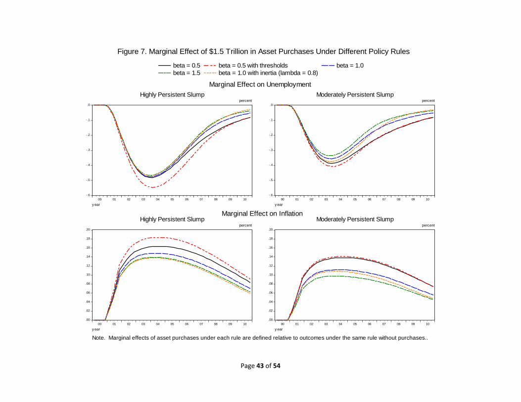
Page 43 of 54  

-.6

-.5

-.4

-.3

-.2

-.1

.0

00 01 02 03 04 05 06 07 08 09 10

beta = 0.5 beta = 0.5 with thresholds beta = 1.0beta = 1.5 beta = 1.0 with inertia (lambda = 0.8)

Highly Persistent Slump

y ear

percent

Marginal Effect on Unemployment

-.6

-.5

-.4

-.3

-.2

-.1

.0

00 01 02 03 04 05 06 07 08 09 10

Moderately Persistent Slump

y ear

percent

.00

.02

.04

.06

.08

.10

.12

.14

.16

.18

.20

00 01 02 03 04 05 06 07 08 09 10

Highly Persistent Slump

y ear

percent

Marginal Effect on Inflation

Note. Marginal effects of asset purchases under each rule are defined relative to outcomes under the same rule without purchases..

.00

.02

.04

.06

.08

.10

.12

.14

.16

.18

.20

00 01 02 03 04 05 06 07 08 09 10

Moderately Persistent Slump

y ear

percent

Figure 7. Marginal Effect of $1.5 Trillion in Asset Purchases Under Different Policy Rules

 

Page 44 of 54  

0.0

0.2

0.4

0.6

0.8

1.0

1.2

1.4

1.6

1.8

2009 2010 2011 2012 2013 2014 2015 2016 2017 2018 2019 2020

Figure 8Evolution of the Perceived Value of Beta Used in Sequential Simulations

(black -- lambda = 0, red -- lambda = .8)

  

Page 45 of 54  

-5

-4

-3

-2

-1

0

1

2

3

4

2008 2010 2012 2014 2016 2018 2020

Real GDP Growth (4-Quarter)percent

4

5

6

7

8

9

10

11

2008 2010 2012 2014 2016 2018 2020

Unemployment Ratepercent

0.8

1.0

1.2

1.4

1.6

1.8

2.0

2.2

2.4

2008 2010 2012 2014 2016 2018 2020

Core PCE Inflation (4-Quarter)percent

0.0

0.5

1.0

1.5

2.0

2.5

3.0

3.5

4.0

2008 2010 2012 2014 2016 2018 2020

no actions (version 1) no actions (version 2) history with Oct-2013 Blue Chip projections

Nominal Federal Funds Ratepercent

Note: The version 1 simulation assumes that agents in the historical baseline always view the fund rate rule as non-inertial. In the version 2 simulations, agentsin the baseline perceive the funds rate rule becoming inertial (lambda=0.8) beginning in 2012.

-2.0

-1.6

-1.2

-0.8

-0.4

0.0

0.4

0.8

1.2

1.6

2008 2010 2012 2014 2016 2018 2020

Real Federal Funds Ratepercent

1.5

2.0

2.5

3.0

3.5

4.0

4.5

5.0

5.5

2008 2010 2012 2014 2016 2018 2020

10-Year Treasury Yieldpercent

Figure 9. Predicted Evolution of the Economy in the Absence of Unconventional Policy

   

Page 46 of 54  

-1.6

-1.4

-1.2

-1.0

-0.8

-0.6

-0.4

-0.2

0.0

0.2

2008 2009 2010 2011 2012 2013 2014 2015 2016 2017 2018

baseline modelrational expectations in financial markets onlyalternative inflation dynamicslow interest elasticity of demandpolicy-linked house price effects

Unemployment Effectspercent

-.1

.0

.1

.2

.3

.4

.5

.6

.7

.8

2008 2009 2010 2011 2012 2013 2014 2015 2016 2017 2018

baseline modelrational expectations in financial markets onlyalternative inflation dynamicslow interest elasticity of demandpolicy-linked house price effects

Inflation Effectspercent

Figure 10. Estimated Effects of of Unconventional Policyin Diferent Specifications of the FRB/US Model

Note. Results expressed as differences from history and the October 2013 Blue Chip forecasts.   

Page 47 of 54 

120

130

140

150

160

170

180

190

200

2008 2009 2010 2011 2012 2013 2014 2015 2016 2017 2018 2019 2020

20092010201120122013

Figure 11. Survey-Based House Price Forecasts

Forecasts beginning in Q1 of years 2010 to 2013 (solid lines) are based on the current and coming year house price projections published in the Q1 Survey of Professional Forecasters; the 2009Q1 forecasts are based on the projections published in the February 2009 Blue Chip survey. Forecasts beginning in Q3 (dashed lines) are based on real-time published data and an average of survey data released in the Q1 SPF for the current and coming years. Beyond the coming year, relative house prices are projected to gradually return to their estimated 1975-2000 trend.

Page 48 of 54  

-6

-4

-2

0

2

4

6

2008 2010 2012 2014 2016 2018 2020

Real GDP Growth (4-Quarter)percent

4

5

6

7

8

9

10

11

2008 2010 2012 2014 2016 2018 2020

Unemployment Ratepercent

0.8

1.0

1.2

1.4

1.6

1.8

2.0

2.2

2.4

2.6

2008 2010 2012 2014 2016 2018 2020

Core PCE Inflation (4-Quarter)percent

0.0

0.5

1.0

1.5

2.0

2.5

3.0

3.5

4.0

2008 2010 2012 2014 2016 2018 2020

version 1 policy (non-inertial) version 2 policy (inertial) history with Oct-2013 Blue Chip projections

Nominal Federal Funds Ratepercent

Note: The version 1 simulation assumes that agents in the historical baseline always view the fund rate rule as non-inertial. In the version 2 simulations, agents in thebaseline perceive the funds rate rule becoming inertial (lambda=0.8) beginning in 2012.

-3

-2

-1

0

1

2

2008 2010 2012 2014 2016 2018 2020

Real Federal Funds Ratepercent

1.0

1.5

2.0

2.5

3.0

3.5

4.0

4.5

5.0

2008 2010 2012 2014 2016 2018 2020

10-Year Treasury Yieldpercent

Figure 12. Predicted Evolution of the Economy if Late-2013 Perceptions of Unconventional PolicyHad Been in Place in Early 2009

 

Page 49 of 54  

Appendix 1 Financial Market Surveys of Policy Expectations and the Economic Outlook 

  Due to data limitations, we cannot directly compared our estimates of the policy expectations of private forecasters implied by the Blue Chip Economic Indicators (BCEI) survey to the beliefs of financial market participants.   However, the forecasts reported in Blue Chip Financial Forecasts (BCFF) and the Federal Reserve Bank of New York’s Primary Dealers Survey (PDS) do allow for some consistency checks.  As shown in Table A1, projections for both the date of liftoff and economic conditions at the time of liftoff are quite similar across the three surveys.  The only major exception occurs in the fall of 2012, when the primary dealers anticipated that liftoff would occur a full year later than the BCEI respondents; this difference may reflect financial market participants’ greater attentiveness to the likelihood of an impending shift in policy at the time.  Table A2 also compares results from the various surveys concerning expected long‐run conditions.  As can be seen, expectations for long‐run rates of inflation and real interest are essentially the same in the BCEI and the BCFF.  Long‐run inflation expectations in the PDS are also similar to those reported in the BCEI; however, the primary dealers reported somewhat higher estimates of the long‐run unemployment rate and the equilibrium real rate.  In addition to these comparisons, Femia, Friedman and Sack (2013) provide another perspective by using the PDS to infer financial market participants’ beliefs about the FOMC’s implicit policy rule.  From early August 2011 through early November 2012, special questions were included in the PDS concerning the likely level of the unemployment rate at the time of liftoff, conditional on different assumptions for the accompanying rate of inflation.  Under some simplifying assumptions, the resulting grid of anticipated unemployment‐inflation combinations can be used to map out changes over time in expectations for the implicit policy reaction function in force at the time of liftoff.  Their analysis suggests that market expectations in August 2011 were consistent with a simple policy rule in which β equals 1.0 but that the perceived value of this coefficient had risen to 1.25 by September 2012, conditional on α equaling 0.5.45  Both values are somewhat higher that the corresponding BCEI estimates reported in Table 4.   

 

 

                                                            45 The estimated value of β is somewhat sensitive to how movements in the unemployment rate are translated into movements in the output gap—that is, into the value of Okun’s Law coefficient.  Consistent with assumptions made elsewhere in this paper, we have assumed that this coefficient equals 2.0; if we had instead set Okun’s Law coefficient to 2.3, as Femia, Friedman and Sack did in their study, the implied value of β would fall to 0.9.  In addition, the value of β implied by the PDS results depends linearly on the assumed value of α.  By themselves, the survey questions cannot be used to estimate the perceived values of both α and β unless one is willing to make assumptions regarding market beliefs concerning R*, π*, the natural rate of unemployment, and Okun’s Law.  Reasonable variations in assumptions for these factors yield estimates of α that range from 0.25 to 1.00, with higher values of α implying higher estimated values of β. 

Page 50 of 54  

Table A1 Comparison of Blue Chip Projections of Liftoff Conditions with Corresponding Forecasts from Financial Market Participants 

 

 Projected Liftoff Date for the Federal 

Funds Rate  

Q4 Unemployment Rate in Projected Liftoff Year 

 Annual GDP or Core PCE Inflation Rate 

in Projected Liftoff Year 

  Blue Chip Blue Chip Financial Forecasts 

Primary Dealers Survey 

  Blue Chip Primary Dealers Survey 

 Blue Chip 

(GDP) 

Blue Chip Financial Forecasts 

(GDP) 

Primary Dealers Survey 

(core PCE) 

Survey release date                     

    March 2009  2009Q4  2010Q1      9.2      1.0  1.6   

    October 2009  2010Q3  2010Q2      9.6      1.4  1.5   

    March 2010  2010Q4  2010Q3      9.6      1.4  1.2   

    October 2010  2011Q4  2011Q3      9.1      1.4  1.5   

    March 2011  2012Q1  2011Q4  2012Q3    8.1  7.9    1.6  1.9  1.6 

    October 2011  2013Q31  Mid‐2013  2013Q4    8.11  8.3    2.0  2.1  1.6 

    March 2012  2014Q11  2014Q12  2014Q3    7.01  7.0    2.1  2.1  2.0 

    October 2012  2014Q31    2015Q3    7.11  7.0    2.0    1.9 

    March 2013  2015Q21  2015H23  2015Q3    6.51  6.5    2.1  2.1  2.0 

    October 2013  2015Q21  2015H23  2015Q3    6.31  6.1    2.1  2.0  1.9 

Note.  For October releases, Primary Dealer Survey results reflect the survey taken in mid‐September. 1. Imputed using quarterly and annual forecast data. 2. Date inferred from respondents’ assessment that there was a 69% probability of liftoff occurring in 2014Q1 or later, and a 31% probability that it would occur earlier. 3. Most likely date based on respondents reported probability assessments. 

 

   

Page 51 of 54  

 Table A2 

Comparison of Blue Chip Projections of Long‐Run Conditions with Corresponding Forecasts from Financial Market Participants  

  Long‐Run Real Federal Funds Rate1   Long‐Run 

Unemployment Rate   Long‐Run GDP Inflation Rate2 

  Blue Chip Blue Chip Financial Forecasts3 

Primary Dealers Survey4 

  Blue Chip Primary Dealers Survey4 

  Blue Chip 

Blue Chip Financial Forecasts3 

Primary Dealers Survey4 

Blue Chip Survey Release Date                   

    March 2009  2.0  1.8      5.5      2.3  2.4   

    October 2009  2.2  1.9      5.8      2.1  2.3   

    March 2010  2.1  1.9      6.0      2.2  2.2   

    October 2010  1.9  1.8      5.9      2.1  2.1   

    March 2011  1.9  1.6      5.6      2.1  2.2   

    October 2011  1.7  1.6      6.0      2.1  2.1   1 6    March 2012  1.6  1.5      5.8  6.2    2.2  2.1  2.1 

    October 2012  1.6  1.6  1.9    5.8  6.0    2.1  2.2  2.1 

    March 2013  1.6  1.6  1.9    5.6  6.0    2.1  2.2  2.1 

    October 2013  1.6  1.6  1.9    5.6  5.9    2.1  2.1  2.1 

1. For the Blue Chip survey, federal funds rate forecasts are approximated by the projected Treasury bill rate plus 10 basis points.  For all three surveys, real rates are constructed by subtracting the long‐run projection for GDP price inflation.      

2. The Primary Dealers Survey only reports inflation forecasts on a PCE or a CPI basis, so inflation forecasts on a GDP basis are constructed from PCE‐based measures by adding 10 basis points, and from CPI‐based measures by subtracting 20 basis points.   

3. Blue Chip Financial Forecasts only report extended forecasts in June and December, so results from these two months are used for March and December, respectively. 4. October results for the Primary Dealers Survey are based on surveys taken in mid‐September immediately prior to the FOMC meeting. 

 

 

Page 52 of 54  

Appendix 2 Financial Market Responses to QE Events: A Summary of Event Study Results 

 

In this Appendix, we summarize the findings of a number of recent studies that examine the responses 

of various yields and asset prices to the announcement of large‐scale asset purchases.  This evidence, 

which mostly relies on event studies, is important because it presents the first step in the transmission 

of QE policies to real activity and inflation, and because it provides evidence against which to assess the 

transmission mechanism of a model used to evaluate the macroeconomic effects of these policies.46 

Mortgage rates.  Hancock and Passmore (2014) estimate substantial effects of LSAPs on the secondary‐

market yields on agency MBS and only slightly smaller effects on primary‐market conforming home 

mortgage rates.  Moreover, they report evidence that the Federal Reserve’s purchases of agency MBS 

have an extra effect on the yields on those securities (relative to Treasury yields) and that, over time, a 

large portion of those effects also pass through to primary mortgage rates.47  For example, following the 

announcement of the new asset purchase program in September 2012, the spread between agency MBS 

yields and 10‐year Treasury yields fell noticeably after both the initial announcement of and subsequent 

communications about this program.  Moreover, although the spread between the interest rates on 

conforming 30‐year fixed‐rate loans and agency MBS yields widened at first, this spread gradually 

moved back down to below its late‐August 2012 level, which is consistent with essentially all of the 

decrease in agency MBS yields brought about by the additional purchases eventually passing through to 

conforming mortgage interest rates.   

Corporate yields.  Recent research has also reported substantial pass‐through of LSAP‐induced changes 

in Treasury yields to yields on investment‐grade corporate bonds.  Gilchrist, López‐Salido, and Zakrajšek 

(2014) find almost complete pass‐through of LSAP‐induced reductions in Treasury yields to yields on 

investment‐grade corporate bonds, while Kiley (2013a) estimates that about three‐quarters of the drop 

in Treasury yields passed through.  By contrast, pass‐through of LSAP effects to yields on speculative‐

grade corporate bonds has been found to be small (except in some analyses of the first round of LSAPs, 

which was announced at a time when markets were highly dysfunctional and risk spreads exceptionally 

wide).  For example, focusing on the Federal Reserve’s balance sheet actions from late‐2008 through 

2010, Krishnamurthy and Vissing‐Jorgenson (2011) reported essentially complete pass‐through of lower 

long‐term Treasury yields to investment‐grade corporate bond yields from the first two LSAPs, but 

sizable pass‐through to speculative‐grade corporate bond yields only for the first round of LSAPs in the 

winter of 2008 and 2009. 

Exchange rate.  Glick and Leduc (2013) document that LSAP announcements scaled to a 20 basis point 

reduction in 10‐year Treasury yields have tended to lower the broad currency index used in FRB/US by 

about ¾ percent.  Kiley’s (2013b) econometric analysis of selected bilateral exchange rates implies that a 

20 basis point reduction in the 10‐year Treasury yield over the period since nonconventional policies 

                                                            46 We thank Michael Palumbo for helpful advice on this appendix. 47 In this and an earlier paper (Hancock and Passmore, 2012), the authors emphasized that the extent of pass‐through of changes in agency MBS yields to primary mortgage rates appears to depend on prevailing market conditions, including the level of mortgage rates:  Pass‐through has tended to be more complete when mortgage rates are higher than lower, likely reflecting in part the effects of limited capacity in the mortgage origination industry. 

Page 53 of 54  

have been undertaken led to a 1½ to 2 percent depreciation of the dollar against the euro and the 

Japanese yen.  

Equity prices.  Turning to the stock market reactions to news about the Federal Reserve’s balance sheet 

policies, event study of stock market responses in narrow windows around FOMC announcements and 

other communications associated with the first two rounds of LSAPs suggested a response of close to 2 

percent for a 20 basis point decrease in the 10‐year Treasury yield.  Rosa (2012) and Kiley (2013c) 

estimated the stock market effects of changes in Treasury term premiums induced by LSAPs (holding 

market expectations for path of the federal funds rate roughly constant) and found smaller responses—

averaging about a 1 percent increase in stock prices for an LSAP‐induced 20 basis point decrease in the 

10‐year Treasury term premium. 

Summary.  There are reasons to think that the stock market response to LSAPs could depend 

importantly on prevailing market conditions and that event studies might not always pick up the full 

effect of such monetary policy actions.  The first LSAPs—announced in late‐2008 and early 2009—

appear to have been key elements in a suite of policy responses to the financial crisis that significantly 

bolstered equity prices over time.48  Estimates of the equity premium had soared during the most acute 

phase of the financial crisis that autumn, but narrowed substantially in the spring and summer of 2009, 

as U.S. stock prices climbed.  A similar but less pronounced pattern was evident around the time of 

LSAP‐related news and announcements in the summer of 2010.  These observations suggest that a 

considerable part of the stock market response to the first two rounds of LSAPs occurred outside of 

narrow event windows.  

In addition, the evidence indicates that the earlier rounds of LSAPs led market participants to expect a 

more accommodative stance of conventional monetary policy (Bauer and Rudebusch, 2012, and 

Krishnamurthy and Vissing‐Jorgenson, 2011), which could have produced a relatively strong 

transmission since conventional monetary policy actions have been shown to generate sizable stock 

market responses (Bernanke and Kuttner, 2005, Rosa, 2012, Kiley, 2013c).  Because the FOMC was 

already using calendar‐based guidance regarding the likely medium‐term path of federal funds rate in 

September 2012 and shifted to quantitative thresholds for its forward guidance in December 2012, the 

scope for LSAP announcements to operate forcefully through such a signaling channel may have been 

limited at the time of the announcement of LSAP3. 

In sum, these event studies suggest that the first two rounds of LSAPs probably spurred larger responses 

of interest rates, the exchange value of the dollar, and equity prices than later ones because the earlier 

programs were announced and implemented at times when market conditions were highly strained and 

risk premiums were exceptionally large or when there was greater scope for signaling more 

accommodative intentions with respect to the federal funds rate.  The following table reports the 

central tendency of estimates of the effects of a hypothetical LSAP program, scaled to an initial impact 

on 10‐year Treasury yields of ‐20 basis points, on selected financial market quotes; of course, there is a 

great deal of uncertainty surrounding all these figures. 

  

                                                            48 For example, the completion of the Federal Reserve’s Supervisory Capital Assessment Program for the major banking firms also appeared to play an important role in allaying some of the concerns among market participants. 

Page 54 of 54  

Table 1 Effects of a Hypothetical LSAP Program on Selected Financial Market Quotes 

 

10‐year Treasury yield  −20 basis points 30‐year current coupon agency MBS yield  −27 basis points Conforming 30‐year (fixed) mortgage rate  −25 basis points BBB corporate bond yield  −15 basis points Exchange value of the dollar (broad index)  −3/4 percent S&P 500 stock price index  1‐3/4 percent 

 

Note. This hypothetical program is assumed to involve purchases of equal amounts of longer‐term Treasury 

securities and agency MBS.