NBER WORKING PAPER SERIES

THE ORIGINS AND EFFECTS OF MACROECONOMIC UNCERTAINTY

Francesco BianchiHoward Kung

Mikhail Tirskikh

Working Paper 25386http://www.nber.org/papers/w25386

NATIONAL BUREAU OF ECONOMIC RESEARCH1050 Massachusetts Avenue

Cambridge, MA 02138December 2018

We thank Nick Bloom, Jesus Fernandez-Villaverde, Francisco Gomes, Francois Gourio, Giorgio Primiceri, Hikaru Saijo, and all seminar participants at 2017 SITE Summer workshop on uncertainty, NBER, Duke University, ESOBE conference, IAAE conference, and London Business School for helpful comments and suggestions. An earlier version of this paper circulated with the title “Pricing Macroeconomic Uncertainty.” The views expressed herein are those of the authors and do not necessarily reflect the views of the National Bureau of Economic Research.

NBER working papers are circulated for discussion and comment purposes. They have not been peer-reviewed or been subject to the review by the NBER Board of Directors that accompanies official NBER publications.

© 2018 by Francesco Bianchi, Howard Kung, and Mikhail Tirskikh. All rights reserved. Short sections of text, not to exceed two paragraphs, may be quoted without explicit permission provided that full credit, including © notice, is given to the source.

The Origins and Effects of Macroeconomic UncertaintyFrancesco Bianchi, Howard Kung, and Mikhail TirskikhNBER Working Paper No. 25386December 2018JEL No. C11,C32,E32,G12

ABSTRACT

We construct and estimate a dynamic stochastic general equilibrium model that features demand- and supply-side uncertainty. Using term structure and macroeconomic data, we find sizable effects of uncertainty on risk premia and business cycle fluctuations. Both demand-side and supply-side uncertainty imply large contractions in real activity and an increase in term premia, but supply-side uncertainty has larger effects on inflation and investment. We introduce a novel analytical decomposition to illustrate how multiple distinct risk propagation channels account for these differences. Supply and demand uncertainty are strongly correlated in the beginning of our sample, but decouple in the aftermath of the Great Recession.

Francesco BianchiSocial Sciences Building, 201BDepartment of EconomicsDuke UniversityBox 90097Durham, NC 27708-0097and CEPRand also NBERfrancesco.bianchi@duke.edu

Howard KungLondon Business SchoolRegent's Park, Sussex PlaceLondon NW1 4SAUnited Kingdomhkung@london.edu

Mikhail TirskikhLondon Business Schoolmtirskikh@london.edu

1 Introduction

It is well-established that broad measures of macroeconomic and financial market uncertainty vary signifi-

cantly over time.1 There is also an emerging literature interested in studying how these changes in uncertainty

affect business cycle fluctuations in micro-founded general equilibrium models. With a few exceptions, this

literature tends to find that uncertainty is not among the main sources of macroeconomic fluctuations.

However, these papers typically only use macroeconomic data to pin down the effects of uncertainty, con-

sider only one source of uncertainty, and rely on calibration exercises in which the process for uncertainty

is separately estimated.2 In this paper, we use both macroeconomic and term structure data, distinguish

between demand-side and supply-side uncertainty, and conduct a structural estimation of a micro-founded

model in which the process for uncertainty and its effects are jointly estimated. Our results demonstrate

that uncertainty matters. In particular, we uncover sizable effects of uncertainty shocks on business cycle

and term premia dynamics. The specific effects of demand-side and supply-side uncertainty are examined

through multiple endogenous risk propagation channels.

Asset prices contain valuable information about uncertainty, given that changes in macroeconomic un-

certainty generate fluctuations in risk premia. We find that changes in nominal term premia contain key

identifying information disciplining the effects of uncertainty and its propagation through various risk chan-

nels. At the same time, there is empirical and anecdotal evidence suggesting that changes in measures of

uncertainty are related to heterogeneous sources (e.g., Bloom (2014)) and are also imperfectly correlated.

Figure 1 plots various uncertainty measures whose pairwise correlations range between -0.30 to 0.85. We

find it important to distinguish between different sources of uncertainty, and we explicitly model fluctuating

demand and supply uncertainty. We identify demand uncertainty as originating from shocks to the time

discount factor while supply uncertainty as emanating from shocks to TFP growth. In particular, we show

that these two types of uncertainty act through distinct channels. Finally, jointly estimating the process

for uncertainty and its effects on the economy has the important implication that uncertainty is not only

identified via changes in stochastic volatility, but also through its first-order effects on the economy.

Our quantitative analysis is based on a dynamic stochastic general equilibrium (DSGE) model along the

lines of Christiano, Eichenbaum, and Evans (2005), but with the following departures. First, we assume that

the representative household has Epstein and Zin (1989) recursive preferences to capture sensitivity towards

low-frequency consumption growth and discount rate risks. Second, we allow for stochastic volatility changes

1See, for example, Baker, Bloom, and Davis (2016) and Jurado, Ludvigson, and Ng (2015)2Some examples include Bloom (2009), Bloom, Floetotto, Jaimovich, Saporta-Eksten, and Terry (2012), and Basu

and Bundick (2017).

1

in TFP and preference shocks, both modeled as distinct Markov chains, estimated jointly within our DSGE

model. Changes in stochastic volatility and the endogenous response of the economy to these changes

both contribute to fluctuations in uncertainty. Third, we use an iterative solution method to endogenously

capture sizable and time-varying risk premia. By modelling stochastic volatility as regime changes, we obtain

a conditionally log-linear solution that facilitates an estimation using a modification of the standard Kalman

filter. Lastly, we use data on nominal bond yields across different maturities in our estimation.

Our solution method captures the first- and second-order effects of uncertainty on agents’ decision poli-

cies, as well as effects on conditional risk premia. We show that this feature of our solution method sharpens

the identification of uncertainty dynamics. In addition, our solution method provides an approximate an-

alytical risk decomposition that uncovers distinct risk propagation channels for which uncertainty affects

macroeconomic fluctuations. We use the risk decomposition to illustrate how uncertainty shocks produce

different effects depending on the origin (e.g., demand or supply). Our analysis therefore provides an eco-

nomic interpretation for why there is not a consensus on the macroeconomic effects of uncertainty shocks.

More broadly, our risk decomposition can be utilized in a wide range of dynamic stochastic models, and is

therefore of independent interest.

Figure 2 illustrates the strong relation between real activity, measured as detrended GDP, the slope of the

nominal yield curve, and macroeconomic volatility.3 As the economy enters a recession, the slope of the yield

curve and macroeconomic volatility both tend to rise. In our model, movements from low to high volatility

regimes endogenously trigger a decline in real activity and a steepening of the yield curve, consistent with

the data. We find that the effects of uncertainty are quantitatively significant. The two uncertainty shocks

together explain over 14% of the variation in investment growth, around 10% for consumption growth, and

28% for the slope of the nominal yield curve. These shocks also produce significant countercyclical variation

in the nominal term premium. The effects of uncertainty are even more sizable when focusing on fluctuations

at business cycle frequencies. An economy that is exclusively affected by uncertainty shocks would generate

business cycle fluctuations for consumption and investment as large as 24.5% and 31%, respectively, of an

analogue economy with both uncertainty and traditional level shocks.

Both demand-side and supply-side uncertainty generate positive commovement between consumption and

investment, which is often a challenge for standard macroeconomic models. Thus, uncertainty shocks emerge

as an important source of business cycle fluctuations. However, the origin of uncertainty plays an important

role, as the two types of uncertainty impact the economy in very distinct ways. Compared to demand-

3Detrended GDP is obtained by applying a bandpass filter. Similar results hold if GDP is detrended using an HPfilter. The slope of the term structure is computed as the difference between the five-year yields and the one-yearyield. Macroeconomic volatility is measured as a five-year moving average of the standard deviation of GDP growth.

2

side uncertainty, supply-side uncertainty has larger effects on inflation and is relatively more important

for explaining fluctuations in investment. Furthermore, while in the first half of our sample, demand- and

supply-side uncertainty tend to move together, they decouple in the second half of the sample.

Nominal term premia in our model is driven by time-varying demand and supply uncertainty. As such,

using the term structure of interest rates as observables in our estimation is important for disciplining the

effects of uncertainty. While both supply and demand uncertainty are important for the unconditional nom-

inal term premia, we find that the conditional dynamics of nominal term premia are mostly attributed to

variation in demand-side uncertainty through the inflation risk premia component. Therefore, the observed

term structure dynamics help to sharpen the identification of the two different sources of uncertainty. With-

out using term structure data in our estimation, the timing of the uncertainty shocks is quite different, the

volatility regimes are less persistent, and the effects of the uncertainty shocks on the macroeconomy are

smaller.

To understand how uncertainty shocks affect the real economy and account for these differences, we use

an approximate model solution method that allows us to identify and quantify five distinct risk propagation

channels for uncertainty shocks that are labeled as precautionary savings, investment risk premium, inflation

risk premium, nominal pricing bias, and investment adjustment channel. The precautionary savings term

reflects the prudence of the representative household towards uncertainty about future income. This prudence

term arises through the households’ consumption-savings Euler equation. The investment risk premium term

emerges through the investment Euler equation, which depends on the covariance between the pricing kernel

and the return on investment. The inflation risk premium term shows up through the Fisherian equation,

and the nominal term premium imposes strong restrictions on this channel. The nominal pricing bias

arises in the Phillips curve due to the presence of nominal rigidities that makes firms more prudent when

setting nominal goods prices. Finally, the investment adjustment channel arises because of rigidities in the

household’s ability to immediately adjust investment to the desired level.

Our decomposition of the risk propagation channels show that different forces contribute to generating

empirically realistic macroeconomic and asset pricing dynamics. The precautionary savings, investment risk

premium, and the nominal pricing bias terms are the most quantitatively important risk propagation channels

for business cycles. The parameters governing price stickiness, capital adjustment costs, and elasticity of

labor supply are critical for determining the effects from these risk propagation channels. Price stickiness

and labor supply elasticity are important for determining the sign and magnitude of the precautionary

savings channel, while capital adjustment costs are important for determining the sign and magnitude of the

investment risk premium channel. The degree of price stickiness and labor supply elasticity determines the

3

sensitivity of labor demand shifts to uncertainty changes. The degree of capital adjustment costs affects the

covariance of the return on investment and the stochastic discount factor, which determines the effect of the

investment risk premium channel. The degree of price stickiness is important for determining the effects of

the nominal pricing bias.

The investment risk premium channel plays a key role in amplifying the response of investment to changes

in supply-driven uncertainty. The investment risk premium channel has opposite effects on investment for

supply- and demand-side uncertainty. The underlying reason is that physical capital is a poor hedge against

negative TFP shocks, but a good hedge for adverse preference shocks. In particular, demand and supply-side

shocks produce different signs in the covariance between the pricing kernel and the return on investment.

In response to a negative TFP shock, marginal utility increases but the value of physical capital decreases.

Therefore, investment in physical capital commands a positive risk premium with respect to TFP shocks.

In contrast, preference shocks produce the opposite pattern. A negative preference shock increases marginal

utility and the value of capital. Therefore, investment commands a negative risk premium with respect to

preference shocks. Consequently, when supply-side uncertainty increases, households have an incentive to

lower investment so as to reduce exposure to TFP shocks. Instead, when demand-side uncertainty increases,

households have an incentive to increase investment to hedge against preference shocks. Overall, this channel

plays a key role in explaining why the cumulative decline in investment to an increase supply-side (demand-

side) uncertainty is amplified (dampened).

We then use our decomposition to understand the small response of inflation to demand-driven uncer-

tainty shocks, but a large response to supply-driven uncertainty. These inflation responses can be accounted

for by differences in how the precautionary savings and nominal pricing bias channels operate under the two

uncertainty shocks. Both demand- and supply-side uncertainty shocks trigger a strong precautionary savings

channel effect, which generates downward pressure on inflation. However, for demand-driven uncertainty,

another quantitatively important propagation channel is the nominal pricing bias, which is natural given

that level preference shocks are one of the main drivers of inflation dynamics. For demand-side uncertainty

shocks, the precautionary savings and nominal pricing bias channels have opposite effects on inflation that

cancel each other out, and consequently, the cumulative effect on inflation is close to zero. In contrast,

for supply-side uncertainty, the nominal pricing bias is not quantitatively important, since TFP growth

shocks are not important for explaining inflation dynamics. Therefore, the cumulative effect of an increase

in supply-side uncertainty is driven by the precautionary savings propagation channel, leading to a large

decline in inflation.

Our paper relates to Basu and Bundick (2017) in that we also consider the role of the precautionary

4

savings channel, in conjunction with sticky prices, for the propagation of demand-side uncertainty shocks.

In our estimation, we find that this channel is quantitatively important. Thus, we complement the findings

of Basu and Bundick (2017), but differ along the following dimensions. First, we develop a novel analyt-

ical decomposition that unveils four additional risk propagation channels. In our estimation, we find that

two of these four channels, the investment risk premium and nominal pricing bias, are as quantitatively

important as the precautionary savings channel. Second, we conduct a structural estimation of our model

using macroeconomic and bond yield data instead of calibration. In our structural estimation the process

for uncertainty is not exogenously given, but jointly estimated with the rest of the model. We find that un-

certainty plays a key role for both macro and term structure dynamics. Finally, we allow for both demand-

and supply-side uncertainty changes, while Basu and Bundick (2017) only consider demand-side uncertainty

shocks. While both types of uncertainty shocks are important for explaining business cycles, we find that

the macroeconomic responses to these shocks to be quite different. For example, supply-side uncertainty

changes generate more severe recessions, with significantly larger effects on inflation and investment. Our

analytical decomposition allows us to carefully disentangle the economic margins that account for these

different responses.

Our paper connects to the broader literature studying the impact of uncertainty shocks in macroe-

conomic models (e.g., Bloom (2009), Bloom, Floetotto, Jaimovich, Saporta-Eksten, and Terry (2012),

Bachmann and Bayer (2014), Fernandez-Villaverde, Guerron-Quintana, Rubio-Ramırez, and Uribe (2011),

Fernandez-Villaverde, Guerron-Quintana, Kuester, and Rubio-Ramırez (2015), Justiniano and Primiceri

(2008), Bianchi, Ilut, and Schneider (2014), Schaal (2017), Fajgelbaum, Schaal, and Taschereau-Dumouchel

(2017), and Saijo (2017), etc.). We differ from these papers in that we (i) allow for multiple sources of

uncertainty, (ii) conduct a structural estimation, (iii) use asset pricing data, in the form of nominal bond

yields in the estimation and a prior on the investment risk premium, to discipline the effects of uncertainty,

and (iv) do not deviate from the assumption of rational expectations.

The pricing of consumption and volatility risks builds on the endowment economy models of Bansal and

Yaron (2004), Piazzesi and Schneider (2007), and Bansal and Shaliastovich (2013). However, we differ by

considering a general equilibrium framework with production, where the dynamics of stochastic consumption

volatility risks are linked to the time-varying second moments of structural macroeconomic shocks and to

the endogenous response of the macroeconomy to changes in the volatility of these shocks. Furthermore, our

production-based setting allows us to consider the endogenous feedback between risk premia and business

cycle fluctuations via uncertainty shocks. The role of preference shocks for generating a positive real term

premia relates to the endowment economy model of Albuquerque, Eichenbaum, Luo, and Rebelo (2016). We

5

build on this work, and show that time discount factor shocks also provide a novel endogenous source of

inflation risk premia in a New Keynesian framework.

More broadly, our paper relates to an emerging literature studying asset prices in New Keynesian mod-

els (e.g., Bekaert, Cho, and Moreno (2010), Bikbov and Chernov (2010), Hsu, Li, and Palomino (2014),

Rudebusch and Swanson (2012), Dew-Becker (2014), Bretscher, Hsu, and Tamoni (2017), Weber (2015),

Kung (2015), and Campbell, Pflueger, and Viceira (2014)). With respect to these papers, we conduct a

structural estimation of a micro-founded model assuming continuity between how assets are priced by the

representative agent in the model and by the econometrician.

This paper is organized as follows. Section 2 presents a simplified model to introduce the decomposition

of the effects of uncertainty into five distinct risk channels. In this section, we also explain our solution

approach. Section 3 describes the full model. Section 4 contains the main results. Section 5 concludes.

2 Risk Propagation Channels

To illustrate the key model mechanisms and our solution method, we consider a simplified version of the

benchmark model used for structural estimation. We find that in a New-Keynesian model, uncertainty shocks

can be contractionary – even when the precautionary savings channel places upward pressure on investment

– due to the presence of four other risk propagation channels, unveiled in our analytical decomposition char-

acterized below. Thus, the overall effect of uncertainty is determined by how uncertainty propagates through

the different channels. Analyzing uncertainty changes through the lens of these risk propagation channels

helps us to understand (i) the heterogeneous effects of different uncertainty shocks on the macroeconomy,

(ii) the role of risk premia for imposing restrictions on the propagation channels, and (iii) how various model

frictions pin down the effect of the propagation channels. This approach can be applied to other models and

it is therefore of independent interest.

2.1 Simplified Model

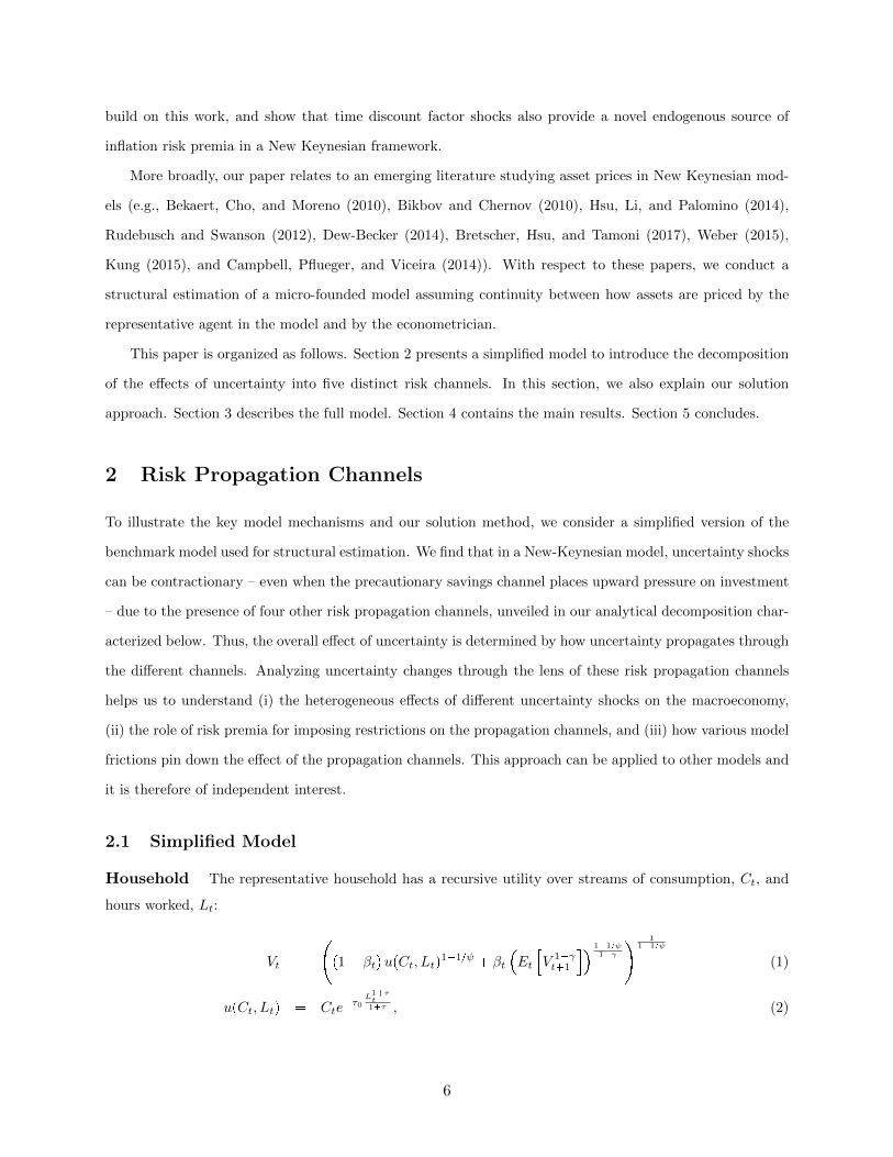
Household The representative household has a recursive utility over streams of consumption, Ct, and

hours worked, Lt:

Vt �

�p1 � βtqupCt, Ltq

1�1{ψ � βt

�Et

�V 1�γt�1

� 1�1{ψ1�γ

� 11�1{ψ

(1)

upCt, Ltq � Cte�τ0

L1�τt

1�τ , (2)

6

where γ is the coefficient of risk aversion, ψ is the elasticity of intertemporal substitution. The household

also supplies labor services, Lt, to a competitive labor market at a real wage Wt. In the limit, when ψ Ñ 1,

the preferences specified above become

Vt � upCt, Ltqp1�βtq

�Et

�V 1�γt�1

� βt1�γ

(3)

This is the case that we consider below.

We define a preference shock, bt, such that, βt �1

1�βebt. The preference shock, bt, follows an AR(1)

process, with volatility of innovations depending on the aggregate volatility regime, ξt:

bt�1 � ρβ bt � σβ,ξt�1εβ,t�1. (4)

The volatility regime, ξt, follows a Markov-switching process with a transition matrix H.

The representative household owns capital, Kt�1, pre-determined at time t � 1, which it supplies to

competitive capital markets at a real rental rate rkt . The household accumulates capital according to the

following law of motion:

Kt � Kt�1 p1 � δ0q � r1 � S pIt{It�1qs It (5)

S pIt{It�1q � pϕI{2q pIt{It�1 � eµq2, (6)

where It is time t investment and the function S pIt{It�1q reflects capital adjustment costs.

The time t budget constraint of the household is

PtCt � PtIt �Bt�1{Rt � PtDt � PtWtLt �Bt � PtKt�1rkt (7)

where Pt is the nominal price of the consumption good, Bt�1 is the amount of nominal one-period bonds

held by household at time t with maturity at time t� 1, Rt is the gross nominal interest rate set at time t

by the monetary authority, Dt is the real dividend income received from the intermediate firms

The optimization problem of the household results in the following intertemporal first order condition:

1 � Et rMt�1Pt{Pt�1sRt, (8)

where

Mt�1 �1 � βt�1

1 � βtβt

�� V 1�γt�1

Et

�V 1�γt�1

�� �

Ct�1

Ct

�1

(9)

7

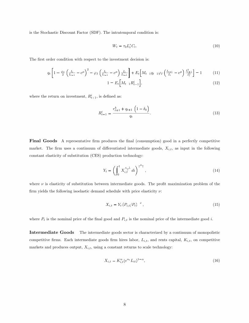
is the Stochastic Discount Factor (SDF). The intratemporal condition is:

Wt � τ0LτtCt. (10)

The first order condition with respect to the investment decision is:

qt

�1 � ϕI

2

�ItIt�1

� eµ2

� ϕI

�ItIt�1

� eµ

ItIt�1

�� Et

�Mt�1qt�1ϕI

�It�1

It� eµ

I2t�1

I2t

�� 1 (11)

1 � Et

�Mt�1R

it�1

�, (12)

where the return on investment, Rit�1, is defined as:

Rit�1 �rkt�1 � qt�1

�1 � δ0

qt

. (13)

Final Goods A representative firm produces the final (consumption) good in a perfectly competitive

market. The firm uses a continuum of differentiated intermediate goods, Xi,t, as input in the following

constant elasticity of substitution (CES) production technology:

Yt �

�» 1

0

Xν�1ν

i,t di

νν�1

, (14)

where ν is elasticity of substitution between intermediate goods. The profit maximization problem of the

firm yields the following isoelastic demand schedule with price elasticity ν:

Xi,t � Yt pPi,t{Ptq�ν, (15)

where Pt is the nominal price of the final good and Pi,t is the nominal price of the intermediate good i.

Intermediate Goods The intermediate goods sector is characterized by a continuum of monopolistic

competitive firms. Each intermediate goods firm hires labor, Li,t, and rents capital, Ki,t, on competitive

markets and produces output, Xi,t, using a constant returns to scale technology:

Xi,t � Kαi,tpe

ntLitq1�α, (16)

8

where nt is a stochastic productivity trend with the following law of motion:

∆nt � µ� xt, (17)

xt � ρxxt�1 � σx,ξtεx,t, εx,t � N p0, 1q , (18)

where µ is the unconditional mean of productivity growth and xt is a TFP growth shock. Note that the

standard deviation σx,ξt depends on the volatility regime ξt.

The intermediate firms face a cost of adjusting the nominal price a la Rotemberg (1982), measured in

terms of the final goods as

GpPi,t, Pi,t�1, Ytq �φR2

�Pi,t

ΠssPi,t�1� 1

2

Yt, (19)

where Πss ¥ 1 is the steady-state inflation rate and φR is the magnitude of the price adjustment costs. The

source of funds constraint is :

PtDi,t � Pi,tXi,t � PtWtLi,t � PtrktKi,t � PtGpPi,t, Pi,t�1, Ytq, (20)

where Di,t is the real dividend paid by the firm. The objective of the firm is to maximize shareholder’s value,

Vpiqt � V piqp�q, taking the pricing kernel, Mt, the competitive real wage, Wt, the real rental rate of capital,

rkt , and the vector of aggregate state variables Ψt � pPt, Zt, Ytq as given:

V piq pPi,t�1;Ψtq � maxPi,t,Li,t,Ki,t

!Di,t � Et

�Mt�1 V

piq pPi,t;Ψt�1q�), (21)

subject to

Di,t �Pi,tPt

Xi,t �WtLi,t � rktKi,t �GpPi,t, Pi,t�1, Yt, q (22)

Xi,t � Yt

�Pi,tPt

�ν

, (23)

Xi,t � Kαi,tpZtLi,tq

1�α. (24)

The optimization problem results in the first-order condition corresponding to the price setting decision:

p1 � νq�Pi,tPt

�νYtPt� νWt

Li,t1�α

�Pi,tPt

�11Pt

�φR

�Pi,t

ΠssPi,t�1� 1

Yt

ΠssPi,t�1� Et

�Mt�1φR

�Pi,t�1

ΠssPi,t� 1

Yt�1Pi,t�1

ΠssP 2i,t

�� 0, (25)

and the first-order condition for the amount of capital:

rkt �α

1 � αWt

Li,tKi,t

. (26)

9

Central Bank The central bank follows a Taylor rule that depends on output and inflation deviations

from steady-state:

ln

�RtRss

� ρr ln

�Rt�1

Rss

� p1 � ρrq

�ρπ ln

�Πt

Πss

� ρy ln

� pYtpYss�

� σR,ξtεR,t, (27)

where Rt is the gross nominal short rate, Πt � Pt{Pt�1 is the gross inflation rate, pYt � Yt{Zt is detrended

output, and εR,t � N p0, 1q is a monetary policy shock. Variables with a ss subscript denote steady-state

values.

Symmetric Equilibrium In the symmetric equilibrium, all intermediate firms make identical decisions:

Pi,t � Pt, Xi,t � Xt � Yt, Ki,t � Kt, Li,t � Lt, Di,t � Dt. Also, nominal bonds are in zero net supply

Bt � 0. Clearing of capital market implies Ki,t � Kt�1. The aggregate resource constraint is

Yt � Ct � It � .5φR pΠt{Πss � 1q2Yt. (28)

2.2 Log-linearization with risk-adjustment

Our goal is to study the effects of uncertainty on both asset prices and the macroeconomy. If standard log-

linearization techniques were applied, all of the effects of uncertainty would be lost. Instead, we implement a

risk-adjusted log-linearization of the model (e.g., Jermann (1998), Lettau (2003), Backus, Routledge, and Zin

(2010), Uhlig (2010), Dew-Becker (2012), Malkhozov (2014), and Bianchi, Ilut, and Schneider (2014)). The

idea behind this approximation method is that all expectational equations are approximated assuming that

the variables are conditionally log-normal. The approximate solution indeed satisfies this condition, because

it is linear in the state variables. Then we solve a resulting system of linear expectational difference equations

augmented with an iterative procedure designed to capture a risk-adjustment component. This procedure

allows us to solve rational expectation models in which uncertainty is controlled by a Markov-switching

process by using solution methods that have been developed for log-linear approximations. It is important

to emphasize that we allow risk to affect not only asset prices, but also the policy functions controlling the

macroeconomic variables. This is crucial to study the effects of uncertainty on the macroeconomy.

We apply the risk adjusted log-linearization to the first-order conditions and market clearing conditions

presented above. Define the risk-free rate, Rf,t as the return on a theoretical risk-free asset, which pays one

10

unit of consumption good in every state of the world next period. The risk-free rate satisfies the following

asset pricing equation:

1 � Et

�Mt�1Rf,t

�, (29)

or1

Rf,t� Et

�Mt�1

�(30)

As described above, the log-linearization approach that we are using approximates all expectational equations

assuming that the variables are conditionally log-normal. So, log-linearizing (30), we get

�rrf,t � Et

� rmt�1

��

1

2V art

� rmt�1

�(31)

Here, and below, variables with a tilde denote log-deviations from the deterministic steady state of the

corresponding variables.4 We can then log-linearize the expression for the stochastic discount factor (9)

using our risk adjustment approach:5

rmt�1 �

�� βrbt�1 �rbt � p1 � γqprvt�1 � Etrrvt�1 � rxt�1sq � prct�1 � rctq�γrxt�1 �

12 p1 � γq2V artrrvt�1 � rxt�1s

�� , (32)

and then substitute it out in (31) to get:

ct � Et

�ct�1

�� rrf,t � p1 � βρβqbt � ρxrxt�1

2V art

� rmt�1

��

1

2p1 � γq2V art

�vt�1 � rxt�1

�looooooooooooooooooooooooooooooomooooooooooooooooooooooooooooooon

Precautionary savings motive

, (33)

which is an Euler equation with respect to the risk-free rate. The risk adjustment component, � 12V art

� rmt�1

��

12 p1 � γq2V art

�vt�1 � rxt�1

�, captures the precautionary savings motive. This term reflects the prudence of

the household towards uncertainty about future income. Formally, the precautionary savings term relates

to the convexity of marginal utility (e.g., Kimball (1990)).

Log-linearizing and risk-adjusting the intertemporal first-order condition of the household (Eq. (8)) and

combining it with the expression for the log risk-free rate (Eq. (31)), we get:

rrt � rrf,t � Et

�rπt�1

�� Covt

� rmt�1; rπt�1

��

1

2V art

�rπt�1

�loooooooooooooooooooooomoooooooooooooooooooooon

Inflation Risk Premium

, (34)

where rrt is the nominal short-term interest rate. The risk adjustment term, Covt

� rmt�1; rπt�1

�� 1

2V art

�rπt�1

�,

corresponds to an inflation risk premium, and it reflects the fact that the payoff of a nominal short term

4For capital, rkt � logKt � logKss

5Et�eprvt�1�rxt�1qp1�γq

�is approximated as exp

�p1 � γqEtrrvt�1 � rxt�1s �

p1�γq2

2V artrrvt�1 � rxt�1s

11

bond in real terms is uncertain. Indeed, the rate of return on this bond in consumption units depends on the

realization of inflation next period. Therefore, the covariance of inflation with the pricing kernel determines

the inflation risk premium on the short-term nominal bond. If inflation tends to be high when the marginal

utility of wealth is high, then nominal short-term bonds are risky and investors demand a risk premium for

holding them.

We log-linearize and risk-adjust the equation characterizing the investment decision of the household,

Eq. (12), and use Eq. (31) to obtain:

Etrrri,t�1 � rrf,ts � �Covtrrmt�1; rri,t�1s �1

2V artrrri,t�1slooooooooooooooooooooooomooooooooooooooooooooooon

Investment Risk Premium

. (35)

The risk adjustment component in brackets embodies an investment risk premium. If the return on invest-

ment is low when the marginal utility of wealth is high, then the return on investment in physical capital

is risky and will command a risk premium. Therefore, in equilibrium, households will choose a level of

investment such that the expected investment return will be higher than the risk-free rate by an amount

sufficient to compensate them for the risk that they are exposed to.

The expression for rqt is obtained by log-linearizing Eq. (11):

rqt � ϕIe2µ∆it � ϕIe

2µβ�Et

�∆it�1

�� Covt

� rmt�1 � rqt�1; ∆it�1

��

5

2V art

�∆it�1

�looooooooooooooooooooooooooooomooooooooooooooooooooooooooooon

Investment adjustment

� 0, (36)

where ∆it�1 � rit�1�rit�xt�1 is log investment growth. The risk adjustment term in this equation captures

the fact that when making an investment decision at time t, households consider its impact on the capital

adjustment costs at time t� 1, which depends on investment growth ∆it�1. Therefore, the household takes

into account uncertainty about future investment growth and how it co-varies with the shadow value of

capital and the pricing kernel.

Next, consider the price-setting decision of the intermediate firms. We apply the same risk-adjustment

technique to log-linearize the equation characterizing the price-setting decision of the intermediate firms

(Eq. (25)) to obtain the risk-adjusted Phillips Curve:

πt � βEt rrπt�1s � κRp rwt � rlt � rytq � 1

2�

2Covt

� rmt�1 � ryt�1 � rxt�1; rπt�1

�� 3V art

�rπt�1

�looooooooooooooooooooooooooooooooooooomooooooooooooooooooooooooooooooooooooon

Nominal Pricing Bias

, (37)

where the risk-adjustment component represents the nominal pricing bias and κR � ν�1φR

. The variance

term captures a precautionary price-setting motive due to the presence of the price-adjustment costs. The

covariance term between inflation and the pricing kernel relates to the inflation risk premium. In addition,

12

the nominal pricing bias also depends on covariance terms between output and TFP with inflation.

The rest of the equations, which are needed to close the system, do not have terms which depend on

expectations of the endogenous variables. As a result, a simple log-linearization suffices and no additional

risk-adjustment terms are needed:

Capital accumulation equation (Eq. (5)):

rkt�1 � p1 � δ0qe�µprkt � xtq � p1 � p1 � δ0qe

�µqıt. (38)

Production function (Eq. (16)) (in the symmetric equilibrium Yt � Xi,t):

yt � αkt � p1 � αqlt. (39)

Resource constraint (Eq. (28)):

yt � pCss{Yssq ct � pIss{Yssq ıt. (40)

Taylor rule (Eq. (27)):

rt � ρr rt�1 � p1 � ρrq�ρππt � ρy yt

� σR,ξtεR,t. (41)

Rental rate of capital (Eq. (26)): rrkt � rwt � rlt � rkt. (42)

Household intratemporal first-order condition (Eq. (10)):

wt � ct � τ lt. (43)

Finally, an extra equation describing the dynamics of the log of the value function, vt, is obtained by a

log-linearization and risk-adjustment of Eq. (1):

rvt � p1 � βqprct � τ0rltq � β��µrbt � Et

�rvt�1 � rxt�1

�� .5p1 � γqV art

�rvt�1 � rxt�1

�(44)

Note that this equation is only required to compute the risk-adjustment terms.

To summarize, based on the risk-adjusted log-linearization of the model above, we identify five risk

propagation channels through which uncertainty affects the economy: a precautionary savings motive channel

represented by the risk adjustment terms in the Eq. (33); an inflation risk premium channel represented by

the risk-adjustment terms in the equation for short-term nominal interest rate (Eq. (34)); an investment risk

premium channel captured by the risk adjustment terms in the intertemporal investment decision (Eq. (35));

a nominal pricing bias channel represented by the risk-adjustment terms in the Phillips Curve (Eq. (37)); a

investment adjustment channel captured by the risk adjustment terms in Eq. (36).

13

2.3 Solution Method

The key step for implementing our solution method is realizing that in a model in which stochastic volatility

is modeled as a Markov-switching process, uncertainty at time t only depends on the regime in place at time

t, denoted by ξt. Thus, the system of equations presented above can be written by using matrix notation as

in a standard log-linearization:

Γ0St � Γ1St�1 � ΓσQξtεt � Γηηt � Γc,ξt , (45)

where the DSGE state vector St contains all variables of the model known at time t, Qξt is a regime-

dependent diagonal matrix with all standard deviation of the shocks on the main diagonal, εt is a vector

with all structural shocks, ηt is a vector containing the expectation errors, and the Markov-switching constant

Γξt captures the effects of uncertainty:

Γc,ξt �

�����a1Covtrc

11St�1; d11St�1s

a2Covt rc12St�1; d12St�1s

...

���� , (46)

where we have used the fact that uncertainty at time t only depends on the regime in place at time t,

denoted by ξt. Elements of Γc,ξt represent risk adjustment terms. ci, di are vectors of coefficients and ai are

constants, implied by our risk adjustment technique.

However, we cannot compute the volatility terms in Γc,ξt without knowing the solution for St. This is

because to compute the one-step-ahead variance and covariance terms, we need to know how the economy

reacts to the exogenous shocks, εt, and the regime changes themselves. Therefore, we employ the following

iterative procedure. First, given some Γc,ξt �rΓc,ξt , the solution to Eq. (45) can be characterized as a Markov

Switching Vector Autoregression (Hamilton (1989), Sims and Zha (2006)):

St � TSt�1 �RQξtεt � Cξt . (47)

Taking (47) as given, we can now compute the implied level of uncertainty (i.e., the implied rΓc,ξt). In

particular,

Covt�c11St�1; d11St�1

�� Et

Covt

�c11St�1; d11St�1|ξt�1

�(� Covt

Et

�c11St�1|ξt�1

�;Et

�d11St�1|ξt�1

�(� c11Et

�RQξt�1

pRQξt�1q1�d1 � c11V art

�Cξt�1

�d1, (48)

where we used the law of total covariance: CovpX,Y q � EpCovpX,Y |Zqq � CovpEpX|Zq, EpY |Zqq. Note

that the changes in the Markov-switching constant, induced by the risk adjustment, are themselves a source

14

of uncertainty. Given the new value for rΓc,ξt , we repeat the iteration: first, compute a new solution to (45),

and then update rΓc,ξt . This iterative procedure continues until the desired level of accuracy is reached. It

is worth emphasizing that only Cξt depends on Γc,ξt , while the matrices, T and R, do not depend on it,

so we only need to iterate on Cξt . Furthermore, standard conditions for the existence and uniqueness of a

stationary solution apply, given that regime changes enter the model additively. Thus, we know that a finite

level of uncertainty exists, as long as a solution exists and the shocks are stationary.

In the solution (Eq. 47), the matrices, T and R, are equivalent to a standard log-linear solution.

Therefore, conditional on the volatility regime, the dynamics of the model are the same as in a standard

log-linear solution. Volatility matters in two ways. First, like in log-linearized models, volatility affects the

size of the innovations, captured by Qξt . Second, volatility affects the level of uncertainty in endogenous

variables. Changes in uncertainty, in turn, impact the risk adjustment term, Cξt , which is not present in a

standard log-linear approximation. This term reflects the endogenous response of the economy to uncertainty

and it is a source of uncertainty itself. Thus, the overall level of uncertainty is larger than in a model with

no risk-adjustment. Thus, the risk adjustment term adjusts the levels of the variables, determines model

dynamics in response to a volatility regime change, and produces additional uncertainty.

Rewrite Eq. (47) in the following form to emphasize dependence of the solution on structural parameters,

θp, the stochastic volatility processes, θv, and transition probability matrix, H:

St � T pθpqSt�1 �R pθpqQ pξt, θvq εt � C pξt, θ

v, θp, Hq . (49)

Importantly, the Markov-switching constant, Cξt � C pξt, θv, θp, Hq depends on the structural parameters

because for a given volatility of the exogenous disturbances, different structural parameters determine the

various levels of uncertainty. In a standard log-linearization, this term would always be zero. As shown

below, this approach allows us to capture salient asset pricing features despite having approximated a model

with a conditionally linear solution. Furthermore, given that agents are aware of the possibility of regime

changes, uncertainty also depends on the transition matrix, H. Finally, given that regime changes enter the

system of equations additively, the conditions for the existence and uniqueness of a solution are not affected

by the presence of regime changes. The model can then be solved by using solution algorithms developed

for fixed coefficient general equilibrium models (Blanchard and Kahn (1980) and Sims (2002)). The model

can also be solved by using the solution algorithms explicitly developed for MS-DSGE models (Farmer,

Waggoner, and Zha (2009), Farmer, Waggoner, and Zha (2011), Cho (2016), and Foerster, Rubio-Ramırez,

Waggoner, and Zha (2016)), but these methods are more computationally expensive. The appendix shows

that the risk-adjusted log-linearization provides a good approximation of the model solution.

15

2.4 Nominal Bond Yields

Before illustrating the key mechanisms in our model, we characterize how bond yields are determined. Let

Ppnqt be the n-period nominal bond price at time t. This bond price satisfies the following asset pricing Euler

equation:

Ppnqt � Et

�Mt�1P

pn�1qt�1 {Πt�1

�. (50)

Applying the same log-linearization and risk-adjustment technique from above, we get

rppnqt � Et

� rmt�1 � rπt�1 � rppn�1qt�1

�� .5V art

� rmt�1 � rπt�1 � rppn�1qt�1

�, (51)

where the variables with a tilde denote log deviations of the corresponding variables from the deterministic

steady state. Using this equation, we solve for nominal bond prices iteratively, starting from n � 2 (Note

that the gross short-term nominal interest rate is an inverse of the price of a one-period nominal bond,

Rt � 1{Pp1qt , and therefore, rpp1qt � �rrt). Given Eq. (47), the solution to Eq. (51) is given by:

rppnqt � TpSt�1 �RpQξtεt � Cp,ξt . (52)

Having solved for rppn�1qt and knowing the solution of the model (47), we can compute V art

� rmt�1 � rπt�1 �rppn�1qt�1

�in a way similar to Eq. (48) to get the solution for rppnqt . Given a price of the n-period nominal bond

Ppnqt � P

pnqss erp

pnqt , the yield on this bond is given by:

ypnqt � �

1

nlogP

pnqt ,

where Ppnqss is the price of the n-period nominal bond in the deterministic steady state. Importantly, the

pricing of bonds is internally consistent, in the sense that the econometrician and the agent in the model

price bonds in the same way.

2.5 Uncertainty Decomposition

To understand the role of each of the five risk propagation channels described above, we consider a calibration

of the simplified model. The ensuing analysis shows that the overall effects of the different sources of

uncertainty on the macroeconomy are pinned down by how uncertainty propagates through these different

channels. We find that in a New-Keynesian model, uncertainty shocks can be contractionary and generate

positive comovement between investment and consumption – even when the precautionary savings motive

works in the opposite direction – due to the presence of the four other channels.

Figure 3 displays impulse response functions for an increase in the volatility of the preference shock

16

(panel a) and of the TFP growth shock (panel b). An increase in demand uncertainty generates positive

comovement between consumption, investment, and output (solid red line). The other lines illustrate the

contribution to the overall effect of heightened uncertainty from the following propagation channels: precau-

tionary savings (dashed line), investment risk premium (line with circles), the nominal pricing bias (dotted

line) and investment adjustment channel (dotted line with diamond markers). The inflation risk premium

is not quantitatively important in this calibration and have small overall effects on the economy. Therefore

we plot it separately on a different scale (see Figure 4). The effects of the individual propagation channels

on each variable differ depending on the origin of uncertainty. Importantly, the degree of price adjustment

and capital adjustment costs are important for determining the sign and magnitude of these channels.

With higher supply or demand uncertainty, the precautionary savings channel increases the desire

for saving, reflected in the drop in consumption and a rise in investment. This effect is reflected in the

variance of marginal utility growth, given by Eq. (33). In this calibration, we only have a moderate degree

of price adjustment costs, however with a sufficiently high degree of price stickiness, higher uncertainty will

generate a large enough downward shift in labor demand that translates to a fall in investment, labor hours,

and output, which is the mechanism that Basu and Bundick (2017) uses to produce positive comovement

between macroeconomic aggregates. Importantly, our decomposition in this example illustrates how other

risk propagation channels – namely, the investment risk premium, nominal pricing bias, and investment

adjustment – can also help to offset the positive investment response from the precautionary savings channel

to deliver a negative overall investment response to an increase in uncertainty.

The sign of the investment risk premium channel depends mainly on the covariance between the return

on investment and the pricing kernel (see Eq. 35). This covariance is determined by the response to the

level shocks, and the impulse responses are depicted in Figure 5. The level preference and TFP shocks give

rise to negative comovement between the return on investment and the real stochastic discount factor, which

translates into a positive investment risk premium, on average. Therefore, when uncertainty increases, either

with demand or supply, the investment risk premium rises, as investing in capital becomes riskier; and in

equilibrium, investment declines. The fall in investment generates a subsequent decline in output. The fall

in investment also leads to an increase in consumption through the resource constraint.

The effect of the investment risk premium channel is not quantitatively large for demand-side uncertainty,

because the response of the return on investment to a level preference shock is quantitatively small (see the left

panel in figure 5). Therefore, the preference shock contributes relatively little to the riskiness of investing

in capital. In contrast, for supply-side uncertainty changes, the investment risk premium channel is the

most important for determining the investment response. It is also worth noting that the investment risk

17

premium channel is most important for determining the dynamics of investment relative to its effect on other

macroeconomic quantities. The equity premium is closely tied to the investment risk premium in the model,

and consequently, in our structural estimation, we require this term to be positive on average, and we verify

that it increases with an increase in investment risk.

The investment adjustment channel depends on the volatility of future investment growth, and how it

comoves with the real stochastic discount factor and marginal q (see Eq. 36). Both level supply- and demand-

side shocks produce similar comovement between these variables, and therefore, both types of uncertainty

propagates through this channel in a similar way. They lead to a decline in investment and output, while

also having a small positive effect on consumption. Qualitatively, the effect is similar to how an uncertainty

shock propagates through the investment risk premium channel.

The nominal pricing bias channel depends on (i) the variance of inflation and (ii) the covariance between

inflation and the real stochastic discount factor, output, and TFP growth (see Eq. 37). The variance

term relates to a precautionary price-setting effect highlighted in Fernandez-Villaverde, Guerron-Quintana,

Kuester, and Rubio-Ramırez (2015) that creates a desire for firms to increase prices more when uncertainty

is higher in the presence of sticky prices. However, the sign of the overall effect of the nominal pricing

bias also depends on the comovement between inflation and the pricing kernel, output, and TFP, which are

determined by the responses to the level shocks depicted in Figure 5. A demand shock generates positive

comovement between inflation and the real stochastic discount factor, while a TFP shock generates negative

comovement. Consequently, the response of the macroeconomy to an increase in TFP growth volatility has

the opposite sign with respect to the response to an increase in the volatility of preference shocks. Therefore,

the source of the uncertainty shock plays an important role in determining its effects through this channel.

As mentioned earlier the inflation risk premium channel has small quantitative effects in this calibration,

however for completeness, we provide economic intuition for how the effects of this channel are determined.

The inflation risk premium channel depends on the covariance between the stochastic discount factor and

inflation (see Eq. 34). In Figure 5, we can see that in this calibrated example, a preference shock generates

positive comovement between inflation and the real stochastic discount factor (therefore, positive nominal

term premium), while the technology shock generates negative comovement (therefore, negative nominal term

premium). Given the different signs in the covariances, supply-side and demand-side uncertainty generate

opposite responses (Figure 4).

Both the nominal pricing bias and the inflation risk premium channels depend on the covariance between

the real pricing kernel and inflation, and are therefore tightly linked to nominal term premia. Hence, we can

discipline these channels using asset pricing data, namely, nominal bond yields across different maturities. As

18

we show below, in the estimated model, both supply-side and demand-side uncertainty contribute positively

to term premia, albeit through two very different mechanisms.

3 Quantitative Model for Estimation

In this section, we describe the full model used for the structural estimation. We enrich the simplified model

from the section above with a series of ingredients that have been proven important to match macroeconomic

dynamics. We also allow for a rich set of shocks to show that even when additional disturbances are intro-

duced, uncertainty plays a key role in explaining the bulk of business cycle and term structure fluctuations.

Overall the estimated model has seven exogenous shocks: preference, TFP growth, monetary policy shock,

markup, relative price of investment, government spending, and liquidity. We also allow for two stochastic

volatility processes to distinguish between supply-side (TFP) and demand-side (preferences) uncertainty.

The volatility processes are modeled as two independent Markov-chains, ξSt and ξDt , with transition matrices

HS and HD, where the letters, S and D, are used to label the supply- and demand-side shocks, respectively.

We then obtain a combined chain, ξt � ξDt , ξ

St

(, with the corresponding transition matrix, H � HDbHS .

A detailed description of the model follows below.

Household Assume that the representative household has recursive utility over streams of consumption,

Ct, and labor, Lt:

Vt � upCt, Lt, Bt�1qp1�βtq

�Et

�V 1�γt�1

� βt1�γ

(53)

We introduce habit formation in consumption and preference for liquidity, by specifying the utility kernel in

the following form:

upCt, Lt, Bt�1q � pCt � hCt�1qe�τ0

L1�τt

1�τ eζB,t

Bt�1

RtPtZ�t , (54)

where the variable, ζB,t, shock captures time-variation in the liquidity premium on short-term government

bonds. The average liquidity premium is determined by the steady-state value of this variable, ζB . As

shown below, the liquidity premium turns out to explain only a small fraction of the observed term premia.

As before, γ is the coefficient of risk aversion, the elasticity of intertemporal substitution is set equal to 1,

Z�t � entΥ

α1�α t is the stochastic trend of the economy, Bt�1 is the amount of nominal one-period bonds held

by household at time t, Pt is the nominal price of consumption good. The discount factor, βt, is defined as

βt ��

1 � βebt�1

, where bt is a preference shock

bt�1 � ρβ bt � σβ,ξDt�1εβ,t�1, εβ,t�1 � N p0, 1q (55)

19

and ξDt is a Markov-switching process with transition matrix, HD, which determines the volatility regime

for the preference shock. The liquidity shock rζB,t � log pζB,t{ζBq follows an AR(1) process:

rζB,t�1 � ρζBrζB,t � σζBεζB ,t�1, εζB ,t�1 � N p0, 1q . (56)

The household supplies labor service, Lt, to a competitive labor market at the real wage rate, Wt. They

also own the capital stock, Kt�1, predetermined at time t� 1, and rent out capital services, Kt = UtKt�1,

to a competitive capital market at the real rental rate, rkt , where Ut is capital utilization. They accumulate

capital according to the following law of motion:

Kt � Kt�1 p1 � δpUtqq � r1 � S pIt{It�1qs It, (57)

S pIt{It�1q � .5ϕI

�It{It�1 � eµ

�

Υ2

, (58)

δpUtq � δ0 � δ1pUt � Ussq � .5δ2pUt � Ussq2, (59)

where the capital depreciation rate, δpUtq, depends on the utilization rate of capital, Ut.

The time t budget constraint of the household is

PtCt � PtpeζΥ,tΥtq�1It �Bt�1{Rt � Dt � PtWtLt �Bt � PtKt�1r

kt Ut � PtTt, (60)

where Pt is the nominal price of the consumption good, Bt�1 is the amount of nominal one-period bonds

held by household at time t that mature at t� 1, Rt is the gross nominal interest rate set at time t by the

monetary authority, Dt is the real dividend income received from the intermediate firms, and Tt denotes

lump-sum taxes. The parameter, Υ, controls the average rate of decline in the price of the investment good

relative to the consumption good, while ζΥ,t is a shock to this relative price:

ζΥ,t�1 � ρΥζΥ,t � σζΥεζΥ,t�1, εζΥ,t�1 � N p0, 1q . (61)

Final Goods A representative firm produces the final (consumption) good in a perfectly competitive

market. The firm uses a continuum of differentiated intermediate goods, Xi,t, as input in the following CES

production technology

Yt �

�» 1

0

X1

1�λp,t

i,t di

1�λp,t

, (62)

where λp,t determines elasticity of substitution between intermediate goods. λp,t follows AR(1) process in

logs:

log λp,t � log λp � ρχplog λp,t�1 � log λpq � σχεχ,t, εχ,t � N p0, 1q . (63)

20

The profit maximization problem of the firm yields the following isoelastic demand schedule with price

elasticity, νt �1�λp,tλp,t

:

Xi,t � Yt pPi,t{Ptq�

1�λp,tλp,t

where Pt is the nominal price of the final good and Pi,t is the nominal price of the intermediate good i.

Intermediate Goods The intermediate goods sector is characterized by a continuum of monopolistic

competitive firms. Each intermediate goods firm produces intermediate goods, Xi,t, using labor, Li,t, and

capital, Ki,t, with the following constant returns to scale technology:

Xi,t � Kαi,tpZtLi,tq

1�α.

The variable, Zt, is an aggregate technology shock defined as:

Zt � ent ,

∆nt � µ� xt,

xt � ρxxt�1 � σx,ξSt εx,t, εx,t � N p0, 1q ,

where µ is the unconditional mean of productivity growth, ρx is the persistence parameter of the autoregres-

sive process xt, and the Markov-switching process, ξSt , controls the volatility of shocks to TFP growth. As

explained above, this Markov-switching process is controlled by the transition matrix HS , where we use the

letter S to emphasize the supply-side nature of this shock.

The intermediate firms face a cost of adjusting the nominal price a la Rotemberg (1982), measured in

terms of the final good as

GpP i,t , P i,t�1 , Y t q �φR2

�Pi,t

Πκπss Π

p1�κπqt�1 Pi,t�1

� 1

�2

Y t,

where Πss ¥ 1 is the steady-state inflation rate, φR is the magnitude of the price adjustment costs, and

the parameter κπ controls price indexation to past inflation relative to steady-state inflation. The source of

funds constraint is:

PtDi,t � Pi,tXi,t � PtWtLi,t � PtrktKi,t � PtGpPi,t, Pi,t�1, Ytq,

where Di,t is the real dividend paid by the firm. The objective of the firm is to maximize shareholder value,

Vpiqt � V piqp�q, taking the pricing kernel, Mt, competitive real wage, Wt, competitive real rental rate of

21

capital, rkt , and vector of aggregate state variables, Ψt � pPt, Zt, Ytq, as given:

V piq pPi,t�1;Ψtq � maxP i,t,Li,t,Ki,t

!Di,t � Et

�Mt�1 V

piq pPi,t;Ψt�1q�).

Central Bank The central bank follows a modified Taylor rule that depends on output and inflation

deviations:

ln

�RtR�t

� ρr ln

�Rt�1

R�t

� p1 � ρrq

�ρπ ln

�Πt

Πsseπ�

� ρy ln

� pYtpYss�

� σRεR,t,

where Rt is the gross nominal short rate, pYt �Yt{Z�t is detrended output, and Πt � Pt{Pt�1 is the gross

inflation rate. Variables with an ss subscript denote deterministic steady-state values. We allow the inflation

target to differ from the deterministic steady-state inflation to take into account that average inflation does

not necessarily coincide with the deterministic steady-state when risk is taken into account in the solution

method. The correction is controlled by the parameter, π�.

Symmetric Equilibrium In equilibrium all intermediate firms make identical decisions Pi,t � Pt,

Xi,t � Xt � Yt, Ki,t � Kt, Li,t � Lt, Di,t � Dt, and nominal bonds are in zero net supply Bt � 0. The

aggregate resource constraint is:

Yt � Ct � peζΥ,tΥtq�1It � .5φR�Πt{

�Πκπss Π1�κπ

t�1

�� 1

�2Yt �Gt,

where Gt are government spending, which follows exogenously specified AR(1) process in logs:

logGt�1 � logGss � ρgplogGt � logGssq � σgεg,t�1.

Government spending is financed by lump-sum taxes on households: Gt � Tt.

4 Empirical Analysis

We estimate the model by using Bayesian methods. The sample 1984:Q2-2015:Q4 is considered. The model

solution retains the key non-linearity represented by regime changes, but it is linear conditional on a regime

sequence. Thus, Bayesian inference can be conducted using Kim’s modification of the basic Kalman filter

to compute the likelihood (i.e., Kim and Nelson (1999)). In addition to the priors on the single model

parameters, we also have priors on the unconditional means of inflation, the real interest rate, the slope

22

of the nominal yield curve, and the investment risk premium. Unlike in a linear model, the unconditional

means of these variables are not pinned down by a single parameter. Thus, these priors induce a joint prior

on the parameters of the model, in a way similar to Del Negro and Schorfheide (2008). The priors for the

model parameters are combined with the likelihood to obtain the posterior distribution.

Eleven observables are used: GDP per-capita growth, inflation, FFR, consumption growth, investment

growth, price of investment growth, one-year yield, two-year yield, three-year yield, four-year yield, and

five-year yield. Given that there are more observables than shocks (i.e., eleven variables compared to seven

shocks), we allow for observation errors on all variables, except for the FFR. We also repeated our estimation

excluding the zero-lower-bound period, with no significant changes in the results. Finally, alternative versions

of the model are estimated, such as, a specification in which both volatility processes are perfectly correlated

or another specification where all shocks exhibit stochastic volatility that are perfectly correlated, but these

versions did not lead to a better fit of the data. As it will become clear below, the data seems to favor a

separation between supply- and demand- side uncertainty shocks.

4.1 Parameter Estimates and Model Fit

Table 1 reports the posterior mean for the structural parameters together with the 90% error bands and the

priors. A few comments are in order. First, we fix the elasticity of intertemporal substitution to 1. Second,

the parameters controlling the magnitude of the price adjustment cost, φR, and the average markup, ν,

cannot be separately identified. Thus, when solving the model, we define and estimate the parameter,

κR �ν�1φR

, while we fix the parameter, ν.6 The resulting estimated value for κR implies an elevated level

of price stickiness, in line with the existing New Keynesian literature. Third, in accordance with previous

results in the literature, we find a more than one-to-one response of the FFR to inflation, despite the long

time spent at the zero lower bound. The fact that the response is well above 1 guarantees that the Taylor

principle is satisfied.

Table 1 reports estimates for the volatilities of the shocks and the persistence of the two regimes. Figure

6 reports the probability of the High volatility regimes (Regime 2 for each chain) for the preference shock

(top panel) and the TFP shock (bottom panel). The high volatility regime for the preference shock is less

persistent than the low volatility regime, while the opposite is true for the high TFP-volatility regime.

Figure 7 compares the variables as implied by our model with the observed variables. Recall that we

have observation error on all variables except for the FFR. The figure shows that the model does a very good

6The average markup (ν) affects the steady state of the model. For the purpose of computing the steady statewe fix this parameter to 6, a value that implies an average net markup of 20% and that is considered in the ballpark(see Gali (1999)).

23

job in matching the behavior of both the macro variables and the term structure. We observe some visible

deviations between model-implied and observed variables only for the growth rate of the price of investment.

Thus, observation errors do not play a key role in matching the observed path for yields and macro variables.

The last panel of the figure also shows that the model tracks very well the behavior of the slope of the yield

curve, defined as the difference between the one-year and five-year yields. As we will see below, variations

of the term premium over the business cycle play a key role in generating such a close fit.

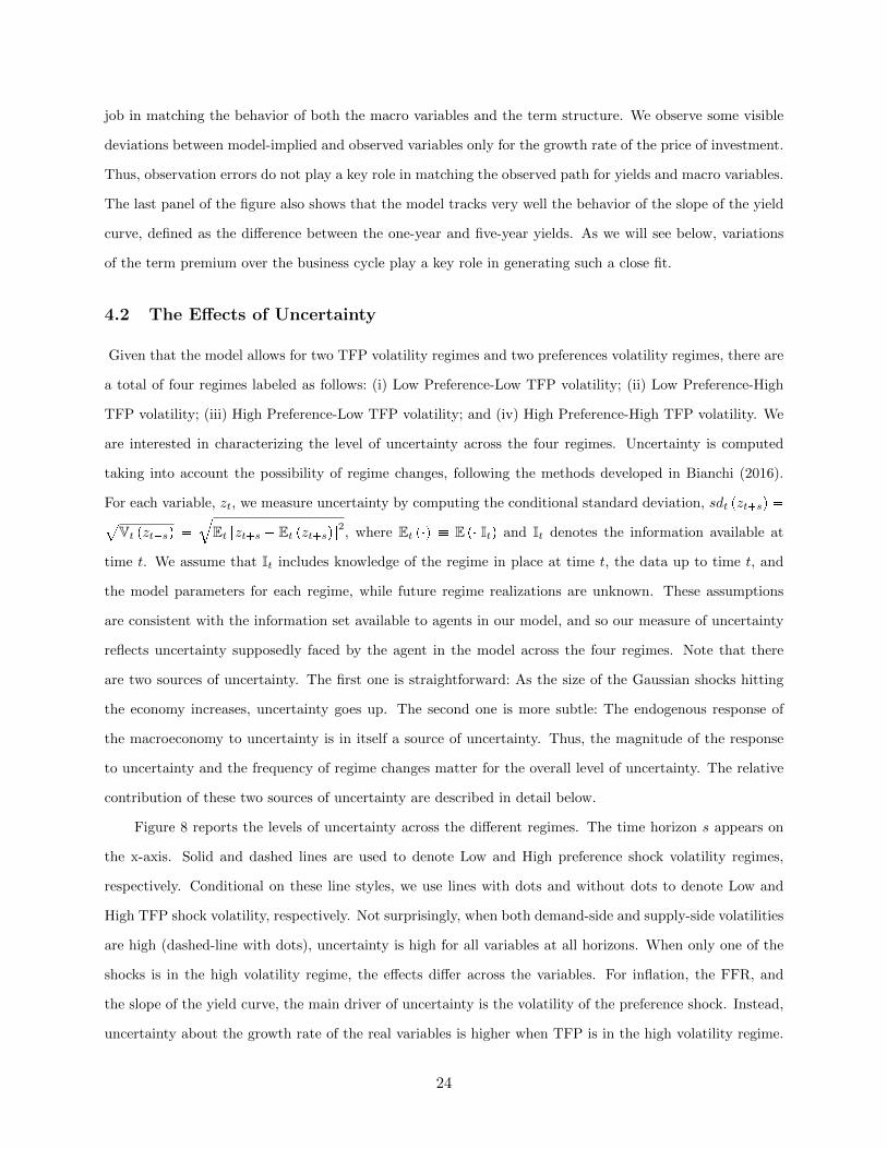
4.2 The Effects of Uncertainty

Given that the model allows for two TFP volatility regimes and two preferences volatility regimes, there are

a total of four regimes labeled as follows: (i) Low Preference-Low TFP volatility; (ii) Low Preference-High

TFP volatility; (iii) High Preference-Low TFP volatility; and (iv) High Preference-High TFP volatility. We

are interested in characterizing the level of uncertainty across the four regimes. Uncertainty is computed

taking into account the possibility of regime changes, following the methods developed in Bianchi (2016).

For each variable, zt, we measure uncertainty by computing the conditional standard deviation, sdt pzt�sq �aVt pzt�sq �

bEt rzt�s � Et pzt�sqs2, where Et p�q � E p�|Itq and It denotes the information available at

time t. We assume that It includes knowledge of the regime in place at time t, the data up to time t, and

the model parameters for each regime, while future regime realizations are unknown. These assumptions

are consistent with the information set available to agents in our model, and so our measure of uncertainty

reflects uncertainty supposedly faced by the agent in the model across the four regimes. Note that there

are two sources of uncertainty. The first one is straightforward: As the size of the Gaussian shocks hitting

the economy increases, uncertainty goes up. The second one is more subtle: The endogenous response of

the macroeconomy to uncertainty is in itself a source of uncertainty. Thus, the magnitude of the response

to uncertainty and the frequency of regime changes matter for the overall level of uncertainty. The relative

contribution of these two sources of uncertainty are described in detail below.

Figure 8 reports the levels of uncertainty across the different regimes. The time horizon s appears on

the x-axis. Solid and dashed lines are used to denote Low and High preference shock volatility regimes,

respectively. Conditional on these line styles, we use lines with dots and without dots to denote Low and

High TFP shock volatility, respectively. Not surprisingly, when both demand-side and supply-side volatilities

are high (dashed-line with dots), uncertainty is high for all variables at all horizons. When only one of the

shocks is in the high volatility regime, the effects differ across the variables. For inflation, the FFR, and

the slope of the yield curve, the main driver of uncertainty is the volatility of the preference shock. Instead,

uncertainty about the growth rate of the real variables is higher when TFP is in the high volatility regime.

24

It is also interesting to notice that uncertainty for consumption and GDP is slightly hump-shaped when

the High TFP volatility regime prevails. In other words, when TFP volatility is high, uncertainty is not

monotonically increasing with the time horizon, as agents are more uncertain about the short-run than the

long-run. This is because two competing forces are at play. On the one hand, events that are further into

the future are naturally harder to predict, as the possibility of shocks and regime changes increase. On the

other hand, in the long run, the probability of still being in the high volatility regime declines.

Figure 9 presents a simulation to understand the impact of these changes in uncertainty on business

cycle fluctuations and the term structure. We take the most likely regime sequence, as presented in Figure

6, and simulate the economy based on the parameters at the posterior mode, setting all Gaussian shocks to

zero. The top left panel reports the cyclical behavior of GDP and the slope of the yield curve implied by

the model. An increase in uncertainty produces a drop in real activity and an increase in the slope of the

yield curve, which consequently generates negative comovement between the slope of the yield curve and

real activity, as in the data (e.g., Ang, Piazzesi, and Wei (2006)). The four panels in the second and third

row of the figure compare the movements in the slope, GDP, consumption, and investment, induced by the

increase in uncertainty, with the business cycle fluctuations of the actual series. The estimated sequence of

the volatility regimes produces business cycle fluctuations and changes in the slope of the yield curve in a

way that closely tracks the observed fluctuations in the data.

The fluctuations in uncertainty also lead to significant breaks in the term premium. Term premium is

defined as the difference between the yield on a 5-year bond and the expected average short-term yield (1

quarter) over the same five years (following Rudebusch, Sack, and Swanson (2006)). The expected value

is computed taking into account the possibility of regime changes using the methods developed in Bianchi

(2016). The top-right panel of Figure 9 shows that both supply-side and demand-side uncertainty lead to an

increase in the term premium. Specifically, Table 4 shows that the nominal (real) term premia associated

with the different regimes are: (1) Low Preference - Low TFP volatility: 0.58% (0.33%); (2) Low Preference

- High TFP volatility: 0.84% (0.60%); (3) High Preference - Low TFP volatility: 1.03% (0.51%); and (4)

High Preference - High TFP volatility: 1.29% (0.78%). In Subsection 4.4, the mechanisms that lead to these

sizeable premia are explored in detail. For now, we are highlighting that term premia are large and vary

considerably in response to changes in uncertainty.

Our estimated model allows for a rich set of shocks to avoid forcing the estimation to artificially attribute

a large role to the uncertainty shocks. The results presented above suggest that uncertainty shocks can in

fact lead to sizeable fluctuations for both the macroeconomy and bond risk premia. In order to formally

quantify the importance of uncertainty shocks with respect to the other disturbances, we proceed in two

25

steps. First, we compute a variance decomposition by comparing the unconditional variance, as implied by

the model when only one shock is active, to the overall variance. Second, we explore how much variation

in endogenous variables at business cycle frequencies can be generated by uncertainty shocks. We do this

by computing the volatility of business cycle fluctuations in an economy where only uncertainty shocks are

present and comparing it to the volatility of business cycle fluctuations in an economy where both uncertainty

and level shocks are active.7

The decomposition of the unconditional variance for the observables is reported in the left panel of

Table 2. The results confirm that uncertainty shocks play an important role in explaining fluctuations in

the slope of the yield curve (28% of the unconditional variance), but they also account for a large fraction

of the variability of consumption and investment growth (14.26% and 9.67%, respectively). The right panel

of Table 2 highlights that uncertainty shocks appear even more important if we focus on their ability to

generate sizable business cycle fluctuations. Uncertainty shocks explain a substantial part of the variation

in consumption, investment, and output over the business cycle. In particular 24.52% of the variation in

consumption and around 31% of the variation in investment at business cycle frequencies can be explained

by uncertainty shocks. Finally, uncertainty shocks also explain 38.44% of business cycle variation in the

slope of the yield curve, confirming the evidence presented in Figure 9.

Finally, the variance decomposition in the left panel of Table 2 shows that the combination of TFP

shocks, preference shocks, and their corresponding volatility shocks accounts for a very large fraction of the

volatility of the macroeconomy and bond yields. Specifically, these shocks combined account for more than

80% of the variance of GDP growth, for more than 90% of the variance of consumption growth, for more

than 85% of the variance of investment growth, and for almost 60% of the variance of inflation and the slope

of the term structure of interest rates. The only other shock that plays a significant role is the markup shock.

However, this shock only appears to account for high-frequency movements in the volatility of inflation, as

it is often the case in estimated New-Keynesian models. Thus, the combination of first and second moments

shocks to TFP and preferences account for the bulk of the volatility of the observed variables, despite the

fact that we allow for a series of other shocks, like the liquidity shock, that generally play a significant role in

the estimation of New-Keynesian DSGE models without the risk-adjustment. This suggests that extending

standard estimation technique to include the first-order effects of uncertainty shocks can significantly change

the importance of the other shocks, possibly allowing for more parsimonious models to explain the observed

fluctuations.

7From a technical point of view the contribution of uncertainty shocks is given by the amount of volatility generatedby the Markov-switching constant.

26

4.3 Inspecting the Mechanism

To better understand the mechanisms at work, we decompose the effects of the uncertainty shocks into the

five risk propagation channels that were discussed in the context of the simplified model of Section 2: Pre-

cautionary savings, investment risk premium, inflation risk premium, nominal pricing bias, and investment

adjustment. The results show that the origins of uncertainty are important to understand its effects.

Figure 10 presents the median and 90% error bands for the impulse responses to a demand-side (dashed

line) and a supply-side (solid line) uncertainty shock, while Figure 11 presents the median and 90% error

bands for the difference between these impulse responses. Impulse responses are computed as the change

in the expected path of the endogenous variables following an initial impulse, in line with the way impulse

responses are computed for shocks to levels. Specifically, these impulse responses assume a shift from low to

high uncertainty in the first period, but from that point on they are computed integrating out future regime

changes. Thus, the impulse responses are conceptually different from the simulations reported in Figure 9

where the posterior mode regime sequence was imposed.

Despite these technical differences that take into account uncertainty about the future regime path,

uncertainty shocks still emerge as a driving force of the business cycle. Both demand- and supply-side

uncertainty shocks generate positive comovement between consumption, investment, output, as there is an

economic contraction following heightened macroeconomic uncertainty. Also, higher uncertainty increases

the nominal and real slope and term premia, consistent with the observed dynamics in the data. However, a

supply-side uncertainty shock leads to a much larger decline in inflation. Furthermore, the recession generated

by a supply-side uncertainty shock is visibly larger, as confirmed by the first row of Figure 10. The effects

on term premia are also quantitatively different, with the supply-side uncertainty shock generating a smaller

increase in the nominal term premium and a larger increase in the real term premium.

Figure 12 decomposes the effect of uncertainty increases for preferences (Panel a) and in TFP (Panel b).

Note that, in contrast to the calibrated simplified model presented above, the precautionary savings channel

generates positive comovement between consumption, investment, and output. In our estimated model, the

magnitude of price adjustment costs is sufficiently high that it flips the sign of investment (due to a larger

downward shift in labor demand). However, while this channel plays a key role in driving consumption down

following an uncertainty shock, other channels play an equally important role to understand the effects of

uncertainty on the other macroeconomic variables.

When the economy experiences a supply-side uncertainty shock, the investment risk channel is equally

(and at certain horizons more) important than the precautionary savings channel in determining a decline

27

in investment. On the other hand, when the economy experiences a demand-side uncertainty shock, the

risk propagation channel works in the opposite direction and mitigates the decline in investment. Thus,

demand and supply uncertainty propagate differently through the investment risk premium channel. The

difference is determined by how the shadow value of capital responds to adverse demand and supply shocks

(figure 13). For the household, capital works as a hedge against adverse preference shocks, because the

return on investment is positive in a state of the world with high marginal utility of wealth (high SDF). The

opposite is true for a negative TFP shock, as the return on investment is negative in the high SDF state.

So, when supply side uncertainty increases, the effect of the investment risk premium channel is driven by

investment becoming riskier and households, keeping all else equal, optimally choosing to cut investment. In

contrast, when demand uncertainty increases, investment becomes less risky and the effect of this channel

is determined by the household choosing a relatively higher level of investment than it would choose if

investment risk premium remained constant.

Importantly, the net effect of demand-side uncertainty on investment is still negative because of the

combined effect of the precautionary savings and nominal pricing bias channels. Indeed, when the economy

experiences a demand-side uncertainty shock, the nominal pricing bias channel contributes to the decline in

consumption and investment. In response to an increase in demand-side uncertainty the nominal price bias

determines effects similar to a markup shock, given that it enters the New-Keynesian Phillips curve in an

isomorphic way. Inflation goes up, consumption and investment go down. This contributes to exacerbating

the recession while mitigating the effects on inflation.

The decomposition also helps in understanding why the response of inflation is so muted in the two

cases. In both cases, the precautionary savings channel determines deflationary pressure. However, following

a demand-side uncertainty shock the pricing bias channel essentially nullifies the effects on inflation, while

in the case of the supply-side uncertainty shock this channel plays a very little role. To understand why, it is

useful to revisit the impulse responses presented in Figure 13. Inflation experiences a persistent increase in

response to a demand shock, while a supply shock has very little quantitative impact on inflation dynamics.

As a result, the nominal pricing bias channel is not quantitatively important for supply side uncertainty:

Firms do not adjust their price-setting decision, as supply side uncertainty has limited impact on uncertainty

about future inflation. In contrast, the preference shock is an important driver of inflation dynamics, and

demand-side uncertainty directly translates into uncertainty about future inflation. Hence, the nominal

pricing bias is an important determinant of the economy’s response to demand-side uncertainty.

Finally the other two channels, inflation risk premium and investment adjustment, have small quanti-

tative effects.

28

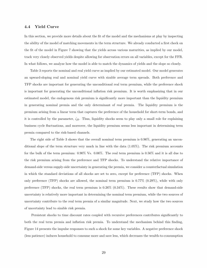
4.4 Yield Curve

In this section, we provide more details about the fit of the model and the mechanisms at play by inspecting

the ability of the model of matching movements in the term structure. We already conducted a first check on

the fit of the model in Figure 7 showing that the yields across various maturities, as implied by our model,

track very closely observed yields despite allowing for observation errors on all variables, except for the FFR.

In what follows, we analyze how the model is able to match the dynamics of yields and the slope so closely.

Table 3 reports the nominal and real yield curve as implied by our estimated model. Our model generates

an upward-sloping real and nominal yield curve with sizable average term spreads. Both preference and

TFP shocks are important for generating the unconditional real term premium, while the preference shock

is important for generating the unconditional inflation risk premium. It is worth emphasizing that in our

estimated model, the endogenous risk premium is significantly more important than the liquidity premium

in generating nominal premia and the only determinant of real premia. The liquidity premium is the

premium arising from a linear term that captures the preference of the household for short-term bonds, and

it is controlled by the parameter, ζB . Thus, liquidity shocks seem to play only a small role for explaining

business cycle fluctuations, and moreover, the liquidity premium seems less important in determining term

premia compared to the risk-based channels.

The right side of Table 3 shows that the overall nominal term premium is 0.96%, generating an uncon-

ditional slope of the term structure very much in line with the data (1.05%). The risk premium accounts

for the bulk of the term premium: 0.90% Vs. 0.06%. The real term premium is 0.56% and it is all due to

the risk premium arising from the preference and TFP shocks. To understand the relative importance of

demand-side versus supply-side uncertainty in generating the premia, we consider a counterfactual simulation

in which the standard deviations of all shocks are set to zero, except for preference (TFP) shocks. When

only preference (TFP) shocks are allowed, the nominal term premium is 0.77% (0.29%), while with only

preference (TFP) shocks, the real term premium is 0.26% (0.34%). These results show that demand-side

uncertainty is relatively more important in determining the nominal term premium, while the two sources of

uncertainty contribute to the real term premia of a similar magnitude. Next, we study how the two sources

of uncertainty lead to sizable risk premia.

Persistent shocks to time discount rates coupled with recursive preferences contributes significantly to

both the real term premia and inflation risk premia. To understand the mechanism behind this finding,

Figure 14 presents the impulse responses to such a shock for some key variables. A negative preference shock

(less patience) induces household to consume more and save less, which decreases the wealth-to-consumption

29

ratio. A drop in the wealth-to-consumption ratio implies a decline in the return on a claim to aggregate

consumption. When agents prefer an early resolution of uncertainty (ψ ¡ 1{γ), a decrease in the return on

the consumption claim increases marginal utility. When the shock is persistent, this leads to a sharp increase

in marginal utility. A persistent negative time preference shock also increases the real rate persistently, which

erodes the payoffs of long real bonds more than short ones. Given that a negative time preference shock is

associated with high marginal utility, long real bonds provide less insurance against bad states of the world

relative to short real bonds. In equilibrium, this helps to generate an upward-sloping real yield curve and a

positive real term premia, in a way similar to Albuquerque, Eichenbaum, Luo, and Rebelo (2016).

The time preference shock endogenously generates a negative relation between marginal utility and

inflation, which translates into positive inflation risk premia increasing with maturity. A persistent negative

time preference shock increases aggregate demand, which raises inflation persistently. The negative time

preference shock is also associated with high marginal utility as discussed above. Persistently higher inflation

erodes the value of long nominal bonds more than short nominal bonds during high marginal utility states.

Consequently, the nominal yield curve is upward-sloping.

The persistent TFP growth shocks in conjunction with habits contributes positively to real term pre-

mia. A negative TFP growth shock decreases consumption today relative to habit (proportional to lagged

consumption), decreasing surplus consumption (i.e., the difference between consumption and habits), and

raising marginal utility. However, next period, the habit catches up and increases expected surplus consump-

tion growth. This induces a borrowing motive to smooth surplus consumption, which therefore increases

the real rate akin to Wachter (2006). A persistent increase in the real rate erodes the value of long-term

real bonds more than short-term ones. Therefore long-term real bonds provide less insurance against high

marginal utility states induced by negative TFP shocks, which contributes to the upward-sloping real yield

curve and positive real term premia. However, the TFP shocks do not generate significant inflation risk

premia as TFP shocks have a very small effect on inflation (see Figure 13). Therefore, the impact of TFP

shocks on the nominal term premia are primarily through the real term premia component.

Table 4 illustrates how the dynamics of real and nominal term premia are driven by the preference

and TFP uncertainty shocks. As preference uncertainty shocks contribute significantly to the unconditional

real term premia and inflation risk premia, changes in demand-side uncertainty generates sizable variation

in the conditional real term premia and the conditional inflation risk premia. In contrast, TFP uncertainty

shocks mainly contribute to real term premia and not towards inflation risk premia since the level TFP

shocks mainly contribute to the unconditional real term premia. Quantitatively, changes in demand-side

uncertainty produce large fluctuations in term premia through the effects on inflation risk premia.

30

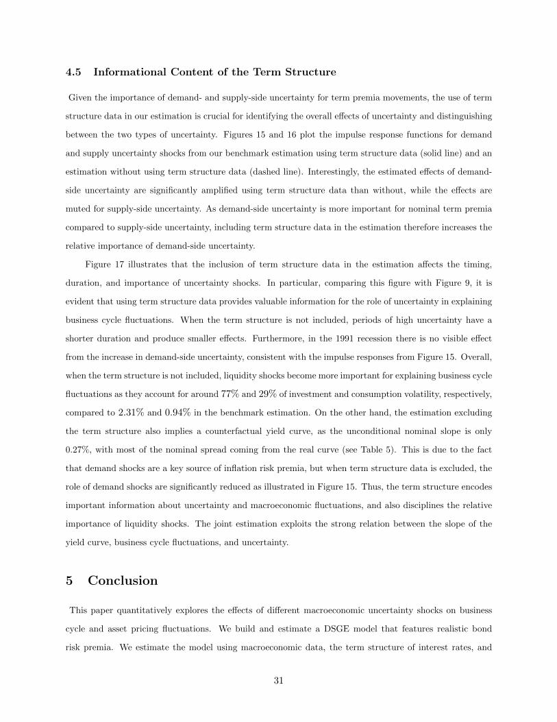
4.5 Informational Content of the Term Structure

Given the importance of demand- and supply-side uncertainty for term premia movements, the use of term

structure data in our estimation is crucial for identifying the overall effects of uncertainty and distinguishing

between the two types of uncertainty. Figures 15 and 16 plot the impulse response functions for demand

and supply uncertainty shocks from our benchmark estimation using term structure data (solid line) and an

estimation without using term structure data (dashed line). Interestingly, the estimated effects of demand-

side uncertainty are significantly amplified using term structure data than without, while the effects are

muted for supply-side uncertainty. As demand-side uncertainty is more important for nominal term premia

compared to supply-side uncertainty, including term structure data in the estimation therefore increases the

relative importance of demand-side uncertainty.

Figure 17 illustrates that the inclusion of term structure data in the estimation affects the timing,

duration, and importance of uncertainty shocks. In particular, comparing this figure with Figure 9, it is

evident that using term structure data provides valuable information for the role of uncertainty in explaining

business cycle fluctuations. When the term structure is not included, periods of high uncertainty have a

shorter duration and produce smaller effects. Furthermore, in the 1991 recession there is no visible effect

from the increase in demand-side uncertainty, consistent with the impulse responses from Figure 15. Overall,

when the term structure is not included, liquidity shocks become more important for explaining business cycle

fluctuations as they account for around 77% and 29% of investment and consumption volatility, respectively,

compared to 2.31% and 0.94% in the benchmark estimation. On the other hand, the estimation excluding

the term structure also implies a counterfactual yield curve, as the unconditional nominal slope is only

0.27%, with most of the nominal spread coming from the real curve (see Table 5). This is due to the fact

that demand shocks are a key source of inflation risk premia, but when term structure data is excluded, the

role of demand shocks are significantly reduced as illustrated in Figure 15. Thus, the term structure encodes

important information about uncertainty and macroeconomic fluctuations, and also disciplines the relative

importance of liquidity shocks. The joint estimation exploits the strong relation between the slope of the

yield curve, business cycle fluctuations, and uncertainty.

5 Conclusion

This paper quantitatively explores the effects of different macroeconomic uncertainty shocks on business

cycle and asset pricing fluctuations. We build and estimate a DSGE model that features realistic bond

risk premia. We estimate the model using macroeconomic data, the term structure of interest rates, and

31

imposing restrictions on the average investment risk premium. Our model allows for stochastic changes in

the volatility of demand-side (preferences) and supply-side (TFP) shocks, while at the same time controlling

for other disturbances often included in the estimation of New-Keynesian DSGE models. Uncertainty shocks

are triggered by changes in stochastic volatility, but the endogenous response of the macroeconomy to these

changes is in itself a source of uncertainty.

We study the effects of uncertainty through the lens of a novel decomposition that identifies five endoge-

nous risk propagation mechanisms: precautionary savings, investment risk premium, inflation risk premium,

nominal pricing bias, and investment adjustment channels. The effects arising from the investment and in-

flation risk premia channels are disciplined by the investment risk and nominal term premia, respectively.

We find sizable effects of changes in uncertainty. Both demand-side and supply-side generate a positive

comovement in consumption, investment, and output. The responses of inflation and term premia differ

depending on the source of uncertainty. Supply-side uncertainty leads to larger contractions in both invest-

ment and consumption. These differences are explained in light of the way uncertainty propagates through

the real economy. In response to an increase in supply-side uncertainty, an increase in the risk of investing in

physical capital contributes to determine a larger recession. Instead, when demand-side uncertainty is high,

investment in capital becomes more attractive, reducing the fall in investment. In response to an increase

in demand-side uncertainty, the negative effects on inflation from the precautionary savings channel are

nullified by a nominal bias in pricing. The joint estimation of macro and yield curve variables put additional

discipline on the relative importance of these channels, as the model is also asked to account for the negative

comovement between term premia and the macroeconomy. Overall, our results highlight the importance of

accounting for the origins of macroeconomic uncertainty and for using asset prices to discipline the various

risk propagation channels for uncertainty.

32

References

Albuquerque, R., M. Eichenbaum, V. X. Luo, S. Rebelo, 2016. Valuation risk and asset pricing.

The Journal of Finance 71(6), 2861–2904.

Ang, A., M. Piazzesi, M. Wei, 2006. What does the yield curve tell us about GDP growth?. Journal

of econometrics 131(1-2), 359–403.

Bachmann, R., C. Bayer, 2014. Investment dispersion and the business cycle. American Economic

Review 104(4), 1392–1416.

Backus, D. K., B. R. Routledge, S. E. Zin, 2010. Asset prices in business cycle analysis. Working

Paper.

Baker, S. R., N. Bloom, S. J. Davis, 2016. Measuring economic policy uncertainty. The Quarterly

Journal of Economics 131(4), 1593–1636.

Bansal, R., I. Shaliastovich, 2013. A long-run risks explanation of predictability puzzles in bond

and currency markets. Review of Financial Studies 26(1), 1–33.

Bansal, R., A. Yaron, 2004. Risks for the long run: A potential resolution of asset pricing puzzles.

The Journal of Finance 59(4), 1481–1509.

Basu, S., B. Bundick, 2017. Uncertainty shocks in a model of effective demand. Econometrica 85(3),

937–958.

Bekaert, G., S. Cho, A. Moreno, 2010. New Keynesian macroeconomics and the term structure.

Journal of Money, Credit and Banking 42(1), 33–62.

Bianchi, F., 2016. Methods for measuring expectations and uncertainty in Markov-switching models.

Journal of Econometrics 190(1), 79–99.

Bianchi, F., C. L. Ilut, M. Schneider, 2014. Uncertainty shocks, asset supply and pricing over the

business cycle. The Review of Economic Studies.

Bikbov, R., M. Chernov, 2010. No-arbitrage macroeconomic determinants of the yield curve. Jour-

nal of Econometrics 159(1), 166–182.

Blanchard, O. J., C. M. Kahn, 1980. The solution of linear difference models under rational expec-

tations. Econometrica: Journal of the Econometric Society pp. 1305–1311.

33

Bloom, N., 2009. The impact of uncertainty shocks. econometrica 77(3), 623–685.

Bloom, N., 2014. Fluctuations in uncertainty. Journal of Economic Perspectives 28(2), 153–76.

Bloom, N., M. Floetotto, N. Jaimovich, I. Saporta-Eksten, S. J. Terry, 2012. Really uncertain

business cycles. Unpublished working paper. National Bureau of Economic Research.

Bretscher, L., A. Hsu, A. Tamoni, 2017. Level and Volatility Shocks to Fiscal Policy: Term Structure

Implications. .

Campbell, J. Y., C. Pflueger, L. M. Viceira, 2014. Monetary policy drivers of bond and equity risks.

NBER Working Paper.

Cho, S., 2016. Sufficient conditions for determinacy in a class of Markov-switching rational expec-

tations models. Review of Economic Dynamics 21, 182–200.

Christiano, L. J., M. Eichenbaum, C. L. Evans, 2005. Nominal rigidities and the dynamic effects

of a shock to monetary policy. Journal of political Economy 113(1), 1–45.

Del Negro, M., F. Schorfheide, 2008. Forming Priors for DSGE Models (And How it Affects the

Assessment of Nominal Rigidities). 55(7), 1191–1208.

Den Haan, W. J., A. Marcet, 1994. Accuracy in simulations. The Review of Economic Studies

61(1), 3–17.

Dew-Becker, I., 2012. Essentially affine approximations for economic models. manuscript, June.

Dew-Becker, I., 2014. Bond pricing with a time-varying price of risk in an estimated medium-scale

bayesian DSGE model. Journal of Money, Credit, and Banking 46(5), 837–888.

Epstein, L., S. Zin, 1989. Substitution, risk aversion, and the temporal behavior of consumption

and asset returns: A theoretical framework. Econometrica 57(4), 937–69.

Fajgelbaum, P. D., E. Schaal, M. Taschereau-Dumouchel, 2017. Uncertainty traps. The Quarterly

Journal of Economics 132(4), 1641–1692.

Farmer, R. E., D. F. Waggoner, T. Zha, 2009. Understanding Markov-switching rational expecta-

tions models. Journal of Economic Theory 144(5), 1849–1867.

Farmer, R. E., D. F. Waggoner, T. Zha, 2011. Minimal State Variable Solution to Markov-Switching

Rational Expectations Models. Journal of Economic Dynamics and Control.

34

Fernandez-Villaverde, J., P. Guerron-Quintana, K. Kuester, J. Rubio-Ramırez, 2015. Fiscal volatil-

ity shocks and economic activity. American Economic Review 105(11), 3352–84.

Fernandez-Villaverde, J., P. Guerron-Quintana, J. F. Rubio-Ramırez, M. Uribe, 2011. Risk matters:

The real effects of volatility shocks. American Economic Review 101(6), 2530–61.

Foerster, A., J. F. Rubio-Ramırez, D. F. Waggoner, T. Zha, 2016. Perturbation methods for Markov-

switching dynamic stochastic general equilibrium models. Quantitative economics 7(2), 637–669.

Hamilton, J. D., 1989. A new approach to the economic analysis of nonstationary time series and

the business cycle. Econometrica: Journal of the Econometric Society pp. 357–384.

Hsu, A., E. X. Li, F. Palomino, 2014. Real and Nominal Equilibrium Yield Curves with Endogenous

Inflation: A Quantitative Assessment. .

Jermann, U. J., 1998. Asset pricing in production economies. Journal of monetary Economics 41(2),

257–275.

Jurado, K., S. C. Ludvigson, S. Ng, 2015. Measuring uncertainty. American Economic Review

105(3), 1177–1216.

Justiniano, A., G. E. Primiceri, 2008. The time-varying volatility of macroeconomic fluctuations.

American Economic Review 98(3), 604–41.

Kim, C.-J., C. R. Nelson, 1999. State-Space Models with Regime Switching. MIT Press, Cambridge,

Massachusetts.

Kimball, M. S., 1990. Precautionary Saving in the Small and in the Large. Econometrica: Journal

of the Econometric Society pp. 53–73.

Kung, H., 2015. Macroeconomic linkages between monetary policy and the term structure of interest

rates. Journal of Financial Economics 115(1), 42–57.

Lettau, M., 2003. Inspecting the mechanism: Closed-form solutions for asset prices in real business

cycle models. The Economic Journal 113(489), 550–575.

Ludvigson, S. C., S. Ma, S. Ng, 2018. Uncertainty and business cycles: exogenous impulse or

endogenous response?. Unpublished working paper. .

35

Malkhozov, A., 2014. Asset prices in affine real business cycle models. Journal of Economic Dy-

namics and Control 45, 180–193.

Piazzesi, M., M. Schneider, 2007. Equilibrium yield curves. NBER Macroeconomics Annual 2006,

Volume 21 pp. 389–472.

Rotemberg, J. J., 1982. Monopolistic price adjustment and aggregate output. The Review of Eco-

nomic Studies 49(4), 517–531.

Rudebusch, G., B. Sack, E. Swanson, 2006. Macroeconomic implications of changes in the term

premium. .

Rudebusch, G. D., E. T. Swanson, 2012. The bond premium in a DSGE model with long-run real

and nominal. American Economic Journal: Macroeconomics 4(1), 105–143.

Saijo, H., 2017. The uncertainty multiplier and business cycles. Journal of Economic Dynamics and

Control 78, 1–25.

Schaal, E., 2017. Uncertainty and unemployment. Econometrica 85(6), 1675–1721.

Sims, C. A., 2002. Solving linear rational expectations models. Computational economics 20(1),

1–20.

Sims, C. A., T. Zha, 2006. Were there regime switches in US monetary policy?. American Economic

Review 96(1), 54–81.

Uhlig, H., 2010. Easy EZ in DSGE. Working Paper.

Wachter, J. A., 2006. A consumption-based model of the term structure of interest rates. Journal

of Financial economics 79(2), 365–399.

Weber, M., 2015. Nominal rigidities and asset pricing. .

36

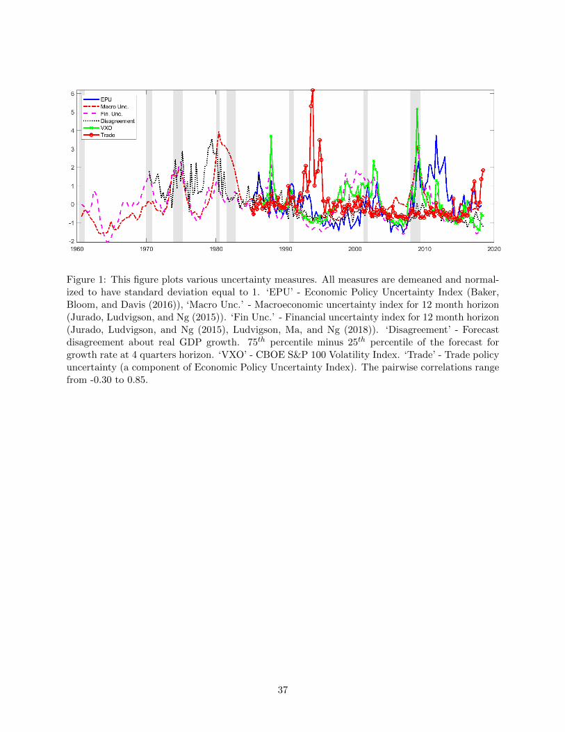
Figure 1: This figure plots various uncertainty measures. All measures are demeaned and normal-ized to have standard deviation equal to 1. ‘EPU’ - Economic Policy Uncertainty Index (Baker,Bloom, and Davis (2016)), ‘Macro Unc.’ - Macroeconomic uncertainty index for 12 month horizon(Jurado, Ludvigson, and Ng (2015)). ‘Fin Unc.’ - Financial uncertainty index for 12 month horizon(Jurado, Ludvigson, and Ng (2015), Ludvigson, Ma, and Ng (2018)). ‘Disagreement’ - Forecastdisagreement about real GDP growth. 75th percentile minus 25th percentile of the forecast forgrowth rate at 4 quarters horizon. ‘VXO’ - CBOE S&P 100 Volatility Index. ‘Trade’ - Trade policyuncertainty (a component of Economic Policy Uncertainty Index). The pairwise correlations rangefrom -0.30 to 0.85.

37

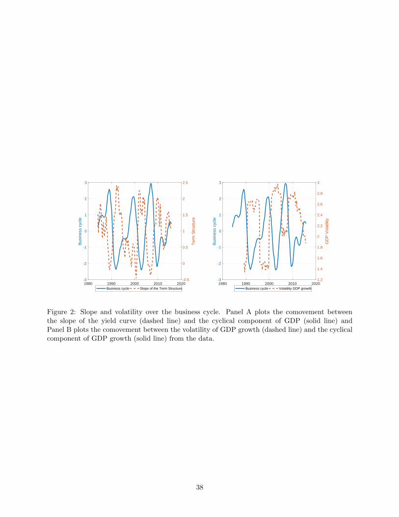
1980 1990 2000 2010 2020-3

-2

-1

0

1

2

3

Bus

ines

s cy

cle

-0.5

0

0.5

1

1.5

2

2.5

Ter

m S

truc

ture

Business cycle Slope of the Term Structure1980 1990 2000 2010 2020-3

-2

-1

0

1

2

3

Bus

ines

s cy

cle

1.2

1.4

1.6

1.8

2

2.2

2.4

2.6

2.8

3

GD

P V

olat

ility

Business cycle Volatility GDP growth

Figure 2: Slope and volatility over the business cycle. Panel A plots the comovement betweenthe slope of the yield curve (dashed line) and the cyclical component of GDP (solid line) andPanel B plots the comovement between the volatility of GDP growth (dashed line) and the cyclicalcomponent of GDP growth (solid line) from the data.

38

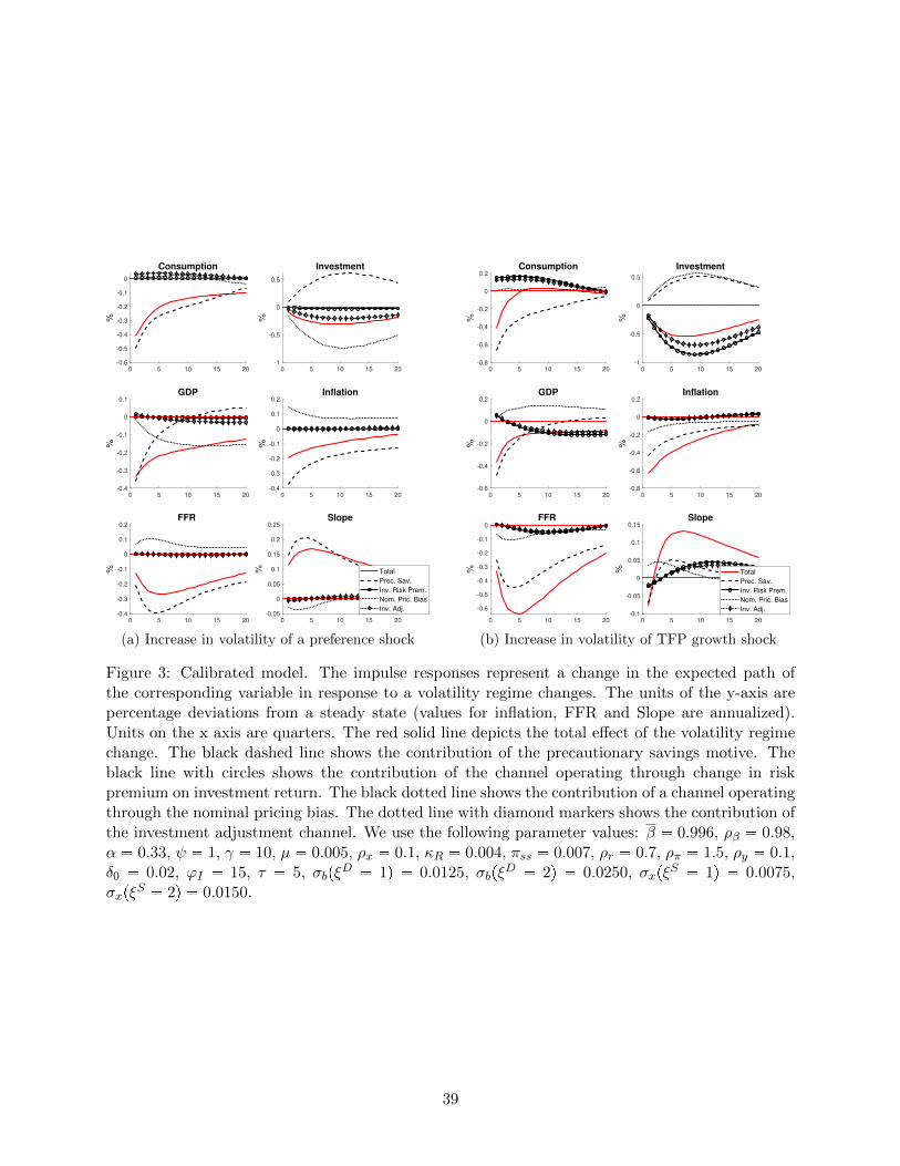
0 5 10 15 20-0.6

-0.5

-0.4

-0.3

-0.2

-0.1

0

%

Consumption

0 5 10 15 20-1

-0.5

0

0.5

%Investment

0 5 10 15 20-0.4

-0.3

-0.2

-0.1

0

0.1

%

GDP

0 5 10 15 20-0.4

-0.3

-0.2

-0.1

0

0.1

0.2

%

Inflation

0 5 10 15 20-0.4

-0.3

-0.2

-0.1

0

0.1

0.2

%

FFR

0 5 10 15 20-0.05

0

0.05

0.1

0.15

0.2

0.25

%

Slope

Total

Prec. Sav.

Inv. Risk Prem.

Nom. Pric. Bias

Inv. Adj.

(a) Increase in volatility of a preference shock

0 5 10 15 20-0.8

-0.6

-0.4

-0.2

0

0.2

%

Consumption

0 5 10 15 20-1

-0.5

0

0.5

%

Investment

0 5 10 15 20-0.6

-0.4

-0.2

0

0.2

%

GDP

0 5 10 15 20-0.8

-0.6

-0.4

-0.2

0

0.2

%

Inflation

0 5 10 15 20

-0.6

-0.5

-0.4

-0.3

-0.2

-0.1

0

%

FFR

0 5 10 15 20-0.1

-0.05

0

0.05

0.1

0.15

%

Slope

Total

Prec. Sav.

Inv. Risk Prem.

Nom. Pric. Bias

Inv. Adj.

(b) Increase in volatility of TFP growth shock

Figure 3: Calibrated model. The impulse responses represent a change in the expected path ofthe corresponding variable in response to a volatility regime changes. The units of the y-axis arepercentage deviations from a steady state (values for inflation, FFR and Slope are annualized).Units on the x axis are quarters. The red solid line depicts the total effect of the volatility regimechange. The black dashed line shows the contribution of the precautionary savings motive. Theblack line with circles shows the contribution of the channel operating through change in riskpremium on investment return. The black dotted line shows the contribution of a channel operatingthrough the nominal pricing bias. The dotted line with diamond markers shows the contribution ofthe investment adjustment channel. We use the following parameter values: β � 0.996, ρβ � 0.98,α � 0.33, ψ � 1, γ � 10, µ � 0.005, ρx � 0.1, κR � 0.004, πss � 0.007, ρr � 0.7, ρπ � 1.5, ρy � 0.1,δ0 � 0.02, ϕI � 15, τ � 5, σbpξ

D � 1q � 0.0125, σbpξD � 2q � 0.0250, σxpξ

S � 1q � 0.0075,σxpξ

S � 2q � 0.0150.

39

0 5 10 15 20

-0.005

0

0.005

0.01

0.015

0.02

0.025

%

Consumption

0 5 10 15 20

0

0.01

0.02

0.03

0.04

0.05

0.06

%

Investment

0 5 10 15 20

0

0.005

0.01

0.015

0.02

%

GDP

0 5 10 15 20

0

0.005

0.01

0.015

0.02

0.025

0.03

%

Inflation

0 5 10 15 20

0

0.005

0.01

0.015

0.02

0.025

0.03

%

FFR

0 5 10 15 20

-10

-5

0

5

%

10-3 Slope

Infl. Risk Prem.

(a) Increase in volatility of a preference shock

0 5 10 15 20

-0.03

-0.025

-0.02

-0.015

-0.01

-0.005

0

%

Consumption

0 5 10 15 20

-0.06

-0.05

-0.04

-0.03

-0.02

-0.01

0

%

Investment

0 5 10 15 20

-0.03

-0.025

-0.02

-0.015

-0.01

-0.005

0

%

GDP

0 5 10 15 20

-0.03

-0.025

-0.02

-0.015

-0.01

-0.005

0

%

Inflation

0 5 10 15 20

-0.04

-0.03

-0.02

-0.01

0

%

FFR

0 5 10 15 20

-5

0

5

10

%

10-3 Slope

Infl. Risk Prem.

(b) Increase in volatility of TFP growth shock

Figure 4: Calibrated model: Inflation risk premium channel of uncertainty. The impulse responsesrepresent a change in the expected path of the corresponding variables when volatility regimechanges. The units of the y-axis are percentage deviations from a steady state (values for inflation,FFR and Slope are annualized). Units on the x axis are quarters. We use the following parametervalues: β � 0.996, ρβ � 0.98, α � 0.33, ψ � 1, γ � 10, µ � 0.005, ρx � 0.1, κR � 0.004,πss � 0.007, ρr � 0.7, ρπ � 1.5, ρy � 0.1, δ0 � 0.02, ϕI � 15, τ � 5, σbpξ

D � 1q � 0.0125,σbpξ

D � 2q � 0.0250, σxpξS � 1q � 0.0075, σxpξ

S � 2q � 0.0150.

40

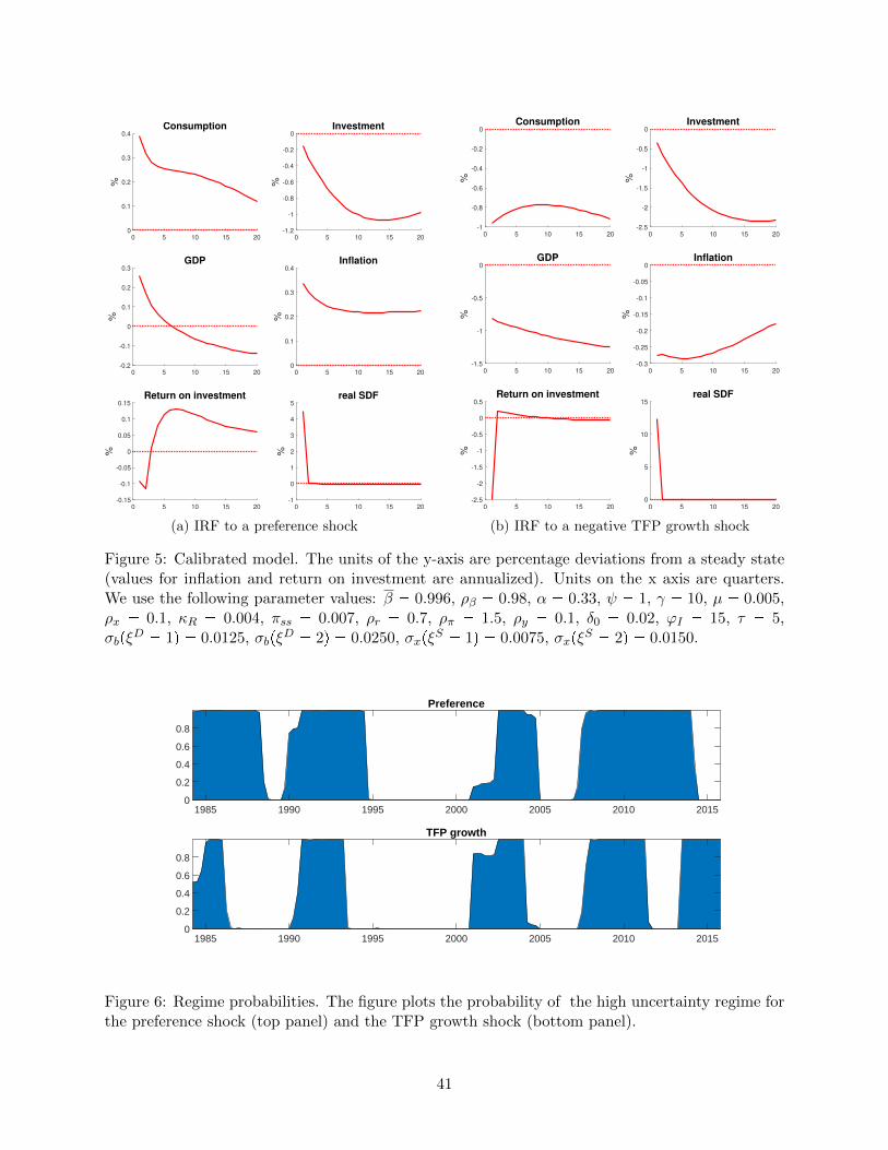
0 5 10 15 20

0

0.1

0.2

0.3

0.4

%

Consumption

0 5 10 15 20

-1.2

-1

-0.8

-0.6

-0.4

-0.2

0

%

Investment

0 5 10 15 20

-0.2

-0.1

0

0.1

0.2

0.3

%

GDP

0 5 10 15 20

0

0.1

0.2

0.3

0.4

%

Inflation

0 5 10 15 20

-0.15

-0.1

-0.05

0

0.05

0.1

0.15

%

Return on investment

0 5 10 15 20

-1

0

1

2

3

4

5

%

real SDF

(a) IRF to a preference shock

0 5 10 15 20

-1

-0.8

-0.6

-0.4

-0.2

0

%

Consumption

0 5 10 15 20

-2.5

-2

-1.5

-1

-0.5

0

%

Investment

0 5 10 15 20

-1.5

-1

-0.5

0

%

GDP

0 5 10 15 20

-0.3

-0.25

-0.2

-0.15

-0.1

-0.05

0

%

Inflation

0 5 10 15 20

-2.5

-2

-1.5

-1

-0.5

0

0.5

%

Return on investment

0 5 10 15 20

0

5

10

15

%

real SDF

(b) IRF to a negative TFP growth shock

Figure 5: Calibrated model. The units of the y-axis are percentage deviations from a steady state(values for inflation and return on investment are annualized). Units on the x axis are quarters.We use the following parameter values: β � 0.996, ρβ � 0.98, α � 0.33, ψ � 1, γ � 10, µ � 0.005,ρx � 0.1, κR � 0.004, πss � 0.007, ρr � 0.7, ρπ � 1.5, ρy � 0.1, δ0 � 0.02, ϕI � 15, τ � 5,σbpξ

D � 1q � 0.0125, σbpξD � 2q � 0.0250, σxpξ

S � 1q � 0.0075, σxpξS � 2q � 0.0150.

Preference

1985 1990 1995 2000 2005 2010 20150

0.2

0.4

0.6

0.8

TFP growth

1985 1990 1995 2000 2005 2010 20150

0.2

0.4

0.6

0.8

Figure 6: Regime probabilities. The figure plots the probability of the high uncertainty regime forthe preference shock (top panel) and the TFP growth shock (bottom panel).

41

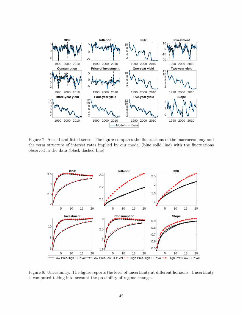
1990 2000 2010

-5

0

5GDP

1990 2000 2010

-5

0

5Inflation

1990 2000 2010

2468

10FFR

1990 2000 2010-20

-10

0

10Investment

1990 2000 2010

-2024

Consumption

1990 2000 2010

-5

0

5

Price of investment

1990 2000 2010

2468

10

One-year yield

1990 2000 2010

2468

1012

Two-year yield

1990 2000 2010

2468

1012

Three-year yield

1990 2000 2010

2468

1012

Four-year yield

1990 2000 2010

2468

1012

Five-year yield

1990 2000 2010

0

1

2

Slope

Model Data

Figure 7: Actual and fitted series. The figure compares the fluctuations of the macroeconomy andthe term structure of interest rates implied by our model (blue solid line) with the fluctuationsobserved in the data (black dashed line).

5 10 15 20

2

2.5

3

3.5GDP

5 10 15 20

2.1

2.2

2.3Inflation

5 10 15 20

1

1.5

2

2.5

FFR

5 10 15 20

6

8

10

Investment

5 10 15 201.5

2

2.5

3Consumption

5 10 15 20

0.5

0.6

0.7

0.8

0.9

Slope

Low Pref-High TFP vol Low Pref-Low TFP vol High Pref-High TFP vol High Pref-Low TFP vol

Figure 8: Uncertainty. The figure reports the level of uncertainty at different horizons. Uncertaintyis computed taking into account the possibility of regime changes.

42

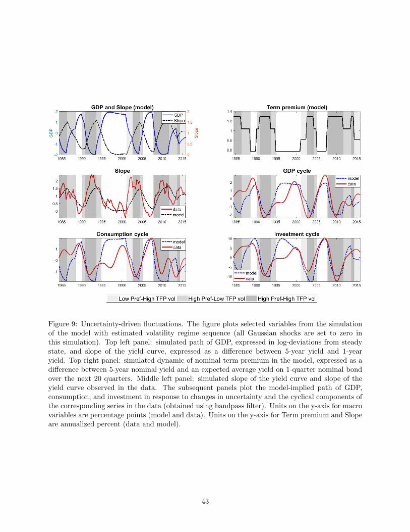
Figure 9: Uncertainty-driven fluctuations. The figure plots selected variables from the simulationof the model with estimated volatility regime sequence (all Gaussian shocks are set to zero inthis simulation). Top left panel: simulated path of GDP, expressed in log-deviations from steadystate, and slope of the yield curve, expressed as a difference between 5-year yield and 1-yearyield. Top right panel: simulated dynamic of nominal term premium in the model, expressed as adifference between 5-year nominal yield and an expected average yield on 1-quarter nominal bondover the next 20 quarters. Middle left panel: simulated slope of the yield curve and slope of theyield curve observed in the data. The subsequent panels plot the model-implied path of GDP,consumption, and investment in response to changes in uncertainty and the cyclical components ofthe corresponding series in the data (obtained using bandpass filter). Units on the y-axis for macrovariables are percentage points (model and data). Units on the y-axis for Term premium and Slopeare annualized percent (data and model).

43

Figure 10: Responses to uncertainty shocks. This figure plots impulse responses to a change fromlow uncertainty regime to high uncertainty regime for preference and TFP growth shocks. Thegray areas represent 90% credible sets. The impulse responses are computed as the change inthe expected path of the corresponding variables when the volatility regime changes. The figureplots impulse responses of consumption, investment, GDP, inflation, Fed Funds Rate (1-quarternominal interest rate), the slope of the yield curve expressed as the difference between 5-year and1-year nominal yields, nominal term premium defined as the difference between 5-year nominalyield and an expected average yield on 1-quarter nominal bond over the next 20 quarters, the realterm premium defined as the difference between 5-year real yield and an expected average yield on1-quarter real bond over the next 20 quarters, the real slope expressed as the difference between5-year and 1-year real yields. The units of the y-axis are percentage deviations from a steadystate (values for inflation, interest rates and term premia are annualized). Units on the x axis arequarters.

44

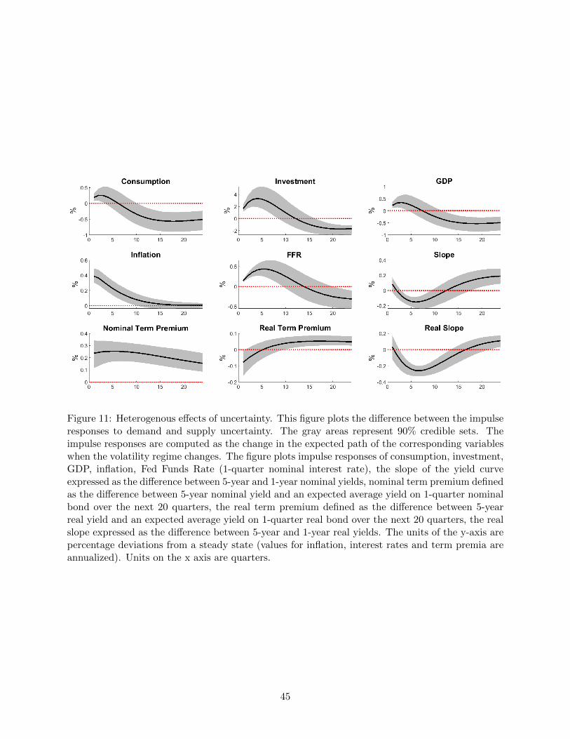
Figure 11: Heterogenous effects of uncertainty. This figure plots the difference between the impulseresponses to demand and supply uncertainty. The gray areas represent 90% credible sets. Theimpulse responses are computed as the change in the expected path of the corresponding variableswhen the volatility regime changes. The figure plots impulse responses of consumption, investment,GDP, inflation, Fed Funds Rate (1-quarter nominal interest rate), the slope of the yield curveexpressed as the difference between 5-year and 1-year nominal yields, nominal term premium definedas the difference between 5-year nominal yield and an expected average yield on 1-quarter nominalbond over the next 20 quarters, the real term premium defined as the difference between 5-yearreal yield and an expected average yield on 1-quarter real bond over the next 20 quarters, the realslope expressed as the difference between 5-year and 1-year real yields. The units of the y-axis arepercentage deviations from a steady state (values for inflation, interest rates and term premia areannualized). Units on the x axis are quarters.

45

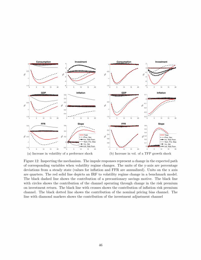
0 5 10 15 20-1.5

-1

-0.5

0

%

Consumption

0 5 10 15 20-6

-4

-2

0

2

4%

Investment

0 5 10 15 20-1.5

-1

-0.5

0

%

GDP

0 5 10 15 20

-0.4

-0.2

0

0.2

0.4

0.6

%

Inflation

0 5 10 15 20-1.5

-1

-0.5

0

0.5

%

FFR

0 5 10 15 20-0.2

0

0.2

0.4

0.6

%

Slope

Total

Prec. Sav.

Inv. Risk Prem.

Nom. Pric. Bias

Inv. Adj.

Infl. Risk Prem.

(a) Increase in volatility of a preference shock

0 5 10 15 20-1.5

-1

-0.5

0

%

Consumption

0 5 10 15 20-8

-6

-4

-2

0

2

%

Investment

0 5 10 15 20-1.5

-1

-0.5

0

%

GDP

0 5 10 15 20-0.4

-0.3

-0.2

-0.1

0

0.1

%

Inflation

0 5 10 15 20

-1

-0.8

-0.6

-0.4

-0.2

0

%

FFR

0 5 10 15 20

0

0.1

0.2

0.3

0.4

0.5

0.6

%

Slope

Total

Prec. Sav.

Inv. Risk Prem.

Nom. Pric. Bias

Inv. Adj.

Infl. Risk Prem.

(b) Increase in vol. of a TFP growth shock

Figure 12: Inspecting the mechanism. The impule responses represent a change in the expected pathof corresponding variables when volatility regime changes. The units of the y-axis are percentagedeviations from a steady state (values for inflation and FFR are annualized). Units on the x axisare quarters. The red solid line depicts an IRF to volatility regime change in a benchmark model.The black dashed line shows the contribution of a precautionary savings motive. The black linewith circles shows the contribution of the channel operating through change in the risk premiumon investment return. The black line with crosses shows the contribution of inflation risk premiumchannel. The black dotted line shows the contribution of the nominal pricing bias channel. Theline with diamond markers shows the contribution of the investment adjustment channel

46

(a) IRF to a preference shock (b) IRF to a negative TFP growth shock

Figure 13: Impulse responses to level preference and TFP shocks. The units of the y-axis arepercentage deviations from a steady state (values for inflation and return on investment are annu-alized). Units on the x axis are quarters.

Figure 14: IRF to a preference shock and term premium. The units of the y-axis are percentagedeviations from a steady state (values for inflation are annualized). Units on the x axis are quarters.The top left panel plots βt - loading on continuation utility in Epstein - Zin value function.

47

0 5 10 15 20 25 30-1.5

-1

-0.5

0

%Consumption

0 5 10 15 20 25 30-4

-3

-2

-1

0

%

Investment

0 5 10 15 20 25 30-1.5

-1

-0.5

0

%

GDP

0 5 10 15 20 25 300

0.02

0.04

0.06

%

Inflation

0 5 10 15 20 25 30-0.8

-0.6

-0.4

-0.2

0

%

FFR

0 5 10 15 20 25 300

0.1

0.2

0.3

0.4

%

Slope

0 5 10 15 20 25 300

0.1

0.2

0.3

0.4

%

Nominal Term Premium

0 5 10 15 20 25 300

0.05

0.1

0.15

0.2%

Real Term Premium

0 5 10 15 20 25 30-0.2

0

0.2

0.4

%

Real Slope

Demand Unc. Benchamrk Demand Unc. No asset price data

Figure 15: Effects of demand-side uncertainty when removing the term structure. This figure plotsthe impulse responses to a demand-side uncertainty shock based on the benchmark estimation(solid line) and in an alternative estimation without the term structure (dashed line).

0 5 10 15 20 25 30-1.5

-1

-0.5

0

%

Consumption

0 5 10 15 20 25 30

-6

-4

-2

0

2

%

Investment

0 5 10 15 20 25 30-2

-1.5

-1

-0.5

0

%GDP

0 5 10 15 20 25 30-0.4

-0.3

-0.2

-0.1

0

%

Inflation

0 5 10 15 20 25 30

-2

-1.5

-1

-0.5

0

%

FFR

0 5 10 15 20 25 30

0

0.5

1

%

Slope

0 5 10 15 20 25 300

0.2

0.4

0.6

0.8

%

Nominal Term Premium

0 5 10 15 20 25 300

0.2

0.4

0.6

0.8

%

Real Term Premium

0 5 10 15 20 25 30-0.5

0

0.5

1

%

Real Slope

Supply Unc. Benchmark Supply Unc. No asset price data

Figure 16: Effects of supply-side uncertainty when removing the term structure. This figure plotsthe impulse responses to a supply-side uncertainty shock based on the benchmark estimation (solidline) and in an alternative estimation without the term structure (dashed line).

48

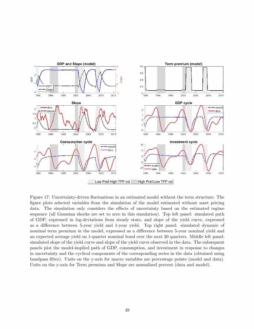
Figure 17: Uncertainty-driven fluctuations in an estimated model without the term structure. Thefigure plots selected variables from the simulation of the model estimated without asset pricingdata. The simulation only considers the effects of uncertainty based on the estimated regimesequence (all Gaussian shocks are set to zero in this simulation). Top left panel: simulated pathof GDP, expressed in log-deviations from steady state, and slope of the yield curve, expressedas a difference between 5-year yield and 1-year yield. Top right panel: simulated dynamic ofnominal term premium in the model, expressed as a difference between 5-year nominal yield andan expected average yield on 1-quarter nominal bond over the next 20 quarters. Middle left panel:simulated slope of the yield curve and slope of the yield curve observed in the data. The subsequentpanels plot the model-implied path of GDP, consumption, and investment in response to changesin uncertainty and the cyclical components of the corresponding series in the data (obtained usingbandpass filter). Units on the y-axis for macro variables are percentage points (model and data).Units on the y-axis for Term premium and Slope are annualized percent (data and model).

49

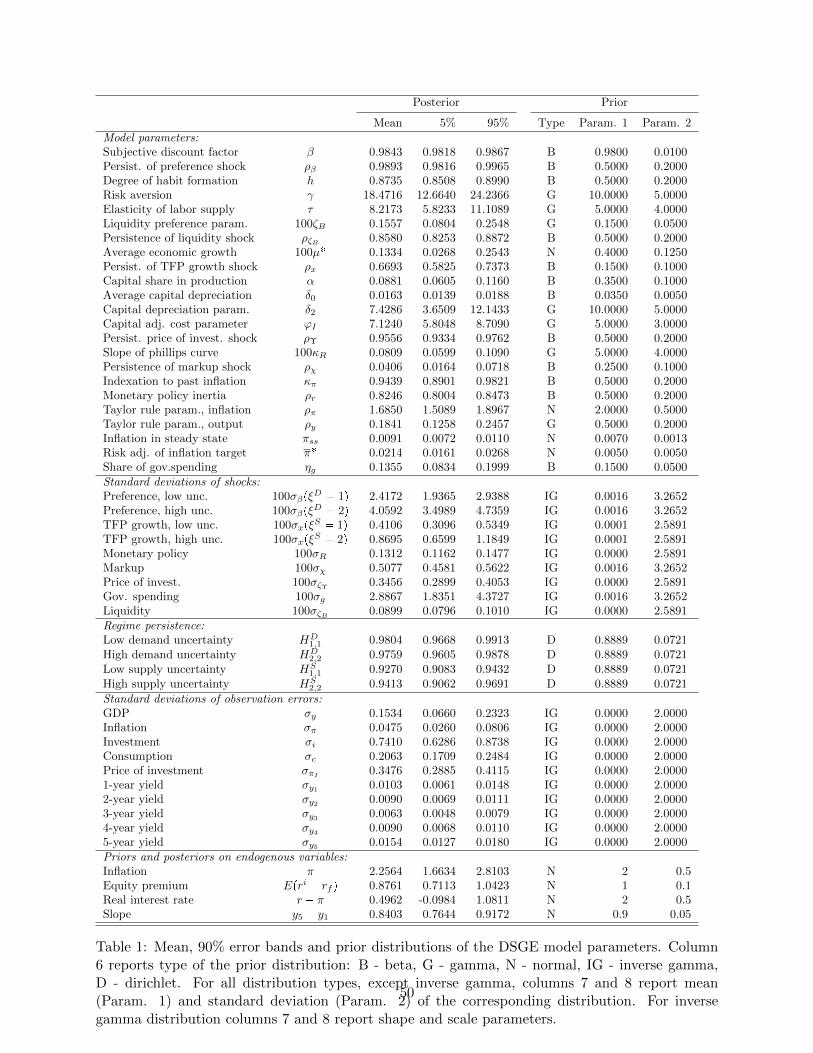
Posterior Prior

Mean 5% 95% Type Param. 1 Param. 2Model parameters:Subjective discount factor β 0.9843 0.9818 0.9867 B 0.9800 0.0100Persist. of preference shock ρβ 0.9893 0.9816 0.9965 B 0.5000 0.2000Degree of habit formation h 0.8735 0.8508 0.8990 B 0.5000 0.2000Risk aversion γ 18.4716 12.6640 24.2366 G 10.0000 5.0000Elasticity of labor supply τ 8.2173 5.8233 11.1089 G 5.0000 4.0000Liquidity preference param. 100ζB 0.1557 0.0804 0.2548 G 0.1500 0.0500Persistence of liquidity shock ρζB 0.8580 0.8253 0.8872 B 0.5000 0.2000Average economic growth 100µ� 0.1334 0.0268 0.2543 N 0.4000 0.1250Persist. of TFP growth shock ρx 0.6693 0.5825 0.7373 B 0.1500 0.1000Capital share in production α 0.0881 0.0605 0.1160 B 0.3500 0.1000Average capital depreciation δ0 0.0163 0.0139 0.0188 B 0.0350 0.0050Capital depreciation param. δ2 7.4286 3.6509 12.1433 G 10.0000 5.0000Capital adj. cost parameter ϕI 7.1240 5.8048 8.7090 G 5.0000 3.0000Persist. price of invest. shock ρΥ 0.9556 0.9334 0.9762 B 0.5000 0.2000Slope of phillips curve 100κR 0.0809 0.0599 0.1090 G 5.0000 4.0000Persistence of markup shock ρχ 0.0406 0.0164 0.0718 B 0.2500 0.1000Indexation to past inflation κπ 0.9439 0.8901 0.9821 B 0.5000 0.2000Monetary policy inertia ρr 0.8246 0.8004 0.8473 B 0.5000 0.2000Taylor rule param., inflation ρπ 1.6850 1.5089 1.8967 N 2.0000 0.5000Taylor rule param., output ρy 0.1841 0.1258 0.2457 G 0.5000 0.2000Inflation in steady state πss 0.0091 0.0072 0.0110 N 0.0070 0.0013Risk adj. of inflation target π� 0.0214 0.0161 0.0268 N 0.0050 0.0050Share of gov.spending ηg 0.1355 0.0834 0.1999 B 0.1500 0.0500Standard deviations of shocks:Preference, low unc. 100σβpξ

D � 1q 2.4172 1.9365 2.9388 IG 0.0016 3.2652Preference, high unc. 100σβpξ

D � 2q 4.0592 3.4989 4.7359 IG 0.0016 3.2652TFP growth, low unc. 100σxpξ

S � 1q 0.4106 0.3096 0.5349 IG 0.0001 2.5891TFP growth, high unc. 100σxpξ

S � 2q 0.8695 0.6599 1.1849 IG 0.0001 2.5891Monetary policy 100σR 0.1312 0.1162 0.1477 IG 0.0000 2.5891Markup 100σχ 0.5077 0.4581 0.5622 IG 0.0016 3.2652Price of invest. 100σζΥ 0.3456 0.2899 0.4053 IG 0.0000 2.5891Gov. spending 100σg 2.8867 1.8351 4.3727 IG 0.0016 3.2652Liquidity 100σζB 0.0899 0.0796 0.1010 IG 0.0000 2.5891Regime persistence:Low demand uncertainty HD

1,1 0.9804 0.9668 0.9913 D 0.8889 0.0721High demand uncertainty HD

2,2 0.9759 0.9605 0.9878 D 0.8889 0.0721Low supply uncertainty HS

1,1 0.9270 0.9083 0.9432 D 0.8889 0.0721High supply uncertainty HS

2,2 0.9413 0.9062 0.9691 D 0.8889 0.0721

Standard deviations of observation errors:GDP σy 0.1534 0.0660 0.2323 IG 0.0000 2.0000Inflation σπ 0.0475 0.0260 0.0806 IG 0.0000 2.0000Investment σi 0.7410 0.6286 0.8738 IG 0.0000 2.0000Consumption σc 0.2063 0.1709 0.2484 IG 0.0000 2.0000Price of investment σπI 0.3476 0.2885 0.4115 IG 0.0000 2.00001-year yield σy1

0.0103 0.0061 0.0148 IG 0.0000 2.00002-year yield σy2

0.0090 0.0069 0.0111 IG 0.0000 2.00003-year yield σy3

0.0063 0.0048 0.0079 IG 0.0000 2.00004-year yield σy4

0.0090 0.0068 0.0110 IG 0.0000 2.00005-year yield σy5 0.0154 0.0127 0.0180 IG 0.0000 2.0000Priors and posteriors on endogenous variables:Inflation π 2.2564 1.6634 2.8103 N 2 0.5Equity premium Epri � rf q 0.8761 0.7113 1.0423 N 1 0.1Real interest rate r � π 0.4962 -0.0984 1.0811 N 2 0.5Slope y5 � y1 0.8403 0.7644 0.9172 N 0.9 0.05

Table 1: Mean, 90% error bands and prior distributions of the DSGE model parameters. Column6 reports type of the prior distribution: B - beta, G - gamma, N - normal, IG - inverse gamma,D - dirichlet. For all distribution types, except inverse gamma, columns 7 and 8 report mean(Param. 1) and standard deviation (Param. 2) of the corresponding distribution. For inversegamma distribution columns 7 and 8 report shape and scale parameters.

50

Unconditional variance Uncertaintydecomposition and business cycle

Preference TFP growth Monetary Markup Uncertainty Median Conf. Inter.GDP 2.60 71.67 1.10 1.78 6.69 23.19 (16.49; 31.15)Inflation 31.62 0.06 0.04 67.72 0.49 14.47 (11.60; 17.88)FFR 79.13 1.65 4.46 7.22 6.42 38.26 (29.58; 48.10)Investment 2.56 70.27 2.56 4.40 16.05 33.76 (24.15; 45.88)Consumption 4.27 78.64 1.48 2.36 9.05 23.86 (17.35; 32.50)Slope 16.41 9.43 16.29 27.70 24.75 38.73 (30.43; 47.61)

Table 2: The left panel presents the contribution of the different shocks to the unconditionalvariance of the macroeconomic variables and the slope of the yield curve. The right panel analyzesthe importance of uncertainty shocks in generating business cycle fluctuations with respect tothe traditional level shocks. Specifically, we use the posterior mode parameter values to simulatetwo economies 1,000 times. In the first economy, only uncertainty shocks occur. In the secondeconomy, we have level shocks on top of the same uncertainty shocks. For each simulation andfor each variable we extract business cycle fluctuations using a bandpass filter. Finally, for eachsimulation we compute the ratio between the volatilities of the business cycle fluctuations for thetwo economies.

Yields Slope

1Q 1Y 2Y 3Y 4Y 5Y Total Risk Liquidity Only Pref. Only TFPNominal 2.77 2.88 3.08 3.31 3.53 3.72 0.95 0.89 0.06 0.63 0.41Real 0.57 0.58 0.71 0.89 1.06 1.21 0.63 0.63 - 0.22 0.43

Table 3: The left panel reports unconditional means of nominal and real yields in the estimatedmodel for the following maturities: 1-quarter and 1,2,3,4,5 years. The right panel reports theslopes of the corresponding term structures, defined as the difference between yields on 5-yearand 1-quarter bonds. The first column in the right panel reports the total value, while the nexttwo columns decompose the difference between 5-year and 1-quarter yield into risk premium andliquidity premium. The last two columns report the slope of the term structure in a model withonly preference shocks and only TFP growth shocks. Values are annualized percent. The 1-quarterreal yield corresponds to the risk free rate rf,t in the model. Real bond prices are computed as

Ppnqr,t � EtrMt�1P

pn�1qr,t�1 s, where Mt�1 is a real SDF.

Uncertainty regimePreference uncertainty Low Low High HighTFP growth uncertainty Low High Low High

Nominal Term Premium 0.57 0.82 1.04 1.29Real Term Premium 0.40 0.67 0.59 0.86Inflation Risk Premium 0.17 0.15 0.44 0.42

Table 4: This table reports nominal and real term premia conditional on the uncertainty regime.The term premium in the model is computed as the difference between 5-year yield and the expectedaverage yield on 1-quarter bond over the next 20 quarters. The inflation risk premium refers to thedifference between nominal and real term premia

51

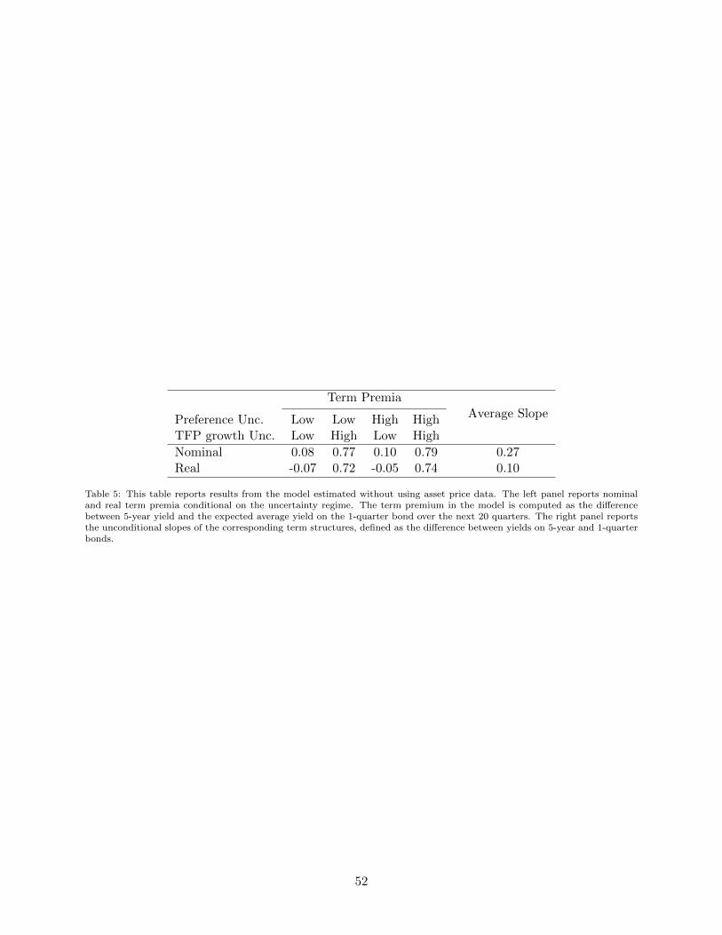
Term PremiaAverage SlopePreference Unc. Low Low High High

TFP growth Unc. Low High Low High

Nominal 0.08 0.77 0.10 0.79 0.27Real -0.07 0.72 -0.05 0.74 0.10

Table 5: This table reports results from the model estimated without using asset price data. The left panel reports nominaland real term premia conditional on the uncertainty regime. The term premium in the model is computed as the differencebetween 5-year yield and the expected average yield on the 1-quarter bond over the next 20 quarters. The right panel reportsthe unconditional slopes of the corresponding term structures, defined as the difference between yields on 5-year and 1-quarterbonds.

52

A Appendix. First order conditions from the estimated model

The household’s intertemporal condition is

1 � Et

�Mt�1

PtPt�1

�Rt �

1

Z�t

ζBerζB,tpCt � hCt�1q (64)

where

Mt�1 �1 � βt�1

1 � βtβt

��� Vt�1�EtV

1�γt�1

11�γ

�� 1�γ �

upCt�1, Lt�1, Bt�2q

upCt, Lt, Bt�1q

�1 �u11pCt�1, Lt�1, Bt�2q

u11pCt, Lt, Bt�1q

(65)

is the stochastic discount factor. The intratemporal condition is

Wt � τ0Lτt pCt � hCt�1q

First order conditions of the household with respect to a capital utilization choice and investment decision

result in the following two equations:

rktδ1pUtq

�1 � ϕI

2

�ItIt�1

� eµ�

Υ2

� ϕI

�ItIt�1

� eµ�

Υ

ItIt�1

��

�Et

�Mt�1

rkt�1

δ1pUt�1qϕI

�It�1

It� eµ

�

ΥI2t�1

I2t

�� peζΥ,tΥtq�1

rktδ1pUtq

� Et

�Mt�1

�rkt�1Ut�1 �

rkt�1

δ1pUt�1q

�1 � δpUt�1q

�FOC of the intermediate firm i with respect to the price setting decision:

�1 �

1�λp,tλp,t

�Pi,tPt

� 1�λp,tλp,t Yt

Pt�Wt

Li,t1�α

�1�λp,tλp,t

�Pi,tPt

�11Pt

�φR

�Pi,t

Πκπss Πp1�κπqt�1 Pi,t�1

� 1

Yt

Πκπss Πp1�κπqt�1 Pi,t�1

� Et

�Mt�1φR

�Pi,t�1

Πκπss Πp1�κπqt Pi,t

� 1

Yt�1Pi,t�1

Πκπss Πp1�κπqt P 2

i,t

�� 0

FOC of the intermediate firm i with respect to the capital choice:

rkt �α

1 � αWt

Li,tKi,t

53

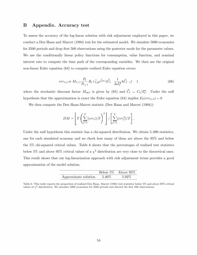
B Appendix. Accuracy test

To assess the accuracy of the log-linear solution with risk adjustment employed in this paper, we

conduct a Den Haan and Marcet (1994) test for the estimated model. We simulate 5000 economies

for 3500 periods and drop first 500 observations using the posterior mode for the parameter values.

We use the conditionally linear policy functions for consumption, value function, and nominal

interest rate to compute the time path of the corresponding variables. We then use the original

non-linear Euler equation (64) to compute realized Euler equation errors:

errt�1�M t�1PtPt�1

Rt�ζBerζB,tp pCt� 1

∆Z�th pCt�1q � 1 (66)

where the stochastic discount factor Mt�1 is given by (65) and pCt � Ct{Z�t . Under the null

hypothesis that the approximation is exact the Euler equation (64) implies Etperrt�1q � 0

We then compute the Den Haan-Marcet statistic (Den Haan and Marcet (1994)):

DM �

��T � T

s�1

perrsq{T

�2�� {

�T

s�1

perr2sq{T

�.

Under the null hypothesis this statistic has a chi-squared distribution. We obtain 5, 000 statistics,

one for each simulated economy and we check how many of them are above the 95% and below

the 5% chi-squared critical values. Table 6 shows that the percentages of realized test statistics

below 5% and above 95% critical values of a χ2 distribution are very close to the theoretical ones.

This result shows that our log-linearization approach with risk adjustment terms provides a good

approximation of the model solution.

Below 5% Above 95%

Approximate solution 5.40% 5.92%

Table 6: This table reports the proportion of realized Den Haan, Marcet (1994) test statistics below 5% and above 95% criticalvalues of χ2 distribution. We simulate 5000 economies for 3500 periods and discard the first 500 observations.

54