The Limited Macroeconomic Effects

of Unemployment Benefit Extensions

Gabriel Chodorow-Reich Harvard University and NBER

Loukas Karabarbounis

Federal Reserve Bank of Minneapolis, Chicago Booth, and NBER

Working Paper 733 April 2016

Keywords: Unemployment Insurance; Measurement Error; Unemployment JEL classification: E24, E62, J64, J65 The views expressed herein are those of the authors and not necessarily those of the Federal Reserve Bank of Minneapolis or the Federal Reserve System. __________________________________________________________________________________________

Federal Reserve Bank of Minneapolis • 90 Hennepin Avenue • Minneapolis, MN 55480-0291

https://www.minneapolisfed.org/research/

The Limited Macroeconomic Effects ofUnemployment Benefit Extensions∗

Gabriel Chodorow-ReichHarvard University and NBER

Loukas KarabarbounisFRB Minneapolis, Chicago Booth, and NBER

April 2016

Abstract

By how much does an extension of unemployment benefits affect macroeconomic

outcomes such as unemployment? Answering this question is challenging because U.S.

law extends benefits for states experiencing high unemployment. We use data revisions

to decompose the variation in the duration of benefits into the part coming from actual

differences in economic conditions and the part coming from measurement error in the

real-time data used to determine benefit extensions. Using only the variation coming

from measurement error, we find that benefit extensions have a limited influence on

state-level macroeconomic outcomes. We use our estimates to quantify the effects of

the increase in the duration of benefits during the Great Recession and find that they

increased the unemployment rate by at most 0.3 percentage point.

JEL-Codes: E24, E62, J64, J65.

Keywords: Unemployment Insurance, Measurement Error, Unemployment.

∗We are grateful to Ellen McGrattan, Emi Nakamura, and participants in seminars and conferences for helpful

comments. We thank Claudia Macaluso and Johnny Tang for excellent research assistance, Thomas Stengle of

the Department of Labor for help in understanding the unemployment insurance laws, and Bradley Jensen of

the Bureau of Labor Statistics for help in understanding the process for constructing state unemployment rates.

Karabarbounis thanks the Becker Friedman Institute at the University of Chicago and the Business and Public

Policy Faculty Research Fund at Chicago Booth for financial support. The views expressed herein are those of the

authors and not necessarily those of the Federal Reserve Bank of Minneapolis or the Federal Reserve System.

1 Introduction

Responding to the increase in unemployment during the Great Recession, the potential duration

of unemployment insurance (UI) benefits in the United States increased from 26 weeks to up

to 99 weeks. Recent studies have found small effects of these benefit extensions on individual

outcomes (Rothstein, 2011; Farber and Valletta, 2015). The effect on macroeconomic outcomes

has been more controversial. According to one view, by making unemployment relatively more

attractive to the jobless, the extension of benefits contributed substantially to the slow recovery

of the labor market (Barro, 2010; Mulligan, 2012; Hagedorn, Karahan, Manovskii, and Mitman,

2015). Others have emphasized the potential stimulus effects of increasing transfers to unem-

ployed individuals (Summers, 2010; Congressional Budget Office, 2012; Di Maggio and Kermani,

2015; Kekre, 2016). Distinguishing between these possibilities has important implications for

the design of UI policy and for economists’ understanding of labor markets.

Quantifying the effects of UI benefit extensions on macroeconomic outcomes is challenging.

Federal law links actual benefit extensions in a state directly to state-level macroeconomic con-

ditions. This policy rule mechanically generates a positive correlation between unemployment

and benefit extensions, complicating the identification of any direct effect that benefit extensions

may have on macroeconomic outcomes.

We combine a novel empirical research design with a standard labor market model augmented

with extensions of UI benefits to shed light on this policy debate. Our results are inconsistent

with either large negative or positive effects of benefit extensions on macroeconomic aggregates

including unemployment, employment, vacancies, and worker earnings. Instead, we find that

the extension of benefits has only a limited influence on macroeconomic outcomes.

Our empirical approach starts from the observation that, at the state level, the duration

of UI benefits depends on the unemployment rate as estimated in real time. However, real-

time data provide a noisy signal of the true economic fundamentals. It follows that two states

differ in the duration of their UI benefits because of differences in fundamentals or because

of measurement error. We use subsequent revisions of the unemployment rate to separate the

1

Table 1: April 2013 Example

Louisiana Wisconsin

Real-Time Data Unemployment Rate (Moving Average) 5.9% 6.9%

Duration of Benefit Extensions 14 Weeks 28 Weeks

Revised Data (2015) Unemployment Rate (Moving Average) 6.9% 6.9%

Duration of Benefit Extensions 28 Weeks 28 Weeks

UI Error -14 Weeks 0 Weeks

fundamentals from the measurement error. We then use the measurement error component of

UI benefit extensions to identify the effects of benefit extensions on state-level macroeconomic

aggregates. Effectively, our strategy exploits the randomness in the duration of benefits with

respect to economic fundamentals caused by measurement error in the fundamentals.

Table 1 uses the example of Louisiana and Wisconsin in April 2013 to illustrate our strategy.

Under the 2008 emergency compensation program, the duration of benefits in a state increased

by 14 additional weeks if a moving average of the state’s unemployment rate exceeded 6 percent.

The unemployment rate measured in real time in Louisiana was 5.9 percent while that in

Wisconsin was 6.9 percent, resulting in an additional 14 weeks of potential benefits in Wisconsin

relative to Louisiana. However, data revised as of 2015 show that both states actually had the

same unemployment rate of 6.9 percent. According to the revised data, both states should have

qualified for the additional 14 weeks. We refer to the 14 weeks that Louisiana did not receive

as a “UI error.” This error reflects mismeasurement of the economic fundamentals rather than

differences in fundamentals between the two states and, therefore, provides exogenous variation

to estimate the effects of UI benefit extensions on state aggregates. In the event, the actual

unemployment rate (from the revised data as of 2015) evolved very similarly following the UI

2

error, declining by roughly 0.2 percentage point between April and June 2013 in both states.

Our empirical exercise amounts to asking whether this apparent limited influence of extending

benefits on unemployment generalizes to a larger sample.

We begin our analysis in Section 2 by discussing relevant institutional details of the UI

system, the measurement of real-time and revised unemployment rates, and the UI errors that

arise because of differences between real-time and revised data. Similar to the example of

Louisiana and Wisconsin in April 2013, during the period 1996-2014 we find more than 600

state-month cases in which the duration of benefits using the revised data differs from the

actual duration of benefits. The great majority of these UI errors occur during the Great

Recession. This reflects both the additional tiers of benefits duration created by the 2008

emergency compensation program and the fact that most states experienced unemployment

rates high enough for measurement errors to affect their eligibility for extended benefits.

Once a UI error occurs, it takes on average nearly 4 months to revert to zero. Workers and

firms may adjust their behavior in response to past and current unexpected changes in the UI

error and to expectations about the future evolution of the error. We model the UI error as

a flexible Markov process and identify its unexpected component, which we call the “UI error

innovation.” Unlike the error itself, the innovation displays essentially zero serial correlation.

Our exercise then proceeds in two steps. First, we estimate the impulse response of state-level

variables to a UI error innovation. Then, we use a model matching these impulse responses

to show the evolution of macroeconomic aggregates when a negative shock brings the economy

into a recession in which agents anticipate extensions of benefits similar to those observed after

the Great Recession.

In Section 3 we present our main empirical findings. Innovations in the UI error have

negligible effects on state-level unemployment, employment, vacancies, and worker earnings.

In our baseline specification, a one-month positive innovation in the UI error generates at

most a 0.02 percentage point increase in the unemployment rate. Crucially, a positive UI

error innovation raises the fraction of the unemployed who claim UI benefits by a statistically

3

significant and an economically reasonable magnitude. Therefore, our results do not reflect the

fact that more unemployed do not claim benefits in response to a UI error. They simply reflect

the small macroeconomic effects of an increase in UI eligibility and receipt.

We validate our results along three dimensions. First, we show the robustness of our results

to the inclusion of a number of controls into the baseline specification, to alternative specifica-

tions, and to measurement error in the revised data. Second, we document that lags of variables

such as the unemployment rate do not predict UI error innovations. Third, the information con-

tent of the UI errors depends on the extent to which the revised unemployment rates measure

true economic conditions better than the real-time unemployment rates. Revisions in the un-

employment rate reflect better and more source data and methodological developments. We

illustrate the improvement in measurement by comparing the predictive power of real-time and

revised unemployment rates for actual consumer spending, new building permits issued, and

survey attitudes and beliefs. In horse-race regressions, we obtain positive loadings on revised

unemployment but not on real-time unemployment, indicating that the revised data better align

with agents’ decisions and perceptions of economic conditions in real time.

Our empirical estimates provide a direct answer to the question of what would happen if a

state increased the duration of unemployment benefits around the neighborhood of a typical UI

error, or by about 3 months after a state has already extended benefits by nearly one year. The

policy debate following the Great Recession has focused on the different, but related, question

of the macroeconomic effects of extending benefits all the way from 26 to as many as 99 weeks.

Extrapolating linearly the upper bound of our estimates, we find that extending benefits from

26 to 99 weeks increased the unemployment rate by at most 0.3 percentage point.

In Section 4 we use a model to further illustrate the informativeness of our empirical re-

sults for the effects of extending benefits on macroeconomic outcomes. Relative to the direct

calculation in the data, the model allows for potential non-linearities in the response of the

unemployment rate to benefit extensions and anticipation effects by workers and firms. We

augment the standard DMP framework (Diamond, 1982; Mortensen and Pissarides, 1994) with

4

a UI policy which determines benefit duration as the sum of two components. The first compo-

nent is the duration of UI benefits if unemployment were measured without any error. Mimicking

the actual UI law, eligible unemployed face an expected duration of benefits that increases in

the aggregate unemployment rate. The second component is an exogenous Markov process for

the UI error with transition probabilities drawn directly from the data. The remainder of the

model deviates minimally from the standard model in the literature in order to make our point

as transparent as possible.

The effect of UI policy on macroeconomic outcomes in the DMP model depends crucially

on the level of the opportunity cost of employment. We parameterize two model economies.

We denote by z = ξ + b the opportunity cost of employment, where ξ is the value of non-

market work and b is the value of benefits for the average unemployed. The first economy has

a high average level of z = ξ + b = 0.81 + 0.15 = 0.96 relative to a marginal product of one,

as advocated by Hagedorn and Manovskii (2008). The second economy has a lower average

level of z = ξ + b = 0.81 + 0.06 = 0.87. The value of b = 0.06 accords with the estimates of

Chodorow-Reich and Karabarbounis (2015) who show that benefits comprise a small fraction

of the average opportunity cost mainly because many unemployed do not receive these benefits.

We begin our theoretical analysis by tracing the model’s impulse responses to a one-month

UI error innovation. In the high b economy, the unemployment rate increases by roughly 0.15

percentage point, while in the low b economy the unemployment rate increases by less than

0.02 percentage point. The increase in unemployment in both economies reflects the fact that

benefit extensions raise the opportunity cost of working for the average unemployed which puts

upward pressure on wages, lowers firm profits, and dampens vacancy creation. The difference in

magnitude occurs because in the high b economy average firm profits are smaller and, therefore,

the increase in the opportunity cost decreases firms profits by more in percent terms. We

conclude that the low b model comes much closer than the high b model in matching the

empirical response of the unemployment rate to a one-month UI error innovation (less than

0.02 percentage point).

5

In the final step of our analysis, we subject both economies to a sequence of large negative

shocks that increase unemployment from below 6 percent to roughly 10 percent. Similar to what

happened during the Great Recession, the increase in unemployment triggers benefit extensions

in the model from 6 months to 20 months. To estimate the influence of benefit extensions

on the path of unemployment, we then subject the two economies to the same sequence of

shocks but without the benefit extensions. Removing benefit extensions in the high b model

reduces the average unemployment rate over a three-year horizon by 3.1 percentage points. The

corresponding number in the low b model is less than 0.3 percentage point. Because the low b

model matches the response of unemployment to a UI error innovation, we conclude that benefit

extensions play a limited role in increasing unemployment during a recession.1

Related Literature. The economic literature on the effects of benefit extensions has followed

two related lines of inquiry. Motivated in part by a partial equilibrium optimal taxation result

linking the optimal provision of UI to individual search behavior (Baily, 1978; Chetty, 2006), a

microeconomic literature has studied how various aspects of UI policy affects individual labor

supply (see for a survey Krueger and Meyer, 2002). Recent studies in this literature find a

small effect of benefit extensions on individual job finding rates and unemployment duration

(Rothstein, 2011; Farber and Valletta, 2015).2

The macroeconomic effects of UI benefits concern their effect on aggregate unemployment.3

Economic theory does not provide a one-to-one mapping between the magnitude of the microe-

conomic and macroeconomic effects. For example, in a standard DMP model with exogenous

job search effort and Nash bargaining, an increase in UI benefits raises workers’ outside options,

putting an upward pressure on wages and depressing firm vacancy creation. Exogenous search

1Our conclusion differs from the results of Mitman and Rabinovich (2014) who argue that benefit extensionsexplain jobless recoveries. Benefit extensions generate significant movements in unemployment only under veryhigh values of opportunity costs b and z. The small response of unemployment to a UI error innovation impliesthat b is much lower than the values generated by the Mitman and Rabinovich (2014) model.

2Schmieder, von Wachter, and Bender (2012) and Kroft and Notowidigdo (2015) show that the effect of UIbenefit extensions on unemployment duration becomes smaller during recessions. Johnston and Mas (2015) findsomewhat larger microeconomic effects than other recent studies.

3See Hansen and Imrohoroglu (1992), Krusell, Mukoyama, and Sahin (2010), and Nakajima (2012) for generalequilibrium analyses of unemployment insurance policy.

6

effort implies a zero microeconomic effect, but the decline in total vacancies generates a rise in

total unemployment, i.e. a non-zero macroeconomic effect (Hagedorn, Karahan, Manovskii, and

Mitman, 2015). Alternatively, in models with job rationing, large microeconomic effects could

be consistent with small macroeconomic effects if the job finding rate of UI recipients falls but

that of non recipients rises (Levine, 1993; Landais, Michaillat, and Saez, 2015; Lalive, Landais,

and Zweimuller, 2015).

In important contributions, Hagedorn, Karahan, Manovskii, and Mitman (2015) and Hage-

dorn, Manovskii, and Mitman (2015) use a county border discontinuity design to estimate a

large positive effect of UI benefit extensions on unemployment. Hall (2013) challenges aspects of

their research design and Amaral and Ice (2014) and Coglianese (2015) report that the results

are sensitive to changes in the specification. Johnston and Mas (2015) use a sudden change

in benefits in Missouri to estimate both the microeconomic and macroeconomic effects. They

estimate macroeconomic effects of similar magnitude to the microeconomic effects, but their

estimate of the macroeconomic effect depends on a difference-in-difference research design with

Missouri the only treated observation. Consistent with our findings, Marinescu (2015) docu-

ments a small effect of benefit duration on vacancies. In work closest in approach to our own,

Coglianese (2015) also recognizes that measurement error in the unemployment rate may help

to identify the macroeconomic effects of duration extensions. Our approach differs from his

in using the data revisions to isolate the measurement error in the duration of UI benefits, in

explicitly modeling a stochastic process for the measurement error, and in our interpretation of

the informativeness of our empirical estimates for key policy experiments through the lens of

the DMP model.4

2 Empirical Design

We begin this section by discussing relevant institutional details of the UI system and the

measurement of real-time and revised unemployment rates. We then define the UI errors that

4Our approach is also related to Suarez Serrato and Wingender (2014) who use data revisions to identify theeffects of government spending on state-level outcomes.

7

arise because of differences between real-time and revised data and discuss how we use these

errors to estimate the effects of UI benefit extensions on state-level aggregate outcomes.

2.1 Unemployment Insurance Laws

The maximum number of weeks of UI benefits available in the United States varies across

states and over time. Regular benefits in most states provide 26 weeks of compensation, with

a range between 13 and 30 weeks. The duration of regular UI benefits does not depend on

economic conditions in the state. Extended benefits (EB) and emergency compensation provide

additional weeks of benefits during periods of high unemployment in a state. The EB program

has operated since 1970 and is 50 percent federally funded except for the period 2009-2013

when it became fully federally funded. Emergency compensation programs are authorized and

financed on an ad hoc basis by the federal government. Our sample contains the Temporary

Emergency Unemployment Compensation (TEUC) program between March 2002 and December

2003 and the Emergency Unemployment Compensation (EUC) program between July 2008 and

December 2013. We refer to the combination of EB and emergency compensation as UI benefit

extensions.

Qualification for benefit extensions in a state typically depends on the unemployment rate

exceeding some threshold. Two measures of unemployment arise in the laws governing these

extensions. The insured unemployment rate (IUR) is the ratio of recipients of regular benefits

to employees covered by the UI system. The total unemployment rate (TUR) is the ratio of

the total number of individuals satisfying the official definition of not working and on layoff or

actively searching for work to the total labor force. To avoid very high frequency movements

in the available benefit extensions, both the IUR and the TUR enter into the trigger formulas

determining extensions as three-month moving averages. A trigger may also contain a lookback

provision which requires that the indicator exceed its value during the same set of months in

prior years. In Appendix A we list the full set of benefit extension programs, tiers, and triggers

in operation during our sample.

8

2.2 Measurement of State Unemployment and Data Revisions

Whether a state extends its duration of benefits or not depends on state-level estimates of the

IUR and TUR as estimated in real time. The real-time IUR uses as inputs administrative data

on UI payments and covered employment and, therefore, contains little measurement error. The

Local Area Unemployment Statistics (LAUS) program at the Bureau of Labor Statistics (BLS)

produces the state-level estimates of the TUR. Unlike the national unemployment rate, which

derives directly from counts from the Current Population Survey (CPS) of households, the state

unemployment rates incorporate auxiliary information to overcome the problem of small sample

sizes at the state level. Better source data and improved statistical models imply substantial

revisions in the estimated TUR over time.

We give here a brief description of BLS’s procedure to estimate state unemployment rates

and present more details in Appendix A. The real-time unemployment rate equals the ratio of

real-time unemployment to real-time unemployment plus employment. The BLS uses a state

space filter to estimate separately real-time total unemployment and total employment. For

unemployment the observed variables are the CPS count of unemployed individuals in the state

and the number of insured unemployed. For employment the observed variables are the CPS

count of employed individuals and the level of payroll employment in the state from the Current

Employment Statistics program. From 2005 to 2014, the procedure also included a real-time

benchmarking constraint that allocated pro rata the residual between the sum of filter-based

levels across states and the total at the Census division or national level. Finally, in 2009 the BLS

began applying a one-sided moving average filter to the state space filtered and benchmarked

data.

The BLS publishes revisions of its estimates of the state unemployment rates. The revisions

do not determine eligibility into the various extended benefits programs. Revisions occur for

three reasons. First, the auxiliary data used in the estimation – insured unemployment and

payroll employment – are updated with administrative data not available in real time. Second,

the BLS incorporates the entire time series available at the time of the revision into its model,

9

replacing the state space filter with a state space smoother and the one-sided moving-average

filter with a symmetric filter. Third, the BLS periodically updates its estimation procedure to

reflect methodological improvements. Most recently, in 2015 the BLS discontinued the external

real-time benchmarking constraint and incorporated a benchmarking constraint within the state

space model to reduce the spillover of state-specific noise in the CPS across states.

2.3 The UI Errors

We now explain how to construct the UI errors. Let Ts,t denote the actual duration of benefit

extensions in state s and month t, let Ts,t denote the hypothetical duration of benefit extensions

under the revised data, and let Ts,t denote the UI error. We define the UI error as the difference

between Ts,t and Ts,t:

Ts,t = Ts,t + Ts,t. (1)

Variation in the actual duration of benefit extensions Ts,t comes from the component Ts,t which

depends on the true economic fundamentals and from the component Ts,t which reflects mea-

surement error in the state unemployment rate. The key idea of our approach is to use variation

induced only from the UI error Ts,t to identify the effects of benefit extensions on state-level

outcomes.

We use the EB program in the state of Vermont to illustrate our measurement of the two

components. Figure 1 plots four lines. The blue solid step function shows the additional

weeks of benefits available to unemployed in Vermont in each calendar week, TVT,t. This series

depends on the real-time unemployment data, plotted by the dashed blue line. The red dashed

step function shows TVT,t, the additional weeks of benefits that would have been available in

Vermont using the revised unemployment rate series plotted by the dashed red line.

Vermont extended its benefits by an additional 13 weeks in the beginning of 2009. Because

the real-time and the revised unemployment rate move closely together in this period, Vermont

would have triggered an EB extension using either the real-time or the revised data as an input

in the trigger formula. The unemployment rate peaks at the end of 2009. As the unemployment

10

3.0

4.0

5.0

6.0

7.0

Un

em

plo

ym

en

t R

ate

0

13

20

Ad

ditio

na

l W

ee

ks A

va

ilab

le

2001 2002 2003 2004 2005 2006 2007 2008 2009 2010 2011 2012 2013 2014 2015

Real-Time Weeks Revised Weeks Real-Time U Revised U

Figure 1: Extended Benefits and Unemployment in Vermont

Notes: The figure plots the duration of benefits Ts,t and Ts,t (left axis) together with the real-time and revisedunemployment rates (right axis).

rate starts to decline, a UI error occurs. In the beginning of 2010, the real-time unemployment

rate temporarily increases by a small amount whereas the revised rate continues to decline

steadily. Under the revised data, EB should have been discontinued at the beginning of 2010.

However, under the real-time data, EB remained in place until roughly the middle of 2010.

The UI error, which is the difference between the blue and red step functions, takes the value

of 13 weeks during the first part of 2010. This error reflects mismeasurement of Vermont’s

unemployment rate in real time.

We next describe more formally how we separate Ts,t into the component Ts,t that corre-

sponds to the fundamentals and the UI error Ts,t. We start with a dataset containing the

information in the weekly trigger notices produced by the Department of Labor (DOL). The

DOL produces each week a trigger notice that contains for each state the most recent available

moving averages of IUR and TUR, the ratios of IUR and TUR relative to previous years, and

information on whether a state has any weeks of EB available and whether it has adopted op-

tional triggers for EB status. During periods with emergency compensation programs, the DOL

also produces separate trigger notices with the relevant input data and status determination

for the emergency programs. We scraped data for EB notices from 2003-2015 and for the EUC

11

Table 2: Accuracy of Our Algorithm for Calculating UI Benefit Extensions

EB TEUC02 EUC08 Total

Original Trigger NoticesCorrectly Imputed 45456 3982 14291 63729Incorrectly Imputed 44 18 9 71

Corrected Trigger NoticesCorrectly Imputed 45494 3999 14300 63793Incorrectly Imputed 6 1 0 7

Notes: The table reports counts of correct or incorrect predictions of UI benefit extensions in our algorithm relativeto the outcomes published by the DOL in its trigger notices. The counts are at the state-week level and coverthe period 1996-2014. The top panel compares our algorithm to the raw trigger notices. In the bottom panel, wehave corrected the information in the raw trigger notices when we find conflicting accounts in either contemporarymedia sources or in the text of state legislation.

2008 programs from the DOL’s online repository.5 The TEUC notices are not available online

but were provided to us by the DOL. Finally, the DOL library in Washington, D.C. contains

print copies of trigger notices before 2003, which we scanned and digitized.6 We augment these

data with monthly real-time unemployment rates by digitizing archived releases of the monthly

state and local unemployment reports from the BLS.

We use the revised unemployment data as of 2015 as inputs into the trigger formulas de-

scribed in Appendix Table A.1 to calculate Ts,t. The UI error then equals Ts,t = Ts,t − Ts,t.7

5The address is http://www.oui.doleta.gov/unemploy/claims_arch.asp.6The library could not locate notices for part of 1998. We also digitized notices for the EUC program in operation

between 1991 and 1994. However, we found only few non-zero UI errors. We, therefore, exclude this period fromour analysis and start in 1996, which is the year in which the BLS began using state space models to constructreal-time unemployment for all 50 states.

7States have the option to adopt or not two of the triggers for EB status. We follow the actual state lawsin determining whether to apply the optional triggers. A complication arises with a temporary change in thelaw between December 17, 2010 and December 31, 2013. The EB total unemployment rate trigger requires the(three-month) moving average of the unemployment rate in a state to exceed 120% of its level in the same periodin either of the two previous years. With unemployment in many states still high at the end of 2010 but no longerrising, Congress temporarily allowed states to pass laws extending the lookback period by an additional year. Manystates passed such laws in the week in which the two-year lookback period would have implied an expiration of EB.When we use the revised unemployment rate to construct the duration of benefits under the EB program, we findthat five states would have lost eligibility for EB earlier than in reality. Therefore, in constructing Ts,t, we assumethat states would have adopted the three-year lookback option earlier had the duration of benefits under the EBprogram followed the revised rather than the real-time unemployment rate. Specifically, we set to zero the UI errorfrom the EB program in any week in which a state had not adopted the three-year lookback trigger, the state dideventually adopt the three-year lookback trigger, and the UI error would have been zero had the state adopted the

12

To verify the accuracy of our algorithm for constructing Ts,t, we apply the same algorithm to

real-time data for Ts,t and compare the duration of extensions implied by our algorithm to the

actual duration reported in the trigger notices. Our algorithm does extremely well, as shown in

Table 2. Of 63,800 possible state-weeks, we correctly predict the duration in all but 7 cases.8

2.4 Innovations in UI Errors

The UI error Ts,t exhibits serial correlation, as shown for example in the Vermont case in Figure

1. This implies that firms and workers respond to past and current unexpected changes in the

UI error and to expectations about the future evolution of the error. We define the “UI error

innovation” as the current period unexpected component of the UI error:

εs,t = Ts,t − Et−1Ts,t, (2)

where Et−1Ts,t denotes the expectation of Ts,t using information available until period t− 1.

To identify the unexpected component in the UI error εs,t, we need to estimate the expecta-

tion of the future value of the UI error. We aggregate Ts,t up to a monthly frequency and assume

that it follows a first-order discrete Markov chain. Let πT

(Ts,t = xj | Ts,t−1 = xi;us,t, t

)be the

probability that T transits from a value xi to a value xj conditional on the unemployment rate

and calendar time. We allow the probabilities to depend on the unemployment rate and calendar

time because the mapping from a measurement error in the unemployment rate to a UI error

depends on whether the measurement error occurs in a region of the unemployment rate space

sufficiently close to a trigger threshold. For example, in the case of Vermont shown in Figure

1, measurement error in the mid-2000s does not cause a UI error because the unemployment

rate is far below the threshold for triggering an extension of benefits. Conditioning on calendar

three-year lookback trigger in that week. This change affects a negligible fraction of observations in our sample (atotal of 20 state-week observations).

8Our algorithm does better than the trigger notices, in the sense that it identifies more than 50 instanceswhere the trigger notices report an incorrect duration or aspect of UI law which we subsequently correct usingcontemporary local media sources or by referencing the actual text of state legislation. We suspect but cannotconfirm that the remaining discrepancies also reflect mistakes in the trigger notices. A number of previous papershave relied on information contained in the trigger notices (Rothstein, 2011; Hagedorn, Karahan, Manovskii, andMitman, 2015; Hagedorn, Manovskii, and Mitman, 2015; Marinescu, 2015; Coglianese, 2015). Our investigationreveals that, while small in number, uncorrected mistakes in the trigger notices could induce some attenuation bias.

13

time reflects the time variation in UI laws and triggers, for example due to the enactment of an

emergency compensation program.

We estimate each probability πT

(Ts,t = xj | Ts,t−1 = xi;us,t, t

)as the fraction of transitions

of the UI error from xi to xj for observations in the same unemployment rate and calendar time

bin. We form a vector of discrete possible values of x from one-half standard deviation wide

bins of Ts,t. Finally, once we have estimated the transition probabilities of the Markov process,

we calculate the expectation Et−1Ts,t and form the UI error innovation εs,t using equation (2).9

2.5 Summary Statistics of Variables Used in Analyses

We draw on a number of sources for state-level outcome variables. From the BLS, along with

the (revised) unemployment rate, we use monthly employment growth from the Current Em-

ployment Statistics program and monthly labor force participation from the LAUS program.

We obtain data on the number of UI claimants across all programs by state and month from the

DOL ETA 539 and ETA 5159 activity reports and from special tabulations for the July 2008

to December 2013 period.10 We obtain monthly data on vacancies from the Conference Board

Help Wanted Print Advertising Index and the Conference Board Help Wanted Online Index.

We use the first for the years 1996-2003 and aggregate local areas up to the state level. We use

the online index for 2007-2014. The print index continues until June 2008 and the online index

begins in 2005. However, the two indexes exhibit conflicting trends between 2004 and 2006 as

vacancy posting gradually transitioned from print to online, and we exclude this period from

our analysis of vacancies.11 Our measure of worker wages, available at quarterly frequency, is

the earnings of all and of new workers from the Census Bureau Quarterly Workforce Indicators.

9An obvious trade-off exists between finer partitioning of the state space and retaining sufficient observationsto make the exercise non-trivial. We estimate separate transition matrices for each of the following sequentialgroupings, motivated by the divisions shown in Table A.1: December 2008 – May 2012 and 5.5 ≤ us,t < 7;December 2008 – May 2012 and 7 ≤ us,t < 8.5; December 2008 – May 2012 and us,t ≥ 8.5; June 2012 – December2013 and 5.5 ≤ us,t < 7; June 2012 – December 2013 and 7 ≤ us,t < 9; June 2012 – December 2013 and us,t ≥ 9;January 2002 – December 2003 and us,t ≥ 5.5; us,t ≥ 5.5; us,t < 5.5. We have experimented with coarser groupings

and larger bins of Ts,t with little effect on our results.10These are found at http://www.ows.doleta.gov/unemploy/DataDownloads.asp and http:

//workforcesecurity.doleta.gov/unemploy/euc.asp respectively, last accessed February 10, 2016.11The loss of these years has little effect for our results because these years contain very few UI errors. See Sahin,

Song, Topa, and Violante (2014) for a description of the vacancy data and a comparison to JOLTS.

14

Table 3: Summary Statistics of Selected Variables

Variable Symbol Mean S.D.WithinS.D.

P(25) P(75) Obs.

Unemployment Rate Error (3 month m.a.) us,t −0.07 0.34 0.30 −0.27 0.10 11700Duration of Benefit Extensions Ts,t 3.32 5.46 1.44 0.00 3.50 11700

UI Error Ts,t 0.02 0.53 0.51 0.00 0.00 11700UI Error Innovation εs,t −0.00 0.34 0.33 −0.00 0.00 11550Unemployment Rate (Revised 2015) us,t 5.55 1.93 0.82 4.20 6.60 11700Fraction Unemployed Claiming UI φs,t 40.47 16.57 6.72 27.96 50.44 11550Log Vacancies (Detrended) log vs,t 0.04 0.27 0.16 −0.15 0.24 7656Log Payroll Employment (Detrended) logEs,t 0.00 0.03 0.02 −0.02 0.02 11700Log Earnings of All Workers (Detrended) logws,t 0.00 0.03 0.03 −0.02 0.02 3204Log Earnings of New Hires (Detrended) logws,t 0.00 0.05 0.04 −0.03 0.03 3066

Memo:

Duration of Benefit Extensions (Ts,t 6= 0) Ts,t 11.84 4.53 5.00 11.75 618

UI Error (Ts,t 6= 0) Ts,t 0.47 2.27 −1.50 2.25 618UI Error Innovation (εs,t 6= 0) εs,t 0.04 1.43 −1.03 0.97 643Length of Episode 3.86 3.13 2.00 4.00 161

Notes: All variables except for Log Earnings are measured at monthly frequency. Denoted variables have beendetrended with a state-specific linear time trend. Within S.D. is the standard deviation of the variable’s residualfrom a regression of the variable on state and month fixed effects.

Table 3 reports summary statistics. Our sample covers the period between 1996 and 2014

for the 50 U.S. states.12 The average error in the state total unemployment rate, which we

denote by us,t and define as the difference between the real-time unemployment rate and the

revised unemployment rate, is close to zero with a standard deviation of 0.34 percentage point.

Measurement error in the unemployment rate is spread across states and months as its standard

deviation changes little after controlling for state and month fixed effects.13

A potential concern with our empirical approach is that there are too few or too small errors

to identify significant effects of benefit extensions on macroeconomic outcomes. Table 3 shows

that this is not true. There are 618 cases in which a state would have had a different duration

12We exclude months in which a benefit extension program had temporarily lapsed for at least half the month(June 2010, July 2010, and December 2010) and the months immediately following (August 2010 and January2011).

13In contrast to the total unemployment rate, the insured unemployment rate contains almost no revisions. Thestandard deviation of the error in the insured unemployment rate is only 0.02 percentage point.

15

of extensions using the revised data. Conditional on a UI error occurring, that is Ts,t 6= 0, the

standard deviation of the UI error is larger than 2 months. The interquartile range is roughly

4 months. The fact that there is enough variation in the UI error relative to outcome variables

such as the unemployment rate explains the small standard errors of our estimates below.

The average episode of non-zero UI error lasts nearly 4 months and occurs when benefit

extensions already provide an additional year of UI eligibility. Most of these episodes occur

during the Great Recession. As already discussed in Section 2.4, measurement error in the

unemployment rate translates into a UI error only if the state’s unemployment rate is sufficiently

near a trigger threshold. This fact explains why we examine errors in the number of weeks

available T directly rather than measurement error in the unemployment rate. It also explains

why the UI errors occur mostly in the Great Recession, a period when both the EUC program

created additional trigger thresholds and most states had unemployment rates high enough for

measurement errors in the unemployment rate to translate into UI errors.

2.6 Summary of Empirical Design

Our strategy for overcoming the endogeneity of UI benefit extensions to macroeconomic condi-

tions has the following elements. First, we use data revisions to isolate the component of benefit

extensions arising from mismeasurement of state unemployment rates in real time. We denote

this component by Ts,t and find that such UI errors are common and persistent. Next, we

construct the unexpected component of the UI error, εs,t. The UI error innovation εs,t provides

variation across states and over time in UI benefit extensions which does not reflect variation in

macroeconomic conditions and, as we show below, exhibits essentially zero serial correlation.14

We proceed in two steps. In Section 3, we estimate the impulse response of state-level

variables to a UI error innovation εs,t and provide a model-free interpretation of the results. In

Section 4, we use a DMP model to show the informativeness of these impulses for macroeconomic

14Our strategy resembles a Regression Discontinuity (RD) framework, but with the crucial difference being thatUI errors reflect larger and more persistent variation than the variation RD uses around a trigger threshold. Usingour model, we find that when shocks are very persistent, a pure RD framework could fail to detect significant effectsof benefit extensions on unemployment despite the existence of such effects. See Appendix C for more details.

16

outcomes in response to shocks that trigger extensions of benefits similar to those observed after

the Great Recession.

3 Empirical Results

We measure the response of labor market variables to a one-month UI error innovation εs,t. Our

specification takes the form:

ys,t+h = β(h)εs,t + Γ(h)Xs,t + νs,t+h, (3)

where ys,t+h is an outcome variable in state s and period t+ h, εs,t is the UI error innovation in

state s and period t, and Xs,t is a vector of covariates. The coefficients β(h) for h = 0, 1, 2, ...

trace out the impulse response function of y with respect to a one-month unexpected change in

the UI error. In our baseline specification, Xs,t contains only a state fixed effect ds and a month

fixed effect dt. We include state and month fixed effects because, as seen in Table 3, they absorb

substantial variation in our main outcome variables and, therefore, improve the precision of our

estimates. In robustness checks reported below, we either exclude the fixed effects or include

additional covariates such as the measurement error in the unemployment rate us,t and lags of

the unemployment rate. In all specifications, we cluster standard errors by state and by month.

3.1 Main Results

Figure 2 shows impulse responses of the innovation ε and the UI error T to a one-month

innovation ε. As expected, the innovation exhibits essentially no serial correlation.15 The UI

error T rises one-for-one with ε on impact and then decays over the next few months with a

half-life of roughly 2 months. In all impulses, dashed lines report the 90 percent confidence

interval.

Figure 3 shows an increase in the fraction of the unemployed claiming UI benefits in response

to a positive one-month UI error innovation. Upon impact, the fraction of unemployed claiming

15The lack of serial correlation provides support for our choice of modeling T as a first-order Markov process.Time aggregation from weekly to monthly frequency could induce some serial correlation between months t andt+ 1, as an increase in T in week 3 or 4 of month t would produce a positive innovation in both t and t+ 1.

17

Response of ε

-.2

0

.2

.4

.6

.8

1

1.2

Inno

vatio

n in

UI D

urat

ion

Err

or

0 2 4 6 8 10 12

Response of T

-.2

0

.2

.4

.6

.8

1

1.2

Cha

nge

in U

I Dur

atio

n E

rror

0 2 4 6 8 10 12

Figure 2: Serial Correlation

Notes: The figure plots the coefficients on εs,t from the regressions εs,t+h = β(h)εs,t + ds(h) + dt(h) + νs,t+h and

Ts,t+h = β(h)εs,t + ds(h) + dt(h) + νs,t+h. The dashed lines denote the 90 percent confidence interval based ontwo-way clustered standard errors.

-1

-.5

0

.5

1

Chan

ge in

Fra

ction

Clai

ming

UI (

PP)

0 2 4 6 8 10 12

Figure 3: Impulse Response of Fraction Claiming UI

Notes: The figure plots the coefficients on εs,t from the regression φs,t+h = β(h)εs,t + ds(h) + dt(h) + νs,t+h. Thedashed lines denote the 90 percent confidence interval based on two-way clustered standard errors.

UI benefits increases by 0.5 percentage point. The fraction remains high for the next two

months and then declines to zero. The innovations in the UI error take place when benefits

have, on average, already been extended for roughly 12 months. Using CPS data we estimate

that between 0.5 and 1 percent of unemployed would be affected by such an extension, implying

a take-up rate in the range of estimates documented by Blank and Card (1991).

Figure 4 shows the main empirical result of the paper. Despite the increase in UI receipt,

18

max response in high b model

-.05

0

.05

.1

.15

Chan

ge in

Une

mplo

ymen

t Rat

e (P

P)

0 2 4 6 8 10 12

Figure 4: Impulse Response of Unemployment Rate

Notes: The figure plots the coefficients on εs,t from the regression us,t+h = β(h)εs,t + ds(h) + dt(h) + νs,t+h. Thedashed lines denote the 90 percent confidence interval based on two-way clustered standard errors.

the (revised) unemployment rate barely responds to the increase in the duration of benefits.

Our point estimate for the response of the unemployment rate is slightly negative. The upper

bound of our estimate is roughly 0.02 percentage point. The data do not reject a zero response

at any horizon up to 12 months.16 For comparison, in the same figure we plot a dashed line

at 0.15 percentage point. This is the response required for the model of Section 4 to conclude

that unemployment in the Great Recession remained persistently high because of an extension

of benefits from 6 to 20 months. Our baseline point estimate is more than 6 standard errors

below this level.

Figure 5 reports the response of vacancy creation. The economic logic for why the macroe-

conomic effect of benefit extensions on unemployment may exceed the microeconomic effect

is based on a general equilibrium mechanism intermediated by vacancies. The mechanism

posits that, following the extension of benefits, firms bargain with unemployed who have higher

opportunity cost of working. The result is higher wages and lower firm profits from hiring,

discouraging vacancy creation. However, Figure 5 shows that vacancies are unresponsive to a

16The small standard errors reflect the substantial variation in the right hand side variable ε relative to theoutcome variable u shown in Table 3. To get a back-of-the-envelope estimate of the standard error, considera bivariate regression with a zero coefficient and no clustering. The standard error of the coefficient would be1√N

σuσε

= 1√11550

0.820.33 ≈ 0.023. The two-way clustered standard error reported in Figure 4 differs only slightly from

this back-of-the-envelope estimate.

19

min response in high b model

-.05

-.025

0

.025

Chan

ge in

Log

Vac

ancie

s

0 2 4 6 8 10 12

Figure 5: Impulse Response of Log Vacancies

Notes: The figure plots the coefficients on εs,t from the regression log vs,t+h = β(h)εs,t + ds(h) + dt(h) + νs,t+h.The dashed lines denote the 90 percent confidence interval based on two-way clustered standard errors.

UI error innovation. The dashed line plotted at −0.045 denotes the response of log vacancies

required to conclude that the extension of benefits from 6 to 20 months caused unemployment

in the Great Recession to remain persistently high.

Table 4 summarizes the responses of a number of labor market variables. The left panel

reports the point estimates and standard errors at horizons 1 and 4 for the variables already

plotted along with employment, labor force participation, and worker earnings. The right panel

displays results for a slight modification of equation (3) in which we replace the dependent

variable with its difference relative to t−1, ys,t+h−ys,t−1. If UI error innovations are uncorrelated

with lagged outcome variables, then it would not matter for the point estimates whether we

use ys,t+h or ys,t+h − ys,t−1 as the dependent variable. We confirm that these correlations are

essentially zero in Section 3.3 and, accordingly, obtain similar coefficients in both specifications.

For example, in row 1 the response of the unemployment rate is identical up to 3 decimal

places.17 Across all variables, we find economically negligible responses to a positive one-month

innovation in the UI error. The estimated standard errors rule out that the effects are much

17We prefer the levels specification because of a time-aggregation issue. An increase in T in week 4 of month t−1that persists through month t would be associated with an increase in εs,t and may also be correlated with variablesin t−1. This implies that the specification in differences attenuates any true effects. The attenuation is likely quitesmall for a variable such as the unemployment rate which uses as a reference period the week containing the 12thday of the month. However, the attenuation may be larger for a variable such as the fraction of unemployed whoclaim UI which counts all claims filed during the month.

20

Table 4: Response of Variables to UI Error Innovation

Levels Differences

Horizon 1 4 1 4

1. Unemployment Rate −0.012 −0.021 −0.012 −0.021(0.023) (0.024) (0.008) (0.014)

2. Fraction Claiming UI 0.587∗∗ −0.139 0.414∗ −0.313(0.182) (0.199) (0.162) (0.228)

3. Log Vacancies 0.006 0.006 0.001 0.002(0.004) (0.005) (0.001) (0.003)

4. Log Payroll Employment −0.000 −0.000 0.000 0.000(0.000) (0.000) (0.000) (0.000)

5. Labor Force Participation Rate −0.023 −0.017 0.008 0.014(0.014) (0.018) (0.006) (0.013)

6. Log Earnings (All Workers) 0.001 −0.001 0.003 0.001(0.002) (0.002) (0.004) (0.003)

7. Log Earnings (New Hires) −0.000 0.003 0.001 0.004(0.003) (0.004) (0.004) (0.004)

Notes: Each cell reports the result from a separate regression of the dependent variable indicated in the left columnon the innovation in the UI error εs,t, controlling for state and period fixed effects. In the panel headlined Levelsthe dependent variable enters in levels and in the panel headlined Differences it enters with a difference relative toits value in t− 1. Standard errors clustered by state and time period are shown in parentheses.

larger in magnitude.

Collectively, these results provide direct evidence of the limited macroeconomic effects of

increasing the duration of unemployment benefits around the neighborhood of a typical UI

error, or by about 3 months after a state has already extended benefits by nearly one year.

Extrapolating linearly the upper bound of a 0.02 percentage point increase in the unemployment

rate with respect to a one-month UI error innovation, we obtain that moving from 26 to 99 weeks

of benefits would increase the unemployment rate by roughly 0.02× 17 ≈ 0.3 percentage point.

However, this calculation neglects potential non-linear effects of the extension length and the

lower persistence of a UI error relative to a policy that increases maximum benefits to 99 weeks

as in the Great Recession. In Section 4 we account for these effects within a DMP model and

obtain similar results.18

18Non-linearities may arise, for example, because the fraction of unemployed affected by the extension of theduration of benefits declines in the duration of benefits. We have estimated regressions interacting the UI error

21

3.2 Robustness

In this section we investigate the robustness of our main findings. We begin by adding the

contemporaneous measurement error in the unemployment rate, us,t, to our baseline specifica-

tion shown in equation (3). Controlling for us,t addresses the concern that subsequent outcome

variables ys,t+h may be mechanically correlated with the UI error innovation εs,t because unem-

ployment rate revisions incorporate the full time series of input data.19 In Figure 6 we plot the

impulse response of the fraction of unemployed who receive UI (on the left panel) and of the

unemployment rate (on the right panel) when we control for the contemporaneous measurement

error us,t. Similar to our baseline results, we find that a positive one-month UI error innovation

increases the fraction of unemployed claiming UI by roughly 0.5 percentage point but that the

benefit extension does not result in a significantly higher unemployment rate.

Table 5 more broadly assesses the robustness of our results by adding or removing various

controls to the baseline specification. Each entry in the table reports the point estimate and

standard error of the coefficient on the UI innovation from a separate regression. We report

results for the fraction of unemployed who claim UI, the unemployment rate, and log vacancies,

and for horizons of 1 and 4 months.

The first two rows reproduce our baseline results with only state ds and month dt fixed effects,

and results when we additionally include the contemporaneous measurement error ut,s into the

regression. In the third row we report a specification without any controls and without fixed

innovation with bins of the duration of benefits (T < 8, 8 ≤ T < 12, 12 ≤ T < 16, and T ≥ 16). As expected,the effect of a UI error innovation on the fraction of unemployed claiming UI is declining in Ts,t. However, we findlittle variation in the effect of a UI error innovation on the unemployment rate, with a maximum point estimatebelow 0.01.

19As described in Section 2.2, real-time unemployment differs from revised unemployment partly because thelatter is estimated with a state space smoother using the full time series available at the time of the revision. Thus,lower future unemployment may be associated with a lower revised unemployment rate in period t, introducing anegative correlation between the UI error innovation in period t and the future (revised) unemployment rate. Theimportance of the unemployment path to variation in the measurement error us,t is small; a regression of us,t on 12leads and lags of the revised unemployment rate finds that they can explain less than 15 percent of the variationin us,t. Nonetheless, adding us,t as a control variable in the regression addresses the potential concern directly.

The control exploits the fact that the mapping between us,t and Ts,t is not strictly monotonic. As the example ofVermont in Figure 1 shows, there are instances where substantial measurement error in unemployment us,t does

not give rise to a non-zero UI error Ts,t. Inclusion of us,t therefore controls for any “normal” effects of us,t onsubsequent outcomes ys,t+h not intermediated through the UI error innovation.

22

Response of φ

-1

-.5

0

.5

1

Cha

nge

in F

ract

ion

Cla

imin

g U

I (P

P)

0 2 4 6 8 10 12

Response of u

max response in high b model

-.05

0

.05

.1

.15

Cha

nge

in U

nem

ploy

men

t Rat

e (P

P)

0 2 4 6 8 10 12

Figure 6: Impulse Responses Controlling for Measurement Error us,t

Notes: The figure plots the coefficients on εs,t from the regressions φs,t+h = β(h)εs,t+ds(h)+dt(h)+γ(h)us,t+νs,t+hand us,t+h = β(h)εs,t+ds(h)+dt(h)+γ(h)us,t+νs,t+h. The dashed lines denote the 90 percent confidence intervalbased on two-way clustered standard errors.

effects. Consistent with the UI policy innovation εs,t not being correlated with any fundamentals,

the point estimates from this specification change little relative to the specification that includes

fixed effects. However, the standard errors more than double because fixed effects absorb a large

fraction of the variation in outcome variables unrelated to the UI error innovation. This explains

why we include the state and month fixed effects in our baseline specification.

Rows 4 to 7 control for different functions of the measurement error of the unemployment

rate us,t . In row 4 we include 12 leads and lags of the measurement error, in row 5 we add a

cubic in us,t as a control, in row 6 we allow the effects of us,t to vary depending on its sign, and

in row 7 we allow the effects of us,t to vary after 2005 when BLS introduced benchmarking of

the local unemployment rates to division or national aggregates. The estimated coefficients do

not change significantly in any of these specifications.

In rows 8 and 9 we add to the specification other control variables. In row 8 we include

lags of unemployment u, the fraction of unemployed who claim benefits φ, and the log of labor

productivity log p. Each of these variables enters the state vector in our model of Section 4. In

row 9, we include as a control 12 lags of the unemployment rate. All specifications lead to very

similar results to our baseline specification.

23

Table 5: Sensitivity of Impulse Responses

Dependent Variable Fraction Claiming Unemployment Rate Log Vacancies

Horizon 1 4 1 4 1 41. ds, dt 0.587∗∗ −0.139 −0.012 −0.021 0.006 0.006

(0.182) (0.199) (0.023) (0.024) (0.004) (0.005)2. us,t, ds, dt 0.575∗∗ −0.167 0.009 0.010 0.003 0.003

(0.167) (0.161) (0.023) (0.022) (0.004) (0.004)3. None 0.532 −0.545 −0.002 −0.026 0.014+ 0.017+

(0.553) (0.612) (0.072) (0.072) (0.008) (0.010)4. {us,t+h}12h=−12, ds, dt 0.549∗∗ −0.199 0.006 0.009 0.004 0.004

(0.168) (0.145) (0.021) (0.022) (0.005) (0.005)5. us,t, u

2s,t, u

3s,t, ds, dt 0.563∗∗ −0.183 0.020 0.019 0.003 0.003

(0.178) (0.167) (0.025) (0.024) (0.004) (0.004)6. us,t, us,t ∗ I{us,t ≥ 0}, ds, dt 0.579∗∗ −0.160 0.012 0.012 0.003 0.003

(0.169) (0.165) (0.025) (0.023) (0.004) (0.004)7. us,t, us,t ∗ I{t ≥ 2005}, ds, dt 0.563∗∗ −0.161 −0.003 −0.001 0.002 0.002

(0.170) (0.157) (0.024) (0.022) (0.004) (0.004)8. us,t, us,t−1, φs,t−1, log ps,t−1, ds, dt 0.412∗∗ −0.252 0.007 0.008 0.003 0.004

(0.139) (0.168) (0.009) (0.014) (0.004) (0.005)9. us,t, {us,t−h}12h=1, ds, dt 0.563∗∗ −0.183 0.010 0.010 0.004 0.004

(0.205) (0.174) (0.008) (0.014) (0.003) (0.004)

Notes: Each cell reports the coefficient from a separate regression of the indicated dependent variable on the UIerror innovation εs,t for the various control variables indicated in each row. Standard errors are clustered by stateand time period and are denoted in parentheses.

3.3 Are UI Error Innovations Predictable?

We provide further validation of treating the UI error innovations εs,t as exogenous to the

underlying fundamentals by assessing whether they are predicted by lags of outcome variables.

The left panel of Table 6 reports (partial) correlations of the innovation in the UI error Ts,t with

the one-month lag of the unemployment rate us,t−1, the fraction of unemployed who claim UI

φs,t−1, and log vacancies log vs,t−1. In the first column we report the raw correlations, in the

second column we report correlations after we partial out state and month fixed effects, and

in the third column we report correlations after we partial out state and month fixed effects

and the contemporaneous measurement error in the unemployment rate. All correlations are

economically small, statistically insignificant, and tightly estimated.

24

Table 6: Correlations of Innovations With Lagged Outcome Variables

Innovation in Ts,t Innovation in Ts,t

None ds, dt us,t, ds, dt None ds, dt us,t, ds, dt

us,t−1 0.005 −0.000 0.000 0.331∗∗ 0.113∗∗ 0.114∗∗

(0.012) (0.009) (0.009) (0.067) (0.032) (0.032)φs,t−1 −0.012 0.008 0.013 0.260∗∗ 0.052∗ 0.055∗∗

(0.015) (0.01) (0.008) (0.047) (0.018) (0.018)log vs,t−1 0.013 0.011 0.004 −0.186∗∗ −0.030 −0.033+

(0.010) (0.009) (0.008) (0.049) (0.019) (0.019)

Notes: The table reports the correlation or partial correlation coefficient of the variables in the column and firstheader row, with the variables partialed out indicated in the second header row.

To set a benchmark for these results, in the right panel of Table 6 we report the same

correlations but for the innovation in the actual duration of benefit extensions Ts,t rather than

the error component Ts,t. Specifically, we repeat the same exercise described in Section 2.4

and construct innovations in the actual duration of benefits Ts,t − Et−1Ts,t−1. Contrary to the

results we obtain when using innovations in the error component of benefit extensions, the

innovations in Ts,t are predicted by previous outcomes, even after introducing various controls.

The sign of the correlations illustrates the identification problem, with a higher unemployment

rate predicting a future positive innovation in the duration of UI benefit extensions.

3.4 Are Revisions Informative About Fundamentals?

The information content of the revised data matters for our results. If revisions contained little

new economic information, then the error component of the benefit duration would be relatively

uninformative for estimating the effects of benefit extensions on labor market outcomes. Addi-

tionally, even if the revised data better reflect the economy’s fundamentals, whether firms and

workers respond to these fundamentals or to the data published in real time matters for the

interpretation of our results and the policy experiments that we conduct using our model.

25

We have already presented two types of evidence consistent with the data revisions containing

new information. First, we described the new source data and methodological improvements

incorporated in the revisions process. Second, we would not have obtained the economically

significant response of the fraction of unemployed claiming benefits to innovations in the UI

error if the revised data added only noise to the real-time estimates. We now show that the

data revisions contain information for economic choices and beliefs in real time. These results

further substantiate the information content of the revisions and provide direct evidence that

agents base their decisions on the true economic fundamentals rather than data published in

real time.

Our first result pertains to whether the revised or real-time unemployment rate better cor-

relates with actual consumer spending. We estimate a horse-race specification:

ys,t = βrevisedureviseds,t−2 + βreal-timeureal-times,t−2 + νs,t, (4)

where ys,t denotes either new auto registrations (from R.L. Polk) or new building permits

(from the Census Bureau). Both series reflect spending done by a state’s residents, derive from

actual registration data, and have no mechanical correlation with either the real-time or the

revised unemployment rate. We interpret the coefficients βrevised and βreal-time as the weights

one should assign to the revised and real-time unemployment rates as statistical predictors

of spending behavior. The unemployment rates enter the regression with a two-month lag to

reflect the timing of the release of the LAUS state unemployment data, which usually occurs

for month t− 1 around the 20th day of month t. Therefore, agents at the beginning of month

t have access to the real-time unemployment rate for month t − 2 but not for month t − 1 or

t. Agents do not know the revised unemployment rate for t − 2 at the start of month t, but

may know the economy’s true fundamentals. Under the maintained assumption that higher

unemployment is associated with lower spending, a finding of βrevised < 0 and βreal-time = 0

provides support for the joint hypothesis that revised data improve the quality of measurement

of economic fundamentals and that agents in real time base their decisions on these fundamentals

and ignore the measurement error.

26

Table 7: Spending Decisions and Unemployment Data

Dependent Variable

Auto Sales Building Permits

(1) (2) (3) (4) (5) (6)

Revised URs,t−2 −0.42∗∗ −0.52∗∗ −0.09∗∗ −0.10∗∗

(0.11) (0.13) (0.02) (0.02)Real-time URs,t−2 −0.34∗∗ 0.09+ −0.07∗∗ 0.01

(0.10) (0.05) (0.02) (0.02)State FE Yes Yes Yes Yes Yes YesTime FE Yes Yes Yes Yes Yes YesDep. var. mean 5.4 5.4 5.4 0.5 0.5 0.5Dep. var. sd 2.0 2.0 2.0 0.4 0.4 0.4R2 0.61 0.61 0.61 0.73 0.76 0.77Observations 10,096 9,847 9,847 15,800 12,147 12,147

Notes: The dependent variable is indicated in the table header. The auto sales data come from R.L. Polk andcorrespond to the state of residency of the purchaser. The permits data are for new private housing units and comefrom the Census Bureau. Standard errors are clustered by state and month and denoted in parentheses.

Table 7 reports the results. Columns 1, 2, 4, and 5 show that both the revised and the

real-time unemployment rates are negatively correlated with spending. The key results are

shown in columns 3 and 6 in which we introduce jointly both variables in regression (4). For

both auto sales and building permits, we estimate βrevised < 0 and βreal-time ≈ 0. The revised

unemployment rate contains all the information about spending patterns and, given knowledge

of both series, one should put essentially no weight on the real-time data to predict actual

spending.20

Survey responses from the Michigan Survey of Consumers (MSC) provide further evidence

that the revised unemployment data contains significant information. The MSC asks 500 re-

spondents each month a series of questions covering their own financial situation and their views

20In Appendix B we develop a formula for the attenuation bias that would result in our baseline specification ifthe revised data do not measure perfectly the true fundamentals. We first show that the more accurate is the reviseddata in measuring the true fundamentals, the smaller is the potential attenuation bias. We then use the resultof Table 7 that the revised data measure true economic fundamentals better than the real-time data to develop aconservative upper bound for the possible attenuation bias. Applying this upper bound to the upper bound of a0.02 percentage point increase in the unemployment rate in response to a one-month UI error innovation, we takea maximum effect of 0.04 percentage point. This upper bound is still 4.5 standard errors below the 0.15 percentagepoint response that rationalizes a large effect of benefit extensions on the unemployment rate.

27

Table 8: Beliefs and Unemployment Data

Dependent Variable

AVG PJOB PEXP PINC2 INEX DUR CAR BUS12 BUS5

(1) (2) (3) (4) (5) (6) (7) (8) (9)

Revised URs,t−2 0.028+ 0.663∗ 0.012 −1.086∗ −0.186 0.043∗ 0.025 0.007 0.004(0.015) (0.310) (0.016) (0.476) (0.224) (0.021) (0.018) (0.034) (0.027)

Real-time URs,t−2 −0.015 −0.472 −0.006 0.477 0.042 −0.025 −0.016 0.005 −0.007(0.011) (0.310) (0.012) (0.403) (0.197) (0.018) (0.015) (0.027) (0.021)

State FE Yes Yes Yes Yes Yes Yes Yes Yes YesTime FE Yes Yes Yes Yes Yes Yes Yes Yes YesWeighted Yes Yes Yes Yes Yes Yes Yes Yes YesIndividual controls Yes Yes Yes Yes Yes Yes Yes Yes YesDep. var. mean -0.01 18.82 2.61 46.02 3.31 2.08 2.22 3.18 3.14Dep. var. sd 1.00 25.16 1.31 36.95 16.50 1.73 1.81 1.92 1.79R2 0.16 0.47 0.83 0.71 0.14 0.64 0.64 0.78 0.79Observations 82,291 81,719 80,529 70,036 79,425 78,631 78,626 75,571 79,123

Notes: The dependent variable is indicated in the table header. AVG: simple mean of normalized variables withhigher values denoting worse subjective expectations. PJOB: chance will lose job in 5 years. PEXP: personalfinances b/w next year (1: Will be better off. 3: Same. 5: Will be worse off). PINC2: percent chance of incomeincrease. INEX: family income expectations 1 year recoded. DUR: durables buying attitudes (1: Good. 3: Pro-con.5: Bad). CAR: vehicle buying attitudes (1: Good. 3: Pro-con. 5: Bad). BUS12: economy good/bad next year (1:Good times. 2: Good with qualifications. 3: Pro-con. 4: Bad with qualifications. 5: Bad times). BUS5: economygood/bad next 5 years (1: Good times. 2: Good with qualifications. 3: Pro-con. 4: Bad with qualifications.5: Bad times). Individual controls: sex, marital status, age, age2, age3, four educational attainment categories,and log income, each interacted with month. Regressions are weighted using survey weights. Standard errors areclustered by state and month and denoted in parentheses.

on the economy. For survey months in or after the year 2000, the Michigan Survey Research

Center allowed us to merge external state-level data to anonymized responses. Because sample

sizes are too small to aggregate to the state-month level, we instead run our horse-race regression

at the individual level and cluster standard errors by state and by month:

yi,s,t = βrevisedureviseds,t + βreal-timeureal-times,t + ΓXi,s,t + νi,s,t. (5)

Table 8 reports results for a subset of questions in the survey that we expect to correlate

with the local unemployment rate. For brevity, we report only specifications with both unem-

ployment rates. Averaging across the eight outcomes we consider, the first column shows that a

higher revised unemployment rate is associated with worse subjective perceptions of economic

28

Table 9: Effects of Benefit Extensions on Unemployment

Data DMP Models

High b Low b

Response of ut to εt (max) < 0.02 pp 0.15 pp 0.02 pp

Effect of extensions on ut during a recession (3-year) 3.1 pp 0.3 pp

conditions. It also shows that, conditional on the revised unemployment rate, the real-time

unemployment rate appears to add no information. This result repeats in various individual

outcomes as shown in columns 2 to 9.

4 DMP Model with UI Benefit Extensions

In this section we use our empirical results in conjunction with a standard DMP model (Dia-

mond, 1982; Mortensen and Pissarides, 1994) to inform the policy debate on the macroeconomic

effects of benefit extensions during the Great Recession. Our empirical estimates suggest a small

macroeconomic effect of extending benefits. However, the relationship between unemployment

and benefit extensions may be non-linear and depends on expectations of the future path of

the extensions. We show how our empirical results discipline a model which accounts for these

effects.

Table 9 previews the results and summarizes our logic. In the first step of our argument, we

show that an economy parameterized with a low value of benefits b in the opportunity cost of

employment matches the small response of unemployment to a one-month UI error innovation

(less than 0.02 percentage point). In contrast, in an economy with a high b, the response of

unemployment to a one-month UI error innovation is almost an order of magnitude larger (0.15

percentage point). In the second step of our argument, we subject both economies to a sequence

of large negative shocks that increase unemployment and cause benefits to extend from 6 to

29

20 months. As the last row of the table shows, removing the benefit extensions lowers the

unemployment rate in the low b model by much less than in the high b model. Because only

the low b model matches the response of unemployment to a one-month UI error innovation,

we conclude that benefit extensions play a limited role in affecting unemployment during a

recession.

4.1 Model Description

We augment a DMP model with a UI policy to analyze the labor market effects of benefit

extensions. The model deviates minimally from the standard model in the literature and shares

many features with the models used by Hagedorn, Karahan, Manovskii, and Mitman (2015) and

Mitman and Rabinovich (2014) to argue that benefit extensions cause unemployment to remain

persistently high following a negative shock. The different conclusion that we reach regarding

the role of benefit extensions for macroeconomic outcomes arises because our empirical estimates

in Section 3 imply a lower level of the opportunity cost than assumed by these papers.

Labor Market and Eligibility Flows. Each period a measure ut of unemployed search for

jobs and a measure 1 − ut of employed produce output. Unemployed individuals find jobs at

a rate ft which is determined in equilibrium. Employed individuals separate from their jobs at

an exogenous rate δt. The law of motion for unemployment is:

ut+1 = (1− ft)ut + δt(1− ut). (6)

Employed individuals who lose their jobs become eligible for UI benefits with probability γ.

There are uEt unemployed who are eligible for and receive UI benefits. Eligible unemployed who

do not find jobs lose their eligibility with probability et. The key policy variable in our model

is the (expected) duration of benefits Tt which equals the inverse of the expiration probability,

Tt = 1/et.21 Finally, there are ut−uEt ineligible unemployed. Ineligible unemployed who do not

find jobs remain ineligible for UI benefits.

21For expository reasons, in the model Tt denotes the total duration of benefits (including the regular benefits),whereas in the data we defined Tt as the extension of benefits beyond their regular duration.

30

We denote by ωt = uEt /ut the fraction of unemployed who are eligible for and receive UI.

This fraction evolves according to the law of motion:22

ωt+1 =δtγ(1− ut)

ut+1+

(ut(1− ft)(1− et)

ut+1

)ωt. (7)

Household Values. All individuals are risk-neutral and discount the future with a factor β.

Employed individuals consume their wage earnings wt. The value of an individual who begins

period t as employed is given by:

Wt = wt + β(1− δt)EtWt+1 + βδt(γEtUE

t+1 + (1− γ)EtU It+1

), (8)

where UEt denotes the value of an eligible unemployed and U I

t denotes the value of an ineligible

unemployed. These values are given by:

UEt = ξ +B + βftEtWt+1 + β(1− ft)

(etEtU I

t+1 + (1− et)EtUEt+1

), (9)

U It = ξ + βftEtWt+1 + β(1− ft)EtU I

t+1, (10)

where ξ is the value of non-market work and B is the UI benefit per eligible unemployed.23 We

assume that both ξ and B are constant over time. This allows us to focus entirely on the role

of benefit extensions for fluctuations in the opportunity cost of employment.24

Surplus and Opportunity Cost of Employment. Firms bargaining with workers over wages

cannot discriminate with respect to workers’ eligibility status. Therefore, there is a common

22In the data we have a measure of the fraction of unemployed who claim UI benefits (the variable φ) based onadministrative data on UI payments. Constructing a high quality panel of take-up rates at the state-month level isnot feasible with currently available data. A difference relative to the model of Chodorow-Reich and Karabarbounis(2015) is that, because of this data unavailability, here we do not consider the take-up decision of an unemployedwho is eligible for benefits. Therefore, we use interchangeably the terms eligibility for UI benefits and receipt of UIbenefits.

23Benefit extensions were federally funded between 2009 and 2013. We think of our model as applying to anindividual state during this period and, therefore, we do not impose UI taxes on firms.

24In previous work (Chodorow-Reich and Karabarbounis, 2015), we found that the ξ component of the oppor-tunity cost is procyclical. Benefit extensions typically occur when unemployment is high and ξ is low. However,our empirical exercise compares two states with different duration of benefits that have the same economic funda-mentals and, therefore, it is appropriate to not control for ξ in our regressions. The constancy of ξ in the model isconservative for our conclusions in this section. Allowing ξ to respond endogenously would lead to an even smallereffect of benefit extensions on unemployment because the decline in ξ would tend to offset the increase in the valueof benefits (denoted b below) in the opportunity cost z = ξ + b.

31

wage for all unemployed. This implies that we need to keep track of values and flows for the

average unemployed. We define the value of the average unemployed individual as:

Ut = ωtUEt + (1− ωt)U I

t . (11)

The surplus of employment for the average unemployed is given by the difference between the

value of working and the value of unemployment. We take:

St = Wt − Ut = wt − zt + β(1− δt − ft)EtSt+1, (12)

where zt denotes the (flow) opportunity cost of employment for the average unemployed.

The opportunity cost of employment is defined as the flow utility that an unemployed forgoes

upon moving to employment. It is given by:

zt = ξ + ωtB − (δt(γ − ωt) + (1− ft)ωtet) β(EtUE

t+1 − EtU It+1

)︸ ︷︷ ︸bt

, (13)

where bt denotes the benefit component of the opportunity cost of employment. The expression

nests the standard model (for instance, Shimer, 2005) that has bt = B if et = 0, that is when

benefits do not expire, and γ = ωt = 1, that is when all unemployed are eligible for benefits.

More generally, the flow utility loss bt of moving an average unemployed to employment is lower

than the benefit B. The difference occurs because some unemployed are not eligible for benefits

and, even for those unemployed who are eligible, benefits will eventually expire.25 Additionally,

bt is in general time varying. Extending benefits, which here means a decline in the expiration

probability et, increases the fraction of unemployed who are eligible ωt and raises bt and the

opportunity cost of employment zt.

Firm Value, Matching, and Bargaining. The value of a firm from matching with a worker

is given by:

Jt = pt − wt + β(1− δt)EtJt+1, (14)

25The first effect is captured by the first term of bt which is lower than B when ωt < 1. The second effect iscaptured by the second term which is positive because γ > ωt and EtUEt+1 > EtU It+1.

32

where pt denotes aggregate labor productivity. There is free entry and, therefore, the expected

value of creating a vacancy equals zero:

κ

qt= βEtJt+1, (15)

where κ denotes the upfront cost that an entrant pays to create a vacancy and qt denotes the

rate at which vacancies are filled.

Trade in the labor market is facilitated by a constant returns to scale matching technology

that converts searching by the unemployed and vacancies by firms into new matches, mt =

Mvηt u1−ηt . We denote by η the elasticity of the matching function with respect to vacancies.

We define market tightness as θt = vt/ut. An unemployed matches with a firm at a rate

ft(θt) = mt/ut and firms fill vacancies at a rate qt(θt) = mt/vt = ft(θt)/θt.

Firms and workers split the surplus from an additional match according to the generalized

Nash bargaining solution. We denote by µ the bargaining power of workers. The wage is chosen

to maximize the product Sµt J1−µt , where Jt in equation (14) is a firm’s surplus of employing a

worker and St in equation (12) is the surplus that the average unemployed derives from becoming

employed. This leads to a standard wage equation:

wt = µpt + (1− µ)zt + µκθt. (16)

The wage is an increasing function of labor productivity, the opportunity cost, and market

tightness.

UI Policy. The duration of UI benefits is given by Tt = Tt + Tt, where Tt denotes the duration

of UI benefits in the absence of any measurement error and Tt is the UI error. Consistent with

the results in Section 3.4 that agents respond only to the revised unemployment rate, we assume

that firms and workers know the underlying fundamentals (for instance, ut, pt, wt etc.) at the

beginning of each period. The statistical agency makes errors in the measurement of the true

unemployment rate which result in UI errors Tt.

33

The process for Tt is:

Tt =

T 1, if 0 ≤ ut < u1,

T 2, if u1 ≤ ut < u2,

...

T J , if uJ−1 ≤ ut < uJ = 1.

(17)

The UI error follows a first-order Markov process πT

(Tt | Tt−1;ut

). As in the data, the unem-

ployment rate enters into the Markov process to capture the fact that UI errors occur only in

particular regions of the state space.

Equilibrium. The state vector of the economy is given by xt = [ut, ωt, pt, δt, Tt]. Given

exogenous and known processes for pt, δt, and Tt, an equilibrium of this model consists of

functions of the state vector:{ut+1 (xt) , ωt+1 (xt) , θt (xt) ,Wt (xt) , U

Et (xt) , U

It (xt) , wt (xt) , Jt (xt) , bt (xt) , Tt (xt)

},

such that: (i) The law of motion for unemployment (6) and the law of motion for eligibility (7)

are satisfied. (ii) Worker values in equations (8), (9), and (10) are satisfied. (iii) The firm value

is given by equation (14) and the free-entry condition (15) holds. (iv) Wages are determined

by equation (16), where the opportunity cost of employment is given by equation (13). (v)

The duration of UI benefits in the absence of measurement error is given by the schedule (17).

Starting from each state vector xt, we have 10 equations to solve for the 10 unknowns.26

Effects of UI Policy in the Model. An increase in the current duration of benefits (Tt =

1/et) affects equilibrium outcomes to the extent that firms and workers expect it to persist

in future periods. Combining equations (14) and (15), the decision to create a vacancy in

26We solve the model globally by iterating on the equilibrium conditions. We begin by guessing functionsθ0(ut, ωt, pt, δt, Tt) and b0(ut, ωt, pt, δt, Tt) defined over grids of state variables. Given these guesses, we obtain f(.),T (.), u′(.) and ω′(), where primes denote next period values, and use equation (16) to obtain the wage functionw(.). Next, we iterate on equation (14) to solve for firm value J(.). Finally, we use the free-entry condition (15)and the definition of the opportunity cost in equation (13) to obtain the implied θ1(.) and b1(.) functions. Weupdate the guesses and repeat until convergence. To evaluate value functions at points u′ and ω′ we use linearinterpolation. When solving for the equilibrium policy functions, we impose that the probabilities f(.) and q(.) liebetween zero and one. These restrictions also guarantee that v and θ are always positive.

34

Table 10: Parameter Values

β ρ σ η µ δ ξ M γ B κ

0.997 0.91 0.008 0.60 0.40 0.035 0.81 0.60 0.72 {0.26, 0.10} {0.05, 0.17}

the current period depends on the expectation of the present discounted value of firm profits,

κ/qt(θt) = Et∑∞

j=1 βj(∏j

i=1(1−δt+i−1)

(1−δt)

)(pt+j − wt+j), where qt(θt) is a decreasing function of

current market tightness θt = vt/ut. By raising the fraction of unemployed who are eligible

for UI, an extension of benefits increases future opportunity costs and wages. The increase

in wages lowers the expected present value of firm profits and decreases firms’ willingness to

create vacancies in the current period. The decline in vacancies makes it more difficult for the

unemployed to find jobs, which increases the unemployment rate.

4.2 Parameterization

A model period corresponds to a month. The schedule for the Tt component of UI benefit

duration is:

Tt =

6, if ut < 0.065,

9, if 0.065 ≤ ut < 0.08,

12, if 0.08 ≤ ut < 0.09,

20, if 0.09 ≤ ut.

(18)

For the UI error component, Tt, we estimate the probabilities πT

(Tt | Tt−1;ut

)in the data

separately for each region ut < 0.06, 0.06 ≤ ut < 0.065, and 0.065 ≤ ut.

Table 10 lists values for other parameters of the model. The discount factor equals β = 0.997.

Log productivity follows an AR(1) process log pt+1 = ρ log pt + σνpt , with νpt ∼ N(0, 1), where

from the data we estimate that at monthly frequency ρ = 0.91 and σ = 0.008. The mean

separation rate is δ = 0.035. We set the elasticity of the matching function with respect to

35

vacancies to η = 0.60, worker’s bargaining power to µ = 0.40, and the value of non-market work

to ξ = 0.81. We then calibrate four parameters, M , γ, B, and κ, to hit four targets in the

steady state of the model with no benefit extensions (so T = 6 months).27

We parameterize two versions of the model. In the low opportunity cost model we pick B

such that b = 0.06 in the steady state and so z = ξ + b = 0.87. The value of b = 0.06 accords

with the finding in Chodorow-Reich and Karabarbounis (2015) that benefits comprise a small

fraction of the average opportunity cost.28 In the high opportunity cost model we pick B such

that b = 0.15 and z = ξ+b = 0.96. The value of z = 0.96 was found by Hagedorn and Manovskii

(2008) to match the rigidity of wages with respect to productivity.

4.3 Impulse Responses With Respect to UI Error Innovations

In Figure 7 we plot the impulse of the unemployment rate with respect to a one-month UI

error innovation using simulated data from our model. Following the logic described above,

the extension of UI benefits tends to reduce firm profits from filling a vacancy. In the high

b model, firm profits are already very small on average because average match surplus – the

difference between the marginal product and the opportunity cost of employment – is small.

Therefore, the extension of benefits lowers firm’s willingness to create vacancies substantially.

As the left panel of Figure 7 shows, the maximal response of the unemployment rate is roughly

0.15 percentage point in the high b model. In the low b model depicted in the right panel, the

unemployment rate increases by less than 0.02 percentage point. With a low b, firm profits

are on average higher and the extension of benefits leads to smaller movements in equilibrium

vacancies and unemployment.

27We target θT = 1, uT = 0.055, ωT = 0.65, and bT = {0.06, 0.15}. Because we do not consider the take-up decision of the unemployed, B should be understood as the after-tax value of benefits for the average eligibleunemployed. This differs from the replacement rate per recipient because of taxes, utility costs of taking up benefits,and a take-up rate below one.

28Our calibration is conservative in the sense that reducing the level of ξ would produce even smaller effects of UIpolicy on aggregate outcomes. Chodorow-Reich and Karabarbounis (2015) show that, with standard preferences, zis between 0.47 and 0.75. Hornstein, Krusell, and Violante (2011) argue that z has to be even smaller in order formodels to generate large frictional wage dispersion. Hall and Mueller (2015) also arrive at a small value of z giventhe large observed dispersion in the value of a job. Costain and Reiter (2008) first pointed out that models with ahigh level of z generate stronger effects of policies on labor market outcomes than the effects found in cross-countrycomparisons.

36

0.0

3.0

6.0

9.1

2.1

5

Ch

an

ge

in U

ne

mp

loym

en

t R

ate

(P

P)

0 2 4 6 8 10 12

(a) High b Model

0.0

3.0

6.0

9.1

2.1

5

Ch

an

ge

in U

ne

mp

loym

en

t R

ate

(P

P)

0 2 4 6 8 10 12

(b) Low b Model

Figure 7: Impulse Response of Unemployment Rate in the Model

Notes: The figure plots the coefficients on εt from the regression ut+h = β(h)εt + νt+h using data generated frommodel simulations.

In the data, we estimate that the unemployment rate increases by less than 0.02 percentage

point when the UI error innovation increases by one month. Therefore, we conclude that the

low b model comes much closer than the high b model in matching this response.29

4.4 Effects of Benefit Extensions on Unemployment

We now examine the effects of a benefit extension that results as a response to a recession

rather than to measurement error. Our exercise quantifies the macroeconomic effects of an

extension of benefits similar to the policy put in place in the Great Recession. We show that

the macroeconomic effects are very different in the low b relative to the high b model.

For this experiment, we shut down all UI errors and set Tt = 0 and Tt = Tt for all periods.

We start each of the low b and high b economies in a stochastic steady state in which no shock

occurs for a large number of periods. Beginning in month 10, we introduce a sequence of large

negative productivity shocks chosen so that unemployment reaches roughly 10 percent in the

29The difference between the two models does not reflect a failure of the low b model to generate an increasein the fraction of unemployed receiving UI. We actually find that the fraction of eligible unemployed increases bymore in the low b model. In Appendix C we present the impulse responses for the fraction of unemployed receivingUI. We also show impulse responses for the opportunity cost and vacancies.

37

.05

.06

.07

.08

.09

.1U

ne

mp

loym

en

t R

ate

0 10 22 34 46 58 70

With Benefit Extensions No Benefit Extensions

(a) High b Model

.05

.06

.07

.08

.09

.1U

ne

mp

loym

en

t R

ate

0 10 22 34 46 58 70

With Benefit Extensions No Benefit Extensions

(b) Low b Model

Figure 8: Unemployment Path in the Model

Notes: The figure plots the path of unemployment in response to a sequence of negative shocks with and withoutbenefit extensions in the high b and the low b model.

models with benefit extensions. We depict the path of the shocks in Appendix C.30

In the left panel of Figure 8 we plot the paths of unemployment in the high b model under

two different UI policy regimes. The upper line shows the path when the duration of benefits

rises with unemployment according to the schedule (18). As unemployment rises, the duration

of benefits is extended from the initial 6 months to eventually reach 20 months. Unemployment

peaks at roughly 10 percent and remains persistently high. In the alternative UI policy regime,

the duration of benefits always equals Tt = Tt = 6 months. The model without benefit extensions

shares the same parameters and is subjected to the same sequence of shocks as the model with

benefit extensions. Consistent with the conclusions of Mitman and Rabinovich (2014) and

Hagedorn, Karahan, Manovskii, and Mitman (2015), the difference between the two lines shows

30A well-known feature of the DMP model with a low opportunity cost is that it generates unemploymentfluctuations of smaller magnitude than observed in the data. Following Shimer (2005), we introduce exogenousseparation shocks to generate higher unemployment rates and benefit extensions. To reduce the dimensionality ofthe state space, we work with a process for the separation rate that depends on productivity, δt = δ exp

(νδ(pt − 1)

).

We choose the parameter νδ such that both the high and the low b model generate a maximum unemployment rateof roughly 10 percent in Figure 8. We find νδ = 0 in the high b model (so we do not need exogenous separationshocks) and νδ = −10 in the low b model. In the latter model, δt increases from 3.5 to roughly 5.5 percent asproductivity declines. We stress that for the arguments in this paper it is not important how we generate highunemployment in the low b model. What is important is that, for some reason, the economy reaches a state wherebenefits are extended.

38

the large effect that benefit extensions have on the path of the unemployment rate in the DMP

model with a high b.

By contrast, the right panel of Figure 8 shows a much smaller effect of benefit extensions on

unemployment dynamics. As in the high b model, the duration of benefits increases to 20 months

as soon as the unemployment rate exceeds 9 percent. However, the level of the opportunity cost

is small on average and, therefore, this extension does not affect significantly the path of the

unemployment rate. The average distance between the two unemployment paths is less than 0.3

percentage point. This difference is quite close to our estimates in Section 3 that did not take

into account the persistence of benefit extensions or potential non-linearities in the relationship

between unemployment and benefit extensions.

5 Conclusion

Identifying the effect of UI benefit extensions on macroeconomic outcomes is challenging because

benefits are extended in times of elevated unemployment. This simultaneity happens both

because U.S. law makes benefit extensions a function of state economic conditions and because

policymakers enact emergency compensation in recessions. We use data revisions to decompose

variation in the duration of benefits over time and across states into the part coming from actual

differences in economic fundamentals and the part coming from measurement error in the real-

time data used to determine benefit extensions. Using only the measurement error component

for identification, we find an economically reasonable increase in the number of individuals

claiming UI, but only a limited influence of benefit extensions on key state-level macroeconomic

outcomes including unemployment, employment, vacancies, and wages.

Viewed through the lens of a standard DMP model, this small response is consistent with a

low opportunity cost of giving up benefits for the average unemployed. A low opportunity cost

means that even large extensions of benefits have limited influence on labor market variables

in the model. Together, our empirical and theoretical results imply that the unprecedented

increase of benefits during the Great Recession contributed at most 0.3 percentage point to the

39

increase in the unemployment rate.

While our results speak directly to the public policy debate over the macroeconomic effects

of benefit extensions, economic channels beyond a low opportunity cost of benefits could play a

role. These channels include an offsetting stimulus effect from transferring resources to unem-

ployed individuals with high marginal propensity to consume, labor market spillovers as lower

search effort by UI recipients raises job finding rates for non-recipients, and wage determination

mechanisms that do not depend on the opportunity cost of employment. Quantifying each of

these channels separately would be a valuable step for future research.

The most basic function of UI is to provide income replacement for individuals who have

lost their jobs. The value of this insurance mechanism may increase in the duration of an

unemployment spell as individuals draw down on their assets and other sources of income.

The results in this paper do not speak to this income support function nor to the value of

increasing insurance during recessions when the typical duration of unemployment spells rises.

Our results simply suggest that concerns about large negative macroeconomic effects of UI are

not warranted.

References

Amaral, P., and J. Ice (2014): “Reassessing the Effects of Extending Unemployment Insur-

ance Benefits,” Federal Reserve Bank of Cleveland, Economic Commentary.

Baily, N. (1978): “Some Aspects of Optimal Unemployment Insurance,” Journal of Public

Economics, 10, 379–402.

Barro, R. (2010): “The Folly of Subsidizing Unemployment,” The Wall Street Journal, August

30.

Blank, R., and D. Card (1991): “Recent Trends in Insured and Uninsured Unemployment:

Is There an Explanation?,” Quarterly Journal of Economics, 106(4), 1157–89.

Bureau of Labor Statistics (2014): “Report on Revision to State and Area Time-Series

Models,” Technical Report.

40

Chetty, R. (2006): “A General Formula for the Optimal Level of Social Insurance,” Journal

of Public Economics, 90(10-11), 1879–901.

Chodorow-Reich, G., and L. Karabarbounis (2015): “The Cyclicality of the Opportunity

Cost of Employment,” Journal of Political Economy, Forthcoming.

Coglianese, J. (2015): “Do Unemployment Insurance Extensions Reduce Employment?,”

Harvard University Working Paper.

Congressional Budget Office (2012): “Unemployment Insurance in the Wake of the

Recent Recession,” Technical Report.

Costain, J., and M. Reiter (2008): “Business Cycles, Unemployment Insurance, and the

Calibration of Matching Models,” Journal of Economic Dynamics and Control, 32, 1120–55.

Department of Labor (2015): Chronology of Federal Unemployment Compensation Laws.

Di Maggio, M., and A. Kermani (2015): “The Importance of Unemployment Insurance as

an Automatic Stabilizer,” Columbia Business School Research Paper No. 15-31.

Diamond, P. (1982): “Wage Determination and Efficiency in Search Equilibrium,” Review of

Economic Studies, 49(2), 217–27.

Farber, H., and R. Valletta (2015): “Do Extended Unemployment Benefits Lengthen

Unemployment Spells? Evidence from Recent Cycles in the U.S. Labor Market,” Journal of

Human Resources, 50(4), 873–909.

Hagedorn, M., F. Karahan, I. Manovskii, and K. Mitman (2015): “Unemployment

Benefits and Unemployment in the Great Recession: The Role of Macro Effects,” NBER

Working Paper No. 19499.

Hagedorn, M., and I. Manovskii (2008): “The Cyclical Behavior of Equilibrium Unem-

ployment and Vacancies Revisited,” American Economic Review, 98(4), 1692–706.

Hagedorn, M., I. Manovskii, and K. Mitman (2015): “The Impact of Unemployment

Benefit Extensions on Employment: The 2014 Employment Miracle?,” NBER Working Paper

No. 20884.

Hall, R. (2013): “Some Observations on Hagedorn, Karahan, Manovskii, and Mitman,” Stan-

ford University Working Paper.

41

Hall, R., and A. Mueller (2015): “Wage Dispersion and Search Behavior,” Stanford Uni-

versity Working Paper.

Hansen, G., and A. Imrohoroglu (1992): “The Role of Unemployment Insurance in an

Economy with Liquidity Constraints and Moral Hazard,” Journal of Political Economy,

100(1), 118–42.

Hornstein, A., P. Krusell, and G. Violante (2011): “Frictional Wage Dispersion in

Search Models: A Quantitative Assessment,” American Economic Review, 101(7), 2873–98.

Johnston, A., and A. Mas (2015): “Potential Unemployment Insurance Duration and Labor

Supply: The Individual and Market-level Response to a Benefit Cut,” Princeton University

Working Paper.

Kekre, R. (2016): “Unemployment Insurance in Macroeconomic Stabilization,” Harvard Uni-

versity Working Paper.

Kroft, K., and M. Notowidigdo (2015): “Should Unemployment Insurance Vary With the

Unemployment Rate? Theory and Evidence,” Review of Economic Studies, Forthcoming.

Krueger, A., and B. Meyer (2002): “Labor Supply Effects of Social Insurance,” in Handbook

of Public Economics, ed. by A. Auerbach, and M. Feldstein, pp. 2327–92. Elsevier.

Krusell, P., T. Mukoyama, and A. Sahin (2010): “Labour-Market Matching with Precau-

tionary Savings and Aggregate Fluctuations,” Review of Economic Studies, 77(4), 1477–507.

Lalive, R., C. Landais, and J. Zweimuller (2015): “Market Externalities of Large Un-

employment Insurance Extension Programs,” American Economic Review, 105(12), 3564–96.

Landais, C., P. Michaillat, and E. Saez (2015): “A Macroeconomic Approach to Optimal

Unemployment Insurance: Theory,” University of California at Berkeley Working Paper.

Levine, P. B. (1993): “Spillover Effects Between the Insured and Uninsured Unemployed,”

Industrial and Labor Relations Review, 47(1), 73–86.

Marinescu, I. (2015): “The General Equilibrium Impacts of Unemployment Insurance: Evi-

dence from a Large Online Job Board,” University of Chicago Working Paper.

Mitman, K., and S. Rabinovich (2014): “Do Unemployment Benefit Extensions Explain

the Emergence of Jobless Recoveries?,” Stockholm University Working Paper.

42

Mortensen, D., and C. Pissarides (1994): “Job Creation and Job Destruction in the

Theory of Unemployment,” Review of Economic Studies, 61(3), 397–415.

Mulligan, C. (2012): The Redistribution Recession. Oxford University Press.

Nakajima, M. (2012): “A Quantitative Analysis of Unemployment Benefit Extensions,” Jour-

nal of Monetary Economics, 59, 686–702.

Pfeffermann, D., and R. Tiller (1996): “Small-Area Estimation with State-Space Mod-

els Subject to Benchmark Constraints,” Journal of the American Statistical Association,

101(476), 1387–97.

Rothstein, J. (2011): “Unemployment Insurance and Job Search in the Great Recession,”

Brookings Papers on Economic Activity, 143-214.

Sahin, A., J. Song, G. Topa, and G. L. Violante (2014): “Mismatch Unemployment,”

American Economic Review, 104(11), 3529–64.

Schmieder, J., T. von Wachter, and S. Bender (2012): “The Effects of Extended Un-

employment Insurance Over the Business Cycle: Evidence from Regression Discontinuity

Estimates over Twenty Years,” Quarterly Journal of Economics, 127(2), 701–52.

Shimer, R. (2005): “The Cyclical Behavior of Equilibrium Unemployment and Vacancies,”

American Economic Review, 95(1), 25–49.

Suarez Serrato, J., and P. Wingender (2014): “Estimating Local Fiscal Multipliers,”

Duke University Working Paper.

Summers, L. (2010): “The Economic Case for Extending Unemployment Insurance,” The

White House Blog, July 14.

Tiller, R. (1992): “Time Series Modeling of Sample Survey Data from the U.S. Current

Population Survey,” Journal of Official Statistics, 8(2), 149–66.

43

The Limited Macroeconomic Effects ofUnemployment Benefit Extensions

Online Appendix

Gabriel Chodorow-Reich Loukas Karabarbounis

April 2016

A Data Appendix

In this data appendix we describe the extended benefits programs and the BLS methodology

to estimate the state unemployment rates.

A.1 Extended Benefits and Emergency Compensation Programs

In Table A.1 we list the full set of benefit extension programs, tiers, and triggers in operation

during our sample.

A.2 State Unemployment Rate Estimation Methodology

We outline the BLS methodology for estimating the state unemployment rates. The BLS first

introduced state space models in 1989 and began to apply these models to all states in 1996.

Bureau of Labor Statistics (2014) provides an in-depth but non-technical overview of what

follows and Tiller (1992) and Pfeffermann and Tiller (1996) provide a more technical treatment.

The first step of the real-time estimation involves estimating the state space models sepa-

rately for total unemployment and employment. The unemployment rate is constructed from

these two estimates. Let ys,t + os,t denote the direct count of a variable such as state employ-

ment or unemployment from the CPS, where os,t denotes any outlier component identified using

intervention model methods. For each state, the observation equation is:

ys,t = αs,txs,t + Ls,t + Ss,t + Is,t + es,t, (A.1)

1

where xs,t is an external regressor (insured unemployment for unemployment and CES payroll

employment for employment), Ls,t is a trend level, Ss,t is a seasonal component, Is,t is an

“irregular” component, and es,t is the observation error. The state space model employment or

unemployment is Ys,t = αs,txs,t + Ls,t + Ss,t + Is,t = ys,t − es,t.

The model state equations are:

αs,t = αs,t−1 + ηα,s,t, (A.2)

Ls,t = Ls,t−1 +Rs,t + ηL,s,t, (A.3)

Rs,t = Rs,t−1 + ηR,s,t, (A.4)

Ss,t =6∑j=1

Sj,s,t, (A.5)

where Is,t, ηα,s,t, ηL,s,t, and ηR,s,t are independent normal random variables, and Sj,s,t are

seasonal frequency functions. A generalized Kalman filter estimates the system.1

BLS introduced a major update in 2005 with the incorporation of real-time benchmarking

to Census Division and national totals. Each month, after estimation of the state space system,

BLS would allocate the residual between the sum of model estimates of not seasonally adjusted

series for Census Divisions (Lt + It) and the national CPS total pro rata to each division, and

then repeat the process for states within a division.2 In that way, the real-time sum of state

employment and unemployment would always equal the national total. However, the pro rata

allocation meant that state-specific residuals would “spillover” to neighboring states. In 2009,

BLS began applying a one-sided moving average Henderson filter to the benchmarked series.

The most recent major update to the real-time model occurred in 2015 and involves incor-

porating the real-time benchmarking directly into the state space filter. The observation vector

is augmented to include the difference between the sum of not seasonally adjusted model state

unemployment and employment levels and their Census Division direct estimate (excluding

1Because of the rotating panel structure of the CPS sample, the observation equation errors may be seriallycorrelated. The generalized Kalman filter uses GLS instead of OLS to find the conditional mean of the state vectorgiven the updated observation vector. In addition, BLS first fits an AR(15) model to estimate the αs,t vector.

2At the Census Division level the state space estimation excludes the external regressors insured unemploymentor payroll employment. In terms of equations (A.1) to (A.5), αcd,t = 0 and var(ηcd,t) = 0.

2

identified outliers), and the estimation constrains the variance of the innovation in this compo-

nent to be zero. Outlier components os,t are subsequently added back to the states from which

they originated. The incorporation of the benchmarking within the filter substantially mitigates

spillovers of unusual residuals across states within a division.

B Measurement Error in the Revised Data

In this appendix we examine the case in which the revised data measure the fundamentals

with some error. Measurement error in the revised data introduces an attenuation bias in

our estimated impulse responses. We derive an upper bound of this bias under the plausible

assumption that the revised data measure fundamentals with less error than the real-time data.

Even under this upper bound, we can reject the hypothesis that our estimated responses are

consistent with large effects of UI benefit extensions on unemployment.

Our discussion applies to observations at the state-month level, but we drop state-month

subscripts to ease the notation. Let the observed duration of benefits, T , be equal to the sum

of two orthogonal components:

T = TF + TE, (A.6)

where TF denotes the duration of benefits using the true unemployment rate and TE denotes

the duration of benefits due to measurement error of the true unemployment rate. The true

unemployment rate and TF are unknown to the econometrician. We allow T to be an imperfect

measure of the fundamentals:

T = TF + TX , (A.7)

where TX is the measurement error in the revised data.

The UI error that we defined in the main text, T , can be written as:

T = T − T = TE − TX . (A.8)

In the presence of measurement error in the revised data, the UI error T is the difference between

the measurement error in the true unemployment rate, TE, and the measurement error in the

3

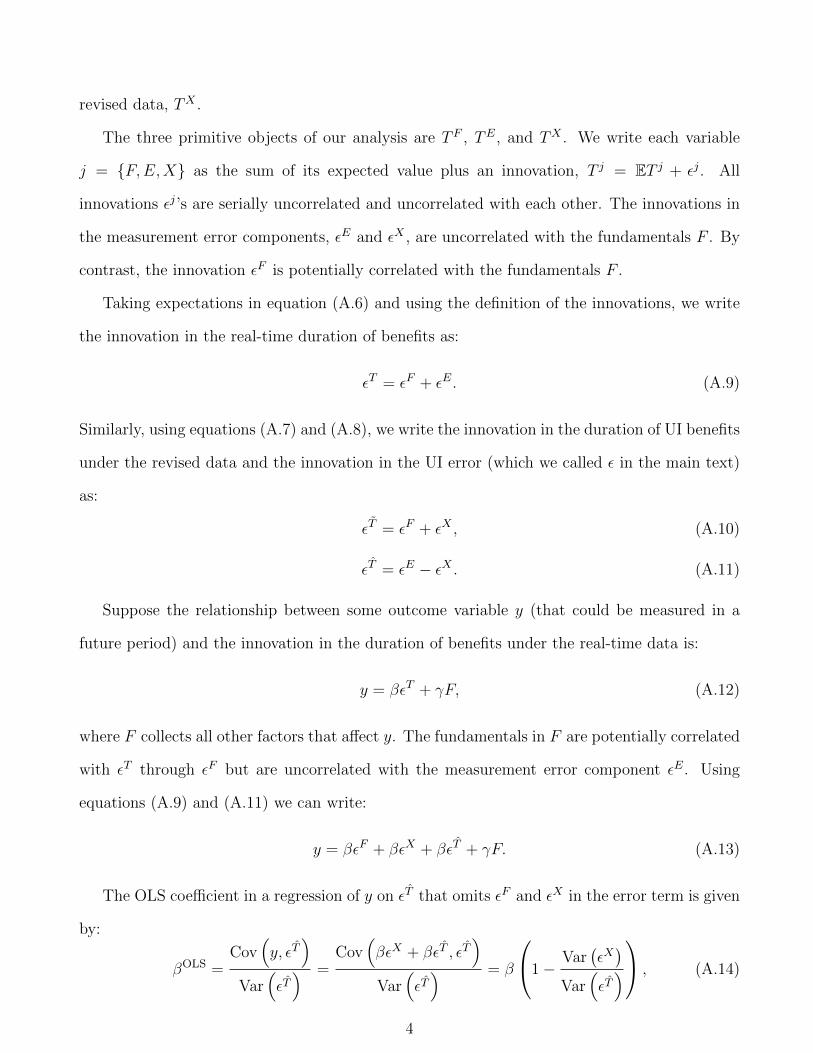
revised data, TX .

The three primitive objects of our analysis are TF , TE, and TX . We write each variable

j = {F,E,X} as the sum of its expected value plus an innovation, T j = ET j + εj. All

innovations εj’s are serially uncorrelated and uncorrelated with each other. The innovations in

the measurement error components, εE and εX , are uncorrelated with the fundamentals F . By

contrast, the innovation εF is potentially correlated with the fundamentals F .

Taking expectations in equation (A.6) and using the definition of the innovations, we write

the innovation in the real-time duration of benefits as:

εT = εF + εE. (A.9)

Similarly, using equations (A.7) and (A.8), we write the innovation in the duration of UI benefits

under the revised data and the innovation in the UI error (which we called ε in the main text)

as:

εT = εF + εX , (A.10)

εT = εE − εX . (A.11)

Suppose the relationship between some outcome variable y (that could be measured in a

future period) and the innovation in the duration of benefits under the real-time data is:

y = βεT + γF, (A.12)

where F collects all other factors that affect y. The fundamentals in F are potentially correlated

with εT through εF but are uncorrelated with the measurement error component εE. Using

equations (A.9) and (A.11) we can write:

y = βεF + βεX + βεT + γF. (A.13)

The OLS coefficient in a regression of y on εT that omits εF and εX in the error term is given

by:

βOLS =Cov

(y, εT

)Var

(εT) =

Cov(βεX + βεT , εT

)Var

(εT) = β

1−Var

(εX)

Var(εT) , (A.14)

4

where the second equality uses equation (A.13) and the fact that Cov(F, εT

)= Cov

(εF , εT

)=

0, and the third equality uses the fact that Cov(εX , εT

)= Cov

(εX , εE − εX

)= −Var

(εX). If

the revised data measure the true fundamentals without any error up to a constant, Var(εX)

=

0, then the OLS estimator is unbiased βOLS = β. The attenuation bias is increasing in the

variance of the measurement error in the revised data relative to the variance of the UI error,

Var(εX)/Var

(εT)

.

We now show that attenuation bias in our estimates is too small to affect our main conclusions

under the plausible assumption that revised data do not deteriorate the quality of measurement

of true fundamentals. We say that the revised data are a (weakly) better measure of the true

fundamentals than the real-time data if the measurement error in the revised data has a (weakly)

lower variance:

Var(εX)≤ Var

(εE). (A.15)

The assumption that the revised data contain less measurement error than the real-time data

places an upper bound on the attenuation bias. From equation (A.11), we see that Var(εT)

=

Var(εX)

+ Var(εE)

and, therefore, under equation (A.15) less than 50 percent of the variance

of εT is attributed to εX :

Var(εX)

Var(εT) ≤ 0.5. (A.16)

We estimate in the data an upper bound of βOLS = 0.02. Using the upper bound of the bias

Var(εX)/Var

(εT)

= 0.50, the true coefficient could be as large as β = 0.04. Using a standard

error of 0.02, this β is still 4.5 standard errors below the 0.15 level that would rationalize a large

effect of extended benefits on unemployment during the Great Recession.

This calculation is very conservative because it assumes that revisions do not improve mea-

surement and uses the upper bound of our estimates of β. In Section 3.4 we provided ev-

idence that revisions are informative about actual spending patterns and beliefs. This im-

plies that Var(εX)/Var

(εT)

is likely to be smaller than 0.5. Indeed, we find in the data

that there is smaller variance of outcomes in the revised data and, consistent with our as-

5

sumption that Var(εX)≤ Var

(εE), that Var

(εT)< Var

(εT). If we apply, for example,

Var(εX)/Var

(εT)

= 0.25 to our maximum estimate of βOLS = 0.02, we obtain that the true

coefficient is β < 0.03. More in general, the more informative is the revised data for the true

fundamentals, the lower is Var(εX)/Var

(εT)

and the smaller is the attenuation bias.

C Model Appendix

In this appendix we present additional results from the model. In Figures A.1, A.2, and A.3,

we present the impulses of the fraction of unemployed receiving UI, the log opportunity cost,

and log vacancies to a one-month increase in the UI error innovation. In Figures A.4 and A.5

we depict the path of productivity and separations shocks underlying the experiment depicted

in Figure 8 in the main text. In each figure, the left panel corresponds to the high b model and

the right panel corresponds to the low b model.

In Figure A.6 we illustrate the Regression Discontinuity (RD) framework using model-

generated data. The point we wish to make is that, under very persistent shocks, a pure RD

framework is not able to detect significant effects of UI benefit extensions on macroeconomic

outcomes despite the existence of such effects. For this figure, we continue to use the same

parameters as in the high b model of Table 10 except that we increase the persistence of log

productivity to ρ = 0.98. We also adjust the volatility of the productivity shocks to σ = 0.004

so that the model generates the same volatility of log productivity as the baseline high b model

in the main text. We then simulate the model for a large number of periods.

The right panel of Figure A.6 shows the relationship between ut+1 in the vertical axis and ut

in the horizontal axis generated by the model. The left panel of the figure shows the relationship

between ut+2 and ut. The plotted lines denote third-order polynomials fitted on model-generated

data left and right of the cutoffs denoted with vertical lines. As we see in the figure, there is no

significant discontinuity around the points in which the duration of benefits increases sharply.

When shocks are very persistent, forward-looking agents in an economy that starts just below

the cutoff expect benefit extensions in the future. Therefore, equilibrium outcomes are not

6

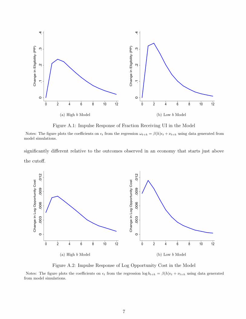
0.1

.2.3

.4

Ch

an

ge

in E

ligib

ility

(P

P)

0 2 4 6 8 10 12

(a) High b Model

0.1

.2.3

.4

Ch

an

ge

in E

ligib

ility

(P

P)

0 2 4 6 8 10 12

(b) Low b Model

Figure A.1: Impulse Response of Fraction Receiving UI in the Model

Notes: The figure plots the coefficients on εt from the regression ωt+h = β(h)εt + νt+h using data generated frommodel simulations.

significantly different relative to the outcomes observed in an economy that starts just above

the cutoff.

0.0

03

.00

6.0

09

.01

2

Ch

an

ge

in L

og

Op

po

rtu

nity

Co

st

0 2 4 6 8 10 12

(a) High b Model

0.0

03

.00

6.0

09

.01

2

Ch

an

ge

in L

og

Op

po

rtu

nity

Co

st

0 2 4 6 8 10 12

(b) Low b Model

Figure A.2: Impulse Response of Log Opportunity Cost in the Model

Notes: The figure plots the coefficients on εt from the regression log bt+h = β(h)εt + νt+h using data generatedfrom model simulations.

7

-.0

4-.

02

0

Ch

an

ge

in L

og

Va

can

cie

s

0 2 4 6 8 10 12

(a) High b Model

-.0

4-.

02

0

Ch

an

ge

in L

og

Va

can

cie

s

0 2 4 6 8 10 12

(b) Low b Model

Figure A.3: Impulse Response of Log Vacancies in the Model

Notes: The figure plots the coefficients on εt from the regression log vt+h = β(h)εt + νt+h using data generatedfrom model simulations.

-.0

5-.

04

-.0

3-.

02

-.0

10

Lo

g P

rod

uct

ivity

0 10 22 34 46 58 70

With Benefit Extensions No Benefit Extensions

(a) High b Model

-.0

5-.

04

-.0

3-.

02

-.0

10

Lo

g P

rod

uct

ivity

0 10 22 34 46 58 70

With Benefit Extensions No Benefit Extensions

(b) Low b Model

Figure A.4: Productivity Path in the Model

Notes: The figure plots the path of productivity used to generate the simulation in Figure 8.

8

.03

.04

.05

.06

Se

pa

ratio

n R

ate

0 10 22 34 46 58 70

With Benefit Extensions No Benefit Extensions

(a) High b Model

.03

.04

.05

.06

Se

pa

ratio

n R

ate

0 10 22 34 46 58 70

With Benefit Extensions No Benefit Extensions

(b) Low b Model

Figure A.5: Separations in the Model

Notes: The figure plots the path of the separation rate used to generate the simulation in Figure 8.

.04

.06

.08

.1.1

2

ut+

1

.04 .055 .065 .08 .09 .105ut

(a) Unemployment Rate in t+ 1

.04

.06

.08

.1.1

2

ut+

2

.04 .055 .065 .08 .09 .105ut

(b) Unemployment Rate in t+ 2

Figure A.6: Regression Discontinuity in Model-Generated Data

Notes: The figure plots the relationship between ut and ut+1 (left panel) and ut+2 (right panel) generated fromsimulated data.

9

Tab

leA

.1:

Exte

nded

Ben

efit

and

Em

erge

ncy

Com

pen

sati

onP

rogr

ams,

1996

-201

5

Pro

gram

Tie

rW

eeks

Per

iod

Tri

gger

sE

B1

1309

/25/

1982

-.IU

R≥

5,IU

R≥

1.2*

[(IU

R(y

ear

ago)

+IU

R(2

year

sag

o))/

2]O

RIU

R≥

6O

RT

UR≥

6.5

and

TU

R≥

1.1∗

max{T

UR

(yea

rag

o),T

UR

(2ye

ars

ago)}

EB

27

03/0

7/19

93-.

TU

R≥

8an

dT

UR≥

1.1∗

max{T

UR

(yea

rag

o),T

UR

(2ye

ars

ago)}

EB

1,2

n.a

.12

/17/

2010

-12/

31/2

013

Rep

lace

wit

hm

ax{T

UR

(yea

rag

o),T

UR

(2ye

ars

ago)

,TU

R(3

year

sag

o)}

inE

BT

ier

1T

rigg

er3

and

EB

Tie

r2

Tri

gger

1T

EU

C1

1303

/09/

2002

-12/

31/2

003

Ava

ilab

lein

all

stat

esT

EU

C2

1303

/09/

2002

-12/

31/2

003

Eligi

ble

for

EB

orw

ould

be

elig

ible

ifE

BT

ier

1T

rigg

er1

cuto

fffo

rIU

Rw

ere

4in

stea

dof

5E

UC

113

06/3

0/20

08-1

1/20

/200

8A

vailab

lein

all

stat

esE

UC

120

11/2

1/20

08-0

9/01

/201

2A

vailab

lein

all

stat

esE

UC

114

09/0

2/20

12-1

2/31

/201

3A

vailab

lein

all

stat

esE

UC

213

11/2

1/20

08-1

1/05

/200

9E

ligi

ble

for

EB

OR

IUR≥

4O

RT

UR≥

6E

UC

214

11/0

6/20

09-0

5/31

/201

2A

vailab

lein

all

stat

esE

UC

214

06/0

1/20

12-1

2/31

/201

3T

UR≥

6E

UC

313

11/0

6/20

09-0

5/31

/201

2IU

R≥

4O

RT

UR≥

6E

UC

313

06/0

1/20

12-0

9/01

/201

2IU

R≥

4O

RT

UR≥

7E

UC

39

09/0

2/20

12-1

2/31

/201

3IU

R≥

4O

RT

UR≥

7E

UC

46

11/0

6/20

09-0

5/31

/201

2IU

R≥

6O

RT

UR≥

8.5

EU

C4

606

/01/

2012

-09/

01/2

012

IUR≥

6O

RT

UR≥

9E

UC

410

09/0

2/20

12-1

2/31

/201

3IU

R≥

6O

RT

UR≥

9

Not

es:

Tri

gger

sw

ritt

enin

ital

ics

are

opti

onal

.IU

Ris

the

aver

age

of

the

insu

red

un

emp

loym

ent

rate

inth

eth

irte

enw

eeks

end

ing

two

wee

ks

bef

ore

the

wee

kof

the

trig

ger

not

ice.

TU

Ris

the

aver

age

ofth

eto

tal

un

emp

loym

ent

rate

inth

eth

ree

month

sen

din

gw

ith

the

last

month

of

data

rep

ort

edas

of

the

thir

dF

rid

ayb

efor

eth

eS

un

day

star

tin

gth

ew

eek

ofth

etr

igger

noti

ce.

All

pro

gra

ms

an

dti

ers

ob

eya

thir

teen

wee

kru

lew

her

eby

on

cetr

igger

edon

ati

era

stat

ere

mai

ns

onth

atti

erfo

rat

leas

tth

irte

enw

eeks

(barr

ing

any

chan

ges

inla

w),

an

don

cetr

igger

edoff

ati

erth

est

ate

rem

ain

soff

for

at

least

thir

teen

wee

ks.

Th

eti

me

per

iods

rep

orte

dex

clu

de

ph

ase-

outs

.E

BT

ier

1T

rigger

3b

ecam

eop

erati

on

al

on

03/07/1993.

Au

thori

zati

on

of

the

TE

UC

pro

gra

ms

lap

sed

tem

por

aril

yb

etw

een

01/0

1/20

03an

d01/

07/2

003.

Au

thori

zati

on

of

the

EU

Cp

rogra

ms

lap

sed

tem

pora

rily

bet

wee

n04/04/2010

an

d04/14/2010,

bet

wee

n05

/30/

2010

and

07/2

1/20

10,

and

bet

wee

n11

/28/

2010

an

d12/16/2010.

Bet

wee

n02/22/2012

an

d05/31/20

12

indiv

idu

als

cou

ldre

ceiv

eu

pto

16

wee

ks

of

EU

CT

ier

4b

enefi

tsif

thei

rst

ate

was

not

inan

EB

per

iod

.T

he

main

sou

rce

for

this

tab

leis

Dep

art

men

tof

Lab

or

(2015).

10