The Macroeconomic Effects of Government Asset Purchases:Evidence from Postwar US Housing Credit Policy∗

Andrew Fieldhouse

Cornell University

Karel Mertens†

FRB Dallas, NBER, CEPR

Morten O. Ravn

University College London, CEPR, Centre for Macroeconomics

July 24, 2017

Abstract

We document the portfolio activity of federal housing agencies and provide evidence on its impact onmortgage markets and the economy. Through a narrative analysis, we identify historical policy changesleading to expansions or contractions in agency mortgage holdings. Based on those regulatory events thatwe classify as unrelated to short-run cyclical or credit market shocks, we find that an increase in mortgagepurchases by the agencies boosts mortgage lending, in particular refinancing, and lowers mortgage rates.Agency purchases influence prices in other asset markets, stimulate residential investment and expandhomeownership. Using information in GSE stock prices to construct an alternative instrument for agencypurchasing activity yields very similar results as our benchmark narrative identification approach.

Keywords: Credit Policy, Monetary Policy, Mortgage Credit, Residential Investment, Government-Sponsored EntreprisesJEL Classification: E44, E52, N22, R38, G28

∗We are grateful to the Department of Housing and Urban Development as well as Shane Sherlund for providing data, and toparticipants at various seminars for useful comments. Karel Mertens acknowledges the hospitality of the Economics Departmentat Colombia University where parts of the research were conducted. Financial support from the ADEMU (H2020, No. 649396)project and from the ESRC Centre for Macroeconomics is gratefully acknowledged. The views in this paper are those of theauthors and do not necessarily reflect the views of the Federal Reserve Bank of Dallas or the Federal Reserve System.

†Contact: Federal Reserve Bank of Dallas, karel.mertens@dal.frb.org, tel: +(214) 922-6000

1 Introduction

The residential mortgage market in the United States is one of the largest capital markets in the world and by

far the dominant source of credit for American households. The mortgage market finances housing, which

is a key component of both household wealth and aggregate spending, see e.g. Leamer (2007). Many ac-

counts of the causes and propagating factors of the 2007/08 financial crisis assign an important role to a

boom and bust in the availability of mortgage credit.1 The US mortgage market is also subject to heavy

government involvement through various federal agencies, including the housing government-sponsored en-

terprises (GSEs). In the decades preceding the 2007/08 crisis, the various agencies collectively accumulated

a large share of the total outstanding US mortgage debt on their balance sheets. In this paper, we investigate

whether agency portfolio purchases of mortgage assets influence the availability and cost of housing credit,

and whether there are spillovers to other debt markets and economic activity more broadly.

While the history of agency activity offers a rich source of variation to study the effects of government

asset purchases, it also presents a number of challenges. The largest agencies, Fannie Mae and Freddie Mac,

have been privately owned for much of their existence and therefore carry responsibilities to stock owners as

well as to their public missions of providing “stability” and “ongoing assistance” in mortgage markets. Both

profit and public objectives cause these agencies to systematically and rapidly respond to market conditions,

such that changes in their mortgage purchasing activity reflect changes in housing credit demand and many

other influences. Some of the correlation between agency balance sheets on the one hand and credit growth

or mortgage rates on the other is therefore likely to reflect reverse causality.

We propose two different strategies to isolate changes in agency purchasing activity free of confounding in-

fluences. Our first and principal strategy is to focus on historical credit policy interventions affecting agency

mortgage holdings, in the spirit of the approaches in Romer and Romer (1989, 2010) and Ramey (2011) to

studying monetary and fiscal policy. Based on a narrative analysis of the regulatory history of the housing

agencies, we identify and quantify significant policy events affecting agency purchases. These include ad-

justments to capital requirements, portfolio caps, or statutory borrowing authority, direct appropriations and

1 See e.g. Mian and Sufi (2009), Justiniano, Primiceri, and Tambalotti (2014), or Di Maggio and Kermani (2016).

1

capital injections by the Treasury, or changes to the pool of mortgages eligible for agency purchase, such as

changes in conforming loan limits or authorizations to enter new mortgage market segments.

Credit policy changes are often reactions to cyclical conditions in mortgage and housing markets, the recent

crisis being a prime example. However, many interventions are motivated by other longer run objectives

such as increasing homeownership. Based on an extensive analysis of historical sources, we classify each

significant credit policy change as motivated by either cyclical considerations or by other non-cyclical ob-

jectives.2 This results in an indicator summarizing the non-cyclically motivated policy events, which we

use as an instrumental variable in regressions of a variety of outcome variables on measures of agency pur-

chasing activity. Similar to the approach in Ramey and Zubairy (2016) to estimating government spending

multipliers, we estimate the cumulative effects of an increase in agency purchases on mortgage credit and

originations, as well as impulse responses to news shocks about future agency purchasing activity.

Our second and complementary identification approach is based on instrumenting measures of agency pur-

chasing activity with orthogonalized innovations in Fannie and Freddie excess stock returns. This alternative

strategy is analogous to Fisher and Peters (2010), who use excess return innovations in major US defense

stocks as a measure of news shocks to military spending. Passmore (2005) estimates that the advantages

granted by federal housing credit policy account for much of the market value and portfolio size of Fannie

and Freddie. We show that news about policy interventions affecting GSE balance sheets is reflected in their

stock market valuation. Positioned last in a causal ordering behind credit aggregates, interest rates, and other

macro variables, we find that residual variation in Fannie and Freddie excess stock returns predicts agency

mortgage purchases. This motivates us to use this residual variation as an alternative instrumental variable

to estimate the response of credit aggregates to shocks to agency mortgage purchases.

It is not clear ex ante that government purchases of mortgage assets have meaningful effects on the cost

and availability of housing credit. If financial market frictions are relatively unimportant, an increase in

agency purchases may have little impact on the volume of mortgage credit, and simply lead to crowding out

2The full narrative analysis is in a companion background paper, Fieldhouse and Mertens (2017), available at http://www.nber.org/papers/w23165.

2

of private holdings. If such frictions are instead pervasive, mortgage market policies may on the other hand

be very important for the provision of credit to residential borrowers. Based on our methodology, we find

that agency purchases indeed lead to statistically significant expansions in mortgage credit. Our estimates

indicate that each additional dollar in agency mortgage purchases leads to a 3 to 4 dollar cumulative increase

in mortgage originations over the course of three to four years, and a net expansion in the stock of mortgage

debt of around one dollar. The rise in originations is largely driven by an increase in refinancing activity, but

is also followed by a greater volume of originations financing home purchases. The expansionary effects on

housing credit are accompanied by temporary reductions in mortgage interest rates, which fall by 10 to 15 ba-

sis points for more than a year following an increase in agency purchases of one percent of trend originations.

Agency purchases also affect prices in other asset markets. We estimate that the 10-year Treasury rate

and the 3-month T-bill rate both decline when the agencies increase their purchases of mortgages. A key

policy objective behind President Hoover’s introduction of housing credit policies in the 1930s was to stim-

ulate the construction sector, while another recurrent motivation has been to promote homeownership. We

find evidence that supports these roles of the agencies in that new housing starts and homeownership rates

rise following an increase in agency mortgage purchases. We also find some evidence that agency mortgage

purchases increase house prices and stimulate private sector consumption. There is no clear evidence of any

significant impact on the unemployment rate or personal income.

Perhaps our most surprising finding concerns the relationship between housing credit and monetary poli-

cies. We show that the narratively identified housing credit policy shocks have forecasting power for the

residual shock component of the Romer and Romer (2004) decomposition of funds rate target changes,

while the reverse is not true. Instead, we find that cyclically motivated housing credit policy changes lean

against the wind of contractionary monetary disturbances. Housing credit policy shocks have larger effects

on refinancing originations than interest rate shocks, and influence homeownership independent of short-

term interest rates. The quantitative effects of housing credit policy and conventional monetary shocks are

very similar along many other dimensions. These findings suggest that both may share similar transmission

channels, and that the interplay between monetary and credit policy deserves more attention.

3

2 Mortgage Purchases as Credit Policy in the United States

The US government intervenes in the mortgage market in many ways. We focus attention on the federal

involvement in purchasing residential mortgages. The first significant use of this type of policy dates back

to the Great Depression. The sharp and sustained downturn in credit markets motivated Congress to create

the Home Owners’ Loan Corporation in 1933. Financed by bonds, the Corporation purchased delinquent

mortgages from lenders and refinanced these mortgages into fully amortizing fixed-rate loans with long

maturities to lower monthly payments for distressed mortgagors. In 1938, Congress created Fannie Mae

to support a secondary market for government-guaranteed mortgages. Fannie’s authority to acquire mort-

gage debt was increased greatly after WWII to support the construction sector and promote homeownership

among veterans. The late 1960s saw the creation of Ginnie Mae to provide continued support the market

for government-guaranteed mortgages. In 1970, Fannie Mae obtained permission to enter the conventional

market, i.e. the market for loans not directly guaranteed or insured by the government, and the newly created

Freddie Mac joined Fannie Mae in developing a nationwide secondary market for conventional mortgages.

Over time, the agencies have played an increasingly active role. The two largest GSEs, Fannie and Freddie,

acquire mortgages through advance commitments to buy loans from mortgage lenders, which are delivered

once the loans are originated in the primary market.3 Until the late 1960s, the purchases by Fannie were

financed predominantly by borrowing from the Treasury. Afterwards, as quasi-private entities, Fannie and

Freddie have financed these purchases with a mix of private capital and debt issued in capital markets. A

third financing option is the issuance of mortgage pools, i.e. mortgage-backed securities (MBS). Securitiza-

tion was brought to the conventional market by Freddie Mac in the early 1970s, and took off in the 1980s

when it was also adopted by Fannie Mae. Mortgage securitization has consistently been GSE-dominated,

perhaps with the brief exception of the 2004-2006 private-label securitization boom. In the process of pack-

aging whole mortgages into securities, the agencies also assume the credit risk in return for guarantee fees.

From the early 1990s onwards, the agencies increasingly retained their own and acquired each other’s MBS,

as opposed to selling them to private investors.

3Another major housing GSE is the Federal Home Loan Bank System, chartered during the Depression to provide wholesaleliquidity to member mortgage lending institutions. We use the term ‘GSE’ to refer to Fannie and Freddie.

4

Figure 1 illustrates the evolution of agency involvement in the residential mortgage market over time. The

upper left panel shows the stock of total residential mortgage debt both as a ratio of GDP and as ratio of

total residential wealth. The upper right panel shows the total annualized volume of residential mortgage

originations as a ratio of GDP and as a fraction of outstanding mortgage debt. The lower panels of Figure 1

provide measures of agency market shares, constructed by consolidating data on holdings and net purchases

of whole loans and MBS as reported on the agencies’ balance sheet and activity statements. The left panel

shows the fraction of mortgage debt owned by Fannie, Freddie, and Ginnie as well as all other federal agen-

cies with mortgage holdings, such as the Federal Home Loan Banks and the Federal Reserve.4 The lower

right panel show the flows of net mortgage purchases by the agencies as a percentage of total originations.

The blue line shows the net portfolio purchases. To distinguish these portfolio purchases clearly from those

for securitization, the figure also shows in red the combined issuance of MBS by the agencies.5

The post-WWII period witnessed a marked expansion in mortgage debt, rising from around 10 percent

of GDP at the end of WWII to more than 80 percent by 2008, before steadily declining in the wake of the

2007/08 financial crisis. Originations of new mortgages are volatile, procyclical, and average around 20

percent of outstanding debt at an annualized rate.6 By any measure, the government agencies have over time

become large players in the mortgage market. Between 1980 and 2006, total purchases in the secondary

market by Fannie and Freddie alone average around 40 to 50 percent of originations. The majority of these

acquisitions were packaged in MBS and sold off to private investors. The portfolio purchases, comprising

whole loans retained for the portfolio as well as net acquisitions of MBS, have averaged 7 percent of origi-

nations between 1967 and 1990, and about 15 percent between 1990 and 2006. At the peak in 2004, almost

a quarter of all residential mortgage debt resided on the balance sheet of a federal agency, with roughly 20

percent owned by Fannie and Freddie alone. In early September 2008, Fannie and Freddie were taken into

conservatorship and were required to gradually wind-down their balance sheets by two-thirds. The Federal

4 Other agencies include the Home Owners’ Loan Corporation, Treasury, Veterans Administration, Federal Housing Adminis-tration, Federal Farmers Home Administration, Resolution Trust Corporation, Federal Deposit Insurance Corporation, and PublicHousing Administration. We do not include mortgages in government pension funds. See the data appendix for sources.

5 Because purchases may include loans originated in prior periods, the market shares may occasionally exceed 100 percent.6Net additions to the stock of mortgage debt are considerably smaller than originations since both existing home sales as well

as refinancing transactions typically lead to minor net changes in mortgage debt.

5

Reserve subsequently pursued several rounds of large-scale purchases of agency MBS under its quantitative

easing (QE) programs, and its current holdings amount to roughly 15 percent of total mortgage debt out-

standing. For readers wishing more information about the institutional history of the housing agencies, the

appendix provides more background.

The focus of this paper is on the portfolio purchases of the housing agencies, shown in blue in the lower

right panel in Figure 1. Prior to the Fed’s QE programs, Fannie and Freddie accounted for the bulk of

agency mortgage acquisitions. Even as privately owned corporations, Fannie and Freddie have been key

agents of federal housing policy and differ from traditional financial intermediaries in a number of important

ways. First, they have always maintained authorization to borrow from the Treasury. While this autho-

rization was limited and never formally exercised, it sufficed to create the widely held belief that the US

government would never allow a GSE to default. This perception, eventually justified by the government

takeover of Fannie and Freddie in 2008, meant that interest rates on agency bonds have typically been close

to Treasury rates. Second, agency debt is eligible for open market operations by the Fed. In the 1960s and

1970s the Fed made significant purchases of agency debt, see Haltum and Sharp (2014), and again so under

the QE programs. Third, the prudential supervision of the GSEs is separate from private banks and, prior to

2008, resided within the Department of Housing and Urban Development (HUD).7 Regulatory oversight of

the GSEs was traditionally light compared to that of private banks, and the GSEs generally enjoyed much

less stringent capital and reporting requirements. For instance, despite being publicly listed companies, Fan-

nie and Freddie were exempt from filing with the Security and Exchange Commission until the early 2000s.

Finally, for much of their existence, the GSEs have also benefitted from various preferential tax treatments.

In exchange for the privileges granted by federal law, the GSEs face a number of restrictions and obliga-

tions. Fannie and Freddie cannot originate loans in the primary market and are not allowed to diversify

portfolio holdings much beyond mortgage assets. Their purchases are limited to conforming mortgages that

must meet certain underwriting standards, and the principal on the loans cannot exceed a maximum amount,

known as the conforming loan limit. The authority for adjusting the limit and other loan characteristics that

7Since 2008, the regulatory authority lies with the Federal Housing Finance Agency, an independent federal agency.

6

determine what mortgages are conforming has generally lied with Congress and the HUD Secretary. In 1980

the conforming loan limit became indexed to a house price index maintained by Freddie Mac. Since then

typically around 80 percent of mortgages have been conforming.8 Finally, the GSEs are expected to balance

stock owner interests with certain public policy objectives, including the stabilization and enhancement of

mortgage markets, as well as assistance with the provision of credit to lower-income households.

3 Related Literature

There are relatively few attempts at identifying the dynamic effects of agency purchases on mortgage credit,

residential investment or homeownership. An early literature estimates reduced form models of credit and

housing markets to assess the impact of GSE activity in the 1970s, e.g. Arcelus and Meltzer (1973), Meltzer

(1974), Hendershott and Villani (1977, 1980), Jaffee and Rosen (1978), and Kaufman (1985). Although no

clear consensus emerges from this early work, Smith, Rosen, and Fallis (1988) conclude that an additional

dollar in government lending increases mortgage debt by 25 to 35 cents after three to four quarters. Arcelus

and Meltzer (1973) and Meltzer (1974), however, argue there is no effect on residential investment or home

purchases, while Jaffee and Rosen (1978) and Hendershott and Villani (1977, 1980) find a positive impact

of agency activity on home construction.

Starting with Hendershott and Shilling (1989), a number of studies document significant interest rate spreads

between conforming and jumbo loans, which suggests that the GSEs affect the cost of mortgage credit.

Hendershott and Shilling (1989) attribute this result to a credit supply channel operating through agency

securitization. A number of studies investigate the time series relationship between GSE activity and credit

costs. Naranjo and Toevs (2002), for instance, find a negative long-run relationship between GSE purchases

and mortgage rates, while Gonzalez-Rivera (2001) finds only a negative short-run relationship.9 Lehnert,

8In response to the financial crisis, the limit was increased substantially for the financing of homes in urban areas, whichfurther expanded the pool of mortgage debt eligible for GSE purchase.

9Naranjo and Toevs (2002), who use vector error-correction (VEC) and GARCH (generalized autoregressive conditional het-eroskedastic) models and monthly time series data from 1986 to 1998, find that both GSE purchases and securitization reduceconforming mortgage spreads and volatility, while documenting some spill over to reductions in non-conforming loans, whichthey attribute to investor substitution effects. Gonzalez-Rivera (2001), who uses VEC models and monthly data from 1994 to1999, finds a negative short-run relationship of GSE purchases responding to widening secondary mortgage market spreads, andsome evidence of a pass through from secondary to primary mortgage rates from agency purchases.

7

Passmore, and Sherlund (2008) study the impact of GSE activities on primary and secondary market mort-

gage spreads using both generalized impulse response analysis and causal orderings in VAR models. Based

on monthly data from 1993 to 2005, these authors find little evidence that higher GSE purchases impact

mortgage spreads, which is consistent with the Meltzer view that credit market interventions are neutral. In

a May 2005 speech, Federal Reserve Chairman Alan Greenspan conveys a similar view of the role of the

GSEs’ portfolio activities, stating that “Fannie’s and Freddie’s purchases... with their market-subsidized

debt do not contribute usefully to mortgage market liquidity, to the enhancement of capital markets in the

United States, or to the lowering of mortgage rates for homeowners” (Greenspan, 2005).

In this paper, we contribute new evidence against the Greenspan-Meltzer view that agency mortgage pur-

chase have little effect on the cost and availability of mortgage credit. Our approach is similar in spirit to

Lehnert et al. (2008), but adopts novel and arguably better identification strategies to control for the endo-

geneity of agency purchases. We also study a much longer time frame than any of the earlier papers, and we

estimate the effects on both credit aggregates and mortgage rates. Moreover, our dynamic regressions allow

us to study many other variables of interest, including housing starts, home prices, homeownership rates,

cyclical indicators, and various other interest rates and credit spreads.

Our paper is related to the many analyses of the large-scale MBS purchases by the Federal Reserve un-

der the QE programs. To isolate the effects of these purchases, the literature typically restricts attention to

high frequency financial data, and most studies conclude that the MBS purchases lowered secondary market

mortgage yields on impact, see e.g. Gagnon et al. (2011), Krishnamurthy and Vissing-Jørgensen (2011), Pa-

trabansh, Doerner, and Asin (2014), and Hancock and Passmore (2011, 2015).10 Exploiting cross-sectional

variation, a few recent studies also uncover evidence that is suggestive of a positive impact on mortgage

lending. Di Maggio, Kermani, and Palmer (2016), for instance, find that, after the first QE intervention,

originations of mortgages qualifying for inclusion in securities eligible for purchase by the Fed increased

substantially more than those of non-qualifying mortgages. No such differential effects are evident after

the second QE intervention, which did not include MBS purchases. Darmouni and Rodnyansky (2016)

10Stroebel and Taylor (2012) instead find no effects of the MBS purchases under QE1.

8

find that banks with larger mortgage positions increased lending relative to banks with smaller positions,

and Chakraborty, Goldstein, and MacKinlay (2016) show that banks with MBS exposure increased their

mortgage origination share relative to other banks. By studying a longer history of housing credit policy

interventions, we are able to circumvent some key limitations of the event studies of the Fed’s large-scale

MBS purchases. Our approach permits an analysis beyond the very short-run response of financial variables,

and unlike the cross-sectional studies, provides direct evidence on aggregate rather than relative effects.

Our study also fits in a broader empirical literature that aims to identify credit supply shocks and esti-

mate their aggregate effects. Peek, Rosengren, and Tootell (2003), for instance, use bank health indicators

as proxies for loan supply shocks and find substantial effects on inventory investment and other aggregates.

Gilchrist and Zakrajsek (2012) look at innovations in corporate bond spreads after removing cyclical default

premia, and demonstrate their strong predictive content for macroeconomic fluctuations. Bassett, Chosak,

Driscoll and Zakrajsek (2014) study residual variation in survey measures of bank lending standards and find

an impact on economic activity. Mian, Sufi, and Verner (2017) use variation in the timing of bank branching

deregulation in the 1980s to construct differential state-level credit supply shocks, and find that these shocks

impact household borrowing and employment. Both our narrative policy indicator and the GSE excess return

shocks can similarly be viewed as proxies for credit supply shocks in the mortgage market.

Many existing theories of financial frictions can explain the non-neutrality of agency mortgage purchases.

Krishnamurthy and Vissing-Jørgensen (2011) and Di Maggio et al. (2016), among others, discuss a variety of

potential transmission channels associated with the MBS purchases under the QE programs. Many of these

channels have similar implications for mortgage purchases by the GSEs. Through the portfolio rebalancing

channel, for instance, private investors bid up the price of mortgages when rebalancing assets towards some

desired composition of mortgages and agency liabilities. For the GSEs, the latter are not reserves, but debt

instruments that closely substitute for Treasuries in terms of liquidity and (perceived) safety.11 Depending

on the level of segmentation in financial markets, rebalancing effects may spill over to other asset markets,

in which case yields on mortgage substitutes—particularly other types of long-term debt—may fall as well.

11This difference may be less important if the Federal Reserve simultaneously acquires agency debt.

9

Agency mortgage purchases also matter when private mortgage lenders face capital constraints because of

regulations or binding incentive constraints, for instance as in the theoretical models of Gertler and Kiyotaki

(2010) or Curdia and Woodford (2011). Because the GSEs are more highly leveraged than private lenders,

aggregate lending capacity increases with agency market share. Agency purchases that drive up the price of

mortgages may additionally improve the net worth position of private mortgage lenders, while the exchange

of mortgages for agency debt lowers their risk-weighted leverage ratios. Increased agency activity in the

secondary mortgage market may also reduce liquidity premia. Our findings support a role for credit supply

channels in determining household debt, homeownership, and residential investment, but it is beyond the

scope of this paper to isolate precisely which of these channels may be more important.

4 Identifying Causal Effects of Agency Mortgage Purchases

4.1 Endogeneity Problems

To assess the impact of agency portfolio purchases, one might be tempted to simply correlate measures of

agency activity, such as those in Figure 1, with credit and other macroeconomic aggregates. This would,

however, ignore various endogeneity problems. For one, the agencies respond to changes in market condi-

tions. To maintain market share, for instance, the GSEs vary purchases with the supply of mortgages into the

secondary market, which in turn depends on fluctuations in the housing market and the economy. A different

endogeneity concern is that agency purchases typically expand relative to the mortgage market when credit

is tight and/or conditions in the housing market are deteriorating. This was evidently the case during the

latest financial crisis through the actions of the Fed and Treasury, but is also true of earlier episodes.

Figure 2 shows the average real levels of agency and private holdings of mortgage debt over the course

of business and credit cycles since the mid-1950s. The left panel of Figure 2 shows the average real levels of

agency and privately held mortgage debt centered around NBER business cycle peaks. On average, growth

in agency holdings is high relative to growth in private holdings prior to a business cycle peak. The growth

in private mortgage holdings slows down just prior to the peak and remains low for a prolonged period after

the start of a recession. The pace of growth of agency holdings, in contrast, remains roughly unchanged for

10

at least two years after the beginning of an economic downturn.

The right panel of Figure 2 shows the average real levels of mortgage holdings centered around the peak

of credit cycles, defined as the quarter preceding the start of credit crisis episodes based on the datings in

Eckstein and Sinai (1986) and subsequent updates.12 Agency and private holdings grow at roughly similar

rates prior to a credit crunch. Growth in private holdings of mortgage debt slows markedly following the

start of a credit crisis. In contrast, growth in agency holdings accelerates at the onset of a credit crunch and

remains elevated for about ten quarters, before flattening toward the pre-crunch trend.

The evidence thus indicates that agencies tend to increase their share of the market in cyclical downturns and

credit crunches. These countercyclical purchase dynamics are robust to omitting the 2007/08 crisis and the

Federal Reserve’s interventions. There are a number of reasons why the agencies jointly maintain or expand

purchases during cyclical downturns. A public mission to provide stability to mortgage markets is mandated

in the GSEs’ statutory charters. Credit crises also offer particularly profitable opportunities for the GSEs be-

cause their lending spreads widen relative to private intermediaries, due to countercyclical mortgage spreads

and the implicit guarantee provided by the US government. Finally, the federal government often undertakes

deliberate regulatory or legislative actions to further enable agency expansions during downturns. The fact

that agency purchases tend to accelerate when mortgage spreads are elevated and/or credit is tight induces a

negative relationship with mortgage credit aggregates. This negative association needs to be accounted for

in order to determine the causal effects of agency mortgage purchases.

4.2 Narrative Analysis of Policy Changes Affecting Agency Mortgage Holdings

Our principal strategy to control for reverse causality in the relationship between agency mortgage purchases

and credit conditions is to use a narrative identification approach involving major regulatory events impact-

ing agency mortgage holdings. By focusing on policy interventions by the federal government, we exclude

variation in purchase activity resulting from the agencies’ regular response to market developments. Be-

12The dating of pre-1986 credit crunches is from Eckstein and Sinai (1986). The dating of post-1986 crunches is based onOwens and Schreft (1993) for the 1990 commercial real estate crunch, Lehnert, Passmore, and Sherlund (2008) for the 1998Russian default/LTCM crisis, and Bordo and Haubrich (2010) for the 2007/08 financial crisis.

11

cause policymakers themselves often respond to conditions in mortgage and housing markets, we exclude

interventions with short-run stabilization motives as the primary objective. The end result of our narrative

analysis is a record of housing credit policy events that we use as an instrumental variable for agency pur-

chase activity. Here, we summarize the methodology of the narrative analysis, and describe the resulting

policy indicators. A companion background paper, Fieldhouse and Mertens (2017), provides the full nar-

rative analysis of credit policy events, including explanations of relevant findings for each policy event and

extensive documentation that allows verification of our analysis.

4.2.1 Overview of Methodology

The development of the narrative instrumental variable follows five steps: Identifying significant policy

changes affecting agency portfolios; quantifying their ex ante projected impact on agency holdings; pin-

pointing the timing of when the policies became publicly known; classifying each policy change as either

cyclically or non-cyclically motivated; and restricting the sample for consistent use as an instrument for

agency purchasing activity. Next, we describe the procedures used in each of these steps. Table 1 provides

an overview of the historical primary sources used in the narrative analysis.

I. Identifying Significant Policy Changes Policy changes affecting agency purchases and mortgages hold-

ings have historically been directed by a range of policymakers, notably Congress, the President and the

Cabinet, particularly the Secretaries of the Treasury and HUD, various regulatory agencies in the executive

branch, and the Federal Reserve. The relevant regulatory institutions were disbanded and reinvented several

times over the decades, and as a result there is no single consistent source tracking the history of housing

credit policy. Instead, a wide range of sources is required for identifying and analyzing policy changes.

Policy actions generally originate from one of three sources: enacted legislative changes, regulatory policy

changes published in the Federal Register or as other binding agreements with regulators, and macroeco-

nomic stabilization policies managed by the Federal Reserve or Treasury. We restrict attention to significant

policy actions, meaning actions that would either be expected to directly impact agencies’ permissible vol-

ume of net purchases and retained portfolio holdings, or else considerably expand the pool of eligible mort-

12

gages an agency was authorized or required to purchase. Interventions determined at the legislative level

include adjusting statutory leverage ratios, capital requirements, and conforming loan limits, provision of

working capital, mandatory retirements of public stock, and direct appropriations or borrowing authority for

purchases, among others. Regulatory policy actions include setting permissible debt-to-capital ratios, impos-

ing capital surcharges in excess of statutory capital requirements, capping portfolio size or growth, setting

affordable housing goals, and authorizing entrance to new segments of the mortgage market. Macroeco-

nomic stabilization actions include the Fannie and Freddie conservatorship agreement in September 2008,

subsequent amendments to these agreements, and the large-scale MBS purchase programs conducted by the

Federal Reserve and Treasury since 2008.

We use the comprehensive Congressional Research Service report “A Chronology of Housing Legislation

and Selected Executive Actions, 1892-2003” (CRS, 2004) as a starting point for identifying significant pol-

icy changes, particularly pertinent public laws. This legislative history is cross-referenced with the Congres-

sional Quarterly Almanac’s Housing and Development tracker. We additionally search appendices of the

Budget of the United States Government for information about policy changes affecting Ginnie Mae during

relevant years, cross-referenced with HUD appropriations bills and related reports of the House and Sen-

ate Appropriations Committees. After identifying public laws affecting the agencies, we use the ProQuest

Congressional Publications Database to collect the legislative text of those enacted laws, related committee

reports and Congressional hearing transcripts, and any preceding House and Senate versions of the final

bill.13 We then analyze relevant sections of these primary sources to confirm these laws’ material impact on

mortgage holdings and better understand the nature of the policy changes.

Legislative actions often set in motion the drafting of new regulatory rules. Identified significant legislative

events are the starting point for a directed search of the related regulatory changes in HeinOnline’s Federal

Register Library. We also obtain information from the GSEs’ annual reports about significant regulatory

changes, as well as from 10-K filings in more recent years. We additionally used sections of the Economic

13The ProQuest Congressional Publications Database provides a comprehensive compilation of all public laws, committeereports, and hearings. Public laws and related legislative actions since 1973 are available from Congress.gov, a project of theLibrary of Congress, along with committee reports since 1995. Most older public laws are available through LegisWorks Statutesat Large Project. Most hearing transcripts are digitally available since 1985 from the US Government Publishing Office.

13

Report of the President and Annual Report of the Board of Governors of the Federal Reserve, as well as the

various reports by regulators to collect information about regulatory rulings. We use newspapers, financial

newswires, and mortgage industry newsletters to help direct the search for information about the rulings in

the Federal Register, particularly the Wall Street Journal, American Banker, and National Mortgage News.14

Final rules published in the Federal Register almost always include a detailed background and overview of

the initial proposed rule, public comments received, and subsequent modifications.

Using these procedures, we are confident that we have identified the overwhelming majority of significant

policy events. The main concern is developing a policy indicator that is correlated with underlying regula-

tory shocks to agency purchasing activity. The larger the number of significant policy events identified, the

higher the relevance of the instrument.

II. Quantification To be included, we require that primary sources either explicitly cite projections of the

policy change’s impact, or contain information that can be used to quantify the impact. We describe here

our general approach, and show later that the resulting projections align closely with the ex post estimated

balance sheet impact.

For each policy change, we use contemporaneous sources to obtain an ex ante estimate of the projected

impact on the agencies’ capacity to purchase mortgages, measured in annualized billions of dollars. If a

baseline is needed for quantifying a policy change, say for Fannie’s regulatory capital when its debt-to-

capital ratio is increased, we use the most recent data publicly available prior to the policy change. We

use ex ante balance sheet data on regulatory capital, liabilities, and/or assets in conjunction with standing

leverage or capitalization requirements to estimate the impact of related changes, such as increases in per-

missible leverage ratios. Similarly, public capital injections are quantified as a multiple of one more than the

prevailing leverage ratio, to capture the potential increase in assets supported by related debt issues plus the

working capital itself. Direct appropriations are straightforward to quantify, at most requiring a pro-rata an-

nualization adjustment based on relevant implementation lags. To quantify potential impacts of discretionary14This is done by Factiva and LexisNexis Academic searches of key words related to the regulatory policy change, in search

windows around the vicinity of the event. After roughly pinpointing the publication date of a rule, we search the Federal Registerfor the rule itself, and then work backwards to initial rulings.

14

conforming loan limit changes, we rely on estimates from Congressional committee reports accompanying

legislation. Such reports typically cite the extent to which a large conforming loan limit increase would

restore a GSE’s real purchase activity. We quantify the impact of such adjustments as the difference between

annualized purchase volumes immediately preceding the policy change and the home price index-adjusted

purchase volume of the benchmark year being restored. For relatively large, open-ended changes, such as

leverage ratio increases, potential effects on mortgage holdings are annualized using a two-year rule, which

assumes half of the full potential impact would be realized within the first year of taking effect.

For other policies that are inherently harder to quantify, such as authorizations for program expansions into

new mortgage market segments, we search for ex ante estimates of projected impacts on purchasing activity

from committee reports, market analysts, regulators, or agency executives. We do not include policies that

would not have been expected to impose or alleviate binding constraints on agency activity. For instance,

when adjustments to leverage ratios or affordable housing goals are viewed as non-binding by most accounts

and this appears consistent with the agencies’ balance sheet and purchase behavior, we do not consider the

policy change significant. We also exclude any laws or regulations that merely extend prior authorizations,

and for certain authorizations affecting Ginnie Mae, we use a current policy baseline as opposed to a current

law baseline for scoring annual funding changes.

When estimating the quantitative aspects of the policies, we rely on information released by the Congres-

sional Budget Office, Government Accountability Office, Treasury Department, and Congressional Research

Service that contain detailed analyses of policy changes, background information, and/or balance sheet data

for the agencies in question, see Table 1. We also use information from the annual or periodic reports of the

agencies and regulators, particularly regarding balance sheet data, and from appropriations bills and budget

appendices for certain policies affecting Ginnie Mae. Committee report language occasionally cites pro-

jected effects of a pending policy change, and we also use the financial press and industry newsletters to

search for projections of the impact of policies that are difficult to quantify.

15

III. Timing At the operational level, the agencies sell commitments to purchase conforming mortgages

from primary market lenders, which may then be exercised by the mortgagee up to an expiration date. Con-

sequently, actual agency purchases tend to lag behind the issuance of commitments to purchase mortgages

from primary market originators. Together with the usual policy implementation lags, the policy events are

therefore best thought of as news shocks about agency mortgage purchases. We date each policy interven-

tion to the month in which we estimate that it became publicly anticipated, rather than the month in which

it was formally announced or took effect. We show in the next section that this timing approach is roughly

consistent with the observed movements in consolidated agency mortgage holdings.

The ProQuest Congressional Publications Database, HeinOnline’s Federal Register Library, the CQ Al-

manac, and financial press are the primary sources used for documenting pertinent news surrounding policy

changes and the implementation dates. For regulatory changes, we use the month in which proposed rules

were first published in the Federal Register or reported in the press. We date legislative changes when the

provision including the policy change was agreed upon in the House, Senate, or conference version of a

bill, rather than upon subsequent enactment. For Fannie and Freddie, we additionally check the timing by

cross-referencing policy announcements with GSE stock price movements and the financial press, as often

policy news is priced into GSE shares.

IV. Classification by Motivation The classification of the policy events distinguishes between interven-

tions that are guided by prevailing business cycle and financial conditions, and those that are plausibly free

of such contemporaneous influences. Our instrument for agency mortgage purchases only includes the latter

to avoid bias due to the systematic relaxation of policies during periods of stress in mortgage or housing

markets. The classification is based on identifying the primary motivations underlying each of the pol-

icy interventions. To make this classification, we parse historical documents, paying particular attention

to the rationales invoked by policymakers and the press, the nature of the legislative vehicles or regulatory

processes, the relation to known periods of economic and financial stress, and the time horizon of policy

objectives.

16

The principal data sources for identifying policy motives include Congressional committee reports and hear-

ings, Presidential speeches and signing statements, the Budget of the US Government, Economic Report of

the President, Federal Reserve Bulletin, Annual Report of the Board of Governors of the Federal Reserve,

CQ Almanac, and the financial press (see Table 1). For legislated policies, the accompanying reports of the

Senate Committee on Banking, Housing and Urban Affairs and the House Financial Services Committee

typically detail congressional intent and any pertinent economic context. Major housing policy laws are

also usually accompanied by a Presidential signing statement explaining the bill’s motivation, context, and

intended impact. Budget appendices and/or committee reports accompanying appropriations bills usually

explain the impetus for certain policy changes affecting Ginnie Mae. Final rules published in the Federal

Register also almost always include a detailed background and history, shedding light on regulators’ motives.

Based on these sources, we classify the policy changes as either cyclically motivated or non-cyclically mo-

tivated. Interventions classified as cyclically motivated tend to emphasize short-term outcomes, such as

boosting housing starts in a recession. Legislative vehicles for such policy actions tend to be quickly drafted

and enacted, with a relatively concise legislative history and narrow focus. Policymakers are typically quite

explicit about cyclical concerns and objectives, overwhelmingly so when policies are implemented in close

proximity to recessions or credit crunches. Language we search for in committee reports and signing state-

ments as strong evidence of cyclical motivations include “emergency, crisis, recession, credit shortage, credit

crunch, housing starts, employment, construction, downturn, depressed, stimulus, boost”, etc. Policies en-

acted during or near a recession or credit crunch are held to a particularly high bar for being classified as

non-cyclical, but are not automatically classified as cyclically motivated.

Interventions motivated by social policy, budgetary, or other more ideological objectives are classified as

unrelated to the business or financial cycle, provided the various historical sources do not at the same time

indicate significant short-term economic or financial market concerns. Political rather than economic context

shapes the development of these interventions, such as an administration’s emphasis on expanding affordable

homeownership opportunities to lower-income households, concerns regarding the structural budget deficit,

or ideological hostility toward the GSEs. It is often hard to establish a single rationale for the non-cyclical ac-

17

tions, which can be motivated by a mix of objectives. For our purposes, however, a more precise distinction

between these objectives is not essential. Language we search for as indicative of non-cyclical motivations

include “long-term, farsighted, comprehensive, low-income, affordable housing, American Dream, home-

ownership, budget deficit, reduce borrowing, off-budget, privatize,” etc. Legislative actions classified as

non-cyclical emphasize longer-term outcomes, such as increasing homeownership rates. Legislative vehi-

cles for such interventions tend to be slower-moving bills, particularly deliberate overhauls of housing policy

with a lengthy legislative history; the National Housing Acts, Housing and Urban Development Acts, and

Housing and Community Development Acts of various years tend to meet this description, being slowly

crafted and negotiated between the House, Senate, and White House, and focusing on broad, long-term

objectives for housing policy, such as urban revitalization or access to affordable housing for various con-

stituencies. New regulatory rules set in motion by such bills also tend to be classified as non-cyclical, such

as HUD setting new affordable housing goals for the GSEs. Occasionally, interventions are prompted by

specific events that we view as unrelated to the cycle, such as the regulatory actions taken in the aftermath

of accounting scandals at Fannie and Freddie in 2003-2004.

V. Sample Restrictions Occasionally a law or public rule sets in place changes in purchase authorizations

or balance sheet restrictions to take effect only multiple years after announcement. To obtain a good indicator

for news about pending purchase behavior, we exclude changes with very long implementation delays and

focus on interventions taking effect within nine months of their news being made public. We also restrict

attention to policy events after January 1967. This choice is made to select a period of relative institutional

stability, as it roughly coincides with the creation of Ginnie and Freddie, the emergence of a nationwide

secondary market for conventional mortgages, and the beginning of the ascendancy of the privatized GSE

era. This starting point is also in part determined by the availability of time series used in the empirical

analysis. We focus exclusively on the mortgage portfolio activity of Fannie, Freddie, and Ginnie, ignoring

less significant government entities for which monthly data is not easily available. We also include purchases

by the Federal Reserve and Treasury in the recent financial crisis, but in most of the analysis in Sections 5

and 6 the sample is truncated at December 2006 to deliberately exclude the financial crisis and the Fannie and

Freddie conservatorship period. As shown in Figure 1, the three housing agencies that we analyze account

18

for the large majority of government agency mortgage holdings between 1967 and 2006.

4.2.2 The Narrative Measures of Policy Changes

Table 2 lists the policy events resulting from the narrative analysis. Each intervention is described by the

agencies affected, by its annualized projected impact (in billions of US dollars), timing, and motivation. The

monthly sample contains 45 months with interventions in the post 1967 sample (there are 52 interventions in

total but some occur within the same month). Out of these, 28 are classified as cyclically motivated, leaving

19 distinct non-cyclically motivated policy events. In the sample that excludes interventions after December

2006, there are 15 cyclically and 17 non-cyclically motivated policy events.

Figure 3 depicts the interventions as a percentage of the average annualized level of originations in the

preceding 12 months. The left (right) panel shows the non-cyclical (cyclical) policy indicator. For refer-

ence, each figure also shows credit crisis episodes in grey. The cyclically motivated interventions almost all

occur during credit crunches or recessions, while those not motivated by cyclical concerns appear unrelated

to the cycle. The largest interventions are those introduced since the start of the 2007/08 financial crisis,

which are mostly classified as cyclical.15 The only post-2006 events that we consider non-cyclical are the

removal of Fannie and Freddie portfolio caps in February 2008, which was contingent on the timely filing

of financial reports after the accounting scandals, and a 2012 Treasury decision to accelerate the mandated

decline in portfolio caps under the GSE conservatorship agreements. Relative to average originations, the

three largest non-cyclical changes are the October 1977 combination of a conforming loan limit increase

and the expansion of the Brooke-Cranston Tandem program, an increase in Fannie’s debt-to-capital limit in

December 1982, and the tightening of Fannie’s capital requirements in September 2004 in the wake of the

accounting scandals. We refer to Fieldhouse and Mertens (2017) for a detailed discussion of all policy events.

Do the policy changes that we have narratively identified lead to actual changes in agency purchases and

retained mortgage portfolios? To investigate this, it is important to take into account the potentially sig-

nificant delays between the policy events and their impact on the agency portfolios. Recall that agencies

15These include the Fed and Treasury MBS programs from late 2008 onwards, but also the loosening of capital requirementsand portfolio caps for Fannie and Freddie and the introduction of ‘jumbo’ conforming loan limits in 2008.

19

initially make advance commitments to buy loans from mortgage providers and subsequently effectuate

these as loans are originated in the primary market. We regress three activity indicators, net mortgage pur-

chase commitments made by the agencies, the actual net purchases of mortgages, and the stock of agency

mortgage holdings, on the indicator for non-cyclical policy events mt :

yt = α+36

∑j=−l

β jmt− j +ut (1)

We use monthly observations from January 1967 to December 2014 in log first differences of current dol-

lars. Because monthly commitment and purchase flows are relatively volatile, we run the regressions for a

36 month backward moving average of these two variables. The event indicator mt is the non-cyclically mo-

tivated narrative measure scaled by the average level of agency mortgage holdings over the prior 12 months.

All regressions include the current value of mt as well as three years of lags. For each activity measure, we

estimate two versions of (1), one in which we set l = 0 and one in which l = 12. The second version includes

a full year of leads of mt , which allows us to verify the plausibility of our timing of the interventions. Figure

4 shows the estimated dynamics of the agency activity measures around the policy events, obtained as the

sum of the slope coefficients β j over various horizons, together with 95 percent Newey and West (1987)

confidence bands.

The policy change indicator strongly predicts significant changes in agency purchase commitments (left

panel) which pick up at date 0 and peak at a 3 to 4 percent higher level roughly two years out. Actual

purchases (middle panel) follow a very similar trajectory as commitments, but with a lag of a few months,

demonstrating that the policy changes act as news shocks for actual purchases. The right panel shows that

the higher pace of mortgage purchases is followed by a persistent and statistically significant increase in the

agencies’ retained portfolio.

The specifications allowing a lead response to the events suggest that our indicator accurately captures the

timing of the change in purchasing activity. It is also encouraging that the size of the estimated response of

agency mortgage holdings converges to around one percent within 24 months of the policy event, which is

20

consistent with our scoring of the projected impact of the policy changes.

5 The Cumulative Effects of Agency Mortgage Purchases on Mortgage Credit

We estimate the cumulative impact of agency mortgage purchases on credit aggregates by using the non-

cyclically motivated policy changes as an instrument for agency purchasing activity. As shown in Figure 1,

the growth in mortgage debt over our sample period has on average exceeded growth in GDP, while agency

holdings have increased at an even faster pace. Because of these differential trends, expressing the impact

on credit aggregates and other variables in terms of elasticities can be misleading.16 To address these issues,

we run local projections-IV regressions similar to those used by Ramey and Zubairy (2016) to estimate cu-

mulative government spending multipliers.

Our results are based on local projections for horizon h and outcome variable yt of the form

yt+h − yt−1

Xt= αh + γh

∑hj=0 pt+ j

Xt+ϕh(L)Zt−1 +ut+h (2)

where pt is either the volume of commitments or actual purchases by the agencies in month t. Both yt and

pt are expressed in constant dollars using the core PCE price index. For every horizon h, the change in yt as

well as the cumulative change in commitments or purchases pt is expressed as a ratio of Xt , a deterministic

trend in real personal income obtained by fitting a third degree polynomial of time to the log of personal in-

come deflated by the core PCE price index.17 For stock variables, the dependent variable is the change in the

stock between t −1 and period t +h, scaled by Xt . For credit flow measures, we construct yt by cumulating

the flows ft such that yt+h − yt−1 = ∑hj=0 ft+ j.

Each regression includes a full year of monthly lags of a number of control variables Zt , such that ϕh(L)

is a lag polynomial of order 11. The controls include variables with predictive content for the dependent

variables, and always include lagged values of yt/Xt (or ft/Xt for flow variables), as well as lags of agency

16Both the news aspect and the scaling issues also occur in other contexts, in particular in the measurement of the effects offiscal policy interventions, see for instance Ramey (2011), Mertens and Ravn (2012), and Ramey and Zubairy (2016).

17The results do not differ meaningfully when we use polynomials of different order. In online appendix A.1, we also showthat the results are robust to using a trend in mortgage originations instead of personal income.

21

net purchases and commitments as a ratio of Xt . In addition Zt contains lagged growth rates of the core PCE

price index, a nominal house price index and total mortgage debt, the log level of real mortgage originations,

housing starts, and lags of several interest rate variables: the 3-month T-bill rate, the 10-year Treasury rate,

the conventional mortgage interest rate, and the BAA-AAA corporate bond spread. Finally, we add lags of

two cyclical indicators: the unemployment rate and the growth rate of real personal income. All growth rates

are quarter-over-quarter. The data appendix provides full details on the sources and construction of the time

series. In online appendix A.1, we discuss results for a number of alternative control (sub)sets.

The coefficient γh in (2) measures the multiplier associated with an additional dollar in commitments or

purchases made between period t and t + h. This multiplier is the total cumulative dollar change in yt be-

tween period t and t +h. We estimate γh by two-stage least squares (2SLS) using the dollar impact estimates

of the non-cyclically motivated policy events reported in Table 2, deflated by the core PCE price index and

expressed as a ratio of Xt , as the instrument. Our baseline estimates use an effective sample of 480 monthly

observations, starting in January 1967.18 In online appendix A.1, we look at different sample periods.

The central identifying restriction is exogeneity of the instrument, which requires that the residuals in (2) and

the narrative measure are uncorrelated. To the extent that the lagged controls are informationally equivalent

to all relevant impulses to the dependent variables occurring prior to time t, the regression residuals corre-

spond to their horizon h forecast errors. The latter depend only on unpredictable shocks occurring between

period t and t + h. Our instrument is based on the projected impact of policy events constructed from ex

ante information. These estimates should therefore be uncorrelated with shocks occurring after time t. The

identifying restriction then boils down to the assumption of orthogonality between the instrument and all

shocks in month t other than the one associated with the policy event itself. If the control set does not fully

capture all impulses prior to date t−1, then the exogeneity requirement is stricter and the instrument must be

uncorrelated with the history of relevant impulses to the left hand side variables. The omission of the cycli-

cally motivated events aims at dropping policy actions that may be correlated with all other time t shocks.

18With local projections, every successive horizon h = 0,1,2... requires a separate regression with h leads of observationsbeyond the end point of the sample, see Jorda (2005) for a discussion. For h > 0, we add the required observations beyondDecember 2006 such that the number of observations remains constant at T = 480 for every h.

22

Our narrative classification retains the non-cyclically motivated events for which correlation with contem-

poraneous shocks is unlikely, while the lagged controls provide additional insurance that the confounding

effects of any remaining correlations with prior shocks are eliminated, see also Ramey (2016).

5.1 First-Stage Diagnostics

We first assess the strength of our narrative instrument. The left panel of Figure 5 shows the Newey and

West (1987) robust F-statistics on the excluded instrument in the first-stage regressions for horizons h = 0 to

h = 60, which are of the form

∑hj=0 pt+ j

Xt= αh + γh

mt

Xt+ ϕh(L)Zt−1 + ut+h (3)

where mt is the non-cyclical narrative policy indicator expressed in real dollars. The figure shows the F-

statistics when using either cumulative commitments or purchases as the measure of agency activity pt .

The results indicate that the narrative measure is a reasonably strong instrument for agency purchasing

activity for horizons between 4 to 48 months after the policy events, with robust F-test statistics exceeding

or close to 10. The F-statistics are low for very short horizons, which is natural given the implementation

lags and our timing according to the arrival of news about impending regulatory changes. Beyond horizons

of 48 months, the F-statistics fall to lower levels, which is also not surprising as other influences on agency

purchases accumulate with the forecast horizon. Given these results we restrict attention to the 4- to 48-

month horizon. The F-statistics are very similar when we instrument for either purchases or commitments.

The right panel of Figure 5 depicts IV estimates of the dollar change in agency purchases for every dol-

lar of commitments issued over the various time horizons based on the regressions in (2) using cumulative

agency purchases as the outcome variable and cumulative commitments as the independent variable. The

fine lines denote 95 percent Newey and West (1987) confidence intervals. Because of the time delays as-

sociated with secondary market transactions, the pass-through from commitments to purchases is high but

smaller than unity for shorter horizons. After about one year the relationship becomes one-for-one with very

23

narrow confidence intervals. The interpretation of the credit multiplier estimates presented next therefore

depends somewhat on the denominator used, but only for horizons of less than one year. At longer horizons,

there is essentially no difference between using commitments or purchases as the agency action measure.

5.2 Cumulative Credit Multipliers

According to the Meltzer-Greenspan view, the portfolio activities of the agencies have no meaningful im-

pact on housing or household debt. Without credit market imperfections, the ownership of mortgage debt is

irrelevant. Any change in agency mortgage holdings has no impact on total mortgage debt, but leads instead

to perfect crowding out of private holdings. If, on the other hand, there are frictions impeding on the pri-

vate flow of credit to residential borrowers, agency activity may not be neutral for the volume of mortgage

lending. We now examine whether agency mortgage purchases indeed impact housing credit, and test the

neutrality hypothesis using the local projections in (2) and the narrative policy instrument.

Figure 6 shows the impact of an increase in either agency commitments or purchases, together with the

95 percent Newey and West (1987) confidence bands. There is a marked difference between the short and

long-run effects. In the short run, the results are consistent with neutrality: The upper left panel shows that

a dollar purchased increases agency mortgage holdings initially by almost a dollar. The short-run effect of

a dollar increase in commitments on agency holdings is lower at around 60 cents, which is expected given

the time delay between commitments and purchases. The right panel shows that private holdings decline

initially by roughly the same amount as the increase in agency holdings, although the confidence bands are

wide.19 The middle panels in Figure 6 show that as the dollar in mortgage debt changes from private to

agency ownership, there are initially no significant changes in originations or mortgage debt.

Over longer horizons, however, there is clear evidence against the notion that agency purchases are neu-

tral for mortgage credit. The cumulative impact on total mortgage originations increases with the horizon

and becomes statistically significant after 6 months. Over the course of 3 years and beyond, there is a

19This almost surely reflects the fact that our measure of private holdings is partially based on interpolation of quarterly data.Private holdings are measured by subtracting agency holdings from total mortgage debt. Total mortgage debt is constructed usingmonthly data on originations and an interpolation of implied quarterly repayment rates. See the data appendix for more detail.

24

cumulative increase in originations of 3 dollars or more for every dollar purchased by the agencies. The

estimated long-run multipliers for total originations are highly statistically significant and nearly identical

for commitments and purchases. The point estimates for the impact on the stock of mortgage debt at shorter

horizons are roughly in line with the range reported in Smith, Rosen, and Fallis (1988). The increase in

mortgage debt becomes statistically significant after three to four years and in the longer run reaches a level

of around one dollar. As the time horizon grows, the increase in agency holdings slowly dissipates toward

levels expected before the expansion. Similarly, the negative impact on the level of private mortgage hold-

ings vanishes over time and eventually turns into an increase, although not one that is statistically significant.

The results in the middle row of Figure 6 imply that agency portfolio expansions lead to a substantial rise in

mortgage lending activity. Originations take place when borrowers refinance, purchase an existing home, or

purchase a new home. Unless there are changes in house prices or homeownership, the first two transactions

typically lead only to small net changes in mortgage debt because a similar amount of mortgage debt is

repaid. Since the increase in originations is a multiple of the net change in debt, it is likely driven mostly by

a rise in transactions of the first two types, with new home purchases playing a more important role beyond

horizons of two years. The bottom row of Figure 6 distinguishes between refinancing originations in the

left panel, and home purchase originations in the right.20 Refinancing originations indeed respond faster

and by a substantially larger amount than purchase originations. Refinancing originations see a statistically

significant increase beyond 6 months, and within 3 years are higher by roughly 3 dollars per dollar of agency

purchases. Home purchase originations rise more slowly and are statistically significantly higher after 18

months, increasing by nearly one dollar within 4 years. The rise in purchase originations occurs somewhat

faster than the rise in total mortgage debt, suggesting that existing home sales respond before new home

sales. The longer-run cumulative change in purchase originations is comparable to the increase in mortgage

debt, which suggests a positive impact on residential construction. In the impulse response analysis below,

we indeed find evidence for an increase in housing starts. We also document positive effects on homeown-

ership rates and, although less clearly, on home prices, both of which also contribute to the rise in mortgage

20Data prior to 1990 is approximated using the refinancing share of S&Ls, see data appendix. Unfortunately, we were unableto find data distinguishing between originations for new and existing home sales with a sufficient time span.

25

debt. The bulk of the effect on originations is nevertheless due to refinancing.21

Given the procyclicality of mortgage originations, the large positive effect on originations makes it unlikely

that the estimates are severely contaminated by the countercyclical actions of the agencies over the sample.

The decrease in private holdings and the delayed effect on originations also suggest that the estimates are not

merely picking up increased supply of mortgages to the secondary market, as would occur if private lenders

simply passed on newly originated loans to the agencies; if this were the case, originations would rise before

or roughly simultaneously with agency purchases and without a decline in private holdings. It is precisely

in this direction that the results change when we instead estimate γh in (2) by ordinary least-squares (OLS).

To illustrate this, Figure 7 compares the OLS and 2SLS responses of mortgage originations. Regardless of

whether the baseline or full set of controls is included, the OLS estimates suggest that the bulk of the increase

in originations occurs within a few months. Given the decision lags and time delays associated with making

new mortgage loans, the delayed and gradual rise in originations that appears after instrumentation is much

more consistent with a causal interpretation. The comparison in Figure 7 is generally informative about

the endogeneity concerns in practice. Systematic GSE expansions during times of high primary mortgage

demand or high private sector credit supply would lead to an upward bias using OLS, while the stabilizing

actions of the agencies lead to a downward bias. Since the OLS estimates exceed the 2SLS estimates for

horizons up to 2 years, the former appears the dominant practical concern in our sample.22

6 Impulse Response Analysis of News Shocks to Agency Purchases

To evaluate the effects of agency purchases on residential investment and homeownership, as well as analyze

the response of interest rates and other macro aggregates, in this section we conduct an impulse response

analysis of shocks to agency mortgage purchases. Given the gradual and anticipated nature of agency balance

sheet expansions, our goal is to identify the response to shocks to expectations of future agency purchasing

21This is consistent with Di Maggio et al. (2016), who document an increase in refinancing activity by 170% during the Fed’sfirst QE program.

22In online appendix A.1, we elaborate on the role of instrumenting, and we discuss additional results on agency securitization.We also verify robustness in several dimensions, such as the choice of scaling variable Xt , the sample choice, the set of controls,as well as the exclusion of specific policy events in the narrative instrument. The expansionary effects of agency purchases onmortgage credit are shown to be robust to many details of the analysis.

26

activity. We adopt a local projections approach and use the narrative instrument for identification. We also

present results for an alternative instrumentation strategy that exploits information in GSE stock prices.

6.1 Empirical Specification with the Narrative Instrument

For a given monthly outcome variable yt , we estimate the response at horizon h based on

yt+h − yt−1 = αh +δh

(128×

∑7j=0 pt+ j

Xt

)+ϕh(L)Zt−1 +ut+h (4)

The right hand side variable of interest measures annualized agency commitments made over an 8 month

period, expressed as a ratio of Xt , a long-run trend in annualized originations. The latter is obtained by fitting

a third degree polynomial of time to the log of real originations obtained using the core PCE price index as

the deflator. The control variables Zt−1 are the same as in equation (2) estimating dollar cumulative effects.

When an outcome variable is not included in the benchmark control set, we always add 12 monthly lags of

that variable as additional controls (in growth rates for trending variables and in levels for other variables).

The regression in (4) estimates the month h ≥ 0 response to a time 0 news shock to agency purchases.

Expected agency purchases are proxied by agency commitments made over the next 8 months. We choose

an 8 month horizon to measure expected future commitments because at this horizon the robust F-statistic

associated with the narrative instrument in the first-stage regression is the largest, and equals 11.68. The

results are very similar for somewhat shorter or longer horizons. To address endogeneity, we use the indi-

cator of non-cyclical policy events, deflated by the core PCE price index and scaled by trend originations

Xt , as the instrument. The IV estimates of δh in (4) can be interpreted as the response associated with a one

percentage point increase in the agency flow market share that becomes anticipated h periods before. For

perspective, the average market share in terms of portfolio purchases was approximately 7 percent between

1967 and 1990, and about 15 percent between 1990 and 2006, see Figure 1.

27

6.2 Empirical Specification with the GSE Excess Returns Instrument

Although our narrative instrument is a good predictor of agency purchasing activity, it is based on relatively

few policy events. It is therefore always possible that our findings are driven by the small sample size. To

gain confidence that this is not the case, as well as address other potential concerns with the narrative identi-

fication method, we also pursue an alternative approach inspired by Fisher and Peters (2010). These authors

interpret innovations in excess stock returns of major defense contractors as news shocks about future mil-

itary spending. Fisher and Peters (2010) obtain these innovations by ordering the excess returns last in a

recursively identified structural vector autoregressive system. The recursive scheme assumes that none of

the macro aggregates included in the analysis are affected on impact by the news shock, while excess stock

returns react contemporaneously to all macroeconomic shocks. We follow a similar strategy to identify the

response to news shocks to agency purchases.23

Passmore (2005) estimates that 44 percent to 89 percent of Fannie and Freddie’s stock market value is

derived from their special GSE status, and that the GSEs would hold far fewer mortgages in portfolio and

have higher capital ratios if they were purely private. Any news about changes in the policies guiding the

GSEs’ portfolios business and leverage is thus likely to affect their market value. To construct an alternative

measure of news of agency purchasing activity, we identify innovations in the excess return of GSE stock

based on similar recursivity assumptions as Fisher and Peters (2010). To implement these assumptions, we

estimate the response at horizon h through the following regression:

yt+h − yt−1 = αh +δh

(128×

∑7j=0 pt+ j

Xt

)+ζhWt +ϕh(L)Zt−1 +ut+h (5)

Relative to (4), this specification adds the contemporaneous controls Wt , which includes the interest rate

variables (3-month T-bill, 10-year Treasury, the conventional rate, BAA spread), the log of real originations,

the log changes in mortgage debt, real house prices, the core PCE price index and personal income, the log

of housing starts, and the unemployment rate. When we rotate in another variable, we also include it in Wt .

One other modification relative to (4) is that the log of the GSE stock price-to-S&P 500 ratio is added to Zt .

23Different from Fisher and Peters (2010), we use local projections-IV. Online appendix A.5 shows that the SVAR approachyields similar results.

28

The response coefficient δh in (5) is estimated using 2SLS, where the first stage is a regression of the log

change in the GSE stock price-to-S&P 500 ratio on Wt and Zt−1. This specification imposes that shocks to

expected agency purchases have no contemporaneous impact on the variables in Wt . The instrument used

in the 2SLS estimation of (5) is therefore the monthly innovation in the GSE excess stock return, orthogo-

nalized to the monthly innovations in the variables in Wt . By assumption, other endogenous influences on

GSE excess returns, such as shocks to household demand for mortgages, are eliminated by allowing excess

returns to respond contemporaneously to mortgage credit, interest rates, prices, and the cyclical indicators.

Figure 8 plots the standardized cumulative sum of these innovations, together with the non-cyclical narrative

indicator for reference. The GSE excess returns shocks are followed by statistically significant increases in

agency purchasing activity. The F-statistic for the GSE excess returns instrument is the highest for agency

commitments at a horizon of 5 months, and equals 8.55.24 To provide further evidence that GSE stock prices

reflect changes in agency purchasing activity, Figure 9 plots the response of the GSE stock price-to-S&P 500

ratio to a one pp. increase in the expected future agency market share, measured by agency commitments

as a ratio of trend originations. This response is estimated by (4) using the narrative policy indicator as the

instrument, and reveals a clear relative increase in GSE stock prices that is statistically significant at horizons

of 4 to 12 months. Fieldhouse and Mertens (2017) also provide narrative evidence that announcements of

policy changes affecting Fannie and Freddie are generally associated with adjustments in their stock prices.

Because the GSE excess returns instrument contains monthly observations, it potentially contains more

information about variation in agency purchases than the narrative policy indicator.25 Our narrative indica-

tor contains, for instance, little information for the 1990s because of the scarcity of quantifiable and binding

regulatory changes. However, this period witnessed a rapid expansion of GSE balance sheets and may be

particularly important for learning the effects of agency purchases. As is well known, however, equity prices

24For simplicity, we keep the horizon for cumulating commitments in equation (5) at 8 months, the same as in equation (4).The value of the first-stage robust F-statistic for this horizon is 7.68. Changing the horizon for cumulating commitments inspecification (5) to 5 months does not lead to any meaningful changes in the results.

25Assuming the GSE excess returns shocks contain all of the information about agency purchase shocks, it becomes possible toestimate the variance contribution of these shocks to any endogenous variables of interest. In online appendix A.5, we do this inthe context of an SVAR model.

29

are volatile, and the GSE excess return shocks are, on the other hand, also relatively noisy. While the GSE ex-

cess returns shocks clearly have predictive power for agency commitment activity, the first-stage F-statistics

are somewhat lower than for the narrative instrument. Another caveat is that the GSE excess return shocks

may also pick up unanticipated variation in the scale of the GSEs’ securitization business. Nevertheless, we

view this identification strategy as a useful alternative to the narrative approach. The next sections show that

both instruments generally lead to very similar impulse response estimates.

6.3 Effects on Mortgage Credit and Interest Rates

Figure 10 displays the responses of mortgage credit and interest rates to news about higher future purchases.

Each of the panels shows the point estimates and confidence bands for the first 24 months after an increase in

anticipated agency purchases by one percentage point of trend originations. The responses in blue are based

on the narrative instrument, while those in red are based on the GSE excess returns instrument.

The first row in Figure 10 displays the responses of real originations and mortgage debt to the agency

purchase shock. Based on the narrative instrument, mortgage originations start rising after a few months and

reach peak increases of 4 percent to 5 percent between 12 and 18 months after the shock. With a slightly

longer delay, the stock of mortgage debt also gradually rises to levels that are about 0.3 percent higher after

two years. Using the GSE excess returns instrument, the rise in originations occurs slightly more rapidly

but is more transitory. The peak increase in originations is around 4 percent and occurs between 10 and 14

months. The size and shape of the rise in the stock of mortgage debt is also very similar across instruments.

The expansions in both the stock and gross flow of mortgage credit following a positive shock to agency

purchases are statistically significant for multiple periods for both instruments. The results again indicate

that agency purchases stimulate mortgage lending significantly. Online appendix A.3 shows that the impulse

response analysis also confirms that refinancing originations account for a large share of the increase.

The second row in Figure 10 shows the impact on interest rates on 30-year fixed rate mortgages in the

primary market. The left panel illustrates the interest rate effect on newly originated conventional conform-

ing mortgages, whereas the right panel contains the impact on interest rates of mortgages guaranteed by the

30

Federal Housing Administration. According to the narrative instrument, the mortgage rates in the primary

market are largely unaffected in the initial months after the increase in agency mortgage purchase commit-

ments. As the agencies’ purchasing activity picks up, however, both mortgage rates gradually decline and

are lower by around 10 basis points after 6 months. The declines in mortgages rates appear quite persistent,

and help explain the increase in refinancing activity. When using the GSE excess returns instrument, by

construction there is no impact on interest rates in the first month. After 6 to 18 months, both mortgage

rates are lower by 10 to 15 basis points. For both instruments, the declines in mortgage rates are statistically

significant for multiple periods. This decrease in mortgage cost is consistent with agency purchases affect-

ing the aggregate supply of housing credit, for instance because of portfolio rebalancing effects or because

private mortgage lenders are capital constrained. Agency purchases also alleviate any constraints faced by

private intermediaries, for instance because the higher prices of mortgage assets improve their net worth, or

because the sale of mortgages in exchange for agency debt lowers their risk-weighted leverage.

The issuance of agency debt to finance the mortgage purchases potentially puts upward pressure on in-

terest rates on other debt instruments. Such pressure may be limited if significant amounts of agency debt

are purchased by foreign investors, as has been the case since the mid-1980s, or by the Federal Reserve, as

was the case in the early years of our sample, see Haltum and Sharp (2014). Depending on the level of seg-

mentation in financial markets, the rebalancing and other effects may also spill over to other asset markets

and cause the yields on substitutes to mortgages to fall. These include other high duration instruments such

as long-term Treasuries and corporate bonds. In addition, lower mortgage rates lead to more prepayments,

which do not carry any penalty in the United States. There is considerable evidence that lower effective dura-

tions cause mortgage investors to bid up the price of higher duration instruments, see for instance Boudoukh

et al. (1997), Perli and Sack (2003), Hanson (2014), and Malkhozov et al. (2016). The broader impact on

long-term yields is therefore ex ante not clear.

The left panel of the bottom row in Figure 10 shows the estimated response of the 10-year Treasury rate.

The results are very similar to those for the long-term mortgage rates just discussed: The 10-year Treasury

rate responds little the first couple of months, but as the agency mortgage purchases commence, it declines

31

in a gradual and persistent manner by up to 5 to 10 basis points. The drop is significant between 3 and 6

months after the shock. The results are similar for the two instruments but confidence intervals are wider

using excess returns. In online appendix A.2, we discuss additional results on the effects on other interest

rates and credit spreads.26 Overall, the results indicate that there are significant spill-overs from agency

actions in mortgage markets to other longer-term asset markets.

The right panel in the bottom row of Figure 10 reports the impact on the 3-month T-bill rate. The results are

qualitatively similar to those for the long-term rates discussed above. Quantitatively, we find some indication

of a larger drop in short-term rates than in the longer term rates. Based on the narrative instrument, and with

a delay of a few months, the T-bill rate drops persistently by 15 to 20 basis points with a partial reversion

taking place at longer forecast horizons. The results using the GSE excess return instrument yields again

similar results (although quantitatively smaller). The negative response of short-term interest rates indicates

that a potentially important explanation for the expansion in mortgage lending and the decline in mortgage

rates is a more accommodative stance of monetary policy. In Section 7 below, we investigate the role of

monetary policy and its interactions with housing credit policy in greater detail.

The finding that increases in agency mortgage purchases produces a boom in mortgage lending and de-

clining interest rates is robust. In online appendix A.4, we report very similar results for samples that omit

the Volcker years, or for the subsample starting in October 1982, the end of the period of non-borrowed

reserve targeting by the Federal Reserve. Thus, the results are not driven by differences in Federal Reserve

operating procedures in the 1970s or by the inclusion of the Volcker period. There is narrative evidence that

political pressure to support the GSEs was exerted with some success in the late 1960s and 1970s, leading for

instance the Federal Reserve to purchase significant amounts of agency debt, see Haltum and Sharp (2014).

In the post-1982 sample, however, it seems less likely that political pressure to support government housing

policies can explain an accommodative monetary policy response. Finally, the results also do not appear to

be particularly sensitive to the inclusion of any individual policy event, see online appendix A.4.

26We find, for instance, that the spreads between mortgage rates and 10-year Treasury rates decline. The statistical significanceof these reductions however is at the 10 percent level and therefore more marginal, suggesting that positive spill-over effects on thedemand for long-term Treasuries are relatively important. We also find that agency mortgage purchases lead to lower long-terminterest rates on corporate bonds, and to a narrowing of the BAA-AAA bond spread.

32

6.4 Effects on Housing and Other Macro Aggregates

Next, we assess the evidence for the broader macroeconomic effects of government asset purchases. Figure

11 shows the responses of a range of monthly macro aggregates to an agency purchase shock, together with

95 percent Newey and West (1987) confidence bands. As in Figure 10, the responses are to an anticipated

increase in purchases by one percentage point of trend originations, estimated using either the narrative in-

strument (blue) or the GSE excess returns instrument (red). We consider the following additional outcome

variables at the monthly frequency: housing starts, real house prices, the homeownership rate, real personal

consumption expenditures, real personal income, and the unemployment rate.27

The first panel in Figure 11 shows the effects on residential investment, as measured by monthly housing

starts. Based on the narrative instrument, the number of new housing starts rises to levels that are roughly

1 to 2 percent higher after about 6 months. Housing starts remain elevated for about a year and drop off to

prior levels afterwards. Using the GSE excess returns instrument, housing starts pick up more quickly and

remain around 2 percent higher between 4 and 12 months after the shock. For both instruments, the size

and shape of the response of housing starts is similar and statistically significant for multiple periods. We

thus find evidence that the expansion in the stock of mortgage debt following a shock to agency purchases is

associated with higher levels of residential investment.28

The top middle panel in Figure 11 plots the impact on real house prices, as measured by the Freddie Mac

house price index deflated by the core PCE price index. Using the narrative instrument, we find that real

house prices rise gradually but very persistently over time, with a point estimate that becomes significantly

positive at longer forecast horizons only. The GSE excess returns instrument, in contrast, does not reveal a

significant change in house prices at any horizon. Thus, we have no clearcut evidence of an impact of agency

mortgage purchases on house prices. Moreover, the point estimates imply that very little of the increase in

27All these variables, except the unemployment and the homeownership rate, are included logs and all nominal variables aredeflated by the core PCE price index. The homeownership rate is only available at quarterly frequency, and the monthly series inthis case simply consists of the quarter values. See the data appendix for precise definitions and sources.

28The more immediate effects on residential construction are consistent with the more delayed impact on mortgage debt inFigure 10. This is because financing in the building phase is typically through a short-term construction loan that is converted intoa residential mortgage loans only after the borrower takes up occupancy of the house.

33

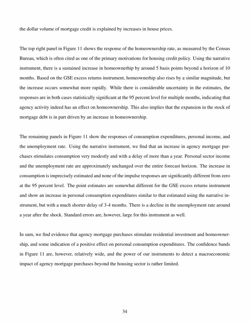
the dollar volume of mortgage credit is explained by increases in house prices.

The top right panel in Figure 11 shows the response of the homeownership rate, as measured by the Census

Bureau, which is often cited as one of the primary motivations for housing credit policy. Using the narrative

instrument, there is a sustained increase in homeownerhip by around 5 basis points beyond a horizon of 10

months. Based on the GSE excess returns instrument, homeownerhip also rises by a similar magnitude, but

the increase occurs somewhat more rapidly. While there is considerable uncertainty in the estimates, the

responses are in both cases statistically significant at the 95 percent level for multiple months, indicating that

agency activity indeed has an effect on homeownership. This also implies that the expansion in the stock of

mortgage debt is in part driven by an increase in homeownership.

The remaining panels in Figure 11 show the responses of consumption expenditures, personal income, and

the unemployment rate. Using the narrative instrument, we find that an increase in agency mortgage pur-

chases stimulates consumption very modestly and with a delay of more than a year. Personal sector income

and the unemployment rate are approximately unchanged over the entire forecast horizon. The increase in

consumption is imprecisely estimated and none of the impulse responses are significantly different from zero

at the 95 percent level. The point estimates are somewhat different for the GSE excess returns instrument

and show an increase in personal consumption expenditures similar to that estimated using the narrative in-

strument, but with a much shorter delay of 3-4 months. There is a decline in the unemployment rate around

a year after the shock. Standard errors are, however, large for this instrument as well.

In sum, we find evidence that agency mortgage purchases stimulate residential investment and homeowner-

ship, and some indication of a positive effect on personal consumption expenditures. The confidence bands

in Figure 11 are, however, relatively wide, and the power of our instruments to detect a macroeconomic

impact of agency mortgage purchases beyond the housing sector is rather limited.

34

7 Housing Credit Policy vs. Conventional Monetary Policy

In the previous section, we found that increases in agency mortgage purchases lead to an expansion in mort-

gage credit and to declines in short- and long-term interest rates. A natural question to ask is to what extent

these effects reflect conventional monetary policy actions, and how monetary and credit policies interact

more broadly. The left panel in Figure 12 reports the estimated response of the federal funds rate to an

agency purchase shock using the methods of the previous section. According to the narrative instrument,

there is a delayed and transitory decline in the funds rate by up to 30 basis points after 6 months. This

decrease is statistically significant after 4 to 12 months. The GSE excess returns instrument also yields a

temporary decline in the funds rate, but it is smaller in size and not statistically significant.

We obtain similar results for the post 1982 subsample, after excluding the non-borrowed reserves target-

ing period, or after omitting larger policy events from the narrative instrument (see online appendix A.4).

There is therefore evidence that agency mortgage purchases are accompanied by accommodative monetary

policy. A possible alternative interpretation is that both identification schemes erroneously pick up the in-

fluence of recessionary shocks causing downward adjustments in the Federal Reserve’s interest rate target.

However, if this were the case, we would not expect to find increases in strongly procyclical variables such as

mortgage originations or housing starts. To gain more insight into the nature of the funds rate response, we

make use of the decomposition by Romer and Romer (2004) of changes in the intended funds rate at FOMC

meetings into a systematic and a residual shock component.29 The systematic component is measured by the

explained variation in a regression of target changes on changes in Greenbook forecasts of inflation, output

growth, and unemployment. Monetary policy shocks are measured by the residuals in the regression, and

capture the remaining variation in target changes not explained by changes in the Greenbook forecasts.

The middle panel in Figure 12 depicts the estimated response of the cumulative Romer and Romer (2004)

shocks to an agency purchase shock using the regressions in (4) and (5). With a few months delay, the nar-

rative instrument yields a significant and persistent decline by up to 10 basis points. The funds rate decline

is therefore not explained by inflation and output considerations alone, and possibly reflects also an inde-

29We use the updates by Wieland and Yang (2016) to extend the sample of the original series.

35

pendent reaction to credit market conditions and/or credit policies. We note, however, that the GSE excess

returns instrument does not yield a similar significant decline in the Romer and Romer (2004) residual.

To investigate whether monetary policy affects housing credit policy, the right panel in Figure 12 reports

the response of the cumulated narrative measures of credit policy changes in Table 2, deflated by the core

PCE price index and as a percentage of trend originations, to a monetary shock. There is no evidence for

monetary policy shocks impacting the non-cyclical measure of agency purchase shocks, as our narratively

identified housing credit policy instrument is not itself predictable by the Romer and Romer (2004) residuals.

This provides assurance that our narrative instrument does not erroneously pick up the effects of monetary

policy shocks. Similarly, adding the current and lagged values of the Romer and Romer (2004) shocks as ad-

ditional control variables in (4) also has very little effect on the results, see online appendix A.4. The cyclical

housing policy measure (in red), on the other hand, does show a statistically significant decline following

an expansionary monetary policy shock, which illustrates the importance of accounting for the endogeneity

of credit policies. Consistent with an objective of stabilizing credit flows, we thus find that housing credit

policies on average act to offset the effects of monetary policy disturbances.

To further judge the extent to which agency purchase shocks operate through more conventional mone-

tary transmission channels, Figure 13 compares the impact of a traditional monetary policy shock (in red)

with the response to the agency purchase shock identified using the narrative instrument (in blue). The re-

sponse to a monetary shock is obtained by similar regressions as in equation (4), but replacing the agency

market share on the right hand side with the contemporaneous level of the 3-month T-bill rate, and using

the Romer and Romer (2004) shock measure as an instrument.30 In the figure, the impact of the interest

rate shock is scaled such that the maximum decline in the 3-month T-bill rate is the same as for the agency

purchase shock identified with the narrative instrument. For easier comparison, the responses to the mon-

etary policy shock in Figure 13 are shifted forward by 4 months such that the maximum interest declines

for each of the policy shocks coincide. As before, the bands are 95 percent Newey and West (1987) intervals.

30Conditional on including an informationally sufficient set of lagged variables as controls, valid identification under thisapproach requires only contemporaneous exogeneity of the Romer and Romer (2004) shocks. The predictability of the Romerand Romer (2004) shocks by agency purchase shock therefore does not necessarily invalidate the identification of the response tomonetary shocks.

36

Figure 13 reveals that conventional monetary policy shocks and credit policy shocks have qualitatively sim-

ilar effects on many of the variables shown. Although each of the policies involves purchases of different

types of assets with different sources of financing, both generate a decline in long-term interest rates, a rise

in originations and mortgage debt, and an increase in housing starts. Consistent with most of the existing

empirical literature, an expansionary monetary shock leads to increases in consumption and income and a

decline in the unemployment rate.31 The monetary shock responses provide a familiar reference point for

judging the quantitative impact of agency purchase shocks. After scaling the estimates to imply the same

decline in the short-term interest rate and accounting for the more immediate effects of a funds rate target

shock on short-term interest rates, many responses to each of the policy shocks are similar in terms of mag-

nitude and timing.

There are, however, also some notable differences between the responses in Figure 13. The first is that

agency purchases lead to a rise in originations that is roughly twice as large as that of the interest rate

shock. There is little indication that a conventional monetary policy shock causes a significant rise in real

house prices, while the decline in long-term interest rates is slightly more pronounced and persistent after an

agency purchase shock. Both the rise in housing starts and mortgage debt, on the other hand, are very simi-

lar for both policy shocks. Taken together, the results indicate that agency purchases have a larger effect on

mortgage repayments than conventional interest rate policy. In appendix A.3, we compare the responses of

refinance and purchase originations. Whereas purchase originations respond very similarly to both shocks,

refinancing originations react more strongly to the agency purchase shock, and account for the entire differ-

ence in the effect on total originations.

Another notable difference between credit policy and traditional interest rate shocks is the effect on the

homeownership rate (right panel, third row in Figure 13). Unlike the response to an agency purchase shock,

there is no indication that a conventional interest rate shock has any positive effect on homeownership. In

most months, the estimated effect on homeownership instead is negative, though small and generally not sta-

31The response to both shocks also feature a similar ‘price puzzle’, i.e. a decline in the price level as measured by the PCE priceindex. Results are available on request.

37

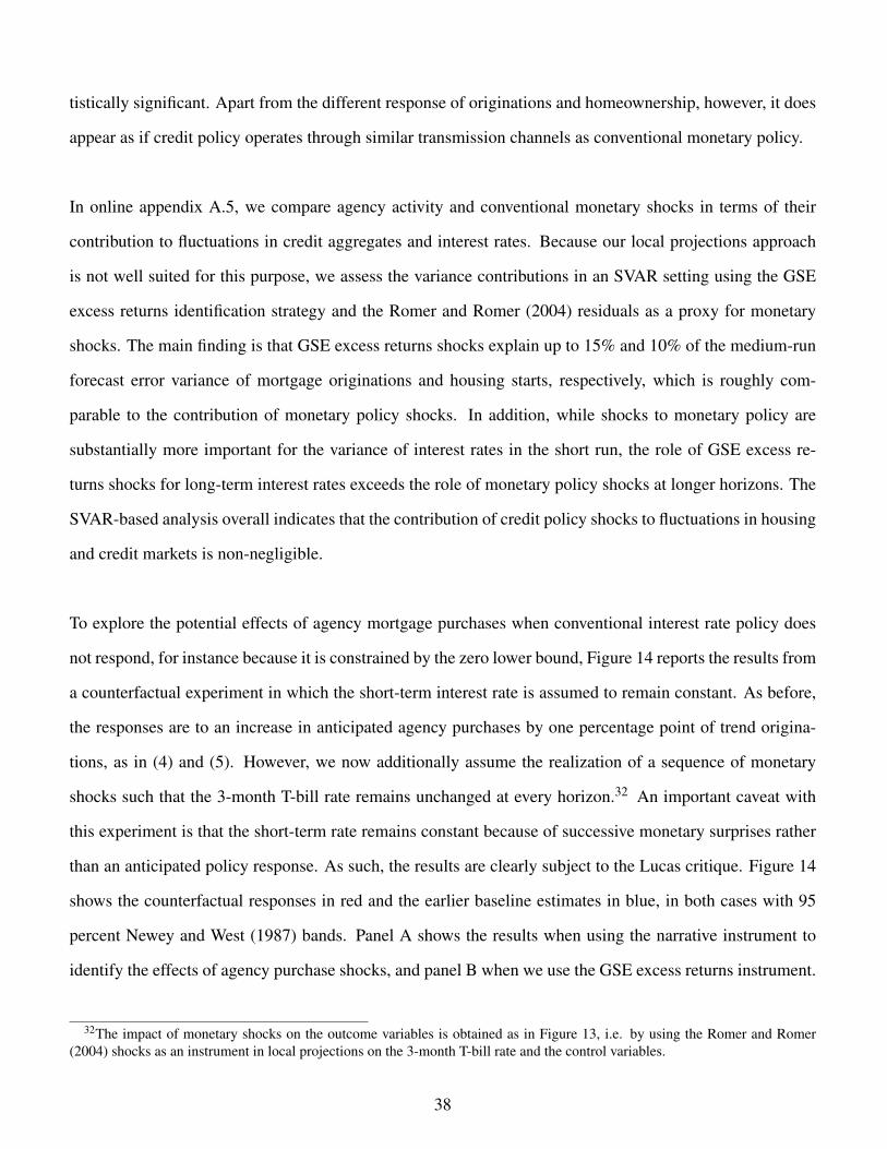
tistically significant. Apart from the different response of originations and homeownership, however, it does

appear as if credit policy operates through similar transmission channels as conventional monetary policy.

In online appendix A.5, we compare agency activity and conventional monetary shocks in terms of their

contribution to fluctuations in credit aggregates and interest rates. Because our local projections approach

is not well suited for this purpose, we assess the variance contributions in an SVAR setting using the GSE

excess returns identification strategy and the Romer and Romer (2004) residuals as a proxy for monetary

shocks. The main finding is that GSE excess returns shocks explain up to 15% and 10% of the medium-run

forecast error variance of mortgage originations and housing starts, respectively, which is roughly com-

parable to the contribution of monetary policy shocks. In addition, while shocks to monetary policy are

substantially more important for the variance of interest rates in the short run, the role of GSE excess re-

turns shocks for long-term interest rates exceeds the role of monetary policy shocks at longer horizons. The

SVAR-based analysis overall indicates that the contribution of credit policy shocks to fluctuations in housing

and credit markets is non-negligible.

To explore the potential effects of agency mortgage purchases when conventional interest rate policy does

not respond, for instance because it is constrained by the zero lower bound, Figure 14 reports the results from

a counterfactual experiment in which the short-term interest rate is assumed to remain constant. As before,

the responses are to an increase in anticipated agency purchases by one percentage point of trend origina-

tions, as in (4) and (5). However, we now additionally assume the realization of a sequence of monetary

shocks such that the 3-month T-bill rate remains unchanged at every horizon.32 An important caveat with

this experiment is that the short-term rate remains constant because of successive monetary surprises rather

than an anticipated policy response. As such, the results are clearly subject to the Lucas critique. Figure 14

shows the counterfactual responses in red and the earlier baseline estimates in blue, in both cases with 95

percent Newey and West (1987) bands. Panel A shows the results when using the narrative instrument to

identify the effects of agency purchase shocks, and panel B when we use the GSE excess returns instrument.

32The impact of monetary shocks on the outcome variables is obtained as in Figure 13, i.e. by using the Romer and Romer(2004) shocks as an instrument in local projections on the 3-month T-bill rate and the control variables.

38

The results from the counterfactual experiment in Figure 14 indicate that conventional monetary policy plays

an important role in explaining the effects of agency purchase shocks. Under both identification schemes,

the rise in originations is only about half as large when short-term interest rates remain constant, and there is

no longer any sign of an increase in the stock of mortgage debt. The drop in long-term interest rates is much

reduced with the narrative instrument, but remains more clearly present with the excess returns instrument.

The positive effect on housing starts is smaller using the GSE excess returns instrument, and disappears

entirely with the narrative instrument. The combination of expansionary monetary and credit policy there-

fore seems particularly important for stimulating residential investment. Even with constant interest rates,

however, purchases of mortgage assets continue to have statistically significant effects on mortgage lending,

regardless of the instrument. In addition, the path of short-term interest rates appears largely irrelevant for

the increase in the homeownership rate following a shock to agency purchases.

8 Concluding Remarks

The postwar period witnessed a remarkable expansion in residential mortgage debt. During the same period,

an increasing share has come to reside on what is ultimately the balance sheet of the federal government.

In this paper, we provide evidence that government mortgage purchases influence the volume and cost of

mortgage lending. In order to tackle reverse causality, we make use of a number of policy changes that have

impacted the ability of government agencies to acquire mortgage debt. Using policy interventions that we

classify as non-cyclically motivated to construct an instrumental variable for (news about) agency mortgage

purchases, we find that an increase in these purchases stimulates mortgage originations and debt, and tem-

porarily lowers mortgage rates. Consistent with the evidence in Di Maggio et al. (2016) regarding the effects

of the QE interventions, we find that agency purchases have particularly large effects on refinancing activity.

We also find a positive impact on housing starts and homeownership, and some indications of positive effects

on house prices and consumption expenditures. An alternative identification strategy based on instrumenting

with orthogonalized innovations in GSE excess returns yields very similar results overall.

One important aspect of our findings is the apparent similarity and interaction between housing credit poli-

cies and conventional interest rate policy. We find that greater agency mortgage purchases lead to broad

39

declines in short and long-term interest rates. Our measure of non-cyclically motivated credit policy changes

predicts the Romer and Romer (2004) monetary policy shock measure, and expansionary credit policy ap-

pears to be accommodated by monetary policy. In contrast, we find that credit policy adjusts in order to

offset the effects of monetary disturbances. It may therefore be necessary to account for credit policy to un-

derstand the effects of monetary policy. Agency purchase shocks have relatively larger effects on mortgage

originations and refinancing activity than interest rate shocks, and influence homeownership regardless of

the path of short-term interest rates. The quantitative effects of credit and monetary policy shocks on many

other variables, including residential investment, are otherwise remarkably similar.

There are several interesting avenues for future research: Unlike theoretical or multivariate statistical models,

our local projections/IV-approach does not allow an assessment of the historical contribution of structural

shocks without further assumptions. In online appendix A.5, we apply our GSE excess returns identification

strategy in an SVAR setting, and we find that the contribution to the short-run variability of mortgage credit

and housing starts is substantial and similar to that of monetary policy shocks. Future work can verify in

more detail whether credit policy shocks are important causal factors in past housing or credit cycles, in

particular during the most recent housing boom and bust.33 Our results can be used to help evaluate the

credit policy interventions in the recent financial crisis, the possible impact of unwinding the Fed’s current

mortgage holdings, or the various proposals for GSE reform. We have made no attempt at understanding

more precisely the nature or implications of the credit frictions and transmission channels through which

housing credit policies operate. Future work may apply similar cross-sectional identification strategies as Di

Maggio et al. (2016), Darmouni and Rodnyansky (2016), or Chakraborty, Goldstein, and MacKinlay (2016)

to other housing credit policy events documented in our narrative analysis. Finally, it is possible to apply a

similar analysis to government mortgage guarantees and securitization.

33The expansion of the GSE’s market share from the early 1990s to mid-2004 was dramatic, but came to a grinding halt when,following revelations of accounting fraud, regulators imposed capital surcharges on Fannie and Freddie in the fall of 2004 andeventually portfolio caps in mid-2006.

40

References

Arcelus, Francisco and Allan H. Meltzer, “The Markets for Housing and Housing Services,” Journal ofMoney, Credit and Banking, 5 (1973), 78–99.

Bassett, William F., Mary Beth Chosak, John C. Driscoll, and Egon Zakrajsek, “Changes in Bank LendingStandards and the Macroeconomy,” Journal of Monetary Economics, 62 (2014), 23–40.

Bordo, Michael D. and Joseph G. Haubrich, “Credit Crises, Money and Contractions: An Historical View,”Journal of Monetary Economics, 57 (2010), 1–18.

Boudoukh, Jacob, Matthew Richardson, Richard Stanton, and Robert F. Whitelaw, “Pricing Mortgage-Backed Securities in a Multifactor Interest Rate Environment: A Multivariate Density Estimation Ap-proach,” The Review of Financial Studies, 10 (1997), 405–446.

Chakraborty, Indraneel, Itay Goldstein, and Andrew MacKinlay, “Monetary Stimulus and Bank Lending,”University of Miami manuscript, 2016.

Congressional Research Service, “A Chronology of Housing Legislation and Selected Executive Actions,1892-2003,” Washington, D.C: U.S. Government Printing Office, 2004.

Curdia, Vasco and Michael Woodford, “The Central-Bank Balance Sheet as an Instrument of MonetaryPolicy,” Journal of Monetary Economics, 58 (2011), 54–79.

Darmouni, Olivier and Alexander Rodnyansky, “The Effects of Quantitative Easing on Bank Lending Be-havior,” forthcoming, Review of Financial Studies, 2017.

Davis, Morris A. and Jonathan Heathcote, “The Price and Quantity of Residential Land in the United States,”Journal of Monetary Economics, 54 (2007), 2595–2620.

Di Maggio, Marco and Amir Kermani, “Credit-Induced Boom and Bust,” forthcoming, Review of FinancialStudies, 2016.

Di Maggio, Marco, Amir Kermani, and Christopher Palmer, “How Quantitative Easing Works: Evidence onthe Refinancing Channel,” Columbia Business School Research Paper No. 16-1, 2016.

Eckstein, Otto and Allen Sinai, “The Mechanisms of the Business Cycle in the Postwar Era”, in The Ameri-can Business Cycle: Continuity and Change, Robert J. Gordon, ed. (Chicago, IL: NBER and The Univer-sity of Chicago Press, 1986).

Fieldhouse, Andrew and Karel Mertens, “A Narrative Analysis of Mortgage Asset Purchases by FederalAgencies,” NBER Working Paper No. 23165, 2017.

Fisher, Jonas D.M. and Ryan Peters, “Using Stock Returns to Identify Government Spending Shocks,” TheEconomic Journal, 120 (2010), 414–436.

Gagnon, Joseph, Matthew Raskin, Julie Remache, and Brian Sack, “The Financial Market Effects of theFederal Reserve’s Large-Scale Asset Purchases,” International Journal of Central Banking, 7 (2011),3–43.

Gertler, Mark and Nobuhiro Kiyotaki, “Financial Intermediation and Credit Policy in Business Cycle Anal-ysis,” in Handbook of Monetary Economics, Volume 3A, Benjamin M. Friedman and Michael Woodford,eds. (San Diego, CA: North-Holland, 2010).

Gilchrist, Simon and Egon Zakrajsek, “Credit Spreads and Business Cycle Fluctuations,” American Eco-nomic Review, 102 (2012), 1692–1720.

Greenspan, Alan, “Government-Sponsored Enterprises,” Remarks by Chairman Alan Greenspan to the Con-ference on Housing, Mortgage Finance, and the Macroeconomy, Federal Reserve Bank of Atlanta, At-lanta, Georgia, May 19, 2005.

Gonzalez-Rivera, Gloria, “Linkages Between Secondary and Primary Markets for Mortgages,” The Journalof Fixed Income, 11 (2001), 29–36.

41

Haltum, Renee and Robert Sharp, “The First Time the Fed Bought GSE Debt,” Federal Reserve Bank ofRichmond Economic Brief 14-04, 2014.

Hancock, Diana and Wayne Passmore, “Did the Federal Reserve’s MBS Purchase Program Lower MortgageRates?,” Journal of Monetary Economics, 58 (2011), 498–514.

Hancock, Diana and Wayne Passmore, “How Does the Federal Reserve’s Large-Scale Asset Purchases(LSAPs) Influence Mortgage-Backed Securities (MBS) Yields and U.S. Mortgage Rates?,” Real EstateEconomics, 43 (2015), 855–890.

Hanson, Samuel G., “Mortgage Convexity,” Journal of Financial Economics, 113 (2014), 270–299.Hendershott, Patric H. and Kevin E. Villani, “The Federally Sponsored Credit Agencies: Their Behavior

and Impact,” in Capital Markets and the Housing Sector: Perspectives on Financial Reform, Robert M.Buckley, John A. Tucillo, and Kevin Villani, eds. (Cambridge, MA: Ballinger Publishing Co., 1977).

Hendershott, Patric H. and Kevin E. Villani, “Residential Mortgage Markets and the Cost of MortgageFunds,” Journal of the American Real Estate and Urban Economics Association, 8 (1980), 50–76.

Hendershott, Patric H. and James D. Shilling, “The Impact of the Agencies on Conventional Fixed-RateMortgage Yields,” Journal of Real Estate Finance and Economics, 2 (1989), 101-115.

Jaffee, Dwight M. and Kenneth T. Rosen, “Estimates of the Effectiveness of Stabilization Policies for theMortgage and Housing Markets,” Journal of Finance, 33 (1978), 933-946.

Jorda, Oscar, “Estimation and Inference of Impulse Responses by Local Projections,” American EconomicReview, 95 (2005), 161–182.

Justiniano, Alejandro, Giorgio E. Primiceri, and Andrea Tambalotti, “Credit Supply and the Housing Boom,”NBER Working Paper No. 20874, 2015.

Kaufman, Herbert M., “FNMA and the Housing Cycle: Its Recent Contribution and Its Future Role ina Deregulated Environment,” in The Federal National Mortgage Association in a Changing EconomicEnvironment, Supplement to a Report by the Comptroller General of the United States. (Washington,D.C.: U.S. Government Accountability Office, 1985).

Krishnamurthy, Arvind and Annette Vissing-Jørgensen, “The Effects of Quantitative Easing on InterestRates: Channels and Implications for Policy,” Brookings Papers on Economic Activity, 3 (2011), 215–265.

Leamer, Edward E., “Housing IS the Business Cycle,” NBER Working Paper No. 13428, 2007.Lehnert, Andreas, Wayne Passmore, and Shane M. Sherlund, “GSEs, Mortgage Rates, and Secondary Mar-

ket Activities,” Journal of Real Estate Finance and Economics, 36 (2008), 343-363.Malkhozov, Aytek, Philippe Mueller, Andrea Vedolin, and Gyuri Venter, “Mortgage Risk and the Yield

Curve,” The Review of Financial Studies 29 (2016), 1220–1253.Meltzer, Allan H., “Credit Availability and Economic Decisions: Some Evidence from the Mortgage and

Housing Markets,” Journal of Finance, 29 (1974), 763–777.Mertens, Karel and Morten O. Ravn, “Empirical Evidence on the Aggregate Effects of Anticipated and

Unanticipated US Tax Policy Shocks,” American Economic Journal: Economic Policy, 4 (2012), 145–181.

Mian, Atif and Amir Sufi, “The Consequences of Mortgage Credit Expansion: Evidence from the U.S.Mortgage Default Crisis,” Quarterly Journal of Economics, 124 (2009), 1449–1496.

Mian, Atif, Amir Sufi, and Emil Verner, “How Do Credit Supply Shocks Affect the Real Economy? Evidencefrom the United States in the 1980s,” Princeton University manuscript, 2017.

Naranjo, Andy and Alden Toevs, “The Effects of Purchases of Mortgages and Securitization by GovernmentSponsored Enterprises on Mortgage Yield Spreads and Volatility,” Journal of Real Estate Finance andEconomics, 25 (2002), 173–195.

Newey, Whitney K. and Kenneth D. West, “A Simple, Positive Semi-Definite, Heteroskedasticity and Auto-

42

correlation Consistent Covariance Matrix,” Econometrica, 55 (1987), 703–708.Owens, Raymond E. and Stacey L. Schreft, “Identifying Credit Crunches,” Federal Reserve Bank of Rich-

mond Working Paper 93-02, 1993.Patrabansh, Saty, William M. Doerner, and Samuel Asin, “The Effect of Monetary Policy on Mortgage

Rates,” FHFA Working Paper 14-2, 2014.Passmore, S. Wayne, “The GSE Implicit Subsidy and the Value of Government Ambiguity,” FEDS Working

Paper No. 2005-05, 2005.Peek, Joe, Eric S. Rosengren, and Geoffrey M.B. Tootell, “Identifying the Macroeconomic Effects of Loan

Supply Shocks,” Journal of Money, Credit and Banking, 35 (2003), 931–946.Perli, Roberto, and Brian P. Sack, “Does Mortgage Hedging Amplify Movements in Long-Term Interest

Rates?,” The Journal of Fixed Income, 13 (2003), 7–17.Ramey, Valerie A., “Identifying Government Spending Shocks: It’s All in the Timing,” Quarterly Journal of

Economics, 126 (2011), 1–50.Ramey, Valerie A., “Macroeconomic Shocks and Their Propagation,” in Handbook of Macroeconomics,

Volume 2A, John B. Taylor and Herald Uhlig, eds. (San Diego, CA: North-Holland, 2016).Ramey, Valerie A. and Sarah Zubairy, “Government Spending Multipliers in Good Times and in Bad: Evi-

dence from U.S. Historical Data,” University of California, San Diego manuscript, 2016.Romer, Christina D. and David H. Romer, “Does Monetary Policy Matter? A New Test in the Spirit of

Friedman and Schwartz,” in NBER Macroeconomics Annual 1989, Volume 4, Olivier Jean Blanchard andStanley Fischer, eds. (Cambridge, MA: The MIT Press, 1989).

Romer, Christina D. and David H. Romer, “A New Measure of Monetary Shocks: Derivation and Implica-tions,” American Economic Review, 94 (2004), 1055–1084.

Romer, Christina D. and David H. Romer, “The Macroeconomic Effects of Tax Changes: Estimates Basedon a New Measure of Fiscal Shocks,” American Economic Review, 100 (2010), 763–801.

Shiller, Robert J., Irrational Exuberance, 3rd ed. (Princeton, NJ: Princeton University Press, 2015).Shumway, R.H. and D.S. Stoffer, “An Approach to Time Series Smoothing and Forecasting Using the EM

Algorithm,” Journal of Time Series Analysis, 3 (1982), 253–264.Smith, Lawrence B., Kenneth T. Rosen, and George Fallis, “Recent Developments in Economic Models of

Housing Markets,” Journal of Economic Literature, 26 (1988), 29–64.Stroebel, Johannes and John B. Taylor, “Estimated Impact of the Federal Reserve’s Mortgage-Backed Secu-

rities Purchase Program,” International Journal of Central Banking, 8 (2012), 1–42.Wieland, Johannes F. and Mu-Yeung Yang, “Financial Dampening,” University of California, San Diego

manuscript, 2016.

43

Residential Mortgage Debt

1900 1910 1920 1930 1940 1950 1960 1970 1980 1990 2000 2010

10

20

30

40

50

60

70

80

90

Percent

As Ratio of GDP

As Ratio of Residential Wealth

Residential Mortgage Originations

1955 1960 1965 1970 1975 1980 1985 1990 1995 2000 2005 2010

10

20

30

40

50

60

Percent

As Ratio of GDP

As Ratio of Residential Mortgage Debt

Agency Mortgage Holdings

1930 1940 1950 1960 1970 1980 1990 2000 20100

5

10

15

20

25

Percent of Total Mortgage Debt

TotalTotal excl. Federal ReserveFNMA,FHLMC & GNMA

Agency Purchases and Pool Issuance

1955 1960 1965 1970 1975 1980 1985 1990 1995 2000 2005 2010

0

20

40

60

80

100

120

140

Percent of Total Originations

Total Net Portfolio PurchasesTotal Net Portfolio Purchases excl. Federal ReserveAgency Pool Issues

Figure 1 Mortgage Debt, Annualized Originations, and Agency Market Shares

Notes: Residential mortgage debt and originations include home as well as multifamily mortgages. Agency holdings includeholdings of both whole loans and pools. Agency purchases are net purchases for portfolio investment, whereas pool issuesapproximate purchases backing new issuance of mortgage pools (mortgage-backed securities). The grey bars are NBER-datedrecessions. Sources: see data appendix.

44

-8 -6 -4 -2 0 2 4 6 8 10 12Quarters from Peak

-20

-10

0

10

20

30

40

Log Difference with Peak

Recessions

Agency Held

Agency Held excl. Great Recession

Privately Held

Privately Held excl. Great Recession

-8 -6 -4 -2 0 2 4 6 8 10 12Quarters from Peak

-20

-10

0

10

20

30

40

Log Difference with Peak

Credit Crunches

Agency Held

Agency Held excl. 2007 Financial Crisis

Privately Held

Privately Held excl. 2007 Financial Crisis

Figure 2 Real Mortgage Debt by Holder in Recessions and Credit Crunches

Notes: Mortgage debt is deflated by the core PCE price index. Left panel: average of 9 NBER recessions starting 1957Q2,1960Q1, 1969Q4, 1973Q4, 1980Q1, 1981Q3, 1990Q3, 2001Q1, 2007Q4. Right panel: average of credit crunches beginning onequarter after the following dates: 1955Q3, 1959Q1, 1965Q4, 1968Q4, 1972Q4, 1978Q1, 1980Q4, 1990Q1, 1998Q2, 2007Q2.See data appendix for sources.

1970 1975 1980 1985 1990 1995 2000 2005 2010 2015

-4

-2

0

2

4

6

Percent of Trend Originations

Not Cyclically Motivated

1970 1975 1980 1985 1990 1995 2000 2005 2010 2015

0

10

20

30

40

50

Percent of Trend Originations

Cyclically Motivated

Figure 3 Measures of Policy Events Affecting Agency Mortgage Holdings: Jan 1967 to Dec 2014

Notes: The figure shows projected changes in the consolidated agency mortgage portfolio as a percentage of average annualizedmortgage originations over the prior twelve months. The left panel shows changes classified as unrelated to the business orfinancial cycle. The right panel shows changes classified as primarily motivated by cyclical considerations. For sources andclassification see Fieldhouse and Mertens (2017). Shaded areas are credit crunch periods, see data appendix for chronology.

45

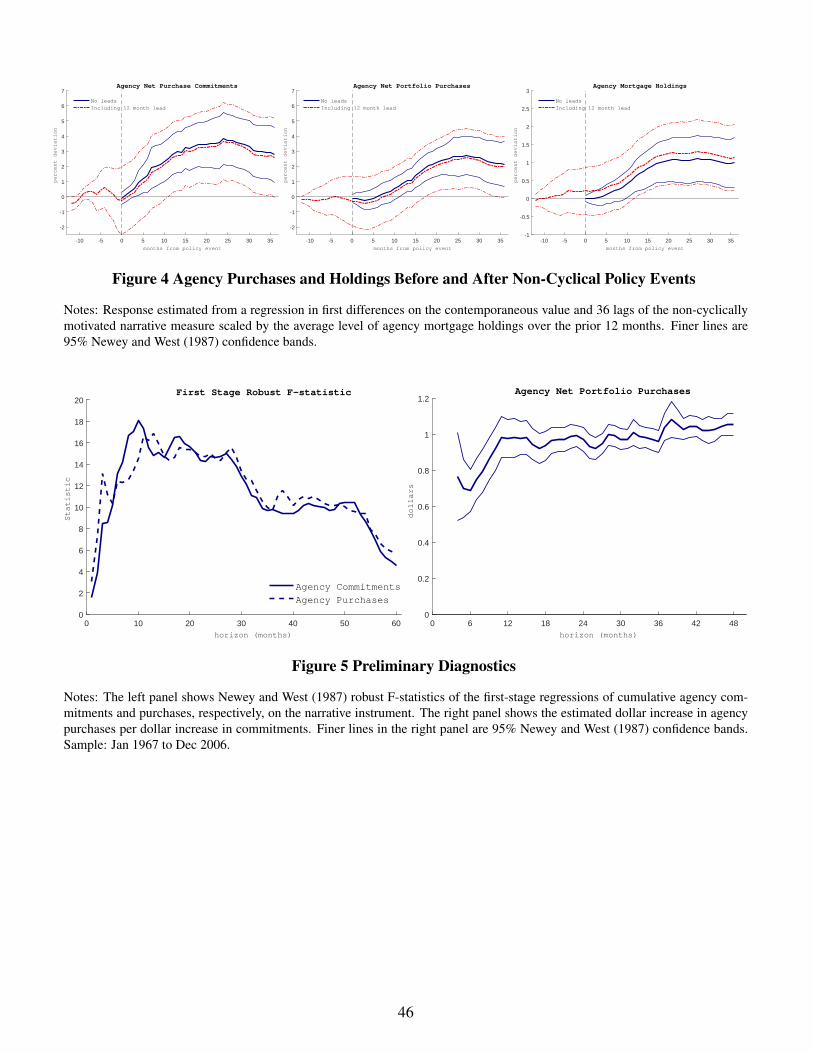
-10 -5 0 5 10 15 20 25 30 35months from policy event

-2

-1

0

1

2

3

4

5

6

7

percent deviation

Agency Net Purchase Commitments

No leads

Including 12 month lead

-10 -5 0 5 10 15 20 25 30 35months from policy event

-2

-1

0

1

2

3

4

5

6

7

percent deviation

Agency Net Portfolio Purchases

No leads

Including 12 month lead

-10 -5 0 5 10 15 20 25 30 35months from policy event

-1

-0.5

0

0.5

1

1.5

2

2.5

3

percent deviation

Agency Mortgage Holdings

No leads

Including 12 month lead

Figure 4 Agency Purchases and Holdings Before and After Non-Cyclical Policy Events

Notes: Response estimated from a regression in first differences on the contemporaneous value and 36 lags of the non-cyclicallymotivated narrative measure scaled by the average level of agency mortgage holdings over the prior 12 months. Finer lines are95% Newey and West (1987) confidence bands.

0 10 20 30 40 50 60horizon (months)

0

2

4

6

8

10

12

14

16

18

20

Statistic

First Stage Robust F-statistic

Agency Commitments

Agency Purchases

0 6 12 18 24 30 36 42 48horizon (months)

0

0.2

0.4

0.6

0.8

1

1.2dollars

Agency Net Portfolio Purchases

Figure 5 Preliminary Diagnostics

Notes: The left panel shows Newey and West (1987) robust F-statistics of the first-stage regressions of cumulative agency com-mitments and purchases, respectively, on the narrative instrument. The right panel shows the estimated dollar increase in agencypurchases per dollar increase in commitments. Finer lines in the right panel are 95% Newey and West (1987) confidence bands.Sample: Jan 1967 to Dec 2006.

46

0 6 12 18 24 30 36 42 48horizon (months)

0

0.2

0.4

0.6

0.8

1

1.2

dollars

Agency Mortgage Holdings

Agency Commitments

Agency Purchases

0 6 12 18 24 30 36 42 48horizon (months)

-2.5

-2

-1.5

-1

-0.5

0

0.5

1

1.5

dollars

Private Mortgage Holdings

Agency Commitments

Agency Purchases

0 6 12 18 24 30 36 42 48horizon (months)

-1

0

1

2

3

4

5

dollars

Mortgage Originations: Total

Agency Commitments

Agency Purchases

0 6 12 18 24 30 36 42 48horizon (months)

-1

-0.5

0

0.5

1

1.5

dollars

Residential Mortgage Debt

Agency Commitments

Agency Purchases

0 6 12 18 24 30 36 42 48horizon (months)

-0.5

0

0.5

1

1.5

2

2.5

3

3.5

4

dollars

Mortgage Originations: Refinancing

Agency Commitments

Agency Purchases

0 6 12 18 24 30 36 42 48horizon (months)

-1

-0.5

0

0.5

1

1.5

dollars

Mortgage Originations: Purchase

Agency Commitments

Agency Purchases

Figure 6 Estimated Balance Sheet Adjustments and Mortgage Credit Multipliers Associated withAgency Mortgage Purchases

Notes: The figure shows dollar changes per dollar increase in agency net portfolio purchases or commitments to purchase cumu-lated over the reported horizon in months. Estimates are from local projections-IV regressions, see equation (2). Finer lines are95% Newey and West (1987) confidence bands. Sample: Jan 1967 to Dec 2006. In the bottom row panels, the sample excludesMay 1985 to Dec 1986 because of missing data on refinance shares, see data appendix.

47

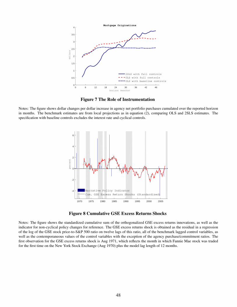
0 6 12 18 24 30 36 42 48horizon (months)

0

0.5

1

1.5

2

2.5

3

3.5

4

dollars

Mortgage Originations

2SLS with full controls

OLS with full controls

OLS with baseline controls

Figure 7 The Role of Instrumentation

Notes: The figure shows dollar changes per dollar increase in agency net portfolio purchases cumulated over the reported horizonin months. The benchmark estimates are from local projections as in equation (2), comparing OLS and 2SLS estimates. Thespecification with baseline controls excludes the interest rate and cyclical controls.

1970 1975 1980 1985 1990 1995 2000 2005

-4

-2

0

2

4

6

percent

Narrative Policy Indicator

Cum. GSE Excess Return Shocks (Standardized)

Figure 8 Cumulative GSE Excess Returns Shocks

Notes: The figure shows the standardized cumulative sum of the orthogonalized GSE excess returns innovations, as well as theindicator for non-cyclical policy changes for reference. The GSE excess returns shock is obtained as the residual in a regressionof the log of the GSE stock price-to-S&P 500 ratio on twelve lags of this ratio, all of the benchmark lagged control variables, aswell as the contemporaneous values of the control variables with the exception of the agency purchase/commitment ratios. Thefirst observation for the GSE excess returns shock is Aug 1971, which reflects the month in which Fannie Mae stock was tradedfor the first time on the New York Stock Exchange (Aug 1970) plus the model lag length of 12 months.

48

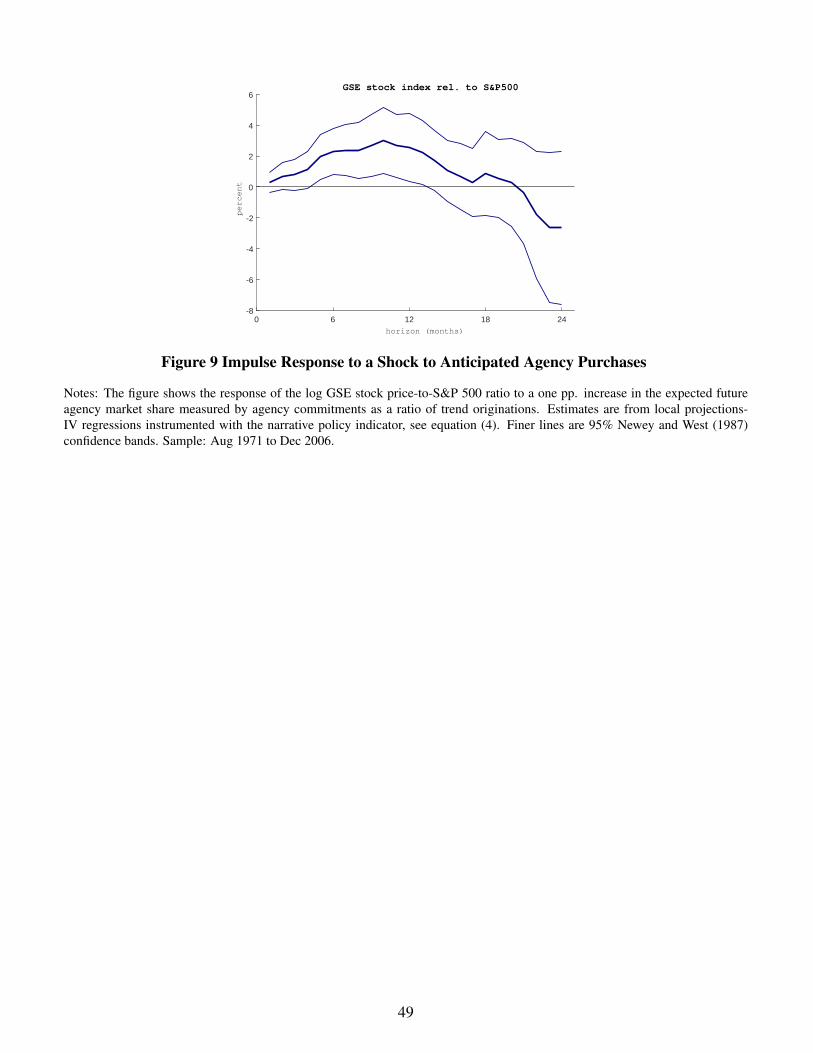
0 6 12 18 24horizon (months)

-8

-6

-4

-2

0

2

4

6

percent

GSE stock index rel. to S&P500

Figure 9 Impulse Response to a Shock to Anticipated Agency Purchases

Notes: The figure shows the response of the log GSE stock price-to-S&P 500 ratio to a one pp. increase in the expected futureagency market share measured by agency commitments as a ratio of trend originations. Estimates are from local projections-IV regressions instrumented with the narrative policy indicator, see equation (4). Finer lines are 95% Newey and West (1987)confidence bands. Sample: Aug 1971 to Dec 2006.

49

Figure 10 Impulse Responses to a Shock to Anticipated Agency Purchases

Notes: The figure shows responses to a one pp. increase in the expected future agency market share measured by agency commit-ments as a ratio of trend originations. Estimates are from local projections-IV regressions instrumented with the narrative policyindicator, see equation (4), or orthogonalized GSE excess stock returns innovations, see equation (5). Finer lines and shaded areasare 95% Newey and West (1987) confidence bands. Sample: Jan 1967 to Dec 2006.

50

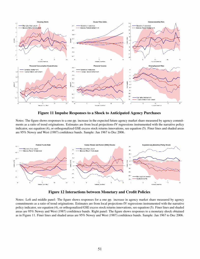
Figure 11 Impulse Responses to a Shock to Anticipated Agency Purchases

Notes: The figure shows responses to a one pp. increase in the expected future agency market share measured by agency commit-ments as a ratio of trend originations. Estimates are from local projections-IV regressions instrumented with the narrative policyindicator, see equation (4), or orthogonalized GSE excess stock returns innovations, see equation (5). Finer lines and shaded areasare 95% Newey and West (1987) confidence bands. Sample: Jan 1967 to Dec 2006.

Figure 12 Interactions between Monetary and Credit Policies

Notes: Left and middle panel: The figure shows responses for a one pp. increase in agency market share measured by agencycommitments as a ratio of trend originations. Estimates are from local projections-IV regressions instrumented with the narrativepolicy indicator, see equation (4), or orthogonalized GSE excess stock returns innovations, see equation (5). Finer lines and shadedareas are 95% Newey and West (1987) confidence bands. Right panel: The figure shows responses to a monetary shock obtainedas in Figure 11. Finer lines and shaded areas are 95% Newey and West (1987) confidence bands. Sample: Jan 1967 to Dec 2006.

51

Figure 13 Responses to A Shock to Anticipated Agency Purchases Versus a Monetary Policy Shock

Notes: The figure shows responses to a one pp. increase in the expected future agency market share as well as the response to amonetary policy shock. Estimates are from local projections-IV regressions instrumenting agency commitments with the narrativepolicy indicator, see equation (4), and instrumenting the 3 month T-bill rate with the Romer and Romer (2004) monetary policyshock measure. Finer lines and shaded areas are 95% Newey and West (1987) confidence bands. Sample: Jan 1967 to Dec 2006.

52

A. Narrative Instrument

B. GSE Excess Returns Instrument

Figure 14 Shock to Anticipated Agency Purchases: Counterfactual with Constant Short-Term Rate

Notes: The figure shows responses to a one pp. increase in the expected future agency market share and a sequence of monetaryshocks such that the 3-month T-bill rate remains constant. Estimates are from local projections-IV regressions instrumentingagency commitments with the narrative policy indicator. Finer lines and shaded areas are 95% Newey and West (1987) confidencebands. Sample: Jan 1967 to Dec 2006.

53

Table 1: Sources for Narrative Analysis

Government PublicationsBoard of Governors Annual Report, Press releases, Federal Reserve BulletinCongressional Budget Office The Housing Finance System and Federal Policy: Recent Changes and Options for

the Future (1983), Controlling Risks of Government-Sponsored Enterprises (1991)Congressional Quarterly Congressional Quarterly AlmanacCongressional Research Service A Chronology of Housing Legislation and Selected Executive Actions, 1892-2003

(2004), The Conforming Loan Limit (2008)Council of Economic Advisors Economic Report of the PresidentDepartment of Housing and UrbanDevelopment

HUD news releases, The Secondary Market in Residential Mortgages (1982), 1986Report to Congress on the Federal National Mortgage Association (1987), TheNational Homeownership Strategy: Partners in the American Dream (1995),Privatization of Fannie Mae and Freddie Mac: Desirability and Feasibility (1996),Profiles of GSE Mortgage Purchases in 2001-2004 (2008)

Department of the Treasury Press releases and statements, Report of the Secretary of the Treasury onGovernment-Sponsored Enterprises (1990), Government Sponsorship of the FNMAand the FHLMC (1996)

Federal Home Loan MortgageCorporation

Press releases and statements, Annual Report, Form 10-K

Federal Housing Finance Administration Press releases and statements, Mortgage Market NotesFederal National Mortgage Association Press releases and statements, Annual Report, Form 10-K, Monthly Volume

Summary, Information Statement, MBSenger, Offering Circular, Background andHistory of the Federal National Mortgage Association (1969, 1973)

Financial Crisis Inquiry Commission Final Report of the Financial Crisis Inquiry Commission (2011)Government Accountability Office The Federal National Mortgage Association in a Changing Environment (1985),

GSEs: A Framework for Limiting the Government’s Exposure to Risk (1991),Housing Enterprises: Potential Impacts of Severing Government Sponsorship (1996),HUD’s Mission Oversight Needs to be Strengthened (1998)

US Congress Hearing transcripts and reports: Committees on Appropriations, Committees onBanking and Currency, Committee on Banking, Finance and Urban Affairs, andCommittee on Banking, Housing and Urban Affairs

Office of Federal Housing EnterpriseOversight

Press releases and statements, Annual Report, Mortgage Market Notes, MortgageMarkets and the Enterprises, Evaluating the Capital Adequacy of Freddie Mac andFannie Mae (1998), Special Examination Reports (2003, 2004, 2006)

Office of the Federal Register Federal RegisterOffice of Management and Budget Budget of the United States GovernmentThe President’s Commission on Housing The Report of The President’s Commission on Housing (1982)

Press and Online Sources ABA Banking Journal, American Banker, The American Presidency Project, TheBond Buyer, Dow Jones Capital Market Reports, Dow Jones News Service, DowJones Newswires, Financial Times, MarketWatch, National Mortgage News, The NewYork Times, Reuters News, The Wall Street Journal, The Washington Post

Overview Books and ArticlesBartke Fannie Mae and the Secondary Mortgage Market (1971), Home Financing at a

Crossroads: A Study of the Federal Home Loan Mortgage Corporation (1973)Elliot, Feldberg, and Lehnert The History of Cyclical Macroprudential Policy in the US (2013)Greenspan The Age of Turbulence: Adventures in a New World (2007)Haar Federal Credit and Private Housing: The Mass Financing Dilemma (1960)Hagerty The Fateful History of Fannie Mae: New Deal Birth to Mortgage Crisis Fall (2012)Hoffman and Cassell Mission Expansion in the Federal Home Loan Bank System (2010)Hunter The FNMA: Its Response to Critical Financing Requirements of Housing (1971)McLean Shaky Ground: The Strange Saga of the US Mortgage Giants (2015)

Notes: For detailed bibliographical references, see Fieldhouse and Mertens (2017).

54

Table 2: Narrative Measures of Policy Changes

Policy Description Agency Impact News Effective ClassificationHUDA 1968: Special Assistance GNMA +$0.25 billion Aug. 1968 July 1969 Non-CyclicalHUDA 1968: Increased Debt-to-Capital Ratio FNMA +$1.39 billion Oct. 1968 Oct. 1968 Non-CyclicalIncreased Debt-to-Capital Ratio FNMA +$1.13 billion Dec. 1969 Dec. 1969 CyclicalHUDA 1969: Special Assistance GNMA +$0.75 billion Dec. 1969 Dec. 1969 CyclicalTreasury-Guaranteed Capitalization FNMA +$2.6 billion Apr. 1970 Apr. 1970 CyclicalEHFA 1970: Special Assistance GNMA +$0.38 billion July 1970 July 1970 CyclicalConforming Mortgage Program Approval FNMA +$0.4 billion Nov. 1971 Feb. 1972 Non-CyclicalFHA/VA Tandem Authorization GNMA +$1.5 billion Sep. 1973 Sep. 1973 CyclicalFHA/VA Tandem Authorization GNMA +$3.3 billion Jan. 1974 Jan. 1974 CyclicalSubsidized Mortgage Purchase Program FHLMC +$1.5 billion May 1974 May 1974 CyclicalFHA/VA Tandem Authorization GNMA +$1.65 billion May 1974 May 1974 CyclicalHCDA 1974: Conforming Loan Limit FNMA +$1.14 billion Aug. 1974 Aug. 1974 Non-CyclicalHCDA 1974: Conforming Loan Limit FHLMC +$0.46 billion Aug. 1974 Aug. 1974 Non-CyclicalEHPA 1974: Tandem Program GNMA +$3.88 billion Oct. 1974 Oct. 1974 CyclicalFY1976 Approps: Tandem Program GNMA +$2.5 billion Oct. 1975 Oct. 1975 CyclicalHCDA 1977: Conforming Loan Limit FNMA +$4.82 billion Oct. 1977 Oct. 1977 Non-CyclicalHCDA 1977: Conforming Loan Limit FHLMC +$0.21 billion Oct. 1977 Oct. 1977 Non-CyclicalHCDA 1977: Tandem Program Expansion GNMA +$3.75 billion Oct. 1977 Oct. 1977 Non-CyclicalFY1979 Approps: Special Assistance GNMA +$1.0 billion Sep. 1978 Oct. 1978 Non-CyclicalHCDA 1978: Mortgagee Expansion FHLMC +$2.0 billion Oct. 1978 May 1979 Non-CyclicalFY1980 Approps: Special Assistance GNMA +$1.0 billion July 1979 Nov. 1979 Non-CyclicalHCDA 1979: Conforming Loan Limit FHLMC +0.86 billion Dec. 1979 Dec. 1979 CyclicalFY1981 Approps: Special Assistance GNMA -$0.2 billion Sep. 1980 Dec. 1980 CyclicalARM Program Approval FHLMC +$0.37 billion May 1981 July 1981 CyclicalARM Program Approval FNMA +$0.4 billion June 1981 Aug. 1981 CyclicalSecond Mortgage Program Approval FNMA +$5.0 billion Sep. 1981 Nov. 1981 CyclicalFY1982 Approps: Special Assistance GNMA +$0.17 billion Dec. 1981 Dec. 1981 CyclicalIncreased Debt-to-Capital Ratio FNMA +$6.25 billion Dec. 1982 Dec. 1982 Non-CyclicalFY1983 Approps: Special Assistance GNMA -$1.47 billion Dec. 1982 Dec. 1982 CyclicalFY1984 Supp. Approps: Tandem Repeal GNMA -$2.92 billion Nov. 1983 Nov. 1983 Non-CyclicalSecond Mortgage Program Approval FHLMC +$1.0 billion Jan. 1986 Jan. 1986 Non-CyclicalDecreased Debt-to-Capital Ratio FNMA -$2.7 billion Apr. 1987 Dec. 1987 Non-CyclicalPublic Listing: Stock Split Capitalization FHLMC +$1.62 billion Nov. 1988 Nov. 1988 Non-CyclicalFHEFSSA 1992: Capital Requirements FNMA -$4.25 billion Mar. 1990 Mar. 1990 Non-CyclicalAffordable Housing Goals of 1995 FHLMC +$0.61 billion Dec. 1995 Jan. 1996 Non-CyclicalAffordable Housing Goals of 2004 FNMA +$7.6 billion Apr. 2004 Jan. 2005 Non-CyclicalAffordable Housing Goals of 2004 FHLMC +$7.6 billion Apr. 2004 Jan. 2005 Non-CyclicalAccounting Scandal: Capital Surcharge FNMA -$141.4 billion Sep. 2004 Sep. 2004 Non-CyclicalPortfolio Growth Limit Imposed FHLMC -$42.8 billion June 2006 July 2006 Non-CyclicalPortfolio Limit Increase FNMA +$17.15 billion Sep. 2007 Sep. 2007 CyclicalPortfolio Limit Increase FHLMC +$2.14 billion Sep. 2007 Sep. 2007 CyclicalESA 2008: Jumbo Loan Limit FNMA +$41.57 billion Feb. 2008 Apr. 2008 CyclicalESA 2008: Jumbo Loan Limit FHLMC +$41.57 billion Feb. 2008 Apr. 2008 CyclicalRemoval of Portfolio Limit FNMA +$9.28 billion Feb. 2008 Mar. 2008 Non-CyclicalRemoval of Portfolio Limit FHLMC +$9.05 billion Feb. 2008 Mar. 2008 Non-CyclicalReduced Capital Surcharge FNMA +$53.33 billion Mar. 2008 Mar. 2008 Cyclical

55

Policy Description Agency Impact News Effective Classification

Reduced Capital Surcharge FHLMC +$43.33 billion Mar. 2008 Mar. 2008 CyclicalReduced Capital Surcharge FNMA +$17.75 billion May 2008 May 2008 CyclicalHERA 2008: Jumbo Loan Limit FNMA -$13.34 billion July 2008 Jan. 2009 CyclicalHERA 2008: Jumbo Loan Limit FHLMC -$13.34 billion July 2008 Jan. 2009 CyclicalConservatorship: Portfolio Limit Increase FNMA +$67.5 billion Sep. 2008 Sep. 2008 CyclicalConservatorship: Portfolio Limit Increase FHLMC +$66.75 billion Sep. 2008 Sep. 2008 CyclicalMBS Purchase Program Launch Treasury +$80.0 billion Sep. 2008 Sep. 2008 CyclicalQE1 Launch Fed +$250.0 billion Nov. 2008 Dec. 2008 CyclicalARRA 2009: Jumbo Loan Limit FNMA +$13.34 billion Feb. 2009 Feb. 2009 CyclicalARRA 2009: Jumbo Loan Limit FHLMC +$13.34 billion Feb. 2009 Feb. 2009 CyclicalHASP: Portfolio Limit Increase FNMA +$50.0 billion Feb. 2009 May 2009 CyclicalHASP: Portfolio Limit Increase FHLMC +$50.0 billion Feb. 2009 May 2009 CyclicalQE1 Expansion Fed +$750.0 billion Mar. 2009 Mar. 2009 CyclicalMBS Purchase Program Sales Treasury -$120.0 billion Mar. 2011 Mar. 2011 CyclicalAgency MBS Reinvestment Fed +$262.0 billion Sep. 2011 Sep. 2011 CyclicalThird SPSPA Amendment FNMA -$22.16 billion Aug. 2012 Aug. 2012 Non-CyclicalThird SPSPA Amendment FHLMC -$22.16 billion Aug. 2012 Aug. 2012 Non-CyclicalQE3 Launch Fed +$480.0 billion Sep. 2012 Sep. 2012 CyclicalQE3 Taper Fed -$60.0 billion Dec. 2013 Jan. 2014 Cyclical

Acronyms (in chronological appearance): Housing and Urban Development Act (HUDA); Emergency Home Finance Act(EHFA); Housing and Community Development Act (HCDA); Emergency Home Purchase Act (EHPA); fiscal year (FY);adjustable-rate mortgage (ARM); Federal Housing Enterprises Financial Safety and Soundness Act (FHEFSSA); EconomicStimulus Act (ESA); Mortgage-backed securities (MBS); Housing and Economic Recovery Act (HERA); quantitative eas-ing (QE); American Recovery and Reinvestment Act (ARRA); Home Affordability and Stability Plan (HASP); and SeniorPreferred Stock Purchase Agreements (SPSPA).

Historical Background

This appendix provides some more historical background to the evolution of agency market shares depictedin Figure 1.34 During the Depression, the Home Owners’ Loan Corporation took ownership of nearly 15%of mortgage debt. Housing and homeownership reemerged as a priority at the end of WWII, which is re-flected in the strong growth of Fannie holdings in the late 1940s until the Korean War again shifted priorityaway from housing. A struggling Fannie was rechartered as a mixed private-public ownership corporationin 1954. In 1968, Fannie Mae was split into a publicly listed private corporation and a government-ownedGinnie Mae. In the 1970s, Fannie expanded almost without interruption and the agencies mortgage hold-ings reached close to 10 percent of total mortgage debt. However, Fannie’s large debt-financed balancesheet incurred heavy losses after interest rates rose sharply in 1979. Profitability was only restored througha strategy of aggressive portfolio expansion and by entering the securitization business. At its creation in1970, ownership of Freddie Mac was restricted to the savings and loans, which had no interest in creatinga competitor. As a result, Freddie focused on the securitization of conventional loans, maintaining only arelatively modest mortgage portfolio for warehousing until the late 1980s. In the second half of the 1980s,rising delinquencies and a more hostile attitude of the Reagan administration towards the GSEs led to areduction in the agencies’ market share.

34Table 1 contains references to various books an articles that contain more comprehensive overviews.

56

Various reforms in the aftermath of the 1980s S&L crisis set the stage for a prolonged rise in agency activityin the 1990s and early 2000s, and by 2002, the agencies held close to one quarter of the total outstandingmortgage debt on their portfolios. Before, in 1989 Freddie was turned into a publicly traded company withthe same profit incentives for balance sheet growth as Fannie, while the Federal Home Loan Banks weregranted permission to invest in MBS. Prudential regulations were tightened for private banks, but remainedlight for the GSEs despite a 1992 reform. The agencies increasingly retained their own and acquired eachother’s MBS, as opposed to selling them to private investors. As part of an ambitious homeownership strat-egy, the Clinton administration was supportive of the efforts by Fannie and Freddie to develop automatedunderwriting systems and ramped up affordable housing goals for their purchases.

The rapid rise in agency ownership of mortgage debt increasingly became a cause of concern with pub-lic officials, and in the wake of the Enron scandal Fannie and Freddie were required to start filing reportswith the Security and Exchange Commission. Allegations of accounting fraud in 2003 prompted an investi-gation by regulators, leading to capital surcharges in the fall of 2004 and settlements that included portfoliocaps in 2006. This contributed to a sharp fall in the agencies’ market share, which declined 10 percentagepoints from 2003 to 2007. During the turmoil in mortgage markets in 2007, the portfolio caps and capitalsurcharges were relaxed, allowing the agencies to step up purchasing activity. In early September 2008,Fannie and Freddie were taken into conservatorship by the FHFA and Treasury Department.

The 2008 conservatorship agreement allowed for continued GSE balance sheet growth in the short run,but also mandated a long-run wind-down of their portfolios at an annual rate of 10%, increased to 15% in2012, until they reach a $250 billion each. The day after the agreement, the Treasury announced its ownMBS purchase program, while the Federal Reserve’s MBS program was launched a few weeks later. Asa result of the Fed and Treasury programs, the combined agency ownership share regained levels similarto the early 2000s despite a gradual decline in holdership by the traditional housing agencies. In contrast,Fannie and Freddie have been allowed to grow their MBS guarantee book essentially without limits. Sincethe financial crisis, the vast majority of conforming loans originated have been acquired, guaranteed, andsold off in MBS by the agencies.

Data Sources and Construction

Data underlying Figure 1: Residential Mortgage Debt post-1945 is the sum of home mortgages and mul-tifamily residential mortgages from the Federal Reserve’s Financial Accounts of the United States. Pre-1945data is spliced using Series N-151 (Nonfarm Residential Mortgage Debt) from the Historical Statistics of theUnited States (1960 edition). Nominal GDP post-1929 is from the National Income and Product Accounts,spliced using series Ca-10 from the Historical Statistics of the United States (Table Ca9-19, Millenial Edi-tion). The data for Housing Wealth post-1930 is from Davis and Heathcoate (2007) available at and updatedby the Lincoln Institute of Land Policy, http://www.lincolninst.edu/research-data/data. Pre-1930data is spliced using Series N-129 (Total Nonfarm Residential Wealth) from the Historical Statistics of theUnited States (1960 edition).

Agency Mortgage Holdings is the sum of the retained mortgage portfolios of Fannie Mae, Freddie Mac,Ginnie Mae, the FHLBanks, the Treasury Department, the Federal Reserve, and a number of other govern-ment agencies. Both holdings of whole loans and mortgage pools are included.

Fannie Mae: Monthly data on Fannie’s retained mortgage portfolio from 1950 to 2003 is from variousissues of the Federal Reserve Bulletin, which stopped reporting GSE portfolio statistics in 2003. From

57

then onwards, the data is from Fannie’s monthly volume summary cross-checked with the annualreports from OFHEO/FHFA for consistency. Prior to 1950, the data is based on fiscal year data from aFannie publication titled “FNMA Background and History” (1969 and 1973 editions), as well as SeriesN-159 from the Historical Statistics of the United States (1960 edition).

Freddie Mac: Monthly data on Freddie’s retained mortgage portfolio from 1970 to 2003 is from var-ious issues of the Federal Reserve Bulletin, and after 2003 from Freddie’s monthly volume summarycross-checked with the annual reports from OFHEO/FHFA for consistency.

Ginnie Mae: Quarterly data on Ginnie’s home and multifamily mortgage from the Financial Accountsof the United States. Monthly data is available from 1968 to 1974 from various issues of the FederalReserve Bulletin.

FHLBanks: Data on FHLB mortgage holdings is from various issues of FHFA annual reports (annualfrom 1992 to 2007 and quarterly since 2008). Pre-1992 annual data is from a 1993 CBO study titled“The Federal Home Loan Banks in the Housing Finance System” (p. 15).

Treasury: Data from the Treasury Department https://www.treasury.gov/resource-center/data-chart-center/Pages/mbs-purchase-program.aspx

Federal Reserve: Data from the Federal Reserve’s Financial Accounts of the United States.

Other Agencies: The home and multifamily holdings of the Veterans Administration, the FederalHousing Adminstration, the Federal Farmers Home Administration, the Resolution Trust Corpora-tion, the Federal Deposit Insurance Corporation and Public Housing Administration are all obtainedfrom the Financial Accounts of the United States. Data from the Home Owner’s Loan Corporation(which in the Financial Accounts is included with Fannie Mae) is series N-158 from the HistoricalStatistics of the United States (1960 edition).

The upper left panel of Figure 1 shows annual data up to 1952 and quarterly data afterwards. Missing quar-terly data on FHLB holdings is obtained by linear interpolation of annual data.Residential mortgage originations shown in the lower left panel of Figure 1 is the quarterly aggregate of themonthly series described below.

Agency Net Portfolio Purchases and Pool Issues is the sum of net portfolios purchases of both whole loansas well as mortgage pools, and of issues of mortgage pools respectively, by Fannie Mae, Freddie Mac, Gin-nie Mae, the FHLBanks, the Treasury Department, the Federal Reserve, and a number of other governmentagencies:

Fannie Mae: Monthly data on Fannie’s net portfolio purchases from 1953 to 1998 is from various is-sues of the Federal Reserve Bulletin (portfolio purchases less sales). More recent data is from Fannie’smonthly volume summary cross-checked with the annual reports from OFHEO/FHFA for consistency.While data on purchases is available over the entire sample, data on portfolio sales is missing for 1986and 1988-1997. We impute the missing observations using data on Fannie’s commitments to purchaseand sell, actual purchases, and the net change in the retained portfolio. The imputation is done byKalman smoothing in a state space model estimated by maximum likelihood as in Shumway and Stof-fer (1982) using monthly data from 1980 to 2014. The model used is a vector autoregressive processfor the net portfolio purchase rate, retained mortgage portfolio growth, and the ratio of purchases andnet commitments to the retained portfolio. Data on Fannie pool issues from 1993 is from Lehnert,

58

Passmore, and Sherlund (2008), extended to 2014 using Fannie’s monthly volume summaries. Pre-1993 monthly data is obtained by subtracting Freddie and Ginnie pool issues from total net purchasesby agency mortgage pools from monthly releases by the Department of Housing and Urban Devel-opment from the Survey of Mortgage Lending Activity (obtained through the National Archives andRecords Administration).

Freddie Mac: Monthly data on Freddie’s net portfolio purchases from 1993 onwards is from Lehn-ert, Passmore, and Sherlund (2008) and Freddie’s monthly volume summaries. Data before 1984 isobtained by subtracting Freddie pool issues from total wholesale loan purchases available from theFederal Reserve Bulletin. Data between 1984 and 1993 is imputed using data on Freddie holdings andrepayment rates in Fannie’s portfolio. The imputation is done by Kalman smoothing in a state spacemodel estimated by maximum likelihood as in Shumway and Stoffer (1982) using monthly data from1980 to 2014. The model used is a vector autoregressive process for Freddie’s net portfolio purchaserate, retained mortgage portfolio growth and repayment rates in Fannie’s retained portfolio. Monthlydata on Freddie pool issuance is from the journal of the Federal Home Loan Bank Board (variousissues, 1971-1980), the Federal Reserve Bulletin (1980-1998), and the monthly volume summaries(1998 onwards).

Ginnie Mae: Monthly data on Ginnie’s net portfolio purchases from 1968 to 1971 is from variousissues of the Federal Reserve Bulletin. Subsequent data is imputed by assuming that repayment ratesfor mortgages packaged in pools backed by Ginnie are the same as for mortgages held in portfolio.Monthly data on Ginnie pool issues since 1968 was provided to us directly by the Department ofHousing and Urban Development.

FHLBanks: Data on net purchases by the FHLBanks is imputed using net changes in holdings andassuming that the combined repayment rate on mortgages debt in Fannie, Freddie and Ginnie pools isidentical to the repayment rate on mortgages in mortgage-backed securities held by the FHLBanks.

Treasury: Data on MBS purchases is from the Treasury Department https://www.treasury.gov/resource-center/data-chart-center/Pages/mbs-purchase-program.aspx.

Federal Reserve: Data on MBS purchases using the date of settlement, available from the Boardof Governors https://www.federalreserve.gov/newsevents/reform_mbs.htm and the FederalReserve Bank of New York https://www.newyorkfed.org/markets/ambs/ambs_schedule.html.

Other Agencies: Data on combined net purchases by the other agencies is imputed using net changesin holdings and by assuming that the combined repayment rate on mortgages debt in Ginnie pools isidentical to the repayment rate on mortgages in mortgage-backed securities held in portfolio.

The lower right panel of Figure 1 shows quarterly data from 1952 onwards.

Data underlying Figure 2: Agency mortgage holdings is the quarterly series from Figure 1. Privatemortgage holdings is total residential mortgage debt from Figure 1 less agency holdings. Both series aredeflated by the price index for personal consumption expenditures excluding food and energy from NIPA(series PCEPILFE from the FRED database at the Federal Reserve Bank of St. Louis). The chronology forpre-1986 credit crunches is from Eckstein and Sinai (1986). The dating of post-1986 crunches is based onOwens and Schreft (1993) for the 1990 commercial real estate crunch), Lehnert, Passmore, and Sherlund(2008) for the 1998 Russian default/LTCM crisis, and Bordo and Haubrich (2010) for the 2007 FinancialCrisis.

59

Monthly agency data: The monthly series for consolidated agency mortgage holdings and net portfoliopurchases sums the monthly series for Fannie, Freddie, Ginnie, the Federal Reserve, and the Treasury de-scribed above (see data underlying Figure 1). All series are seasonally adjusted using the X-13 programfrom the Census Bureau.Agency purchase commitments are the sum of the following series:

Fannie Mae: Monthly data on the stock of total outstanding unfulfilled commitments from 1953 to1990 is available from various issues of the Federal Reserve Bulletin. To obtain net purchase commit-ments made during the month, we add net purchases to the net change in commitments outstanding.From 1990 onwards we use net commitments (issued less to sell) from the Federal Reserve Bulletin(up to 2003) and Fannie’s monthly volume summaries (2003 onwards).

Freddie Mac: Monthly data on Freddie’s net portfolio commitments (issued less to sell) is from Fred-die’s monthly volume summaries from 1998 onwards. For observations before 1998, we use Freddienet portfolio purchases.

Federal Reserve: Data on MBS purchases using the trade date, available from the Board of Governorshttps://www.federalreserve.gov/newsevents/reform_mbs.htm and the Federal Reserve Bankof New York.

No data for net commitments is available for Ginnie Mae and the Treasury, and we simply use the series fornet portfolio purchases.

Monthly mortgage market data: The conventional mortgage rate is the 30-year fixed-rate conventionalconforming mortgage rate. From 1971 onwards, the conventional rate is the monthly average commitmentrate from the Freddie Mac primary mortgage market survey. Pre-1971 data is from the Federal HousingAdminstration (FHA)/Departement of Housing and Urban Development (HUD) series for the primary con-ventional market rate, available from the Federal Reserve Bulletin (various issues).The FHA mortgage rate is the 30-year fixed-rate FHA-guaranteed mortgage rate. Rate data for FHA-mortgages offered in the secondary market from 1963 is provided by FHA/HUD and is available fromvarious issues of the Federal Reserve Bulletin. Earlier data is from the NBER’s macrohistory database (se-ries m13045). The series has a handful of missing observations and was discontinued in 2000. We imputedata by Kalman smoothing in a VAR/state space model estimated by maximum likelihood as in Shumwayand Stoffer (1982) using several closely related interest rate series over the 1976-2014 period: the conven-tional 30-year rate (FHA/HUD as well as the Freddie Mac series), the 3-month and 10-year Treasury rates,and yields on Ginnie Mae securities (from the Federal Reserve Bulletin as well as the MTGEGNSF Indexfrom Bloomberg). A couple of missing observations prior to 1976 were imputed in a similar fashion usingdata on the 3-month and 10-year Treasury rates, on interest rate data provided by Saul B. Klaman’s 1961NBER publication “The Postwar Residential Mortgage Market”, and on interest rate ceilings on FHA loansapplicable at the time. The 10-year and 3-month Treasury rates are from the FRED database (GS10 andTB3MS).

The primary source of monthly data on residential mortgage originations are monthly news releases fromthe Survey of Mortgage Lending Activity (SMLA) conducted by HUD from 1970 to 1997, accessed throughthe National Archives and Records Administration (Tables 2 and 3: total originations of long term mortgageloans for 1-to-4 nonfarm homes and multifamily residential properties). The monthly series is interpolatedafter 1997 using quarterly data on originations (series USMORTORA in Datastream) and weekly data onmortgage applications (series MBAVBASC on Bloomberg), both from the Mortgage Bankers’ Association

60

(MBA). The interpolation is done through Kalman smoothing of an estimated VAR/state space model as inShumway and Stoffer (1982). Observations before 1965 are based on data of total new non-farm mortgagesof $20,000 or less recorded from the Federal Home Loan Bank Board and available from the NBER’s macro-history database (series m02173). To obtain an estimate of total originations, we assume that the share oforiginations of $20,000 or less in all originations is the same as the share in originations by Savings & Loansassociations. Data on S&L originations (total and $20,000 or less) is available from various issues of theSavings and Home Financing Sourcebooks, a publication by the Federal Home Loan Bank Board up priorto 1990. Data between 1965 and 1970 is imputed using total originations by S&L associations based onKalman smoothing in a VAR/state space model estimated as in Shumway and Stoffer (1982) using monthlydata from 1954 to 1985. The series is seasonally adjusted using the X-13 program from the Census Bureau.Unfortunately, the monthly SMLA releases do not contain information on the purpose of the mortgage loans.However, the Savings and Home Financing Sourcebooks published prior to 1990 contain monthly data on re-financing originations by S&L banks (although observations from May 1985 to December 1986 are missing).After 1990, quarterly totals of refinancing originations are available from the MBA (series USMORRVLA inDatastream). As an estimate of the share of refinancing loans, we use the monthly shares at S&L banks be-fore 1990, and the quarterly shares from the MBA afterwards. Our monthly series on refinance and purchaseoriginations are obtained by applying the estimated share of refinancing to our series for total residentialmortgage originations.

The monthly series for mortgage debt is based on interpolation of the quarterly mortgage debt series from theFinancial Accounts of the United States (see Figure 1) using the series on monthly originations. The seriesis constructed by linear interpolation of the implied quarterly repayment rates. The final series is seasonallyadjusted using the X-13 program from the Census Bureau.

Other monthly variables The series on (seasonally adjusted) housing starts is from the Census Bureauand obtained through the FRED database at the Federal Reserve Bank of St. Louis (series HOUST). Houseprices post-1975 are measured by the Freddie Mac house price index (FMHPI) available at http://www.freddiemac.com/finance/house_price_index.html. The data are extended before 1975 by splicingwith the home purchase component of the BLS Consumer Price Index (PHCPI from FRED), obtained fromShiller (2015), and seasonally adjusted using the X-13 program from the Census Bureau. The series isdeflated by the nominal price level, measured by the core PCE price index to obtain a real house price index(series PCEPILFE from FRED). To the best of our knowledge, no monthly data on the homeownershiprate is available. We therefore simply use quarterly values of series RHORUSQ156N from FRED. Monthlypersonal consumption expenditures is from NIPA (series PCE from FRED). Monthly personal income isfrom NIPA (series PI from FRED). The unemployment rate is series UNR from FRED. The short and long-term nominal interest rates 3-month and 10-year Treasury rates are series TB3MS and GS10 from FRED.The GSE stock price index post 1988 is the geometric average of stock price indices for Fannie Mae andFreddie Mac (from Bloomberg), and the Fannie stock price index from 1970 through 1988. The S&P 500index is the nominal index from Shiller (2015) deflated by the nominal price level. The BAA and AAAcorporate bond rates are the Moody’s seasoned BAA and AAA yields (series BAA and AAA from FRED).

61

A Appendix for Online Publication: Additional Results and Robustness Checks

A.1 Cumulative Credit Multipliers

This section discusses a number of robustness checks of the results presented in Section 5 regarding the

cumulative effects of agency purchases.

Scaling by Trend Originations The baseline specification in (2) uses a trend in personal income as the

scaling variable. Figure A.1 reports the results when we instead use a long run trend in annualized mortgage

originations. The latter is obtained by fitting a third degree polynomial of time to the log of real mortgage

originations obtained using the core PCE price index as the deflator. This is potentially consequential for the

results because of trend growth of the mortgage market relative to the economy. However, the figure shows

that the results remain generally similar to the baseline in Figure 6. Cumulative originations do not increase

in the short run, but are higher by 4 dollars after 3 to 4 years, while mortgage debt rises in the long run by

almost one dollar. The bulk of the new originations are for refinance purposes, while originations for home

purchases are higher by 1 to 1.5 dollars after 3 to 4 years.

Agency Pool Issuance Figure A.2 reports the cumulative dollar change in agency issuance of mortgage

pools, i.e. MBS. In contrast to originations or total mortgage debt, the choice of scaling variable is important

for the cumulative impact on agency MBS issuance. Scaling by trend income implicitly assigns a larger

relative weight to policy changes that occur later in the sample. The left panel of Figure A.2 shows that at

relatively short horizons, agency MBS issuance rises by roughly the same dollar amount as the increase in

agency mortgage holdings, see Figure 6. The fact that private mortgage holdings also decrease by roughly

the same amount implies that the agency portfolio purchases are predominantly of MBS, while there are

no additional MBS sales to private investors. As the horizon increases, cumulative MBS issuance rises to

close to 2 dollars after three to four years. The increase in MBS issuance coincides closely with the rise

in originations. Cumulative MBS issuance converges to around 40% to 50% percent of the cumulative rise

in originations, which is about the typical agency securitization share since the mid-1980s. The right panel

of Figure A.2 shows in contrast no short-run impact on MBS issuance when the scaling variable is a trend

in originations, implying that the agency portfolio purchases are instead of whole loans. MBS issuance

1

gradually rises, but the total cumulative increase is a smaller share of the total increase in originations. This

pattern is more similar to agency behavior before the growth of mortgage securitization in the mid-1980s.

0 6 12 18 24 30 36 42 48horizon (months)

0

0.2

0.4

0.6

0.8

1

1.2

dollars

Agency Mortgage Holdings

Agency Commitments

Agency Purchases

0 6 12 18 24 30 36 42 48horizon (months)

-3

-2

-1

0

1

2

dollars

Private Mortgage Holdings

Agency Commitments

Agency Purchases

0 6 12 18 24 30 36 42 48horizon (months)

-2

-1

0

1

2

3

4

5

dollars

Mortgage Originations

Agency Commitments

Agency Purchases

0 6 12 18 24 30 36 42 48horizon (months)

-3

-2

-1

0

1

2

dollars

Residential Mortgage Debt

Agency Commitments

Agency Purchases

0 6 12 18 24 30 36 42 48horizon (months)

-2

-1

0

1

2

3

4

dollars

Mortgage Originations: Refinancing

Agency Commitments

Agency Purchases

0 6 12 18 24 30 36 42 48horizon (months)

-1

-0.5

0

0.5

1

1.5

2

2.5

dollars

Mortgage Originations: Purchase

Agency Commitments

Agency Purchases

Figure A.1 Cumulative Estimates Using Trend Originations as the Scaling Variable

Notes: The figure shows dollar changes per dollar increase in agency net portfolio purchases or commitments to purchase cumu-lated over the reported horizon in months. Estimates are from local projections-IV regressions, see equation (2). Finer lines are95% Newey and West (1987) confidence bands. Sample: Jan 1967 to Dec 2006. In the bottom row panels, the sample excludesMay 1985 to Dec 1986 because of missing data on refinance shares.

2

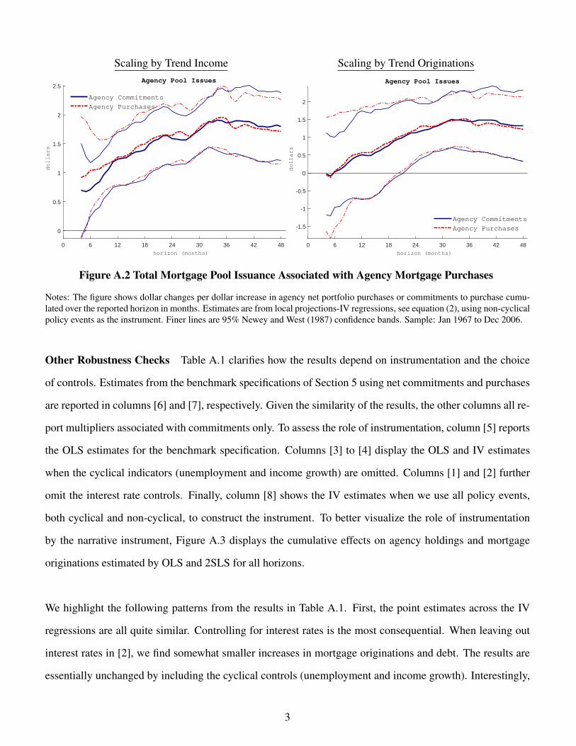
Scaling by Trend Income Scaling by Trend Originations

0 6 12 18 24 30 36 42 48horizon (months)

0

0.5

1

1.5

2

2.5

dollars

Agency Pool Issues

Agency Commitments

Agency Purchases

0 6 12 18 24 30 36 42 48horizon (months)

-1.5

-1

-0.5

0

0.5

1

1.5

2

dollars

Agency Pool Issues

Agency Commitments

Agency Purchases

Figure A.2 Total Mortgage Pool Issuance Associated with Agency Mortgage Purchases

Notes: The figure shows dollar changes per dollar increase in agency net portfolio purchases or commitments to purchase cumu-lated over the reported horizon in months. Estimates are from local projections-IV regressions, see equation (2), using non-cyclicalpolicy events as the instrument. Finer lines are 95% Newey and West (1987) confidence bands. Sample: Jan 1967 to Dec 2006.

Other Robustness Checks Table A.1 clarifies how the results depend on instrumentation and the choice

of controls. Estimates from the benchmark specifications of Section 5 using net commitments and purchases

are reported in columns [6] and [7], respectively. Given the similarity of the results, the other columns all re-

port multipliers associated with commitments only. To assess the role of instrumentation, column [5] reports

the OLS estimates for the benchmark specification. Columns [3] to [4] display the OLS and IV estimates

when the cyclical indicators (unemployment and income growth) are omitted. Columns [1] and [2] further

omit the interest rate controls. Finally, column [8] shows the IV estimates when we use all policy events,

both cyclical and non-cyclical, to construct the instrument. To better visualize the role of instrumentation

by the narrative instrument, Figure A.3 displays the cumulative effects on agency holdings and mortgage

originations estimated by OLS and 2SLS for all horizons.

We highlight the following patterns from the results in Table A.1. First, the point estimates across the IV

regressions are all quite similar. Controlling for interest rates is the most consequential. When leaving out

interest rates in [2], we find somewhat smaller increases in mortgage originations and debt. The results are

essentially unchanged by including the cyclical controls (unemployment and income growth). Interestingly,

3

and conditional on including the richest control set as in our benchmark specification, the results remain sim-

ilar when we also include the cyclically motivated policy events in the instrument, see column [8]. This is in

our view not too surprising. Based on our reading of the various historical policy actions, see Fieldhouse and

Mertens (2017), recognition and decision lags likely exceed one month in practice. With a sufficiently rich

set of lagged controls, including the cyclical actions may therefore not lead to any meaningful violation of

the exogeneity requirements. Instrumentation with policy events, however, is important for the results. The

OLS estimates in columns [1], [3], and [5] differ substantially in size and display very different time patterns

from the IV counterparts in columns [2], [4], and [6]: Agency holdings rise immediately and more or less

independently of the horizon, private holdings do not fall significantly over shorter horizons, and origina-

tions are higher by an amount that is much less dependent on the horizon. The OLS estimates are likely

contaminated by reverse causality, as this pattern is more consistent with private lenders simply passing on

newly originated loans to the agencies rather than selling existing loans off their balance sheets. Figure A.3

further illustrates this by depicting the full set of OLS and 2SLS estimates for agency holdings and mortgage

originations. Regardless of whether the baseline or full set of controls are included, the bulk of the increase

in mortgage originations per dollar change in commitments occurs within the first 12 months (panel A),

and within even a much shorter window when the regressor is agency purchases. Such a pattern indicates a

much stronger contemporaneous relation between originations and agency purchases. Given decision lags

as well as the time delays associated with the making of new mortgage loans, the delayed and gradual rise

in originations that appears after instrumentation is more consistent with a causal interpretation. Figure A.3

also reveals that the total agency mortgage holdings increase by a substantially smaller amount than the

dollar purchased or committed, even at relative short horizons. This indicates that agency purchases tend to

coincide with higher sales of mortgage assets to private investors and/or with higher repayment rates, both

of which are likely to reflect other influences on the private demand for mortgage credit in the primary or

secondary market.

Table A.2 verifies the robustness of the results to variations in the sample and to the inclusion of addi-

tional indicators of agency activity. For comparison, column [1] repeats the benchmark estimates based on

net commitments. For brevity, all other columns are based on using commitments as the measure of agency

4

purchasing activity. Column [2] extends the end point of the sample from December 2006 to December

2014. Note that in this case the h-th regression in (2) drops the last h observations. Column [3] restricts the

sample by setting September 1982 as the starting point, marking the end of the period of non-borrowed re-

serves targeting by the Federal Reserve. This shorter sample selects a period of more stable monetary policy.

Because of the smaller sample, we omit in this case the cyclical controls to reduce the number parameters to

be estimated. Columns [4], [5], and [6] show results when we omit in turn each of the three largest policy

interventions from the non-cyclical narrative instrument: the October 1977 conforming loan limit increase

and expansion of the Brooke-Cranston Tandem program, the December 1982 increase in Fannie Mae’s debt-

to-capital limit, and the September 2004 tightening of capital requirements. In each case we add the omitted

event as a separate dummy variable, including both the contemporaneous value and twelve lags to the con-

trol variables. The final two columns include lagged values of two indicators of agency activity as additional

controls: the volume of mortgage pool issues (in ratio of Xt) and log ratio of GSE stock prices to the S&P

500 index. In the latter case, the sample starts in September 1971 instead of December 1967, reflecting the

fact that Fannie Mae stock started trading on August 31, 1970.

All variations of the baseline specification reported in Table A.2 yield cumulative origination multipliers

in the range of 2.5 to 4.5 after 3 to 4 years. Moreover, the impact on originations is consistently highly

statistically significant. The estimated cumulative change in mortgage debt also remains in the range of the

benchmark specification. The credit multipliers are the lowest when we extend the sample to include the re-

cent financial crisis (column [2]) and when we add GSE excess stock returns to the control set (column [8]).

In these cases, the impact on mortgage debt is no longer significant at conventional levels. We also highlight

that the inclusion of the September 2004 policy event is important for the precision of the estimates. The

instrument that omits the 2004 event is generally weaker and produces wider confidence bands. On the other

hand, omitting the 1977 and 1982 events (columns [5] and [6]) does not have a large influence on the results.

5

A. Per Dollar in Agency Commitments

0 6 12 18 24 30 36 42 48horizon (months)

0

0.1

0.2

0.3

0.4

0.5

0.6

0.7

dollars

Agency Mortgage Holdings

2SLS with full controls

OLS with full controls

OLS with baseline controls

0 6 12 18 24 30 36 42 48horizon (months)

0

0.5

1

1.5

2

2.5

3

3.5

4

dollars

Mortgage Originations

2SLS with full controls

OLS with full controls

OLS with baseline controls

B. Per Dollar in Agency Purchases

0 6 12 18 24 30 36 42 48horizon (months)

0

0.1

0.2

0.3

0.4

0.5

0.6

0.7

0.8

0.9

dollars

Agency Mortgage Holdings

2SLS with full controls

OLS with full controls

OLS with baseline controls

0 6 12 18 24 30 36 42 48horizon (months)

0

0.5

1

1.5

2

2.5

3

3.5

4

dollars

Mortgage Originations

2SLS with full controls

OLS with full controls

OLS with baseline controls

Figure A.3 Comparing OLS and 2SLS Estimates of Mortgage Credit Multipliers

Notes: The figure shows dollar changes per dollar increase in agency net portfolio purchases or commitments to purchase cu-mulated over the reported horizon in months. The specification with baseline controls excludes the interest rate and cyclicalcontrols.

6

Table A.1 OLS and IV Estimates of Balance Sheet Adjustments and Mortgage Credit Multipliers

Months [1] [2] [3] [4] [5] [6] [7] [8]Agency Holdings 12 0.35∗∗∗ 0.61∗∗∗ 0.33∗∗∗ 0.68∗∗∗ 0.35∗∗∗ 0.66∗∗∗ 0.68∗∗∗ 0.56∗∗∗

(0.19,0.50) (0.35,0.88) (0.18,0.48) (0.43,0.93) (0.21,0.49) (0.40,0.92) (0.44,0.91) (0.25,0.87)

18 0.37∗∗∗ 0.55∗∗∗ 0.33∗∗∗ 0.58∗∗∗ 0.35∗∗∗ 0.54∗∗∗ 0.57∗∗∗ 0.42∗∗∗

(0.25,0.49) (0.33,0.78) (0.22,0.44) (0.35,0.81) (0.26,0.45) (0.30,0.77) (0.34,0.80) (0.15,0.70)

24 0.37∗∗∗ 0.50∗∗∗ 0.31∗∗∗ 0.51∗∗∗ 0.33∗∗∗ 0.47∗∗∗ 0.49∗∗∗ 0.37∗∗∗

(0.26,0.48) (0.29,0.71) (0.20,0.42) (0.29,0.73) (0.23,0.43) (0.26,0.69) (0.27,0.70) (0.12,0.63)

36 0.36∗∗∗ 0.26∗∗ 0.28∗∗∗ 0.26∗∗ 0.29∗∗∗ 0.23∗ 0.24∗ 0.15(0.27,0.46) (0.01,0.51) (0.18,0.38) (0.01,0.50) (0.20,0.38) (−0.00,0.47) (−0.01,0.50) (−0.15,0.44)

48 0.35∗∗∗ 0.25∗∗ 0.26∗∗∗ 0.23∗ 0.27∗∗∗ 0.22∗ 0.21∗ 0.19(0.25,0.44) (0.00,0.49) (0.16,0.36) (−0.03,0.49) (0.18,0.36) (−0.04,0.47) (−0.03,0.45) (−0.08,0.46)

Private Holdings 12 −0.16 −0.76∗∗ −0.12 −0.81∗∗ −0.11 −0.75∗∗ −0.77∗∗ −0.68∗

(−0.47,0.15) (−1.36,−0.15) (−0.40,0.15) (−1.43,−0.19) (−0.38,0.17) (−1.40,−0.11) (−1.39,−0.15) (−1.49,0.13)

18 −0.17 −0.43 −0.07 −0.31 −0.07 −0.23 −0.25 0.01(−0.41,0.06) (−1.01,0.15) (−0.29,0.14) (−0.94,0.31) (−0.28,0.14) (−0.81,0.34) (−0.86,0.36) (−0.70,0.73)

24 −0.12 −0.26 0.06 −0.11 0.06 −0.07 −0.07 0.20(−0.35,0.10) (−0.85,0.34) (−0.15,0.26) (−0.73,0.50) (−0.14,0.25) (−0.63,0.48) (−0.64,0.49) (−0.52,0.93)

36 −0.03 0.14 0.27∗∗∗ 0.34 0.30∗∗∗ 0.30 0.31 0.55(−0.29,0.22) (−0.73,1.01) (0.09,0.45) (−0.32,0.99) (0.11,0.49) (−0.27,0.88) (−0.28,0.91) (−0.17,1.27)

48 0.19 0.67 0.55∗∗∗ 0.90∗ 0.57∗∗∗ 0.82∗ 0.78∗ 0.84(−0.12,0.51) (−0.63,1.97) (0.32,0.78) (−0.14,1.94) (0.33,0.81) (−0.13,1.76) (−0.13,1.68) (−0.18,1.87)

Mortgage Debt 12 0.18∗∗ −0.14 0.21∗∗∗ −0.14 0.24∗∗∗ −0.09 −0.10 −0.12(0.02,0.35) (−0.54,0.26) (0.06,0.36) (−0.56,0.29) (0.09,0.40) (−0.53,0.34) (−0.54,0.34) (−0.70,0.46)

18 0.20∗∗∗ 0.12 0.26∗∗∗ 0.27 0.29∗∗∗ 0.30 0.32 0.44(0.06,0.34) (−0.31,0.56) (0.12,0.40) (−0.21,0.74) (0.14,0.43) (−0.11,0.72) (−0.13,0.77) (−0.10,0.97)

24 0.25∗∗∗ 0.24 0.37∗∗∗ 0.40∗ 0.39∗∗∗ 0.40∗ 0.41∗ 0.58∗∗

(0.10,0.39) (−0.23,0.71) (0.23,0.50) (−0.08,0.88) (0.25,0.53) (−0.01,0.81) (−0.02,0.84) (0.02,1.13)

36 0.33∗∗∗ 0.40 0.55∗∗∗ 0.59∗∗ 0.59∗∗∗ 0.54∗∗ 0.56∗∗∗ 0.70∗∗∗

(0.15,0.51) (−0.27,1.08) (0.43,0.68) (0.12,1.07) (0.46,0.73) (0.13,0.95) (0.14,0.98) (0.18,1.21)

48 0.54∗∗∗ 0.92∗ 0.81∗∗∗ 1.13∗∗∗ 0.84∗∗∗ 1.03∗∗∗ 0.98∗∗∗ 1.03∗∗

(0.30,0.78) (−0.16,1.99) (0.65,0.98) (0.31,1.95) (0.67,1.01) (0.31,1.76) (0.29,1.68) (0.24,1.83)

Originations 12 2.24∗∗∗ 1.33∗∗∗ 2.43∗∗∗ 1.22∗∗∗ 2.37∗∗∗ 1.32∗∗∗ 1.35∗∗∗ 1.45∗∗∗

(1.69,2.79) (0.42,2.24) (1.99,2.86) (0.37,2.07) (1.94,2.80) (0.44,2.20) (0.40,2.31) (0.41,2.50)

18 2.47∗∗∗ 1.87∗∗∗ 2.80∗∗∗ 2.00∗∗∗ 2.72∗∗∗ 2.14∗∗∗ 2.29∗∗∗ 2.50∗∗∗

(1.99,2.94) (0.99,2.74) (2.47,3.14) (1.14,2.85) (2.38,3.06) (1.32,2.96) (1.37,3.20) (1.55,3.45)

24 2.48∗∗∗ 2.03∗∗∗ 2.93∗∗∗ 2.37∗∗∗ 2.83∗∗∗ 2.52∗∗∗ 2.59∗∗∗ 2.94∗∗∗

(2.06,2.90) (1.17,2.89) (2.58,3.27) (1.49,3.26) (2.49,3.18) (1.68,3.35) (1.67,3.51) (1.92,3.97)

36 2.46∗∗∗ 2.83∗∗∗ 3.14∗∗∗ 3.38∗∗∗ 3.13∗∗∗ 3.40∗∗∗ 3.54∗∗∗ 3.62∗∗∗

(1.98,2.94) (1.39,4.28) (2.68,3.61) (2.00,4.77) (2.63,3.62) (2.10,4.71) (2.25,4.83) (2.15,5.10)

48 2.56∗∗∗ 3.38∗∗∗ 3.25∗∗∗ 4.02∗∗∗ 3.23∗∗∗ 3.96∗∗∗ 3.76∗∗∗ 3.92∗∗∗

(2.05,3.07) (1.34,5.41) (2.65,3.84) (2.13,5.90) (2.64,3.83) (2.20,5.72) (2.09,5.43) (2.02,5.82)

Dollar increase in: Comm. Comm. Comm. Comm. Comm. Comm. Purch. Comm.Method: OLS 2SLS-NC OLS 2SLS-NC OLS 2SLS-NC 2SLS-NC 2SLS-ALLInterest rate controls: No No Yes Yes Yes Yes Yes YesCyclical controls: No No No No Yes Yes Yes Yes

Notes: Numbers are dollar amounts. Estimates are from local projections-IV regressions, see equation (2). OLS: no instrumentused; 2SLS-NC, instrument based on non-cyclical policy events; 2SLS-ALL: instrument based on all policy events. 95% Neweyand West (1987) confidence bands in parentheses. Asterisks denote 10%, 5%, or 1% significance. Sample: Jan 1967 to Dec 2006.

7

Table A.2 Credit Multipliers, Sample and Robustness Checks

Months [1] [2] [3] [4] [5] [6] [7] [8]Agency Holdings 12 0.66∗∗∗ 0.76∗∗∗ 0.47∗∗∗ 0.88 0.64∗∗∗ 0.67∗∗∗ 0.72∗∗∗ 0.63∗∗∗

(0.40,0.92) (0.31,1.22) (0.23,0.71) (−0.35,2.11) (0.38,0.90) (0.38,0.96) (0.40,1.04) (0.32,0.94)

18 0.54∗∗∗ 0.62∗∗∗ 0.29∗∗∗ 0.78 0.52∗∗∗ 0.53∗∗∗ 0.60∗∗∗ 0.48∗∗∗

(0.30,0.77) (0.27,0.96) (0.12,0.46) (−0.18,1.75) (0.29,0.75) (0.27,0.78) (0.29,0.90) (0.12,0.85)

24 0.47∗∗∗ 0.55∗∗∗ 0.23∗∗ 0.59 0.45∗∗∗ 0.47∗∗∗ 0.53∗∗∗ 0.43∗∗

(0.26,0.69) (0.28,0.82) (0.05,0.42) (−0.16,1.35) (0.23,0.67) (0.24,0.69) (0.25,0.82) (0.04,0.81)

36 0.23∗ 0.32∗∗∗ −0.09 0.32 0.21 0.16 0.21 0.27(−0.00,0.47) (0.11,0.53) (−0.39,0.20) (−0.19,0.83) (−0.04,0.45) (−0.11,0.43) (−0.09,0.52) (−0.13,0.66)

48 0.22∗ 0.19 0.07 0.17 0.20 0.15 0.20 0.30(−0.04,0.47) (−0.10,0.47) (−0.30,0.44) (−0.82,1.16) (−0.07,0.46) (−0.15,0.44) (−0.14,0.54) (−0.08,0.68)

Private Holdings 12 −0.75∗∗ −1.23∗∗ −0.66∗ −0.83 −0.72∗∗ −0.83∗∗ −0.94∗∗ −0.95∗∗∗

(−1.40,−0.11) (−2.20,−0.27) (−1.33,0.00) (−3.34,1.68) (−1.36,−0.07) (−1.58,−0.08) (−1.70,−0.18) (−1.67,−0.23)

18 −0.23 −0.68∗ 0.05 0.31 −0.21 −0.32 −0.31 −0.30(−0.81,0.34) (−1.40,0.04) (−0.33,0.43) (−2.22,2.83) (−0.81,0.39) (−0.94,0.29) (−1.03,0.41) (−1.28,0.67)

24 −0.07 −0.53∗ 0.27 0.65 −0.04 −0.17 −0.11 −0.25(−0.63,0.48) (−1.15,0.09) (−0.10,0.64) (−1.76,3.07) (−0.62,0.54) (−0.73,0.38) (−0.82,0.60) (−1.30,0.80)

36 0.30 −0.24 0.87∗∗∗ 0.73 0.36 0.42 0.33 −0.24(−0.27,0.88) (−0.94,0.47) (0.37,1.36) (−0.47,1.93) (−0.24,0.97) (−0.27,1.11) (−0.40,1.05) (−1.05,0.57)

48 0.82∗ 0.41 1.27∗∗ 1.62 0.87∗ 1.09∗ 0.89 0.15(−0.13,1.76) (−0.79,1.61) (0.02,2.52) (−2.92,6.17) (−0.12,1.87) (−0.07,2.26) (−0.45,2.23) (−0.87,1.18)

Mortgage Debt 12 −0.09 −0.47 −0.19 0.05 −0.07 −0.16 −0.22 −0.32(−0.53,0.34) (−1.10,0.16) (−0.69,0.30) (−1.64,1.74) (−0.51,0.36) (−0.66,0.35) (−0.73,0.28) (−0.81,0.17)

18 0.30 −0.06 0.34∗ 1.09 0.31 0.20 0.29 0.18(−0.11,0.72) (−0.57,0.44) (−0.01,0.69) (−1.30,3.48) (−0.13,0.75) (−0.21,0.62) (−0.23,0.81) (−0.55,0.91)

24 0.40∗ 0.02 0.50∗∗∗ 1.25 0.41∗ 0.29 0.42 0.18(−0.01,0.81) (−0.46,0.49) (0.19,0.82) (−1.01,3.50) (−0.02,0.84) (−0.09,0.67) (−0.12,0.96) (−0.59,0.94)

36 0.54∗∗ 0.08 0.77∗∗∗ 1.05∗∗ 0.57∗∗∗ 0.58∗∗ 0.54∗∗ 0.03(0.13,0.95) (−0.54,0.70) (0.43,1.12) (0.06,2.03) (0.14,1.00) (0.09,1.06) (0.01,1.07) (−0.57,0.63)

48 1.03∗∗∗ 0.60 1.34∗∗∗ 1.79 1.07∗∗∗ 1.24∗∗∗ 1.09∗∗ 0.45(0.31,1.76) (−0.45,1.65) (0.40,2.29) (−1.87,5.46) (0.31,1.84) (0.33,2.15) (0.03,2.14) (−0.30,1.20)

Originations 12 1.32∗∗∗ 0.41 2.08∗∗∗ −0.23 1.39∗∗∗ 1.32∗∗∗ 1.14∗ 1.47∗∗∗

(0.44,2.20) (−1.47,2.28) (1.06,3.11) (−5.14,4.69) (0.51,2.26) (0.40,2.23) (−0.01,2.28) (0.48,2.46)

18 2.14∗∗∗ 1.40∗ 3.00∗∗∗ 1.56 2.20∗∗∗ 2.00∗∗∗ 2.04∗∗∗ 2.38∗∗∗

(1.32,2.96) (−0.02,2.83) (2.34,3.66) (−1.86,4.98) (1.38,3.03) (1.13,2.88) (0.88,3.20) (1.19,3.57)

24 2.52∗∗∗ 1.74∗∗∗ 3.61∗∗∗ 2.79∗ 2.59∗∗∗ 2.35∗∗∗ 2.55∗∗∗ 2.63∗∗∗

(1.68,3.35) (0.61,2.88) (2.95,4.28) (−0.21,5.79) (1.73,3.45) (1.48,3.22) (1.40,3.70) (1.05,4.20)

36 3.40∗∗∗ 2.51∗∗∗ 4.79∗∗∗ 4.43∗∗∗ 3.53∗∗∗ 3.56∗∗∗ 3.70∗∗∗ 2.69∗∗∗

(2.10,4.71) (1.27,3.75) (3.44,6.14) (1.29,7.57) (2.17,4.89) (2.00,5.12) (1.97,5.44) (0.92,4.46)

48 3.96∗∗∗ 3.39∗∗∗ 4.81∗∗∗ 5.59 4.07∗∗∗ 4.29∗∗∗ 4.35∗∗∗ 3.06∗∗∗

(2.20,5.72) (1.47,5.30) (2.22,7.40) (−2.41,13.60) (2.22,5.93) (2.13,6.45) (1.81,6.90) (1.23,4.89)

Sample: 67M1-06M12 67M1-14M12 82M10-06M12 67M1-06M12 67M1-06M12 67M1-06M12 67M1-06M12 71M09-06M12Modification: Benchmark Full Post-1982 Omitting Omitting Omitting Controls incl. Controls incl.

Sample Sample Sept 2004 Dec 1982 Oct 1977 Pool Issues GSE excess return

Notes: Numbers are dollar amounts. Estimates are from local projections-IV regressions, see equation (2), using non-cyclicalpolicy events as the instrument. 95% Newey and West (1987) confidence bands in parentheses. Asterisks denote 10%, 5%, or 1%significance.

8

A.2 Additional Results on Interest Rates and Credit Spreads

This section discusses a number of additional results regarding the effects of news shocks to agency pur-

chases on interest rates and credit spreads. Figure A.4 shows point estimates for the first 24 months after an

increase in anticipated purchases by one percentage point of trend originations, together with 95% Newey

and West (1987) confidence bands. The responses in blue are based on the regressions in (4) and the narrative

instrument. The responses in red are based on the regressions in (5) and the GSE excess returns instrument.

The first two panels in Figure A.4 show the responses of the AAA-rated and BAA-rated long term cor-

porate bond yields. Taken together, the results suggest that agency purchases exert a downward pressure on

corporate yields with a timing that coincides with the actual purchasing of mortgage assets by the agencies.

The response of the corporate yields is qualitatively similar to those of mortgage and Treasury rates, showing

initially no effect, and subsequently a gradual decline. The 95% confidence bands around the responses are

relatively wide, and the responses are only marginally significant in the case of the narrative instrument.

The declines in corporate bond yields are also quantitatively smaller than mortgage and Treasury rates, in

particular for the narrative instrument. The third panel in Figure A.4 shows statistically significant short-

run increases in the spread between AAA-rated corporate bonds and 10-year Treasuries. Agency purchases

appear therefore to induce the greatest spill-overs on the demand for the relative liquidity and safety of

Treasuries, which do not have prepayment risk. The increases are, however, relatively short-lived, with the

effects dissappearing after 7 or 8 months in the case of the narrative instrument, and only after a few months

in the case of the GSE excess returns instrument. The next panel shows evidence for a drop in the spread

between BAA and AAA-rated corporate bonds after 7 or 8 months, suggesting also some positive spill-over

effects on the demand for riskier long-term bonds.

The middle and right panels in the second row of Figure A.4 show declines in the spreads of mortgage

rates over the 10-year Treasure rates of a few basis points after about 6 months. The declines are at best

only marginally significant, indicating that agency purchases have important positive spill-over effects on

the demand for long-term Treasuries. The left panel in the bottom row of Figure A.4 shows the response of

the spread between the 3-month T-bill rate and the Federal Funds rate. With a delay of a few months, this

9

spread increases by 5 basis points or more when using the narrative instrument for identification. While this

may indicate some upward pressure on short-term interest rates relative to the funds rate target, the increase

is not statistically significant at conventional confidence levels. The GSE excess returns instrument does not

yield any indication of an impact. Finally, the right panel on the bottom row shows the response of the slope

of the Treasury yield curve, measured by the difference between the 10-year and 3-month yields. In the

case of the narrative instrument, there is initially no impact on the slope of the yield curve. However, as the

agency purchases induce a broad-based decline in both long and short-term interest rates, the slope of the

yield curve gradually steepens for the first 8 months. Subsequently, the yield curve flattens relatively quickly

and returns to prior levels one year after the new shock. In contrast, the GSE excess returns instrument does

not produce any significant impact on the slope of the Treasury yield curve.

10

Figure A.4 Impulses Responses to A Shock to Anticipated Agency Purchases

Notes: The figure shows responses to a one pp. increase in the expected future agency market share measured by agency com-mitments as a ratio of trend originations. Estimates are from local projections-IV regressions instrumented with the (1) narrativepolicy indicator, see equation (4), or orthogonalized GSE excess stock returns innovations, see equation (5). Finer lines and shadedareas are 95% Newey and West (1987) confidence bands. Sample: Jan 1967 to Dec 2006.

11

A.3 Impulse Responses of Mortgage Originations by Type

This section discusses additional results regarding the effects of news shocks to agency purchases on mort-

gage originations by type. The available data allows us to distinguish between refinancing and purchase

originations (see data appendix). The average share of refinancing originations in the 1967-2006 sample is

25% (and 28% in the 1967-2014 sample). The refinancing share is volatile and ranges from values of 10%

during the high nominal interest rates of the late 1970s and early 1980s, to up to 75% during refinancing

booms.

Figure A.5 shows point estimates for the first 24 months after an increase in anticipated purchases by one

percentage point of trend originations, together with 95% Newey and West (1987) confidence bands. The

responses in blue are based on the regressions in (4) and the narrative instrument. The responses in red are

based on the regressions in (5) and the GSE excess returns instrument. For reference, the left panel repeats

the responses of total mortgage originations shown in Figure 10. The middle panel shows the estimated

response of refinancing originations, while the right panel shows the estimated response of originations fi-

nancing the purchase of a home. We note that for the estimates in these two panels, the sample excludes

May 1985 to December 1986 because of missing data on refinance shares, see data appendix.

The results in Figure A.5 are consistent with those for the dollar credit multipliers reported in Section 5.

Refinancing originations show a gradual increase following the agency purchase shock, regardless of the in-

strument used for identification. Purchase originations also rise, but with a longer delay relative to refinance

originations. Using the narrative instrument, purchase originations are initially lower for the first six months

or so, before rising by similar levels between 12 and 24 months as for the GSE excess returns instrument. Us-

ing the average share of refinancing originations of 25% over the benchmark sample, the estimates in Figure

A.5 imply that refinancing originations account for the larger share of the increase in total originations.

12

Figure A.5 Impulse Responses to a Shock to Anticipated Agency Purchases

Notes: The figure shows responses to a one pp. increase in the expected future agency market share measured by agency commit-ments as a ratio of trend originations. Estimates are from local projections-IV regressions instrumented with the narrative policyindicator, see equation (4), or orthogonalized GSE excess stock returns innovations, see equation (5). Finer lines and shaded areasare 95% Newey and West (1987) confidence bands. Sample: Jan 1967 to Dec 2006. In the middle and right panels, the sampleexcludes May 1985 to Dec 1986 because of missing data on refinance shares, see data appendix.

Figure A.6 compares the response of originations to a traditional monetary policy shock (in red) with the

response to the agency purchase shock identified using the narrative instrument (in blue). Responses to

monetary shocks are identified using the Romer and Romer (2004) monetary policy shock measure as an

instrument, as explained in Section 7. As in Figure 13, the impact of the interest rate shock is scaled such

that the maximum decline in the 3-month T-bill rate is identical as for the agency purchase shock identified

with the narrative instrument. The left panel repeats the responses of total mortgage originations shown in

Figure 13 and shows that the agency purchase shock generates a larger increase in total originations. The

middle panel shows the responses of refinancing originations, while the right panel shows the estimated

responses of originations financing the purchase of a home. The results in Figure A.6 indicate that the

differential impact on total originations is due to the different impact on refinancing activity. The response

of purchase originations (right panel) is very similar in timing and size across both shocks. The response of

refinancing originations to monetary policy shock, on the other hand, is much more muted than the response

to the agency purchase shocks.

13

Figure A.6 Responses to A Shock to Anticipated Agency Purchases Versus a Monetary Policy Shock

Notes: The figure shows responses to a one pp. increase in the expected future agency market share as well as the response to amonetary policy shock. Estimates are from local projections-IV regressions instrumenting agency commitments with the narrativepolicy indicator, see equation (4), and instrumenting the 3 month T-Bill rate with the Romer and Romer (2004) monetary policyshock measure. Finer lines and shaded areas are 95% Newey and West (1987) confidence bands. Sample: Jan 1967 to Dec 2006.In the middle and right panels, the sample excludes May 1985 to Dec 1986 because of missing data on refinance shares, see dataappendix.

14

A.4 Impulse Response Analysis: Sensitivity Checks

Omitting the 1977-1982 and NBR-targeting Periods Figure A.7 shows the response to a shock to an-

ticipated agency purchases by one percentage point of trend originations, together with 95% Newey and

West (1987) confidence bands. Each figure shows results based on the narrative instrument for two differ-

ent subsamples. The first subsample omits the period of non-borrowed reserves targeting under the Volcker

chairmanship of the Federal Reserve from October 1979 to August 1982. The second subsample omits

the 6 years between 1977 and 1982, which are more broadly characterized by relatively high interest rate

volatility. Each of the excluded periods contain several sizeable credit policy changes as well as a greater

incidence of large monetary policy shocks in the Romer and Romer (2004) measure. Their exclusion allow

us to verify the role of these parts of the sample for our results regarding the interactions between the two

types of policies. The results in Figure A.7 are qualitatively very similar to those of the full sample, and in

both cases include both significant rise in originations as well as declines in short- and long-term interest

rates. Compared to the full sample, the rise in the stock of mortgage debt is, however, no longer evident

when we omit the 6 years between 1977 and 1982.

Post-1982 Sample Figure A.8 shows the response to a shock to anticipated agency purchases based on a

shorter sample that starts in October 1982 instead of December 1967. The Figure reports results for each

of the instruments, as in Figure 10. The October 1982 starting period marks the end of the period of non-

borrowed reserves targeting by the Federal Reserve and selects a period of more stable and inflation averse

monetary policy. Because of the smaller sample, we omit in this case the cyclical controls (personal income

and unemployment) to reduce the number parameters to be estimated. The results remain qualitatively very

similar to those of the full sample, indicating a rise in originations and declines in short- and long-term

interest rates. Compared to the full sample, the rise in the of stock mortgage debt is smaller and no longer

statistically significant in the case of the GSE excess returns instrument.

Omitting Policy Events from the Narrative Instrument Figure A.9 shows the response to a shock to

anticipated agency purchases for the benchmark specification together with those when we omit in turn

each of the three largest policy interventions from the narrative instrument: the October 1977 conforming

15

loan limit increase and expansion of the Brooke-Cranston Tandem program, the December 1982 increase

in Fannie Mae’s debt-to-capital limit, and the September 2004 tightening of capital requirements. In each

case we add the omitted event as a separate dummy variable, including both the contemporaneous value

and twelve lags to the control variables. While there is some variation in the size of the responses, the

results remain qualitatively similar to the benchmark narrative estimates. In all cases, there are increases in

originations and mortgage debt, and declines in short- and long-term interest rates.

Including Romer and Romer (2004) Shocks as Controls Figure A.10 compares the benchmark narrative

impulse response estimates of Figure 10 with those from a specification that includes both the contempo-

raneous value as well as 12 lags of the Romer and Romer (2004) monetary shock measure as additional

controls. Figure A.10 shows that controlling for the Romer and Romer (2004) shocks has little effect on the

estimation results.

16

Figure A.7 Impulse Responses Excluding 1977-1982 and NBR Targeting Periods

Notes: The figure shows responses to a one pp. increase in the expected future agency market share measured by agency commit-ments as a ratio of trend originations. Estimates are from local projections-IV regressions instrumented with the narrative policyindicator, see equation (4). Finer lines and shaded areas are 95% Newey and West (1987) confidence bands. Sample: Jan 1967 toDec 2006, excluding the period indicated.

17

Figure A.8 Impulses Responses in the Post-1982 Sample

Notes: The figure shows responses to a one pp. increase in the expected future agency market share measured by agency com-mitments as a ratio of trend originations. Estimates are from local projections-IV regressions instrumented with the (1) narrativepolicy indicator, see equation (4), or orthogonalized GSE excess stock returns innovations, see equation (5). Finer lines and shadedareas are 95% Newey and West (1987) confidence bands. Sample: Oct 1982 to Dec 2006.

18

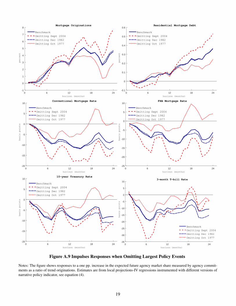
0 6 12 18 24horizon (months)

-1

0

1

2

3

4

5

6

7

8

percent

Mortgage Originations

Benchmark

Omitting Sept 2004

Omitting Dec 1982

Omitting Oct 1977

0 6 12 18 24horizon (months)

-0.1

0

0.1

0.2

0.3

0.4

0.5

0.6

percent

Residential Mortgage Debt

Benchmark

Omitting Sept 2004

Omitting Dec 1982

Omitting Oct 1977

0 6 12 18 24horizon (months)

-20

-15

-10

-5

0

5

10

basis points

Conventional Mortgage Rate

Benchmark

Omitting Sept 2004

Omitting Dec 1982

Omitting Oct 1977

0 6 12 18 24horizon (months)

-25

-20

-15

-10

-5

0

5

10

basis points

FHA Mortgage Rate

Benchmark

Omitting Sept 2004

Omitting Dec 1982

Omitting Oct 1977

0 6 12 18 24horizon (months)

-20

-15

-10

-5

0

5

10

basis points

10-year Treasury Rate

Benchmark

Omitting Sept 2004

Omitting Dec 1982

Omitting Oct 1977

0 6 12 18 24horizon (months)

-35

-30

-25

-20

-15

-10

-5

0

5

10

basis points

3-month T-bill Rate

Benchmark

Omitting Sept 2004

Omitting Dec 1982

Omitting Oct 1977

Figure A.9 Impulses Responses when Omitting Largest Policy Events

Notes: The figure shows responses to a one pp. increase in the expected future agency market share measured by agency commit-ments as a ratio of trend originations. Estimates are from local projections-IV regressions instrumented with different versions ofnarrative policy indicator, see equation (4).

19

Figure A.10 Controlling for Romer and Romer (2004) Shocks

Notes: The figure shows responses to a one pp. increase in the expected future agency market share measured by agency com-mitments as a ratio of trend originations. Benchmark estimates are from local projections-IV regressions instrumented with thenarrative policy indicator, see equation (4). The new specification includes additionally the contemporaneous value and 12 lags ofthe Romer and Romer (2004) shocks as controls. Finer lines and shaded areas are 95% Newey and West (1987) confidence bands.Sample: Jan 1967 to Dec 2006.

20

A.5 Forecast Error Contributions from an SVAR Model

The local projections-IV specifications do not allow an assessment of the historical role of structural shocks

to housing credit policy, which requires knowledge of the variance contribution of these shocks to the cumu-

lative purchase measures in equations (2) or (4). In order to gain some insight into the importance of GSE

activity for the dynamics of credit aggregates and interest rates, this section estimates the variance contri-

bution of the orthogonalized GSE excess returns innovations in a structural vector autoregressive (SVAR)

model. The main finding is that the contribution of GSE excess returns shocks to the short-run variability of

mortgage credit and housing starts is roughly as important as monetary policy shocks. In addition, shocks to

monetary policy are substantially more important for the forecast error variance of interest rates in the short

run. The role of GSE excess returns shocks for long-term interest rates exceeds the one of monetary policy

shocks at horizons beyond 18 months.

In order to estimate forecast error variance contribution of shocks to GSE activity, we adopt a VAR model

for the joint dynamics of the ratio of agency purchases and commitments to trend originations, as well as

all of the variables included as controls in the LPIV regressions: the log levels of core PCE and house price

indices, the log difference of total mortgage debt, the log levels of real mortgage originations and housing

starts, the 3-month T-bill rate, the 10-year Treasury rate, the conventional mortgage interest rate, the BAA-

AAA corporate bond spread, the unemployment rate, and the log of real personal income. In addition, the

VAR system also includes the log of the S&P 500 index and the log ratio of the GSE stock index to the S&P

500. We estimate the VAR by OLS using 12 lags of all the endogenous variables and using monthly data

from August 1971 to December 2006. The start of the sample reflects the month in which Fannie Mae stock

was traded for the first time on the New York Stock Exchange, which was August 1970.

The impact of a shock to orthogonalized GSE excess returns is the response to an innovation to the GSE stock

index variable, which is obtained by taking the lower triangular Choleski decomposition of the estimated co-

variance matrix of the VAR residuals, ordering all of the variables except agency purchases/commitments

above the GSE stock index variable. This approach imposes the same exclusion restrictions as the LPIV

model in (4) within the SVAR context, which amounts to assuming that none of the variables ordered before

21

the GSE stock index variable responds within the same month to orthogonalized GSE excess returns inno-

vations.

Figure A.11 shows the resulting impulse responses, which for ease of comparison are scaled to imply a

similar 6 month impact on originations as the LPIV estimates in Figure 10. The GSE excess returns shocks

lead to statistically significant increases in agency net commitments and net purchases (not shown). Con-

sistent with our main findings, Figure 10 shows that originations, mortgage debt and housing starts all rise

significantly following a positive innovations in GSE excess returns, while interest rates decline in the short

run. One difference between the VAR and the LPIV estimates in Figure 10 is that interest rates rise in the

longer run. The SVAR estimates are otherwise generally similar to those obtained using LPIV regressions

using the GSE excess returns as an instrument for agency mortgage purchases.

0 6 12 18 24horizon (months)

-6

-4

-2

0

2

4

6

8

percent

Mortgage Originations

0 6 12 18 24horizon (months)

-0.1

0

0.1

0.2

0.3

0.4

0.5

percent

Residential Mortgage Debt

0 6 12 18 24horizon (months)

-3

-2

-1

0

1

2

3

4percent

Housing Starts

0 6 12 18 24horizon (months)

-20

-15

-10

-5

0

5

10

15

20

25

30

basis points

Conventional Mortgage Rate

0 6 12 18 24horizon (months)

-20

-15

-10

-5

0

5

10

15

20

25

basis points

10-year Treasury Rate

0 6 12 18 24horizon (months)

-30

-20

-10

0

10

20

30

40

basis points

3-month T-bill Rate

Figure A.11 SVAR Impulse Responses to a GSE Excess Return Shock

Notes: The figure shows SVAR impulse responses to an innovation in orthogonalized GSE excess returns. Finer lines are 95%confidence bands obtained from a residual wild bootstrap using 10,000 replications. Sample: Aug 1970 to Dec 2006.

An advantage of the SVAR model is that it is straightforward to evaluate of the relative importance of shocks

22

in driving fluctuations in the endogenous variables. Figure A.12 depicts the share of the forecast error

variance at various horizons that is due to the identified GSE excess returns innovations. For comparison,

Figure A.12 also shows the variance contribution of monetary policy shocks identified using the Romer and

Romer (2004) measure as a proxy using the methodology in Stock and Watson (2012) and Mertens and

Ravn (2013). We find that the GSE excess returns shocks explain up to 9% of the agency net purchases

and commitments forecast variance (not shown). The contribution of monetary policy shocks remains below

2% at all horizons considered. Figure A.12 reveals that both shocks account for a substantial fraction of

the forecast variance of originations and housing starts at horizons beyond 6 months. GSE excess returns

shocks explain up to 14% of the forecast variance of originations at horizons between 12 and 18 months,

and around 7% to 8% of housing starts between 8 and 14 months. In comparison, monetary shocks explain

between 8% to 9% of originations, and around 14% of housing starts at similar horizons. Neither of the

shocks accounts for much of the forecast variance of the stock of mortgage debt at horizons up to 36 months.

Monetary shocks account for a substantial share of the short-run forecast variance of the 3-month T-bill

rates, and up to 11%, respectively 7%, of the variance in mortgage and 10-year Treasury rates at horizons

around 6 months. GSE excess returns shocks are relative less important for the variability in interest rates

at shorter horizons, but become relatively more important than monetary policy shocks in accounting for the

uncertainty in long-term interest rates at horizons exceeding 18 months.

23

0 6 12 18 24 30 36horizon (months)

0

5

10

15

percent

Mortgage Originations

GSE excess returns shock

Monetary shock

0 6 12 18 24 30 36horizon (months)

0

0.5

1

1.5

2

2.5

3

3.5

4

percent

Residential Mortgage Debt

GSE excess returns shock

Monetary shock

0 6 12 18 24 30 36horizon (months)

0

5

10

15

percent

Housing Starts

GSE excess returns shock

Monetary shock

0 6 12 18 24 30 36horizon (months)

0

2

4

6

8

10

12

percent

Conventional Mortgage Rate

GSE excess returns shock

Monetary shock

0 6 12 18 24 30 36horizon (months)

0

1

2

3

4

5

6

7

percent

10-year Treasury Rate

GSE excess returns shock

Monetary shock

0 6 12 18 24 30 36horizon (months)

0

5

10

15

20

25

30

35

40

45

percent

3-month T-bill Rate

GSE excess returns shock

Monetary shock

Figure A.12 Forecast Error Variance Contributions of Monetary and GSE Excess Returns Shocks

Notes: The figure shows contributions to the forecast error in the SVAR model. Monetary policy shocks are identified usingthe Romer and Romer (2004) measure as external instrument. GSE excess returns shocks are identified as described in the text.Sample: Aug 1970 to Dec 2006.

References

Mertens, Karel and Morten O. Ravn, “The Dynamic Effects of Personal and Corporate Income Tax Changesin the United States,” American Economic Review, 103 (2013), 1212–1247.

Romer, Christina D. and David H. Romer, “A New Measure of Monetary Shocks: Derivation and Implica-tions,” American Economic Review, 94 (2004), 1055–1084.

Stock, James H. and Mark W. Watson, “Disentangling the Channels of the 2007-2009 Recession,” BrookingsPapers on Economic Activity, 1 (2012), 81–135.

24