A Reconciliation of SVAR and Narrative

Estimates of Tax Multipliers∗

Karel Mertens and Morten O. Ravn

This draft: April 2012, first draft September 2011

Abstract

Existing empirical estimates of US nationwide tax multipliers vary from close to zero to

very large. Using narrative measures as proxies for structural shocks to total tax revenues in an

SVAR, we estimate tax multipliers at the higher end of the range: around two on impact and up

to three after 6 quarters. We show that earlier findings of lower multipliers can be explained by

an output elasticity of tax revenues assumption that is contradicted by empirical evidence or by

failure to account for measurement error in narrative series of tax shocks.

Keywords: Fiscal policy, tax changes, vector autoregressions, narrative identification, measure-

ment error

JEL Classification: E20, E32, E62, H30

∗We thank Matthieu Bussiere, Martin Eichenbaum, James Stock, Roberto Perotti and participants at various seminarsand conferences for useful comments. We also thank Jonas Fisher and Todd Walker for providing data. Mertens: De-partment of Economics, Cornell University, km426@cornell.edu; Ravn: Department of Economics, University CollegeLondon, m.ravn@ucl.ac.uk.

1 Introduction

The empirical literature on the dynamic output effects of unanticipated changes in tax policy does

not speak with one voice. Although most studies agree that tax increases are contractionary, there

is considerable disagreement regarding the size of the effect on economic activity. Estimates of tax

multipliers for the United States vary from close to zero to almost four, a range that is sufficiently

wide that the literature provides only limited guidance for theory and economic policy. The broad

range of estimates reflects numerous differences in methodology, including identification assump-

tions, model specifications, as well as sample coverage. In this paper, we use a new approach to

estimate tax multipliers associated with shocks to total federal tax revenues. Our estimates imply

tax multipliers of around two on impact and up to three after one-and-a-half years. Importantly, we

provide a reconciliation of our estimates with previous findings in the literature.

The main challenge to measuring the aggregate effects of changes in tax policy is endogeneity of

fiscal policy instruments. One strand of the literature has identified tax shocks by imposing short run

restrictions in structural vector autoregressions (SVARs). In a seminal contribution, Blanchard and

Perotti (2002) make assumptions on policy lags and calibrate certain parameters to identify struc-

tural innovations to taxes and government spending. Mountford and Uhlig (2009) use economic

theory to derive sign restrictions on VAR impulse responses. Another part of the literature instead

assumes that some exogenous changes in tax policy are observable. In a leading example, Romer

and Romer (2009) construct comprehensive narrative measures of legislated changes in federal tax

liabilities in the United States for the postwar period. A number of studies estimate the output effects

of tax changes as the response to innovations in one of these narrative measures.1

1Recent applications of the Blanchard and Perotti (2002) identification scheme to the estimation of tax multipliersinclude Ilzetzki (2011), Auerbach and Gorodnichenko (2012) and Caldara and Kamps (2012). Canova and Pappa (2007)adopt sign restrictions similar to Mountford and Uhlig (2009) to identify regional tax revenue shocks. The narrativeapproach to the estimation of tax multipliers has also been applied to other countries: for the UK, see Cloyne (2012);for a sample of OECD countries, see Favero, Giavazzi and Perego (2011).

1

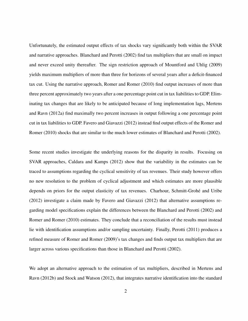
Unfortunately, the estimated output effects of tax shocks vary significantly both within the SVAR

and narrative approaches. Blanchard and Perotti (2002) find tax multipliers that are small on impact

and never exceed unity thereafter. The sign restriction approach of Mountford and Uhlig (2009)

yields maximum multipliers of more than three for horizons of several years after a deficit-financed

tax cut. Using the narrative approach, Romer and Romer (2010) find output increases of more than

three percent approximately two years after a one percentage point cut in tax liabilities to GDP. Elim-

inating tax changes that are likely to be anticipated because of long implementation lags, Mertens

and Ravn (2012a) find maximally two percent increases in output following a one percentage point

cut in tax liabilities to GDP. Favero and Giavazzi (2012) instead find output effects of the Romer and

Romer (2010) shocks that are similar to the much lower estimates of Blanchard and Perotti (2002).

Some recent studies investigate the underlying reasons for the disparity in results. Focusing on

SVAR approaches, Caldara and Kamps (2012) show that the variability in the estimates can be

traced to assumptions regarding the cyclical sensitivity of tax revenues. Their study however offers

no new resolution to the problem of cyclical adjustment and which estimates are more plausible

depends on priors for the output elasticity of tax revenues. Charhour, Schmitt-Grohe and Uribe

(2012) investigate a claim made by Favero and Giavazzi (2012) that alternative assumptions re-

garding model specifications explain the differences between the Blanchard and Perotti (2002) and

Romer and Romer (2010) estimates. They conclude that a reconciliation of the results must instead

lie with identification assumptions and/or sampling uncertainty. Finally, Perotti (2011) produces a

refined measure of Romer and Romer (2009)’s tax changes and finds output tax multipliers that are

larger across various specifications than those in Blanchard and Perotti (2002).

We adopt an alternative approach to the estimation of tax multipliers, described in Mertens and

Ravn (2012b) and Stock and Watson (2012), that integrates narrative identification into the standard

2

SVAR framework.2 The key identifying assumptions are that the narrative measures correlate with

tax shocks but are orthogonal to other structural shocks. The narrative tax changes are treated as

proxy measures of latent structural tax shocks, which is why we refer to it as the ‘proxy SVAR’

approach. The main idea is to complement the usual VAR residual covariance restrictions with mo-

ment restrictions on the proxy to achieve identification. An application to US post WWII data yields

estimates of tax multipliers that are large, robust and relatively precisely estimated. At medium

forecast horizons, our results support tax multipliers at the higher end of the range, such as those of

Mountford and Uhlig (2009) and Romer and Romer (2010). However, we find tax multipliers that

are larger than these studies also in the short run.

The proxy SVAR allows us to elicit the underlying differences between the estimates produced

by alternative identification schemes. Unlike the Blanchard-Perotti SVAR, the proxy SVAR does

not require direct assumptions on key structural elasticities but instead estimates them. Because the

specification in both SVARs are identical in every other respect, the discrepancy between results can

be traced to the values of those structural elasticities. The answer lies exclusively with the output

elasticity of tax revenues. The proxy SVAR estimates this elasticity to be high and rejects at the 95

percent level the lower cyclical elasticities calculated by international organizations on which Blan-

chard and Perotti (2002) rely. We provide several criticisms of the conventional cyclical adjustment

procedures and argue that alternative methods available in the literature, while small in number, all

point to high output elasticities, and therefore large tax multipliers.

Our methodology also has an advantage over existing narrative approaches because it is robust to

various types of measurement error. We discuss several reasons why some error in measurement is

hard to avoid when constructing the narrative measures of tax shocks, including those that concern

2The identification approach was outlined earlier for SVARs in an NBER lecture by Stock and Watson (2008). Stockand Watson (2012) apply the methodology to dynamic factor models for the identification of a wide range of shocks.

3

Perotti (2011). The proxy SVAR yields estimates of the statistical reliability of the narrative series,

which measures the squared correlation between the narrative measures and the estimated structural

shocks. This statistic allows for an evaluation of the quality of different available tax shock mea-

sures. We find for instance that it is important to correct for anticipated tax changes. Another issue

in the calculation of the output effects of tax changes is the scaling of shocks. As in Blanchard and

Perotti (2002) or Mountford and Uhlig (2009), we scale the tax shocks by their impact on tax rev-

enues to obtain tax multipliers. Standard applications of the narrative approach instead scale the tax

shocks in terms of their projected impact on tax liabilities. We quantify the measurement error bias

present in the existing narrative specifications through simulations. We find that measurement error

explains the differences across the narrative estimates and is the reason for the low tax multipliers

estimated by Favero and Giavazzi (2012).

The key objective of this paper is to understand the dispersion of estimated tax multipliers associated

with unanticipated shocks to total revenues. In doing so, we abstract from other issues relevant to

the empirical characterization of the aggregate effects of tax policy shocks. For instance, we focus

exclusively on unanticipated tax changes. Other studies have looked at shocks to expectations of

future tax policy, e.g. Mountford and Uhlig (2009), Mertens and Ravn (2012a), Leeper, Walker and

Yang (2011) or Kueng (2011). As in most previous work, there is no attempt to define more narrowly

which of the many tax instruments is adjusted, as is done in Barro and Redlick (2011) or Mertens

and Ravn (2012b). Finally, we restrict attention to linear models that do not allow for time-varying

effects as in Auerbach and Gorodnichenko (2012). Nonetheless, the identification and measurement

issues we raise are also highly relevant for extensions in any of these directions.

4

2 Empirical Models

The first step of our analysis is to replicate existing results on the output effects of tax shocks for

the same dataset. We focus on the SVAR of Blanchard and Perotti (2002) and several narrative

specifications and contrast the results with those from our new empirical model, the proxy SVAR.

2 .1 The SVAR of Blanchard and Perotti

The benchmark application of Blanchard and Perotti’s (2002) methodology estimates the impact of

discretionary tax shocks from a VAR using data on total tax revenues Tt , government spending Gt

and output Yt . The dynamics of the observables Zt = [Tt ,Gt ,Yt ]′ are modeled by a VAR,

Zt = α′dt +δ′Zt−1 +Bεt , (1)

where dt contains deterministic terms with coefficients α, Zt−1 = [Z′t−1, ...,Z

′t−p]

′ is the vector of

lagged observables, p is the number of lags, δ is a matrix of autoregressive coefficients, B is a

nonsingular matrix of coefficients, and εt = [εTt ,εG

t ,εYt ]

′ is a vector of structural shocks with E[εt ] =

0, E[εtε′t ] = I, E[εtε′s] = 0 for s = t. Let ut = [uTt ,u

Gt ,u

Yt ]

′ denote the reduced form residuals, which

are by assumption linearly related to the structural shocks:

ut = Bεt . (2)

Estimates of α, δ and E[utu′t ] are straightforward to obtain by for instance OLS but the structural

coefficients B and shocks εt are not identified. The requirement that E[utu′t ] = BB ′ provides six

independent identifying restrictions. Obtaining all nine elements of B requires at least three more

5

identifying restrictions. Without loss of generality, we can express the reduced form errors as:

uTt = θGσGεG

t +θY uYt +σT εT

t ,

uGt = γT σT εT

t + γY uYt +σGεG

t , (3)

uYt = ζT uT

t +ζGuGt +σY εY

t .

The parameters θY and γY measure the cyclical elasticities of tax revenues and spending respectively;

θG and γT capture the interdependence between fiscal instruments; and ζT and ζG parametrize the

contemporaneous dependence of economic activity on fiscal policy. The remaining parameters are

the standard deviations of all sources of exogenous variation in the variables.

The identification strategy proposed by Blanchard and Perotti (2002) is based on restricting the

values of the contemporaneous responses of government spending to tax shocks, γT , and cyclical

output movements, γY , as well as the elasticity of tax revenues to output, θY . Based on the assump-

tion of decision and recognition lags in fiscal policy, the parameters γT and γY are restricted to zero.

The output elasticity of tax revenues θY is instead calibrated to an outside estimate of the cyclical

sensitivity of revenues. Blanchard and Perotti (2002) adopt the OECD methodology described in

Giorno et al. (1995) to obtain a value for θY . Fixing the values of these parameters provides the

three independent restrictions required to identify structural impulse responses.

We reproduce the results of Blanchard and Perotti (2002) using data from the BEA’s NIPA tables on

federal tax revenues, federal government consumption and investment expenditures and output, all

in log real per capita terms and for the sample 1950Q1 to 2006Q4.3 All VAR specifications have

3Output is GDP in line 1 from Table 1.1.5; government spending is Federal Government Consumption Expendituresand Gross Investment in line 6 from Table 3.9.5; Total tax revenue is Federal Current Tax Receipts in line 2 of Table3.2 and Contributions for Government Social Insurance in line 11 of Table 3.2 less corporate income taxes from FederalReserve Banks (line 8 in Table 3.2). All series are deflated by the GDP deflator in line 1 from Table 1.1.9 and by thecivilian population ages 16+ obtained from Francis and Ramey (2009). The NIPA data was last revised July 29, 2011.

6

four lags of the endogenous variables and, as in Blanchard and Perotti (2002), include a constant,

linear and quadratic trends and a dummy for 1975Q2. Because our goal is to compare results with

the narrative estimates of the output response to federal tax changes recorded by Romer and Romer

(2009), we use data at the level of the federal instead of the general government as in Blanchard and

Perotti (2002). We use the original value for θY used in Blanchard and Perotti (2002) of 2.08, even

though the latter pertains to the elasticity of general government revenues.4

The impulse responses of output we report have the interpretation of tax multipliers, i.e. dollar

changes in GDP as a ratio of the dollar changes in tax revenues. In the Blanchard-Perotti SVAR,

these are obtained by dividing the response to a tax revenue shock of minus one percent by the aver-

age ratio of federal tax revenues to GDP in the sample of 17.5%. Equivalently, the numbers reflect

the percent response to a tax cut that lowers tax revenues by one percentage point of GDP. Unless

mentioned otherwise, we provide 95% confidence intervals that are computed using a recursive wild

bootstrap using 10,000 replications, see Goncalves and Kilian (2004).5

Panel (A) of Figure 1 presents the effect on output of an exogenous tax cut in the Blanchard-Perotti

SVAR. On impact, output increases by 0.48 percent in response to the tax shock, whereas the max-

imum output effect of 1.35 percent occurs after two years. The output increase is significantly

different from zero at the 95% level for the first three years after the shock. Despite the differences

in data definitions and sample coverage, these estimates are similar to the estimated impact and peak

multiplier of 0.69 and 0.78, respectively, in the original paper by Blanchard and Perotti (2002). The

first column of Table 1 lists the underlying estimates of the parameters of the system in (3).

4Using a variation of the same methodology, Follette and Lutz (2010) provide an estimate of the output elasticity oftax revenues θY of 1.6 for the US at federal level. However this estimate is based on annual data.

5In the application of the wild bootstrap, we multiply in each artificial sample every ut with a random variable takingon values of -1 or 1 with probability 0.5.

7

2 .2 Standard Narrative Approaches

A leading alternative identification strategy for estimating the dynamic effects of tax shocks is based

on the narrative approach. Romer and Romer (2009) construct measures of exogenous changes

in taxes from a variety of government sources by recording the (projected) impact on federal tax

liabilities of legislated tax code changes. Their selection of exogenous changes in tax liabilities is

based on a classification of the motivation for the tax change either as ideological or as arising from

inherited debt concerns. Romer and Romer (2010) estimate the output response to changes in taxes

from a univariate regression for output growth

∆Yt = α′dt +λ0τt +λ1τt−1 + ...+λkτt−k +wt , (Romer and Romer (2010))

where dt are deterministic terms, τt are the narrative shocks to total tax liabilities as a percentage of

GDP and the λ′s are slope coefficients. If τt and its k lags are exogenous, i.e. uncorrelated with the

residual wt , then OLS estimates of the λ’s are structural impulse response coefficients to innovations

in the measured tax changes τt . One can view the equation in terms of a moving average (or Wold)

representation of ∆Yt in which wt captures the effects of contemporaneous and lagged realizations

of structural shocks other than those observed directly by τt . The required exogeneity assumption is

therefore that the τ’s are uncorrelated with all current and past realizations of these other shocks.

There are several possible reasons why the measure for tax shocks used by Romer and Romer (2010)

may fail to satisfy the necessary exogeneity assumptions. The first is that a subset of the tax interven-

tions are motivated as responses to inherited deficits. In practice however, several studies, including

Romer and Romer (2010), Mertens and Ravn (2012a) and Favero and Giavazzi (2012), all fail to

reject the hypothesis that the occurrence or size of the Romer and Romer (2010) tax changes are

unpredictable by past observations of macroeconomic aggregates. Another key issue is that many

changes in the tax code are legislated well in advance of scheduled implementation. In Mertens and

8

Ravn (2012a) we disaggregate the tax shock series into unanticipated and anticipated tax changes

on the basis of the implementation lag and find evidence for macroeconomic effects of legislated tax

shocks prior to their implementation. These preannounced tax changes thus reflect past tax ‘news’

shocks rather than surprise current tax changes which leads to a violation of the exogeneity require-

ment.6 For this reason, here we only use those exogenous tax changes for which the legislation and

implementation date are less than one quarter apart. The narrative measure τt for tax shocks is ob-

tained by dividing the unanticipated changes in tax liabilities by previous quarter nominal GDP. In

total, τt has 26 nonzero observations and the series is depicted in Figure 2. We estimate the Romer

and Romer (2010) regression of output growth on a distributed lag of τt with k = 12 and a constant

as the only deterministic term.

We also present estimates of the tax multipliers derived from two alternative empirical specifica-

tions used in the literature,

Zt = α′dt +δ′Zt−1 +λ0τt + vt , (Favero and Giavazzi (2012))

Zt = α′dt +δ′Zt−1 +λ0τt +λ1τt−1 + ...+λkτt−k + vt , (Mertens and Ravn (2012a))

The specifications of Favero and Giavazzi (2012) and Mertens and Ravn (2012a) are vector autore-

gressions augmented with the contemporaneous value or a distributed lag of τt . In the latter, we set

k = 12. Both these specifications include the same deterministic terms and autoregressive lags as

the Blanchard-Perotti SVAR. The dynamic effects of tax shocks are obtained in each specification

by tracing out the responses to a shock to τt . Both these specifications rely on the same exogeneity

assumptions as the univariate regression.

6Changing the timing of the anticipated tax changes to the announcement date and combining them with the unan-ticipated tax changes is inappropriate since we find they have very different effects on output. We find no evidence formacroeconomic effects prior to those tax changes that we classify as unanticipated.

9

The estimates of the output effects of tax changes in all three narrative specifications differ from

those of the Blanchard-Perotti SVAR because of the different identification strategy and because of

differences in the reduced form transmission mechanism. Given the variations in time series specifi-

cations, heterogeneity in the narrative estimates is to be expected because of the differential impact

of small sample uncertainty and/or model misspecifications. A more subtle issue regards the scaling

of the tax shocks. In the Blanchard-Perotti SVAR, the tax shocks are scaled by their impact on ac-

tual tax revenues while the narrative studies scale the response by the impact on τt , i.e. the projected

impact on tax liabilities assuming no change in the tax base.

Panels (B), (C) and (D) of Figure 1 depict the output responses for each model to a one percentage

point shock to τt . The Romer and Mertens-Ravn specifications, both of which include multiple lags

of the tax narrative, find impact effects on output that are only slightly higher than the Blanchard-

Perotti SVAR estimates of the impact multipliers: 0.78 and 0.73 respectively. The maximum output

effects, however, are instead substantially larger: 2.96 percent in the 10th quarter for the Romer spec-

ification and 2.34 percent in the eight quarter for the Mertens-Ravn specification. The confidence

intervals associated with these estimates are relatively wide and easily contain the Blanchard-Perotti

SVAR point estimates. The responses in the Favero-Giavazzi model are instead much closer to the

Blanchard-Perotti SVAR at all horizons: the impact effect on output is 0.77 percent, but the out-

put response never exceeds 1.17 percent. The output effects are more precisely estimated by the

Favero-Giavazzi model because of a more parsimonious parametrization in the tax shocks. Despite

the differences in the data used, the results are very similar to those of the original papers.

2 .3 The Proxy SVAR

We now present an alternative approach to estimating the impact of a tax shock: the proxy SVAR,

which integrates the narrative identification approach into the standard SVAR framework. The proxy

SVAR in this section is a straightforward application of the methodology described in Mertens and

10

Ravn (2012b) and Stock and Watson (2012). Unlike the standard narrative estimates of the tax mul-

tipliers, impulse responses in the proxy SVAR are based on the same VAR as the Blanchard-Perotti

approach, see equations (1)-(2). However, instead of directly assuming certain values for the coeffi-

cients underlying the elements of the impact matrix B , it exploits the informative content of narrative

series of policy changes by using these as proxy measures mt for the latent structural tax shock εTt .

Without loss of generality, assume that E[mt ] = 0. The proxy variable mt must satisfy

E[mtεTt ] = ϕ = 0 , (4)

E[mtεGt ] = 0 , E[mtεY

t ] = 0 . (5)

The first condition states that the proxy is contemporaneously correlated with the structural tax

shock. The second condition requires the proxy to be uncorrelated with contemporaneous spending

and output shocks. When these conditions hold, the proxy variable can be used for identification

of the structural tax shock and the associated impulse response function. As the proxy variable for

latent tax revenue shocks, we use the narrative series τt after removing the mean from the nonzero

observations (the mean is approximately zero). Note that these identifying assumptions are weaker

than those required in the standard narrative specifications. First, the proxy variable must have a

nonzero correlation with the structural tax revenue shock, but the correlation does not need to be

perfect. This means that τt does not have to contain fully accurate observations of the tax shock.

Second, it is not required that mt is uncorrelated with past structural shocks.

Implementing the identifying restrictions is straightforward. Let βT denote the (first) column of

the impact matrix B associated with the tax shock εTt . The conditions in (4)-(5) imply that

ϕβT = E[utmt ] (6)

11

This condition states that the covariance between the reduced form VAR residuals and the proxy

mt is proportional to βT . Because the extent of the correlation between the proxy mt and εTt is

unknown, the constant of proportionality ϕ is unknown. Nonetheless, condition (6) provides two

additional independent restrictions that suffice to trace out the response to a tax shock of any given

size. In practice, the tax multipliers are easily obtained by (1) estimating the reduced form VAR, (2)

regressing the reduced form residuals on the proxy variable mt and (3) rescaling the response func-

tions as in the Blanchard-Perotti SVAR to generate the intended effect on tax revenues. Restrictions

such as (6) are always equivalent to an instrumental variables procedure, see Hausman and Taylor

(1983). In this case one can alternatively view assumptions (4)-(5) as instrument validity conditions

in 2SLS regressions of uGt and uY

t on uTt using mt as the instrument.7

Figure 3 depicts the nonzero observations of the proxy variable against the corresponding structural

tax shocks identified by the proxy SVAR. There is a visible positive relationship and the R squared of

the associated regression line is 0.34. In Section 4 below, we will quantify the relationship between

the shocks and various proxy variables using an asymptotically equivalent reliability statistic. Figure

4 presents the impulse responses of output, spending and tax revenues to an exogenous decrease in

taxes, together with the 95% confidence bootstrap intervals.8 In response to a shock to tax revenues

of one percentage point of GDP, output increases by 2.00 percent on impact and rises to a maximum

of almost 3.19 percent above trend after 5 quarters, before subsequently reverting to trend. Hence, at

longer forecast horizons, the proxy SVAR predicts output effects that are relatively large and more

in line with the results of the Romer/ Mertens-Ravn specifications than the Blanchard-Perotti and

Favero-Giavazzi specifications. However, the proxy SVAR also finds substantially larger short run

7See Stock and Watson (2008) for the IV interpretation. Mertens and Ravn (2012b) discuss a case with n correlatedproxies for n shocks. Stock and Watson (2012) consider cases with multiple proxies (’external instruments’) for onestructural shock.

8In the application of the wild bootstrap, we multiply in each artificial sample every ut and mt with a randomvariable taking on values of -1 or 1 with probability 0.5. Thus, the bootstrap inference procedure also takes into accountuncertainty about identification and measurement.

12

effects of tax shocks than any of the other specifications. In particular, the confidence regions of the

Blanchard-Perotti and proxy SVARs do not overlap for the first few quarters after the tax decrease,

such that the differences across SVAR identification schemes are statistically significant.

The finding that the proxy SVAR uncovers large tax multipliers is very robust. In Mertens and

Ravn (2012b), we use the same methodology to estimate the separate effects of personal and corpo-

rate income taxes based on a new narrative dataset and find similarly large output effects of cuts to

either tax type. Before we make the case in favor of the larger estimates for the tax multipliers, we

first examine the robustness of the finding in the context of shocks to total tax revenues:

Alternative Narrative Measures Panel (A) of Figure 5 depicts the estimated output responses

when we use a few alternative versions of the unanticipated Romer and Romer (2009) exogenous

tax shock series: one that excludes all tax changes that were motivated due to inherited budget

concerns (‘Long run growth only’), one that takes into account any retroactive provisions of the

legislated changes (‘Retroactive’), and a series for which the tax liabilities are scaled by previous

year GDP instead of previous quarter GDP (‘Scaled by Yt−4’). None of these alternative narrative

series for unanticipated tax shocks have much effect on the tax multiplier estimates.

Trend Assumptions The SVAR multiplier estimates of Blanchard and Perotti (2002) are some-

what sensitive to assumptions about trends. Panel (B) of Figure 5 shows the tax multipliers in the

proxy SVAR when we switch to a stochastic trend assumption by including all variables in first

differences. The main consequence is that the effect of a tax shock on output becomes permanent,

with an associated long run multiplier of 3.39. However, the trend assumptions make very little

difference for the point estimates for at least the first two years after the shock.

Fiscal Foresight To comply with the exogeneity assumptions required for the standard narrative

approaches, we used a tax shock measure that omits all tax liability changes that were implemented

13

more than 90 days after becoming law. Because in the proxy SVAR a zero correlation between the

narrative measure and past shocks is not a requirement, the omission of tax changes that are likely to

be correlated with past tax news shocks is not strictly necessary. However, this apparent advantage

of the proxy SVAR is subject to two potential caveats.

The first is that the proxy SVAR also relies on the assumption that the VAR prediction errors are lin-

early related to the contemporaneous structural shocks, see equation (2). Several recent papers have

shown that in the presence of anticipated fiscal shocks, the traditional set of conditioning variables

may not contain sufficient information to satisfy this assumption.9 We address this issue by ex-

panding the conditioning set with variables that plausibly contain independent information on fiscal

expectations. We add as a fourth endogenous variable, in turn: a measure of expected future taxes

that is implied by tax exempt municipal bond yields and perfect arbitrage, constructed by Leeper et

al. (2011), (‘Implicit tax rate’); a defense sector stock returns variable, which is a series for the ac-

cumulated excess returns of large US military contractors constructed by Fisher and Peters (2010),

(‘Defense returns’); and Ramey’s (2011) defense spending news variable, which contains profes-

sional forecasters’ projections of the path of future military spending, (‘Defense News’).10 Panel

(C) of Figure 5 shows that including these variables has no notable effects on the estimates.

The second potential caveat is that to obtain accurate results in small samples, it is important that

the correlation between the proxy and the latent unanticipated tax shock is sufficiently large. This

means that good proxies of unanticipated tax shocks should have minimal predictable variation un-

related to surprise tax changes. We investigate the results for several other proxies that may differ in

9Leeper, Walker and Yang (2011) show that the omission of important variables can potentially produce misleadingresults when agents have foresight about future taxes. Ramey (2011) similarly questions the identifiability of shocks inthe Blanchard-Perotti VAR in the presence of foresight about government spending.

10We use Leeper, Walker and Yang (2011)’s implicit tax rate variable based on bonds with maturity of one year. Sincethis data is only available since 1953Q2, the sample was shortened correspondingly in this case.

14

this dimension. In Panel (D), we use as the proxy variable the error in a regression of the (nonzero

observations) of the tax narrative on four lags of the Leeper et al. (2011) implicit expected tax rate

implied by municipal bond spreads. The idea is to remove any remaining predictable components of

the tax narrative used in the benchmark specification.11 We find that municipal bond spreads have

little predictive power for tax changes we classified as unanticipated and the estimated tax multipli-

ers remain close to the benchmark estimates. In Panel (E) of Figure 5 we instead use the original

Romer series for exogenous tax changes. This leads to substantially lower multipliers and the point

estimates are in fact very close to those of the Blanchard-Perotti SVAR in Panel (A) of Figure 1. The

original Romer measure does not eliminate legislative changes with implementation lags exceeding

one quarter, adding 19 observations to the proxy that we used in the benchmark.12 The sensitivity

to the inclusion of preannounced tax changes almost certainly reflects a decrease in the quality of

the proxy as a measure of unanticipated shocks. A first clear indication is that a straightforward ad-

justment to the Romer series for expectations about future taxes almost fully restores the estimates

of the benchmark proxy SVAR. In Panel (F) of Figure 5, we still use all implemented tax changes in

the Romer series to construct the proxy. However, we first regress the anticipated changes on lagged

observations of the Leeper et al. (2011) expected future tax rate series to eliminate the predictable

component. We then merge the error in this regression with the unanticipated shocks to construct an

anticipation adjusted proxy for tax shock innovations. The resulting output response is close to the

benchmark proxy SVAR that used only the subset of unanticipated shocks. It turns out that, unlike

the tax changes we classified as unanticipated, the anticipated tax changes are to a large extent pre-

dicted by municipal bonds spreads, such that the additional observations contain very little genuine

information about unanticipated variation in taxes. In Section 4 below, we provide more formal

evidence for this claim by comparing estimates of the statistical reliability of the various proxies.

11See Kueng (2011) for recent evidence of the predictive power of municipal bond spreads for tax rates.12There are 24 observations of preannounced tax changes in the sample, but 5 occur in a quarter where there is also

an unanticipated tax change observation.

15

3 Reconciling the SVAR Estimates of Tax Multipliers

Applying the different methodologies to the same dataset yields estimates of output responses to tax

shocks that are representative for the very broad range found in the literature. We begin by isolating

the reason for the difference between Blanchard and Perotti’s (2002) relatively small tax multipliers

and those obtained from the proxy SVAR.

3 .1 Understanding the Difference

The key feature of the proxy SVAR that makes a comparison straightforward is that, unlike the

other narrative approaches, it has the same estimated reduced form transmission mechanism as the

Blanchard-Perotti SVAR. Therefore, the discrepancy in tax multipliers must be apparent in the struc-

tural parameters of the contemporaneous impact matrix B . The conditions in (4) -(5) exploited by

the proxy SVAR implies two independent restrictions on B . Whereas these are sufficient to derive

the impulse response function associated with tax shocks, to identify all the parameters of the sys-

tem in (3) in the proxy SVAR, we need one additional restriction. Of the three parameter restrictions

imposed by Blanchard and Perotti (2002), we adopt the assumption that government spending does

not react contemporaneously to changes in economic activity, i.e. γY = 0. This assumption can be

motivated by the presence of decision and recognition lags and seems in our view the least question-

able.13 Consequently, the discrepancy in results must manifest itself either in the value of the output

elasticity of tax shocks θY , the elasticity of spending to tax policy shocks γT , or both.

The first two columns of Table 1 provide the estimates for the structural parameters in both SVAR

specifications together with 95% confidence intervals. The main result is that the proxy SVAR

strongly rejects the calibrated value for the output elasticity of tax revenues, θY = 2.08, assumed

in the Blanchard-Perotti SVAR. The point estimate for θY is 3.13 with 95% percentiles of 2.73 and

13Assuming alternatively that γT = 0 in the proxy SVAR leads to the same conclusions.

16

3.55. The other testable assumption of the Blanchard-Perotti SVAR is the absence of a within quar-

ter response of government spending to tax shocks, i.e. γT = 0. The point estimate for γT is 0.06

with 95% percentiles of −0.06 and 0.17. Thus, this assumption is not contradicted by the proxy

SVAR. The other structural elasticities are all relatively similar across identification schemes, and

the remaining differences are mainly reflected in the standard deviations of the shocks. The finding

that the narrative identification strategy implies a higher cyclical sensitivity of tax revenues is robust

to the use of alternative tax shock measures. The first column of Table 2 lists the estimated values for

θY for different proxies. The point estimates for the elasticities lie within a range of 2.70 to 3.30, all

significantly higher than 2.08. The only outlier is the estimate for the proxy based on the unadjusted

original Romer series, which we argued above is problematic.

The comparison of the SVAR estimates suggests that the main reason for the different tax multi-

plier estimates is the discrepancy in the output elasticity of tax revenues θY .14 The second col-

umn of Table 1 reports the parameter estimates when we impose θY = 3.13 instead of 2.08 in the

Blanchard-Perotti SVAR. The estimates of the structural parameters are now essentially the same.

Figure 6 illustrates the impulse response from the Blanchard-Perotti SVAR when assuming a value

of 3.13 instead of 2.08 and compares with the estimates from the proxy SVAR. The tax multipliers

are now as good as identical across both specifications. The confidence intervals for the proxy SVAR

are slightly wider than those generated by the Blanchard-Perotti SVAR because the former take into

account uncertainty in identification, whereas the latter treats θY and γT as deterministic coefficients.

We make two further observations regarding the differences between the SVARs. First, the SVARs

produce very similar government spending multipliers, shown in Figure 7. In both cases, the impact

spending multipliers are around 0.75 and the maximum output effect is close to 1 two quarters after

14Caldara and Kamps (2008, 2012) show that this elasticity is also the source of the difference between the taxmultiplier estimates of Blanchard and Perotti (2002) and the sign restriction SVAR of Mountford and Uhlig (2009).

17

the shock. This is because the γT = γY = 0 restrictions in Blanchard and Perotti (2002) suffice to

identify only the government spending shock, see also Fatas and Mihov (2001). Since the proxy

SVAR estimate of γT is approximately zero, the higher cyclical sensitivity of revenues has little

effect on the response of output to a spending shock. Most applications of the Blanchard-Perotti

methodology in the literature have been concerned with estimating the effects of shocks to gov-

ernment spending. At least for the US, the cyclical adjustment of tax revenues is not a reason to

question these applications. However, in contrast to Blanchard and Perotti (2002), the proxy SVAR

finds decisive evidence that the tax multiplier is larger than the spending multiplier.

The other observation regards the subsample stability of the results. Studies that rely on SVARs

to estimate the response to fiscal policy shocks in the US often find them to be unstable over time.

Perotti (2005) documents that a tax cut has positive output effects before 1980 and zero or even

negative output effects thereafter. The left panel of Figure 8 shows that this is also the case in our

application of the Blanchard-Perotti SVAR.15 Whereas the output response in the first subsample is

similar to the one in the full sample, the output response post 1980 is close to zero. The right panel

of Figure 8 shows that in the proxy SVAR the evidence for instability is considerably weaker. The

impact multipliers cannot be rejected to be of equal size in the subsamples as in the full sample.

Only at horizons beyond two years is there some evidence that the output response is lower after

1980. Most studies argue that the output elasticity of tax revenues has increased after the Tax Re-

form Act of 1986, see e.g. Follette and Lutz (2010). Our point estimates for the output elasticities

are 2.76 before 1980, and 3.86 after 1980 and are thus consistent with that claim.

15We imposed values of θY of 1.75 in the pre 1980 sample, and 1.97 in the post 1980 sample. These values were takefrom Perotti (2005).

18

3 .2 Cyclical Sensitivity of Tax Revenues: High or Low?

The size of the tax multipliers estimated in SVARs hinges critically on the cyclical adjustment of tax

revenues through the value of the quarterly output elasticity of tax revenues θY . The proxy SVAR

estimates this parameter based on a narrative measure for exogenous tax shocks. Blanchard and

Perotti (2002) instead rely on an application of the OECD methodology of Giorno et al. (1995) to

quarterly data. The lower value of θY implied by this methodology cannot easily be explained by

variations in sample coverage, as later applications yield values that are similar.16 What may explain

the difference between these existing methodologies and our estimates based on the narrative data?

The OECD methodology obtains a value of θY as a weighted average of the output elasticities of

separate revenue components, each of which is the product of two sub-elasticities,

θY = ∑i

ηiT,Bηi

B,YTi

T.

where Ti/T is the average total tax revenue share of revenue component i. The components are

personal income taxes, social security contributions, indirect taxes and corporate income taxes. The

first elasticity, ηiT,B , is the elasticity of tax revenues to changes in the tax base. To account for

pro- and regressivity of personal and social security taxes, Giorno et al. (1995) compute ηiT,B as

the ratio of weighted averages of the marginal and average tax rates with weights derived from

estimated earnings distributions. For corporate and indirect taxes, the elasticity is set to unity by

assumption. This approach is a rough approximation at best, involves many ad-hoc assumptions

and ignores for instance cyclical effects on tax expenditures, filing rates, income shifting and tax

16See for instance van den Noord (2000) and Girouard and Andre (2005). The same methodology is used by theInternational Monetary Fund, see Bornhorst et al. (2011). A closely related methodology is used to obtain estimates thatare embedded in policy evaluations of the FRB/US model, see Cohen and Folette (2000) and Follette and Lutz (2010).At least one CBO document claims the same methodology is also used at the Congressional Budget Office, see CBO(2010).

19

compliance.17 Furthermore, interest and dividend income, income of the self-employed as well as

capital gains are excluded from the calculations. It also ignores any endogenous response of tax

policy itself.18 The second elasticity, ηiB,Y is the elasticity of the tax base with respect to GDP and

is in all approaches estimated by a least squares regression of the tax base on (detrended) GDP. In

the application of Blanchard and Perotti (2002), it is the lag zero OLS coefficient in regressions of

the quarterly growth rates of the tax base on a distributed lag of GDP growth rates. Such regressions

make no attempt at resolving problems of simultaneity and are therefore likely to yield biased esti-

mates.19

In light of all these difficulties with the OECD and related methodologies, it is not surprising that the

proxy SVAR detects greater cyclical sensitivity of tax revenues. As discussed by Romer and Romer

(2010), the main purpose of the narrative approach is to provide a more convincing resolution to the

problem of cyclical adjustment. Our estimation approach makes this resolution explicit in the con-

text of the standard SVAR framework. We are not aware of many other studies that report estimates

of the cyclical sensitivity of tax revenues based on identifying exogenous variation in either taxes

or economic activity.20 One exception is Bruckner (2011), who uses rainfall and commodity prices

as instruments for exogenous variation in GDP in Sub-Saharan countries and finds output elastici-

ties of 2.5, much higher than these implied by the OECD methodology for those countries. For the

17For a theoretical model of how tax evasion increases the procyclicality of revenues, see Caballe and Panades (2011).For international evidence for a procyclical tax revenue/tax base ratio due to tax evasion and other behavioral responses,see Sancak, Velloso, and Xing (2010).

18The alternative procedure to obtain the elasticities ηiT,B described in Follette and Lutz (2010) is more attentive to

some of these issues. However it relies on a mix of ad-hoc assumptions and reduced-form regressions without correctionsfor simultaneity. It also depends more heavily on annual data, which complicates comparison since θY is a quarterlyelasticity.

19There is good reason to expect the OLS estimate for ηiB,Y to have a negative bias due to simultaneity. A negative

bias would occur when the tax base depends positively on output but output depends negatively on changes to the taxbase, a constellation that would arguably be natural.

20In contrast, there is a large public finance literature that studies the elasticity of taxable income to tax rates, seeSaez, Slemrod and Giertz (2009) for a recent survey.

20

United Kingdom, Cloyne (2012) estimates an elasticity of 1.61 using narrative data on tax changes.

This compares to a value of 0.76 calculated by Perotti (2005) based on the OECD method adjusted

for quarterly data. For the United States, Caldara and Kamps (2012) show that the sign restriction

approach of Mountford and Uhlig (2009) results in an elasticity estimate centered around 3.0, which

is remarkably close to our estimate. In Mertens and Ravn (2011b), we estimate the response of US

federal tax revenues to a long run identified technology shock. The implied value for the output

elasticity of revenues is 3.7. All of these findings favor the higher cyclical sensitivity of tax revenues

and the associated large tax multipliers found in the proxy SVAR.

Although both SVARs are by construction consistent with the covariance structure between out-

put and tax revenues in the sample, one may worry that the higher output elasticity estimated by the

proxy SVAR translates into implausible dynamics for the cyclical component of tax revenues. Figure

9 compares the cyclical components with actual tax revenues over the sample period, all in percent-

age deviations from trend. The cyclical component T ct is generated from the revenue equation in the

SVAR system:

T ct = α′dt +

4

∑j=1

δ jT T T c

t− j +4

∑j=1

δ jTYYt− j +

4

∑j=1

δ jT GGt− j +θGσGεG

t +θY uYt (7)

using the observed series for output Yt and government spending Gt , the observed initial conditions

as well as the estimated sequences of uYt and εG

t . Note that the difference in the cyclical compo-

nents predicted by the alternative SVARs is determined almost entirely by the value of θY . If the

proxy SVAR indeed exaggerates the output elasticity, one could expect the cyclical component of

tax revenues to be excessively sensitive to fluctuations in economic activity. Figure 9 shows this

is not the case. The standard deviation of the cyclical component in the proxy SVAR is nearly

identical to the standard deviation of actual revenues, whereas in the Blanchard-Perotti SVAR it is

7% less volatile. Furthermore, the correlation with actual tax revenues is 0.94 in the proxy SVAR

21

and 0.82 in the Blanchard-Perotti SVAR. Thus, conditional on observing output (and government

spending), the proxy SVAR actually has greater explanatory power for the dynamics of tax revenues.

In a final evaluation of the proxy SVAR, we analyze the behavior of tax revenues during the 2007-

2009 recession. The prior assumption is that this recession was unlikely to be caused by tight tax

policy. If the value of θY estimated in the proxy SVAR is implausibly high, then it will overestimate

the endogenous drop in tax revenues in 2008-2009 and require large exogenous tax increases to ra-

tionalize the data. This would seem at odds with the various tax incentives provided by the federal

government during the recent recession under the Economic Stimulus Act (enacted February 2008)

and the American Recovery and Reinvestment Act (enacted February 2009). Figure 10 depicts out-

put and tax revenues in deviation from their levels in 2007Q4 as well as the cyclical drops predicted

by both SVARs. The cyclical responses are generated by (7) from 2008Q1 onwards based on the

coefficients estimated from pre-2007 data. The latter are thus not influenced by the more recent ob-

servations. The proxy SVAR explains the observed fall in tax revenues remarkably well in terms of

a purely endogenous response to output developments. It thus views the enacted tax stimuli as part

of the systematic fiscal policy response typical for the US since WWII. The lower cyclical elasticity

of the Blanchard-Perotti SVAR, on the other hand, explains the observed revenue drop only in part

as an endogenous response to the decline in economic activity, and assigns a more important role

for discretionary and supposedly unanticipated exogenous tax decreases.

While the results of Figures 9 and 10 do not allow a definitive conclusion regarding which cyclical

decomposition is more realistic, they do refute the potential criticism that the tax elasticities esti-

mated by the proxy SVAR are implausibly large. Given the problems with the cyclical adjustment

procedures of international organizations and the markedly higher estimates found by the proxy

SVAR and several other studies, we conclude that the evidence weighs in favor of large tax multi-

pliers.

22

4 Reconciling the Proxy SVAR and Standard Narrative Estimates

The standard applications of the narrative approach do not rely on direct assumptions about cyclical

elasticities, yet still deliver quite different results from the proxy SVAR. All rely crucially on the

exogeneity of the narrative measure τt . There are however two key differences between the standard

narrative models and our proxy SVAR. The first difference is the scaling of the tax shocks. The

proxy SVAR estimates multipliers by scaling according to the impact on actual tax revenues, as in

the Blanchard-Perotti SVAR. The narrative studies instead scale the tax shocks by their projected

impact on tax liabilities. These government projections, in turn, are based on calculations assuming

no effect on the tax base as a result of the policy change. In Mertens and Ravn (2012b) we show

that cuts in personal and corporate taxes lead to increases in taxable incomes. For this reason, the

output responses in the narrative studies underestimate the tax multiplier as calculated in the SVARs.

The second difference is robustness to various other types of measurement error. The existing nar-

rative studies require τt to contain direct observations of tax shocks. The proxy SVAR instead only

requires a nonzero correlation with the tax shocks such that potential measurement problems in τt

are much less problematic. Some error in measurement certainly seems likely, as the construction

of narrative shocks inevitably involves many judgment calls. Various government documents often

contradict each other on the precise budgetary impact of changes in tax legislation, see Romer and

Romer (2009). The narrative series may also suffer from censoring problems, for instance because

it excludes changes to the tax code deemed revenue neutral, and ignores some of the less significant

legislative changes. In addition, as we have already mentioned, the narrative series is based on pro-

jected changes in tax liabilities and is therefore not necessarily a good measure of actual changes in

tax revenues, which is what is required to compute the tax multiplier.21

21See also Perotti (2011) on this issue. His IV approach is robust to additive measurement error, but not to arbitraryscaling of the tax shocks. Moreover it relies on excluding all dynamics from the tax revenue equation.

23

Measurement error leads to biased estimates in the standard narrative specifications. For example,

suppose that the relationship between the narrative measure τt and the latent structural tax shock εTt

is given by a linear measurement equation,

τt = ν+mt = ν+ϕεTt +υt , (8)

where ν is a constant, υt is random measurement error with E[υt ] = 0, E[υ2t ] = σ2

υ and E[υtυs] =

0 for s = t.22 Equation (8) allows for two types of measurement error: the additive noise υt and the

fact that τt can be arbitrarily scaled. Clearly, the variable mt satisfies the conditions in (4)-(5) and

the proxy SVAR will provide unbiased estimates of the impulse response function associated with

the tax shock εTt . However when σ2

υ = 0, including τt and lags thereof as regressors will instead

lead to biased estimates of the slope coefficients. This is because, as in the standard narrative speci-

fications given above, the terms involving τt are no longer uncorrelated with the residuals. Classical

approaches to dealing with measurement error in dynamic regressions are based on instrumental

variables (Maravall and Aigner (1977)), spectral methods (Hsiao (1979)), or extraction of latent

factors from multiple measurements (e.g. Bernanke, Boivin and Eliasz (2005)). Neither of these al-

ternatives are practical with a single narrative measure that is unpredictable and contains many zero

observations. In addition, unless the observations in τt are correctly scaled, obtaining tax multipliers

by tracing out the response to τt will produce estimates that are also wrongly scaled.

When the measurement error takes the form in (8), the proxy SVAR allows for the identification

of the statistical reliability of the proxy variable mt as a measurement of the latent tax shock εTt . The

reliability of mt is defined as the fraction of the variance of the measured variable that is explained

by the latent variable, and is a useful diagnostic tool to judge the quality of the narrative data. Equiv-

22We abstract for simplicity from potential censoring issues, see Mertens and Ravn (2012b).

24

alently, it is the squared correlation between the proxy mt and the true tax shock εTt . An estimator of

the reliability of mt is given by

Λ =

(ϕ2

T

∑t=1

1t(εT

t)2

+T

∑t=1

1t(mt −ϕεT

t)2)−1

ϕ2T

∑t=1

1t(εT

t)2

. (9)

where 1t is an indicator function for a nonzero observation of mt . In Mertens and Ravn (2012b), we

show how an estimate of ϕ can be obtained by combining equation (6) with the restrictions implied

by the estimated covariance matrix of the VAR residuals ut . The resulting reliability Λ lies between

zero and one with larger values indicating a higher correlation between the proxy and the true un-

derlying tax shock. The statistic is asymptotically equivalent to the R squared of the regression in

Figure 3.23 Estimates of Λ allow a ranking of the different proxy measures for tax innovations ac-

cording to their reliability.

The second column of Table 2 lists the estimates of the reliability of the various proxies that we

considered in Section 2 .3. In the benchmark proxy SVAR, the estimated reliability of the narrative

measure of the tax shocks is 0.57. The bootstrapped 95% confidence region for Λ is 0.50− 0.61.

The implied correlation between mt and the true underlying tax shock is 0.75. Hence, the identified

tax shocks align well with the historical record of legislated federal tax changes in the US docu-

mented by Romer and Romer (2009). The reliability estimates vary across the various alternative

proxies. Two narrative measures stand out for having significantly lower reliability. The reliability

of the original Romer series is 0.34, which signals that excluding observations on anticipated tax

changes as measures of unanticipated tax shocks is important to improve the quality of the proxy.

The reliability of the Romer series in which the anticipated tax changes were adjusted for expec-

tations implied by municipal bond yields is 0.22. Since this measure gave very similar results to

23The main difference is that for Λ we use an estimate of ϕ that is consistent with the estimated covariance matrixof the VAR residuals rather than the least squares estimate in the regression of the nonzero observations of mt on theestimated εT

t .

25

those of the benchmark, it ends up being just a noisier version of the benchmark proxy. Two tax

shock measures are more reliable than the benchmark proxy, the unanticipated shocks adjusted for

expectations derived from municipal bond yields and the series with only tax changes motivated by

long run growth objectives, but the differences are only marginal. The remaining proxies all have

similar but nonetheless lower reliability than our benchmark proxy.

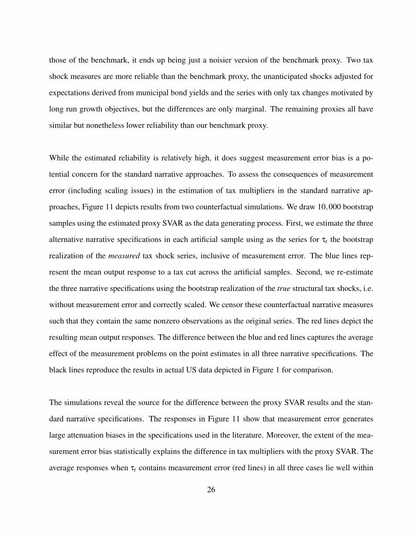
While the estimated reliability is relatively high, it does suggest measurement error bias is a po-

tential concern for the standard narrative approaches. To assess the consequences of measurement

error (including scaling issues) in the estimation of tax multipliers in the standard narrative ap-

proaches, Figure 11 depicts results from two counterfactual simulations. We draw 10,000 bootstrap

samples using the estimated proxy SVAR as the data generating process. First, we estimate the three

alternative narrative specifications in each artificial sample using as the series for τt the bootstrap

realization of the measured tax shock series, inclusive of measurement error. The blue lines rep-

resent the mean output response to a tax cut across the artificial samples. Second, we re-estimate

the three narrative specifications using the bootstrap realization of the true structural tax shocks, i.e.

without measurement error and correctly scaled. We censor these counterfactual narrative measures

such that they contain the same nonzero observations as the original series. The red lines depict the

resulting mean output responses. The difference between the blue and red lines captures the average

effect of the measurement problems on the point estimates in all three narrative specifications. The

black lines reproduce the results in actual US data depicted in Figure 1 for comparison.

The simulations reveal the source for the difference between the proxy SVAR results and the stan-

dard narrative specifications. The responses in Figure 11 show that measurement error generates

large attenuation biases in the specifications used in the literature. Moreover, the extent of the mea-

surement error bias statistically explains the difference in tax multipliers with the proxy SVAR. The

average responses when τt contains measurement error (red lines) in all three cases lie well within

26

the confidence bands of the impulse response estimates. For the Favero and Giavazzi (2012) spec-

ification, the average simulated response aligns almost perfectly with the response in the actual US

data at all horizons. For the other two specifications, which contain a moving average term of τt ,

the simulated output effects are very similar to the actual estimates for horizons up to one year.

At longer horizons, the simulated response is lower than the actual estimates but never leaves the

95% confidence bands. When the true tax shocks are used as the narrative measure (red lines), the

average responses to a tax cut across all specifications are significantly higher and are all close to

the true response in the data generating process in Figure 3. Another result from the simulations is

that, regardless of whether τt contains measurement error and despite the differences in the reduced

form transmission mechanism, the average simulated responses are quantitatively always very sim-

ilar across all three time series specifications. This finding corroborates the simulation evidence of

Charhour, Schmitt-Grohe and Uribe (2012), who use an alternative data generating process based

on the estimated DSGE model of Mertens and Ravn (2011a) to evaluate the ability of the different

specifications to uncover the theoretical response to an unanticipated tax shock. They also find that

the assumed reduced form transmission mechanism is an unlikely source of the difference in esti-

mates in the literature.

In the case of the Favero-Giavazzi model, a straightforward correction for measurement error is

simply to rescale the impulse response such that tax revenues drop by one percentage point of GDP

on impact. This adjustment not only eliminates the scaling problem mentioned earlier, but in case

τt is given by (8) also corrects for the additive error. This is because the Favero-Giavazzi model

includes a single error-ridden regressor that is by assumption uncorrelated with the other regres-

sors. Additive measurement error implies a proportional and identical attenuation bias equal to Λ in

every equation such that impulse responses are correct up to scale. Figure 12 shows that the adjust-

ment almost completely resolves the difference with the proxy SVAR. Based on the estimate for Λ,

around 40% of the difference between the impact coefficients is explained by bias due to additive

27

measurement error, whereas the remainder is due to differences between the impact on projected

tax liabilities versus actual revenues. This decomposition may be different for alternative assump-

tions about the nature of the measurement error. Figure 12 does not report confidence bands for the

adjusted Favero-Giavazzi estimates, which are very wide because the ratio of impact coefficients is

very imprecisely estimated. The same adjustment is not appropriate for the other narrative specifi-

cations because they include multiple error-ridden regressors.

We conclude that a reconciliation with the findings of the existing narrative estimates can be found

in a more careful treatment of measurement problems. The proxy SVAR results imply that, once

measurement error is allowed for, the narrative data is supportive for relatively large tax multipliers

even in the short run.

5 Concluding Remarks and Directions for Future Research

A burgeoning empirical literature on the aggregate effects of changes in tax policy has produced a

range of estimates of the effects on economic activity sufficiently broad that one might question the

value of the findings. In this paper, we analyze the underlying reasons for the disagreement among

the various methodologies. We do this by an application of a structural vector autoregression in

which tax shocks are identified by proxies based on narrative tax shock measures. Our proxy SVAR

estimates large tax multipliers in US data with relatively high precision. A comparison with the

popular Blanchard and Perotti (2002) approach reveals a fundamental conflict in the cyclical adjust-

ment of tax revenues. We argue that the output elasticity of tax revenues is significantly greater than

calculated by international organizations. Differences with earlier narrative studies can be explained

by measurement error, which our proxy SVAR identifies in the data. The evidence in this paper is

supportive for tax multipliers that are at the higher end of the range, such as those of Mountford and

Uhlig (2009) and Romer and Romer (2010), and rejects the lower estimates of for instance Blan-

28

chard and Perotti (2002) and Favero and Giavazzi (2012). Unlike all these studies, however, we also

find large output effects of tax changes in the short run.

There are several directions for future research. Our analysis raises concerns with the cyclical ad-

justment procedures of government and international institutions and calls for alternative, structural,

approaches to the estimation of the output elasticity of tax revenues. This is important since this

elasticity is a vital ingredient of policy evaluations, budget forecasting, and other empirical work,

e.g. on fiscal consolidations by Alesina and Ardagna (2010). In focusing attention on cyclical ad-

justment and measurement error, we followed the common practice of studying the effects of shocks

to total revenues in linear models. Other aspects of the empirical study of tax policy shocks, such

as the dependence on the type of the tax instrument being adjusted or the possible time-varying na-

ture of tax multipliers can be incorporated. Given that narrative measures of policy shocks become

increasingly available, our analysis can be repeated in the future for other countries as well as for

other types of shocks. Finally, our analysis is also informative about features that can improve the

explanatory and predictive power of theoretical models of fiscal policy. These features are likely to

include large tax multipliers and high output elasticities of tax revenues.

References

Alesina, Alberto and Silvia Ardagna, 2010, “Large Changes in Fiscal Policy: Taxes versus Spend-ing”, NBER Chapters, in: Tax Policy and the Economy Vol. 24, pp. 35–68.

Auerbach, Alan J., and Yuriy Gorodnichenko, 2012, “Measuring the Output Responses to FiscalPolicy,” forthcoming, American Economic Journal: Economic Policy.

Barro, Robert J. and Charles J. Redlick, 2011, “ The Macroeconomic Effects of GovernmentPurchases and Taxes”, Quarterly Journal of Economics 126(1),pp. 51–102.

Bernanke, Ben S., Jean Boivin and Piotr Eliasz, 2005, “Measuring the Effects of Monetary Pol-icy: A Factor-Augmented Vector Autoregressive (FAVAR) Approach”, Quarterly Journal of Eco-nomics, 120(1), pp. 387–422.

29

Blanchard, Olivier and Roberto Perotti, 2002, “An Empirical Characterization of the DynamicEffects of Changes in Government Spending and Taxes on Output”, Quarterly Journal of Eco-nomics 117(4), pp. 1329–1368.

Bornhorst, Fabian, Gabriela Dobrescu, Annalisa Fedelino, Jan Gottschalk, and TaisukeNakata, 2011, “When and How to Adjust Beyond the Business Cycle? A Guide to StructuralFiscal Balances”, Technical Notes and Manual, Fiscal Affairs, International Monetary Fund.

Bruckner, Markus, 2011, “An Instrumental Variables Approach to Estimating Tax Revenue Elas-ticities: Evidence from Sub-Saharan Africa”, forthcoming, Journal of Development Economics.

Congressional Budget Office, 2010,“The Effects of Automatic Stabilizers on the Federal Budget”,CBO Report.

Caballe, Jordi and Judith Panades, 2011. “Tax Evasion, Technology Shocks, and the Cyclicalityof Government Revenues,” UFAE and IAE Working Papers 870.11, Universitat Autonoma deBarcelona

Canova, Fabio and Evi Pappa, 2007, “Price Differentials in Monetary Unions: The Role of FiscalShocks”, Economic Journal 117(4), pp. 713–737.

Caldara, Dario and Christophe Kamps, 2008, “What Are the Effects of Fiscal Shocks: A VAR-Based Comparative Analyis.”, ECB Working Paper No 877.

Caldara, Dario and Christophe Kamps, 2012, “The Analytics of SVARs: A Unified Frameworkto Measure Fiscal Multipliers”, manuscript, Board of Governors.

Charhour, Ryan, Stephanie Schmitt-Grohe and Martin Uribe, 2012, “A Model-Based Evalua-tion of the Debate on the Size of the Tax Multiplier”, forthcoming Americal Economic Journal:Economic Policy.

Cloyne, James, 2012, “What Are the Effects of Tax Changes in the United Kingdom? New Evi-dence from a Narrative Evaluation”, manuscript, Bank of England

Cohen, Darrel and Glenn Follette, 2000, “The Automatic Fiscal Stabilizers: Quietly Doing TheirThing”, Federal Reserve Bank of New York Economic Policy Review April 2000, pp. 35—67.

Fatas, Antonio and Ilian Mihov, 2001, “The Effects of Fiscal Policy on Consumption and Em-ployment: Theory and Evidence”, CEPR Discussion Papers No. 2760.

Favero, Carlo and Francesco Giavazzi, 2012,“Measuring Tax Multipliers. The Narrative Methodin Fiscal VARs”. American Economic Journal: Economic Policy, forthcoming.

Favero, Carlo and Francesco Giavazzi and Jacopo Perego, 2011, “Country Heterogeneity andthe International Evidence on the Effects of Fiscal Policy”, IMF Economic Review November,pp. 652–82.

30

Fisher, Jonas D.M. and Ryan Peters, 2010, “Using Stock Returns to Identify Government Spend-ing Shocks”, Economic Journal 120(544), pp. 414–436.

Follette, Glenn and Byron Lutz, 2010, “Fiscal Policy in the United States: Automatic Stabilizers,Discretionary Fiscal Policy Actions, and the Economy”, manuscript, Board of Governors

Francis, Neville and Valerie A. Ramey, 2009, “Measures of per Capita Hours and Their Impli-cations for the Technology-Hours Debate”, Journal of Money, Credit and Banking 41(6), 1071-1097.

Girouard, Nathalie and Christophe Andre, 2005, “Measuring Cyclically Adjusted Budget Bal-ances for OECD Countries”, OECD Economics Department Working Papers No. 434, OECDPublishing.

Giorno, Claude, Pete Richardson, Deborah Roseveare and Paul van den Noord, 1995, “Esti-mating Potential Output, Output Gaps and Structural Budget Balances”, OECD Economics De-partment Working Papers no.152.

Goncalves, Silvia and Lutz Kilian, 2004, “Bootstrapping Autoregressions with Conditional Het-eroskedasticity of Unknown Form”, Journal of Econometrics 123(1), pp. 89–120.

Hausman, Jerry A. and William E. Taylor, 1983, “Identification in Linear Simultaneous EquationModels with Covariance Restrictions: An Instrumental Variables Interpretation”, Econometrica51(5), pp.1527-1549.

Hsiao, Cheng, 1979, “Measurement Error in a Dynamic Simultaneous Equations Model with Sta-tionary Disturbances”, Econometrica 47(2), pp. 475–494.

Ilzetzki, Ethan, 2011, “Fiscal Policy and Debt Dynamics in Developing Countries”, World BankPolicy Research Working Paper Series No. 5666.

Kueng, Lorenz, 2011, “Identifying the Household Consumption Response to Tax Expectationsusing Bond Prices”, manuscript, University of California, Berkeley.

Leeper, Eric M., Todd B. Walker and Shu-Chun Susan Yang, 2011, “Foresight and InformationFlows”, manuscript, Indiana University Bloomington.

Maravall, Agustin and Dennis J. Aigner, 1977, “Identification of the Dynamic Shock-ErrorModel: The Case of Dynamic Regression”, in: Latent Variables in Socio-Economic Models,ed. by Aigner and A. Goldberger, Amsterdam, North Holland.

Mertens, Karel and Morten O. Ravn, 2011a, “Understanding the Aggregate Effects of Anticipatedand Unanticipated Tax Policy Shocks”, Review of Economic Dynamics, 14(1), pp. 27–54.

Mertens, Karel and Morten O. Ravn, 2011b, “Technology - Hours Redux: Tax Changes and theMeasurement of Technology Shocks.”, NBER International Seminar of Macroeconomics 2010,pp. 41–76.

31

Mertens, Karel and Morten O. Ravn, 2012a, “Empirical Evidence on the Aggregate Effects ofAnticipated and Unanticipated U.S. Tax Policy Shocks”, American Economic Journal: EconomicPolicy, forthcoming.

Mertens, Karel and Morten O. Ravn, 2012b, “The Dynamic Effects of Personal and CorporateIncome Tax Changes in the United States”, manuscript, Cornell University and University CollegeLondon.

Mountford, Andrew, and Harald Uhlig, 2009, “What Are the Effects of Fiscal Policy Shocks?”Journal of Applied Econometrics 24(6), pp. 960–992.

Perotti, Roberto, 2005, “Estimating the Effects of Fiscal Policy in OECD Countries”, CEPR Dis-cussion Paper No. 4842.

Perotti, Roberto, 2011, “The Effects of Tax Shocks on Output: Not So Large, But Not SmallEither”, NBER Working Paper No. 16786.

Ramey, Valerie A., 2011, “Identifying Government Spending Shocks: It’s All in the Timing”,Quarterly Journal of Economics 126(1), pp. 10-50.

Romer, Christina D., and David H. Romer, 2009, “A Narrative Analysis of Postwar Tax Changes”manuscript, University of California, Berkeley.

Romer, Christina D., and David H. Romer, 2010, “The Macroeconomic Effects of Tax Changes:Estimates Based on a New Measure of Fiscal Shocks” , American Economic Review 100(3), pp.763–801.

Sancak, Cemile, Ricardo Velloso, and Jing Xing, 2010, “Tax Revenue Response to the BusinessCycle”, IMF Working Paper No. 10/71.

Saez, Emmanuel, Joel B. Slemrod and Seth H. Giertz, 2012,“ The Elasticity of Taxable Incomewith Respect to Marginal Tax Rates: A Critical Review” , Journal of Economic Literature 50(1),pp. 3-50.

Stock, James H. and Mark W. Watson, 2008, “ What’s New in Econometrics - Time Series”,NBER Summer Institute, Lecture 7.

Stock, James H. and Mark W. Watson, 2012, “Disentangling the Channels of the 2007-2009Recession”, Brookings Panel on Economic Activity, Conference Paper March 22-23.

van den Noord, Paul, 2000, “The Size and Role of Automatic Fiscal Stabilizers in the 1990s andBeyond”, OECD Economics Department Working Papers, No. 230, OECD

32

(A) Blanchard and Perotti (2002)

0 2 4 6 8 10 12 14 16 18 20−2

−1

0

1

2

3

4

5

Output

quarters

pe

rce

nt

(B) Romer and Romer (2010)

0 2 4 6 8 10 12 14 16 18 20−2

−1

0

1

2

3

4

5

Output

quarters

pe

rce

nt

(C) Favero and Giavazzi (2012)

0 2 4 6 8 10 12 14 16 18 20−2

−1

0

1

2

3

4

5

Output

quarters

pe

rce

nt

(D) Mertens and Ravn (2012a)

0 2 4 6 8 10 12 14 16 18 20−2

−1

0

1

2

3

4

5

Output

quarters

pe

rce

nt

Figure 1 Replication of Existing Estimates of the Output Response to Tax Cuts. Broken lines in(A), (C) and (D) are 95% bootstrapped percentiles. Broken lines in (B) are ± 2 asymptotic standarderror bands.

1950 1960 1970 1980 1990 20000

5

10

15

20

25

pe

rce

nt

1950 1960 1970 1980 1990 2000−1.5

−1

−0.5

0

0.5

1

Revenues/GDP (Left axis)

Narrative Shocks (Right axis)

Figure 2 The Average Tax Rate and the Narrative Measure of Unanticipated Tax Shocks.

−1.5 −1 −0.5 0 0.5 1−4

−3

−2

−1

0

1

2

3

εT t

m t

Figure 3 Identified Tax Shocks and the Proxy Measure

0 2 4 6 8 10 12 14 16 18 20−2

−1

0

1

2

3

4

5

Output

quarters

pe

rce

nt

0 2 4 6 8 10 12 14 16 18 20−10

−8

−6

−4

−2

0

2

4

6

8

10Tax Revenues

quarters

pe

rce

nt

0 2 4 6 8 10 12 14 16 18 20−10

−8

−6

−4

−2

0

2

4

6

8

10Government Spending

quarters

pe

rce

nt

Figure 4 Proxy SVAR: Response to a Tax Cut of 1% of GDP. Broken lines are 95% bootstrappedpercentiles.

(A) Alternative Narrative Measures

0 2 4 6 8 10 12 14 16 18 20−1

0

1

2

3

4

5

6

7Output

quarters

pe

rce

nt

Benchmark

Long Run Only

Retroactive

Scaled by Yt−4

(B) Trend Assumptions

0 2 4 6 8 10 12 14 16 18 20−1

0

1

2

3

4

5

6

7Output

quarters

pe

rce

nt

Deterministic Trend

Stochastic Trend

(C) Including Fiscal Foresight Variables

0 2 4 6 8 10 12 14 16 18 20−1

0

1

2

3

4

5

6

7Output

quarters

pe

rce

nt

Benchmark

Implicit Tax Rate

Defense returns

Defense news

(D) Anticipation Adjusted Proxy

0 2 4 6 8 10 12 14 16 18 20−1

0

1

2

3

4

5

Output

quarters

pe

rce

nt

Benchmark

Anticipation Adjusted

Using all Exogenous Romer and Romer (2009) shocks:

(E) Unadjusted Proxy

0 2 4 6 8 10 12 14 16 18 20−1

0

1

2

3

4

5

Output

quarters

pe

rce

nt

Benchmark

All Romer Shocks

(F) Anticipation Adjusted Proxy

0 2 4 6 8 10 12 14 16 18 20−1

0

1

2

3

4

5

Output

quarters

pe

rce

nt

Benchmark

Anticipation Adjusted

Figure 5 Robustness of Proxy SVAR. Broken lines are 95% bootstrapped percentiles.

0 2 4 6 8 10 12 14 16 18 20−1

0

1

2

3

4

5

Output

quarters

pe

rce

nt

Proxy SVAR

Blanchard Perotti SVAR with θY=3.13

Figure 6 Tax Multiplier: Reconciling the SVARestimates. Broken lines are 95% bootstrappedpercentiles.

0 2 4 6 8 10 12 14 16 18 20−1

−0.5

0

0.5

1

1.5

2

2.5

3Output

quarters

pe

rce

nt

Proxy SVAR

Blanchard Perotti SVAR

Figure 7 Response to a Spending Shock of 1%of GDP. Broken lines are 95% bootstrapped per-centiles.

(A) Blanchard-Perotti SVAR

0 2 4 6 8 10 12 14 16 18 20−1

0

1

2

3

4

5

Output

quarters

pe

rce

nt

1950−1979

1980−2006

(B) Proxy SVAR

0 2 4 6 8 10 12 14 16 18 20−1

0

1

2

3

4

5

Output

quarters

pe

rce

nt

1950−1979

1980−2006

Figure 8 Subsample Stability. Broken lines are 95% bootstrapped intervals of the benchmarkspecification.

1950 1960 1970 1980 1990 2000−15

−10

−5

0

5

10

15

20

25Tax Revenues

pe

rce

nt

de

v. fr

om

tre

nd

Cyclical Component: Blanchard−Perotti SVAR

Cyclical Component: Proxy SVAR

Actual

Figure 9 Actual and Cyclical Components of Tax Revenues Percent deviations from trend. Greyareas are NBER dated recessions.

2007 2008 2009 2010 2011−30

−25

−20

−15

−10

−5

0

5Tax Revenues

pe

rce

nt

Cyclical: Blanchard−Perotti SVAR

Cyclical: Proxy SVAR

Actual

2007 2008 2009 2010 2011−9

−8

−7

−6

−5

−4

−3

−2

−1

0

1

2Output

pe

rce

nt

Figure 10 The Great Recession: Cyclical versus Actual Drop in Tax Revenues (Left) and ActualOutput (Right). Percent deviations from 2007:Q4 levels. Grey area is the NBER dated recession.

(A) Romer and Romer (2010)

0 2 4 6 8 10 12 14 16 18 20−2

−1

0

1

2

3

4

5

Output

quarters

pe

rce

nt

(B) Favero and Giavazzi (2012)

0 2 4 6 8 10 12 14 16 18 20−2

−1

0

1

2

3

4

5

Output

quarters

pe

rce

nt

(C) Mertens and Ravn (2012a)

0 2 4 6 8 10 12 14 16 18 20−2

−1

0

1

2

3

4

5

Output

quarters

pe

rce

nt

US Data

Simulation with Measurement Error

Simulation without Measurement Error

Figure 11 The Role of Measurement Error in Standard Narrative Approaches.

0 2 4 6 8 10 12 14 16 18 20−1

0

1

2

3

4

5

Output

quarters

pe

rce

nt

Proxy SVAR

Favero Giavazzi Measurement Adjusted

Figure 12 Proxy SVAR and Favero and Giavazzi (2012) Adjusted for Measurement Error.Broken lines are 95% bootstrapped percentiles.

Table 1 Parameter Estimates

Proxy SVAR Blanchard-Perotti SVAR

Equation Benchmark θY = 2.08 θY = 3.13

Tax Revenue θG −0.20 −0.06 −0.13[−0.35,−0.07] [−0.12,−0.03] [−0.19,−0.09]

θY 3.13 2.08 3.13[2.73,3.55] – –

σT ×100 2.54 2.24 2.56[2.23,2.62] [2.04,2.19] [2.34,2.51]

Spending γT 0.06 0 0[−0.06,0.17] – –

γY 0 0 0– – –

σG ×100 2.35 2.36 2.36[2.12,2.30] [2.13,2.31] [2.13,2.31]

Output ζT −0.36 −0.08 −0.36[−0.57,−0.24] [−0.11,−0.06] [−0.43,−0.31]

ζG 0.10 0.07 0.10[0.06,0.13] [0.06,0.09] [0.07,0.12]

σY ×100 1.54 0.97 1.54[1.21,1.93] [0.89,0.98] [1.37,1.64]

Values in parenthesis are 95% percentiles computed using 10,000 bootstrap replications.

Table 2 Parameter Estimates using Different Proxy Measures for Tax Shocks

Proxy Used Output Elasticity Reliabilityof Tax Revenues, θy

Benchmark (Figure 3) 3.13 0.57[2.73,3.55] [0.50,0.61]

Long Run Shocks Only (Figure 4, A) 2.94 0.60[2.56, 3.33] [0.56, 0.63]

Including Retroactive Provisions (Figure 4, A) 3.30 0.48[2.78 3.87] [0.35, 0.54]

Scaled by Yt−4 (Figure 4, A) 3.14 0.57[2.73 3.57] [0.45 0.61]

Benchmark, Anticipation Adjusted (Figure 4, D) 2.88 0.59[2.53, 3.25] [0.53, 0.63]

All Romer Tax Shocks (Figure 4, E) 1.84 0.34[1.47, 2.29] [0.25,0.42]

All Romer Tax Shocks, Anticipation Adjusted (Figure 4, F) 2.70 0.22[2.07, 3.53] [0.13, 0.30]

Values in parenthesis are 95% percentiles computed using 10,000 bootstrap replications.