THE KATZ-KLEMM-VAFA CONJECTURE FOR K3SURFACES

R. PANDHARIPANDE AND R.P. THOMAS

Abstract. We prove the KKV conjecture expressing Gromov-Witten invariants of K3 surfaces in terms of modular forms. Ourresults apply in every genus and for every curve class. The proofuses the Gromov-Witten/Pairs correspondence for K3-fibered hy-persurfaces of dimension 3 to reduce the KKV conjecture to state-ments about stable pairs on (thickenings of) K3 surfaces. Usingdegeneration arguments and new multiple cover results for stablepairs, we reduce the KKV conjecture further to the known primi-tive cases.

Our results yield a new proof of the full Yau-Zaslow formula,establish new Gromov-Witten multiple cover formulas, and expressthe fiberwise Gromov-Witten partition functions of K3-fibered 3-folds in terms of explicit modular forms.

Contents

0. Introduction 21. Noether-Lefschetz theory 14

2. Anticanonical K3 surfaces in ˜P2 × P1 213. Theorem 2 254. K3× C: Localization 305. K3× C: Vanishing 426. Relative theory and the logarithm 527. Multiple covers 848. P/NL correspondence 909. Katz-Klemm-Vafa conjecture 11110. Quartic K3 surfaces 112Appendix A. Invariants 113Appendix B. Degenerations 115Appendix C. Cones and virtual classes 117References 122

Date: April 2016.1

0. Introduction

0.1. Reduced Gromov-Witten theory. Let S be a nonsingular pro-

jective K3 surface, and let

β ∈ Pic(S) = H2(S,Z) ∩H1,1(S,C)

be a nonzero effective curve class. The moduli space M g(S, β) of genus

g stable maps (with no marked points) has expected dimension

dimvirC Mg(S, β) =

∫

β

c1(S) + (dimC(S)− 3)(1− g) = g − 1 .

However, as the obstruction theory admits a 1-dimensional trivial quo-

tient, the virtual class [M g(S, β)]vir vanishes. The standard Gromov-

Witten theory is trivial.

Curve counting on K3 surfaces is captured instead by the reduced

Gromov-Witten theory constructed first via the twistor family in [8].

An algebraic construction following [2, 3] is given in [35]. The reduced

class

[M g(S, β)]red ∈ Ag(M g(S, β),Q)

has dimension g. Let λg be the top Chern class of the rank g Hodge

bundle1

Eg →M g(S, β)

with fiber H0(C, ωC) over the moduli point

[f : C → S] ∈M g(S, β) .

The reduced Gromov-Witten integrals of S,

(0.1) Rg,β(S) =

∫

[Mg(S,β)]red(−1)gλg ∈ Q ,

are well-defined. Under deformations of S for which β remains a (1, 1)-

class, the integrals (0.1) are invariant.

Let ǫ : X → (B, b) be a fibration of K3 surfaces over a base B with

special fiber

Xb∼= S over b ∈ B .

1The Hodge bundle is pulled-back fromMg if g ≥ 2. See [13, 18] for a discussionof Hodge classes in Gromov-Witten theory.

2

Let U ⊂ B be an open set containing b ∈ B over which the local

system of second cohomology R2ǫ∗(Z) is trivial. The class β ∈ Pic(S)

determines a local Noether-Lefschetz locus

NL(β) ⊂ U

defined as the subscheme where β remains a (1, 1)-class.2

Let (∆, 0) be a nonsingular quasi-projective curve with special point

0 ∈ ∆. The integral Rg,β(S) computes the local contribution of S to

the standard Gromov-Witten theory of every K3-fibered 3-fold

(0.2) ǫ : T → (∆, 0)

with special fiber S and local Noether-Lefschetz locus NL(β) ⊂ ∆ equal

to the reduced point 0 ∈ ∆, see [35].

0.2. Curve classes. The second cohomology of S is a rank 22 lattice

with intersection form

(0.3) H2(S,Z)∼= U ⊕ U ⊕ U ⊕ E8(−1)⊕E8(−1) ,

where

U =

(0 11 0

)

and

E8(−1) =

−2 0 1 0 0 0 0 00 −2 0 1 0 0 0 01 0 −2 1 0 0 0 00 1 1 −2 1 0 0 00 0 0 1 −2 1 0 00 0 0 0 1 −2 1 00 0 0 0 0 1 −2 10 0 0 0 0 0 1 −2

is the (negative) Cartan matrix. The intersection form (0.3) is even.

The divisibility m(β) is the maximal positive integer dividing the

lattice element β ∈ H2(S,Z). If the divisibility is 1, β is primitive.

Elements with equal divisibility and norm square are equivalent up to

2While NL(β) is locally defined on U by a single equation, the locus may bedegenerate (equal to all of U).

3

orthogonal transformation ofH2(S,Z), see [46]. By straightforward de-

formation arguments using the Torelli theorem forK3 surfaces, Rg,β(S)

depends, for effective classes, only on the divisibilitym(β) and the norm

square

〈β, β〉 =∫

S

β2 .

We will omit the argument S in the notation,

Rg,β = Rg,β(S) .

0.3. BPS counts. The KKV conjecture concerns BPS counts associ-

ated to the Hodge integrals (0.1). Throughout this paper we let

α ∈ Pic(S)

denote a nonzero class which is both effective and primitive. The

Gromov-Witten potential Fα(λ, v) for classes proportional to α is

(0.4) Fα =∑

g≥0

∑

m>0

Rg,mα λ2g−2vmα.

The BPS counts rg,mα are uniquely defined by the following equation:

(0.5) Fα =∑

g≥0

∑

m>0

rg,mα λ2g−2

∑

d>0

1

d

(sin(dλ/2)

λ/2

)2g−2

vdmα.

Equation 0.5 defines BPS counts for both primitive and divisible classes.

The string theoretic calculations of Katz, Klemm and Vafa [23] via

heterotic duality yield two conjectures.

Conjecture 1. The BPS count rg,β depends upon β only through the

norm square 〈β, β〉.

Conjecture 1 is rather surprising from the point of view of Gromov-

Witten theory. From the definition, the invariants Rg,β and rg,β depend

upon both the divisibility m of β and the norm square 〈β, β〉. Assuming

the validity of Conjecture 1, let rg,h denote the BPS count associated

to a class β of arithmetic genus h,

〈β, β〉 = 2h− 2 .4

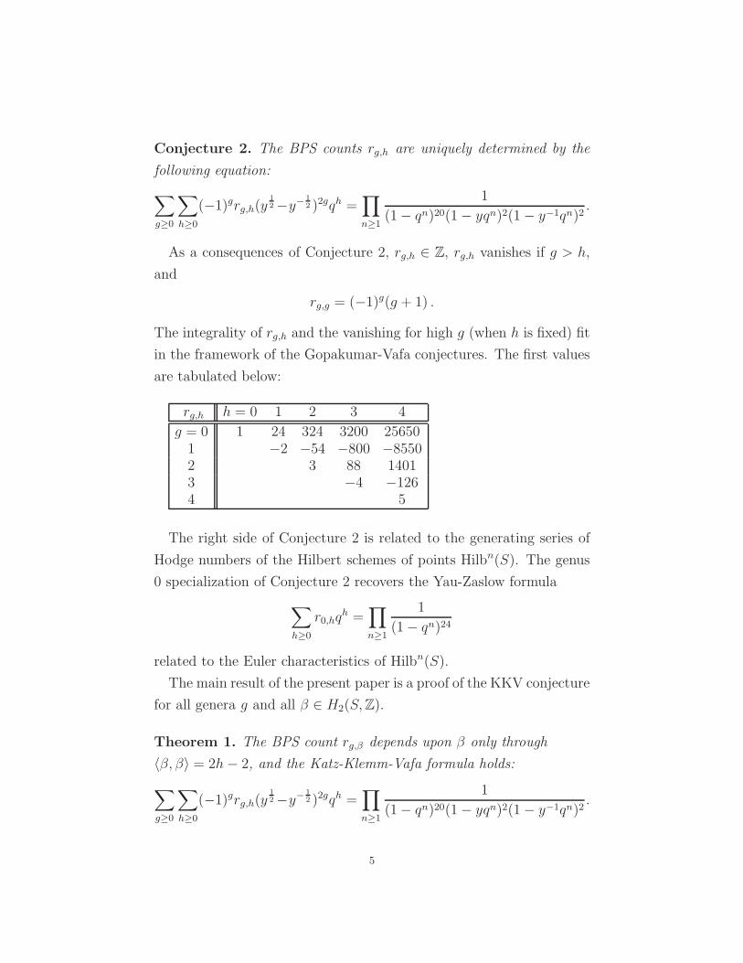
Conjecture 2. The BPS counts rg,h are uniquely determined by the

following equation:

∑

g≥0

∑

h≥0

(−1)grg,h(y12 −y− 1

2 )2gqh =∏

n≥1

1

(1− qn)20(1− yqn)2(1− y−1qn)2.

As a consequences of Conjecture 2, rg,h ∈ Z, rg,h vanishes if g > h,

and

rg,g = (−1)g(g + 1) .

The integrality of rg,h and the vanishing for high g (when h is fixed) fit

in the framework of the Gopakumar-Vafa conjectures. The first values

are tabulated below:

rg,h h = 0 1 2 3 4

g = 0 1 24 324 3200 256501 −2 −54 −800 −85502 3 88 14013 −4 −1264 5

The right side of Conjecture 2 is related to the generating series of

Hodge numbers of the Hilbert schemes of points Hilbn(S). The genus

0 specialization of Conjecture 2 recovers the Yau-Zaslow formula

∑

h≥0

r0,hqh =

∏

n≥1

1

(1− qn)24

related to the Euler characteristics of Hilbn(S).

The main result of the present paper is a proof of the KKV conjecture

for all genera g and all β ∈ H2(S,Z).

Theorem 1. The BPS count rg,β depends upon β only through

〈β, β〉 = 2h− 2, and the Katz-Klemm-Vafa formula holds:

∑

g≥0

∑

h≥0

(−1)grg,h(y12 −y− 1

2 )2gqh =∏

n≥1

1

(1− qn)20(1− yqn)2(1− y−1qn)2.

5

0.4. Past work. The enumerative geometry of curves on K3 surfaces

has been studied since the 1995 paper of Yau and Zaslow [47]. A math-

ematical approach to the genus 0 Yau-Zaslow formula can be found in

[4, 11, 14]. The Yau-Zaslow formula was proven for primitive classes

β by Bryan and Leung [8]. The divisibility 2 case was settled by Lee

and Leung in [31]. A complete proof of the Yau-Zaslow formula for all

divisibilities was given in [27]. Our approach to Theorem 1 provides

a completely new proof of the Yau-Zaslow formula for all divisibili-

ties (which avoids the mirror calculation of the STU model and the

Harvey-Moore identity used in [27]).

Conjecture 2 for primitive classes β is connected to Euler character-

istics of the moduli spaces of stable pairs on K3 surfaces by the GW/P

correspondence of [39, 40]. A proof of Conjecture 2 for primitive classes

is given in [36] relying upon the Euler characteristic calculations of

Kawai and Yoshioka [24]. For cases where g > 0 and β is not primitive,

Theorem 1 is a new result.

The cases understood before are very special. If the genus is 0, the

calculation can be moved via Noether-Lefschetz theory to the genus 0

Gromov-Witten theory of toric varieties using the hyperplane principle

for K3-fibrations [27]. If the class β is irreducible, the moduli space of

stable pairs is nonsingular [24], and the calculation can be moved to

stable pairs [36]. The difficulty for positive genus imprimitive curves –

which are essentially all curves – lies in the complexity of the moduli

spaces. There is no effective hyperplane principle in higher genus, and

the moduli spaces of stable maps and stable pairs are both highly

singular.

Y. Toda has undertaken a parallel study of the Euler characteristic

(following Joyce) of the moduli spaces of stable pairs on K3 surfaces

[45]. His results – together with further multiple cover conjectures

which are still open – are connected to an Euler characteristic version

of the KKV formula. Our methods and results essentially concern the

virtual class and thus do not imply (nor are implied by) Toda’s paper

6

[45]. In fact, the motivation of [45] was the original KKV conjecture

proven here.

0.5. GW/P correspondence. The Katz-Klemm-Vafa formula con-

cerns integrals over the moduli space of stable maps. Our strategy is

to transform the calculation to the theory of stable pairs. Let P2 × P1

be the blow up of P2×P1 in a point. Consider a nonsingular anticanon-

ical Calabi-Yau 3-fold hypersurface,

X ⊂ P2 × P1 × P1 .

The projection onto the last factor,

(0.6) π3 : X → P1 ,

determines a 1-parameter family of anticanonicalK3 surfaces in P2 × P1.

The interplay between the Gromov-Witten, stable pairs, and Noether-

Lefschetz theories for the family π3 will be used to transform Theorem

1 to nontrivial claims about of the moduli of sheaves on K3-fibrations.

The KKV formula (conjecturally) evaluates the integrals Rg,β occur-

ring in the reduced Gromov-Witten theory of a K3 surface S. If we

view S as a fiber of π3, then

β ∈ Pic(S) ⊂ H2(S,Z) ∼= H2(S,Z)

determines a fiber class in H2(X,Z) by push-forward. We consider

both the Gromov-Witten and stable pairs invariants of X in π3-fiber

curve classes. The GW/NL correspondence of [35] precisely relates the

Gromov-Witten theory of X in fiber classes with the Noether-Lefschetz

numbers of the family and the integrals Rg,β. We prove a P/NL corre-

spondence which establishes a parallel relationship between the stable

pairs theory of X in fiber classes with the same Noether-Lefschetz num-

bers and the invariants Rn,β defined as follows.

0.6. Stable pairs and K3 surfaces. Let S be a nonsingular projec-

tive K3 surface with a nonzero effective curve class β ∈ Pic(S). We de-

fine here the stable pairs analogue Rn,β of the reduced Gromov-Witten

invariants Rg,β of S.7

For Gromov-Witten invariants, we defined Rg,β directly (0.1) in terms

of the moduli of stable maps to S and observed the result calculated the

contributions of the special fiber S to the Gromov-Witten theories of all

families (0.2) appropriately transverse to the local Noether-Lefschetz

locus corresponding to β. The geometry of stable pairs is more subtle.

While the support of a stable pair may probe thickenings of the special

fiber S ⊂ T of (0.2), the image of a stable map does not. As a result,

we will define Rn,β via the geometry of appropriately transverse fam-

ilies of K3 surfaces. Later in Section 6.11, we will see how to define

Rn,β via the intrinsic geometry of S.

Let α ∈ Pic(S) be a nonzero class which is both effective and prim-

itive. Let T be a nonsingular 3-dimensional quasi-projective variety,

ǫ : T → (∆, 0) ,

fibered in K3 surfaces over a pointed curve (∆, 0) satisfying:

(i) ∆ is a nonsingular quasi-projective curve,

(ii) ǫ is smooth, projective, and ǫ−1(0)∼= S,

(iii) the local Noether-Lefschetz locus NL(α) ⊂ ∆ corresponding to

the class α ∈ Pic(S) is the reduced point 0 ∈ ∆.

The class α ∈ Pic(S) is m-rigid with respect to the family ǫ if the

following further condition is satisfied:

(⋆) for every effective decomposition3

mα =

l∑

i=1

γi ∈ Pic(S) ,

the local Noether-Lefschetz locus NL(γi) ⊂ ∆ corresponding to

each class γi ∈ Pic(S) is the reduced point 0 ∈ ∆.

Let Eff(mα) ⊂ Pic(S) denote the subset of effective summands of mα.

Condition (⋆) implies (iii).

Assume α is m-rigid with respect to the family ǫ. By property (⋆),

there is a compact, open, and closed component

P ⋆n(T, γ) ⊂ Pn(T, γ)

3An effective decomposition requires all parts γi to be effective divisors.8

parameterizing stable pairs4 supported set-theoretically over the point

0 ∈ ∆ for every effective summand γ ∈ Eff(mα).

Definition. Let α ∈ Pic(S) be a nonzero class which is both effective

and primitive. Given a family ǫ : T → (∆, 0) satisfying conditions (i),

(ii), and (⋆) for mα, let

(0.7)∑

n∈Z

Rn,mα(S) qn =

Coeffvmα

log

1 +

∑

n∈Z

∑

γ∈Eff(mα)

qnvγ∫

[P ⋆n(T,γ)]

vir

1

.

In Section 6.12, we will prove Rn,mα depends only upon n, m and

〈α, α〉, and not upon S nor the family ǫ. The dependence result is

nontrivial and requires new techniques to establish. The existence5 of

m-rigid families ǫ for suitable S and α (primitive with fixed 〈α, α〉)then defines Rn,mα for all m.

The appearance of the logarithm in (0.7) has a simple explanation.

The Gromov-Witten invariants Rg,mα are defined via moduli spaces

of stable maps with connected domains. Stable pairs invariants count

sheaves with possibly disconnected support curves. The logarithm ac-

counts for the difference.

The stable pairs potential Fα(q, v) for classes proportional to the

primitive class α is

(0.8) Fα =∑

n∈Z

∑

m>0

Rn,mα qnvmα .

By the properties of Rn,mα, the potential Fα depends only upon the

norm square 〈α, α〉.Via the correspondences with Noether-Lefschetz theory, we prove

that the GW/P correspondence [38, 39] for suitable 3-folds fibered in

4For any class γ ∈ Pic(S), we denote the push-forward to H2(T,Z) also by γ.Let Pn(T, γ) be the moduli space of stable pairs of Euler characteristic n and classγ ∈ H2(T,Z).

5Constructions are given in Section 6.2.9

K3 surfaces implies the following basic result for the potentials (0.4)

and (0.8).

Theorem 2. After the variable change −q = eiλ, the potentials are

equal:

Fα(λ, v) = Fα(q, v)

In order to show the variable change of Theorem 2 is well defined, a

rationality result is required. In Section 7, we prove for all m > 0,[Fα

]vmα

=∑

n∈Z

Rn,mα qn

is the Laurent expansion of a rational function in q.

0.7. Multiple covers. While Theorem 2 transforms Theorem 1 to a

statement about stable pairs, the evaluation must still be carried out.

The logarithm in definition (0.7) plays no role for the vα coefficient,[Fα

]vα

=∑

n∈Z

qn∫

[P ⋆n(T,α)]

vir

1 .

If α is irreducible (which can be assumed by deformation invariance),

P ⋆n(T, α) is a nonsingular variety of dimension 〈α, α〉 + n + 1. If T is

taken to be Calabi-Yau, the obstruction theory on P ⋆n(T, α) is self-dual

and∑

n∈Z

qn∫

[Pn(T,α)]vir1 =

∑

n∈Z

qn(−1)〈α,α〉+n+1 χtop (P⋆n(T, α)) .

The Euler characteristic calculations of Kawai and Yoshioka [24] then

imply the stable pairs KKV prediction for primitive α ∈ Pic(S). A

detailed discussion can be found in Appendix C of [40].

In order to prove the KKV conjecture for[Fα

]vmα

for all m > 1, we

find new multiple cover formulas for stable pairs on K3 surfaces. In

fact, the multiple cover structure implicit in the KKV formula is much

more natural on the stable pairs side.

By degeneration arguments and deformation to the normal cone,

we reduce the stable pairs multiple cover formula to a calculation on

the trivial K3-fibration S×C, where C∗-localization applies. A crucial10

point here is a vanishing result: for each k only the simplest k-fold mul-

tiple covers contribute – those stable pairs which are a trivial k-times

thickening in the C-direction of a stable pair on S. The moduli space

of such trivial thickenings is isomorphic to the moduli space of stable

pairs supported on S. This simple geometric relationship provides the

key to the stable pairs multiple cover formula.

0.8. Guide to the proof. The main steps in our proof of the Katz-

Klemm-Vafa formula are summarized as follows:

(i) We express the Gromov-Witten invariants of the anticanonical

hypersurface,

X ⊂ P2 × P1 × P1 ,

in terms of the Noether-Lefschetz numbers of π3 and the re-

duced invariants Rg,β via the GW/NL correspondence.

(ii) We express the stable pairs invariants of X in terms of the

Noether-Lefschetz numbers of π3 and the stable pairs invari-

ants Rn,β via the P/NL correspondence.

(iii) The GW/P conjecture, proved for the complete intersection X

in [38], relates the Gromov-Witten and stable pairs invariants

of the 3-fold X.

(iv) By inverting the relations (i) and (ii) and using the correspon-

dence (iii), we establish the equivalence between the sets of

numbers Rg,β and Rn,β stated in Theorem 2.

(v) The invariant Rn,β(S) is defined via an appropriately transverse

family

ǫ : T → (∆, 0) , ǫ−1(0)∼= S .

Degenerating the total space T to the normal cone of S ⊂ T , we

reduce Rn,β(S) to a calculation of stable pairs integrals over a

rubber target. After further geometric arguments, the calcula-

tion is expressed in terms of the reduced stable pairs invariants

of the trivial K3-fibration S × P1. A careful analysis of several

different obstruction theories is required here.11

(vi) By C∗-localization on S×P1, we reduce further to a calculation

on the moduli space of C∗-fixed stable pairs on S × C.

(vii) We prove a vanishing result: for each k only the simplest k-fold

multiple covers contribute. We only need calculate the contri-

butions of stable pairs which are a trivial k-times thickening (in

the C-direction) of a stable pair scheme-theoretically supported

on S.

(viii) The resulting moduli spaces are isomorphic to Pn(S, β), the

moduli space of stable pairs on S.

(ix) The resulting integral is calculated in [28, 29] in terms of univer-

sal formulae in topological constants. In particular, the result

does not depend on the divisibility of β.

(x) We may therefore assume β to be primitive, and moreover, by

deformation invariance, to be irreducible. The moduli space

Pn(S, β) is then nonsingular. The integrals Rn,β(S) can be

expressed in terms of those evaluated by Kawai-Yoshioka, as

explained in [36, 40].

The paper starts with a discussion of Noether-Lefschetz theory for

Gromov-Witten invariants of K3-fibrations. The GW/NL correspon-

dence of [35] and Borcherds’ results are reviewed in Section 1. A crucial

property of the family (0.6) is established in Proposition 1 of Section 2:

the BPS states and the Noether-Lefschetz numbers for the family (0.6)

uniquely determine all the integrals Rg,β in the reduced Gromov-Witten

theory of K3 surfaces. The result follows by finding a triangularity in

the GW/NL correspondence.

Theorem 2 constitutes half of our proof of the KKV conjecture. In

Section 3, we prove Theorem 2 assuming the P/NL correspondence.

In fact, Theorem 2 is an easy consequence of the GW/NL correspon-

dence, the P/NL correspondence, and the invertibility established in

Proposition 1. The precise statement of the P/NL correspondence is

given in Section 3.5, but the proof is presented later in Section 8.12

Sections 4–8 mainly concern the geometry of the moduli of stable

pairs on K3 surfaces and K3-fibrations. The first topic is a detailed

study of the trivial fibration S × C. In Sections 4 and 5, an analysis

of the perfect obstruction theory of the C∗-fixed loci of the moduli

space of stable pairs on S × C is presented. We find only the simplest

C∗-fixed stable pairs have nonvanishing contributions. Moreover, these

contributions directly yield multiple cover formulas. The move from

Gromov-Witten theory to stable pairs was made precisely to exploit

the much simpler multiple cover structure on the sheaf theory side.

The main results of Sections 6 and 7 concern the expression of Rn,β

in terms of the stable pair theory of S × C. A careful study of the

obstruction theory is needed. The outcome is a multiple cover formula

for Rn,β.

After we establish the P/NL correspondence for the family X in Sec-

tion 8, the proof of the Katz-Klemm-Vafa conjecture is completed in

Section 9 by transforming the multiple cover formula to the Gromov-

Witten invariants Rg,β. As a consequence of the KKV formula, the

Gromov-Witten theory of K3-fibrations in vertical classes can be ef-

fectively computed. As an example, the classical pencil of quartic K3

surfaces is treated in Section 10.

A summary of our notation for the various Gromov-Witten and

stable pairs invariants for K3 surfaces and K3-fibrations is given in

Appendix A. Appendix B contains a discussion of degenerations of X

needed for the Gromov-Witten/Pairs correspondence of [38]. Appen-

dix C contains results about cones, the Fulton total Chern class, and

virtual cycles.

0.9. Acknowledgements. We thank B. Bakker, J. Bryan, I. Dol-

gachev, B. Fantechi, G. Farkas, T. Graber, S. Katz, A. Klemm, M.

Kool, R. Laza, A. Marian, D. Maulik, G. Oberdieck, A. Oblomkov, A.

Okounkov, A. Pixton, E. Scheidegger, and V. Shende for many conver-

sations over the years related to the reduced Gromov-Witten theory of

K3 surfaces. Thanks also to two anonymous referees for their thorough13

reading and useful comments. We are very grateful to A. Kresch for

his help with the cone results in the Appendix.

R.P. was partially supported by grants SNF-200021-143274 and ERC-

2012-AdG-320368-MCSK. R.T. was partially supported by EPSRC

programme grant EP/G06170X/1. We thank the Forschungsinstitut

fur Mathematik at ETH Zurich and the Centro Stefano Franscini in

Ascona for support. Crucial progress was made during discussions at

Imperial College in the fall of 2012.

The paper was completed in April 2014. Further developments in

the Gromov-Witten and stable pairs theories of K3 geometries can be

found in [22], where the motivic invariants are considered, and [37],

where the 3-fold K3× E is studied.

1. Noether-Lefschetz theory

1.1. Lattice polarization. Let S be a nonsingular K3 surface. A

primitive class L ∈ Pic(S) is a quasi-polarization if

〈L, L〉 > 0 and 〈L, [C]〉 ≥ 0

for every curve C ⊂ S. A sufficiently high tensor power Ln of a quasi-

polarization is base point free and determines a birational morphism

S → S

contracting A-D-E configurations of (−2)-curves on S. Hence, every

quasi-polarized K3 surface is algebraic.

Let Λ be a fixed rank r primitive6 sublattice

Λ ⊂ U ⊕ U ⊕ U ⊕E8(−1)⊕ E8(−1)

with signature (1, r − 1), and let v1, . . . , vr ∈ Λ be an integral basis.

The discriminant is

∆(Λ) = (−1)r−1 det

〈v1, v1〉 · · · 〈v1, vr〉

.... . .

...〈vr, v1〉 · · · 〈vr, vr〉

.

The sign is chosen so ∆(Λ) > 0.

6A sublattice is primitive if the quotient is torsion free.14

A Λ-polarization of a K3 surface S is a primitive embedding

j : Λ → Pic(S)

satisfying two properties:

(i) the lattice pairs Λ ⊂ U3 ⊕ E8(−1)2 and Λ ⊂ H2(S,Z) are

isomorphic via an isometry which restricts to the identity on Λ,

(ii) Im(j) contains a quasi-polarization.

By (ii), every Λ-polarized K3 surface is algebraic.

The period domain M of Hodge structures of type (1, 20, 1) on the

lattice U3 ⊕ E8(−1)2 is an analytic open set of the 20-dimensional

nonsingular isotropic quadric Q,

M ⊂ Q ⊂ P((U3 ⊕ E8(−1)2)⊗Z C

).

LetMΛ ⊂M be the locus of vectors orthogonal to the entire sublattice

Λ ⊂ U3 ⊕ E8(−1)2.

Let Γ be the isometry group of the lattice U3 ⊕ E8(−1)2, and let

ΓΛ ⊂ Γ

be the subgroup restricting to the identity on Λ. By global Torelli, the

moduli space MΛ of Λ-polarized K3 surfaces is the quotient

MΛ =MΛ/ΓΛ .

We refer the reader to [12] for a detailed discussion.

Let S be a K3 surface with A-D-E singularities, and let

j : Λ → Pic(S)

be a primitive embedding. Via pull-back along the desingularization,

S → S,

we obtain a composition j : Λ → Pic(S). If (S, j) satisfies (i) and (ii),

we define (S, j) to be a Λ-polarized singular K3 surface. Then (S, j) is

a Λ-polarized nonsingular K3 surface canonically associated to (S, j).15

1.2. Families. Let X be a nonsingular projective 3-fold equipped with

line bundles

L1, . . . , Lr → X

and a map

π : X → C

to a nonsingular complete curve.

The tuple (X,L1, . . . , Lr, π) is a 1-parameter family of Λ-polarized

K3 surfaces if

(i) the fibers (Xξ, L1,ξ, . . . , Lr,ξ) are Λ-polarized K3 surfaces with

at worst a single nodal singularity via

vi 7→ Li,ξ

for every ξ ∈ C,

(ii) there exists a λπ ∈ Λ which is a quasi-polarization of all fibers

of π simultaneously.

The family π yields a morphism,

ιπ : C → MΛ ,

to the moduli space of Λ-polarized K3 surfaces.

Let λπ = λπ1v1+· · ·+λπr vr. A vector (d1, . . . , dr) of integers is positive

ifr∑

i=1

λπi di > 0 .

If β ∈ Pic(Xξ) has intersection numbers

di = 〈Li,ξ, β〉 ,

then β has positive degree with respect to the quasi-polarization if and

only if (d1, . . . , dr) is positive.

1.2.1. Noether-Lefschetz divisors. Noether-Lefschetz numbers are de-

fined in [35] by the intersection of ιπ(C) with Noether-Lefschetz divi-

sors in MΛ. We briefly review the definition of the Noether-Lefschetz

divisors.16

Let (L, ι) be a rank r + 1 lattice L with an even symmetric bilinear

form 〈 , 〉 and a primitive embedding

ι : Λ → L .

Two data sets (L, ι) and (L′, ι′) are isomorphic if and only if there exist

an isometry relating L and L′ which takes ι to ι′. The first invariant

of the data (L, ι) is the discriminant ∆ ∈ Z of L.

An additional invariant of (L, ι) can be obtained by considering any

vector v ∈ L for which7

(1.1) L = ι(Λ)⊕ Zv .

The pairing

〈v, ·〉 : Λ → Z

determines an element of δv ∈ Λ∗. Let G = Λ∗/Λ be the quotient

defined via the injection Λ → Λ∗ obtained from the pairing 〈 , 〉 on Λ.

The group G is abelian of order given by the discriminant |∆(Λ)|. Theimage

δ ∈ G/±of δv is easily seen to be independent of v satisfying (1.1). The invariant

δ is the coset of (L, ι)

By elementary arguments, two data sets (L, ι) and (L′, ι′) of rank

r + 1 are isomorphic if and only if the discriminants and cosets are

equal.

Let v1, . . . , vr be an integral basis of Λ as before. The pairing of L

with respect to an extended basis v1, . . . , vr, v is encoded in the matrix

Lh,d1,...,dr =

〈v1, v1〉 · · · 〈v1, vr〉 d1...

. . ....

...〈vr, v1〉 · · · 〈vr, vr〉 drd1 · · · dr 2h− 2

.

The discriminant is

∆(h, d1, . . . , dr) = (−1)rdet(Lh,d1,...,dr) .

7Here, ⊕ is used just for the additive structure (not orthogonal direct sum).17

The coset δ(h, d1, . . . , dr) is represented by the functional

vi 7→ di .

The Noether-Lefschetz divisor P∆,δ ⊂ MΛ is the closure of the locus

of Λ-polarized K3 surfaces S for which (Pic(S), j) has rank r + 1,

discriminant ∆, and coset δ. By the Hodge index theorem8, P∆,δ is

empty unless ∆ > 0. By definition, P∆,δ is a reduced subscheme.

Let h, d1, . . . , dr determine a positive discriminant

∆(h, d1, . . . , dr) > 0 .

The Noether-Lefschetz divisor Dh,(d1,...,dr) ⊂ MΛ is defined by the

weighted sum

Dh,(d1,...,dr) =∑

∆,δ

m(h, d1, . . . , dr|∆, δ) · [P∆,δ]

where the multiplicity m(h, d1, . . . , dr|∆, δ) is the number of elements

β of the lattice (L, ι) of type (∆, δ) satisfying

(1.2) 〈β, β〉 = 2h− 2 , 〈β, vi〉 = di .

If the multiplicity is nonzero, then ∆|∆(h, d1, . . . , dr) so only finitely

many divisors appear in the above sum.

If ∆(h, d1, . . . , dr) = 0, the divisor Dh,(d1,...,dr) has a different defini-

tion. The tautological line bundle O(−1) is Γ-equivariant on the period

domain MΛ and descends to the Hodge line bundle

K → MΛ .

We define Dh,(d1,...,dr) = K∗ if there exists v ∈ Λ satisfying9

(1.3) 〈v1, v〉 = d1, 〈v2, v〉 = d2, . . . , 〈vr, v〉 = dr .

If v satisfies (1.3), v is unique. If no such v ∈ Λ exists, then

Dh,(d1,...,dr) = 0 .

8The intersection form on Pic(S) is nondegenerate for an algebraic K3 surface.Hence, a rank r + 1 sublattice of Pic(S) which contains a quasi-polarization musthave signature (1, r) by the Hodge index theorem.

9If ∆(h, d1, . . . , dr) = 0 and (1.3) holds, then 〈v, v〉 = 2h− 2 is forced. Since thedi do not simultaneously vanish, v 6= 0.

18

In case Λ is a unimodular lattice, such a v always exists. See [35] for

an alternate view of degenerate intersection.

If ∆(h, d1, . . . , dr) < 0, the divisor Dh,(d1,...,dr) on MΛ is defined to

vanish by the Hodge index theorem.

1.2.2. Noether-Lefschetz numbers. Let Λ be a lattice of discriminant

l = ∆(Λ), and let (X,L1, . . . , Lr, π) be a 1-parameter family of Λ-

polarized K3 surfaces. The Noether-Lefschetz number NLπh,d1,...,dr is

the classical intersection product

(1.4) NLπh,(d1,...,dr) =

∫

C

ι∗π[Dh,(d1,...,dr)] .

Let Mp2(Z) be the metaplectic double cover of SL2(Z). There is a

canonical representation [5] associated to Λ,

ρ∗Λ : Mp2(Z) → End(C[G]) ,

whereG = Λ∗/Λ. The full set of Noether-Lefschetz numbers NLπh,d1,...,drdefines a vector valued modular form

Φπ(q) =∑

γ∈G

Φπγ (q)vγ ∈ C[[q12l ]]⊗ C[G] ,

of weight 22−r2

and type ρ∗Λ by results10 of Borcherds and Kudla-Millson

[5, 30]. The Noether-Lefschetz numbers are the coefficients11 of the

components of Φπ,

NLπh,(d1,...,dr) = Φπγ

[∆(h, d1, . . . , dr)

2l

]

where δ(h, d1, . . . , dr) = ±γ. The modular form results significantly

constrain the Noether-Lefschetz numbers.

1.2.3. Refinements. If d1, . . . , dr do not simultaneously vanish, refined

Noether-Lefschetz divisors are defined. If ∆(h, d1, . . . , dr) > 0,

Dm,h,(d1,...,dr) ⊂ Dh,(d1,...,dr)

10While the results of the papers [5, 30] have considerable overlap, we will followthe point of view of Borcherds.

11If f is a series in q, f [k] denotes the coefficient of qk.19

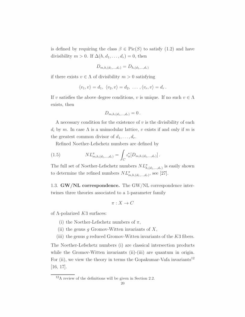
is defined by requiring the class β ∈ Pic(S) to satisfy (1.2) and have

divisibility m > 0. If ∆(h, d1, . . . , dr) = 0, then

Dm,h,(d1,...,dr) = Dh,(d1,...,dr)

if there exists v ∈ Λ of divisibility m > 0 satisfying

〈v1, v〉 = d1, 〈v2, v〉 = d2, . . . , 〈vr, v〉 = dr .

If v satisfies the above degree conditions, v is unique. If no such v ∈ Λ

exists, then

Dm,h,(d1,...,dr) = 0 .

A necessary condition for the existence of v is the divisibility of each

di by m. In case Λ is a unimodular lattice, v exists if and only if m is

the greatest common divisor of d1, . . . , dr.

Refined Noether-Lefschetz numbers are defined by

(1.5) NLπm,h,(d1,...,dr) =

∫

C

ι∗π[Dm,h,(d1,...,dr)] .

The full set of Noether-Lefschetz numbers NLπh,(d1,...,dr) is easily shown

to determine the refined numbers NLπm,h,(d1,...,dr), see [27].

1.3. GW/NL correspondence. The GW/NL correspondence inter-

twines three theories associated to a 1-parameter family

π : X → C

of Λ-polarized K3 surfaces:

(i) the Noether-Lefschetz numbers of π,

(ii) the genus g Gromov-Witten invariants of X ,

(iii) the genus g reduced Gromov-Witten invariants of theK3 fibers.

The Noether-Lefschetz numbers (i) are classical intersection products

while the Gromov-Witten invariants (ii)-(iii) are quantum in origin.

For (ii), we view the theory in terms the Gopakumar-Vafa invariants12

[16, 17].

12A review of the definitions will be given in Section 2.2.20

Let nXg,(d1,...,dr) denote the Gopakumar-Vafa invariant of X in genus

g for π-vertical curve classes of degrees13 d1, . . . , dr with respect to

the line bundles L1, . . . , Lr. Let rg,β denote the reduced K3 invariant

defined in Section 0.3 for an effective curve class β. Since rg,β depends

only upon the divisibility m and the norm square

〈β, β〉 = 2h− 2 ,

we will use the more efficient notation

rg,m,h = rg,β .

The following result is proven14 in [35] by a comparison of the reduced

and usual deformation theories of maps of curves to the K3 fibers of

π.

Theorem 3. For degrees (d1, . . . , dr) positive with respect to the quasi-

polarization λπ,

nXg,(d1,...,dr) =∞∑

h=0

∞∑

m=1

rg,m,h ·NLπm,h,(d1,...,dr) .

For fixed g and (d1, . . . , dr), the sum over m is clearly finite since

m must divide each di. The sum over h is also finite since, for fixed

(d1, . . . , dr), NLπm,h,(d1,...,dr)

vanishes for sufficiently high h by Proposi-

tion 3 of [35]. By Lemma 2 of [35], rg,m,h vanishes for h < 0 (and is

therefore omitted from the sum in Theorem 3).

2. Anticanonical K3 surfaces in P2 × P1

2.1. Polarization. Let P2 × P1 be the blow-up of P2 × P1 at a point,

P2 × P1 → P2 × P1 .

The Picard group is of rank 3:

Pic(P2 × P1) ∼= ZL1 ⊕ ZL2 ⊕ ZE ,

13The invariant nXg,(d1,...,dr)

may be a (finite) sum of nXg,γ for π-vertical curve

classes γ ∈ H2(X,Z).14The result of the [35] is stated in the rank r = 1 case, but the argument is

identical for arbitrary r.21

where L1 and L2 are the pull-backs of O(1) from the factors P2 and P1

respectively and E is the exceptional divisor. The anticanonical class

3L1 + 2L2 − 2E is base point free.

A nonsingular anticanonical K3 hypersurface S ⊂ P2 × P1 is natu-

rally lattice polarized by L1, L2, and E. The lattice is

Λ =

2 3 03 0 00 0 −2

.

A general anticanonical Calabi-Yau 3-fold hypersurface,

X ⊂ P2 × P1 × P1 ,

determines a 1-parameter family of anticanonicalK3 surfaces in P2 × P1,

(2.1) π3 : X → P1 ,

via projection π3 onto the last P1. The fibers of π3 have at worst nodal

singularities.15 The Noether-Lefschetz theory of the Λ-polarized family

(X, L1, L2, E, π3)

plays a central role in our proof of Theorem 1. The quasi-polarization

λπ3 (condition (ii) of Section 1.1) can be taken to be any very ample

line bundle on P2 × P1.

2.2. BPS states. Let (X, L1, L2, E, π3) be the Λ-polarized family of

anticanonical K3 surfaces of P2 × P1 defined in Section 2.1. The verti-

cal classes are the kernel of the push-forward map by π3,

0 → H2(X,Z)π3 → H2(X,Z) → H2(P

1,Z) → 0 .

Let Mg(X, γ) be the moduli space of stable maps from connected

genus g curves to X of class γ. Gromov-Witten theory is defined by

integration against the virtual class,

(2.2) NX

g,γ =

∫

[Mg(X,γ)]vir1 .

The expected dimension of the moduli space is 0.

15There are 192 nodal fibers. We leave the elementary classical geometry hereto the reader.

22

The full genus Gromov-Witten potential FX for nonzero vertical

classes is the series

FX =∑

g≥0

∑

06=γ∈H2(X,Z)π3

NX

g,γ λ2g−2vγ ,

where v is the curve class variable. The BPS counts nX

g,γ of Gopakumar

and Vafa are uniquely defined by the following equation:

FX =∑

g≥0

∑

06=γ∈H2(X,Z)π3

nX

g,γλ2g−2

∑

d>0

1

d

(sin(dλ/2)

λ/2

)2g−2

vdγ .

Conjecturally, the invariants nX

g,γ are integral and obtained from the

cohomology of an as yet unspecified moduli space of sheaves on X . We

do not assume the conjectural properties hold.

Using the Λ-polarization, we label the classes γ ∈ H2(X,Z)π3 by their

pairings with Li and E,

γ 7→(∫

γ

[L1],

∫

γ

[L2],

∫

γ

[E]

).

We write the BPS counts as nX

g,(d1,d2,d3). Since γ 6= 0, not all the di can

vanish.

2.3. Invertibility of constraints. Let P ⊂ Z3 be the set of triples

(d1, d2, d3) 6= (0, 0, 0) which are positive with respect to the quasi-

polarization λπ3 of the Λ-polarized family

π3 : X → P1 .

Theorem 3 applied to (X, L1, L2, E, π3) yields the equation

(2.3) nX

g,(d1,d2,d3)=

∞∑

h=0

∞∑

m=1

rg,m,h ·NLπ3m,h,(d1,d2,d3)

for (d1, d2, d3) ∈ P. We view (2.3) as linear constraints for the un-

knowns rg,m,h in terms of the BPS states on the left and the refined

Noether-Lefschetz degrees.

The integrals rg,m,h are very simple in case h ≤ 0. By Lemma 2 of

[35], rg,m,h = 0 for h < 0,

r0,1,0 = 1 ,

and rg,m,0 = 0 otherwise.23

Proposition 1. The set of invariants rg,m,hg≥0,m≥1,h>0 is uniquely

determined by the set of constraints (2.3) for (d1, d2, d3) ∈ P and the

integrals rg,m,h≤0.

Proof. A certain subset of the linear equations will be shown to be

upper triangular in the variables rg,m,h.

Let us fix in advance the values of g ≥ 0, m ≥ 1, and h > 0. We

proceed by induction on h assuming the reduced invariants rg,m′,h′ have

already been determined for all h′ < h. If 2h − 2 is not divisible by

2m2, then we have rg,m,h = 0 by definition, so we can further assume

2h− 2 = m2(2s− 2)

for an integer s > 0.

Consider the fiber class γ ∈ H2(X,Z)π3 given by the lattice element

msL1 +mL2 +m(s+ 1)E,

γ =(ms[L1] +m[L2] +m(s + 1)[E]

)∩ [S] ,

where S is a K3-fiber of π3. Since L1, L2 and E are effective on S,

the class γ is effective and hence positive with respect to the quasi-

polarization of Λ. The degrees of γ are

(2.4) (d1, d2, d3) = (2ms+ 3m, 3ms,−2m(s+ 1)) ,

and γ is of divisibility exactly m in the lattice Λ.

Consider equation (2.3) for (d1, d2, d3) given by (2.4). By the Hodge

index theorem, we must have

0 ≤ ∆(h′, 2ms+ 3m, 3ms,−2m(s+ 1))(2.5)

= 18(2− 2h′ +m2(2s− 2))

= 36(h− h′)

if NLπ3m′,h′,(2ms+3m,3ms,−2m(s+1)) 6= 0. Inequality (2.5) implies h′ ≤ h. If

h′ = h, then

∆(h′ = h, 2ms+ 3m, 3ms,−2m(s+ 1)) = 0 .

By the definition of Section 1.2.3,

NLπ3m′,h′=h,(2ms+3m,3ms,−2m(s+1)) = 024

unless there exists v ∈ Λ of divisibility m′ with degrees

(2ms+ 3m, 3ms,−2m(s+ 1)) .

But γ ∈ Λ is the unique such lattice element, and γ has divisibility m.

Therefore, the constraint (2.3) takes the form

nXg,(2ms+3m,3ms,−2m(s+1)) = rg,m,hNLπ3m,h,(2ms+3m,3ms,−2m(s+1)) + . . . ,

where the dots represent terms involving rg,m′,h′ with h′ < h. The

leading coefficient is given by

NLπ3m,h,(2ms+3m,3ms,−2m(s+1)) = NLπ3h,(2ms+3m,3ms,−2m(s+1)) = −2 .

As the system is upper-triangular, we can invert to solve for rg,m,h.

The calculation of NLπ3h,(2ms+3m,3ms,−2m(s+1) is elementary. In the

discriminant ∆ = 0 case, we must determine the degree of the dual

of the Hodge line bundle K on the base P1. The relative dualizing

sheaf ωπ3 is the pull-back of OP1(2) from the base. Hence, the dual of

the Hodge line has degree −2. See Section 6.3 of [35] for many such

calculations.

The proof of Proposition 1 does not involve induction on the genus.

The same argument will be used later in the theory of stable pairs.

3. Theorem 2

3.1. Strategy. We will prove Theorem 2 via the GW/P and Noether-

Lefschetz correspondences for the family (X, L1, L2, E, π3) of K3 sur-

faces of defined in Section 2.1. While all of the necessary Gromov-

Witten theory has been established in Sections 1 and 2, our proof here

depends upon stable pairs results proven later in Sections 7 and 8.

3.2. Stable pairs. Let V be a nonsingular, projective 3-fold, and let

β ∈ H2(V,Z) be a nonzero class. We consider the moduli space of

stable pairs

[OVs→ F ] ∈ Pn(V, β)

25

where F is a pure sheaf supported on a Cohen-Macaulay subcurve of

V , s is a morphism with 0-dimensional cokernel, and

χ(F ) = n , [F ] = β .

The space Pn(V, β) carries a virtual fundamental class of dimension∫βc1(TV ) obtained from the deformation theory of complexes with triv-

ial determinant in the derived category [39].

We specialize now to the case where V is the total space of a K3-

fibration (with at worst nodal fibers),

π : V → C ,

over a nonsingular projective curve and β ∈ H2(V,Z)π is a vertical

class. Then the expected dimension of Pn(V, β) is always 0. For nonzero

β ∈ H2(V,Z)π, define the stable pairs invariant

N•n,β =

∫

[Pn(V,β)]vir1 .

The partition function is

ZP

(V ; q

)β=∑

n

N•n,β q

n.

Since Pn(V, β) is empty for sufficiently negative n, the partition func-

tion is a Laurent series in q. The following is a special case of Conjecture

3.26 of [39].

Conjecture 3. The partition function ZP

(V ; q)β is the Laurent expan-

sion of a rational function in q.

If the total space V is a Calabi-Yau 3-fold, then Conjecture 3 has

been proven in [6, 44]. In particular, Conjecture 3 holds for the anti-

canonical 3-fold

X ⊂ P2 × P1 × P1

of Section 2.1.

In fact, if V is any complete intersection Calabi-Yau 3-fold in a toric

variety which admits sufficient degenerations, Conjecture 3 has been

proven in [38]. By factoring equations, there is no difficulty in con-

structing the degenerations of X into toric 3-folds required for [38].26

Just as in the case of the quintic in P4, the geometries which occur are

toric 3-folds, projective bundles over K3 and toric surfaces, and fibra-

tions over curves. A complete discussion of the degeneration scheme

for X is given in Appendix B.

3.3. GW/P correspondence for X. Following the notation of Sec-

tion 2.2, let H2(X,Z)π3 denote the vertical classes of X and let

FX =∑

g≥0

∑

06=γ∈H2(X,Z)π3

NX

g,γ λ2g−2vγ

be the potential of connected Gromov-Witten invariants. The parti-

tion function (of possibly disconnected) Gromov-Witten invariants is

defined via the exponential,

ZGW

(X;λ

)= exp

(FX).

Let ZGW

(X;λ

)γdenote the coefficient of vγ in ZGW

(X;λ

). The main re-

sult of [38] applied to X is the following GW/P correspondence for com-

plete intersection Calabi-Yau 3-folds in products of projective spaces.

GW/P correspondence. After the change of variable −q = eiλ, we

have

ZGW

(X;λ

)γ= ZP

(X; q)γ.

The change of variables is well-defined by the rationality of ZP

(X; q)γ

of Conjecture 3. The GW/P correspondence is proven in [38] for every

non-zero class in H2(X,Z), but we only will require here the statement

for fiber classes γ.

3.4. K3 integrals. Let S be a nonsingular projective K3 surface with

a nonzero class α ∈ Pic(S) which is both effective and primitive. By

the definitions of Sections 0.3 in Gromov-Witten theory,

Fα =∑

g≥0

∑

m>0

Rg,mα λ2g−2vmα,

27

Fα =∑

g≥0

∑

m>0

rg,mα λ2g−2

∑

d>0

1

d

(sin(dλ/2)

λ/2

)2g−2

vdmα.

Via K3-fibrations over a pointed curve

ǫ : T → (∆, 0)

satisfying the conditions (i), (ii), and (⋆) of Section 0.5, we have defined

in (0.8) the series

Fα =∑

n∈Z

∑

m>0

Rn,mα qnvmα

in the theory of stable pairs. Using the identity

22g−2sin(dλ/2)2g−2 =

(eidλ/2 − e−idλ/2

i

)2g−2

= (−1)g−1((−q)d − 2 + (−q)−d

)g−1

under the change of variables −q = eiλ, we define the stable pairs BPS

invariants rg,mα by the relation

Fα =∑

g∈Z

∑

m>0

rg,mα∑

d>0

(−1)g−1

d

((−q)d − 2 + (−q)−d

)g−1vdmα .

See Section 3.4 of [39] for a discussion of such BPS expansions for stable

pairs. The invariants rg,mα are integers.

Since rg,β depends only upon the divisibility m and the norm square

〈β, β〉 = 2h− 2 ,

we will use, as before, the notation

rg,m,h = rg,β .

By definition in Gromov-Witten theory, rg,m,h = 0 for g < 0. However

for fixed m and h, the definitions allow rg,m,h to be nonzero for all

positive g. On the stable pairs side for fixed m and h, rg,m,h = 0 for

sufficiently large g, but rg,m,h may be nonzero for all negative g.

We will prove Theorem 2 by showing the BPS counts for K3 surfaces

in Gromov-Witten theory and stable pairs theory exactly match:

(3.1) rg,m,h = rg,m,h

for all g ∈ Z, m ≥ 1, and h ∈ Z.28

3.5. Noether-Lefschetz theory for stable pairs. The stable pairs

potential FX for nonzero vertical classes is the series

FX = log

1 +

∑

06=γ∈H2(X,Z)π3

ZP

(X; q)γvγ

,

where v is the curve class variable. The stable pairs BPS counts nX

g,γ

are uniquely defined by

FX =∑

g∈Z

∑

06=γ∈H2(X,Z)π3

nX

g,γ

∑

d>0

(−1)g−1

d

((−q)d − 2 + (−q)−d

)g−1vdγ ,

following Section 3.4 of [39].

The following stable pairs result is proven in Section 8. A central

issue in the proof is the translation of the Noether-Lefschetz geometry

of stable pairs to a precise relation constraining the logarithm FX of

the stable pairs series.

Theorem 4. For degrees (d1, d2, d3) positive with respect to the quasi-

polarization of the family π3 : X → P1,

nX

g,(d1,d2,d3)=

∞∑

h=0

∞∑

m=1

rg,m,h ·NLπ3m,h,(d1,d2,d3) .

3.6. Proof of Theorem 2. We first match the BPS counts of X by

using the GW/P correspondence. Then, the uniqueness statement of

Proposition 1 implies (3.1).

Proposition 2. For all g ∈ Z and all γ ∈ H2(X,Z)π3, we have

nX

g,γ = nX

g,γ .

Proof. By Corollary 6 of Section 7, rg,m,h = 0 if g < 0. Theorem 4 then

implies nX

g,γ = 0 if g < 0. Hence, there are only finitely many nonzero

BPS states16 for fixed γ since nX

g,γ vanishes for sufficiently large g by

construction [39]. By the GW/P correspondence, the nX

g,γ then yield

the Gromov-Witten BPS expansion.

16The GW/P correspondence yields an equality of partition functions after thevariable change −q = eiλ whether or not ng<0,γ vanishes. Proposition 2 asserts athe stronger result: the Gromov-Witten BPS expansion equals the stable pairs BPSexpansion. Since these expansions are in opposite directions, finiteness is needed.

29

Proposition 3. For all g ∈ Z, m ≥ 1, and h ∈ Z, we have

rg,m,h = rg,m,h .

Proof. The equality rg,m,h = rg,m,h holds in case h ≤ 0 by following the

argument of Lemma 2 of [35] for stable pairs.17 For h < 0, the vanishing

of rg,m,h holds by the same geometric argument given in Lemma 2 of

[35]. The h = 0 case is the conifold for which the equality is well known

(and a consequence of GW/P correspondence).

We view relation (2.3) and Theorem 4 as systems of linear equations

for the unknowns rg,m,h and rg,m,h respectively. By Proposition 2, we

have

nXg,γ = nXg,γ

for all g. Hence, the two systems of linear equations are the same.

We now apply the uniqueness established in Proposition 1. The

initial conditions and the linear equations are identical. Therefore the

solutions must also agree.

Theorem 2 follows immediately from Proposition 3 for the K3 in-

variants in Gromov-Witten theory and stable pairs.

4. K3× C: Localization

4.1. Overview. We begin now our analysis of the moduli spaces of

stable pairs related to K3 surfaces and K3-fibrations. Let S be a

nonsingular projective K3 surface. We first study the trivial fibration

Y = S × C −→ C

by C∗-localization with respect to the scaling action on C. Let t denote

the weight 1 representation of C∗ on the tangent space to C at 0 ∈ C.

We compute here the C∗-residue contribution to the reduced sta-

ble pairs theory of S × C of the C∗-fixed component18 parameterizing

stable pairs supported on S and thickened uniformly k times about

17A different argument is given in Corollary 5 of Section 7.18Throughout we use the term component to denote any open and closed subset.

More formally, a component for us is a union of connected components in thestandard sense.

30

0 ∈ C. In Section 5, all other C∗-fixed components will be shown to

have vanishing contributions to the virtual localization formula.

4.2. Uniformly thickened pairs. Define the following Artinian rings

and schemes:

(4.1) Ak = C[x]/(xk) , Bk = SpecAk .

We have the obvious maps

SpecC Bkπk

oo

ιk// C = SpecC[x] .

For any variety Z, we define

Zk = Z × Bk ,

and use the same symbols πk, ιk to denote the corresponding projections

and inclusions,

(4.2) Z Zkπkoo

ιk// Z × C .

We will often abbreviate ιk to ι.

Let β ∈ H2(S,Z) be a curve class. Let PS = Pn(S, β) denote the

moduli space of stable pairs on S with universal stable pair (F, s) and

universal complex

I•S =OS×PS

s−→ F.

Using the maps (4.2) for Z = S × PS (so Z × C = Y × PS) we define

(4.3) Fk = π∗kF, I•Sk

=OSk×PS

sk−→ Fk

on Sk × PS, where sk = π∗ks. Pushing sk forward to Y × PS we obtain

(4.4) I•Y =OY×PS

sk−→ ι∗Fk.

Since we have constructed a flat family over PS of stable pairs on Y

of class19 kβ and holomorphic Euler characteristic kn, we obtain a

classifying map from PS to the moduli space of stable pairs on Y :

(4.5) f : PS = Pn(S, β) // Pkn(Y, kβ) = PY .

Lemma 1. The map (4.5) is an isomorphism onto an open and closed

component of the C∗-fixed locus of PY .

19For any class γ ∈ Pic(S), we denote the push-forward to H2(Y,Z) also by γ.31

Proof. Let Pf denote the open and closed component of (PY )C∗

con-

taining the image of f . Certainly, f is a bijection on closed points onto

Pf . There is a C∗-fixed universal stable pair on Y ×Pf . We push down

the universal stable pair to S×Pf and then take C∗-invariant sections.

The result is flat over Pf and hence classified by a map Pf → PS which

is easily seen to be the inverse map to f .

4.3. Deformation theory of pairs. Let PY = Pm(Y, γ) be the mod-

uli space of stable pairs on Y of class γ ∈ H2(Y,Z) with holomorphic

Euler characteristic m. There is a universal complex I•Y over Y × PY .

We will soon take m = kn and γ = kβ, in which case I•Y pulls back via

the classifying map f : PS → PY to (4.4).

We review here the basics of the deformation theory of stable pairs

on the 3-fold Y [39]. Let

πP : Y × PY → PY

be the projection, and define

(4.6) E•

Y = (RHomπP (I•

Y , I•

Y )0)∨[−1] ∼= RHomπP (I

•

Y , I•

Y ⊗ ωπP )0[2] .

Here RHomπP = RπP∗RHom, the subscript 0 denotes trace-free ho-

momorphisms, and the isomorphism is Serre duality20 down πP . Let

L denote the truncated cotangent complex τ≥−1L•. Using the Atiyah

class of I•Y , we obtain a map [39, Section 2.3],

(4.7) E•

Y −→ LPY,

exhibiting E•

Y as a perfect obstruction theory for PY [19, Theorem 4.1].

In fact, (4.7) is the natural obstruction theory of trivial-determinant

objects I• = OYs→ F of the derived category D(Y ). The more

natural obstruction theory of pairs (F, s) is given by the complex21

(4.8) (RHomπP (I•

Y ,FY ))∨

20Although πP is not proper, the compact support of RHom(I•Y , I•

Y )0 ensuresthat Serre duality holds. This is proved in [36, Equations 15,16], for instance, bycompactifying Y = S × C to Y = C× P1.

21This is essentially proved in [20] once combined with [3, Theorem 4.5], see [21,Sections 12.3-12.5] for a full account.

32

where FY is the universal sheaf. However (4.8) is not perfect in general.

To define stable pair invariants, we must use (4.6). The two theories

give the same tangent spaces, but different obstructions. On surfaces,

however, the analogous obstruction theory

(4.9) E•

S = (RHomπP (I•

S,F))∨

is indeed perfect and is used to define invariants [28]. Here πP denotes

the projection S × PS → PS.

The following result describes the relationship between the above

obstruction theories when pulled-back via the map f : PS → PY of

(4.5).

Proposition 4. We have an isomorphism

f ∗E•

Y∼= E•

S ⊗A∗k ⊕ (E•

S)∨⊗t−1Ak[1] ,

where22 A∗k = 1 + t + . . .+ tk−1 and t−1Ak = t−1 + t−2 + . . .+ t−k.

Proof. We will need two preliminaries on pull-backs. First, over Sk×PSthere is a canonical exact triangle

(4.10) Fk ⊗N∗k [1] −→ ι∗ι∗Fk −→ Fk ,

where ι∗ = Lι∗k is the derived pull-back functor, and

Nk∼= OSk×PS

⊗ tk

denotes the normal bundle of Sk ×PS in Y ×PS. Second, combine the

first arrow of (4.10) with the obvious map OY×PS→ ι∗OSk×PS

:

RHom(ι∗Fk,OY×PS) −→ RHom(ι∗Fk, ι∗OSk×PS

)

∼= ι∗RHom(ι∗ι∗Fk,OSk×PS) −→ ι∗RHom(Fk ⊗N∗

k [1],OSk×PS) .

A local computation shows the above composition is an isomorphism:

(4.11) RHom(ι∗Fk,OY×PS) ∼= ι∗RHom(Fk ⊗N∗

k [1],OSk×PS) .

Now combine (4.10) with ι∗ of the triangle

(4.12) I•Y → OY×PS→ ι∗Fk

22We ignore here the ring structure (4.1) on Ak and considering Ak as just avector space with C∗-action. As such, A∗

k∼= tk−1Ak, as we use below.

33

to give the following diagram of exact triangles on Sk × PS:

(4.13) ι∗I•Y

OSk×PS

OSk×PS

Fk ⊗N∗k [1]

// ι∗ι∗Fk // Fk .

The right hand column defines the complex I•Sk(4.3), so by the octa-

hedral axiom we can fill in the top row with the exact triangle

(4.14) Fk ⊗N∗k −→ ι∗I•Y −→ I•Sk

.

Again letting πP denote both projections

Sk × PS → PS and Y × PS → PS ,

we apply RHomπP (I•

Y , · ) to I•Y → OY×PS→ ι∗Fk to give the triangle

(4.15)

RHomπP (I•

Y , ι∗Fk) −→ RHomπP (I•

Y , I•

Y )[1] −→ RHomπP (I•

Y ,O)[1]

relating the obstruction theory (4.8) to the obstruction theory (4.6)

(without its trace-part removed: we will deal with this presently).

Now use the following obvious diagram of exact triangles on Y ×PS:

I•Y //

OY×PS//

ι∗Fk

ι∗I•Sk

// ι∗OSk×PS// ι∗Fk .

This maps the triangle (4.15) to the triangle

RHomπP (I•

Y , ι∗Fk)−→RHomπP (I•

Y , ι∗I•

Sk)[1]−→RHomπP (I

•

Y , ι∗O)[1].

By adjunction this is

RHomπP (ι∗I•Y ,Fk)−→RHomπP (ι

∗I•Y , I•

Sk)[1]−→RHomπP (ι

∗I•Y ,O)[1],

which in turn maps to

(4.16)

RHomπP (Fk,Fk)tk−→RHomπP (Fk, I

•

Sk)tk[1]−→RHomπP (Fk,O)tk[1]

34

by the first arrow Fk ⊗N∗k → ι∗I•Y of (4.14). Notice that since I•Sk

and

Fk are the pull-backs of I•S and F by πk : Sk → S, the central term

simplifies to

RHomπP (F, I•

S)⊗ tkAk[1] ∼= E•

S ⊗ tkAk[−1] ,

where E•

S is the obstruction theory (4.9).

We next remove the trace component of (4.15) using the diagram

(4.17) RπP∗OY×PS[1]

id

RπP∗OY×PS[1]

RHomπP (I•

Y , ι∗Fk) // RHomπP (I•

Y , I•

Y )[1]//

RHomπP (I•

Y ,O)[1]

RHomπP (I•

Y , I•

Y )0[1]// RHomπP (ι∗Fk,O)[2] .

Here the right hand column is given by applying RHomπP ( · ,O) to

(4.12). The top right hand corner commutes because the composition

O id−→ Hom(I•Y , I•

Y ) → Hom(I•Y ,O) takes 1 to the canonical map

I•Y → O. Therefore the whole diagram commutes.

The central row of (4.17) is (4.15), and our map from (4.15) to

(4.16) kills the top row of (4.17) by C∗-equivariance: RπP∗OY×PS[1]

has C∗-weights in (−∞, 0] while (4.16) has weights in [1, k]. Therefore

it descends to a map from the bottom row of (4.17) (completed using

the octahedral axiom) to (4.16). The upshot is the following map of

triangles

(4.18)

RHomπP (I•

Y , ι∗Fk) //

f ∗(E•

Y )∨ //

RHomπP (ι∗Fk,O)[2]

RHomπP (Fk,Fk)tk // E•

S ⊗ tkAk[−1] // RHomπP (Fk,O)tk[1] .

Recall that the first column was induced from the triangle (4.14) so

sits inside a triangle

RHomπP (I•

Sk,Fk) −→ RHomπP (I

•

Y , ι∗Fk) −→ RHomπP (Fk,Fk)tk .

35

Again we can simplify because I•Skand Fk are the pull-backs of I•S and

F by πk : Sk → S. That is,

RHomπP (I•

Y , ι∗Fk) ∼= RHomπP (I•

S,F)⊗Ak ⊕ RHomπP (F,F)⊗tkAk ,

where the splitting follows from the C∗-invariance of the connecting

homomorphism: it must vanish because Ak has weights in [−(k−1), 0]

while tkAk has weights in [1, k].

So this splits the first vertical arrow of (4.18); we claim the last

vertical arrow is the isomorphism induced by (4.11). Altogether this

gives the splitting

f ∗(E•

Y )∨ ∼= RHomπP (I

•

S,F)⊗ Ak ⊕ E•

S[−1]⊗ tkAk .

Dualizing gives

f ∗E•

Y∼= E•

S ⊗ A∗k ⊕ (E•

S)∨[1]⊗ t

−1Ak ,

as required.

It remains to prove the claim that the third vertical arrow of (4.18)

is induced by (4.11). By the construction of these maps, it is sufficient

to prove the commutativity of the diagram

RHomπP (I•

Y ,OY×PS) //

∂∗

RHomπP (Fk ⊗N∗k ,OSk×PS

)

RHomπP (ι∗Fk[−1],OY×PS) .

∼

22

Here the vertical arrow is induced by the connecting homomorphism ∂

of the standard triangle I•Y → OY×PS→ ι∗Fk, and the diagonal arrow

is RπP∗ applied to (4.11).

The horizontal arrow is our map from (4.15) to (4.16) (restricted to

the right hand term in each triangle). It is therefore the composition

RHomπP (I•

Y ,OY×PS) −→ RHomπP (I

•

Y , ι∗OSk×PS)

∼= RHomπP (ι∗I•Y ,OSk×PS

)(4.14)−→ RHomπP (Fk ⊗N∗

k ,OSk×PS) .

Via ∂ : ι∗Fk[−1] → I•Y , the above composition maps to the composition

RHomπP (ι∗Fk[−1],OY×PS) −→ RHomπP (ι∗Fk[−1], ι∗OSk×PS

)

∼= RHomπP (ι∗ι∗Fk[−1],OSk×PS

)(4.10)−→ RHomπP (Fk ⊗N∗

k ,OSk×PS) .

36

Therefore the first two resulting squares commute. The last square is:

RHomπP (ι∗I•Y ,OSk×PS

)(4.14)

//

ι∗∂∗

RHomπP (Fk ⊗N∗k ,OSk×PS

)

RHomπP (ι∗ι∗Fk[−1],OSk×PS

)(4.10)

// RHomπP (Fk ⊗N∗k ,OSk×PS

) .

By the construction of (4.14) from (4.10), the square commutes.

A virtual class on Pkn(Y, kβ)C∗

induced by (E•

Y )fix is defined in [18].

The moduli space Pn(S, β) hence carries several virtual classes:

(i) via the intrinsic obstruction theory E•

S,

(ii) via (E•

Y )fix and the local isomorphism

f : Pn(S, β) −→ Pkn(Y, kβ)C∗

for every k ≥ 1.

Proposition 5. The virtual classes on Pn(S, β) obtained from (i) and

(ii) are all equal.

Proof. By Proposition 4, there is an isomorphism,

(4.19) f ∗(E•

Y )fix ∼= E•

S ,

in the derived category. Since the virtual class is expressed in terms

of the Fulton total Chern class of Pn(S, β) and the Segre class of the

dual of the obstruction theory23, the isomorphism (4.19) implies the

equality of the virtual classes.

In fact Proposition 5 is trivial: the virtual classes of Pn(S, β) ob-

tained from the obstruction theories E•

S and (E•

Y )fix both vanish by the

existence of the reduced theory.

The reduced obstruction theory for Y is constructed in, for instance,

[36, Section 3]. We review the construction in a slightly more general

setting in Section 6.6. For the reduced theory of S, we can either C∗-

localize the 3-fold reduced class, or equivalently, use the construction in

[28]. In particular, Proposition 3.4 of [28] shows the two constructions

23The relationship of the virtual class with the Fulton total Chern class and thenormal cone is reviewed in Appendix C.1.

37

are compatible under the isomorphism (4.5). They both remove a

trivial piece OP [−1] (of C∗-weight 0!) from the obstruction theory.

The nontrivial version of Proposition 5 is the following.

Proposition 6. The reduced virtual classes on Pn(S, β) obtained from

(i) and (ii) are all equal.

The proof of Proposition 6 is exactly the same as the proof of Propo-

sition 5 given above.

4.4. Localization calculation I. We can now evaluate the residue

contribution of the locus of k-times uniformly thickened stable pairs

Pn(S, β) ⊂ Pkn(Y, kβ)C∗

of (4.5) to the C∗-equivariant integral∫

[Pkn(Y,kβ)]redC∗

1 .

We will see in Section 5 that the contributions of all other C∗-fixed loci

to the virtual localization formula vanish.

By Proposition 6, the reduced virtual class on Pkn(Y, kβ)C∗

obtained

from (E•

Y )fix matches the reduced virtual class of Pn(S, β) obtained

from the obstruction theory E•

S. The virtual normal bundles are the

same for the reduced and standard obstruction theories (since the

semiregularity map is C∗-invariant here).

Writing Ak as C⊕t−1Ak−1, we can read off the virtual normal bundle

to Pn(S, β) ⊂ Pkn(Y, kβ) from Proposition 4:

Nvir = (E•

S)∨⊗ t−1Ak−1 ⊕ E•

S⊗ tA∗k[−1] .

After writing tA∗k as tA

∗k−1⊕ tk, the residue contribution of Pn(S, β) to

the C∗-equivariant integral∫[Pkn(Y,kβ)]

redC∗

1 is

∫

[Pn(S,β)]red

1

e(Nvir)=

∫

[Pn(S,β)]red

e(E•

S ⊗ tA∗k−1

)

e((E•

S ⊗ tA∗k−1)

∨) e(E•

S ⊗ tk).

The rank of E•

S is the virtual dimension

〈β, β〉+ n = 2hβ − 2 + n38

of Pn(S, β) before reduction. Therefore, the rank of tensor product

E•

S⊗ tA∗k−1 is (k−1)(2hβ−2+n), and the quotient in the integrand is

(−1)(k−1)(2hβ−2+n) = (−1)(k−1)n .

Let t denote the C∗-equivariant first Chern class of the representation

t. We have proven the following result.

Proposition 7. The residue contribution of

Pn(S, β) ⊂ Pkn(Y, kβ)C∗

to the integral∫[Pkn(Y,kβ)]

redC∗

1 is:

∫

[Pn(S,β)]red

1

e(Nvir)= (−1)(k−1)n

∫

[Pn(S,β)]rede(E•

S ⊗ tk)

=(−1)(k−1)n

kt

∫

[Pn(S,β)]redc〈β,β〉+n+1(E

•

S) .

4.5. Dependence. Let S be a K3 surface equipped with an ample

primitive polarization L. Let β ∈ Pic(S) be a positive class with

respect to L,

〈L, β〉 > 0 .

If β is nonzero and effective, β must be positive. The integral

(4.20)

∫

[Pn(S,β)]redc〈β,β〉+n+1(E

•

S)

is deformation invariant as (S, β) varies so long as β remains an alge-

braic class. Hence, the integral depends only upon n, the divisibility

of β, and 〈β, β〉.If β is effective, then H2(S, β) = 0 otherwise −β would also be

effective by Serre duality. Hence, by the results of [29], the integral

(4.20) depends only upon n and

〈β, β〉 = 2hβ − 2

in the effective case.

If β is effective and hβ < 0, then the integral vanishes since the

virtual number of sections of β is negative. A proof is given below39

in Section 4.6 following [28, 29]. Finally, if hβ ≥ 0, then β must be

effective (since β is positive) by Riemann-Roch.

If β is not effective, then the integral (4.20) vanishes. In the ineffec-

tive case, hβ < 0 must hold. The discussion of cases is summarized by

the following result, whose final statement will be proved in Proposition

9 below.

Proposition 8. For a positive class β ∈ Pic(S), the integral

(4.21)

∫

[Pn(S,β)]redc〈β,β〉+n+1(E

•

S)

depends only upon n and hβ. Moreover, if hβ < 0, the integral vanishes.

4.6. Vanishing. Let S be an K3 surface with an effective curve class

β ∈ Pic(S) satisfying

β2 = 2h− 2 with h < 0 .

Let Pβ be the linear system of all curves of class β. Since h is the

reduced virtual dimension of the moduli space

P1−h(S, β) = Pβ ,

the corresponding virtual cycle vanishes,

(4.22) [P1−h(S, β)]red = 0 .

We would like to conclude

(4.23) [P1−h+k(S, β)]red = 0

for all k.

If k < 0, then P1−h+k(S, β) is empty, so (4.23) certainly holds. If

k > 0, the moduli space P1−h+k(S, β) fibers over P1−h(S, β):

P1−h+k(S, β) ∼= Hilbk(C/Pβ) π−→ Pβ ∼= P1−h(S, β) ,

where C → Pβ is the universal curve. By [1] and [28, Footnote 22], the

projection π is flat of relative dimension n. Therefore, the vanishing

(4.23) follows from (4.22) and Proposition 9 below.24 Since π is flat,

24The result was implicit in [28] but never actually stated there, so we providea proof. The result holds more generally for any surface S and class β ∈ H2(S,Z)for which H2(L) = 0 whenever c1(L) = β.

40

pull-back is well defined on algebraic cycles. Also, as we have noted, β

effective implies H2(S, β) = 0.

Proposition 9. For H2(S, β) = 0 and k ≥ 0, we have

[P1−h+k(S, β)]red = π∗[P1−h(S, β)]

red .

Proof. In [28, Appendix A], the moduli space P1−h+k(S, β) is described

by equations as follows.25 Let A be a sufficiently ample divisor on S.

The inclusion,

Pβ ⊂ Pβ+A ,

is described as the zero locus of a section of a vector bundle E. Next,

(4.24) Hilbk(C/Pβ) ⊂ Pβ ×Hilbk S

is described as the zero locus of a section of a bundle F which extends

to Pβ+A ×Hilbk S.

Let A denote the nonsingular ambient space Pβ+A × Hilbk S which

contains our moduli space

P = P1−h+k(S, β) ∼= Hilbk(C/Pβ) .

The above description then defines a natural virtual cycle on P via

(4.25) [P ]red =[s(P ⊂ A)c(π∗E)c(F ) ∩ [P ]

]h+k

,

the refined top Chern class of π∗E ⊕ F on P . Here,

h+ k = dimA− rankE − rankF

is the virtual dimension of the construction. By the main result of [28,

Appendix A], the class (4.25) is, as the notation suggests, equal to the

reduced virtual cycle of P .

By [1] and [28, Footnote 22], the section of F cutting out (4.24) is

in fact regular. Hence, the resulting normal cone

CP⊂Pβ×Hilbk S∼= F

25Since H1(S,OS) = 0 the description here is simpler.41

is locally free and isomorphic to F . We have the following exact se-

quence of cones26 :

0 −→ CP⊂Pβ×Hilbk S −→ CP⊂A −→ π∗CPβ⊂Pβ+A−→ 0 .

After substitution in (4.25), we obtain

[P ]red =[s(F )π∗s

(Pβ ⊂ Pβ+A

)π∗c(E)c(F ) ∩ π∗

[Pβ]]h+n

= π∗([s(Pβ ⊂ Pβ+A

)c(E) ∩

[Pβ]]h

)

= π∗[Pβ]red

.

5. K3× C: Vanishing

5.1. Overview. We will show the components of (PY )C∗

which do not

correspond to the thickenings studied in Section 4 do not contribute to

the localization formula.

Recall first the proof of the vanishing of the ordinary (non-reduced)

C∗-localized invariants of

Y = S × C .

Translation along the C-direction in Y induces a vector field on PY

which has C∗-weight 1. By the symmetry of the obstruction theory,

such translation induces a C∗-weight 0 cosection: a surjection from

the obstruction sheaf ΩPYto OPY

. Since the cosection is C∗-fixed, it

descends to a cosection for the C∗-fixed obstruction theory on (PY )C∗

,

forcing the virtual cycle to vanish [25].

To apply the above strategy to the reduced obstruction theory, we

need to find another weight 1 vector field on the moduli space. We will

describe such a vector field which is proportional to the original trans-

lational vector field along (PY )C∗ ⊂ PY precisely on the components

of uniformly thickened stable pairs of Section 4. On the other com-

ponents of (PY )C∗

, the linear independence of the two weight 1 vector

fields forces the reduced localized invariants to vanish.

26Since H1(S,OS) = 0 and the Hilbert scheme of curves is just the nonsingularlinear system Pβ, all three terms are locally free. In general only the first is.

42

5.2. Basic model. Our new vector field will again arise from an action

in the C-direction on Y , pulling apart a stable pair supported on a

thickening of the central fiber S × 0. The S-direction plays little

role, so we start by explaining the basic model on C itself. For clarity,

we will here use the notation

Cx = SpecC[x] ,

where the subscript denotes the corresponding parameter. The space

Cx carries its usual C∗-action, with the coordinate function x having

weight −1.

Consider the k-times thickened origin Bk ⊂ Cx. We wish to fix

Bk−1 ⊂ Bk and move the remaining point away through Cx at unit

speed. In other words, we consider the flat family of subschemes of Cx

parameterized by t ∈ Ct given by

(5.1) Z = xk−1(t− x) = 0 ⊂ Cx × Ct .

Specializing to t = 0 indeed gives the subscheme xk = 0 = Bk, while

for t 6= 0 we have xk−1 = 0 ⊔ x = t.

5.3. Extension class. Consider OZ as a flat family of sheaves over

Ct defining a deformation of fiber OBkover t = 0. After restriction to

SpecC[t]/(t2), we obtain a first order deformation OZ/(t2) of the sheaf

OZ/(t) = OBk.

Such deformations are classified by an element e of the group

(5.2) Ext1Cx(OBk

,OBk)

described as follows. The exact sequence

0 −→ OZ/(t)t−→ OZ/(t

2) −→ OZ/(t) −→ 0 ,

is isomorphic to

(5.3) 0 −→ OBk

t−→ C[x, t]

(t2, xk−1(x− t))−→ OBk

−→ 0 .

43

Considering (5.3) as a sequence of C[x]-modules (pushing it down by

π2 : Cx × SpecC[t]/(t2) → Cx ) an extension class e in (5.2) is deter-

mined.

Using the resolution

0 −→ OCx(−Bk)xk−→ OCx −→ OBk

−→ 0

of OBkwe compute (5.2) as

Ext1Cx(OBk

,OBk) ∼= Hom(OCx(−Bk),OBk

)

∼= H0(OBk(Bk)) ∼= H0(OBk

)⊗ tk.(5.4)

Proposition 10. The class e ∈ Ext1Cx(OBk

,OBk) of the first order

deformation OZ/(t2) of OBk

is

xk−1 ⊗ tk ∈ H0(OBk)⊗ tk.

It coincides (to first order) with the deformation given by moving OBk

by the translational vector field 1k∂x. In particular, e has C∗-weight 1.

Proof. Consider the generator of Hom(OCx(−Bk),OBk) multiplied by

xk−1. From the description (5.4), it corresponds to the extension E

coming from the pushout diagram

(5.5) 0 // OCx(−Bk)

xk−1

xk// OCx

//

OBk// 0

0 // OBk// E // OBk

// 0 .

On the other hand, e is defined by the push-down to Cx of the extension

(5.3). The latter sits inside the diagram

0 // C[x]

xk−1

xk// C[x] //

π∗

C[x]/(xk) // 0

0 // C[x]/(xk)t

// C[x, t]/(t2, xk−1(x− t)) // C[x]/(xk) // 0 .

Here the central vertical arrow π∗ takes a polynomial in x to the same

polynomial in x (with no t-dependence). This is indeed a map of C[x]-

modules (though not C[x, t]-modules) and makes the left hand square44

commute since xk = xk−1t in the ring

OZ/(t2) = C[x, t]/(t2, xk−1(x− t)) .

Since the second diagram is isomorphic to the first diagram (5.5), we

find e is indeed xk−1 ⊗ tk.

Next we observe that moving OBkby the translation vector field 1

k∂x

yields the structure sheaf of the different family

(x− t/k)k = 0

⊂ Cx × Ct .

Restricting to SpecC[t]/(t2) gives the first order deformation

C[x, t](t2,(x− t/k

)k) =C[x, t]

(t2, xk − txk−1),

the same as OZ/(t2).

Finally, the C∗-weight of 1k∂x is clearly 1. More directly, xk−1 ⊗ tk

has weight −(k − 1) + k = 1.

The conceptual reason for the surprising result of Proposition 10 is

that, to first order, weight 1 deformations only see the corresponding

deformation of the center of mass of the subscheme. The two deforma-

tions in Proposition 10 clearly deform the center of mass in the same

way.

We will next apply a version of the above deformation to C∗-fixed

stable pairs. The first order part of the deformation will describe a

weight 1 vector field on PY along (PY )C∗ ⊂ PY and thus a C∗-invariant

cosection of the obstruction theory.

On the stable pairs which are uniformly thickened as in Section 4.2,

Proposition 10 will show the new vector field to be proportional to the

standard vector field given by the translation ∂x. Thus our cosection is

proportional to the cosection we have already reduced by, and provides

us nothing new. Hence, the nonzero contributions of Section 4.4 are

permitted.45

For non uniformly thickened stable pairs, however, the new vector

field will be seen to be linearly independent of the translational vector

field.

5.4. Full model. The basic model of Section 5.2 gives a deformation

of the C[x]-modules Ak = C[x]/(xk). We now extend this to describe

a deformation of any C∗-equivariant torsion C[x]-module M which is a

(possibly infinite) direct sum of finite dimensional C∗-equivariant C[x]-

modules. By the classification of modules over PIDs,M is a direct sum

of tj-twists of the standard modules Ak = C[x]/(xk). Since these were

treated in Section 5.2, the extension is a simple matter. However, by

describing our deformations intrinsically, we will be able to apply the

construction to C∗-fixed stable pairs (F, s) on S × Cx. Let

U ⊂ S

be an affine open set. Then, F |U×Cx is equivalent to a C∗-equivariant

torsion C[x]-module carrying an action of the ring O(U). The model

developed here will sheafify over S and determines a deformation of

(F, s).

Since the sheaf F |U×Cx has only finitely many weights (all nonposi-

tive), we restrict attention to torsion C∗-equivariant C[x]-modules M

with weights lying in the interval [−(k−1), 0] for some k ≥ 1. Examples

include Ak and Ajt−(k−j) for j ≤ k. Write

M =

k−1⊕

i=0

Mi

as a sum of weight spaces, where Mi has weight −i. Multiplication by

x is encoded in the weight (−1) operators

X : Mi −→Mi+1 .

Since X annihilates the most negative weight space, Mk−1 ⊂ M is an

equivariant C[x]-submodule. We will define a deformation which moves

Mk−1 away at unit speed while leaving the remaining M/Mk−1 fixed.

To do so, notice the basic model (5.1) of Section 5.2 can be described

as follows. Take the direct sum of the structure sheaves of the two46

irreducible components of Z (or, equivalently, the structure sheaf OZ

of the normalization of Z), then OZ is the subsheaf of sections which

agree over the intersection ∆(Bk−1) of the two components:

(5.6) OZ = ker(π∗OBk−1

⊕∆∗O(r,−r)

// ∆∗OBk−1

).

Here, ∆∗OBk−1= ∆∗Ak−1 and r denotes restriction to ∆(Bk−1). Finally

π : Cx × Ct −→ Cx ,

∆: C −→ Cx × Ct

are the projection and the inclusion of the diagonal respectively.

We define the C∗-equivariant C[x, t]-module M to be the kernel of

the map

π∗(M/Mk−1)⊕∆∗(Mk−1tk−1 ⊗C C[x])

(ψ r, −r)// ∆∗(Mk−1t

k−1 ⊗C Ak−1) ,(5.7)

where ψ is the map

M/Mk−1 =⊕k−2

i=0 Mi

⊕iX

k−1−itk−1⊗ xi// Mk−1t

k−1 ⊗C Ak−1 .

By construction this is a weight 0 map of equivariant C[x]-modules.

By splitting M into direct sums of irreducible modules Antm, com-

paring with (5.6), and using Proposition 10, we obtain the following

result.

Proposition 11. The sheaf M defined by (5.7) is flat over Ct and

specializes to M/tM =M over t = 0. The first order deformation

e ∈ Ext1Cx(M,M) classifying M/t2M

is proportional to the first order translation deformation ∂x on any

irreducible module M with weights in [−(k − 1), 0] as follows:

• For M = Ak = OBkwe have e = ∂x/k.

• For M = Ajt−(k−j) = OBj

t−(k−j) with j ≤ k we have e = ∂x/j.

• For M with Mk−1 = 0 we have e = 0.

47

Proposition 11 is the foundation of our localization to uniformly

thickened stable pairs. The above deformation applied to C∗-fixed sta-

ble pairs will describe a weight 1 vector field on PY along (PY )C∗ ⊂ PY ,

and thus a C∗-invariant cosection of the obstruction theory.

For any stable pair which is not uniformly thickened, the new vector

field acts as a translation which operates at different speeds along dif-

ferent parts of the stable pair. The corresponding cosection is therefore

linearly independent of the pure translation ∂x and descends to give a

nowhere vanishing cosection of the reduced obstruction theory.

5.5. Second cosection. Fix a component of (PY )C∗

over which the

C∗-fixed stable pairs are k-times thickened, supported on

(PY )C∗× S × Bn ⊂ (PY )

C∗× S × Cx

for n = k but not for any n < k.

We now apply the results of Section 5.4 to the universal sheaf

F on (PY )C∗× S × Cx

to produce a flat deformation over (PY )C∗×S×Cx×Ct by the formula

(5.7). The universal section s of F also deforms to the C∗-invariant

section([s], Xk−1s.tk−1 ⊗ 1

)

of (5.7). Restricting to SpecC[t]/(t2) defines a PY tangent vector field

along (PY )C∗

of weight 1:

v ∈ t∗ ⊗H0((PY )

C∗

, E xt1πP (I•

Y , I•

Y )0

).

From v and the isomorphism ωY ∼= t−1, we construct a weight 0 cosec-

tion over (PY )C∗

:

E xt2πP (I•

Y , I•

Y )0∪v

// E xt3πP (I•

Y , I•

Y )⊗ t−1 tr// O(PY )C∗ ,

where the final arrow is dual to the identity

O(PY )C∗ → HomπP (I•

Y , I•

Y )48

under the Serre duality of (4.6). Combined with our standard cosec-

tion, we obtain a map

(5.8) E xt2πP (I•

Y , I•

Y )0tr( · ∪v)⊕ tr

(· ∪(∂xy At(I•Y ))

)// O⊕2

(PY )C∗.

Proposition 12. The map (5.8) is surjective over (PY )C∗

away from

stable pairs which are uniformly thickened as in Section 4.2.

Proof. By the Nakayama Lemma, we can check surjectivity at closed

points (F, s). By Serre duality, we need only show that if our two

elements of the Zariski tangent space to PY at (F, s),

v, ∂xy At(I•

Y ) ∈ Ext1(I•

Y , I•

Y )0 ,

are linearly dependent then (F, s) is uniformly thickened.

Pick an affine open set U ⊂ S and consider the restriction of (F, s) to

U ×Cx as a C∗-equivariant C[x]-module. Since F is k-times thickened

and pure, the support C of F is also k-times thickened over the open set

where OCs→ F is an isomorphism. In particular the equivariant C[x]-

module F |U×Cx contains copies of Ak as summands. By Proposition

10, the deformation v is the same as ∂x/k on Ak.

Therefore if v and ∂x are linearly dependent at (F, s) then in fact

v must equal ∂x/k at (F, s). In particular, by Proposition 11 all of

the irreducible equivariant C[x]-submodule summands of F |U×Cx are

isomorphic to Ak (for any U). Therefore we get an isomorphism

(5.9) F∼−→ Fk−1t

k−1 ⊗C Ak

by the map defined in terms of the weight space decomposition of F as

⊕k−1i=0 Fi

Xk−1−itk−1⊗xi// Fk−1t

k−1 ⊗C Ak .

The isomorphism (5.9) implies F is uniformly thickened.

Finally, the C∗-invariant section maps 1 to a degree 0 element of the

module F |U×Cx∼= F |U×0⊗CAk. Such elements are of the form f ⊗ 1.

Hence, the elements are pulled back from S to S × Bk, and the pair

(F, s) is uniformly thickened.

49

Corollary 1. The invariants calculated in Section 4.4 are the only

nonzero contributions to the reduced localized invariants of Y = S×C.

Proof. We work on a component of (PY )C∗

parameterizing pairs which

are not uniformly thickened. (By C∗-invariance, one pair in a compo-

nent is uniformly thickened if and only if they all are.)

Since (5.8) is C∗-invariant it factors through the C∗-fixed part of the

obstruction sheaf, which by [18] is the obstruction sheaf of the induced

perfect obstruction theory on (PY )C∗

. The reduced obstruction sheaf is

given by taking the kernel of the first factor of this map:

Obred(PY )C∗ = ker

(E xt2πP (I

•

Y , I•

Y )C∗

0

tr(· ∪(∂xy At(I•Y ))

)// O(PY )C∗

).

Proposition 12 then states that (5.8) gives a surjection

Obred(PY )C∗

tr( · ∪v)// O(PY )C∗ .

Therefore the reduced class vanishes.

5.6. Localization calculation II. The results of Sections 4 and 5

together yield a complete localization calculation.

Let S be a K3 surface equipped with a ample primitive polarization

L. Let α ∈ Pic(S) be a primitive and positive class.27 Define

(5.10)⟨1⟩redY,mα

=∑

n

yn∫

[Pn(Y,mα)]redC∗

1 .

The integral on the right side of (5.10), denoting the C∗-residue, is

well-defined since the C∗-fixed loci of Pn(Y,mα) are compact. Since

the reduced virtual dimension of Pn(Y,mα) is 1, the residues are of

degree −1 in t (cf. Proposition 7),

⟨1⟩redY,mα

∈ 1

tQ((y)) .

Proposition 13. Let α ∈ Pic(S) be a primitive and positive class.

Then⟨1⟩redY,α

depends only upon

〈α, α〉 = 2h− 2 .

27No further conditions are placed on α: the Picard rank of S may be high andα may be the sum of effective classes.

50

Moreover, if h < 0, then⟨1⟩redY,α

= 0.

Proof. By the vanishing of Corollary 1 and the residue formula of Sec-

tion 4.4, we have

(5.11)⟨1⟩redY,α

=1

t

∑

n

yn∫

[Pn(S,α)]redc〈α,α〉+n+1(E

•S) .

By Proposition 8, the integral over [Pn(S, α)]red occurring in (5.11)

depends only upon n and 〈α, α〉 and vanishes if h < 0.

To isolate the dependence of Proposition 13, we define, for primitive

and positive α,

(5.12) Ih =⟨1⟩redY,α

, 〈α, α〉 = 2h− 2 .

In case α is also irreducible (which we may assume), the moduli space

Pn(S, α) is nonsingular [24, 40]. The evaluation of (5.11) reduces to the

Euler characteristic calculation of Kawai and Yoshioka [24] as explained

in the Appendix C of [40] and reviewed in Section 5.7 below.

Proposition 14. The following multiple cover formula holds:

⟨1⟩redY,mα

=∑

k|m

1

kIm2

k2(h−1)+1

(−(−y)k) .

Proof. The result follow from the vanishing of Corollary 1, the residue

formula of Section 4.4, the dependence result of Proposition 8, and the

definition (5.12).

5.7. Kawai-Yoshioka evaluation. Let Pn(S, h) denote the nonsin-

gular moduli space of stable pairs for an irreducible class α satisfying

2h− 2 = 〈α, α〉.

The cotangent bundle ΩP of the moduli space Pn(S, h) is the obstruc-

tion bundle of the reduced theory. Since the dimension of Pn(S, h) is

2h− 2 + n + 1,

Ih(y) =1

t

∑

n

(−1)2h−1+ne(Pn(S, h)) yn.

51

The topological Euler characteristics of Pn(S, h) have been calculated

by Kawai-Yoshioka. By Theorem 5.80 of [24],

∞∑

h=0

∞∑

n=1−h

e(Pn(S, h)) ynqh =

(√y − 1√

y

)−2 ∞∏

n=1

1

(1− qn)20(1− yqn)2(1− y−1qn)2.

For our pairs invariants, we require the signed Euler characteristics,

∞∑

h=0

Ih(y) qh =

1

t

∞∑

h=0

∞∑

n=1−h

(−1)2h−1+ne(Pn(S, h)) ynqh.

Therefore,∑∞

h=0 tIh(y) qh equals

−(√−y − 1√−y

)−2 ∞∏

n=1

1

(1− qn)20(1 + yqn)2(1 + y−1qn)2.

The above formula implies tIh(y) is the Laurent expansion of a rational

function of y.

6. Relative theory and the logarithm

6.1. Overview. Our goal here is to define and study the analogue

Rn,β for stable pairs of the Gromov-Witten integrals Rg,β associated

to K3 surfaces. Though the definition is via the stable pairs theory of

K3-fibrations, the main idea is to move the integration to the rubber

of an associated relative geometry. The interplay with various rubber

theories allows for a geometric interpretation of the logarithm occurring

in the definition of Rn,β.

6.2. Definition. Let S be a K3 surface equipped with an ample prim-

itive polarization L. Let α ∈ Pic(S) be a primitive, positive28 class not

proportional to L with norm square

〈α, α〉 = 2h− 2 .

28Positivity, 〈L, α〉 > 0, is with respect to the polarization L.52

Let m > 0 be an integer. By replacing L with L = xL+ α for large x,

we can assume L is ample and primitive, α is positive with respect to

L, and the inequality

(6.1) 〈L, L〉 > m〈L, α〉

holds. Condition (6.1) forbids effective summands of mα to be multi-

ples of L.

Let (S, L) ∈ M denote the corresponding moduli point in the as-

sociated moduli space of polarized K3 surfaces.29 Since no effective

summand γ of mα is a multiple of L, every such summand corresponds

to a nondegenerate local Noether-Lefschetz locus NL(γ) near (S, L) of

codimension 1. Let

∆ ⊂ Mbe a quasi-projective curve passing through (S, L) and transverse to

the local Noether-Lefschetz loci corresponding to all the (finitely many)

effective summands of mα.

Associated to ∆ is a 3-fold X fibered in polarized K3 surfaces,

(6.2) ǫ : X → (∆, 0)

We summarize the conditions we have as follows:

(i) ∆ is a nonsingular quasi-projective curve,

(ii) ǫ is smooth, projective, and ǫ−1(0)∼= S,

(⋆) for every effective decomposition

mα =

l∑

i=1

γi ∈ Pic(S) ,

the local Noether-Lefschetz locus NL(γi) ⊂ ∆ corresponding to

each class γi ∈ Pic(S) is the reduced point 0 ∈ ∆.

The class α ∈ Pic(S) is m-rigid with respect to the K3-fibration ǫ.

In Section 0.6, m-rigidity was defined for effective α. The above def-

inition is for positive α. Since effective implies positive, the definition

here extends the definition of Section 0.6.

29We require L to be ample, so M is an open set of the moduli of quasi-polarizedK3 surfaces considered in Section 1.

53

At the special fiber ǫ−1(0) ∼= S, the Kodaira-Spencer class

(6.3) κ ∈ H1(TS)

associated to ǫ is the extension class of the exact sequence

0 −→ TS −→ TX |S −→ OS −→ 0 .

After fixing a holomorphic symplectic form σ ∈ H0(Ω2S), we obtain the

(1,1) class

κy σ ∈ H1(ΩS) .

The transversality of ∆ to the local Noether-Lefschetz locus corre-

sponding to the class γ ∈ Pic(S) is equivalent to the condition

(6.4)

∫

γ

κy σ 6= 0 .

Let Eff(mα) ⊂ Pic(S) denote the subset of effective summands of

mα. By property (⋆), there is a compact, open, and closed component

P ⋆n(X, γ) ⊂ Pn(X, γ)

parameterizing stable pairs supported set-theoretically over the point

0 ∈ ∆ for every effective summand γ ∈ Eff(mα).

Definition. Let α ∈ Pic(S) be a primitive, positive class. Given a

family ǫ : X → (∆, 0) satisfying conditions (i),(ii), and (⋆) for mα, let

(6.5)∑

n∈Z

Rn,mα(S) qn =

Coeffvmα

log

1 +

∑

n∈Z

∑

γ∈Eff(mα)

qnvγ∫

[P ⋆n(X,γ)]

vir

1

.

An immediate geometric consequence of the above definition is the

following vanishing statement: if mα ∈ Pic(S) is not effective, then

Rn,mα(S) = 0 for all n.

The main result of our study here will be a geometric interpretation

of the logarithm on the right. As a consequence, we will see that

Rn,mα(S) depends only upon n, m, and 〈α, α〉 and not upon S nor the54

family ǫ. We therefore drop S from the notation. Also, Rn,mα is well-

defined for all m by the the existence of m-rigid families ǫ for suitable

L (as we have constructed).

The integrals over P ⋆n(X,mα) appearing on the right side of (6.5)

play a central role,

P ⋆n,γ(X) =

∫

[P ⋆n(X,γ)]

vir

1 , γ ∈ Eff(mα) .

6.3. Relative moduli spaces. Let α ∈ Pic(S) be a primitive class.

Let ǫ be a family of polarized K3 surfaces

ǫ : X → (∆, 0)

for which α is positive and m-rigid. We will consider the relative ge-

ometry associated to

X/S = X/ǫ−1(0) .

Let β ∈ Eff(mα) ⊂ Pic(S). We recall the definition [34, 39] of the

moduli space Pn(X/S, β) parameterizing stable relative pairs

(6.6) OX[k]s−→ F

on k-step degenerations30 X [k] of X along S [32]. Here, F is a sheaf

on X [k] with

χ(F ) = n

and support [F ] which pushes down to the class β ∈ H2(X,Z). The

pair (F, s) satisfies the following stability conditions:

(i) F is pure with finite locally free resolution,

(ii) the higher derived functors of the restriction of F to the singular

loci of X [k], and the divisor at infinity, vanish,

(iii) the section s has 0-dimensional cokernel supported away from

the singular loci of X [k] and away from S∞.

30X [k] is the union of X with a chain of k ≥ 0 copies of S×P1, where the ith copyof S×P1 is attached along S×∞ to the (i+1)st along S×0. Contracting thechain to S ⊂ X defines a projection X [k] → X with automorphism group (C∗)k.There is a distinguished divisor S∞ ⊂ X [k] at S×∞ in the extremal component.If k = 0, then S∞ is just S ⊂ X .

55

(iv) the pair (6.6) has only finitely many automorphisms covering

the automorphisms of X [k]/X .

The moduli space Pn(X/S, β) is a Deligne-Mumford stack with a per-

fect obstruction theory which we describe in Section 6.5.

In our situation, β is a fiber class and the nearby fibers Xt6=0 contain

no curves of class β (by the transversality condition of ǫ). Hence, there

is a compact, open and closed substack

P ⋆n(X/S, β) ⊂ Pn(X/S, β)

parameterizing stable pairs (F, s) lying over the central fiber. By con-

dition (ii) of stability, the target must be bubbled, with (F, s) living

on some X [k] with k ≥ 1. Restricted to the ith bubble S × P1, (F, s)

determines a stable pair

(6.7) (Fi, si) disjoint from S × 0,∞ ,

with invariants31

χ(Fi) = ni, [Fi] = βi ∈ Eff(mα) ⊂ H2(S,Z) .

Since F is a disjoint union of the Fi,

(6.8)

k∑

i=1

ni = n ,

k∑

i=1

βi = β .

Let B denote the stack of (n, β)-marked expanded degenerations32

[32, 34] of X/S, with universal family

X → B .

Over a closed point of B with stabilizer (C∗)k, the fiber of X is the

scheme X [k] acted on by (C∗)k, covering the identity on X , with mark-

ings

(n0, β0) ∈ Z⊕H2(X,Z) , (ni, βi) ∈ Z⊕H2(S,Z) ,

31For the class of the supports [Fi], we always push down to S.32To emphasize the marking, we will sometimes denote B by Bn,β .

56

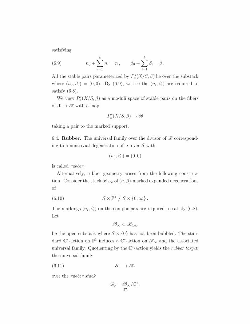
satisfying

(6.9) n0 +

k∑

i=1

ni = n , β0 +

k∑

i=1

βi = β .

All the stable pairs parameterized by P ⋆n(X/S, β) lie over the substack

where (n0, β0) = (0, 0). By (6.9), we see the (ni, βi) are required to

satisfy (6.8).

We view P ⋆n(X/S, β) as a moduli space of stable pairs on the fibers

of X → B with a map

P ⋆n(X/S, β) → B

taking a pair to the marked support.

6.4. Rubber. The universal family over the divisor of B correspond-

ing to a nontrivial degeneration of X over S with

(n0, β0) = (0, 0)

is called rubber.

Alternatively, rubber geometry arises from the following construc-

tion. Consider the stack B0,∞ of (n, β)-marked expanded degenerations

of

(6.10) S × P1/S × 0,∞ .

The markings (ni, βi) on the components are required to satisfy (6.8).

Let

B∞ ⊂ B0,∞

be the open substack where S × 0 has not been bubbled. The stan-

dard C∗-action on P1 induces a C∗-action on B∞ and the associated

universal family. Quotienting by the C∗-action yields the rubber target:

the universal family

(6.11) S −→ Br

over the rubber stack

Br = B∞/C∗ .

57

The universal family S carries the canonical divisors

S0 × Br , S∞ × Br ⊂ S .

Gluing S0 of the rubber target to the central fiber S of X embeds the

rubber stack into the stack of (n, β)-marked expanded degenerations

of X . We obtain the commutative diagram

(6.12) S

//

X

Br

// B .

Let R(n, β) denote the moduli space of stable pairs on the fibers of

(6.11). Concretely, R(n, β) is the moduli space of relative stable pairs

on

S × P1/S × 0,∞

with Euler characteristic n, class β, and no bubbling over S×0 – all

modulo the action of C∗. The compactness of R(n, β) is a consequence

of the C∗-quotient geometry.

We have seen that relative stable pairs on X/S near 0 ∈ ∆ are in fact

supported on the rubber target (6.12). Pushing forward from rubber

to the expanded degenerations of X/S yields a morphism

(6.13) ι : R(n, β) → P ⋆n(X/S, β)

which is a closed embedding of Deligne-Mumford stacks and a bijection

on closed points. The equation which cuts out R(n, β) ⊂ P ⋆n(X/S, β)

is the smoothing parameter of the first bubble.

We will prove ι is almost an isomorphism: ι satisfies the curvilinear

lifting property. To prove ι is an isomorphism, the smoothing param-

eter of the first bubble must be shown to vanish in all flat families

associated to the moduli space P ⋆n(X/S, β). We leave the isomorphism

question open.

6.5. Deformation theory. Following Section 6.1, let

ǫ : X → (∆, 0)58

be a K3-fibration for which α is m-rigid. Let β ∈ Eff(mα). We study

here the deformation theory of

P = P ⋆n(X/S, β) −→ B ,

the moduli space of stable pairs on the fibers of the right hand side of

the diagram (6.12). Identical arguments apply to the left hand side of

(6.12), replacing B by the substack Br and P by R(n, β) to give the

deformation theory of stable pairs on the rubber target.

Over X ×B P there is a universal stable pair

I• = OX×BPs−→ F ,

where the complex I• has O in degree 0. Let πP denote the projection

X ×B P → P and33

(6.14) E• = (RHomπP (I•, I•)0[1])

∨.

By [19, 34], P → B admits a relative perfect obstruction theory

(6.15) E• −→ LP/B

described as follows. Under the map LX×BP → L(X×BP )/B, the Atiyah

class At(I•) of I• projects to the relative Atiyah class:

(6.16)

Ext1(I•, I• ⊗ LX×BP

)// Ext1

(I•, I• ⊗

(LX/B ⊕ LP/B

)),

At(I•) // (AtX/B(I•),AtP/B(I•)) .

The map (6.15) is given by the partial Atiyah class AtP/B(I•) via the

following identifications:

Ext1(I•, I• ⊗ π∗PLP/B) = H1

(RHom(I•, I•)⊗ π∗

PLP/B)

= H0(RπP∗RHom(I•, I•)[1]⊗ LP/B

)

−→ H0(RπP∗RHom(I•, I•)0[1]⊗ LP/B

)

= Hom(E•,LP/B

).(6.17)

33Here RHomπP= RπP∗RHom is the right derived functor of

HomπP= πP∗Hom .

59

Defining E• to be the cone on the induced map E•[−1] → LB, we

obtain a commutative diagram of exact triangles:

(6.18) E• //

E• //

LB[1]

LP // LP/B // LB[1] .

The Artin stack B is smooth with LB a 2-term complex of bundles

supported in degrees 0 and 1. The induced map

ΩP = h0(E•) −→ h1(LB)

is onto because the points of P all have finite stabilizers by condition

(iv) above. Therefore the long exact sequence of sheaf cohomologies

of the top row of (6.18) shows E• has cohomology in degrees −1 and

0 only. The complex E• is perfect because E• and LB are. Since the

Deligne-Mumford stack P is projective, E• is quasi-isomorphic to a

2-term complex of locally free sheaves on P . Finally, the 5-Lemma

applied to the long exact sequences in cohomology of (6.18) implies

(6.19) E• −→ LP

is an isomorphism on h0 and onto on h−1. Therefore (6.19) is a perfect

obstruction theory for P .

The virtual dimension of Pn(X/S, β) is 0. The open and closed

component P ⋆n(X/S, β) ⊂ Pn(X/S, β) hence carries a virtual class of

dimension 0. We define

P ⋆n,β(X/S) =

∫

[P ⋆n(X/S,β)]

vir

1 .

Lemma 2. We have P ⋆n,β(X) = P ⋆

n,β(X/S).

Proof. Consider the degeneration of the total space X to the normal

cone of the special fiber S = ǫ−1(0). By the degeneration formula for

stable pairs invariants, P ⋆n,β(X) is expressed as a product of integrals

over P ⋆n1(X/S, β1) and Pn2(S × P1/S × 0, β2) where

n = n1 + n2 , β = β1 + β2 .60

Since the virtual class of Pn2(S ×P1/S ×0, β2) vanishes by the exis-

tence of the reduced theory (see Section 6.6 below), the only surviving

term of the degeneration formula is n1 = n and β1 = β.

6.6. Reduced obstruction theory. Let R = R(n, β) be the moduli

space of stable pairs on the rubber target.

The construction of the obstruction theory in Section 6.5 applies to

S ×Br R with the associated universal complex I• and projection πR to

R. The result is a relative obstruction theory for R given by a similar

formula:

(6.20) F • = (RHomπR(I•, I•)0[1])

∨ −→ LR/Br ,

and an absolute obstruction theory

(6.21) F • = Cone(F •[−1] −→ LBr

).

The relative obstruction sheaf of (6.20) contains H0,2(S) which can be

thought of as the topological or Hodge theoretic part of the obstruction

to deforming a stable pair. So long as S remains fixed, H0,2(S) is trivial

and can be removed. After removal, we obtain the reduced obstruction

theory . By now, there are many approaches to the reduced theory: see

[28] for an extensive account and references. We include here a brief

treatment.

We fix a holomorphic symplectic form σ on S. Let the 2-form σ

denote the pull-back of σ to S. The semiregularity map from the

relative obstruction sheaf ObF = h1((F •)∨) to OR plays a central role:

E xt2πR(I•, I•)0

∪At(I•)−→ E xt3πR(I•, I• ⊗ L(S×BrR)/Br )

−→ E xt3πR(I•, I• ⊗ ΩS/Br)

∧σ−→ E xt3πR(I•, I• ⊗ Ω3

S/Br)

tr−→ R3πR∗(Ω3S/Br

) −→ R3πR∗(ωS/Br)∼= OR .(6.22)

In the last line, ωS/Br is the fiberwise canonical sheaf. Using the simple

structure of the singularities, we see ωS/Br is the sheaf of fiberwise 3-

forms with logarithmic poles along the singular divisors in each fiber

with opposite residues along each branch. The canonical sheaf ωS/Br

inherits a natural map from Ω3S/Br

.61

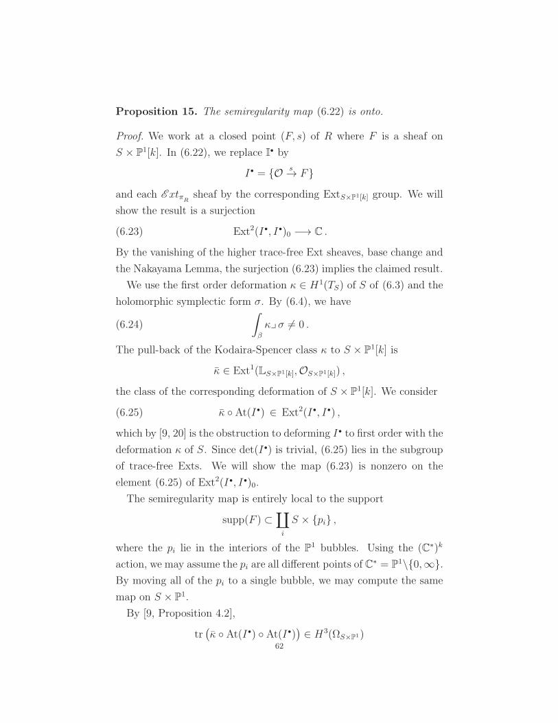
Proposition 15. The semiregularity map (6.22) is onto.

Proof. We work at a closed point (F, s) of R where F is a sheaf on

S × P1[k]. In (6.22), we replace I• by

I• = O s→ Fand each E xtπR sheaf by the corresponding ExtS×P1[k] group. We will

show the result is a surjection

(6.23) Ext2(I•, I•)0 −→ C .

By the vanishing of the higher trace-free Ext sheaves, base change and

the Nakayama Lemma, the surjection (6.23) implies the claimed result.

We use the first order deformation κ ∈ H1(TS) of S of (6.3) and the

holomorphic symplectic form σ. By (6.4), we have

(6.24)

∫

β

κy σ 6= 0 .

The pull-back of the Kodaira-Spencer class κ to S × P1[k] is

κ ∈ Ext1(LS×P1[k],OS×P1[k]) ,

the class of the corresponding deformation of S × P1[k]. We consider

(6.25) κ At(I•) ∈ Ext2(I•, I•) ,

which by [9, 20] is the obstruction to deforming I• to first order with the

deformation κ of S. Since det(I•) is trivial, (6.25) lies in the subgroup

of trace-free Exts. We will show the map (6.23) is nonzero on the

element (6.25) of Ext2(I•, I•)0.

The semiregularity map is entirely local to the support

supp(F ) ⊂∐

i

S × pi ,

where the pi lie in the interiors of the P1 bubbles. Using the (C∗)k

action, we may assume the pi are all different points of C∗ = P1\0,∞.By moving all of the pi to a single bubble, we may compute the same

map on S × P1.

By [9, Proposition 4.2],

tr(κ At(I•) At(I•)

)∈ H3(ΩS×P1)

62

equals 2κy ch2(I•). Therefore, the image of κ At(I•) under the map

(6.23) is

(6.26) 2

∫

S×P1

(κy ch2(I•)) ∧ σ = −2

∫

S×P1

(κy σ) ∧ ch2(I•) ,

by the homotopy formula

(6.27) 0 = κy (ch2(I•) ∧ σ) = (κy ch2(I

•)) ∧ σ + (κy σ) ∧ ch2(I•) .

Since ch2(I•) is Poincare dual to −β, we conclude (6.26) equals

2

∫

β

κy σ ,

which is nonzero (6.24) by the choice of κ.

Composing (6.22) with the truncation map (F •)∨ → h1((F •)∨)[−1]

and dualizing gives a map

(6.28) OR[1] −→ F • .

Proposition 16. The map (6.28) lifts uniquely to the absolute obstruc-

tion theory F • of (6.21).

Proof. To obtain a lifting, we must show the composition

OR[1] −→ F • −→ LR/Br −→ LBr [1]

is zero. In fact, the composition of the second and third arrows is

already zero on R. We will show the vanishing of the dual composition

(6.29) (LBr)∨[−1] −→ (LR/Br)

∨ −→ (F •)∨ .

We work with the universal complex I• on S ×Br R. By (6.16), we

have the diagram (in which we have suppressed some pull-back maps):

L∨Br[−1] // L∨

S/Br⊕ L∨

R/Br//

AtS/Br (I•)⊕ AtR/Br (I

•)

L∨S×BrR

At(I•)

RHom(I•, I•)0[1] RHom(I•, I•)0[1] .

The top row is an exact triangle, so the induced map

L∨Br[−1] −→ RHom(I•, I•)0[1]

63

vanishes.34 Therefore the composition

(6.30) π∗RL

∨Br[−1] // π∗

SL∨S/Br

AtS/Br (I•)

// RHom(I•, I•)0[1]

equals minus the composition

(6.31) π∗RL

∨Br[−1] // π∗

RL∨R/Br

AtR/Br (I•)

// RHom(I•, I•)0[1] .

By adjunction the composition (6.31) gives the composition

(6.32) L∨Br[−1] // L∨

R/Br

AtR/Br (I•)

// RπR∗RHom(I•, I•)0[1] ,

which by (6.15, 6.17, 6.20) is precisely the composition (6.29) we want

to show is zero. So it is sufficient to show (6.30) vanishes.

The first arrow of (6.30) is (the pull-back from Br to R of) the

Kodaira-Spencer class of S/Br: the final arrow in the exact triangle

LBr −→ LS −→ LS/Br −→ LBr [1] .

Away from the singularities S × 0,∞ in each S × P1-bubble, S is

locally a trivial family over Br: it is isomorphic to

S × C∗ × Br

locally35 over Br. Therefore this Kodaira-Spencer map vanishes in a

neighborhood of the support of the universal sheaf F. But the second

arrow of (6.30) – the Atiyah class AtS/Br(I•) of I• – is nonzero only on

the support of F, so the composition is zero.

Finally, choices of lift are parameterized by Hom(OR[1],LBr). This

vanishes because LBr is concentrated in degrees 0 and 1. Therefore the

lift is unique.

The relative and absolute reduced obstruction theories are defined

respectively by:

(6.33)

F •

red = Cone(OR[1] −→ F •

), F •

red = Cone(OR[1] −→ F •

)

34There is no obstruction to deforming as we move through R over the base Br:there indeed exists a complex I• over all of S ×Br

R.35But not globally due to the nontrivial C∗-action on the C factor giving a

nontrivial line bundle over Br.64

The associated obstruction sheaves

ObredF = h1((F •

red)∨) , Obred

F = h1((F •

red)∨)

are the kernels of the induced semiregularity maps

(6.34) ObF −→ OR , ObF −→ OR ,

with the first given by (6.22).

Though not required here, one can show [28, 41] the complexes (6.33)

do indeed define perfect obstruction theories for R. For our purposes

of extracting invariants, the simpler cosection method of Kiem-Li [25]

is sufficient to produce the reduced virtual cycle [R]red as in [36].

We summarize here the cosection method for the reader. Writing

(F •)∨ = F0 −→ F1

as a global two-term complex of locally free sheaves on R, Behrend and

Fantechi [3] produce a cone

C ⊂ F1 such that [R]vir = 0!F1C = [s(C)c(F1)]virdim .

Here, s is the Segre class, c is the total Chern class, and we take the

piece in degree equal to the virtual dimension

virdim = rankF0 − rankF1 .

Kiem and Li show the cone C lies cycle theoretically (rather than

scheme theoretically) in the kernel K of the composition

F1 −→ Ob −→ OR.

We define the reduced virtual cycle in the reduced virtual dimension

(virdim + 1) by

(6.35) [R]red = 0!KC = [s(C)c(K)]virdim+1 .

The reduced class is much more interesting than the standard virtual

class from the point of view of invariants: the exact sequence

0 −→ K −→ F1 −→ OR −→ 065

implies the vanishing of the standard virtual class,36

[R]vir = c1(OR).[R]red + [s(C)c(K)]virdim = 0 .

(The second term vanishes because C is a cycle inside K, so s(C)c(K)

is a sum of cycles in dimension ≥ rankF0 − rankK = virdim + 1.)

The vanishing reflects the fact that we can deform S along κS (6.24):

β does not remain of type (1, 1) so there can be no holomorphic curves

in class β.

We define the reduced rubber invariants of S via integration over the

dimension 0 class (6.35):

(6.36) Rredn,β(S ×R) =

∫

[R(n,β)]red1 .

Here R denotes the rubber, the quotient by C∗ of the relative geometry

P1/0,∞.

6.7. Comparison of obstruction theories. We have constructed

three obstruction theories:

(i) F • on the rubber moduli space R,

(ii) F •

red on the rubber moduli space R,

(iii) E• on the moduli space P ⋆ of stable pairs on X/S over 0 ∈ ∆.

Our goal in Sections 6.7 - 6.9 is to relate (i), (ii), and (iii).

By pushing stable pairs forward from the rubber to the expanded

degenerations of X/S, we get a map (6.13):

ι : R −→ P ⋆.

Since E• and F • were defined by essentially the same formulas (6.14)

and (6.20) respectively, we see

(6.37) ι∗E• ∼= F •.

36In our particular situation, the vanishing is even more obvious since the stan-dard virtual dimension is −1. Since the reduced virtual dimension is 0, the reducedvirtual class is nonetheless nontrivial in general.

66

The definitions of E• and F • (6.18 and 6.21) then yield the following

diagram of exact triangles on R:

(6.38) N∗

N∗

ι∗LB//

ι∗E• //

ι∗E•

LBr// F • // F • ,

where N∗ = LBr/B[−1] is the conormal bundle of the divisor Br ⊂ B.

Dualizing the central column and passing to cohomology gives a map

(6.39) N −→ ObF = h1((F •)∨)

which describes the obstruction to deforming a pair in the image of ι

off the rubber and into the bulk of X/S. Composing with the semireg-

ularity map (6.34) gives

(6.40) N −→ OR .

The rest of Section 6.7 will be devoted to proving the following result.

Proposition 17. The maps (6.39, 6.40) are injections of sheaves on

R. Moreover, (6.39) has no zeros.

Connected case. We first work at a stable pair (F, s) with connected

support. The sheaf F is therefore supported on S × (P1\0,∞) withno further bubbles in the rubber.37 We will show that the composition

(6.40) is an isomorphism at the point (F, s). By the vanishing of the

higher trace-free Exts, base change and the Nakayama Lemma, the

Proposition will follow in the connected support case.

A chart for the stack B of (n, β)-marked expanded degenerations of

X/S in a neighborhood of the 1-bubble locus is C/C∗ with universal

family X → B given by [32]

(6.41) BlS×0(X × C)

x C∗

C x C∗.

37If we view the stable pair as lying in X/S, there is a single bubble and (F, s)is supported in its interior.

67

Here, the trivial C∗-action on X and the usual weight 1 action on C

yield a C∗-action on X×C. The blow up along the C∗-fixed subvariety

S × 0 has a canonically induced C∗-action. The exceptional divisor

S × P1 inherits a C∗-action. The central fiber is

X [1] = X ∪S (S × P1) .

More explicitly, let x denote the coordinate on X pulled back locally

at 0 ∈ ∆ from the base of the K3-fibration

(6.42) X → ∆ ,

and let t denote the coordinate pulled back from the C-base of (6.41).

By definition,

(6.43) BlS×0(X × Ct) ist = λx

⊂ X × Ct × P1

λ ,

where x has C∗-weight 0 while t and λ have weight −1. Here, λ is the

usual coordinate on P1 which takes the value ∞ on the relative divisor

S × ∞ in the central fiber, and the value 0 on the proper transform

X × 0 of the central fiber. Removing these loci, which are disjoint

from the support of (F, s), our universal family over B becomes the

quotient by C∗ of

(6.44) X × C∗λ

t=λx// Ct .

The key to Proposition 17 is the following observation: as we move in

the direction ∂t in the base of (6.44), we move away from the central

fiber S ⊂ X in the direction λ−1∂x over the base of the K3-fibration

(6.42). In other words, on the central fiber S×C∗λ, the Kodaira-Spencer

class of the family (6.44) applied to ∂t is

(6.45) λ−1κ ∈ Γ(OC∗)⊗H1(TS) ∼= H1(TX |S×C∗) .

Here, as usual, κ ∈ H1(TS) is the Kodaira-Spencer class (6.3) of (6.42)

on the central fiber S. Since λ 6= ∞ on the support of (F, s), the (0, 2)-

part of the class β of F immediately becomes nonzero along λ−1∂x,

just as in the proof of Proposition 15. Thus the semiregularity map is

nonzero. We now make the argument more precise.68

The semiregularity map (6.34) of Proposition 16 was first defined on

F •. After rearranging (6.38), we see the composition (6.40) we require

is induced from the composition

(6.46) ι∗L∨B−→ (ι∗E•)∨[1] ∼= (F •)∨[1] −→ OR .

The last arrow is (6.28). By (6.38), the first arrow is zero on composi-

tion with L∨Br

→ ι∗L∨B, so the first arrow factors through the cone N

as required. In fact, we even have a splitting

(6.47) ι∗L∨B

∼= N ⊕ L∨Br,

obtained from expressing B locally as C/C∗, with the substack Br

given by 0/C∗. Therefore,

LB∼= ΩC → g∗ ⊗OB ,

where g is the Lie algebra of C∗, and, in the standard trivialization, the

map takes dt to t. On applying ι∗ the map therefore vanishes, leaving

ι∗ΩC ⊕ (g∗ ⊗OBr)[−1] = N∗ ⊕ LBr

as claimed.

By the same argument as in (6.30–6.32), the first arrow of (6.46) is

(up to a sign) the composition of the following Kodaira-Spencer and

Atiyah classes:

ι∗L∨B

// RπR∗(ι∗L∨

X/B)[1]AtX/B(I•)

// RπR∗RHom(I•, I•)0[2] .

Together with the splitting (6.47) and the description (6.46) of our

map, we find that at a point I• the map (6.40) is the composition

(6.48) N |I• −→ Ext1(LX[1],OX[1]) −→ Ext2(I•, I•)0 −→ C .

The first arrow is the Kodaira-Spencer class of the family (6.41) on the

central fiber X [1]. The connected support of our stable pair (F, s) is

contained in S × 1, without loss of generality. On restriction to this

support, the Kodaira-Spencer class is κ (6.44, 6.45).38

38If we act by λ ∈ C∗ the relevant statement becomes that for a stable pairsupported in S ×λ, the value of the Kodaira-Spencer class on λ∂t is λ.λ

−1κ = κ(6.45). The point is that there is no natural trivialisation of N , and λ ∈ C∗ takesthe trivialization ∂t to the trivialization λ∂t.

69

The second arrow is composition with the Atiyah class of the complex

I• onX [1]. The Atiyah class vanishes on the complement of the support

S ×1. We may restrict I• to the bubble S × P1λ and calculate there.

The final arrow is the semiregularity map (6.22). So (6.48) simplifies

to the composition

(6.49) Cκ

// H1(TS×P1)At(I•)

// Ext2S×P1(I•, I•)0tr( · At(I•)∧σ)

// C ,

where again we have trivialized N by the section ∂t. The composition

is therefore ∫

S×P1

tr(κ At(I•) At(I•)) ∧ σ .

By [9, Proposition 4.2], this is

2

∫

S×P1

κy ch2(I•) ∧ σ = −2

∫

S×P1

(κy σ) ∧ ch2(I•) = 2

∫

β

κy σ ,

just as in (6.26). Since κy σ is nonzero on β by design (6.4), the compo-

sition (6.49) is nonzero. Proposition 17 is established in the connected

case.

Disconnected case. To deal with the case of arbitrary support, we

write a stable pair (F, s) on the rubber target as a direct sum of stable

pairs with connected supports:

(6.50) (F, s) =⊕

i

(Fi, si) .

By stability we may assume, without loss of generality, that (F1, s1) is

supported on the interior of the first bubble.

The decomposition (6.50) holds in a neighborhood of (F, s) in the

moduli space R (though the ith summand need not have connected

support for pairs not equal to (F, s)). The obstruction sheaf ObF is

additive with respect to the decomposition: E xt2πR(I•, I•)0 splits into a

corresponding direct sum. We will prove (6.40) is an isomorphism on

the summand (F1, s1). The isomorphism will follow from the connected

case after we have set up appropriate notation. Since the map (6.39)

is linear, the result will prove (6.39) has no zeros. We will address the70

injectivity claim for the map (6.40) in the statement of Proposition 17

at the end of the proof.

Suppose (F, s) is supported on X [k]. In a neighborhood of X [k], a

chart for the stack of (n, β)-marked expanded degenerations of X is

given by

(6.51) Ck/(C∗)k

where the group acts diagonally [32]. We let t1, . . . , tn denote the coor-

dinates on the base Ck. Let x be the coordinate pulled back from the

base ∆ of the K3-fibration X .

The universal family

(6.52) X → B ,

restricted to the chart (6.51), is constructed by the following sequence

of (C∗)k-equivariant blow-ups of X × Ck:

• Blow-up X × Ck along x = 0 = t1 (the product of the surface

S ⊂ X and the first coordinate hyperplane).

• Blow-up the result along the proper transform of x = 0 = t2,

(the proper transform of S times the second coordinate hyper-

plane).

• At the ith stage, blow-up the result of the previous step in the

proper transform of x = 0 = ti.

After k steps, we obtain the universal family (6.52) over the chart

(6.51).

The fiber of the universal family over the origin of (6.51) is X [k]

with marking

(n0, β0) ∈ Z⊕H2(X,Z)

on the first component and marking (ni, βi) ∈ Z⊕H2(S,Z) on the ith

bubble for 1 ≤ i ≤ k. The data satisfy (6.9):

n0 +k∑

i=1

ni = n , β0 +k∑

i=1

βi = β .

71

Over a point of Ck with precisely j of the coordinates ti vanishing,

the fiber is X [j]. The j vanishing coordinates are in bijective ordered

correspondence with the j bubbles and the j creases39 of X [j]. Moving

away from this point of the base, a crease smooths if and only if the

corresponding coordinate becomes nonzero. If the ith and (i + 1)th

vanishing coordinates are ta and tb, then the marking on the ith bubble

of X [j] is (b−1∑

i=a

ni ,

b−1∑

i=a

βi

)∈ Z⊕H2(S) .

Similarly, if the first vanishing coordinate is tc, then the marking on

X ⊂ X [j] is

(6.53)

(n0 +

tc−1∑

i=1

ni , β0 +

tc−1∑

i=a

βi

)∈ Z⊕H2(X) .

Relative stable pairs – which cannot lie in X – all lie over the locus

t1 = 0, n0 = 0, β0 = 0 ,

where c = 1 in (6.53) and the marking on X vanishes. The inclusion

of the hyperplane t1 = 0,

(6.54) ι : Ck−1/(C∗)k = t1 = 0

/(C∗)k −→ Ck

/(C∗)k

describes the inclusion (6.12) of the corresponding chart of the stack

Br ⊂ B over which the rubber target S lies.

On the chart (6.51),

LB =ΩCk −→ (g∗)k ⊗OB

,

where the map is diag (t1, . . . , tk) in the natural trivializations. Pulling

back by (6.54) gives

ι∗LB =(N∗ ⊕ g∗ ⊗OBr [1]

)⊕ΩCk−1

diag(t2,...,tk)// (g∗)k−1 ⊗OBr

= N∗ ⊕ LBr .

39The ith crease of X [j] is the copy of S at the bottom of the ith bubble: theintersection of the (i− 1)th and ith bubbles of X [j].

72

Thus ι∗L∨B

∼= N ⊕ L∨Br

just as in (6.47). The element ∂t1 lies in –

and generates – the first summand (but, just as before, is not a global

trivialisation as it is not C∗-invariant).

We have to work out the composition (6.48) as before, replacing ∂t

by ∂t1 . The stable pair (F1, s1) is supported on some S × 1 of the

first bubble of X [k] just as before. Restricting to the first bubble,

the Kodaira-Spencer class evaluated on the section ∂t1 of N is κ just

as in the single bubble case: all further blow-ups in the construction

of X → B occur at S × ∞ in the bubble and hence do not affect

the interior of the first bubble or its Kodaira-Spencer class. The same

calculation then shows the map (6.40) at the point (F1, s1) takes ∂t1 to

(6.55) 2

∫

β1

κy σ ,

where β1 = [F1]. Since (6.55) is nonzero by (6.4), the map (6.40) is an

isomorphism on the first summand (F1, s1) as claimed. As explained

above, this implies that (6.39) has no zeros.

Consider now the summand (F2, s2). If the support of (F2, s2) is

in the first bubble, the support lies in S × λ for some λ 6= 1, and

the work we have already done shows that applied to (F2, s2) the map

(6.40) takes ∂t1 to

(6.56) 2λ−1

∫

β2

κy σ 6= 0 .

Here, the nonvanishing is by (6.4) applied to β2 = [F2].

For summands (Fi, si) not in the first bubble we can do a similar

calculation, blowing up (6.43) once more and using local coordinates

again. The result is that the Kodaira-Spencer class in the higher bub-

bles is 0 (this is effectively the λ→ ∞ limit of the above calculation).

To prove the injectivity claim for the map (6.40) in the statement of

Proposition 17, we consider two possibilitites.

• If (F1, s1) is the only summand in the first bubble, all others

contribute zero to (6.40), so in total (6.40) is nonzero by (6.55).73

• If there is another summand (F2, s2) in the first bubble, then,

by linearity, the nonzero contribution (6.56) of (F2, s2) is added

to that of the other summands, and can be varied by perturbing

its support

λ ∈ C∗ ⊂ P1 .

Therefore, even though the map (6.40) might be zero at (F, s),

the map (6.40) is nonzero at a nearby perturbation. Since the

perturbation by moving the support λ is along an etale trivial

factor in the moduli space R, the map (6.40) must be injective

as a morphism of sheaves.

The proof of Proposition 17 is complete.

6.8. Curvilinear lifting. Proposition 17 does not imply the moduli

spaces R and P ⋆ are isomorphic. Our analysis of Rn,β is crucially

dependent upon a weaker curvilinear lifting relationship between R

and P ⋆ which does follow from Proposition 17.

Lemma 3. The map ι : R → P ⋆ of (6.13) induces an isomorphism

ι∗ΩP ⋆ ∼= ΩR of cotangent sheaves.

Proof. The obstruction theories E•, F • are related by the exact triangle

N∗ −→ ι∗E• −→ F •

of (6.38), giving the exact sequence

h−1(F •) −→ N∗ −→ h0(ι∗E•) −→ h0(F •) −→ 0 .

Since E• vanishes in strictly positive degrees and ι∗ is right exact,

h0(ι∗E•) = ι∗h0(E•). Therefore, we obtain

(6.57) h−1(F •) −→ N∗ −→ ι∗ΩP ⋆ −→ ΩR −→ 0 .

By Proposition 17, the first map is surjective.

Corollary 2. Suppose A is a subscheme of B with ideal J satisfying

(6.58) d : J → ΩB|A injective.

(In particular J2 = 0.) Then any extension f : B → P ⋆ of a map

f : A→ R factors through R.74

Proof. Let I denote the ideal of R inside P . To show the factorization

of f through R, we must show the image of

f ∗I → J

vanishes. Since J2 = 0, the above image can be evaluated after restric-

tion to A,

(6.59) f ∗I|A = f ∗I → J .

By Lemma 3, the first map d vanishes in the exact sequence of Kahler

differentials

Id−→ ι∗ΩP ⋆ −→ ΩR −→ 0 .

Pulling-back via f gives the top row of the following commutative di-

agram with exact rows.

f ∗I

f∗

0// f ∗ι∗ΩP ⋆

f∗

∼// f ∗ΩR

f∗

// 0

0 // Jd

// ΩB|A // ΩA // 0 .

Here, the central map uses the isomorphism f ∗ι∗ΩP ⋆ ∼= (f ∗ΩP ⋆)|A. Asa result, the first vertical arrow (given by (6.59)) is zero. Hence, f has

image in R.

The basic relationship between R and P ⋆ which we need is the curvi-

linear lifting property proven in the following Corollary.

Corollary 3. Every map SpecC[x]/(xk) → P ⋆ factors through R.

Proof. Since R ⊂ P ⋆ is a bijection of sets, we have the result for k = 1.

Since

A = SpecC[x]

(xk)⊂ Spec

C[x]

(xk+1)= B

satisfies (6.58), the result for higher k follows by Corollary 2 and in-

duction.

We summarize the above results in the following Proposition.

Proposition 18. The map ι : R → P ⋆ of (6.13) is a closed embed-

ding of Deligne-Mumford stacks which satisfies the curvilinear lifting

property.

75

The complexes ι∗E•, F •, and F •

red on R are related by the exact

triangles

(6.60) (F •

red)∨

(F •

red)∨

N [−1] // (F •)∨ //

(ι∗E•)∨

N [−1] // OR[−1] // OD[−1] .

Here, D is the Cartier divisor on which the injection N → OR (6.40)

vanishes.

In particular, in K-theory the classes of (ι∗E•)∨ and (F •

red)∨ differ

by OD[−1]. The K-theory classes determine the corresponding virtual

cycles via the formula of [15, 43]. For the virtual class [P ⋆]vir associated

to E•, the formula is

(6.61) [P ⋆]vir =[s((E•)∨

)∩ cF (P ⋆)

]virdim

,

where cF (P⋆) is the Fulton total Chern class [15, 4.2.6.(a)] of the scheme

P ⋆, s denotes the total Segre class, and the subscript denotes the term

in degree specified by the virtual dimension (equal to 0 here). The

homology class cF (P⋆) is not of pure degree. The expression (6.61) is a

sum of different degree parts of the cohomology class s((E•)∨

)capped

with the different degree parts of cF (P⋆) to give the virtual class.

Since the reduced scheme structure of R and P ⋆ is the same, we

may view cF (P⋆) and [P ⋆]vir as cycles on R. The curvilinear lifting

property of Proposition 18 implies a basic relation between the Fulton

Chern classes of R and P ⋆ explained in Appendix C.2,

(6.62) cF (R) = cF (P⋆) ∈ A∗(R) .

Formulas (6.61) and (6.62) allow us to study [P ⋆]vir via the geometry

of R.

Since s(OD) = 1 − D, the rightmost column of (6.60) yields the

identity

s((ι∗E•)∨

)= s

((F •

red)∨)+D. s

((ι∗E•)∨

).

76

After substituting in (6.61), we obtain

[P ⋆]vir =[s((F •

red)∨)∩ cF (P ⋆)

]0+[s((ι∗E•|D)∨

)∩ cF (P ⋆)|D

]0

=[s((F •

red)∨)∩ cF (R)

]0+[s((ι∗E•|D)∨

)∩ cF (R)|D

]0

(6.63)

= [R]red +[s((ι∗E•|D)∨

)∩ cF (R)|D

]0.

We may replace D in the rightmost term by any other Cartier divisor

in the same linear equivalence class, since the replacement leaves the

K-theory class [OD] unchanged. We will work on a cover of the rubber

moduli space R on which D becomes linearly equivalent to a rather

more tractable divisor.

6.9. Rigidification. Let R = R(n, β) be the moduli space of stable

pairs on the rubber target. Let

(6.64) π : U(n, β) = S ×Br R→ R

be the universal target over the rubber moduli space R. Let

(6.65) W (n, β) ⊂ U(n, β)

denote the open set on which the morphism π is smooth.

We view U as a moduli of pairs (r, p) where r ∈ R and p is a point

in the rubber target associated to r. For pairs (r, p) ∈ W , the point p

is not permitted to lie on any creases. Hence, the restriction

π : W → R

is a smooth morphism. The rubber target admits a natural map,

ρ :W → S ,

to the underlying K3 surface.

Viewing [R]red and [P ⋆]vir as cycle classes on R, we define classes

[W ]red and [W ]vir on W by flat pull-back:

[W ]red = π∗[R]red , [W ]vir = π∗[P ⋆]vir.

By the definitions of the cones and the Fulton class,

(6.66) [W ]red =[s((π∗F •

red)∨)s(Tπ)∩ cF (W )

]3,

77

where Tπ on W is the relative tangent bundle of π. Similarly,

(6.67) [W ]vir =[s((π∗ι∗E•)∨

)s(Tπ)∩ cF (W )

]3.

Integrals over R may be moved to W by the following procedure. To

a class δ ∈ H2(S,Q), we associate a primary insertion

T0(δ) = ch2(F) ∪ ρ∗(δ) ∈ H6(U,Q

),

where F is the universal sheaf. The key identity is the divisor formula

obtained by integrating down the fibers of (6.64):

(6.68) π∗(T0(δ)

)= 〈δ, β〉 =

∫

β

δ ∈ H0(R,Q) .

The push-forward π∗ is well-defined since ch2(F) and T0(δ) are sup-

ported on Supp(F) which is projective over R via π.

The derivation in Section 6.8 of (6.63) can be pulled-back via π to

W to yield:

(6.69) [W ]vir = [W ]red +[s((π∗ι∗E•|D)∨

)s(Tπ)∩ cF (W )|D

]3.

As before, D is any divisor representing the first Chern class of the

pull-back of N∗, the conormal bundle of the divisor Br ⊂ B. By

integration against (6.69), formula (6.68) yields

(6.70) P ⋆n,β(X)− Rred

n,β(S ×R) =

1

〈δ, β〉

∫

D

(s((π∗ι∗E•|D)∨

)s(Tπ)∩ cF (W )|D

)· T0(δ) .

We describe next a geometric representative for D.

Attaching the infinity section S∞ of the rubber over R(n1, β1) to the

zero section S0 of rubber over W defines a divisor

(6.71) Dn1,β1 = R(n1, β1)×W (n2, β2) ⊂ W (n, β) ,

whenever (n1, β1) + (n2, β2) = (n, β). The following result is a form of

topological recursion.

Lemma 4. The line bundle π∗N∗ has a section with zeros given by the

divisor

D =∑

n1,β1

Dn1,β1 .

78

The sum is over the finitely many (n1, β1) ∈ Z ⊕ H2(S,Z) for which

Dn1,β1 is nonempty.

Proof. The universal family X → B has smooth total space. Moving

normal to Br smooths the first crease in the expanded degeneration X :

the crease where X joins the rubber S across S ⊂ X and the 0-section

S0 of the rubber. Therefore the normal bundle N , pulled back to Xand restricted to the first crease, is isomorphic to

NS⊂X ⊗NS0⊂S .

Fixing once and for all a trivialization of NS⊂X , we find that

N ∼= ψ∗0

is isomorphic to the tangent line to P1 on the zero section.40

Now pull-back to W (n, β) via (6.64). By forgetting S (but remem-

bering the Z⊕H2(S,Z) marking), W (n, β) maps to the stack Bpn,β of

(n, β)-marked expanded degenerations of P1/0,∞,

(6.72) W (n, β) → Bpn,β .

The moduli space W (n, β) parameterizes pairs (r, p). The map (6.72)

is defined by using p to select the rigid component and to determine

1 ∈ P1. The cotangent line at the relative divisor 0 defines a line bundle

on Bpn,β which we also call ψ0. On W (n, β), ψ0 pulls-back to

π∗ψ0∼= π∗N∗

above.

Pick a nonzero element of T ∗P1|0, pull-back to any expanded degener-

ation, and restrict to the new 0-section. We have constructed a section

of ψ0 over Bpn,β which vanishes precisely on the divisor where 0 has

been bubbled. The latter divisor is the sum of the divisors Dn1,β1 as

required.

40More precisely, fix any point s ∈ S. Then the corresponding point of the zerosection S0 of S defines a section s0 of S → Br. The first bubble is S0 × P1, andthe conormal bundle to S0 is the restriction of T ∗

P1 ⊂ T ∗

S0×P1 . Pulling back by s0gives the cotangent line ψ0.

79

After combining Lemma 4 with (6.70), we obtain the formula:

(6.73) P ⋆n,β(X)− Rred

n,β(S ×R) =

1

〈δ, β〉∑

n1,β1

∫

Dn1,β1

(s((π∗ι∗E•)∨

)s(Tπ)|Dn1,β1

∩ cF (W )|Dn1,β1

)· T0(δ) .

To proceed, we must to compute the restriction of π∗ι∗E• to the divisor

Dn1,β1.

The relative obstruction theory is given by the same formula (6.15)

on the moduli spaces R and P ⋆. On R, the relative obstruction theory

was denoted F • (6.20). Since the relative obstruction theory is additive

over the connected components of a stable pair,

(6.74) π∗ι∗E•∣∣Dn1,β1

∼= ι∗E•

R(n1,β1)⊕ π∗F •

W (n2,β2),

where we have split Dn1,β1 as R(n1, β1)×W (n2, β2) using (6.71).

As in (6.18, 6.21) the relationship of the relative to the absolute

obstruction theories E•

W and F • is through the usual exact triangles:

(6.75) ι∗E• −→ ι∗E• −→ ι∗LBn,β[1]

on the moduli space R and

(6.76) ι∗E•

R(n1,β1)⊕ π∗F •

W (n2,β2)−→ ι∗E•

R(n1,β1)⊕ π∗F •

W (n2,β2)

−→ ι∗LBn1,β1[1]⊕ π∗LBr [1]

onDn1,β1 = R(n1, β1)×W (n2, β2). InK-theory, the isomorphism (6.74)

and the exact sequences (6.75)-(6.76) yield

(6.77)[π∗ι∗E•

∣∣Dn1,β1

]= [ι∗E•

R(n1,β1)] + [π∗F •

W (n2,β2)]

− [ι∗LBn1,β1]− [π∗LBr ] + [ι∗LBn,β

] .

Since Dn1,β1 is pulled-back41 from Bn,β, the standard divisor conor-

mal bundle sequence yields

[LBn1,β1] + [LBr ]− [LBn,β

] = −[ODn1,β1(−Dn1,β1)] .

41More precisely, Dn1,β1⊂W is an open and closed component of the pull-back.

80

Hence, we obtain

(6.78) s((π∗ι∗E•

∣∣Dβ1,n1

)∨)c(ODn1,β1

(Dn1,β1))

= s((ι∗E•

R(n1,β1))∨)s((π∗F •

W (n2,β2))∨)

By the basic properties of cones and the embeddingDn1,β1 ⊂W (n, β)

discussed in Appendix C.3, we have

(6.79) cF (W (n, β))∣∣Dn1,β1

= cF (Dn1,β1)c(ODn1,β1(Dn1,β1)) .

We replace cF (W (n, β))∣∣Dn1,β1

by (6.79) in (6.73). After using (6.78)

to cancel the c(ODn1,β1(Dn1,β1)) term, we obtain42

1

〈δ, β〉∑

n1,β1

∫

R(n1,β1)

s((ι∗E•)∨) ∩ cF (R(n1, β1))

×∫

W (n2,β2)

(s((π∗F •)∨)s

(Tπ)∩ cF (W (n2, β2))

)· T0(δ) .

Since the two obstruction theories F • and F •

red onW (n2, β2) differ only

by the trivial line bundle,

s((F •)∨) = s((F •

red)∨) .

By another application of the rigidification formula (6.68), we obtain

P ⋆n,β(X)−Rred

n,β(S×R) =1

〈δ, β〉∑

n1,β1

P ⋆n1,β1

(X) · 〈δ, β2〉Rredn2,β2

(S×R) .

6.10. Logarithm. Let α ∈ Pic(S) is a primitive class which is positive

with respect to a polarization, and let β ∈ Eff(mα). The only effective

decompositions of β are

β = β1 + β2 , βi ∈ Eff(mα) .

We formulate the last equation of Section 6.9 as the following result.

42The integration over W (n2, β2) is well-defined since the insertions τ0(δ) yieldsa complete cycle as before.

81

Theorem 5. For the family ǫ : X → (∆, 0) satisfying conditions

(i,ii,⋆) of Section 6.1 for mα, we have

P ⋆n,β(X)− Rred

n,β(S ×R) =

1

〈δ, β〉∑

n1+n2=n

∑

β1+β2=β

P ⋆n1,β1

(X) · 〈δ, β2〉Rredn2,β2

(S ×R)

for every β ∈ Eff(mα) and δ ∈ H2(S,Z) satisfying 〈δ, β〉 6= 0.

The basic relationship between P ⋆n,β(X) and Rred

n,β(S × R) is an im-

mediate Corollary of Theorem 5. Let

P ⋆β (X) =

∑

n∈Z

P ⋆n,β(X) qn , Rred

β (S ×R) =∑

n∈Z

Rredn,β(S ×R) qn .

Corollary 4. For β ∈ Eff(mα),

P ⋆β (X) = Coeffvβ

exp

∑

β∈Eff(mα)

vβRredβ

(S ×R)

.

Proof. Since δ ∈ H2(S,Z) is arbitrary, Theorem 5 uniquely determines

P ⋆β (X) in terms of Rred

βi(S × R) for βi ∈ Eff(mα). We see Corollary

4 implies exactly the recursion of Theorem 5 by differentiating the

exponential. To write the differentiation explicitly, let

v1, . . . , v22 ∈ H2(S,Z)

be a basis. For β =∑22

i=1 bivi, we write

vβ =

22∏

i=1

vbii .

Let 〈δ, vi〉 = ci. Then, differentiation of the equation of Corollary 4 by

22∑

i=1

civi∂

∂vi

yields the recursion of Theorem 5.

82

6.11. Definition of Rn,β. We now return to the definition of stable

pairs invariants for K3 surface given in Section 6.2.

Let α ∈ Pic(S) be a primitive class which is positive with respect to

a polarization. Let

ǫ : X → (∆, 0)

satisfying the conditions of Section 6.1: (i), (ii), and (⋆) for mα. We

have

Rmα(S) = Coeffvmα

log

1 +

∑

β∈Eff(mα)

vβP ⋆β (X)

.

Let Rn,mα(S) be the associated q coefficients:

Rmα(S) =∑

n∈Z

Rn,mα(S) qn .

By Corollary 4 of Theorem 5, we can take the logarithm.

Proposition 19. We have Rmα(S) = Rredmα(S ×R).

Proof. By Corollary 4 and the above definition,

Rmα(S) = Coeffvmα

log exp

∑

β∈Eff(mα)

vβRredβ

(S ×R)

= Coeffvmα

∑

β∈Eff(mα)

vβRredβ

(S ×R)

.

Hence, if mα ∈ Pic(S) is effective, Rmα(S) = Rredmα(S × R). If mα ∈

Pic(S) is not effective, both Rmα(S) and Rredmα(S ×R) vanish.

Proposition 19 is the main point of Section 6. The complete geo-

metric interpretation of the logarithm as integration over a moduli of

stable pairs is crucial for our proof of the KKV conjecture.

6.12. Dependence. Let α ∈ Pic(S) be a primitive class which is pos-

itive with respect to a polarization. As a consequence of Proposition

19, we obtain a dependence result.83

Proposition 20. Rmα(S) depends only upon m and

〈α, α〉 = 2h− 2

and not upon S or the family ǫ.

From the definition of Rmα(S), the dependence statement is not im-

mediate (since the argument of the logarithm depends upon invariants

of effective summands of mα which may or may not persist in deforma-

tions of S for which α stays algebraic). However, Rredmα(S×R) depends

only upon m and the deformation class of the pair (S, α) – and the

latter depends only upon 〈α, α〉.We finally have a well-defined analogue in stable pairs of the Gromov-

Witten invariants Rn,mα. We drop S from the notation, and to make

the dependence clear, we define

(6.80) Rm,m2(h−1)+1 = Rmα

where right side is obtained from anyK3 surface and family ǫ satisfying

conditions (i), (ii), and (⋆) for mα. Here, mα is of divisibility m and

has norm square

〈mα,mα〉 = m2(2h− 2) = 2(m2(h− 1) + 1)− 2 .

In case m = 1, we will use the abbreviation

(6.81) Rh = R1,h .

7. Multiple covers

7.1. Overview. By Proposition 19, the stable pairs invariants Rmα(S)

equal the reduced rubber invariants Rredmα(S ×R). Our goal here is to

express the latter in terms of the reduced residue invariants 〈1〉redY,mα of

Y = S × C

studied in Sections 4 and 5. The explicit calculations of Section 5.6

then determine Rmα(S) and can be interpreted in terms of multiple

cover formulas.84

7.2. Rigidification. Let S be a K3 surface equipped with an ample

polarization L. Let α ∈ Pic(S) be a primitive, positive43 class with

norm square

〈α, α〉 = 2h− 2 .

Let m > 0 be a integer. The invariants

Rredmα(S ×R) =

∑

n∈Z

Rredn,mα(S ×R) qn

have been defined in Section 6.5 by integration over the rubber moduli

spaces R(n,mα).

Following the notation of Section 6.9, let

π : U(n,mα) = S ×Br R(n,mα) → R(n,mα)

be the universal target with virtual class pulled-back from R(n,mα).

We also consider here

V (n,mα/0,∞) = Pn(S × P1/S0 ∪ S∞, mα) ,

the moduli space of stable pairs on S × P1 relative to the fibers over

0,∞ ∈ P1. There is a standard rigidification map44

ρ : U(n,mα) → V (n,mα/0,∞)

with the point in universal target determining 1 ∈ P1.

As in Section 6.9, let T0(L) be the primary insertion in the rubber

theory obtained from L ∈ H2(S,Z). By the divisor property (6.68),

m〈L, α〉Rredmα(S ×R) =

∑

n

qn∫

[U(n,mα)]redT0(L) .

By rigidification, we find∑

n

qn∫

[U(n,mα)]redT0(L) =

∑

n

qn∫

[V (n,mα/0,∞)]redT0(L) .

where L ∈ H4(S × P1,Z) is dual to the cycle

ℓ× 1 ⊂ S × P1

43Positivity, 〈L, α〉 > 0, is with respect to the polarization L.44We identify the point in the universal target S with the corresponding distin-

guished point of S × P1/S0 ∪ S∞ lying over 1 ∈ P1. The resulting identificationof the two universal targets (for the rubber and for S × P1/S0 ∪ S∞) is used totransport stable pairs from the former to the latter.

85

and ℓ ⊂ S represents L ∩ [S] ∈ H2(S,Z). We define

V redmα (S × P1/S0 ∪ S∞) =

∑

n

qn∫

[V (n,mα/0,∞)]redT0(L)

and conclude

(7.1) m〈L, α〉Rredmα(S ×R) = V red

mα (S × P1/S0 ∪ S∞) .

7.3. Degeneration. We now study V redmα (S×P1/S0∪S∞) on the right

side of (7.1) via the degeneration formula.

We consider the degeneration of the relative geometry S×P1/S∞ to

the normal cone of

S0 ⊂ S × P1 .

The degeneration formula for the virtual class of the moduli of stable

pairs under

(7.2) S × P1/S∞ S0 × P1/S0

⋃S × P1/S0 ∪ S∞

is easily seen to be compatible with the reduced class (since all the

geometries project to S). Let

V (n,mα/∞) = Pn(S × P1/S∞, mα) ,

V redmα (S × P1/S∞) =

∑

n

qn∫

[V (n,mα/∞)]redT0(L) .

for the insertion T0(L) defined in Section 7.2.

Proposition 21. We have

V redmα (S × P1/S∞) = V red

mα (S × P1/S0 ∪ S∞) .

Proof. By the degeneration formula, the reduced virtual class of the

moduli space V (n,mα/∞) distributes to the products

(7.3) V (n1, β1/∞)× V (n2, β/0,∞) , n1 + n2 = n , β1 + β2 = mα ,

associated to the reducible target (7.2). If β1 and β2 are both nonzero,

then the product (7.3) admits a double reduction of the standard vir-

tual class. Hence, the (singly) reduced virtual class of (7.3) vanishes

unless β1 or β2 is 0.86

When the degeneration formula is applied to V redmα (S × P1/S∞), the

insertion T0(L) requires β2 to be nonzero. Hence, only the n2 = n and

β2 = mα term contributes to the reduced degeneration formula.

7.4. Localization. The next step is to apply C∗-equivariant localiza-

tion to V redmα (S × P1/S∞).

Let C∗ act on P1 with tangent weight t at 0. We lift the class L to

C∗-equivariant cohomology by selecting the C∗-fixed representative

L× 0 ⊂ S × P1 .

The virtual localization formula expresses V redmα (S × P1/S∞) as a sum

over products of residue contributions over S0 and S∞ in S × P1/S∞.

The C∗-fixed loci admit a double reduction of their virtual class unless

mα is distributed entirely to 0 or ∞. Since the insertion T0(L) requiresthe distribution to be over 0, we conclude

V redmα (S × P1/S∞) =

⟨T0(L)

⟩redY,mα

(q)(7.4)

= mt〈L, α〉⟨1⟩redY,mα

(q) ,

where we have followed the notation of Section 5.6 except for writing

〈1〉redY,mα as a series in q instead of y.

7.5. Multiple cover formula. Sections 7.2–7.4 together with Propo-

sition 14 imply

Rredmα(S ×R) = t

⟨1⟩redY,mα

(q)(7.5)

=∑

k|m

t

kIm2

k2(h−1)+1

(−(−q)k)

where 〈α, α〉 = 2h−2. By the formulas of Section 5.7, tI(q) is a rational

function45 of q. Hence, Rredmα(S ×R) is a rational function of q.

We define Rredh to equal the generating series Rred

α (S×R) associated

to a primitive and positive class α with norm square 2h− 2. By (7.5)

in the m = 1 case,

Rredh = tIh(q) ,

45The variable q here is the variable y in Section 5.7.87

so Rredh = 0 for h < 0 by Proposition 13. Rewriting (7.5), we obtain

the fundamental multiple cover formula governing Rredmα:

(7.6) Rredmα(q) =

∑

k|m

1

kRred

m2

k2(h−1)+1

(−(−q)k) .

The terms on the right correspond to lower degree primitive contribu-

tions to mα.

Finally, we write the multiple cover formula in terms of the invariants

Rmα. Following the notation (6.81), let Rh equal the series Rα(S)

associated to a primitive and positive class α with norm square 2h−2.

By Proposition 19, we see

(7.7) Rh = 0 for h < 0 .

The multiple cover formula (7.6) implies the following result.

Theorem 6. The series Rmα(q) is the Laurent expansion of a rational

function of q, and

Rmα(q) =∑

k|m

1

kRm2

k2(h−1)+1

(−(−q)k) .

7.6. Stable pairs BPS counts. The stable pairs potential Fα(q, v)

for classes proportional to α is

Fα =∑

n∈Z

∑

m>0

Rn,mα qnvmα .

The stable pairs BPS counts rg,mα are uniquely defined [39] by:

Fα =∑

g∈Z

∑

m>0

rg,mα∑

d>0

(−1)g−1

d

((−q)d − 2 + (−q)−d

)g−1vdmα .

Because Rmα is a Laurent series in q, we see

rg,mα = 0

for sufficiently high g and fixed m. In the primitive case,

(7.8) rg,α = 0 for g < 0

by equation (2.10) of [40].88

Since we know Rmα only depends upon m and the norm square

〈mα,mα〉, the same is true for the associated BPS counts. Following

the notation (6.80), we define

rg,m,m2(h−1)+1 = rg,mα .

Proposition 22. The stable pairs BPS counts do not depend upon the

divisibility:

rg,m,m2(h−1)+1 = rg,1,m2(h−1)+1 .

Proof. By Theorem 6, we can write Fα as

Fα =∑

m>0

Rmα vmα

=∑

m>0

∑

k|m

1

kRm2

k2(h−1)+1

(−(−q)k)vmα .

Next, using the definition of BPS counts for primitive classes, we find

Fα =∑

m>0

∑

k|m

∑

g≥0

(−1)g−1

krg,1,m

2

k2(h−1)+1

((−q)k − 2 + (−q)−k)g−1vmα .

After a reindexing of the summation on the right, we obtain∑

g≥0

∑

m>0

rg,1,m2(h−1)+1

∑

d>0

(−1)g−1

d

((−q)d − 2 + (−q)−d

)g−1vdmα .

By the definition of the BPS counts and the uniqueness statement, we

conclude the rg,m,m2(h−1)+1 does not depend upon the divisibility.

As a Corollary of Proposition 22, we obtain basic properties of rg,m,h

required in Section 3.

Corollary 5. We have rg,m,h≤0 = 0 except for the case

r0,1,0 = 1 .

Proof. By Proposition 22, we need only consider the m = 1 case. If

h < 0, the vanishing follows from (7.7). If h = 0, the result is the

consequence of the stable pair calculation of the conifold [39].

Corollary 6. We have rg<0,m,h = 0.

Proof. After reducing to the m = 1 case, the result is (7.8).

89

8. P/NL correspondence

8.1. Overview. Our goal here is to prove the Pairs/Noether-Lefschetz

correspondence of Theorem 4 in Section 3.5. The main tool needed is

Theorem 5.

Following the definitions of Sections 1.2 and 2.1, let

(π3 : X → P1, L1, L2, E)

be the 1-parameter family of Λ-polarized,

Λ =

2 3 03 0 00 0 −2

,

K3 surfaces obtained from a very general46 anticanonical Calabi-Yau

hypersurface,

X ⊂ P2 × P1 × P1 .

For a very general fiber of the base ξ ∈ P1,

(8.1) Pic(Xξ) ∼= Λ .

We also assume, for each nodal fiber47 Xξ, the K3 resolution Xξ satisfies

(8.2) Pic(Xξ) ∼= Λ⊕ Z[E]

where E ⊂ Xξ is the exceptional −2 curve. Both (8.1) and (8.2) can be

satisfied since Λ is the Picard lattice of a very general48 point of MΛ

and Λ⊕ Z[E] is the Picard lattice of a very general point of the nodal

locus in MΛ.

The stable pairs potential FX for nonzero vertical classes is the series

FX = log

1 +

∑

06=γ∈H2(X,Z)π3

ZP

(X; q)γvγ

=∑

n∈Z

∑

06=γ∈H2(X,Z)π3

NX

n,γ qnvγ .

46Very general here is the complement of a countable set.47The nodal fibers have exactly 1 node.48We leave these standard facts about K3 surfaces of type Λ to the reader. The

upcoming text by Huybrechts is an excellent source for the study of K3 surfaces.90

Here, v is the curve class variable, and the second equality defines the

connected stable pairs invariants NX

n,γ. The stable pairs BPS counts

nX

g,γ are then defined by

FX =∑

g∈Z

∑

06=γ∈H2(X,Z)π3

nX

g,γ

∑

d>0

(−1)g−1

d

((−q)d − 2 + (−q)−d

)g−1vdγ .

Let nX

g,(d1,d2,d3)denote the stable pairs BPS invariant of X in genus g

for π3-vertical curve classes of degrees d1, d2, d3 with respect to the line

bundles L1, L2, E ∈ Λ respectively. Let rg,m,h be the stable pairs BPS

counts associated to K3 surfaces in Section 3.4. The Pairs/Noether-

Lefschetz correspondence is the following result.

Theorem 4. For degrees (d1, d2, d3) positive with respect to the quasi-

polarization,

nX

g,(d1,d2,d3)=

∞∑

h=0

∞∑

m=1

rg,m,h ·NLπ3m,h,(d1,d2,d3) .

8.2. Strategy of proof. Since the formulas relating the BPS counts to

stable pairs invariants are the same for X and the K3 surface, Theorem

4 is equivalent to the analogous stable pairs statement:

(8.3) NX

n,(d1,d2,d3)=∑

h

∞∑

m=1

Rn,m,h ·NLπ3m,h,(d1,d2,d3)

for degrees (d1, d2, d3) positive with respect to the quasi-polarization of

X.

We denote the base of the fibration π3 by C ∼= P1. Let C ⊂ C be

the locus over which

π3 : X → C

is smooth. By condition (i) of Section 1.2 for a 1-parameter family

of Λ-polarized K3 surfaces, the complement of C consists of finitely

many points over which each fiber of π3 has a single ordinary node.

For each ξ ∈ C, let

Vξ = H2(Xξ,Z) .91

As ξ ∈ C varies, the fibers Vξ determine a local system

V → C .

We denote the effective divisor classes on Xξ by

Effξ = β ∈ Vξ | β ∈ Pic(Xξ) and β effective.

For ξ ∈ C \ C, we denote the K3 resolution of singularities of the

node of Xξ by

ρ : Xξ → Xξ ,

and we define

Vξ = H2(Xξ,Z) .

As before, let

Effξ = β ∈ Vξ | β ∈ Pic(Xξ) and β effective .

The push-forward of a divisor class on Xξ to Xξ can be considered in

H2(Xξ,Z) and, by Poincare duality (for the quotient singularity), in

1

2H2(Xξ,Z) ⊂ H2(Xξ,Q) .

We view the push-forward by ρ of the effective divisors classes as:

(8.4) ρ∗ : Effξ →1

2H2(Xξ,Z) .

We will study the contributions of the classes Effξ to both sides of

(8.3). Certainly, only effective curves contribute to the left side of (8.3).

Suppose ξ ∈ C lies on the Noether-Lefschetz divisor49

Dm,h,(d1,d2,d3) ⊂ MΛ .

Then there exists β ∈ Pic(Xξ) if ξ ∈ C (or β ∈ Pic(Xξ) if ξ ∈ C \ C)

of divisibility m,

2h− 2 = 〈β, β〉 ,and degree (d1, d2, d3) positive with respect to the quasi-polarization.

Let α = 1mβ be the corresponding primitive class. If β is not effective

on Xξ (or Xξ if ξ ∈ C \ C), then α is also not effective. Since α is

49We follow the notation of Section 1.2.1.92

positive with respect to the quasi-polarization, Riemann-Roch implies

hα < 0, where

2hα − 2 = 〈α, α〉 .By Theorem 6 and the vanishing (7.7),

Rn,m,h = 0 .

Ineffective classes β therefore do not contribute to the right side of

(8.3).

8.3. Isolated contributions. We consider first the simplest contribu-

tions. Let ξ ∈ C. A nonzero effective class β ∈ Pic(Xξ) is completely

isolated on X if the following property holds:

(⋆⋆) for every effective decomposition

β =l∑

i=1

γi ∈ Pic(Xξ) ,

the local Noether-Lefschetz locus NL(γi) ⊂ C corresponding to

each class γi ∈ Pic(Xξ) contains ξ as an isolated50 point.

Let γ ∈ Pic(Xξ) be an effective summand of β which occurs in con-

dition (⋆⋆). The stable pairs with set-theoretic support on Xξ form an

open and closed component,

P ξn(X, γ) ⊂ Pn(X, γ)

of the moduli space of stable pairs51 for every n.

We consider now the contribution of Xξ for ξ ∈ C to the stable

pairs series FX of a nonzero effective and completely isolated class

β ∈ H2(Xξ,Z) satisfying

div(β) = m, 〈β, β〉 = 2h− 2

and of degree d with respect to Λ. More precisely, let Cont(Xξ, β, NX

n,d)

be the contribution corresponding to β of all the moduli of stable pairs

50Nonreduced structure is allowed at ξ.51As usual, we denote the push-forward of γ to H2(X,Z) also by γ.

93

with set theoretic support on Xξ:

(8.5) Cont(Xξ, β, NX

n,d) =

Coeffqnvβ

log

1 +

∑

n∈Z

∑

γ∈Eff(β)

qnvγ∫

[P ξn(X,γ)]vir

1

,

where Effξ(β) ⊂ Pic(Xξ) is the subset of effective summands of β. By

condition (⋆⋆), the contribution is well-defined.

Let ℓβ be the length of the local Noether-Lefschetz locus NL(β) ⊂ C

at ξ ∈ C. We define

Cont(Xξ, β, NLπ3m,h,d) = ℓβ ,

the local intersection contribution to the Noether-Lefschetz number.

Proposition 23. For a completely isolated effective class β ∈ Pic(Xξ)

with ξ ∈ C, we have

Cont(Xξ, β, NX

n,d) = Rn,m,h · Cont(Xξ, β, NLπ3m,h,d) .

Proof. We perturb the family C locally near ξ to be transverse to all

the local Noether-Lefschetz loci corresponding to effective summands

of β on Xξ. In order to perturb in algebraic geometry, we first ap-

proximate C by C ′ near [Xξ] to sufficiently high order52 by a moving

family of curves in the moduli space of Λ-polarized K3 surfaces. Then,

we perturb the resulting moving curve C ′ to C ′′ to achieve the desired

transversality. Since transversality is a generic condition, we may take

the perturbation C ′′ to be as small as necessary. Let

π : X′′ → C ′′

be the family of Λ-polarized K3 surfaces determined by C ′′.

Near [Xξ] in the moduli of Λ-polarized K3 surfaces, the local system

of second cohomologies is trivial. In a contractible neighborhood U of

[Xξ], we have a canonical isomorphism

(8.6) H2(S,Z) ∼= H2(Xξ,Z)

52The order should be high enough to obstruct all the deformations away fromXξ of the stable pairs occurring on the right side of (8.5).

94

for all [S] ∈ U . We will use the identification (8.6) when discussing

H2(Xξ,Z).

By deformation invariance of the stable pairs theory, the contribu-

tion (8.5) can be calculated after perturbation. We assume all the

intersections of C ′′ with the above local Noether-Lefschetz loci which

have limits tending to [Xξ] (as C′′ tends to C) lie in U .

For every γ ∈ Effξ(β), the curve C ′′ intersects the local Noether-

Lefschetz loci associated to γ transversely at a finite set of reduced

points

Iγ ⊂ C ′′

near [Xξ]. The local intersection number at ξ ∈ C of C with the local

Noether-Lefschetz locus corresponding to γ is |Iγ |. Let ξγ ∈ Iγ be one

such point of intersection. Let mγ be the divisibility of γ.

On the K3 surface X′′ξγ, the class 1

mγγ is primitive and positive since

γ is positive on Xξ. Moreover, the family C ′′ is mγ-rigid for 1mγγ on X

′′ξγ

since the effective summands of γ on X′′ξγ all lie in Effξ(β). By upper

semicontinuity, no more effective summands of β can appear near [Xξ]

in the moduli of K3 surfaces.

By Corollary 4 to Theorem 5, we have a formula for the stable pairs

contribution of γ at X′′ξγ,

P ⋆,ξγγ (X′′) = Coeffvγ

exp

∑

γ∈Effξγ (γ)

vγRredγ (X′′

ξγ ×R)

.

Here, Effξγ (γ) ⊂ Pic(X′′ξγ ) is the subset of effective summands of γ

(which is empty if γ is not effective).

Finally, consider the original contribution Cont(Xξ, β, NX

n,d). Let

I ⊂ C ′′

be the union of all the Iγ for γ ∈ Effξ(β). For each ξ ∈ I, let

Algξ,ξ(β) ⊂ Effξ(β)95

be the subset of classes of Effξ(β) which are algebraic on X′′ξ. All ele-

ments of Algξ,ξ(β) are positive. By semicontinuity

Effξ(γ) ⊂ Algξ,ξ(β)

for all γ ∈ Effξ(β). After perturbation, our formula for (8.5) is

Coeffqnvβ

log

∏

ξ∈I

exp

∑

γ∈Algξ,ξ

(β)

vγRredγ (X′′

ξ×R)

.

After taking the logarithm of the exponential, we have

Cont(Xξ, β, NX

n,d) = Coeffqnvβ

∑

ξ∈I

∑

γ∈Algξ,ξ

(β)

vγRredγ (X′′

ξ×R)

.

Hence, we see only the ξ ∈ I for which β ∈ Algξ,ξ(β) contribute. We

conclude

Cont(Xξ, β, NX

n,d) =∑

ξ∈Iβ

Coeffqn[Rredβ (X′′

ξ×R)

]

= Rn,m,h · |Iβ| ,

where the second equality uses Proposition 19.

Since Cont(Xξ, β, NLπm,h,d) = |Iβ| is the local contribution of β to

the Noether-Lefschetz number, the Proposition is established.

We have proven Proposition 23 for our original family π3 of Λ-

polarized K3 surfaces. Definition (⋆⋆) of a completely isolated class

is valid for any family

(8.7) π : X → C

of lattice polarized K3 surfaces. By the proof given, Proposition 23 is

valid for the contributions of every completely isolated class

β ∈ H2(Xξ,Z) , ξ ∈ C

for any family (8.7). For different lattices Λ, the degree index d in

Proposition 23 is replaced by the degree with respect to a basis of Λ.96

8.4. Sublattice Λ ⊂ Λ. For ℓ > 0, we define

EffX(λπ, ℓ) ∈ H2(X,Z)

π

to be the set of classes of degree at most ℓ (with respect to the quasi-

polarization λπ) which are represented by algebraic curves on X. By

the boundedness of the Chow variety of curves of X of degree at most

ℓ, EffX(λπ, ℓ) is a finite set.

For any quasi-polarization δ given by an ample class of X in Λ, let

the set of effective classes of degree at most ℓ (with respect to δ) be

EffX(δ, ℓ) ∈ H2(X,Z)π .

Similarly, let53

Effξ(δ, ℓ) ⊂ Effξ

be the effective curve classes of δ-degree at most ℓ over ξ ∈ C.

We select a primitive sublattice Λ = Zδ1 ⊕ Zδ2 ⊂ Λ satisfying the

following properties:

(i) δ1 is a quasi-polarization with

L = Max 〈δ1, γ〉 | γ ∈ EffX(λπ, ℓ) ,

(ii) Λ ∩ Effξ(δ1, L) = ∅ for all ξ ∈ C,

(iii) 12Λ ∩ ρ∗Effξ(δ1, L) = ∅ for all ξ ∈ C \ C

(iv) the intersection maps

EffX(δ1, L) → Hom(Λ,Z) , γ 7→ 〈⋆, γ〉 ,EffX(δ1, L) → Hom(Λ,Z) , γ 7→ 〈⋆, γ〉

have images of the same cardinality.

We will find such δ1, δ2 ∈ Λ by a method explained below: we will first

select δ1 and then δ2.

Consider the quasi-polarization δ = kλπ3 for k > 2ℓ. Then 12δ has

δ-degree k2

2〈λπ3, λπ3〉 on the K3 fibers while

Max 〈δ, γ〉 | γ ∈ EffX(λπ, ℓ) ≤ kℓ <

k2

2≤ k2

2〈λπ3, λπ3〉 .

53We follow the notation of Section 8.2.97

We choose δ1 to be a small shift of kλπ3 in the lattice Λ to ensure

primitivity. Hence, we have met the conditions

(8.8) Zδ1 ∩ Effξ(δ1, L) = ∅ , 1

2Zδ1 ∩ ρ∗Effξ(δ1, L) = ∅

for ξ ∈ C and ξ ∈ C \ C respectively. Conditions (8.8) are required

for (ii) and (iii).

Again by the boundedness of the Chow variety of curves in X, the

following subset of 12Λ is a finite set:

⋃

ξ∈C

Λ ∩ Effξ(δ1, L) ∪⋃

ξ∈C\C

1

2Λ ∩ ρ∗Effξ(δ1, L) ⊂ 1

2Λ .

Since the rank of Λ is 3, we can easily find δ2 ∈ Λ such that

Zδ1 ⊕ Zδ2 ⊂ Λ

is primitive and conditions (ii) and (iii) are satisfied.

Finally, since EffX(δ1, L) is a finite set, condition (iv) is easily satis-

fied when δ2 is selected as above. Since

EffX(δ1, L) → Hom(Λ,Z) → Hom(Λ,Z) ,

condition (iv) states there is no loss of information for a class in EffX(δ1, L)

in taking degrees in Λ instead of Λ.

8.5. Non-isolated contributions: smoothing. Let Λ ⊂ Λ be the

rank 2 lattice selected in Section 8.4. We consider here the moduli

space of Λ-polarized K3 surfaces which is 1 dimension larger than the

moduli of Λ-polarized K3 surfaces,

MΛ ⊂ MΛ .

To the curve C ⊂ MΛ, we can attach a nonsingular complete curve

C ′ ⊂ MΛ satisfying the following properties:

(1) C ∪C ′ is a connected nodal curve with nodes occurring at very

general points of C,

(2) C ′ does not lie in any of the finitely many Noether-Lefschetz

divisors of MΛ determined by

Λ ∩ Effξ(δ1, L) for ξ ∈ C ,98

and C ′ is transverse to the Noether-Lefschetz divisor of nodal

K3 surfaces,

(3) C ∪ C ′ smooths in MΛ to a nonsingular curve

C ′′ ⊂ MΛ

which also does not lie in any of the finitely many Noether-

Lefschetz divisors listed in (2) and is also transverse to the

nodal divisor.

Let ξ ∈ C and let β ∈ Λ ∩ Effξ(δ1, L). By the construction of Λ in

Section 8.4, β /∈ Λ. Let

e1 = 〈δ1 , β〉 , e2 = 〈δ2, β〉, 2h− 2 = 〈β, β〉 .

By the Hodge index theorem, the intersection form on the lattice gen-

erated by Λ and β is of signature (1, 2). In particular, the discriminant

∆(Λ⊕ Zβ) = (−1)2 det

〈δ1, δ1〉 〈δ1, δ2〉 e1〈δ2, δ1〉 〈δ2, δ2〉 e2e1 e2 2h− 2

is positive. Hence, by the construction of Section 1.2.1, the Noether-

Lefschetz divisor

Dm,h,(e1,e2) ⊂ MΛ

is of pure codimension 1. Conditions (2) and (3) require C ′ and C ′′

respectively not to lie in the Noether-Lefschetz divisors obtained from

Λ ∩ Effξ(δ1, L) , for ξ ∈ C

and the nodal Noether-Lefschetz locus D1,0,(0,0). Together, these are

finitely many proper divisors in MΛ.

There is no difficulty in finding C ′ and the smoothing C ′′ since the

the moduli space MΛ has a Satake compactification as a projective

variety of dimension 18 with boundary of dimension 1. We first find a

nonsingular projective surface

(8.9) Y ⊂ MΛ

which contains C and does not lie in any of the Noether-Lefschetz

divisors listed in (2). Then C ′ is chosen to be a very ample section of99

Y whose union with C smooths to a very ample section C ′′ of Y . As

divisor classes

[C] + [C ′] = [C ′′] ∈ Pic(Y ) ,

and the smoothing occurs as a pencil of divisors in the linear series on

Y .

8.6. Non-isolated contributions: degeneration. Let X , X ′, and

X ′′ denote the families of Λ-polarized K3 surfaces

π : X → C , π′ : X ′ → C ′ , π′′ : X ′′ → C ′′

obtained from the curves C,C ′, C ′′ ⊂ MΛ. By the transversality con-

ditions in (2) and (3) of Section 8.5 with respect to the nodal Noether-

Lefschetz divisor, the families X ′ and X ′′ are nonsingular and have only

finitely many nodal fibers. Of course, π is just

π3 : X → C

viewed with a different lattice polarization. As C ′′ degenerates to the

curve C ∪ C ′, we obtain a degeneration of 3-folds

X ′′ X ∪X ′

with nonsingular total space.

Consider the degeneration formula for stable pairs invariants of X ′′

in fiber classes. The degeneration formula expresses such stable pairs

invariants of X ′′ in terms of the relative stable pairs invariants of

X / π−1(C ∩ C ′) and X ′ / (π′)−1(C ∩ C ′)

in fiber classes. Degeneration to the normal cone of π−1(C ∩ C ′) ⊂ X

(together with usual K3 vanishing via the reduced theory) shows the

relative invariants of X/π−1(C ∩ C ′) equal the standard stable pairs

invariants of X in fiber classes. Similarly, the relative invariants of

X ′/(π′)−1(C ∩ C ′) equal the standard stable pairs invariants of X ′.100

We index the fiber class invariants of X , X ′, and X ′′ by the degrees

measured against δ1 and δ2. The stable pairs partition functions are:

ZP(X ; q) = 1 +∑

(e1,e2)6=(0,0)

ZP

(X ; q

)(e1,e2)

ve11 ve22 ,

ZP(X′; q) = 1 +

∑

(e1,e2)6=(0,0)

ZP

(X ′; q

)(e1,e2)

ve11 ve22 ,

ZP(X′′; q) = 1 +

∑

(e1,e2)6=(0,0)

ZP

(X ′′; q

)(e1,e2)

ve11 ve22 .

Since δ1 is ample, only terms with e1 > 0 can occur in the above sums.

The degeneration formula yields the following result.

Proposition 24. We have

ZP(X′′; q) = ZP(X ; q) · ZP(X

′; q) .

Let FX , FX′

, and FX′′

denote the logarithms of the partition func-

tions of X , X ′, and X ′′ respectively. Proposition 24 yields the relation:

(8.10) FX′′

= FX + FX′

.

We now restrict ourselves to fiber classes of δ1-degree bounded by L

(as specified in the construction of Λ in Section 8.4). For such classes

on X ′, we will divide FX′

into two summands.

Lemma 5. There are no curves of X ′ in class β ∈ H2(X′,Z)π

′

of

δ1-degree bounded by L which move in families dominating X ′.

Proof. If a such a family of curves were to dominate X ′, then every

fiber X ′ξ′ as ξ

′ varies in C ′ would contain an effective curve class of the

family. In particular, the fibers over ξ′ ∈ C ∩ C ′ would contain such

effective curves. By construction, ξ′ ∈ C ∩C ′ is a very general point of

C. Therefore,

Pic(X ′ξ′) = Pic(Xξ′) ∼= Λ .

Since C ′ was chosen not to lie in any Noether-Lefschetz divisors asso-

ciated to effective curves on Xξ′ in Λ of δ1-degree bounded by L, we

have a contradiction.

101

By Lemma 5, we can separate the contributions of the components

of Pn(X′, β) by the points ξ′ ∈ C ′ over which they lie:

(8.11) FX′,L =∑

ξ′∈C∩C′

FX′,Lξ′ + FX′,L

C′\(C∩C′) .

Here, FX′,L is the δ1-degree L truncation of FX′

. For each ξ′ ∈ C ∩ C ′,

FX′,Lξ′ is the δ1-degree L truncation of log(ZLP,ξ′(X

′; q)), the logarithm

of the truncated stable pairs partition functions of moduli component

contributions over ξ′. Finally, FX′,LC′\(C∩C′) is the δ1-degree L truncation

of log(ZLP,C′\(C∩C′)(X′; q)), the logarithm of the truncated stable pairs

partition functions of contributions over C ′ \ (C ∩ C ′).

Lemma 6. For ξ′ ∈ C ∩ C ′, we have

FX′,Lξ′ =

∑

β∈Effξ′ (δ1,L)

∑

n∈Z

qnveβ11 v

eβ22 Rn,mβ ,hβ ·Cont

(X ′ξ′, β, NL

π′

mβ ,hβ,(eβ1 ,e

β2 )

).

Here, mβ denotes the divisibility of β, and

2hβ − 2 = 〈β, β〉 , eβ1 = 〈δ1, β〉 , eβ2 = 〈δ2, β〉 .

Proof. By Lemma 5, every class β ∈ Effξ′(δ1, L) is completely isolated

with respect to the family π′. Hence, we may apply Proposition 23 to

the contributions of β to the Λ-polarized family π′.

8.7. Nonisolated contributions: analysis of C ′′. By the construc-

tion of C ′′ in Section 8.5,

C,C ′, C ′′ ⊂ Y ⊂ MΛ

where Y is the nonsingular projective surface (8.9) not contained in

any of the Noether-Lefschetz divisors listed in condition (2). Both C ′

and C ′′ were constructed as very ample divisors on Y which also do

not lie in the Noether-Lefschetz loci listed in (2). Since

[C] + [C ′] = [C ′′] ∈ Pic(Y ) ,

we have

〈[C], [C]〉Y + 〈[C], [C ′]〉Y = 〈[C], [C ′′]〉Y > 0 .102

Let r = 〈[C], [C ′′]〉Y , and let ζ1, . . . , ζr be the r distinct intersection

points of C with C ′′. We can choose C ′′ so the ζi are very general

points of C. In particular

(8.12) ζi /∈ C ∩ C ′ .

The degeneration of C ′′ to C ∪ C ′ occurs in the pencil on Y spanned

by C ′′ and C ∪ C ′.

Let Dm,h,(e1,e2) occur in the finite list of Noether-Lefschetz divisors

given in condition (2) of Section 8.5. Since Y does not lie in Dm,h,(e1,e2),

the intersection

Dm,h,(e1,e2) ∩ Y ⊂ Y

is a proper divisor. We write

Dm,h,(e1,e2) ∩ Y = w[C] +∑

j

wj[Tj ] , w, wj ≥ 0

where w is the multiplicity of C and the Tj ⊂ Y are curves not con-

taining C. By the genericity hypotheses,

(8.13) C ∩ C ′ ∩ Tj = C ∩ C ′′ ∩ Tj = ∅ .

Lemma 7. There are no curves of X ′′ in class β ∈ H2(X′′,Z)π

′′

of

δ1-degree bounded by L which move in families dominating C ′′.

Proof. If a such a family of curves were to dominate C ′′, then every

fiber X ′′ξ′′ as ξ

′′ varies in C ′′ would contain an effective curve class of

the family. In particular, the fibers over ζ ∈ C∩C ′′ would contain such

effective curves. By construction, ζ ∈ C ∩C ′′ is a very general point of

C. Therefore,

Pic(X ′′ζ ) = Pic(Xζ) ∼= Λ .

Since C ′′ was chosen not to lie in any Noether-Lefschetz divisors asso-

ciated to effective curves on Xζ in Λ of δ1-degree bounded by L, we

have a contradiction.

We now consider the family of nonsingular curves C ′′t in the pencil

as C ′′ degenerates to C ∪C ′. Here t varies in ∆, the base of the pencil.103

The total space of the pencil is

C′′ → ∆

with special fiber

C ′′0 = C ∪ C ′ over 0 ∈ ∆ .

For fixed t 6= 0, the stable pairs theory in δ1-degree bounded by L for

each C ′′t can be separated, by Lemma 7, into contributions over isolated

points of C ′′t . The union of these support points for the stable pairs

theory of C ′′t defines an algebraic curve

Supp ⊂ C′′ \ C ′′0 → ∆t6=0

in the total space of the pencil. Precisely, Supp equals the set

(t, p) | t 6= 0, p ∈ C ′′t , X

′′(t,p)carries an effective curve of degree ≤ L .

Lemma 8. The closure Supp ⊂ C′′ contains no components which

intersect the special fiber C ′′0 = C ∪ C ′ in C ∩ C ′.

Proof. If a component Z ⊂ Supp meets ξ′ ∈ C ∩ C ′, then there must

be an effective curve class β ∈ Pic(Xξ′) which remains effective (and

algebraic) on all of Z. By construction,

Pic(Xξ′) = Λ .

Hence, Z must be contained in the Noether-Lefschetz divisor at ξ′

corresponding to β. The latter Noether-Lefschetz divisor is on the list

specified in condition (2) of Section 8.5 and hence takes the form

Dm,h,(e1,e2) = w[C] +∑

j

wj[Tj ] .

The intersection of C ′′t6=0 with C is always ζ1, . . . , ζr since C ′′

t is a

pencil. By condition (8.12), ξ′ is not a limit. The intersection of C ′′t6=0

with Tj can not have limit ξ′ by (8.13).

The subvariety Supp ⊂ C′′ is proper (by Lemma 8) and therefore

consists of finitely many curves and points. Let

Supp1 ⊂ Supp104

denote the union of the 1-dimensional components of Supp. By Lem-

mas 7 and 8 no such component lies in the fibers of the pencil

C′′ → ∆ .

Hence, after a base change ǫ : ∆ → ∆ possibly ramified over 0 ∈ ∆,

the pull-back of Supp1 to the pulled-back family

C′′ → ∆

is a union of sections. We divide the sections into two types

Supp1 =⋃

i

Ai ∪⋃

j

Bj

by the values of the sections over 0 ∈ ∆:

Ai(0) ∈ C ⊂ C ′′0 , Bj(0) ∈ C ′ ⊂ C ′′

0 .

By Lemma 7, no section meets C ∩ C ′ over 0 ∈ ∆.

The stable pairs partition functions of every 3-fold

X ′′t → C ′′

t , t 6= 0

factors into into contributions over the sections Ai(t) and Bj(t),

(8.14) ZLP (X

′′t , q) =

[∏

i

ZLP,Ai(t)

(X ′′t , q) ·

∏

j

ZLP,Bj(t)

(X ′′t , q)

]

≤L

.

As before, the partition functions are all δ1-degree L truncations. The

finitely many points of Supp \ Supp1 are easily seen not to contribute

to (8.14) by deformation invariance of the virtual class. We can take

the logarithm,

FX′′t ,L =

∑

i

FX′′

t ,L

Ai(t)+∑

j

FX′′

t ,L

Bj(t).

Since the sections Bj all meet C ′ \C ∩C ′ over 0 ∈ ∆, the moduli space

of stable pairs supported over

C′′ \(C ∪

⋃

i

Ai

)

105

is proper. Again, by deformation invariance of the virtual class,∑

j

FX′′

t ,L

Bj(t)= FX′,L

C′\C∩C′ .

Then relations (8.10) and (8.11) imply

(8.15) FX,L = −∑

ξ′∈C∩C′

FX′,Lξ′ +

∑

i

FX′′

t ,L

Ai(t)

for every 0 6= t ∈ ∆.

Lemma 9. For general t ∈ ∆, the section Ai(t) does not lie in the

nodal Noether-Lefschetz locus in C ′′t .

Proof. Suppose Ai(t) is always contained in the nodal Noether-Lefschetz

locus in C ′′t . We can assume by construction that Y meets the nodal

Noether-Lefschetz divisor D1,0,(0,0) at very general points of the latter

divisor in MΛ. Hence, for very general t, X ′′t,Ai(t)

is a nodal K3 surface

with K3 resolution

ρ : X ′′t,Ai(t)

−→ X ′′t,Ai(t)

with Picard lattice54

(8.16) Pic(X ′′t,Ai(t)

) ∼= Λ⊕ Z[E]

where E is the exceptional −2-curve.

By the definition of Ai(t), there must exist an effective curve

Q ⊂ X ′′t,Ai(t)

of δ1-degree bounded by L on X ′′t,Ai(t)

. Since X ′′t,Ai(t)

is nodal, Q may

not be a Cartier divisor. However, 2Q is Cartier. By pulling-back via

ρ, using the identification of the Picard lattice (8.16), and pushing-

forward by ρ,

(8.17) 2Q ∈ Λ .

The effective curve Q moves with the K3 surfaces X ′′t,Ai(t)

as t goes

to 0. The condition (8.17) holds for very general t and hence for all

54The lattice Λ⊕ Z[E] is primitive in Pic(X ′′

t,Ai(t)) since Λ ⊂ Λ is primitive and

(8.2) holds. The isomorphism (8.16) is then immediate at a very general point ofthe nodal Noether-Lefschetz divisor of MΛ.

106

t. In particular the condition (8.17) hold at t = 0. The K3 surface

X ′′0,Ai(0)

is a nodal fiber of

X → C .

The existence of an effective curve Q ∈ 12Λ directly contradicts condi-

tion (iii) of Section 8.4 of Λ.

Let C ′′t be a general curve of the pencil ∆. By Lemma 9, the sections

Ai(t) ∈ C ′′t are disjoint from the nodal Noether-Lefschetz divisor on C ′′

t .

We would like to apply the contribution relation of Proposition 23 to

the fiber of

X ′′t → C ′′

t

over Ai(t). We therefore need the following result.

Lemma 10. For general t ∈ ∆, the curve C ′′t does not lie in the

Noether-Lefschetz divisor associated to any effective curve

β ∈ Pic(X ′′t,Ai(t)

)

of δ1-degree bounded by L.

Proof. If the assertion of the Lemma were false, there would exist a

moving family of effective curves

β ∈ Pic(X ′′t,Ai(t)

)

such that C ′′t always lies in the Noether-Lefschetz divisor corresponding

to β. Then all of Y would lie in the Noether-Lefschetz divisor corre-

sponding to β. The limit of β is an effective class in the K3 fiber over

Ai(0) ∈ C of δ1-degree bounded by L. Hence, the Noether-Lefschetz

divisor corresponding to β is listed in condition (2) of Section 8.5. But

C ′′ ⊂ Y was constructed to not lie in any of the Noether-Lefschetz

divisors of the list (2), a contradiction.

We may now apply Proposition 23 to the fiber of

X ′′t → C ′′

t107

over Ai(t) for a general curve C ′′t of the pencil ∆. Just as in Lemma 6,

we obtain

(8.18) FX′′

t ,L

Ai(t)=

∑

β∈EffAi(t)(δ1,L)

∑

n∈Z

qnveβ11 v

eβ22 Rn,mβ ,hβ · Cont

(X ′′Ai(t)

, β, NLπ′′

mβ ,hβ ,(eβ1 ,e

β2 )

).

8.8. Proof of Theorem 4. We now complete the proof of Theorem

4 by proving the relation

(8.19) NX

n,(d1,d2,d3) =∑

h

∞∑

m=1

Rn,m,h ·NLπ3m,h,(d1,d2,d3)

for degrees (d1, d2, d3) positive with respect to the quasi-polarization in

Λ. The Noether-Lefschetz divisors lie in the moduli space MΛ.

The degrees (d1, d2, d3) of a class in H2(X,Z)π3 with respect to Λ

determine the degrees (e1, e2) with respect to Λ. We first show relation

(8.19) is equivalent for classes of δ1-degree bounded by L to the relation

(8.20) NX

n,(e1,e2)=∑

h

∞∑

m=1

Rn,m,h ·NLπ3m,h,(e1,e2) .

The Noether-Lefschetz theory in (8.20) occurs in the moduli space MΛ.

The equivalence of (8.19) and (8.20) for classes of δ1-degree bounded

by L is a consequence of condition (4) in Section 8.4 for Λ ⊂ Λ. For ef-

fective classes of δ1-degree bounded by L, condition (4) says the (e1, e2)

degrees determine the (d1, d2, d3) degrees. The left sides of (8.19) and

(8.20) then match since the stable pairs invariants only involve effective

classes. As shown in Section 8.2, only effective classes contribute to the

right sides as well. So the right sides of (8.19) and (8.20) also match.108

We prove (8.20) by the result obtains in Sections 8.6 and 8.7. By

equations (8.15) and (8.18) and Lemma 6, we have

(8.21) FX,L =

−∑

ξ′∈C∩C′

∑

β∈Effξ′ (δ1,L)

∑

n∈Z

qnveβ11 v

eβ22 Rn,mβ ,hβ ·Cont

(X ′ξ′ , β, NL

π′

mβ ,hβ ,(eβ1 ,e

β2 )

)

+∑

i

∑

β∈EffAi(t)(δ1,L)

∑

n∈Z

qnveβ11 v

eβ22 Rn,mβ ,hβ ·Cont

(X ′′Ai(t)

, β, NLπ′′

mβ ,hβ ,(eβ1 ,e

β2 )

)

for a general t ∈ ∆.

By definition, the qnve11 ve22 coefficient of the left side of (8.21) is

NX

n,(e1,e2). The qnve11 v

e22 coefficients of the right side of (8.21) correspond

to intersections with the Noether-Lefschetz divisors Dm,h,(e1,e2). As in

Section 8.7, we write

(8.22) Dm,h,(e1,e2) ∩ Y = w[C] +∑

j

wj [Tj] , w, wj ≥ 0 ,

where w is the multiplicity of C and the Tj ⊂ Y are curves not con-

taining C.

The first sum on the right side of (8.21) concerns C ∩ C ′. The

contribution of Dm,h,(e1,e2) to the qnve11 ve22 coefficient of the first sum is

(8.23) − w 〈[C], [C ′]〉Y Rn,m,h

if all the instances of β ∈ Pic(X ′ξ′) associated to the Noether-Lefschetz

divisor Dm,h,(e1,e2) are effective. As we have seen in Section 8.2, if any

such instance of β is not effective, then Rn,m,h = 0 and the entire

Noether-Lefschetz divisor Dm,h,(e1,e2) contributes 0 to the right sides of

both (8.20) and (8.21).

Next, we study the intersection of Dm,h,(e1,e2) with C′′t . The intersec-

tion with C,

C ∩ C ′′t = ζ1, . . . , ζr , r = 〈C,C ′′〉Y ,

is independent of t by the construction of the pencil. The contribution

to the qnve11 ve22 coefficient of the full intersection C ∩ C ′′

t is

(8.24) w 〈[C], [C ′′]〉Y Rn,m,h

109

if all the instances of

β ∈ Pic(X ′′t,ζk

) = Pic(Xζk)

associated to the Noether-Lefschetz divisor Dm,h,(e1,e2) are effective.

Such an effective β implies the point ζk ∈ C ′′s is always in Supp and

hence corresponds to a section Ai. In the effective case, the contribu-

tions (8.24) all occur in the second sum of (8.21).

On the other hand, if any class β ∈ Pic(X ′′t,ζk

), for any ζk ∈ C ∩ C ′,

associated to the Noether-Lefschetz divisor Dm,h,(e1,e2) is not effective,

then Rn,m,h = 0 and the entire Noether-Lefschetz divisor Dm,h,(e1,e2)

contributes 0 to the right sides of (8.20) and (8.21).

Finally, we consider the intersection of Tj with C′′t . By construction,

Tj ∩ C ′′t ⊂ C ′′

t is a finite collection of points. We divide the intersection

(8.25) Tj ∩ C ′′t = Ij,t ∪ I ′j,t

into disjoint subset with the following properties:

• as t→ 0, the points of Ij,t have limit in C,

• as t→ 0, the points of I ′j,t have limit in C ′.

Since Tj does not intersect C ∩ C ′, the disjoint union is well-defined

and unique (8.25) for t sufficiently near 0. Moreover, the sum of the

local intersection numbers of Tj ∩ C ′′t over Ij,t is 〈C, Tj〉Y . The points

of I ′j,t, related to the sections B(t) in the analysis of Section 8.7, do not

play a role55 in the analysis of (8.21).

If a single instance of a class

β ∈ Pic(X ′′t,ξ′′) for ξ

′′ ∈ Ij,t

associated to the Noether-Lefschetz divisor Dm,h,(e1,e2) is ineffective for

t sufficiently near 0, then Rn,m,h = 0 and the entire Noether-Lefschetz

divisor Dm,h,(e1,e2) contributes 0 to the right sides of (8.20) and (8.21).

Otherwise, every instance of such a β is effective for all t sufficiently

near 0. Then

Ij,t ⊂⋃

i

Ai(t) ,

55The contributions of the sections B(t) is cancelled in (8.15).110

and the contribution to the qnve11 ve22 coefficient of the right side of (8.21)

of the full intersection Ij,t is

(8.26) wj 〈[C], Tj〉Y Rn,m,h .

Summing all the contributions (8.23), (8.24), and (8.26) to the right

side of (8.21) associated to Dm,h,(e1,e2) yields

(8.27)(−w〈[C], [C ′]〉Y +w 〈[C], [C ′′]〉Y +

∑

j

wj 〈[C], Tj〉Y)· Rn,m,h

Using the relation −[C ′]+[C ′′] = [C] and (8.22), the sum (8.27) exactly

matches contribution

Rn,m,h ·NLπ3m,h,(e1,e2) = Rn,m,h ·∫

C

[Dm,h,(e1,e2)]

of Dm,h,(e1,e2) to the right side of (8.20). The proofs of (8.20) and of

Theorem 4 are complete.

9. Katz-Klemm-Vafa conjecture

The proof of the P/NL correspondence of Theorem 4 was the last

step in the proof of Proposition 3:

rg,m,h = rg,m,h for all g ∈ Z , m > 0 , h ∈ Z .

The proof of Theorem 2 is also now complete.

In Section 7.6, several properties of the stable pairs invariants rg,m,h

were established (and in fact were used in the proofs of Theorem 4 and

Proposition 3). The most important property of rg,m,h is independence

of divisibility established in Proposition 22,

rg,β depends only upon g and 〈β, β〉 .Also proven in Section 7.6 were the basic vanishing results

rg<0,m,h = 0 , rg,m,h<0 = 0 .

The independence of rg,β upon the divisibility of β reduces the Katz-

Klemm-Vafa conjecture to the primitive case.

The stable pairs BPS counts in the primitive case are determined

by Proposition 19, relation (7.5), and the interpretation of the Kawai-

Yoshioka results presented in Section 5.7. Taken together, we prove111

the Katz-Klemm-Vafa conjecture in the primitive case and hence in all

cases. The proof of Theorem 1 is complete.

Following the notation of Section 1.3, let

π : X → C

be a 1-parameter family of Λ-polarized K3 surfaces with respect to a

rank r lattice Λ. Using the independence of divisibility, Theorem 3 in

Gromov-Witten theory takes a much simpler form.

Theorem 7. For degrees (d1, . . . , dr) positive with respect to the quasi-

polarization λπ,

nXg,(d1,...,dr) =

∞∑

h=0

rg,h ·NLπh,(d1,...,dr) .

Theorems 1 and 7 together give closed form solutions for the BPS

states in fiber classes in term of the Noether-Lefschetz numbers (which

are expressed in terms of modular forms by Borcherds’ results). A

classical example is given in the next Section.

10. Quartic K3 surfaces

We provide a complete calculation of the Noether-Lefschetz numbers

and BPS counts in fiber classes for the family ofK3 surfaces determined

by a Lefschetz pencil of quartics in P3:

π : X → P1, X ⊂ P3 × P1 of type (4, 1).

Let A and B be modular forms of weight 1/2 and level 8,

A =∑

n∈Z

qn2

8 , B =∑

n∈Z

(−1)nqn2

8 .

112

Let Θ be the modular form of weight 21/2 and level 8 defined by

222Θ = 3A21 − 81A19B2 − 627A18B3 − 14436A17B4

−20007A16B5 − 169092A15B6 − 120636A14B7

−621558A13B8 − 292796A12B9 − 1038366A11B10

−346122A10B11 − 878388A9B12 − 207186A8B13

−361908A7B14 − 56364A6B15 − 60021A5B16

−4812A4B17 − 1881A3B18 − 27A2B19 +B21 .

We can expand Θ as a series in q18 ,

Θ = −1 + 108q + 320q98 + 50016q

32 + 76950q2 . . . .

Let Θ[m] denote the coefficient of qm in Θ.

The modular form Θ first appeared in calculations of [26]. The

following result was proven in [35]: the Noether-Lefschetz numbers of

the quartic pencil π are coefficients of Θ,

NLπh,d = Θ

[4(h, d)

8

],

where the discriminant is defined by

4(h, d) = − det

(4 dd 2h− 2

)= d2 − 8h+ 8 .

By Theorem 7, we obtain

nXg,d =∞∑

h=0

rg,h ·Θ[4(h, d)

8

],

as predicted in [26]. Similar closed form solutions can be found for all

the classical families of K3-fibrations, see [35].

Appendix A. Invariants

We include here a short table of the various invariants associated to

a K3 surface S and a class β ∈ Pic(S).

113

Rg,β(S) Reduced GW invariants of S Section 0.1

rg,β BPS counts for K3 surfaces in GW theory Section 0.3

Rn,β(S) Stable pair invariants of S parallel to Rg,β Sections 0.6, 6.2

rn,β BPS counts for K3 surfaces via stable pairs Sections 3.4, 7.6

Rredn,β(S ×R) Reduced stable pair invariants of the rubber Section 6.6

⟨1⟩redY,β

Reduced stable pair residues of Y = S × C Section 5.6

Ih Ih =⟨1⟩redY,α

for α primitive with 〈α, α〉 = 2h− 2 Section 5.6

Associated to K3 fibrations over a curve

X −→ C ,

there are several more invariants. Here, β ∈ H2(X,Z) is a fiber class.

NXg,β Connected GW invariants of the K3-fibration X Section 2.2

nXg,β BPS counts for X in GW theory Section 2.2

NXn,β Connected stable pairs invariants of the K3-fibration X Section 8.1

nXg,β BPS counts for X via stable pairs Sections 3.5, 8.1

114

When S is a nonsingular K3 fiber of X → C and β ∈ Pic(S) is a

class for which no effective summand on S deforms over C, we have

two invariants.

P ⋆n,β(X) Contribution of stable pairs supported on S Section 6.2

to the stable pairs invariant of X

P ⋆n,β(X/S) Contribution of stable pairs over S Section 6.5

to the relative stable pairs invariant of X/S

Appendix B. Degenerations

Let P2 × P1 be the blow-up of P2×P1 at a point. Consider the toric

4-fold

Y = P2 × P1 × P1

of Picard group of rank 4,

Pic(Y) ∼= ZL1 ⊕ ZL2 ⊕ ZE ⊕ ZL3 .

Here, L1, L2, E are the pull-backs of divisors56 from P2 × P1 and L3 is

the pull-back of O(1) from the last P1. The divisors L1, L2, and L3 are

certainly base point free on Y. Since L1+L2−E arises on P2 × P1 via

the projection from a point of the (1, 1)-Segre embedding

P2 × P1 → P5 ,

the divisor L1 + L2 − E determines a map to the quadric Q ⊂ P4,

P2 × P1 → Q ⊂ P4 .

Hence, L1 + L2 −E is base point free on both P2 × P1 and Y.

The anticanonical series 3L1 + 2L2 − 2E + 2L3 is base point free on

Y since L1, L2, L3, and L1 + L2 −E are all base point free. Let

X ⊂ Y

56We follow the notation of Section 2.115

be a general anticanonical divisor (nonsingular by Bertini). In [38], the

Gromov-Witten/Pairs correspondence is proven for Calabi-Yau 3-fold

which admit appropriate degenerations. To find such degenerations for

X, we simply factor equations.

Let Xa,b,c,d ⊂ Y denote a general divisor of class aL1+bL2+cE+dL3.

We first degenerate X = X3,2,−2,2 via the product

X2,1,−1,1 · X1,1,−1,1 .

For such a degeneration to be used in the scheme of [38], all of the

following varieties must be nonsingular:

X3,2,−2,2 , X2,1,−1,1 , X1,1,−1,1 ,

X2,1,−1,1 ∩ X1,1,−1,1 , X3,2,−2,2 ∩ X2,1,−1,1 ∩ X1,1,−1,1 .

Since all three divisor classes X3,2,−2,2, X2,1,−1,1, X1,1,−1,1 are base point

free, the required nonsingularity follows from Bertini. Next, we degen-

erate X2,1,−1,1 via the product

X1,1,−1,1 · X1,0,0,0 .

The nonsingularity of the various intersections is again immediate by

Bertini. Since X1,0,0,0 is a toric 3-fold, no further action must be taken

for X1,0,0,0.

We are left with the divisor X1,1,−1,1 which we degenerate via the

product

X1,0,0,1 · X0,1,−1,0 .

While the divisor classes of X1,1,−1,1 and X1,0,0,1 are base point free, the

class X0,1,−1,0 is not. There is unique effective divisor

X0,1,−1,0 ⊂ Y .

Fortunately X0,1,−1,0 is a nonsingular toric 3-fold isomorphic to P2×P1

where P2 is the blow-up of P2 in a point. The nonsingularity of X0,1,−1,0

is sufficient to guarantee the nonsingularity of

X1,0,0,1 ∩ X0,1,−1,0 , X1,1,−1,1 ∩ X1,0,0,1 ∩ X0,1,−1,0

since X1,1,−1,1 and X1,0,0,1 are both base point free.116

The result of [38] reduces the GW/P correspondence for X to the

toric cases

X1,0,0,0 , X0,1,−1,0 , X0,0,0,1

and the geometries of the various K3 and rational surfaces and higher

genus curves which occur as intersections in the degenerations. The

GW/P correspondences for all these end states have been established

in [38] and earlier work. Hence, the GW/P correspondence holds for

X.

Appendix C. Cones and virtual classes

C.1. Fulton Chern class. Let X be a scheme57 of dimension d. Let

X ⊂M

be a closed embedding in a nonsingular ambientM of dimensionm ≥ d.

Of course, we also have an embedding

X ⊂ M × C = M

where X lies over 0 ∈ C. The normal cones CXM and CXM of X in

M and M are of pure dimensions m and m+1 respectively. Moreover,

CXM = CXM ⊕ 1 ,

following the notation of [15]. Let q be the structure morphism of the

projective cone

q : P(CXM) → X ,

and let [P(CXM)] be the fundamental class of pure dimension m. The

Segre class s(X,M) is defined by

s(X,M) = q∗

(∞∑

i=0

c1(O(1))i ∩ [P(CXM ⊕ 1)]

)

= q∗

(∞∑

i=0

c1(O(1))i ∩ [P(CXM)]

).

57The constructions are also valid for a Deligne-Mumford stack which admitsembeddings into nonsingular Deligne-Mumford stacks.

117

The Fulton total Chern class,

cF (X) = c(TM |X) ∩ s(X,M)(C.1)

= c(TM |X) ∩ q∗

(∞∑

i=0

c1(O(1))i ∩ [P(CXM)]

),

is independent of the embedding M , see [15, 4.2.6].

Let E• = [E−1 → E0], together with a morphism to the cotangent

complex L•, be a perfect obstruction theory on X . The virtual class

associated to E• can be expressed in terms of Chern classes of E• and

the Fulton total Chern class of X :

[X ]vir =[s((E•)∨

)∩ cF (X)

]virdim

=

[c(E1)

c(E0)∩ cF (X)

]

virdim

,

where E1 = (E−1)∗ and E0 = (E0)∗. The above formula occurs in [43]

and earlier in the excess intersection theory of [15]. As a consequence,

the virtual class depends only upon the K-theory class of E•.

C.2. The curvilinear condition. Let Y ⊂ X be a subscheme satis-

fying the curvilinear lifting property:

every map SpecC[x]/(xk) → X factors through Y .

By the k = 1 case, the curvilinear lifting property implies Y ⊂ X is a

bijection on closed points.

We view the embedding X ⊂M × C = M also as an embedding of

Y ⊂ X ⊂ M.

Let IX ⊂ IY be the ideal sheaves ofX and Y in M . There is a canonical

rational map over M ,

f : Proj(⊕∞i=0I

iY

)−− → Proj (⊕∞

i=0IX)

associated to the morphism of graded algebras

⊕∞i=0I

iX → ⊕∞

i=0IiY , I0X = I0Y = OM .118

By definition, the source and target of f are the blow-ups of M along

Y and X respectively,

BlY (M) = Proj(⊕∞i=0I

iY

) πY−→ M ,

BlX(M) = Proj(⊕∞i=0I

iX

) πY−→ M ,

with exceptional divisors

π−1Y (Y ) = P(CY M) , π−1

X (X) = P(CXM) .

Proposition 25. The rational map has empty base locus and thus

yields a projective morphism

f : BlY (M) −→ BlX(M) .

Moreover, as Cartier divisors on BlY (M) ,

f ∗(P(CXM)) = P(CY M) .

Proof. Away from the exception divisor π−1Y (Y ), f is certainly a mor-

phism. We need only study the base locus on the exceptional divisor

P(CY M) ⊂ BlY M .

We can reach any closed point q ∈ P(CY M) by the strict transform to

BlY M of map of a nonsingular quasi-projective curve

g : (∆, p) → M

with g−1(Y ) supported at p. In other words, the strict transform

gY : (∆, p) → BlY M

satisfies gY (p) = q. Since Y ⊂ X is a bijection on closed points, g−1(X)

is also supported at p.

We work locally on an open affine U = Spec(A) ⊂ M containing

g(p) ∈ M . Let

a1, ..., ar ∈ IX , a1, ..., ar, b1, ..., bs ∈ IY

be generators of the ideals IX ⊂ IY ⊂ A. By definition of the blow-up,

π−1Y (U) ⊂ U × Pr+s−1, π−1

X (U) ⊂ U × Pr−1 .119

Let t be the local parameter of ∆ at p with t(p) = 0. From the map g,

we obtain functions

ai(t) = ai(g(t)) , bj(t) = bj(g(t))

in the local parameter t which are regular at 0. Since g(p) ∈ Y ⊂ X ,

we have ai(0) = 0 and bj(0) = 0 for all i and j. Let ℓX be the lowest

valuation of t among all the functions ai(t). Since the ai(t) can not all

vanish identically, ℓx > 0. The limit

v = limt→0

(a1(t)

tℓX, . . . ,

ar(t)

tℓX

)

is a well-defined nonzero vector v. By definition of the blow-up,

gX(p) = (g(p), [v]) ∈ U × Pr−1 .

Similarly, let ℓY be the lowest valuation of t among all the functions

ai(t) and bj(t). Then, the limit

w = limt→0

(a1(t)

tℓY, . . . ,

ar(t)

tℓY,b1(t)

tℓY, . . . ,

bs(t)

tℓY

)

is a well-defined nonzero vector w, and

gY (p) = (g(p), [w]) ∈ U × Pr+s−1 .

Certainly, ℓY ≤ ℓX since ℓY is a minimum over a larger set. If

ℓY < ℓX , then there is a bj(t) with lower valuation than all the ai(t).

Such a situation directly contradicts the curvilinear lifting property for

the map

Spec(OD/tℓX ) ⊂ D

g−→ X .

Hence, ℓY = ℓX .

The equality of ℓY and ℓX has the following consequence: the first r

coordinates of w are not all 0. As a result, the rational map

f : BlY M //❴❴❴ BlX M

defined on U × Pr+s−1 by projection

f(q) = f((g(p), w)) = (g(p), (w1, . . . , wr)) = (g(p), v)

has no base locus at q. Since q was arbitrary, f has no base locus on

BlY (M).120

The exceptional divisors P(CY M) and P(CXM) areO(−1) on BlY (M)

and BlX(M) respectively. Since the morphism f respects O(−1), the

relation

f ∗(P(CXM)) = P(CY M)

holds as Cartier divisors.

By Proposition 25 and the push-pull formula for the degree 1 mor-

phism f , we find

f∗[P(CY M)] = f∗[f∗P(CXM)](C.2)

= deg(f) · [P(CXM)]

= [P(CXM)] ,

where [D] denotes the fundamental cycle of a Cartier divisor D. The

restriction of f to the exceptional divisors yields a morphism

f : P(CY M) → P(CXM)

which covers ι : Y → X . Since the morphism on projective cones

respects O(1), relation (C.2) and definition (C.1) together imply

ι∗cF (Y ) = cF (X) .

In other words, the Fulton total Chern class is the same for embed-

dings satisfying the curvilinear lifting property.

C.3. The divisor Dn1,β1. Following the notation of Section 6.9, we

have

Dn1,β1 ⊂W (n, β) ,

and we would like to compare the Fulton total Chern classes of these

two moduli spaces. The subspace Dn1,β1 is the pull-back to W (n, β) of

a nonsingular divisor in the Artin stack Bpn,β. Hence, Dn1,β1 is locally

defined by a single equation.

There is no obstruction to smoothing the crease for any stable pair

parameterized by Dn1,β1. An elementary argument via vector fields121

moving points58 in P1 showsW (n, β) to be etale locally a trivial product

of Dn1,β1 with the smoothing parameter in C. Hence, the equation of

Dn1,β1 is nowhere a zero divisor. Given an embedding W (n, β) ⊂M in

a nonsingular ambient space, we consider

W (n, β) ⊂M × C = M

with W (n, β) lying over 0 ∈ C. There is an exact sequence of cones on

Dn1,β1,

0 −→ N −→ CDn1,β1M −→ CW (n,β)M |Dn1,β1

−→ 0 ,

where N = ODn1,β1(Dn1,β1). As a consequence,

s(W (n, β),M)|Dn1,β1= s(Dn1,β1,M)c(ODn1,β1

(Dn1,β1)) .

By the definition of the Fulton total Chern class

cF (W (n, β))|Dn1,β1= c(TM |Dn1,β1

) ∩ s(W (n, β),M)|Dn1,β1

= c(TM |Dn1,β1) ∩ s(Dn1,β1,M)c(ODn1,β1

(Dn1,β1))

= cF (Dn1,β1)c(ODn1,β1(Dn1,β1)) ,

which is (6.79) of Section 6.9.

References

[1] A. Altman, A. Iarrobino and S. Kleiman, Irreducibility of the compacti-fied Jacobian, Real and complex singularities (Proc. Ninth Nordic SummerSchool/NAVF Sympos. Math., Oslo, 1976) (1977), 1–12.

[2] K. Behrend, Gromov-Witten invariants in algebraic geometry, Invent. Math.127 (1997), 601–617.

[3] K. Behrend and B. Fantechi, The intrinsic normal cone, Invent. Math. 128(1997), 45–88.

[4] A. Beauville, Counting rational curves on K3 surfaces, Duke Math. J. 97

(1999), 99–108.[5] R. Borcherds, The Gross-Kohnen-Zagier theorem in higher dimensions, Duke

J. Math. 97 (1999), 219–233.[6] T. Bridgeland, Hall algebras and curve-counting invariants, J. AMS 24 (2011),

969–998.

58Consider the versal deformation of the degeneration of P1 to the chain P1∪P1.Given any finite collection of nonsingular points of the special fiber P1 ∪ P1, anopen set U of the special fiber can be found containing the points together with avector field which translates U over the base of the deformation. In the case thedegeneration is a longer chain, such a vector field can be found for each node.

122

[7] J. Bryan, S. Katz, and C. Leung, Multiple covers and the integrality conjecturefor rational curves in Calabi-Yau threefolds, J. Alg. Geom. 10 (2001), 549–568.

[8] J. Bryan and C. Leung, The enumerative geometry of K3 surfaces and modularforms, J. AMS 13 (2000), 371–410.

[9] R.-O. Buchweitz and H. Flenner. A semiregularity map for modules and appli-cations to deformations, Compositio Math. 137 (2003), 135–210 .

[10] P. Candelas, X. de la Ossa, P. Green, and L. Parkes, A pair of Calabi-Yaumanifolds as an exactly soluble superconformal field theory, Nuclear PhysicsB359 (1991), 21–74.

[11] X. Chen, Rational curves on K3 surfaces, J. Alg. Geom. 8 (1999), 245–278.[12] I. Dolgachev and S. Kondo, Moduli of K3 surfaces and complex ball quotients,

Lectures in Istambul, math.AG/0511051.[13] C. Faber and R. Pandharipande, Hodge integrals and Gromov-Witten theory,

Invent. Math. 139 (2000), 173–199.[14] B. Fantechi, L. Gottsche, and Duco van Straten, Euler number of the com-

pactified Jacobian and multiplicity of rational curves, J. Alg. Geom. 8 (1999),115–133.

[15] W. Fulton, Intersection theory, Springer-Verlag (1998).[16] R. Gopakumar and C. Vafa, M-theory and topological strings I, hep-

th/9809187.[17] R. Gopakumar and C. Vafa, M-theory and topological strings II, hep-

th/9812127.[18] T. Graber and R. Pandharipande, Localization of virtual classes, Invent. Math.

135 (1999), 487–518.[19] D. Huybrechts and R. P. Thomas. Deformation-obstruction theory for com-

plexes via Atiyah and Kodaira–Spencer classes, Math. Ann. 346 (2010), 545–569 .

[20] L. Illusie, Complexe cotangent et deformations I, Lecture Notes in Math. 239Springer-Verlag (1971).

[21] D. Joyce and Y. Song, A theory of generalized Donaldson-Thomas invariants,Memoirs of the AMS 217 (2012), no 1020.

[22] S. Katz, A. Klemm, and R. Pandharipande, On the motivic stable pairs in-variants of K3 surfaces, with an Appendix by R. Thomas, in K3 surfaces andtheir moduli, C. Faber, G. Farkas, and G. van der Geer, eds., Birkhauser Prog.in Math. 315 (2016), 111–146.

[23] S. Katz, A. Klemm, C Vafa, M-theory, topological strings, and spinning blackholes, Adv. Theor. Math. Phys. 3 (1999), 1445–1537.

[24] T. Kawai and K Yoshioka, String partition functions and infinite products,Adv. Theor. Math. Phys. 4 (2000), 397–485.

[25] Y. H. Kiem and J. Li, Localized virtual cycles by cosections, J. AMS 26 (2013),1025–1050.

[26] A. Klemm, M. Kreuzer, E. Riegler, and E. Scheidegger, Topological string am-plitudes, complete intersections Calabi-Yau spaces, and threshold corrections,J. HEP 05 (2005) 023.

[27] A. Klemm, D. Maulik, R. Pandharipande, and E. Scheidegger, Noether-Lefschetz theory and the Yau-Zaslow conjecture, J. AMS 23 (2010), 1013–1040.

[28] M. Kool and R. P. Thomas, Reduced classes and curve counting on surfaces I:theory, Algebraic Geometry 1 (2014), 334–383.

123

[29] M. Kool and R. P. Thomas, Reduced classes and curve counting on surfacesII: calculations, Algebraic Geometry 1 (2014), 384–399.

[30] S. Kudla and J. Millson, Intersection numbers of cycles on locally symmet-ric spaces and Fourier coefficients of holomorphic modular forms in severalcomplex variables, Pub. IHES 71 (1990), 121–172.

[31] J. Lee and C. Leung, Yau-Zaslow formula for non-primitive classes in K3surfaces, Geom. Topol. 9 (2005), 1977–2012.

[32] J. Li. Stable morphisms to singular schemes and relative stable morphisms, J.Differential Geom. 57 (2001), 509–578.

[33] J. Li, A degeneration formula for Gromov-Witten invariants, J. Diff. Geom.60 (2002), 199–293.

[34] J. Li and B. Wu, Good degeneration of Quot-schemes and coherent systems,arXiv:1110.0390.

[35] D. Maulik and R. Pandharipande, Gromov-Witten theory and Noether-Lefschetz theory, in A celebration of algebraic geometry, Clay MathematicsProceedings 18, 469–507, AMS (2010).

[36] D. Maulik, R. Pandharipande, and R. Thomas, Curves on K3 surfaces andmodular forms, J. Topol 3 (2010), 937–996.

[37] G. Oberdieck and R. Pandharipande, Curve counting on K3 × E, the Igusacusp form χ10, and descendent integration, in K3 surfaces and their moduli, C.Faber, G. Farkas, and G. van der Geer, eds., Birkhauser Prog. in Math. 315(2016), 245–278.

[38] R. Pandharipande and A. Pixton, Gromov-Witten/Pairs correspondence forthe quintic 3-fold, J. AMS (2016), to appear.

[39] R. Pandharipande and R. P. Thomas, Curve counting via stable pairs in thederived category, Invent. Math. 178 (2009), 407–447.

[40] R. Pandharipande and R. P. Thomas, Stable pairs and BPS invariants, J. AMS23 (2010), 267–297.

[41] J. Pridham, Semiregularity as a consequence of Goodwillie’s theorem,arXiv:1208.3111.

[42] T. Schurg, B. Toen, and G. Vezzosi, Derived algebraic geometry, determinantsof perfect complexes, and applications to obstruction theories for maps andcomplexes, arXiv:1102.1150.

[43] B. Siebert, An update on (small) quantum cohomology, Mirror symmetry, III(Montreal, PQ, 1995), 279-312. AMS/IP Stud. Adv. Math., 10, Amer. Math.Soc., Providence, RI, 1999.

[44] Y. Toda, Curve counting theories via stable objects I. DT/PT correspondence,J. AMS 23 (2010), 1119–1157.

[45] Y. Toda, Stable pairs on local K3 surfaces, J. Diff. Geom. 92 (2012), 285–370.[46] C. T. C. Wall, On the orthogonal groups of unimodular quadratic forms, Math.

Ann. 147 (1962), 328–338.[47] S.-T. Yau and E. Zaslow, BPS states, string duality, and nodal curves on K3,

Nucl. Phys. B457 (1995), 484–512.

Departement MathematikETH Zurichrahul@math.ethz.ch

Department of MathematicsImperial Collegerichard.thomas@imperial.ac.uk

124