©2015 Morningstar, Inc. All rights reserved.

Morningstar Direct User Forum

Paul D. Kaplan, Ph.D., CFA, Director of Research,

Morningstar Canada

March 12

The Intellectual History of Asset Allocation

Asset Allocation in Ancient Times

2

g “Let every man divide his money into three parts, and invest a third in land, a third in business, and a third let him keep by him in reserve.” -Talmud

Asset Allocation in Shakespeare

3

gAntonio: Believe me, no: I thank my fortune for it, My ventures are not in one bottom trusted, Nor to one place; nor is my whole estate Upon the fortune of this present year: Therefore my merchandise makes me not sad. -Merchant of Venice, Act I, Scene 1

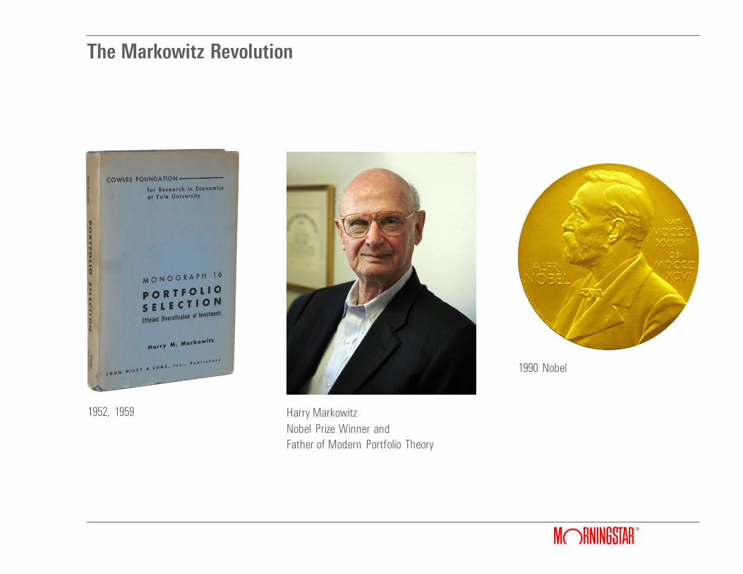
The Markowitz Revolution

1952, 1959 Harry Markowitz

Nobel Prize Winner and

Father of Modern Portfolio Theory

1990 Nobel

5

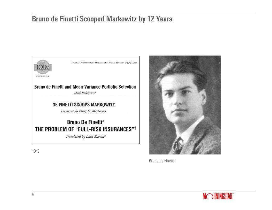
1940

Bruno de Finetti

Bruno de Finetti Scooped Markowitz by 12 Years

Asset Allocation as an Investment Paradigm

6

g In our analyses the [portfolio weights] might represent individual securities or they might represent aggregates such as, say, bonds, stocks and real estate. —Harry Markowitz (Markowitz 1952)

g I think the most important thing that happened between 1959 and the present is the notion of doing your analysis on asset classes in the first instance. This has become part of the infrastructure that we now rely on. In 1959, I had a theory. I had a rationale, and so on. Now, we have an industry. —Harry Markowitz, (Markowitz, Savage, and Kaplan 2010)

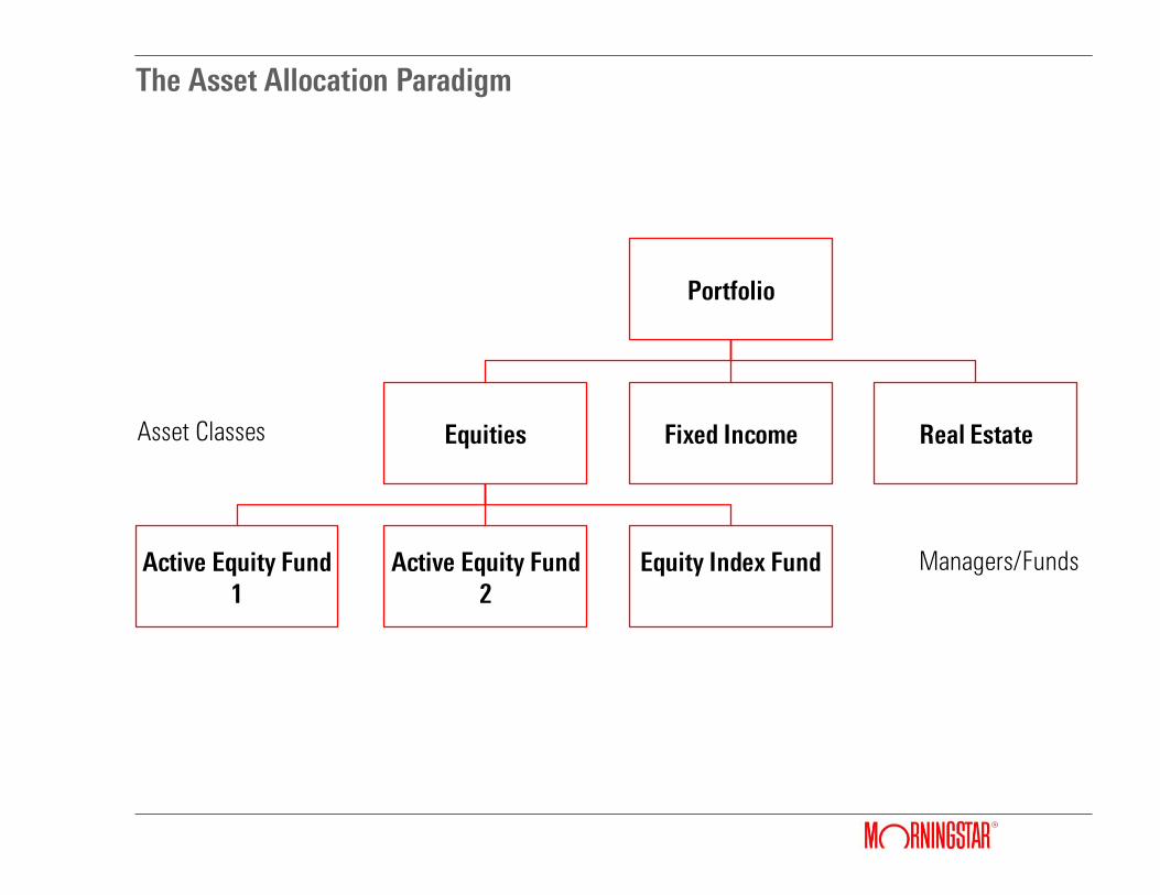
The Asset Allocation Paradigm

Portfolio

Equities

Active Equity Fund 1

Active Equity Fund 2

Equity Index Fund

Fixed Income Real Estate Asset Classes

Managers/Funds

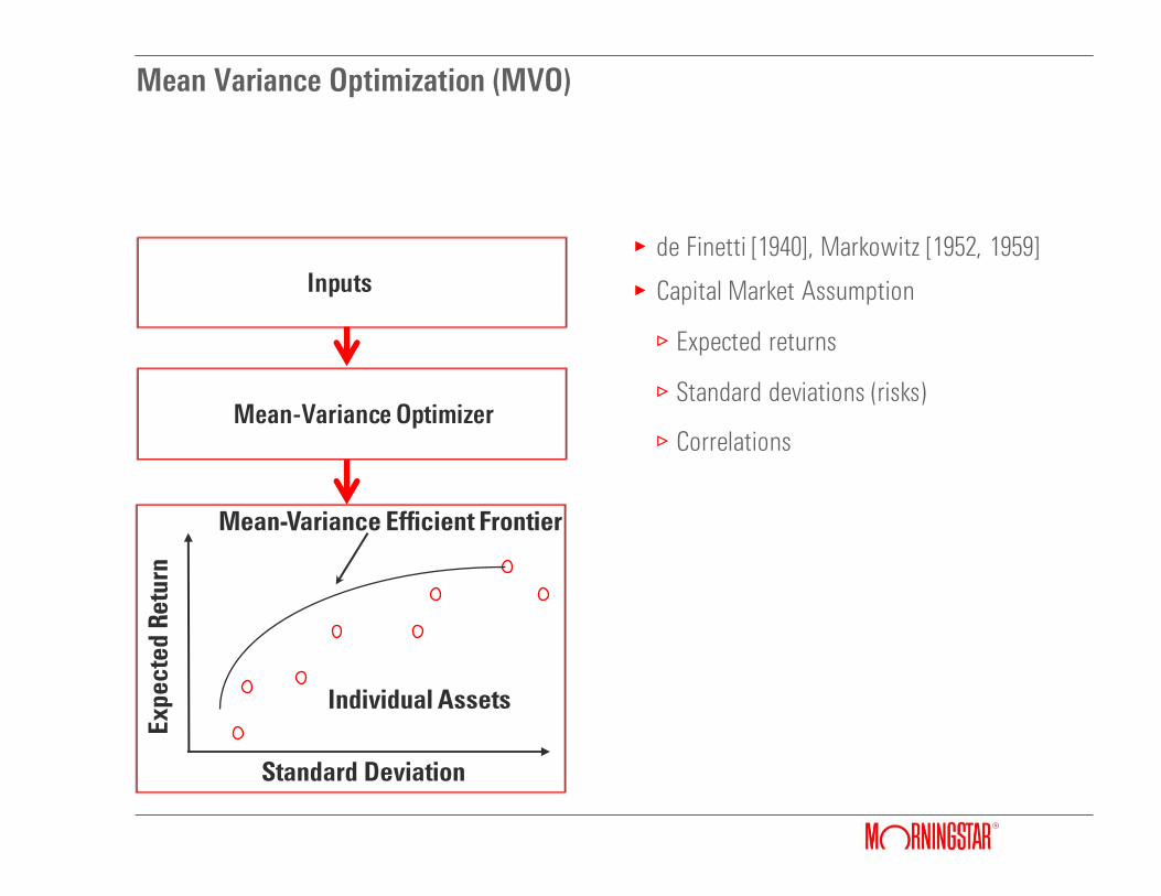
Mean Variance Optimization (MVO)

g de Finetti [1940], Markowitz [1952, 1959]

gCapital Market Assumption

/Expected returns

/Standard deviations (risks)

/Correlations Mean-Variance Optimizer

Inputs

Ex

pe

cte

d R

etu

rn

Mean-Variance Efficient Frontier

Individual Assets

Standard Deviation

The Capital Asset Pricing Model (CAPM)

9

gDeveloped independently by Jack Treynor (1961, 1962), William Sharpe (1964), John Lintner (1965a,b) and Jan Mossin (1966)

gSharpe shared 1990 Nobel Prize with Harry Markowitz, and Merton Miller

g The CAPM is inspired by Markowitz’s MVO model, but is quite distinct from it

gMost importantly, MVO is a normative theory, while the CAPM is a positive theory

g “[A] positive science may be defined as body of systematized knowledge of what is;

a normative … science as a body of systematized knowledge of what ought to be…”

— John Neville Keynes, The Science and Method of Political Economy, p. 22, 1917 [1890]

The CAPM: Assumptions and Conclusions

10

gAssumptions

/Taxes, transaction costs, and other real world considerations can be ignored

/All investor uses MVO to select portfolios

/All investors have the same forecasts; i.e., the same capital market assumptions

/All investors can borrow and lend at the same risk-free rate without limit

gConclusions

/The market portfolio is on the efficient frontier

/Each investor combines the market portfolio with the risk-free asset (long or short)

/MVO not needed!

/The expected excess return of each security is proportional to its systematic risk with respect to the market portfolio (beta)

/But these conclusions do not follow if the fourth assumption does not hold (Markowitz 2005)

Contrarian Asset Allocation

11

g The CAPM is not contrarian

/Hold the market portfolio in combination with long or short cash

/Only need to rebalance cash/risky portfolio combination, not the risky asset classes

/Can be generalized with Adaptive Asset Allocation (Sharpe 2010)

gStrategic Asset Allocation is contrarian

/Pick fixed asset class weights, perhaps using MVO

/Regularly rebalance to fixed weights by selling winners and buying losers

g Tactical Asset Allocation is even more contrarian

/Re-estimate short-term expected returns on a regular basis

/As short-term expected returns change, reset weights, perhaps using MVO

/Since short-term expected returns tend to rise (fall) as market values fall (rise), TAA can be highly contrarian

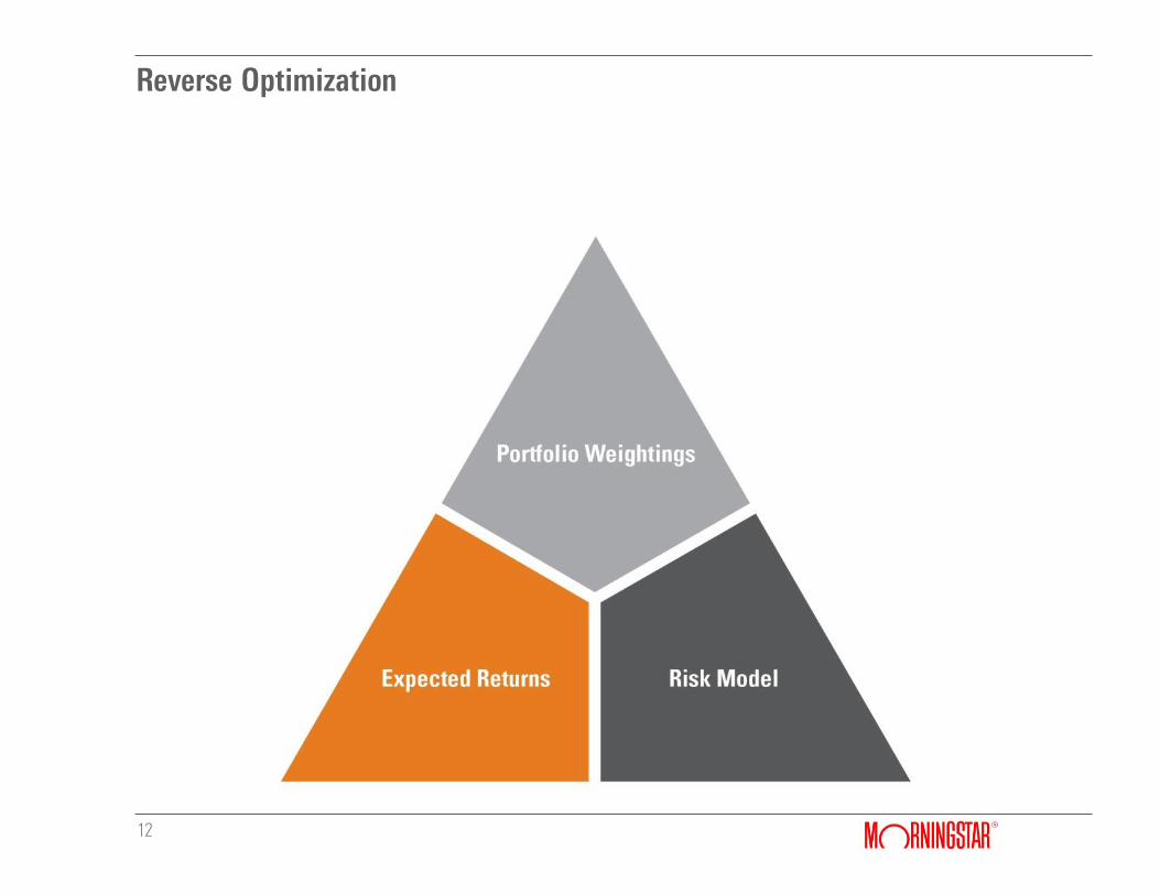
Reverse Optimization

12

The Black-Litterman Model of Expected Returns (1992)

13

g First perform reverse optimization on the market portfolio to get a starting point

g Express views on expected returns with confidence levels

/For example: The expected return on Canadian stocks is 2% higher than that of U.S. Stocks, with a confidence of 60%

gCombine the views with the results of reverse optimization using the Black-Litterman formula to come up with new expected returns

gApply MVO using the new expected returns

g The resulting portfolio, relative to the market portfolio, will tilt towards those asset classes with higher expected returns, and away from those will lower expected returns

g If the views are short-term and updated regularly, the Back-Litterman model is an implementation of TAA

Portfolio Insurance

14

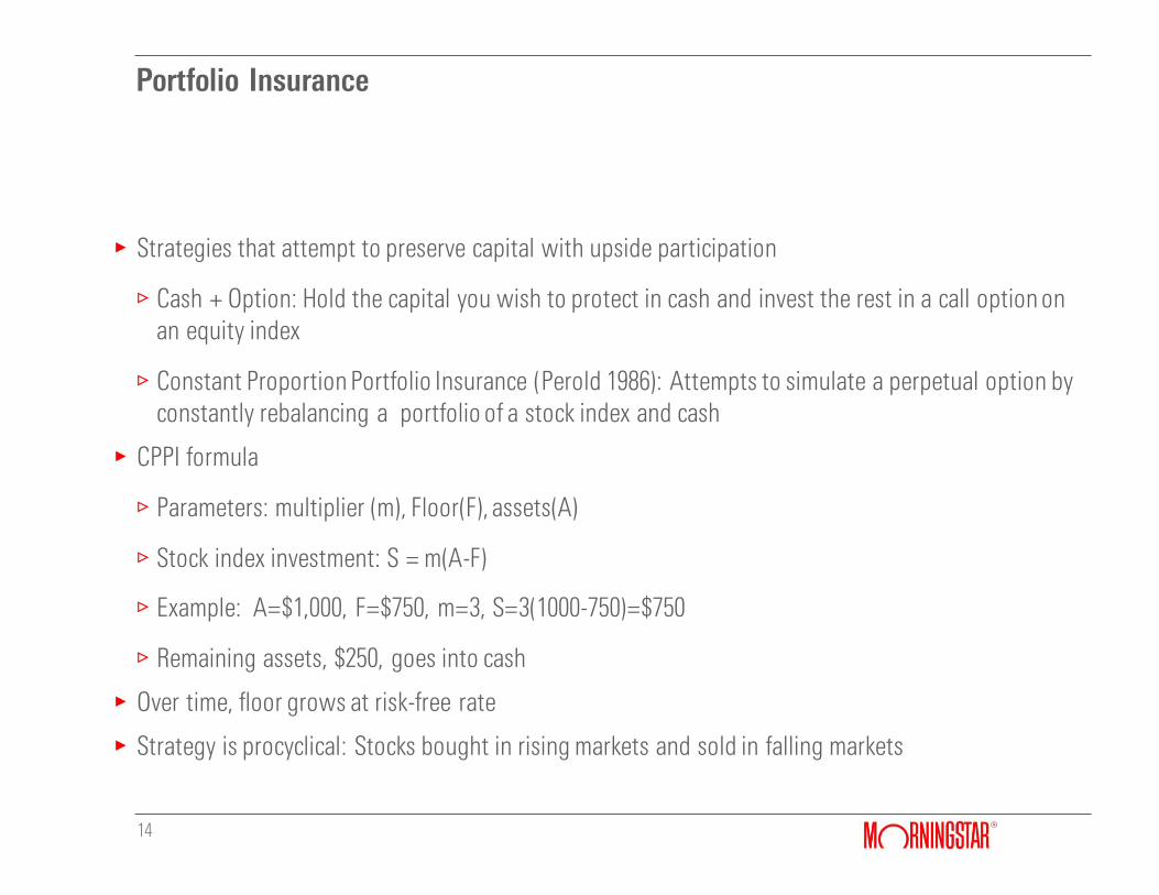
gStrategies that attempt to preserve capital with upside participation

/Cash + Option: Hold the capital you wish to protect in cash and invest the rest in a call option on an equity index

/Constant Proportion Portfolio Insurance (Perold 1986): Attempts to simulate a perpetual option by constantly rebalancing a portfolio of a stock index and cash

gCPPI formula

/Parameters: multiplier (m), Floor(F), assets(A)

/Stock index investment: S = m(A-F)

/Example: A=$1,000, F=$750, m=3, S=3(1000-750)=$750

/Remaining assets, $250, goes into cash

gOver time, floor grows at risk-free rate

gStrategy is procyclical: Stocks bought in rising markets and sold in falling markets

The Life, Death, and Re-emergence (of Sorts) of CPPI

15

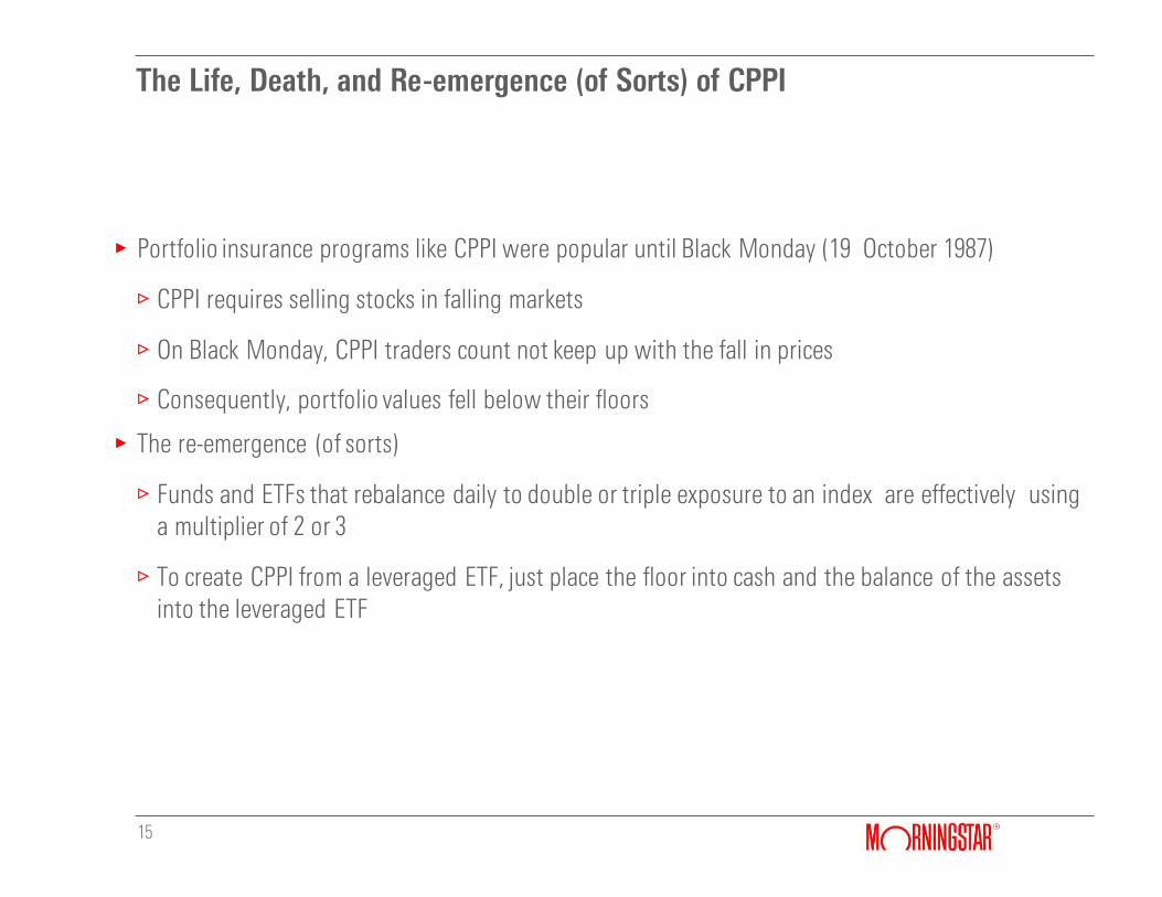
g Portfolio insurance programs like CPPI were popular until Black Monday (19 October 1987)

/CPPI requires selling stocks in falling markets

/On Black Monday, CPPI traders count not keep up with the fall in prices

/Consequently, portfolio values fell below their floors

g The re-emergence (of sorts)

/Funds and ETFs that rebalance daily to double or triple exposure to an index are effectively using a multiplier of 2 or 3

/To create CPPI from a leveraged ETF, just place the floor into cash and the balance of the assets into the leveraged ETF

Sharpe’s Equilibrium View

16

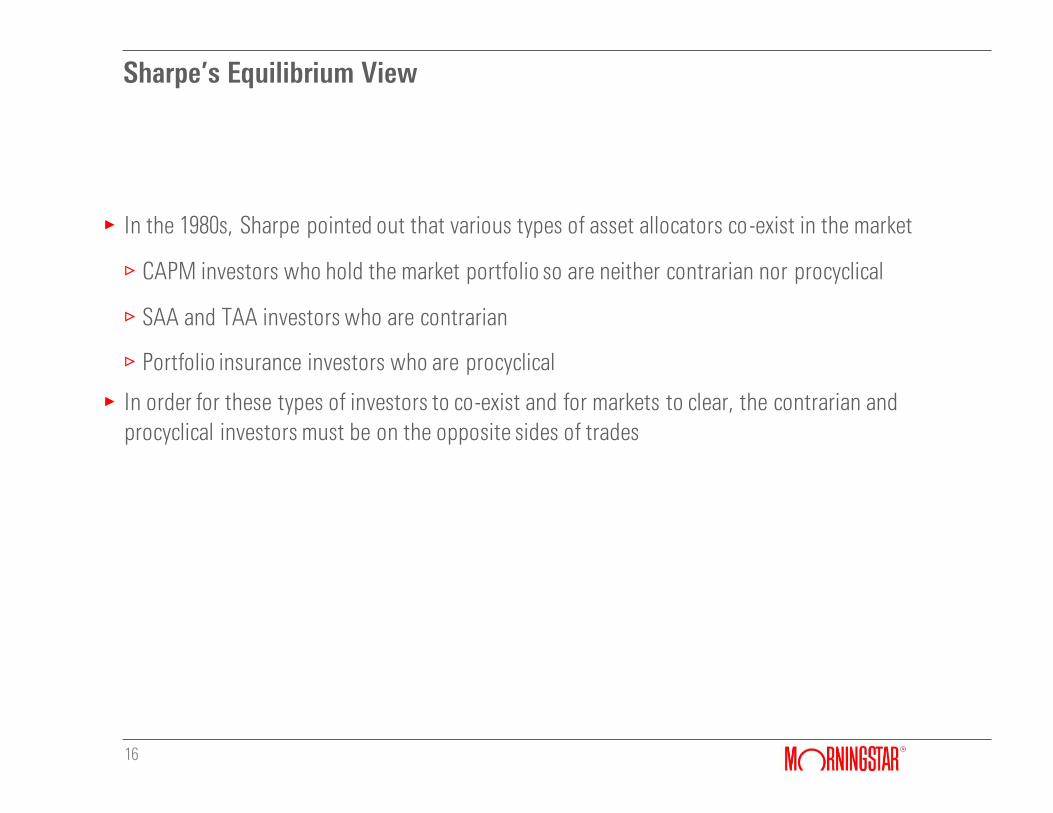
g In the 1980s, Sharpe pointed out that various types of asset allocators co-exist in the market

/CAPM investors who hold the market portfolio so are neither contrarian nor procyclical

/SAA and TAA investors who are contrarian

/Portfolio insurance investors who are procyclical

g In order for these types of investors to co-exist and for markets to clear, the contrarian and procyclical investors must be on the opposite sides of trades

“Post Modern” Portfolio Theory (1991)

17

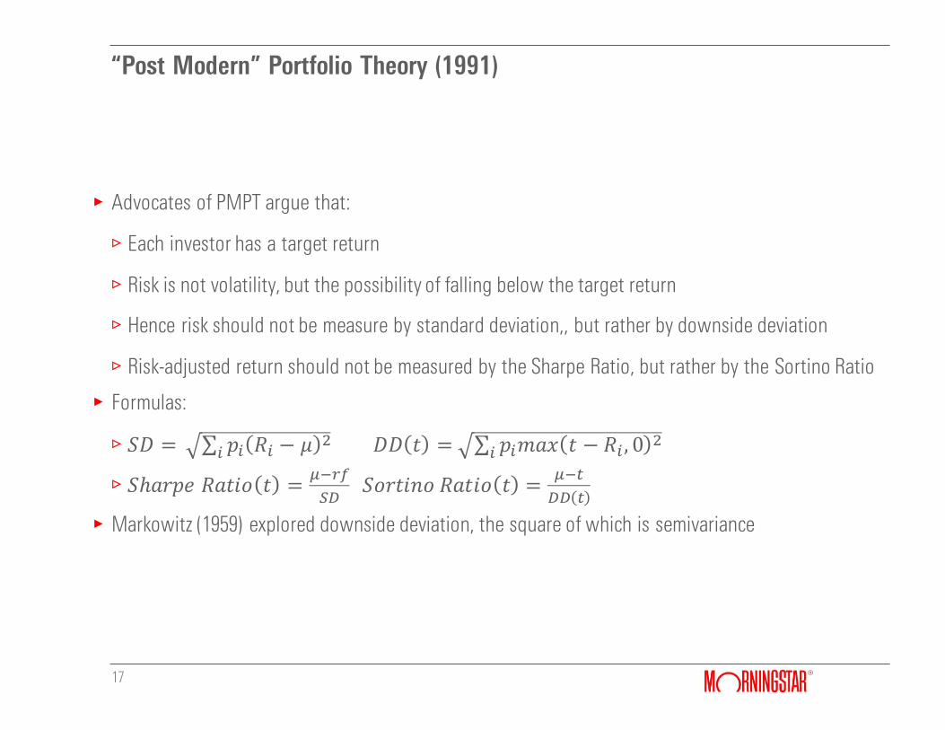
gAdvocates of PMPT argue that:

/Each investor has a target return

/Risk is not volatility, but the possibility of falling below the target return

/Hence risk should not be measure by standard deviation,, but rather by downside deviation

/Risk-adjusted return should not be measured by the Sharpe Ratio, but rather by the Sortino Ratio

g Formulas:

/𝑆𝐷 = 𝑝𝑖 𝑅𝑖 − 𝜇2

𝑖 𝐷𝐷 𝑡 = 𝑝𝑖𝑚𝑎𝑥 𝑡 − 𝑅𝑖 , 02

𝑖

/𝑆ℎ𝑎𝑟𝑝𝑒 𝑅𝑎𝑡𝑖𝑜 𝑡 =𝜇−𝑟𝑓

𝑆𝐷 𝑆𝑜𝑟𝑡𝑖𝑛𝑜 𝑅𝑎𝑡𝑖𝑜 𝑡 =

𝜇−𝑡

𝐷𝐷 𝑡

gMarkowitz (1959) explored downside deviation, the square of which is semivariance

Risk Measurement in the Modern Era: VaR & CVaR

18

gValue at Risk (VaR) describes the tail in terms of how much capital can be lost over a given period of time

gA 5% VaR answers a question of the form:

/Having invested 10,000 dollars, there is a 5% chance of losing X dollars in T months. What is X?

gConditional Value at Risk (CVaR) is the expected loss of capital should VaR be breached

gCVaR>VaR

gVaR & CVaR depend on the investment horizon

.

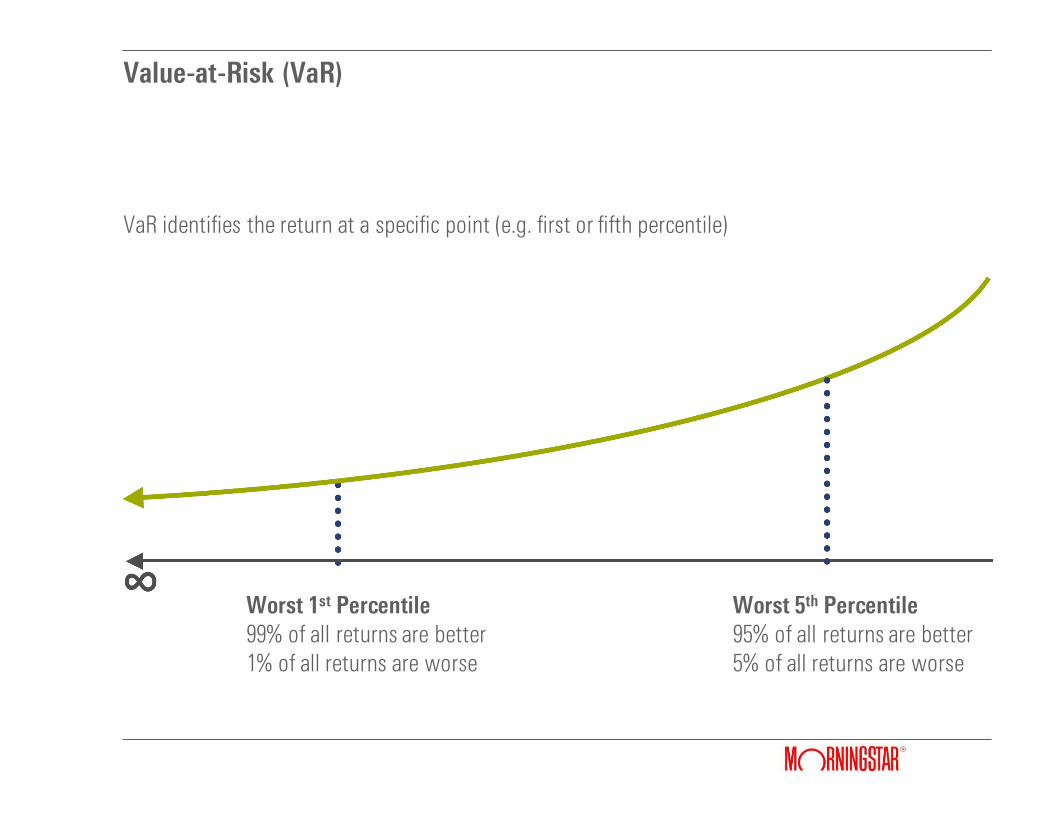
VaR identifies the return at a specific point (e.g. first or fifth percentile)

Value-at-Risk (VaR)

Worst 5th Percentile 95% of all returns are better 5% of all returns are worse

Worst 1st Percentile 99% of all returns are better 1% of all returns are worse

CVaR identifies the probability weighted return of the entire tail

Conditional Value-at-Risk (CVaR)

Worst 5th Percentile 95% of all returns are better 5% of all returns are worse

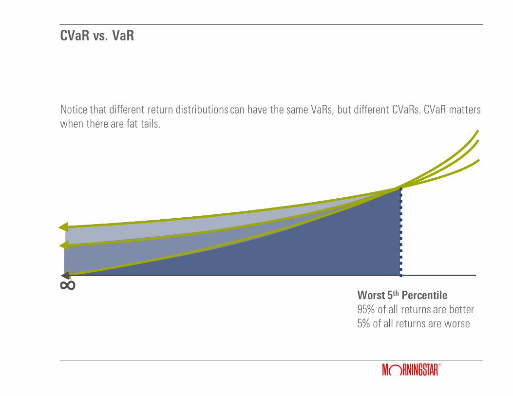
Notice that different return distributions can have the same VaRs, but different CVaRs. CVaR matters when there are fat tails.

CVaR vs. VaR

Worst 5th Percentile 95% of all returns are better 5% of all returns are worse

Fat Tails

Monthly Returns on the S&P 500, 1926-2014, Lognormal Fit

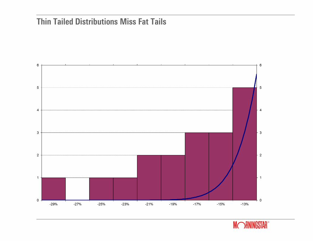
Thin Tailed Distributions Miss Fat Tails

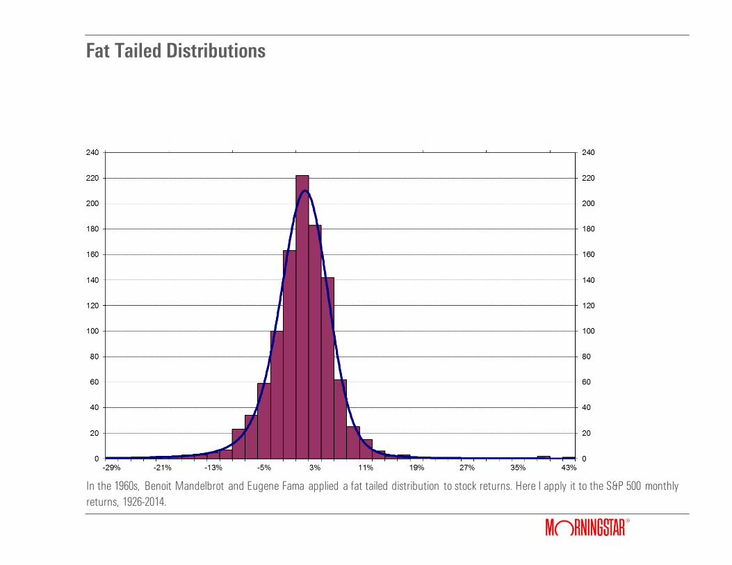
In the 1960s, Benoit Mandelbrot and Eugene Fama applied a fat tailed distribution to stock returns. Here I apply it to the S&P 500 monthly

returns, 1926-2014.

Fat Tailed Distributions

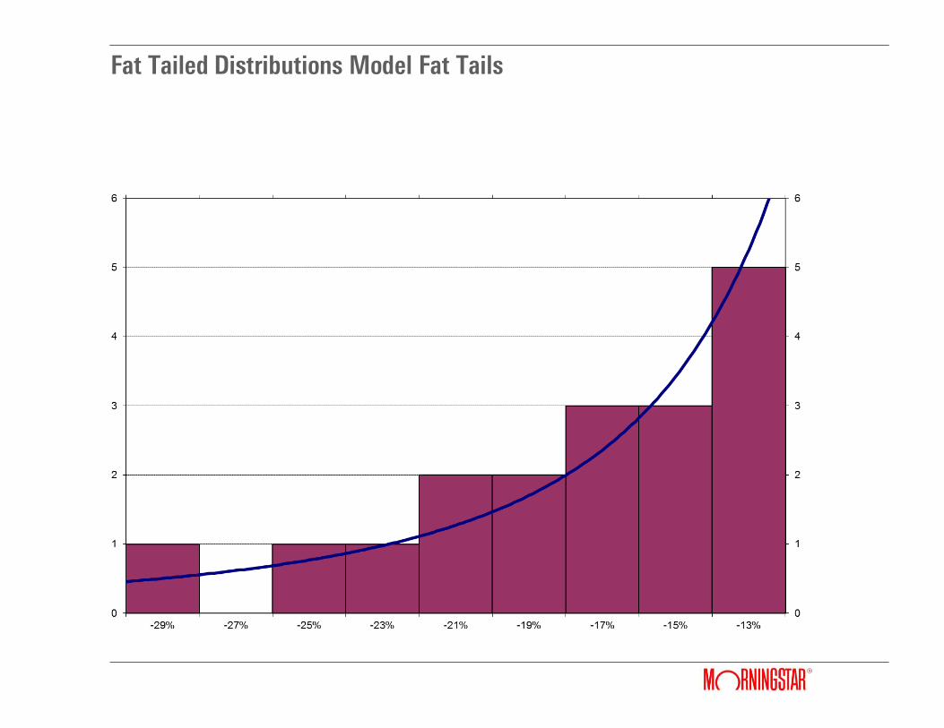
Fat Tailed Distributions Model Fat Tails

The Kelly Criterion

26

g J. L. Kelly (1956) proposed that the optimal way to accumulate wealth over the very long run is to maximize the rate of growth of your portfolio

g This is equivalent to maximizing the expected geometric mean

gMarkowitz (1959, 1979, 2010) has promoted the expected geometric mean as a portfolio selection criterion

gSince the output of MVO is single-period expected return and standard deviation, Markowitz (and Levy 1979) developed several methods for estimating expected geometric mean from expected return and standard deviation

g In Markowitz 2.0 (Kaplan and Savage 2010), expected geometric mean is calculated directly from simulated returns representing various scenarios

.

Markowitz 2.0

27

g In Mankowitz 1.0 (MVO), risk is measured by standard deviation and reward is single period expected return

g In Markowitz 2.0, risk can be measured by any of several measures, including:

/Standard deviation

/Downside deviation

/CVaR

g In Markowitz 2,0, reward can be measured by:

/Single period expected return

/Expected geometric mean

g In Markowitz 2.0 all calculations are made directly from simulated returns representing various scenarios which can number in the thousands

gReturns can be simulated using any distribution, including fat tailed, using Monte Carlo

.

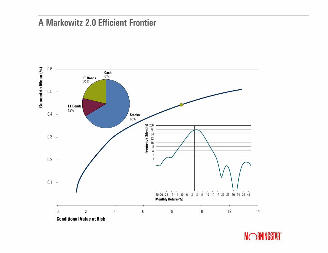
A Markowitz 2.0 Efficient Frontier

Read More About Markowitz 2.0 and Other Ideas in My Book

g “The breadth and depth of the articles in this book suggest that Paul Kaplan has been thinking about markets for about as long as markets have existed.” -Laurence B. Siegel, from the foreword