The Gender Wage Gap and Sample Selection

via Risk Attitudes

Seeun Jung∗†

Paris School of Economics

June 2013

Abstract

This paper investigates a new way to decompose the gender wage gap with the

introduction of individual risk attitudes using representative Korean data. We esti-

mate the wage gap with correction for the selection bias, which latter results in the

overestimation of this wage gap. Female workers are more risk averse. They hence

prefer working in the public sector, where wages are generally lower than in the pri-

vate sector. Therefore, our observation of the gender wage differential based on the

normal Mincerian wage equation is overestimated. Our (corrected) wage differential

is significantly reduced (by from 3% to 8% points) by applying the Switching Re-

gression Model and Lee’s polychotomous selection correction. Self-selection based

on risk attitudes therefore explains, in part, what is popularly perceived as gender

discrimination.

JEL Classification: J24; J31; D81; C52

Keywords: Occupational Choice; Gender Wage Gap; Risk Preference; Selection

Bias

∗E-mail: sejung (at) ens.fr†The author is grateful for comments by Andrew E. Clark, Luc Arrondel, Fabrice Etile, Thomas

Dohmen, Ronald Oaxaca, Chung Choe, seminar participants at ISER & GCOE Behavioral Economics

Joint Seminar of Osaka University, at CEPS/INSTEAD seminar in Luxembourg and the conference of

EALE 2011. The financial support of CEPREMAP is gratefully acknowledged.

1

1 Introduction

Many factors can affect an individual’s decisions about economic issues. In human-capital

theory, risk is involved when students make education decisions, such as weighing random

future income against an additional year of education. In the labor market, some people

choose to endure longer periods of unemployment in order to obtain better wages and

working conditions, while some prefer to exit unemployment sooner despite lower wages.

Others prefer lower wages and safer public-sector pension and social security plans to

higher wages and riskier private-sector pension and social security plans.

A number of reasons may underlie these choices. First, markets might not clear such

that firms do not offer the same wage profiles to identical workers. Second, there could

be individual heterogeneity in the decision-making process. Even when all observable

factors are controlled for - such as gender, age, wealth, region, etc - there are still signif-

icant differences in outcomes. This suggests the presence of unobservable factors behind

individual heterogeneity and firm behavior.

Murphy et al. (1987) and Moore (1995) show that job sectors with higher unemploy-

ment and greater risk tend to have higher wages. Hence, job-sorting decisions may well

vary with individuals’ attitudes to risk. More recent work such as Hartog et al. (2003)

also shows that jobs with greater risk are paid higher wages, contributing to the theory

of compensating wage differentials. Workers who are more willing to accept a certain

number of dollars for a given increase in risk are more likely to choose to work in riskier

jobs than those who are less inclined to make a trade-off between wages and risk. While

job-sector choice is sensitive to differences in risk attitudes, it is a priori also strongly

correlated with education decisions.

Measuring attitudes to risk is, however, a delicate task, and there have been various at-

tempts to find the right kind of subjective self-reported variables which accurately reflect

risk aversion. Feinberg (1977) and Hersch and Viscusi (1990) study the use of seatbelts

and smoking behavior. Ekelund et al. (2005) use a psychometric variable measuring harm

avoidance as an indicator of risk attitudes. They find that agents with a higher harm-

avoidance score (i.e. less risk averse) are more likely to become self-employed, which

is considered riskier than being employed as a wage earner. In an experimental study,

Dohmen et al. (2005) show that measures of subjective risk attitudes, such as self-reported

risk aversion and lottery questions, provide a valid predictor of actual risk behavior.

Dohmen and Falk (2011) build upon these results and use self-reported risk aversion in

the German Socioeconomic Panel to see whether risk preferences explain how individuals

are sorted into occupations with different earnings variation. Furthermore, Luechinger

2

et al. (2007) and Pfeifer (2011) analyze selection in public-sector employment, and Grund

and Sliwka (2006) and Cornelissen et al. (2011) study pay-for-performance schemes. All

conclude that risk-averse workers have a greater preference for non-competitive working

environments. Pissarides (1974) presents a theoretical model explaining that risk-averse

workers have lower reservation wages. This relationship is demonstrated empirically by

Pannenberg (2007). Similarly, Goerke and Pannenberg (2008) show that there is a neg-

ative relationship between risk aversion and union membership.

Given that job sorting matters in terms of the position actually held in the labor

market, there is good reason to wonder whether the job-sorting decision interacts with

the gender disparity observed on the labor market. Although the gender bias in education

has been reduced and the education gap between men and women has narrowed in recent

decades Arnot and Weiner (1999), there is still concern over the considerable wage gap

and other kinds of gender-based discrimination on the labor market. In a move to explain

these findings, Croson and Gneezy (2009) and Bertrand (2011) argue that women may

be more risk averse and less competitive than men. More interestingly for our question,

Gneezy et al. (2003), Niederle and Vesterlund (2007) and Croson and Gneezy (2009) all

suggest that differences in risk attitudes might partly explain the gender gap in labor-

market outcomes. Similarly, Barsky et al. (1997), Dohmen and Falk (2011) and Bonin

et al. (2007) show that job-sector selection and wages are correlated with risk attitudes.

Here, then, lies our centre of interest. The gender wage gap is still an interesting issue

for labor economists and policymakers. In many countries, even developed countries like

Sweden where gender rights are believed to be the most equal in the world, gender wage

differentials are often observed. Labor economists analyze this phenomenon and define the

gender wage gap as “discrimination” if it occurs for equally-productive workers (Becker

(1993)). A huge body of literature has been produced in this field to examine the wage

gap and discrimination following the seminal paper of Oaxaca (1973). The raw wage gap

is decomposed into two parts: one explained by human capital and endowments, and the

other unexplained, which is often deemed to be discrimination. Empirical estimations of

wages with human capital commonly use a Mincerian wage equation (Mincer (1974)), in

which the logarithm of wage is regressed on observable socio-demographic variables such

as gender, schooling, age, etc. In this model, however, concerns may arise in the event

of selection issues or omitted variable bias: what would the level of wages have been

in the absence of discrimination? A number of contributions have attempted to correct

this selection bias, mainly based on the selection of labor-market participation (Newman

and Oaxaca (2004)). We here instead consider sector selection (followed by participation

selection) to decompose the gender wage gap, considering selection via individual risk

3

attitudes.

This paper shows how female workers appear to choose to work in the lower-paid

public sector, and how individual risk attitudes can play a role in this decision-making

process. It goes on to explain the reduced gender wage gap by developing an appropriate

sample-selection model. The remainder of the paper is organized as follows. Section

2 introduces the simple conceptual framework behind the idea, and then presents the

analytical framework with the data description in Section 3. Section 4 shows the empirical

results obtained from testing the impact of risk aversion on job sorting and the gender

wage gap with corrected selection bias. Last, Section 5 concludes.

2 Conceptual Framework

Public-sector jobs are often considered to be safer in terms of their associated benefits,

job stability and security. However, they also pay less than private-sector jobs, where

workers obtain a wage premium for taking risks such as higher job separation rates and

fewer or lower-quality benefits. For this reason, we might expect risk-averse workers to

prefer public-sector stability over private-sector wage volatility and a greater probability

of unemployment. In addition, female workers are more sorted into the public rather

than the private sector, which might be explained by different risk-attitudes by gender.

This section introduces some simple occupational self-sorting concepts in terms of

attitudes towards risk.

2.1 Risk-Averse Workers’ Preference for the Public Sector

Here, we present a simple conceptual framework about risk averse workers’ preference of

working in the public sector. Let’s start with a risk neutral agent. The agent can decide

whether to work in the private sector with high wage W1 and high risk of getting fired,

or to work in the public sector with lower wage W2 but low risk. The wage with risk

premium to offset the job-security risk in the private sector is greater than the wage in

the public sector. Then, in the private sector, the agent is facing the risk of getting fired

with the job separation rate λ , in which case he/she will earn the unemployment benefit

W3 which is lower than the wage of the public sector. We assume that in public sector

there is no risk to be fired once a worker is hired.

Then, now we can get the optimal job separation rate where the agent switch his/her

decision between the public sector and the private sector. Taking the risk neutral agent

first, as his/her utility function is linear to the wage, the job separation rate where the

4

agent would switch from the private sector to the public sector would be:

λ∗ =W1−W2

W1−W3

calculated from the indifferent condition of the expected utility between working in the

public sector and working in the private sector

U [W2] = λU [W3] + (1− λ)U [W1]

W2 = λW3 + (1− λ)W1

Now, we define the optimal job-staying rate which is simply the probability of not getting

fired for risk neutral agent is:

P ∗ = 1− λ∗ = 1− W1−W2

W1−W3=W2−W3

W1−W3

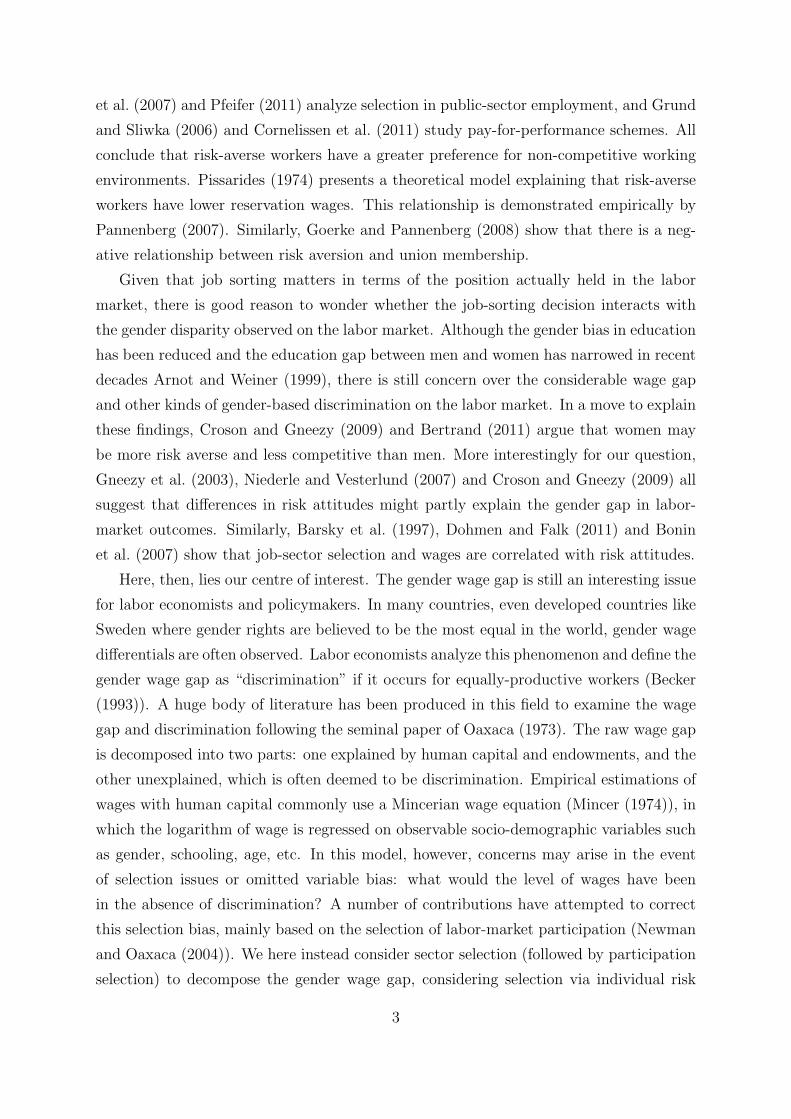
Figure ??Fig:sector1 illustrates the risk neutral agent’s utility function. At the optimal

level of job-staying rate (P ∗ = 1- job separation rate λ), the agent switch the job sector.

Risk Neutral Agent’s optimal strategy with respect to P variation

- 0 ≤ P < P ∗, λ∗ < λ ≤ 1 : U [W2] > λU [W3] + (1 − λ)U [W1] : Always Prefers

Working in the Public

- P = P ∗, λ = λ∗ : U [W2] = λU [W3] + (1 − λ)U [W1] : Indifferent between the

Public Sector and the Private Sector

- P ∗ < P ≤ 1, 0 ≤ λ < λ∗ : U [W2] < λU [W3] + (1 − λ)U [W1] : Always Prefers

Working in the Private

The incentives to work in the public can be found in the lower triangle, where the agent

always decides to work in the public sector, while the incentives to work in the private

sector are in the upper triangle, where he/she always prefers working in the private sector.

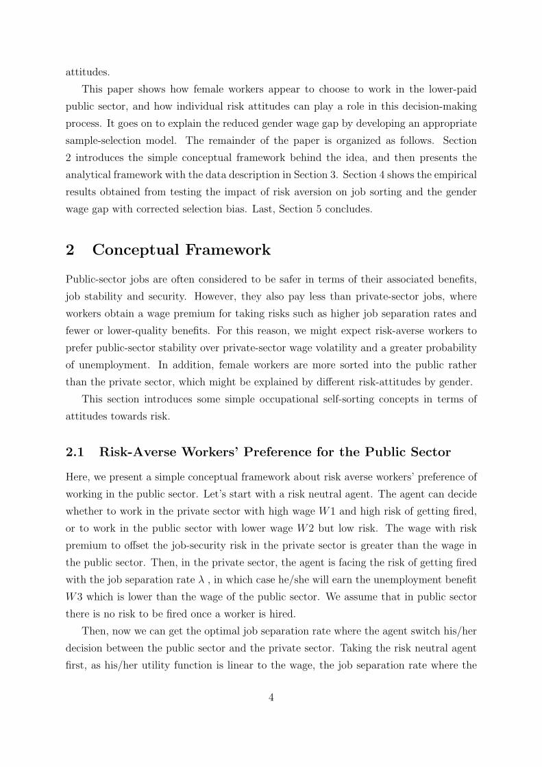
Now, we introduce two different types of agents-risk averse and risk seeking- in addi-

tion to the risk neutral agent. Figure ??Fig:sector2 draws the utility functions for each

agent: risk neutral agent has linear utility function, risk averse agent has concave utility

function, and risk seeking agent has convex function with respect to wealth. Given that

we now know the optimal level of job-staying rate P ∗ = P (RN)∗ for risk neutral agent,

we can graphically get the optimal level of job-staying rate for risk seeking agent P (RS)∗

and risk averse agent P (RA)∗. Due to its concavity (convexity) of the utility function

for risk averse (seeking) agent, the optimal job-staying rate of switching from working

in the public sector to working in the private is higher (lower) than that of risk neutral

5

W3 W2 W1

W3

W2

W1

Wealth

Risk

Neu

tral

Age

nt's

Util

ity

Working in PrivateIncentive

IncentiveWorking in

P*

P=0

P=1

0 < P < P*

P* < P < 1

Choose Public

Choose Private

Public

Figure 1: Public or Private? for Risk Neutral Agent

agent. In other words, risk averse agent needs to have lower job separation rate (higher

job-staying rate) to bear the potential risk of getting fired in the private sector than the

risk neutral agent, whereas risk seeking agent can take higher risk of getting fired at

the higher monitoring rate as he/she would value more on higher wage. Therefore, the

switching job-staying rate for each agent is 0 < P (RS)∗ < P (RN)∗ < P (RA)∗ < 1, and

hence, we can infer the relationship between the optimal switching rate P ∗ and the risk

parameter r (the higher r, more risk averse) :

∂P ∗

∂r> 0 → ∂λ∗

∂r< 0

which means, as getting more risk averse, the agent switch from the private sector to the

public sector at lower job separation rate.

2.2 Gender Difference in Expected Returns

Imagine again that there are two types of firms: public and private. The private firm

pays higher wages, but the atmosphere is highly competitive and the job is not secure.

The public firm is relatively relaxed and the job is more secure, but pays a lower wage

than the private firm. Looking at the private firm, we show below that this firm pays

6

P=0 P(RN)* P=1

W1

W2

W3

P = 1 - Monitoring Rate

Utili

ty P*

P=0

P=1

P*(RS) < P(RN)* P(RN)* < P*(RA)

Risk Averse

Risk Seeker

Risk Neutral

Figure 2: Optimal job-staying rate to switch sectors for Risk Averse, Risk Neutral, and

Risk Seeking Agents

7

male workers higher wages than female workers.

There is less guarantee that a woman will return to the job in the competitive firm after

child bearing than to a job in the public sector, where maternity leave is better-accepted.

Assuming that women’s quitting rates from the private firm are higher than men’s due to

their child bearing, following which the private firm may not guarantee keeping their job

positions open (i.e. qf > qm), the expected return for a given period after hiring by gender

with productivity a and hiring cost of c, a > c > 0 (both identical by gender) in the private

firms is the following: Πf = a(1− qf )− cqf < Πm = a(1− qm)− cqm. Therefore, it makes

sense for the private firm to prefer to hire male workers (i.e. male workers’ probability

of being hired is greater than that of female workers). More risk-averse workers set their

reservation wages lower in order to be hired (Pissarides (1974)), whereas less risk-averse

workers have a lower probability of being hired albeit keeping their reservation wage

higher. This leads more risk-averse female workers to accept lower wage offers in the

private firms. Therefore, among female workers in the private firm, risk-averse workers

earn lower wages. This idea ties in with the “statistical discrimination”1 literature, in

that there are different wage profiles emanating from the demand side (firms).

3 Analytical Framework

Bearing in mind the two scenarios in the previous section, we now set up an analyt-

ical framework in order to test them empirically. A number of pieces of work have

investigated whether the gender gap in risk-taking preferences and competitiveness is

significantly different and even innate. Apicella et al. (2008) show that risk-taking in

an investment game with potential real monetary pay-offs correlates positively with sali-

vary testosterone levels and facial masculinity. More recently, Buser (2011) finds that

women are less competitive both when taking contraceptives that contain progesterone

and estrogen and during the phase of the menstrual cycle when the secretion of these

hormones is particularly high. Hormone studies aside, Sutter and Rutzler (2010) exam-

ines the compensation choices of 1,000 Austrian children and teenagers aged 3 to 18,

and finds that the gender gap in competitiveness is already present by age three. In this

paper, therefore, we write risk aversion (showing individuals’ risk attitudes in general) as

a function of being female (F ) : RA = RA(F, ...). Based on Section 2.1, the probability

of choosing to work in the public sector can be written as a function of being female and

1Statistical discrimination is a theory of inequality between demographic groups based on stereotypes

that do not arise from prejudice or racial or gender bias (Phelps (1972))

8

risk aversion Pub = Pub(F,RA(F ), ...). Last, we extend the Mincerian wage equation to

w = w(F, Pub(F,RA(F, ...)), ...).

Therefore, the wage gap across gender can be written as follows.

∆w

∆F=∂w

∂F+

∂w

∂Pub

∆Pub

∆F

=∂w

∂F+

∂w

∂Pub

∂Pub

∂F+

∂w

∂Pub

∂Pub

∂r

∆RA

∆F

Female workers’ lower wages derive from three factors: (1) purely being female (this could

be interpreted as pure market discrimination); (2) female workers’ preference for work in

the public sector irrespective of their risk attitudes or private firms’ preference for hiring

male workers, which prompts women to work in the public sector (section 2.2), and (3)

choosing to work in the public sector and get lower wage due to women’s higher risk

aversion. The sign of each term would be the following:

- ∂RA∂F

> 0 : Women are more risk averse.

- ∂Pub∂RA

> 0 : Risk averse workers prefer to work in the public sector.

- ∂Pub∂F

> 0 : Due to non-pecuniary benefit (guaranteed maternal leave, child care

service), female workers prefer working in the public sector irrespective of risk at-

titudes. Or private firms prefer to hire male workers for their higher expected

returns.

- ∂w∂Pub

< 0 : Risky firms compensate their risk with the risk premium, paying higher

wage to workers.

Therefore, gender wage gap ∆w∆F

that we observe in the labor markets is the composition

of pure female discrimination ∂w∂F

, the gap from female workers’ preference on working in

the public sector ∂w∂Pub

∂Pub∂F

, and the gap from their being risk averse which leads to work

in the public sector and also to get lower wage ∂w∂Pub

∂Pub∂r

∆RA∆F

. In this paper, we attempt

to disentangle the impact of risk aversion on the wage gap, and get the corrected gender

wage gap which comes from market discrimination. The following Figure ??Fig:scheme

illustrates these three factors.

3.1 Selection

The concern often raised with the Mincerian wage equation is that the employment sector

is wage-endogenous. There are omitted variables which could influence both wages and

sector selection. If we do not control for this selection, the results from the wage equations

9

Being FemaleBeing Female

Being Risk AverseBeing Risk Averse

Prefering Public SectorPrefering Public Sector

Getting Lower WageGetting Lower Wage

Figure 3: Graphic Illustration of Female Worker’s Path towards Lower Wage

could be biased. Here we use a risk-attitude variable to correct for selection and obtain

adjusted estimates of the gender wage gap, as risk aversion could determine workers’

employment sector choices.2

3.1.1 Switching Regression Model

Nakosteen and Zimmer (1980) propose a model to address the earnings of migrants and

non-migrants (the move stay model). In our paper, we apply their method to deal

with self-selection. We estimate the earnings for public-sector workers and private-sector

workers separately.

wpub,i = αpub +X ′pub,iβpub + εpub,i : Public Wage Equation

wpri,i = αpri +X ′pri,iβpri + εpri,i : Private Wage Equation

The sector-selection function is:

Pub∗i = δRAi + Z ′iγ + ui : Sector Choice

Pubi = 1 if Pub∗i > 0 : In Public

where Pub∗i is a latent variable such that if Pub∗i > 0 then Pubi takes the value of 1 (choice

of the public sector), otherwise Pubi takes the value of 0 (choice of the private sector);

2Regarding the exclusion restriction, Korean labor market wages are quite rigid once people are

employed and are often not negotiable on entering the market. Therefore, risk aversion can be assumed

to affect wages only in terms of sector selection. However, we will appeal to polychotomous choice

sample-selection models to discuss this issue in the following section.

10

RAi is the variable that captures individual risk attitudes (hereafter risk aversion) and Zi

is a vector of characteristics influencing the employment-sector decision. If we take the

condition Pubi = 1 (i.e. workers in the public sector), the earning equation for workers

in the public sector is as follows:

E(wpub,i|xpub, Pubi = 1) = αpub +X ′pub,iβpub + E(εpub,i|ui > −δRAi − Z ′iγ)

= αpub +X ′pub,iβpub + σεpub,uφ(−δRAi − Z ′iγ)

1− Φ(−δRAi − Z ′iγ)

= αpub +X ′pub,iβpub + σεpub,uφ(δRAi + Z ′iγ)

Φ(δRAi + Z ′iγ)

= E(ypub,i|xi) + σεpub,uλ

where (εpub,i, ui) is joint normal and σεpub,u = Cov(εpub,i, ui). This covariance determines

the effect of selection on the conditional income of workers in the public sector. If ρεpub,u

is significantly different from zero, we cannot ignore the unobservable characteristics that

could affect both selection and earnings. The wage equation for workers in the private

sector can similarly be written as:

E(wpri,i|xi, Pubi = 0) = αpri +X ′pri,iβpri + E(εpri,i|ui ≤ −δRAi − Z ′iγ)

= αpri +X ′pri,iβpri + σεpri,u[−φ(−δRAi − Z ′iγ)

Φ(−δRAi − Z ′iγ)]

= αpri +X ′pri,iβpri − σεpri,uφ(δRAi + Z ′iγ)

1− Φ(δRAi + Z ′iγ)

Furthermore, we can calculate the hypothetical expected log wage (i.e. public-sector

workers’ expected wages if they worked in the private sector and private-sector workers’

expected wages if they worked in the public sector).

E(wpub,i|xpub, Pubi = 0) = αpub +X ′pub,iβpub − σεpub,uφ(δRAi + Z ′iγ)

1− Φ(δRAi + Z ′iγ)

E(wpri,i|xi, Pubi = 1) = αpri +X ′pri,iβpri + σεpri,uφ(δRAi + Z ′iγ)

Φ(δRAi + Z ′iγ)

3.1.2 Polychotomous Choice Sample Selection Model (Lee (1983))

We now consider the case where people choose from three alternatives; (1) employment in

the public sector, (2) employment in the private sector, and (3) otherwise (unemployed,

inactive, or self-employed). This factors in the possibility that risk aversion could affect

11

wages via one more channel: the reservation wage associated with entering employment.3

Consider the following polychotomous choice model with three categories:

wk = αk + xkβk + ρkuk

s∗k = δRAk + Zkγk + vk

where k = 1, 2, 3 and uk ∼ N(0, 1). McFadden (1974) shows that if vk is i.i.d with a

Gumbel distribution, the probability of individual i choosing j is

Pr(sij = 1) =exp(ηij)

1 +∑3

k=1 exp(ηik)if j > 1

or =1

1 +∑3

k=1 exp(ηik)if j = 1

where ηij = maxk=1,2,3k 6=js∗k − vj.

If we denote J = Φ−1F , the transformed random variable η∗j = Jηs is standard normal.

The bias-corrected wage equation is then

wj = αj + xjβj − σjρjφ(Jj(δRAj + Zjγ))/Fj(δRAj + Zjγ) + εj

under the assumption that uk and η∗j are joint normally distributed, E(εj|jis chosen) = 0,

φ is a standard normal density function, σj is the standard deviation of the disturbance

uj, and ρj is the correlation coefficient of uj and η∗j . The conditional variance of εj is

V ar(εj|l = j) = σ2j − (σjρj)

2[Jj(δRAj + Zjγ) + φ(Jj(δRAj + Zjγ)/Fj(δRAj + Zjγ)]

×φ(Jj(δRAj + Zjγ)/Fj(δRAj + Zjγ)

4 Data and Results

4.1 Data

This paper uses data from Korea where the gender gap is still an important labor market

issue. Even though Korea’s economy has grown remarkably over the past few decades,

its gender wage gap remains the largest among member countries of the Organization for

Economic Co-operation and Development (OECD). Data from the OECD’s 2009 Annual

Report show that male workers in Korea are paid 40 percent more than their female

counterparts. This is the widest gender wage gap of the 30 OECD member economies,

3See Pissarides (1974)

12

being over twice the OECD average of 18.8 percent.

Our data comes from the Korean Labor & Income Panel Study published by the Korean

Labor Research Institute. This survey was first launched in 1998 and now has more than

10 waves, being carried out once a year. It covers 5,000 households and their members

(11,855 individuals in all) who currently live in Korea. These panel data are interesting

in that they contain questions on risk attitudes and many different elements of job and

life satisfaction. For this paper, we restrict the sample to 4,208 individuals in the one

wave (2007) in which the risk questions are available, and also only consider individuals

who are currently employed as wage earners in order to deal with labor-market sector

selection. In the Korean sample, the occupational shares for the 11,855 individuals are

as follows:

Mainly Working (Public, Private, and Self-Employed) 5,927 50.0%

Domestic Work (childcare and family duties) 2,649 22.3%

Students 1,396 11.8%

Other economically inactive 1,883 15.9%

Total 11,855 100.0%

We retain wage earners only (sample size 4,208) for the switching regression model in

order to look at selection between the public and private sectors. The full sample is then

used for the polychotomous selection model when estimating sector selection including

the labor market participation decision. For individual risk attitudes, we construct a

measure from the answers to five lottery-type questions.

Table 1 presents the simple descriptive statistics on wage earners. The proportion of

female workers in the wage-earning segment of the Korean labor market is about 40%.

Figure 3 shows the percentage of women among wage earners in different cohorts. In

Korea, women tend to enter the labor market earlier than men, since men have to serve

two years of national service before entering the labor market. Women’s labor market

participation drops sharply however by the age of 30. This is the age at which they often

get married (Figure 4). Figure 5 depicts the log wage difference between genders in the

different cohorts. There appears to be no difference in terms of wages on entering the

labor market. There is a break point at which male workers start to earn more at the

age of 25-30, which might be the age of ‘marriage’, and the gap grows with age. Marital

status in Korea may therefore be one factor in explaining women’s labor market behavior,

including wages and sectoral choice. However, our data here only covers employees and

not the self-employed, in which sector where there are generally more men. Therefore,

our dataset here does not cover all labor market participation. We can first look at

13

the gender wage differential. On average, women have lower wages (KRW130.61million

monthly),4 fewer years of schooling (12.39 years), and are younger (age 39) than men

(KRW227.57 million, 13.34 years education, age 41). This lower wage could be the result

of both gender discrimination and female workers’ characteristics, such as less education

and a higher proportion of women in the public sector (47% of public-sector workers

are women as opposed to 36% in the private sector), where wages are generally lower

(KRW207 million in the private sector and KRW140 million in the public sector). In

addition, public-sector workers’ risk aversion5 is higher on average than it is for workers

in the private sector. Women are also found to be more risk averse. We now describe

how risk aversion is measured in our data.

4.2 Measuring Risk Aversion

The Korean Labor & Income Panel Study recently added in a number of pilot questions

on individual risk attitudes. We use the 2007 wave, which contains five lottery questions

that we can use to summarize individual risk-taking attitudes. Each individual is asked

whether they would accept the given lottery or take KRW100,000 (USD 82) in cash, or

whether they are indifferent between the two. The details of the five questions are shown

below:

Number Lottery characteristics Expected Value [Ni] Weight[αi]

1 1/2: KRW150,000, 1/2: KRW50,000 KRW100,000 363 0.155

2 1/2: KRW200,000, 1/2: KRW0 KRW100,000 314 0.179

3 1/5: KRW500,000, 4/5: KRW0 KRW100,000 226 0.249

L 3/5: KRW200,000, 2/5: KRW0 KRW120,000 389 0.145

H 2/5: KRW200,000, 3/5: KRW0 KRW80,000 207 0.272

Here, the first three choices - denoted risk1, risk2, and risk3 - have the same expected

value as the fixed amount of KRW100,000, but differ in their degree of riskiness. Taking

risk2 as the baseline, risk1 is less risky than risk2 while risk3 is riskier. Meanwhile, RiskL

and RiskH have different expected values (KRW80,000 and KRW120,000 respectively).

We use the answers to these five questions to construct a risk-aversion variable, which

may well explain a part of individual heterogeneity. Each question is assigned a value

of 0 if the respondent prefers the lottery, which is regarded as risk-taking, a value of 0.5

if the respondent is ‘indifferent’, and a value of 1 if the lottery is not chosen. Higher

numbers therefore indicate greater risk aversion. Different weights can be assigned to

41 U.S. dollar is approximately 1,100 Korean Won5We discuss the construction of our risk-aversion measure in the following section.

14

these choices depending on the lottery’s expected value. For example, in riskL, saying

‘indifferent’ could also mean ‘risk averse’ as the expected value is less than KRW100,000,

because the distance between the expected value and KRW100,000 could be seen as a

risk premium from choosing the lottery. Equally, choosing the lottery in risk1, 2, and 3

would be assigned the same value of 1 above, but this does not mean that those lotteries

have the same associated levels of risk. We therefore weight each risk variable according

to the inverse of the fraction of people choosing the lottery in order to take this into

account.rai =

∑αiRiski, i = 1, 2, 3, L, andH6

where Riski=0 (prefer lottery: less risk averse), 0.5 (indifferent: risk neutral), 1 (pre-

fer cash: risk averse), and αi is an ad-hoc weight, which is higher for a riskier lottery

choice if that lottery is chosen by fewer people, αi = bi/∑bi, where bi is the inverse of

the proportion of the number of lotteries chosen in each case (i.e. bi =∑Ni/Ni, Ni in

the table shows the number of respondents who prefer each lottery i). The risk aver-

sion measure therefore has the range of [0, 1].7 Each lottery has its own weight, which

is calculated as the inverse of the proportion of people who choose the lottery.8 The

ascending order of risk amongst the five lotteries as subjectively perceived by workers is

L(the least risky)→ 1→ 2→ 3→ H(the most risky)).9

Table 2 shows risk aversion in the different sub-samples: by gender, job sector, edu-

cation, age, and marital status. Female workers are more risk averse than male workers,

and workers in the public sector are more risk averse than those in the private sector.

Employed workers (both in the public and the private) tend to be less risk averse than

those who are in other status (self employed or inactive). In addition, highly-educated

workers tend to be less risk averse than workers who have a high-school diploma. Older

workers (aged over 45) are more risk averse, while marital status is also significantly linked

with risk aversion. We do indeed find a gender difference in attitude towards risk, which

is the basis for the work we carry out here. Figure 6 shows the relationship between risk

6This method was introduced by Sung and Ahn (2007)7A simple aggregation using the same weights for each question was also tested and yielded a fairly

similar picture to that produced by the method used above; these results are available on request.

Alternatively, the Barsky et al. (1997) method could be used. The first three questions would yield 27

categories of different risk attitude-groups.8For example, α1 =

1363

1363+ 1

314+ 1226+ 1

389+ 1207

= 0.155, although results are unchanged with the same

weight (αi = 0.2 for all i’s).9There is an issue regarding the inconsistency of respondent choice. For example, 53 respondents

chose to take lottery 2, but not lottery 1, which is less risky. These inconsistency rates are, however,

typically below 2.5% in this sample and do not change the results much. We have therefore retained all

of the observations regardless of their consistency.

15

aversion and age by gender. Women have a tendency to be more risk averse than men at

all ages. This figure also shows a positive slope, suggesting an age effect on risk aversion.

Figure 7 shows risk aversion/age profile by sector. In common with the gender findings,

public-sector workers’ risk aversion is generally higher than that of private-sector workers

across most cohorts. When we compare risk aversion between the public and private

sectors, female workers continue to report greater risk aversion. However, the gender

difference in terms of risk aversion is larger among private-sector workers (Figure 9) than

in the public sector (Figure 8), which might explain the difference in the gender wage

gap between sectors. This is what we now set out to evaluate using a regression analysis.

4.3 Results

Table 3 presents the results of pairwise correlation matrices for the variables in which we

are interested. The main risk-aversion variable is significantly correlated with wage, gen-

der, employment, sector selection, education, being married, health, and father’s educa-

tion. Female, working in the public sector, and being married are all positively correlated

with risk aversion, while the correlation with wage, employment, education, health, and

father’s education is negative. The signs and significance are in line with human-capital

theory and the literature on risk. Wages are lower for women and in the public sector,

and women are found more in the public sector. These correlations are the starting point

of our analyses.

Table 4 presents the results of various wage equations using two different selection-

correction methods; the Switching Regression Model (Nakosteen and Zimmer (1980))

and Lee (1983)’s polychotomous method. In the Korean sample, female workers earn

about 38% less on average than male workers, controlling for other socio-demographic

variables and a public-sector dummy. Returns to education are about 8%, which is fairly

standard. One interesting point is that public workers earn 26% less than do private-

sector workers.10 Columns 2 and 5 show the wage equations for public-sector workers

and private-sector workers respectively. Female workers in the public sector are still paid

less (32%), but the gap is narrower than in the private sector (41%). This could show

that discrimination is harder to effect in the public sector due to policy and also the

less competitive atmosphere, which makes for more equal wage conditions for men and

women. On the other hand, private firms are more competitive and profit-seeking, which

10However, the picture changes slightly when considering skilled and unskilled work. The private sector

pays higher wages for skilled work, whereas the public sector tends to pay higher wages for unskilled

work. Even so, the private sector still pays more on average than the public sector

16

leads workers to work harder. Female workers tend to be left behind in this working

environment due to childcare and less competitive characteristics, which widens the gen-

der gap. Private firms’ preferences for male workers may contribute to this wider gender

wage gap by offering higher wages to men. Returns to education are also higher in the

private sector. Given a set of individual characteristics, wages are higher in the private-

relative to the public-sector (from a comparison of the two constants: 3.636 vs 3.35).

We now consider the selection model. We first use the Switching Regression Model

(Nakosteen and Zimmer (1980)).11 The results of the selection step are presented in

Column 3 in the second panel. The binary dependant variable is public-sector employ-

ment. As expected, women tend to choose (or to be pushed to choose) the public sector.

Education is positively correlated with selection into public sector. Being married is neg-

atively correlated with the public sector, but not significantly so. Health12 is negatively

and significantly correlated with working in the public sector; workers who are confident

in their health may prefer to work in the private sector. Our variable of interest, risk

aversion is, indeed, positively correlated with public-sector choice: workers with greater

risk aversion are more often found in the public sector. The selection correction reveals

the differences in the gender wage gap in both sectors. Columns 3 and 6 display the

wage equation results with selection correction. In the public sector, the gender gap not

explained by other socio-demographic features falls from 32% to 30%. In the private

sector, the gender gap also drops by 3% (41% to 38%). This correction is meaningful as

the estimated value of rho is significantly different from zero, which proves that there is

indeed a selection issue in the main wage equation. Controlling for risk aversion helps

correct women’s self-selection into the public sector and reduces the pure gender gap that

cannot be explained and is often defined as market gender discrimination. Columns 4

and 7 then present the wage equation results corrected using Lee’s method.13 The second

panel shows the multinomial logit model results for: (1) working in the public sector (in

Column 4); and (2) working in the private sector (in Column 7); with (3) self-employed

or inactive as the reference point. Risk aversion no longer has a significant impact on

working in the public sector. However, it becomes a significant determinant of working

in the private sector: the more risk averse the individual, the less likely they are to be

found in the private sector.

11We use the ‘movestay’ stata command developed by Lokshin and Sajaia (2006) to estimate the

switching regression.12Health is self-reported.13We use the ‘selmlog’ stata command developed by Bourguignon et al. (2007) to estimate the poly-

chotomous choice selection model.

17

Noting that all of the rhos in Table 4 are significantly different from zero, we can

now look at the corrected wage equations in the first panel. The Lee correction in the

public sector (Column 4) actually widens the gender gap by 9% points, as compared

to column 2. This underlines the importance of considering participation as a third

element in labor-market choices, and how this participation decision is related to risk

aversion. The results of the three-category choice model show how the two employment

sectors compare with the reference point: the public-sector estimation results show the

comparison to self-employment and inactivity, and not to the private sector. When

individuals compare the public sector with self-employment or inactivity, the coefficient

on risk aversion is insignificant so that the corrected wage gap will not necessarily fall.

What is more significant here is the private sector. In the selection step, risk aversion is

a key determinant of this choice. This correction in the private sector narrows the gender

wage gap even more than in the Roy switching regression model (from 41% to 24%).

This result confirms that selection is indeed not marginal in the private sector. It also

suggests that the gender wage gap in the private sector is substantially overestimated

without correction. Selection across labor-market sectors depends then on risk-aversion.

In particular, the Lee results suggest that selection into the private sector produces women

who are on average less risk-averse than are the men who choose the private sector. As

risk-aversion is negatively correlated with wages, the correction for selection via risk

reduces the female wage penalty in the private sector.

The selection bias makes the gap wider as women are more risk averse in general.

The gender wage gap in the Korean labor market is then reduced from 38% to 35.5%14

using Roy’s method, and to 28.4%15 using Lee’s method to correct for selection bias.

Table 5 shows the prediction of the expected log wage based on the sample correction

method. Expected wages are calculated for the following: unconditional in the public

sector, unconditional in the private sector, conditional in the public sector with workers

currently working in the public sector, conditional in the private sector with workers

currently working in the public sector, conditional in the public sector with workers

currently working in the private sector, and conditional in the private sector with workers

currently working in the private sector. Given that rho1 is positive and significantly

different from zero, the model suggests that individuals who intentionally choose to work

in the private sector earn lower wages than a random individual from the sample (or

currently working in the other sector) would earn (Row 4 vs Row 6). Yet as rho0 is

140.27(in public)× 0.302 + 0.73(in private)× 0.376 ≈ 0.355150.27(in public)× 0.412 + 0.73(in private)× 0.237 ≈ 0.284

18

also positive and significantly different from zero, individuals who intentionally choose to

work in the public sector earn higher wages than a random individual from the sample

(or currently working in the other sector) would earn (Row 3 vs Row 5).

5 Concluding Remarks

This paper provides some evidence on the impact of risk aversion on labor market behav-

ior. We control for risk attitudes based on hypothetical lottery questions from Korean

labor surveys. We especially look at private-public job sector choice, assuming that the

public sector provides more incentives than the private sector in terms of stability and

job security. The results show that risk aversion is a significant and positive determinant

of public-sector employment choice. That women are more risk averse than men hints

that there could be a link between women’s self-selection and the gender wage gap. We

explain labor market gender discrimination partly by risk aversion using a decomposition

into three channels: (1) being female by itself (this could be interpreted as pure market

discrimination); (2) female workers’ preference for working in the public sector regardless

of their risk attitudes or private firms’ preference for hiring male workers, prompting

women to work in the public sector (Section 2.2); and (3) choosing to work in the public

sector due to women’s higher risk aversion. We then need to correct the wage equation

for selection bias. We show that individual risk attitudes are an important determinant

of labor-market participation choices and also public-private sector choice. The switching

regression model narrows the gender gap in both sectors by about 5% points. In addition,

when we extend our model to the multinomial choice model for the selection step, the

gender gap drops sharply in the private sector while it surprisingly increases in the public

sector. This opposite direction, however, could be explained by the different mechanism

at work when we use the multinomial model with self-employment and inactivity as the

reference category. These findings indicate that the wage gap is not simply a product

of the labor market environment, but also the choices made by women themselves based

on their risk aversion and other preferences. In other words, the wage gap is not only a

result of pure discrimination in the labor market, but also of intrinsic sorting based on

preferences formed by risk attitudes. This could be a new way to explain why female

workers in Korea are paid so much less than their male counterparts.

19

References

Apicella, C. L., A. Dreber, B. Campbell, P. B. Gray, M. Hoffman, and A. C. Little (2008).

Testosterone and financial risk preferences. Evolution and Human Behavior 29 (6), 384

– 390.

Arnot, M., D. M. and G. Weiner (1999). Closing the Gender Gap: Post-war Education

and Social Change. Polity Press, Cambridge, UK.

Barsky, R. B., F. T. Juster, M. S. Kimball, and M. D. Shapiro (1997, May). Preference

parameters and behavioral heterogeneity: An experimental approach in the health and

retirement study. The Quarterly Journal of Economics 112 (2), 537–79.

Becker, G. (1993). Human Capital - A Theoretical and Empirical Analysis with Special

Reference to Education. Chicago University Press, 3rd edition.

Bertrand, M. (2011, October). New Perspectives on Gender, Volume 4 of Handbook of

Labor Economics, Chapter 17, pp. 1543–1590. Elsevier.

Bonin, H., T. Dohmen, A. Falk, D. Huffman, and U. Sunde (2007, December). Cross-

sectional earnings risk and occupational sorting: The role of risk attitudes. Labour

Economics 14 (6), 926–937.

Bourguignon, F., M. Fournier, and M. Gurgand (2007). Selection bias corrections based

on the multinomial logit model: Monte carlo comparisons. Journal of Economic Sur-

veys 21(1), 174–205.

Buser, T. (2011). The impact of the menstrual cycle and hormonal contraceptives on

competitiveness. Working Paper Univ. Amsterdam.

Cornelissen, T., J. S. Heywood, and U. Jirjahn (2011, April). Performance pay, risk

attitudes and job satisfaction. Labour Economics 18 (2), 229–239.

Croson, R. and U. Gneezy (2009, June). Gender differences in preferences. Journal of

Economic Literature 47 (2), 448–74.

Dohmen, T. and A. Falk (2011, April). Performance pay and multidimensional sorting:

Productivity, preferences, and gender. American Economic Review 101 (2), 556–90.

20

Dohmen, T., A. Falk, D. Huffman, U. Sunde, J. Schupp, and G. G. Wagner (2005).

Individual risk attitudes: New evidence from a large, representative, experimentally-

validated survey. Discussion Papers of DIW Berlin 511, DIW Berlin, German Institute

for Economic Research.

Ekelund, J., E. Johansson, M.-R. Jarvelin, and D. Lichtermann (2005, October). Self-

employment and risk aversion–evidence from psychological test data. Labour Eco-

nomics 12 (5), 649–659.

Feinberg, R. M. (1977, August). Risk aversion, risk, and the duration of unemployment.

The Review of Economics and Statistics 59 (3), 264–71.

Gneezy, U., M. Niederle, and A. Rustichini (2003, August). Performance in competitive

environments: Gender differences. The Quarterly Journal of Economics 118 (3), 1049–

1074.

Goerke, L. and M. Pannenberg (2008). Risk aversion and trade union membership.

Discussion Papers of DIW Berlin 770, DIW Berlin, German Institute for Economic

Research.

Grund, C. and D. Sliwka (2006, March). Performance pay and risk aversion. Discussion

Papers 101, SFB/TR 15 Governance and the Efficiency of Economic Systems, Free

University of Berlin, Humboldt University of Berlin, University of Bonn, University of

Mannheim, University of Munich.

Hartog, J., E. Plug, L. Diaz-Serrano, and J. Vieira (2003, July). Risk compensation in

wages - a replication. Empirical Economics 28 (3), 639–647.

Hersch, J. and W. K. Viscusi (1990). Cigarette smoking, seatbelt use, and differences in

wage-risk tradeoffs. Journal of Human Resources 25 (2), 202–227.

Lee, L.-F. (1983). Generalized econometric models with selectivity. Econometrica 51(2),

507–512.

Lokshin, M. and Z. Sajaia (2006, April). Movestay: Stata module for maximum likeli-

hood estimation of endogenous regression switching models. Statistical Software Com-

ponents, Boston College Department of Economics.

Luechinger, S., A. Stutzer, and R. Winkelmann (2007). The happiness gains from sorting

and matching in the labor market. SOEPpapers 45, DIW Berlin, The German Socio-

Economic Panel (SOEP).

21

McFadden, D. (1974). Conditional logit analysis of qualitative choice behavior. Frontiers

in Econometrics , 105–142.

Mincer, J. A. (1974). Schooling, Experience, and Earnings. Number minc74-1 in NBER

Books. New York: Columbia University.

Moore, M. J. (1995, January). Unions, employment risks, and market provision of em-

ployment risk differentials. Journal of Risk and Uncertainty 10 (1), 57–70.

Murphy, K. M., R. H. Topel, K. Lang, and J. S. Leonard (1987). Unemployment, risk, and

earnings: Testing for equalizing wage differences in the labor market. In K. Lang and

J. S. Leonard (Eds.), Unemployment and the Structure of Labor Markets, pp. 103–140.

New York: Basil Blackwell.

Nakosteen, R. and M. Zimmer (1980). Migration and income: the question of self-

selection. Southern Economic Journal 46(3), 840–851.

Newman, S. and R. Oaxaca (2004). Wage decompositions with selectivity corrected wage

equations: A methodological note. Journal of Economic Inequality 2, 3–10.

Niederle, M. and L. Vesterlund (2007, 08). Do women shy away from competition? do

men compete too much? The Quarterly Journal of Economics 122 (3), 1067–1101.

Oaxaca, R. (1973). Male-female wage differentials in urban labor markets. International

Economic Review 14(3), 693–709.

Pannenberg, M. (2007). Risk aversion and reservation wages. IZA Discussion Papers

2806, Institute for the Study of Labor (IZA).

Pfeifer, C. (2011). Risk aversion and sorting into public sector employment. Technical

Report vol. 12(1), pages 85-99, 02, German Economic Review, Verein fur Socialpolitik.

Phelps, E. S. (1972). The statistical theory of racism and sexism. American Economic

Review 62(4), 659–661.

Pissarides, C. A. (1974, Nov.-Dec.). Risk, job search, and income distribution. Journal

of Political Economy 82 (6), 1255–67.

Sung, J. and J. Ahn (2007). Measuring of risk tolerance and its role in choosing self-

employment. KIF 13(1), 125–193.

Sutter, M. and D. Rutzler (2010). Gender differences in competition emerge early in life.

IZA Discuss.Pap 5015 .

22

Figures

Figure 4: Female Participation Figure 5: Marital Status by Age

Figure 6: Gender Wage Gap by Age Figure 7: Risk Aversion Age Profile

Figure 8: Risk Aversion Age Profile by Sec-

tor

Figure 9: Risk Aversion Age Profile by Gen-

der in the Public Sector

23

Figure 10: Risk Aversion Age Profile by

Gender in the Private Sector

24

Tables

Table 1: Descriptive Statistics

Full Sample Male Female Diff Private Public Diff

Age 40.00 40.76 38.81 -1.95*** 41.18 36.74 -4.43***

(11.50) (11.11) (12.01) (10.96) (12.31)

Education 12.95 13.31 12.38 -0.94*** 12.97 12.88 -0.09

(3.19) (3.01) (3.37) (3.25) (3.01)

Female 0.39 0.36 0.47 0.11***

(0.49) (0.48) (0.50)

Wage(mil won) 189.37 227.15 130.58 -96.57*** 207.57 139.26 -68.31***

(189.20) (220.92) (99.44) (208.56) (105.80)

Public 0.27 0.23 0.32 0.09***

(0.44) (0.42) (0.47)

Married 0.74 0.76 0.71 -0.05*** 0.79 0.61 -0.17***

(0.44) (0.43) (0.45) (0.41) (0.49)

Risk Aversion 0.927 0.904 0.963 0.06*** 0.923 0.943 0.020**

(0.25) (0.15) (0.25) (0.007) (0.24) (0.18) (0.008)

N 4208 2563 1645 3085 1123

Notes. Standard errors in parentheses

*: p < 0.10, ** : p < 0.05, *** : p < 0.01

25

Table 2: Risk Aversion Measures

Mean SE Obs

Full Sample 837 0.168 11453

Male 0.814 0.204 5546

Female 0.860 0.122 5907

Diff 0.045*** 0.003

Private 0.816 0.204 3085

Public 0.833 0.171 1123

Diff Public-Private 0.017** 0.007

Inactive or SE 0.847 0.149 7245

Diff Employed-Non emp -0.027*** 0.003

Edu > 12yrs 0.847 0.153 7362

Edu ≤ 12yrs 0.820 0.192 4091

Diff -0.027** 0.003

Age < 45 0.821 0.192 6419

Age ≥ 45 0.859 0.130 5034

Diff 0.038*** 0.003

Not married 0.825 0.182 2931

Married 0.841 0.163 8522

Diff 0.017*** 0.004

Notes. *: p < 0.10, ** : p < 0.05, *** : p < 0.01

26

Table 3: Pairwise Correlation of Variables

Risk Aversion Log Wage Female Employed In Public Education Married Health Father Edu

Risk Aversion 1.000

Log Wage -0.112* 1.000

Female 0.135* -0.410* 1.000

Employed -0.077* 0.000* -0.191* 1.000

In Public 0.037* -0.256* 0.099* 0.000* 1.000

Education -0.117* 0.441* -0.213* 0.238* -0.014 1.000

Married 0.045* 0.121* 0.097* -0.009 -0.177* -0.294* 1.000

Health -0.064* 0.163* -0.116* 0.138* -0.037* 0.339* -0.218* 1.000

Father Edu -0.026* 0.036* -0.021* 0.101* -0.145* 0.027* 0.004 0.007 1.000

Notes. *: p < 0.10

27

Table 4: Switching Regression and Polychotomous Selection Model

Full Sample Public Private

Wage

Correction No No Roy Lee No Roy Lee

Female -0,382*** -0,323*** -0,302*** -0,412*** -0,406*** -0,376*** -0,237***

(0,016) (0,03) (0,032) (0,093) (0,019) (0,021) (0,041)

Education 0,08*** 0,060*** 0,045*** 0,175*** 0,085*** 0,076*** 0,060***

(0,003) (0,007) (0,008) (0,031) (0,004) (0,004) (0,008)

Experience 0,234*** 0,189*** 0,057 0,218*** 0,238*** 0,135*** 0,237***

(0,023) (0,042) (0,057) (0,041) (0,028) (0,031) (0,033)

Experience2 -0,049*** -0,047*** -0,031*** -0,052*** -0,047*** -0,033*** -0,046***

(0,004) (0,007) (0,008) (0,007) (0,005) (0,005) (0,006)

Married 0,171*** 0,161*** 0,142*** -0,716*** 0,172*** 0,150*** 0,010

(0,023) (0,044) (0,046) (0,252) (0,027) (0,029) (0,045)

Working Hour 0,063*** 0,121*** 0,127*** 0,122*** 0,037*** 0,036*** 0,035***

(0,005) (0,009) (0,010) (0,014) (0,006) (0,007) (0,009)

In Public -0,256***

(0,017)

Constant 3,585*** 3,35*** 3,346*** -4,056** 3,636*** 4,044*** 4,602***

(0,066) (0,126) (0,131) (1,915) (0,077) (0,088) (0,252)

Selection

Female 0,093** -0,294*** -0,758***

(0,045) (0,066) (0,046)

Education -0,068*** 0,113*** 0,133***

(0,010) (0,010) (0,007)

Health -0,141*** 0,082* 0,249***

(0,028) (0,043) (0,030)

Married -0,097 -0,285*** 0,699***

(0,064) (0,071) (0,055)

Risk Aversion 0,202** -0,138 -0,485***

(0,102) (0,191) (0,124)

rho0 0,545***

(0,116)

rho1 0,653*** -0,440***

(0,040) (0,012)

rho2 0,587***

(0,048)

wald/LR chi2 627,74 1250,54 1250,54

Adj R 2 0,4375 0,3930 0,4133

Obs 4208 1123 4208 3085

Notes. Standard errors in parentheses

*: p < 0.10, ** : p < 0.05, *** : p < 0.01

28

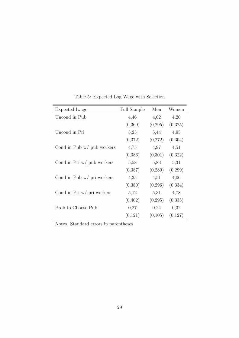
Table 5: Expected Log Wage with Selection

Expected lwage Full Sample Men Women

Uncond in Pub 4,46 4,62 4,20

(0,369) (0,295) (0,325)

Uncond in Pri 5,25 5,44 4,95

(0,372) (0,272) (0,304)

Cond in Pub w/ pub workers 4,75 4,97 4,51

(0,386) (0,301) (0,322)

Cond in Pri w/ pub workers 5,58 5,83 5,31

(0,387) (0,280) (0,299)

Cond in Pub w/ pri workers 4,35 4,51 4,06

(0,380) (0,296) (0,334)

Cond in Pri w/ pri workers 5,12 5,31 4,78

(0,402) (0,295) (0,335)

Prob to Choose Pub 0,27 0,24 0,32

(0,121) (0,105) (0,127)

Notes. Standard errors in parentheses

29

Appendix

Wage Decomposition with Sectoral Choice

E(w|RA,Pu, f = 0)−E(w|RA,Pu, f = 1) : Normal Wage Equation Controlling for RA, Gender, and Sector

= Pr(Pu = 1|RA, f = 0)E(w|RA,Pu = 1, f = 0)+(1−Pr(Pu = 1|RA, f = 0))E(w|RA,Pu = 0, f = 0)

−Pr(Pu = 1|RA, f = 1)E(w|RA,Pu = 1, f = 1)−(1−Pr(Pu = 1|RA, f = 1))E(w|RA,Pu = 0, f = 1)

= Pr(Pu = 1|RA, f = 0)[E(w|RA,Pu = 1, f = 0)− E(w|RA,Pu = 0, f = 0)]

−Pr(Pu = 1|RA, f = 1)[E(w|RA,Pu = 1, f = 1)− E(w|RA,Pu = 0, f = 1)]

+[E(w|RA,Pu = 0, f = 0)− E(w|RA,Pu = 0, f = 1)] : Wage Gap in the Private Sector

= Pr(Pu = 1|RA, f = 0)E(w|RA,Pu = 1, f = 0)−Pr(Pu = 1|RA, f = 0)E(w|RA,Pu = 0, f = 0)

[+Pr(Pu = 1|RA, f = 0)E(w|RA,Pu = 1, f = 1)−Pr(Pu = 1|RA, f = 0)E(w|RA,Pu = 1, f = 1)]

−Pr(Pu = 1|RA, f = 1)E(w|RA,Pu = 1, f = 1)+Pr(Pu = 1|RA, f = 1)E(w|RA,Pu = 0, f = 1)

[+Pr(Pu = 1|RA, f = 0)E(w|RA,Pu = 0, f = 1)−Pr(Pu = 1|RA, f = 0)E(w|RA,Pu = 0, f = 1)]

+[E(w|RA,Pu = 0, f = 0)− E(w|RA,Pu = 0, f = 1)]

= Pr(Pu = 1|RA, f = 0)[E(w|RA,Pu = 1, f = 0)− E(w|RA,Pu = 1, f = 1)]

−Pr(Pu = 1|RA, f = 0)[E(w|RA,Pu = 0, f = 0)− E(w|RA,Pu = 0, f = 1)]

+[Pr(Pu = 1|RA, f = 0)− Pr(Pu = 1|RA, f = 1)]E(w|RA,Pu = 1, f = 1)

−[Pr(Pu = 1|RA, f = 0)− Pr(Pu = 1|RA, f = 1)]E(w|RA,Pu = 0, f = 1)

+[E(w|RA,Pu = 0, f = 0)− E(w|RA,Pu = 0, f = 1)]

= Pr(Pu = 1|RA, f = 0)[[E(w|RA,Pu = 1, f = 0)− E(w|RA,Pu = 1, f = 1)]

−[E(w|RA,Pu = 0, f = 0)− E(w|RA,Pu = 0, f = 1)]

+(Pr(Pu = 1|RA, f = 0)−Pr(Pu = 1|RA, f = 1))[E(w|RA,Pu = 1, f = 1)−E(w|RA,Pu = 0, f = 1)]

+[E(w|RA,Pu = 0, f = 0)− E(w|RA,Pu = 0, f = 1)]

= Pr(Pu = 1|RA, f = 0)[E(w|RA,Pu = 1, f = 0)− E(w|RA,Pu = 1, f = 1)

+(1− Pr(Pu = 1|RA, f = 0))[E(w|RA,Pu = 0, f = 0)− E(w|RA,Pu = 0, f = 1)

+(Pr(Pu = 1|RA, f = 0)−Pr(Pu = 1|RA, f = 1))[E(wf |RA,Pu = 1)−E(wf |RA,Pu = 0)] : positive term

Therefore, when we observe the wage gap conditional on sector and risk aversion (RA, Pu),

we overestimate the gap with the additional positive term (Pm−Pf )[E(wf |Pu = 1)−E(wf |Pu =

0)], which reflects the selection preference.

30