Embed Size (px)
Citation preview

Progress in Nuclear Energy, Vol. 18, No. 1/2, pp. 237-250, 1986. 0149 1970/86 $0.00+.50 Printed in Great Britain. All rights reserved. Copyright © 1986 Pergamon Journals Ltd.
THE FINITE ELEMENT RESPONSE MATRIX METHOD FOR THE SOLUTION OF THE NEUTRON TRANSPORT EQUATION
JAMES A. RATHKOPF* and WILLIAM R. M A R T I N
Department of Nuclear Engineering, The University of Michigan, Ann Arbor, Michigan, U.S.A.
Abstract--The finite element response matrix method has been applied to the solution of the neutron transport equation. This method has previously been applied to the neutron diffusion equation for coarse mesh reactor analysis with excellent results. As with the diffusion equation implementation, the transport method employs a local-global projection technique to allow treatment of internal heterogeneities that would normally not be resolved by the coarse global mesh that is needed for computational efficiency. However, since the transport equation includes the angular domain, the local~lobal projection technique has been extended to angle as well as space. Since the response matrices do not depend on the multiplication factor, a conventional fission source iteration method is utilized for criticality problems. The method has been applied to the one-dimensional and two- dimensional neutron transport equations. For one-dimensional geometries, the local global projection method yields excellent results, indicating the potential of this approach as a viable coarse mesh transport method. Numerical results are presented for several one-dimensional configurations that were analyzed with varying choices of local and global meshes in the spatial domain. Preliminary results with two-dimensional applications indicate that computational times may be an order of magnitude faster than with the conventional finite element solution of the two-dimensional transport equation.
1. INTRODUCTION
The development of the application of the finite element method to the neutron transport equation may be divided into two approaches: variational methods applied to the second-order form of the neutron transport equation and weighted residual methods applied to the conventional first-order equa- tion. Early work with the second order form dealt with finding a solution on the complete phase space domain. 9"I° Later efforts partitioned the spatial domain into smaller regions and recast the method into a response matrix or interface current approach. 2'3 Work on the first-order form has pro- ceeded in a similar fashion. One- and two-dimensional applications 7'16 demonstrated the success of the conventional finite element method. Subsequent effort 5'6's employed a partitioning (or segmentation) of the spatial domain into sub-regions with a global iteration technique coupling the sub-regions together, achieving a significant increase in computational efficiency. This approach has many similarities to an interface current approach, although would not be classified as a response matrix method.
In this paper we present the development of a response matrix formulation of the finite element
* All correspondence to: Nuclear Fuel Division, West- inghouse Electric Corporation, Pittsburgh, PA 15230, U.S.A.
237
method applied to the first-order form of the transport equation. The inspiration for this approach is a finite element response matrix method applied to the neutron diffusion equation. 12 As in that work, two levels of polynomial expansions (i.e. with finite element basis functions) are used. One, the local level, is defined on a mesh fine enough to provide reasonable accuracy. The second, the global level, is a coarser mesh which reduces computational effort. The methodology for linking the local and global calculations is a key aspect of the overall method.
In Section 2, we present the basics of the response matrix formulation in which the conventional re- sponse matrix is divided into two matrices in order to remove the dependence of the response matrix on the multiplication constant. A typical mesh (either global or local) is described in Section 3, and response matrices are developed by expansion of fluxes and sources in terms of finite element basis functions defined on the given mesh. In Section 4, the finite element method is applied to the first-order neutron transport equation on the local mesh, obtaining the local response matrices. Then, by projecting the local solution onto the global mesh, global response matrices are defined. The results of application of the response matrix method to several one-dimensional benchmark problems are discussed in Section 5. Conclusions are drawn in Section 6, and the

238 J.A. RATHKOPF and W. R. MARTIN
application to two-dimensional geometries is briefly discussed.
2. RESPONSE KERNEL EQUATIONS In this section, the alternative formulation of the
response matrix method is modified from that pre- sented by Nakata and Martin ~2 to allow application to the transport equation rather than the diffusion equation. Here, response kernels are defined rather than response matrices. In Section 3, the spatial and angular dependence is discretized to obtain response matrix equations that approximate the response kernel equations.
The spatial domain ~ upon which a solution of the neutron transport equation is desired is divided into L regions, denoted by ~t, such that
L ~ = U ~t"
I - 1
The following notation will be used throughout the formulation:
tg~ = boundary of region l
V~ = phase-space: ~ x 4n
n, = unit outward normal to t3~'t
F~ = t g ~ x 4 n
F~ + = outgoing boundary: all (r, It)eF, for n~. I t > 0
F~- = incoming boundary: all (r, It)~F~ for n~' I t<0 . Consider the first-order neutron transport equation
for a single region ~,
1~ • V~b(r, f t ) + ~,(r)~(r, 11)
= / dit'~C~(r, I t " It)~b(r, It') 34 / t
+ S(r, f~) for (r, It)e V~
subject to a specified incoming boundary condition
~b(r. It) = ~bi,.l(r, It) on r [ .
The source S(r, [1) includes production of neutrons due to fission or an external source. Solution of this equation will yield the spatial and angular distribution of neutrons on V~ and the outgoing angular flux ~bl+(r, It) on the outgoing boundary Fz +.
Because the transport equation is linear, a response kernel equation may be written to relate tb~÷(r, tl), $in3(r, It), and S(r, It)
~z+(r, It) = f ds' dfl'ln ~ • It'l dr
Rsl(r ', ~'--.r, It)~bi,3(r', It')
+ .Iv, dr' d~'R~v
(r', I t ' ~ r , It)S(r', It') for (r, It)~Fl +
(1) where
Rs t (r', It'--* r, It) = response kernel for outgoing angular flux due to the transport of the neutrons entering region l
Rvt(r ', I t ' ~ r , It) = response kernel for outgoing angular flux due to the transport of the neutrons produced within
In the conventional response matrix formulation, this expression would take the form
~bl+(r, ~) = f ds' dit'ln ~ • It'lg'(r', I t ~ r , It) dr
~bin,l(r' , It') e x l + ~b~+(r, f~) for (r, It)~F~ + (2)
where
R~(r ', I t ' ~ r , It) = response kernel for outgoing angular flux due to an arbitrary incoming flux
~b~. t = outgoing angular flux due to fixed source within ~ r
The alternative formulation divides the conventio- hal response kernel R ~ into two parts, R~ and R~, representing surface-to-surface and volume-to-volume transport of neutrons, respectively. This partitioning is similar to that used in interface current methods and collision probability methods.
The angular flux ~b(r, It) on the region interior can also be expressed in terms of the incoming flux and source:
q~(r, It) = ~ ds' dit'ln z • It'lM~ dr
(r', I t ' ~ r , It)~bin3(r', ~')
+ f dr' , t , di t My(r , It'--*r, It)S(r', f~') Jr,
for (r, It)~V I. (3)
The kernels M~(r', It '-*r, It) and M~.(r', It '-*r, It) represent the surface-to-volume and volume-to- volume transport of neutrons, respectively.
A region coupling equation can be written by defining Him(r', It '-*r, It) for (r', It ')eF +, (r, It)eF I- 1, m = 1 . . . . . L, as the probability that a neutron leaving region ~m at r' with angle I t ' will enter region ~ at r

The FEM response matrix method 239
with angle f~. Because the regions are assumed to be contiguous, H~, represents the continuity of neutron flow across an interface and serves as a reindexing scheme to identitify neighboring nodes:
¢~in.t( r' ~"~) = E ds' df l 'H, , . m = l ,~
(r', fV--,r, f~)4~.+(r', fg)
for (r, f~)eF/. (4)
If the response kernels were known, these three kernel equations (1), (3) and (4) could be used to find the angular flux distribution on ~. Unfortunately, they are not known. In the following section, the response kernel equations will be recast into response matrix equations, which will be solved by the finite element method.
3. RESPONSE MATRIX EQUATIONS
Approximate forms of the response kernels can be found by approximating the spatial and angular dependent fluxes and source by expansions in terms of polynomials. These expansions in effect discretize the phase space of each region. The result of this discretization is the set of response matrix equations.
Let region ~ contain N spatial points on its interior and N s spatial points on its boundary 0~ . Further- more, define K points on the angular domain. The phase space V~ therefore contains M = NK points and the phase space boundary F t contains M s = N s K points. Define polynomials q~,(r, fl), i= 1 , . . . , M, which have value one at point i and zero at the remaining interior phase space points, and poly- nomials qJsff, 1)), j = l . . . . . M s, which have value one at point j and zero at the remaining boundary phase space points.
On each regions ~'~ the incoming and outgoing fluxes and the volume flux and source can be expanded in terms of the appropriate polynomials:
Ms t~in.l(r' ~'~) = E Vs,(r, ~"~)~bisn./j (5a)
j - - I
Ms ~bt+(r, l'/) = ~ Vs,(r, n)q~s+j (5b)
j = l
M
~b(r, a ) = ~ q~i(r, fl)tb, v (5c) i = 1
M
S(r, n ) = ~ q~,(r, n ) S [ (5d) i = 1
where s s v v qSt+~, and are the expansion ~ i n . l j ' (~ll all
coefficients. The superscripts S and V indicate expan- sion coefficients in surface and volume polynomials, respectively.
The vector notation
T(r, f~)=col(hUl(r, f~), q~2(r, f~) . . . . qJu(r, ~))
• s(r, fl)=col(Wsl(r, f~), qJs2(r, fl) . . . . . q~sMJr, f~))
01s .t = col($S ,,,, s s (~in,/2~ ' s
el+ = col(4,L 1, 4~L 2, . . . . 4'f+ M)
v colt,6v ,6v , ~bv)
s~ = co l (SL s,~ . . . . . s,~)
allows less cumbersome expressions for the expansions
qSi.a(r, f~) r s =Tsbi . , l (6a) ~bt+(r , f~)_ r s - T s b, + (6b)
~b(r, fl) = V r b v (6c)
S(r, f~) ='I'TS, ~ (6d)
where T indicates transpose. Substitution of these approximations into response
kernel equations (1), (3) and (4) and application of the Galerkin weighted residual technique yields the re- sponse matrix equations. In particular, the outgoing angular flux is found by multiplying equation (I) by Vs,(r, ~) and integrating over the outgoing surface F~ + yielding
S 1 S 1 v bl + = Rs~ sbin,, + Rs~v S~ (Ta)
Equation (3) is weighted by qJff, fl) and integrated over V t to get
b V : M ~ s b ~ . , t + M ~ v S , v (7b)
The continuity matrix equation is found by integrating equation (4) with the weighting function q~sj(r, l'~) over the incoming surface F [ :
L I~iS, E H , , . s = b,.+- (7c)
m = l
The response matrices in the three preceding equations are easily obtained by formally inverting the matrix equations that arise when the Galerkin weighted residual method is applied.
Matrix equations for each region can be combined to form a set of equations (and an iterative solution scheme) for the entire spatial domain ~ by defining
S S S S ) b i n : c o l ( b i n , l ' ([)in,2 . . . . . b i n , L
b s = col(bS +, bs2 + . . . . s , ¢~+)
b ~ = co~lb~, b~ . . . . . b D
SV=col(S~, S v . . . . . Sff).

240 J.A. RATHKOPF and W. R. MARTIN
The individual regional response matrices are also combined to form large block diagonal matrices, resulting in the following iteration scheme
d#stn)_ l~ ,kStn- ~).a_ l~ SVtm- ~) + - - ~ S ~ S ~ " i n ~ ~ S ~ V
~ S ( n ) - l . l d ~ S ( n )
~ ) V ( m ) - - 111/i ~KS(n) -1- ~b l . ~ V ( m - 1 ) . . . . V ~ S , V f i n t . . . V ~ V O (8 )
where n is the inner iteration index (to converge on the interface flux distribution) and, in the case of a critical eigenvalue problem, m is the outer iteration index. The source term is written
1 S v t - I = k(,,,) Fd~ et ' ) (9)
where F is the usual fission production term and k is the multiplication factor. This method of solution is the conventional inner-outer source iteration scheme. If the system contains no fissile material, the external source is specified and the global distribution of neutrons is found by iterating only on the interface fluxes.
for which a solution is desired on region ~ subject to an arbitrary neutron source and irradiation on the surface F f
(~(r , l '~) = ~bin,,(r , ~'~) o n I- ' t - . (11)
The solution is found by applying the finite element method not to this equation itself but to an equivalent weak form which is found by multiplying equation (10) by ~b~(r, f~), an element of the function space H~ (or 'energy' space) defined by
where
(q~, ~b)~ = local volume inner product
- ~ S dr dl~b(r, fl)g,((r, fl). ,jr i
The solution itself, ~(r, fl), is assumed to be a member of this function space. After integration by parts, the desired weak form of the transport equation is obtained for region l:
Find ~(r, fl)eH~, such that for all ~(r, ~)e//~
4. RESPONSE MATRICES FROM THE FINITE ELEMENT METHOD
The response matrix equations and a solution method were developed in Sections 2 and 3 under the assumption that the response kernels themselves were known. Generally, this is not, of course, the case. Fortunately, the response matrices can be found directly from the first-order neutron transport equa- tion by application of the finite element method to find a solution on each spatial region. In order to obtain a suitably accurate solution the phase space domain is divided into a fine 'local' mesh. Then, to reduce the computational effort required to solve the response matrix equations iteratively, this local solution is projected onto a coarser 'global' grid resulting in the response matrix equations presented in Section 3.
In Section 4.1, the local response matrices will be developed directly from the transport equation. Then, the global response matrices will be found via a weighted projection technique in Section 4.2.
4.1. Loca l response matr ices
Now return to the first-order form of the neutron transport equation
~ " VO(r, ~ ) + E,(r)O(r, ~)
= f d~'Es(r, ~ ' - l~)~b(r, ~ ' )+S(r , l'~), (10) n
=(Ks¢,t~b, ~b,),+(S, ~b,), (12)
where
(q~, ~b) ±l = local surface inner product
~- [ ds drain t • ~l~b(r, ~)~(r, g~) Jr
and the scattering operator is defined
Kscatq~(r, [~) -= f,,~ df~'Es(r, f~" l~)~b(r, fl'). (13)
In order to reduce the infinite number of trial functions ~bt(r, fl) to a manageable amount, a finite- dimensional subspace of H~ is defined. This subspace, S~, is constructed by defining N~ interior spatial points in the region ~t~ and Kt angular points such that M~ = NzK t is the total number of phase space support points. The superscript h provides a measure of the spacing of these phase space points. The points identify the elements of S~ which are piecewise polynomials ~,u(r, fl), i= 1 , . . . , M~, that are unity at phase space point i and zero elsewhere. Because the solution ~b(r, fl) assumed to be a member of S h, it can be expanded in terms of the basis functions ~,li(r, ~)
M t qS(r, ~ ) = ~ ~ku(r , ~)qSu=dffdp~ v (14)
i = 1

The FEM response matrix method 241
where
~ , = c o l ( q r , ~ , 2 . . . . . ¢i~,) IV - - IV IV IV ~I -col(Si1, St2, , • . . S l ~ ) .
The superscript l V denotes coefficients of expansion in the local volume space. Requiring the weak form to be satisfied for all ~ij, j = 1 . . . . . Mi, results in the matrix equation
AI¢II V = Oin,I "F S! (15)
where
A,~, = - ( q , ii ,f~ Vq6)i + <~'i i , ~ ' l i> +i
- ( K ~ . , q , . , q'ij)I + (X,¢., q'lj)i
and the contributions of the incoming flux and source a r e
d~n,, = f ds dftln I • nlSi.,t(r, n)~i(r, ft) dr f
~-- <b in , l , ~ / I ) - l ( 1 6 a )
SI = ~ S dr d.qS(r, f~)~z(r, f~) dr i
= (S, ~t)l- (16b)
Because As is nonsingular, it can be inverted to obtain an expression that gives the angular flux on the interior of ~l from the contributions of the incoming angular flux at the region boundary and those of the arbitrary neutron source:
t ~ t = A I- l t~ in , t+ A t - I s I. (17)
The outgoing surface flux Sl+(r, 11) can be expanded in terms of surface basis functions ~01sff, f~ ), j = 1 . . . . . MIS, which are defined only on the bound- ary F I. The boundary contains Nis spatial points. The polynomials have value one at phase space point j, zero elsewhere. The total number of local surface support points is Mis = NIsK l. The resultant expansion is
Sl+(r, r IS 1"~) = ~ l ~ , + (18)
where
lilts = COI(~,bISI' ~ lS2 . . . . . I~l tSM,s)
d~,l s = col(Sift+l, IS is S 1 + 2 ' " ' " " SI+MIs)"
The outgoing flux is simply the angular flux on the outgoing boundary F~+:
S,+(r, f t)=S(r, fl) (r, ft)~F 7.
Substitute into this equation the expansion for S(r, f~), S(r, n) = O/SdOll v (19)
and that of Sl+(r, fl) (equation (18)) and apply the Galerkin weighted residual method to obtain
IS IV T~s,IsqI + = TIs,IOn (20)
where T
Tts,ts = < OllS,O/zs> +l (21 a)
T, . r IS l = <OlS, ~t > + I" (21 b)
Equation (20) expresses the relationship between the two expressions for the angular flux on the outgoing boundary: expanded in terms of the interior basis functions and expanded in terms of the boundary basis functions. Formally solve equation (20) for dpff,
IS T-1 T a~w (22) ~ l+ ~ ~ IS,IS ~lS,f"gl
and substitute into equation (17) to find the outgoing flux in terms of the incoming angular flux and source,
O[S+ = Rls,l~Oin. ! + Rts, tS l (23)
where
Rts, ̀ = i t s ) s T~s,IA I- 1. (24)
The matrix Rls,i is, in a sense, a local response matrix. It will become part of a true response matrix once the contribution Oi.,l is related to the expansion coefficient
In order to find the flux distribution over the entire space domain ~, the individual regions must be coupled via a coupling equation. Assuming conti- guous nodes, continuity of neutron flux across region interfaces mandates for adjacent regions ~l and ~,,
Sin,i(r, £"~)=~m+(r, ['~) for (r, fl)eF~ (25)
where F~ is that part of F t- that coincides with part of F +. Substitute the expansions for S=+(r, fl) and Sin,l(r , ~'-~ ),
S.+(r, r ,.s ~ ) = ~mS~m + (26a)
Sin.t(r, r IS 1-~) = Otsd~in,t (26b)
and apply the weighted residual method to obtain
L Tts,lsd#Is,, = X HIs,msd~,.ms+ (27)
m = l
where lt~s,,.s is a matrix similar to T~s,I s in that it consists of terms of the form <qrs,$.,s> +l. The terms, however, are arranged in such a way as to indicate which regions are adjacent and which direction neutrons must flow in order to leave one region and enter its neighbour. The more familiar continuity matrix equation results by multiplying equation (27) by T- 1 and redefining//~s ,.s: IS,IS
L IS ¢in. l = Y~ . .s His,.,sd#., + . (28)
m = l

242 J.A. RATHKOPF and W. R. MARTIN
All that remains to generate a set of local response matrix equations is the reconciliation of d~.t and ~'~.v
We rewrite equation (16a) to serve as a reminder that the contribution of the incoming surface flux to the finite element equation is a simple inner product:
Illin,t = <q~in.t( r, [~), OA r, f ~ ) ) - v
Substitute the polynomial expansion for the incoming surface flux,
~bin,/(r ' T ts l-l) = 0t~lh..t (29)
into equation (16a) to obtain the relationship
¢in,/-~- rl,lst~liSn,l (30)
where
T~,,s = (Or, o r > -v (31)
Substitute equation (29) into equation (23) and define
Rts,ts = Rts,~ T~,ts
- T - t Tt s tA t- t Z (32) -- IS,IS , l,lS
and
Mt.t s =A t- 1Tl.i s (33)
to obtain the system of local response matrix equa- tions:
IS _ R~ S IS 1 ~l + -- ,lSl~in.I + RIs,ISI
dptis t = ~ Hzs,,.sdp: s ~ (34)
*ttv= ml,tS(llliSn,i.-~- a l - l Sl. J
Equations (34) represent the finite element solu- tion to the transport equation on the regions ~t, 1= 1 . . . . , L. They could be used in an iteration scheme such as equation (8) to find the particle distribution over the entire phase space V. This might be computationally expensive, however, due to the fine local mesh. By projecting the solution onto a coarser global mesh, computational requirements can be reduced. In the following section, global response matrices are constructed from the local response matrices developed here.
4.2. Global response matrices
The global response matrices are found from the local response matrices by reconciling the local polynomial expansion approximations presented in the previous section with the global polynomial expansions of Section 3, equation (6). The already well-used Galerkin weighted residual technique serves as the tool of reconciliation.
Equations (6b) and (6c)--the global polynomial expansions for the outgoing flux ~bt+(r, fl) and the region interior flux ~b(r, f~)--are rewritten here:
~t +(r, n ) = v ~ 0 f +
¢(r, n ) = v r * v.
The global approximations cannot simply be equated to the local approximations given in equation (15) and (14). However, they can be made equal in a weighted residual sense by requiring the residuals to be ortho- gonal to ~s and T, respectively:
Tss~S+ = Ts.tsdptt s (35a) V IV rvvd h - rv. f lh (35b)
where
Tss = (Uls, ' e r ) +t
T Tsas = ( T s , dlts) +l
Ttvv =(T, Tr),
Tv., = ('r, 0[),.
Substitute equations (35) into the response matrix equations given in equations (34) to obtain
Os+ = r ~ 1 rs.,s(R,s,,¢in., + gts.,S,)
d# v = Tvv t Tv.t(A t- ld~in,, + A t- tSt). (36)
The contributions O~,.t, once again, and S t can be related to the global expansion coefficients by recalling equations (16)
{~in,/~" (~bin.t(r, f~), 0t( r, f l ) ) - t
S t = (S(r, f~), 0t(r, f~))v
Substitute equations (6a) and (6b),
Sa) - ~I' s ¢ i . , t 4'i.,,(r, _ • s
S(r, ~ ) = 'I' r S v
into equation (16) and evaluate the surface and volume inner products to obtain
~in,t = Tl,Sl~Sn,t (37a)
S t = Tt.vSt v (37b)
where
and
r~s = ( ' l ' s , 0 [ > - ,
r,.v = ( v , 0/) , .
Substitute equations (37) into equation (36) and define
R z s,- s = Tss t Ts,lsRls a TI,s (38a)
R ~ . v = r i s 1Ts.,sR,s.,TLv (38b)

The FEM response matrix method 243
M~ us = r f d rv,tA,- 1 Tz.s (38c)
1 - - - 1 - 1 M v ~ v - T(, v Tv.tA t T~, v (38d)
to obtain the long sought after global response matrix equations:
S 1 S 1 V dPt ÷ = Rs , - s ¢bi~,t + R s ~ v St
V t S t V d~t = M v ~ s ~i.,l + M v ~ v St •
Thus the finite element method has been used in conjunction with a local-global projection technique to generate the response matrix equations which are identical to the formal equations derived earlier as equations (7).
5. NUMERICAL RESULTS
The finite element response matrix method for solution of the transport equation has been formulated for both one- and two-dimensional applications. In this paper, however, only the one-dimensional, application will be discussed because additional work is necessary to further improve upon the two-dimen- sional results.
In one dimension the spatial domain is divided into regions whose boundaries usually fall on material interfaces. On each region a local mesh and a global mesh of points are specified which define the Lagrangian polynomials that are used in the poly- nomial expansions described in Section 4. Similarly, two sets of mesh points are specified on the angular domain, denoted by the cosine p. Lagrangian poly- nomials are again used as the basis functions. The multi-dimensional (x, #) polynomials are found by taking the tensor product of the space and angle polynomials. Because no spatial variation can exist along the boundary of one-dimensional regions, the expansions of incoming and outgoing surface fluxes are in terms of Lagrangian polynomials defined in the angular domain, not both the angular and spatial domain.
It has been found in other applications of the finite element method to the first-order form of the transport equation 7 that significantly improved results are obtained if discontinuities in the neutron angular flux are allowed at points in the angular domain that distinguish outgoing neutrons from incoming neu- trons. In one-dimensional plane geometry this point corresponds to/~ = 0. This discontinuity is handled by supplying two angular support points at # = 0 instead of only one.
Once the multi-dimensional local and global, volume and boundary polynomials have been defined, the finite element matrix A t is found for each unique
region by evaluating the various integrals included in the definitions of its matrix elements. Because the phase space polynomials are tensor products of individual one-dimensional polynomials, the multi- dimensional integrals are also tensor products of one- dimensional integrals. The matrix is inverted by means of LU-decomposition. The size of A t is small because only a small fraction of the entire spatial domain is included in A t thereby allowing the inversion to be reasonably inexpensive.
The various projection matrices, denoted by T earlier, are also the tensor products of one-dimen- sional matrices found by evaluating inner products. Furthermore, the inverse of the multi-dimensional matrices are simply the tensor products of the inverses of the one-dimensional matrices. This fact further reduces the cost of generating the response matrices.
The resultant surface-to-surface response matrix, Rs ~s, has a form which lends itself to iterative solution by the Gauss-Seidel method and, by extension, the successive over-relaxation (SOR) method. The con- verged fluxes are found using SOR and alternating the sweep between left-to-right and right-to-left. No acceleration schemes have been attempted in the outer, source iterations that are necessary for the solution of eigenvalue problems.
Three different one-dimensional test problems were analyzed as a means of evaluating the finite element response matrix method: two of these problems-- Reed's problem and Alcouffe's problem--contain strong heterogeneities; the third problem is actually a series of homogeneous eigenvalue problems.
5.t. Reed's problem
Reed's problem, x5 as depicted in Fig. 1, was originally devised to test differencing schemes for discrete ordinates codes. It is a problem of four different material regions with a non-uniform, iso- tropic source distribution, a reflecting boundary condition on the left, and a vacuum boundary condition on the right.
Figure 2 is a plot of the scalar flux distribution in Reed's problem obtained with the Monte Carlo code TART, 13 which shall be considered a benchmark solution. The obvious features of this profile include a peak at the source zone of the scattering material, a plateau in the void due to neutrons travelling from the scatterer on the right to the gray and black regions on the left, a depression to nearly zero in the sourceless gray region as the neutrons traveling left are absorbed, and another plateau of value 1.0 in the intensely absorbing region with the large source. The flux distribution in both the void and gray region is due to

244 J.A. RATHKOPF and W. R. MARTIN
tell.
reg.l
S=50
Zt=50
Zs=O
I 0
reg. 2
S=O
~t=5
Zs=O
reg.3
S=O
Zt=O
Zs=O
I 4
x (cm)
(units: Zt, Zs,
reg. 4
S=1 i I 2t=l. i
ZS=.91
S [cm-l])
Fig. 1. Reed's problem.
reg. 5
S=O
~t=l.
Zs=.9
I
vac.
oi
X -I o
0 0 o o
Reed's P r o b l e m - - S c a l e r Flux Y TART
V~VVVY~~YVVVYYYV~
o ,q 0 I 0.00 1100 2'.00 3'.00 4'.00 5.00 6'.00 7'.00 8.00
×(cm) Fig. 2. Reed's problem: Monte Carlo benchmark.
neutrons from the scattering source. The flux, there- fore, is extremely anisotropic throughout the problem, except in the black absorbing region, where the source itself forces isotropy, and the scattering region.
Reed's problem has been analyzed using FTRAN, 7 a conventional one-dimensional finite element code, and using the response matrix method with a variety of local and global spatial mesh spacings. In all cases both the local and global angular domains
contain six support points located at p = - l , -0 .5 , - 0 , +0, +0.5, + l. Thus there was no attempt to utilize a local-global projection in angle for this test problem.
Figure 3 depicts the scalar flux found by three different applications of the response matrix method. The profile labelled 5/5/cm indicates a calculation in which both the local and global mesh contains five mesh points per cm, corresponding to a uniform mesh

Reed's P r o b l e m - - S c o l o r Flux
"1 5 / 5 / cm x 5 / 3 / cm
o
d
The FEM response matrix method 245
! !
,ioo 2'.0o 3'.oo ,.oo i oo 6.00 ¢.oo ×(cm)
Fig. 3. Reed's problem: response matrix (mesh size=0.5 and 0.25 cm).
o
o
IO.00 8.00
spacing of 0.25 cm. Each response matr ix region spans 1 cm. Al though not plot ted in this figure, the F T R A N results using the same 0.25 cm mesh coincide nearly exactly with the 5/5 response matr ix values. Both agree quite well with the M o n t e Car lo benchmark as can be seen from the errors listed in Table 1. The errors listed in Table 1 and succeeding tables of this type are defined
f :~ [~brer(x ) - qS(x)] dx
relative error = - "
and
Ei? ] [~,e: ( x ) - ~(x)] 2 dx ~ RMS error = "
[q~r,f(x)] 2 dx ~ a
where qS,cf(x ) is the reference scalar flux {TART), #~(x) is the scalar flux in question, and x a and x b are region boundaries . The flux is assumed to vary linearly between the points plot ted in Fig. 2. The regions of Table 1 are the mater ial regions as numbered in Fig. 1.
Also plot ted in Fig. 3 are the profiles of two cases in
Table 1. Errors in scalar flux for reed's problem (errors with respect to Monte Carlo benchmark; angular support points: 6; response matrix convergence criteria: 10-5)
Error
Region
Case Total 1 2 3 4 5
Relative error (%) FTRAN a 0.069 -0.002 -3.312 0.039 0.722 -0.216 5/5 b 0.069 -0.002 -3.311 0.039 0.723 -0.216 5/3 0.055 -0.024 -6.142 0.038 0.953 -0.294 3/3 0.274 -0.025 -5.524 0.621 1.061 -0.243
R M S error (%) FTRAN 1.169 0.434 8.522 0.039 1.556 0.789 5/5 1.169 0.434 8.522 0.035 1.556 0.788 5/3 2.860 0.483 29.17 0.038 3.128 1.424 3/3 3.317 0.468 26.21 0.621 4.414 1.672
a FTRAN mesh structure: five support points/cm. b 5/3 indicates Response Matrix mesh structure of five local support
support points/cm. points/cm and three global

246 J.A. RATHKOPF and W. R. MARTIN
which the global mesh is 0.5 cm (cases 5/3 and 3/3). The local mesh size, however, is 0.25 cm for 5/3 and 0.5 for 3/3, i.e. for case 5/3 fine mesh response matrices are projected onto a coarser global mesh. The RMS errors presented in Table 1 demonstrate that although both the coarse mesh solutions provide less agreement with the benchmark than the fine mesh solution (especially in the gray region, 2, although the percent errors here are misleading because the flux itself is nearly zero), the 5/3 solution is in better agreement than the 3/3 solution in the void and region 4, the source-scattering region. Projecting the response matrices from a fine mesh, therefore, improves the results of a coarse mesh calculation.
To further demonstrate the local-global projection method, a series of coarse mesh calculations with a spacing of 1.0 cm were performed, as listed in Table 2. In all of the response matrix calculations, a global mesh of 2 support points per cm is used with each response matrix region spanning 1 cm. The local mesh, however, varies from a fine mesh of 5/cm to coarser meshes of 3/cm and 2/cm. For the 2/2 case, where the local and global meshes are the same, the results are nearly identical to those of the FTRAN calculation performed with the same 1 cm mesh spacing. With decreased local mesh size, however, better agreement is seen with the benchmark, even though the same coarse global mesh is used throughout. The overall improvement is not dramatic but in several regions--the void, in particular, and region 4--i t is significant.
Additional calculations 14 have shown that results
obtained by the response matrix method are indepen- dent of the size of the response matrix region if the mesh spacing is held constant. Furthermore, increased accuracy may be obtained by using polynomials of higher order. In all the cases presented above linear polynomials were used.
Computational times required by the Amdahl 5860 computer at The University of Michigan to solve Reed's problem are presented in Table 3. The compu- tational costs can be divided into two components: the cost of generating one or more response matrix sets and the cost of the iteration solution procedure itself.
The response matrix generation cost is dependent on the local and global mesh size desired and whether the two mesh structures are identical. The costs, of course, increase with the number of support points. If, however, the global mesh is identical to the local mesh, the costs are somewhat reduced because some calcula- tions may be bypassed.
The cost of finding the global solution is dependent on a number of factors, including the number of iterations required to reach convergence and the cost per iteration. The iteration count depends on the number of regions in the problem, the physical characteristics of the problem, and the iteration scheme chosen.
For most of the solutions to Reed's problem, the iteration costs are much less than the cost of generating response matrices, as seen from Table 3. The only exception is the 32 region problem. For that case the response matrix generation costs are less because the regions contain few support points. The iteration costs
Table 2. Errors in scalar flux for coarse mesh Reed's problem: constant global mesh (errors with respect to Monte Carlo benchmark; angular support points: 6; response matrix convergence
criteria: 10- ~)
Error
Region
Case Total 1 2 3 4 5
Relative error (%) FTRAN a -2.190 -0.046 8.132 -2.104 -5.918 --1.700 2/2 b -2.104 -0.055 8.133 -2.126 -5.958 - 1.176 3/2 0.252 -0.004 --0.249 -0.621 0.334 -0.011 5/2 0.071 -0.004 --0.064 -0.038 0.342 -0.101
R M S error (%) FTRAN 7.392 0.604 60.39 2.104 9.579 3.783 2/2 7.349 0. 569 60. 39 2.126 9.603 3.030 3/2 6.322 0.557 60.04 0.621 7.565 2.685 5/2 6.313 0.556 60.03 0.038 7.565 2.691
a FTRAN mesh structure: two support points/cm. b 3/2 indicates Response Matrix mesh structure of three local support points/cm and two global
support points/cm.
The FEM response matrix method
Table 3. Computational costs to solve Reed's problem (AMDAHL 5860)
247
Mesh structure
Local Global
Total Iteration response
Number matrix Total of generation Total CPU CPU
regions time (sec) inners time (sec) time (sec)
33 ' 5 5
5 3 3 3
9,5 9,5 2 2
9 "'2 2
3 2 5 2
. . . . . . . . . . . 0.065 a 0.196 ' i3 0.016 0.212
8 0.220 13 0.011 0.231 8 0.128 13 0.012 0.140
5 0.443 14 0.019 0.462 32 0.108 59 0.115 0.223
. . . . . . . . . . . . 0.017 a 0.108 i ; 0.009 0.117
8 0.128 13 0.012 0.140 8 0.200 13 0.011 0.211
aFTRAN.
are high because the many regions cause an increase in both the effort required for each iteration and the iteration count.
The F T R A N times quoted in Table 3 indicate that the response matrix method is not competitive with F T R A N for this type of problem. This is a conse- quence of the explicit inversion necessary to generate response matrices. F T R A N solves the finite element matrix directly (but does not invert it) while taking advantage of its band structure. This results in a linear
dependence of costs to the number of spatial mesh points.
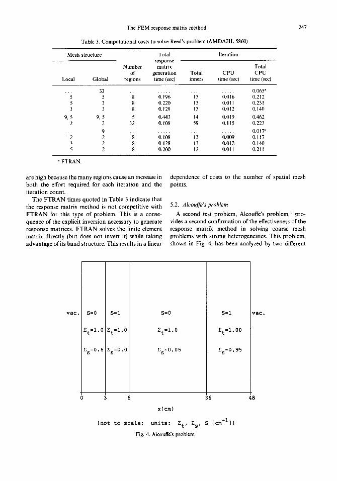
5.2. Alcouffe's problem A second test problem, Alcouffe's problem,1 pro-
vides a second confirmation of the effectiveness of the response matrix method in solving coarse mesh problems with strong heterogeneities. This problem, shown in Fig. 4, has been analyzed by two different
vac. S=0 S=I
Zt=l.0 Et=l.0
Zs=0.5 Zs=0.0
S=0
Zt=l.0
E =0.05 S
S=I
Et=l.00
~s=0.95
vac.
6 36
x(cm)
(not to scale; units: Et, Zs, S [cm-l])
Fig. 4. Alcou~'sproblem.
48
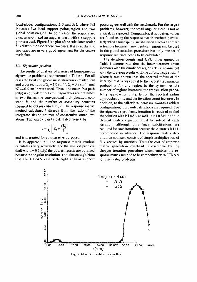
248 J.A. RATHKOPF and W. R. MARTIN
local/global configurations, 5:5 and 5: 2, where 5:2 indicates five local support points/region and two global points/region. In both cases, the regions are 3 cm in width and an angular mesh with six support points is used. Figure 5 is a plot of the calculated scalar flux distributions for these two cases. It is clear that the two cases are in very good agreement for the coarse mesh flux.
5.3. Eigenvalue problem The results of analysis of a series of homogeneous
eigenvalue problems are presented in Table 4. For all cases the local and global mesh structures are identical and cross sections ofE t = 1.0 cm- 1, E~ = 0.5 cm- 1 and vZj.=0.5 cm-~ were used. Thus, one mean free path (mfp) is equivalent to 1 cm. Eigenvalues are presented in two forms: the conventional multiplication con- stant, k, and the number of secondary neutrons required to obtain criticality, c. The response matrix method calculates k directly from the ratio of the integrated fission sources of consecutive outer iter- ations. The value c can be calculated from k by
and is presented for comparative purposes. It is apparent that the response matrix method
calculates k very accurately. For the smallest problem (half-width = 0.5 mfp) the poorest results are obtained because the angular resolution is not fine enough.Note that the FTRAN case with eight angular support
points agrees well with the benchmark. For the largest problems, however, the small angular mesh is not as critical, as expected. Comparable, if not better, values are found using the response matrix method, particu- larly when a finer spatial mesh is used. Such a fine mesh is feasible because many identical regions can be used in the global solution procedure but only one set of response matrices needs to be calculated.
The iteration counts and CPU times quoted in Table 4 demonstrate that the inner iteration count increases with the number of regions. This is consistent with the previous results with the diffusion equation, t where it was shown that the spectral radius of the iteration matrix was equal to the largest transmission probability for any region in the system. As the number of regions increases, the transmission proba- bility approaches unity, hence the spectral radius approaches unity and the iteration count increases. In addition, as the half-width increases towards a critical configuration, more outer iterations are required. For the eigenvalue problems, iteration is required to find the solution with FTRAN as well. In FTRAN the finite element matrix equation must be solved at each iteration, although only back substitutions are required for each iteration because the A matrix is LU- decomposed in advance. The response matrix iter- ation, in contrast, consists of simple multiplication of flux vectors by matrices. Thus the cost of response matrix generation overhead is overcome by the cheaper iteration procedure which enables the re- sponse matrix method to be competitive with FTRAN for eigenvalue problems.
o o o,
1 region : .5 cm . o 5 " 5
°: °.. + 5 " 2
0 x o ~ .
ffl
~:-
. . . . . . . . . . . . . . . . . . . . . . . . ,
.oo 8.oo ,2.oo ,8.oo 2, .oo 3o.oo 38.oo ,2.oo ,8.oo x(cm)
Fig. 5. Alcouffe's problem: scalar flux.

The FEM response matrix method 249
0
©
b.,
n ~
I
Z .<
0 ¢:a
0
0
8
e~ 0
' 0 0
e~
~ d 0~
m
e ~ z ~
i O
I
~:=&&
O ~ O O

250 J.A. RATHKOPF and W. R. MARTIN
6. SUMMARY AND CONCLUSIONS
In this paper, a response matrix method has been developed for solution of the neutron transport equation. The method uses the phase space finite element method as applied to the first-order form of the transport equation as its theoretical foundation. The response matrices have been formulated in such a way as to remove their dependence on the multiplica- tion constant in eigenvalue problems. The response matrices are calculated only once, at the beginning of the problem, for each unique spatial region.
An additional feature of the present method is the two level structure of the spatial and angular discreti- zation. The lower level (local level) is a fine mesh, chosen to resolve the internal heterogeneities satisfac- torily. The upper level (global level) is a coarser mesh which results in a reduction in computat ional expense, while retaining information obtained with the local calculation.
The method as applied to one-dimensional geome- tries has been tested through several benchmark problems. For a given spatial mesh size, the response matrix method gave results nearly identical to those of the conventional finite element method. Superior coarse mesh results were obtained, however, using the local-to-global projection technique. The response matrix method was found to be more efficient than the conventional finite element method in one-dimen- sional slab geometry for only the criticality problem.
Although no two-dimensional results were pre- sented in this paper, preliminary results 44 indicate that the present method is nearly an order of magnitude more efficient than the conventional finite element method in two dimensions. Additional work is required, however, to substantiate these results for different two-dimensional configurations, including the ray effect problem. This will be the subject of a future paper.
REFERENCES
1. Alcouffe R. E., Larsen E. W., Miller W. F. and Wienke B. R. (1979) Computational efficiency of numerical methods for the multi-group, discrete ordinates neutron transport equation: The slab geometry case, Nuel. Sci. Enong 71, 111.
2. Briggs L. L. and Lewis E. E. (1977) A comparison of constrained finite elements and response matrices as one- dimensional transport approximations. Nucl. Sci. Engng 63, 225.
3. Briggs L. L. and Lewis E. E. (1980) A two-dimensional constrained finite element method for nonuniform lattice problems, Nucl. Sci. Engng 75, 76.
4. Kaper H. G., Lindeman A. J. and Leaf G. K. (1974) Benchmark values for the slab and sphere criticality problem in one-group neutron transport theory. Nucl. Sci. Engng 54, 94.
5. Lorence L. J. (1984) An explicitly-interfaced finite element solution of the neutron transport equation, Ph.D. Dissertation, The University of Michigan, Department of Nuclear Engineering, Ann Arbor, MI, U.S.A.
6. Lorence L. J., Martin W. R. and Luskin M. (1985) Analysis of a block gauss-seidel iterative method for a finite element discretization of the neutron transport equation. Trans. Th. Stat. Phy. 14, 35.
7. Martin W. R. and Duderstadt J. J. (1977) Finite element solution of the neutron transport equation with appli- cations to strong heterogeneities. Nucl. Sci. Engn 9 62, 371.
8. Martin W. R., Yehnert C. E., Lorence L. and Duderstadt J. J. (1981) Phase-space finite element methods applied to the first-order form of the transport equation, Ann. Nucl. Energy 8, 633.
9. Miller W. F., Lewis E. E. and Rossow E. C. (1973) The application of phase-space finite elements to the one- dimensional neutron transport equation. Nucl. Sci. Engng 51, 148.
10. Miller W. F., Lewis E. E. and Rossow E. C. (1973) The application of phase space finite elements to the two- dimensional neutron transport equation in X Ygeometry, Nucl. Sci. Engn 9 52, 12.
11. Nakata H. (1981) The finite element response matrix method for coarse mesh reactor analysis, Ph.D. Disser- tation, The University of Michigan, Department of Nuclear Engineering, Ann Arbor, MI, U.S.A.
12. Nakata H. and Martin W. R. (1983) The finite element response matrix method. Nucl. Sci. Eng. 85, 289.
13. Plechaty E. F. and Kimlinger J. R. (1976) TARTNP: A coupled neutron-photon Monte Carlo transport code. UCRL-50400, Lawrence Livermore Laboratory.
14. Rathkopf J. A. (1984) Finite element response matrix method for the solution of the transport equation, Ph.D. Dissertation, The University of Michigan, Department of Nuclear Engineering, Ann Arbor, MI, U.S.A.
15. Reed W. H. (1971) New difference schemes for the neutron transport equation, Nucl. Sei. Engng 46, 309.
16. Yehnert C. E. (1978) Finite element solution of the two- dimensional neutron transport equation, Ph.D. Disser- tation, The University of Michigan, Department of Nuclear Engineering, Ann Arbor, MI, U.S.A.


![MICROSTRUCTURE-BASED FINITE ELEMENT · PDF file3 MICROSTRUCTURE-BASED FINITE ELEMENT MODELING OF PARTICLE REINFORCED METAL MATRIX COMPOSITES extensively [20, 21]](https://img.dokumen.tips/doc/110x75/5a78bc737f8b9a83238bb5cc/microstructure-based-finite-element-microstructure-based-finite-element-modeling.jpg)