Embed Size (px)
Citation preview
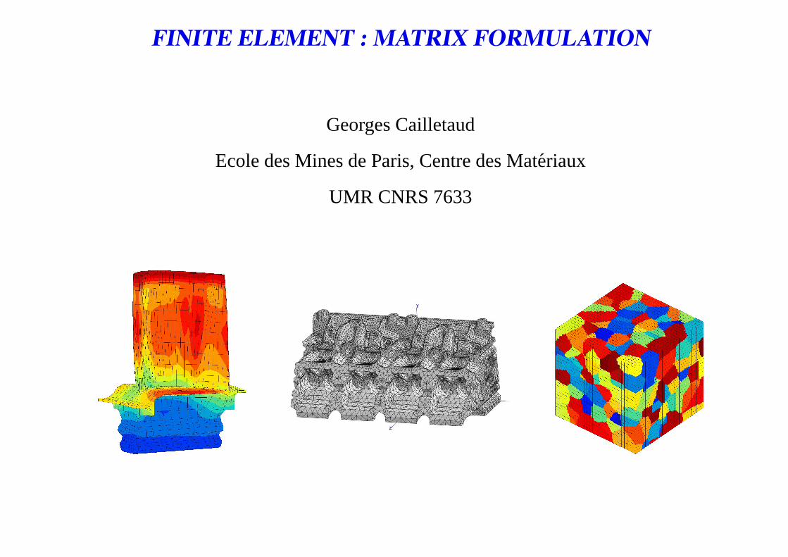
FINITE ELEMENT : MATRIX FORMULATION
Georges Cailletaud
Ecole des Mines de Paris, Centre des Materiaux
UMR CNRS 7633
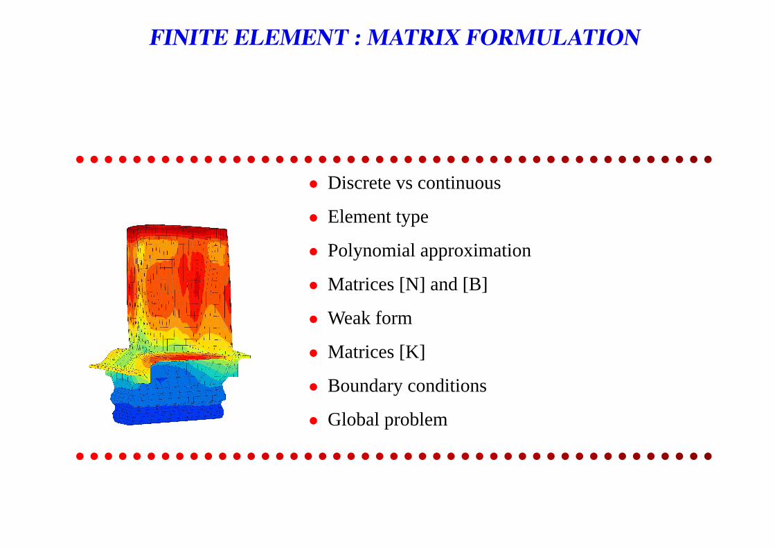
FINITE ELEMENT : MATRIX FORMULATION
• • • • • • • • • • • • • • • • • • • • • • • • • • • • • • • • • • • • • • • • • • • • •• Discrete vs continuous
• Element type
• Polynomial approximation
• Matrices [N] and [B]
• Weak form
• Matrices [K]
• Boundary conditions
• Global problem
• • • • • • • • • • • • • • • • • • • • • • • • • • • • • • • • • • • • • • • • • • • • •
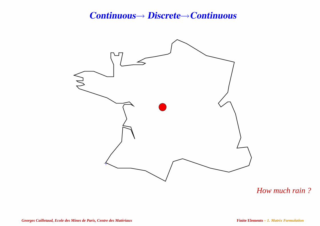
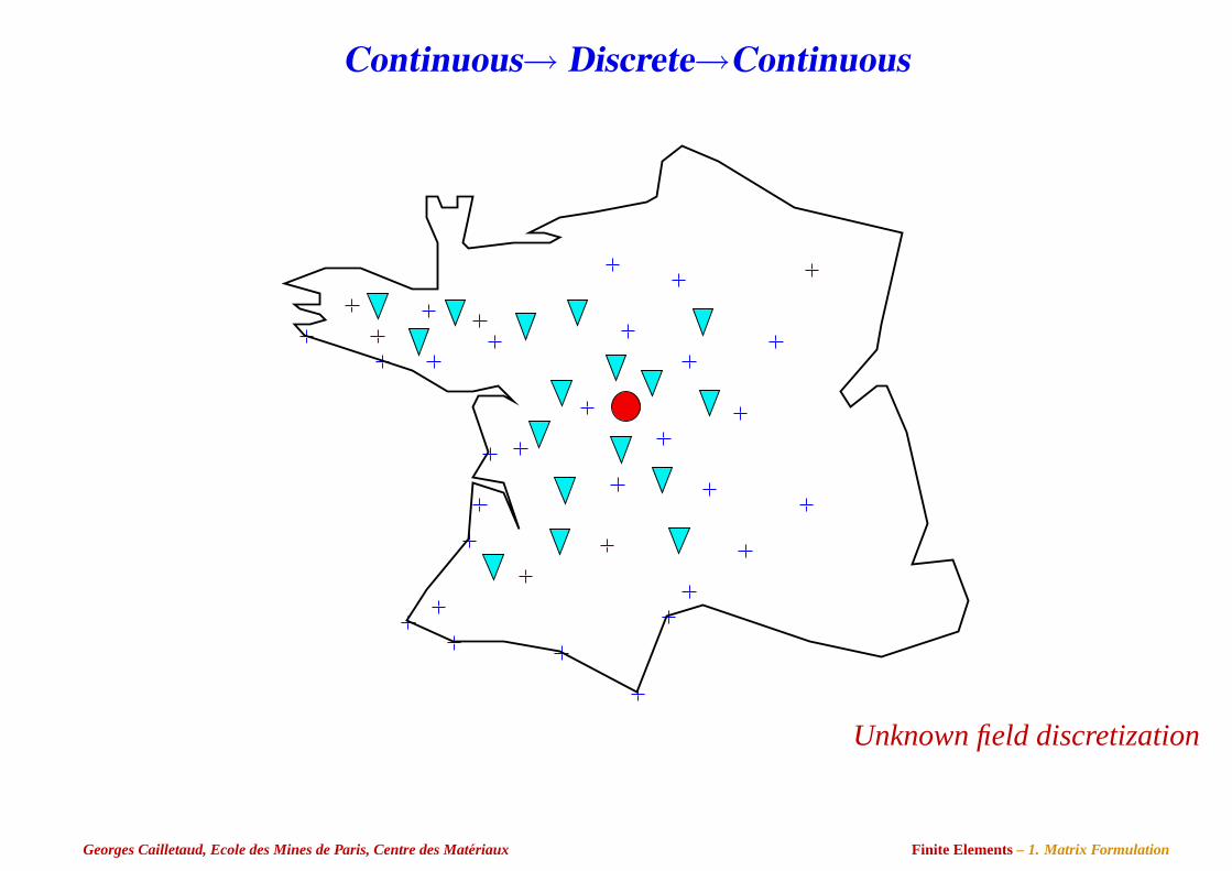
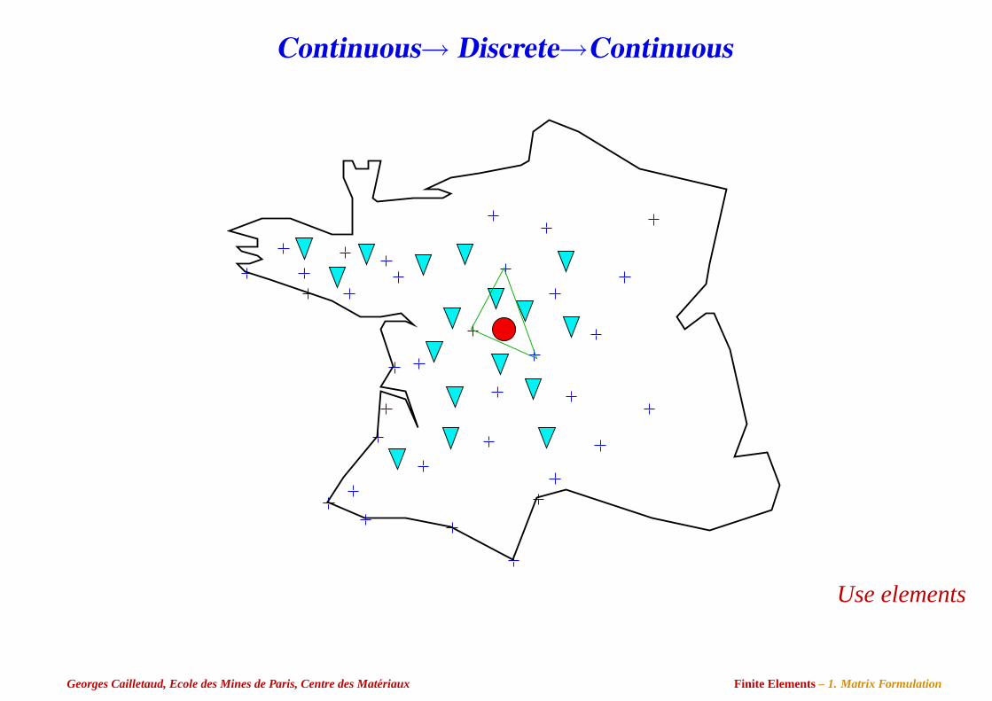
Continuous→ Discrete→Continuous
How much rain ?
Georges Cailletaud, Ecole des Mines de Paris, Centre des Materiaux Finite Elements– 1. Matrix Formulation
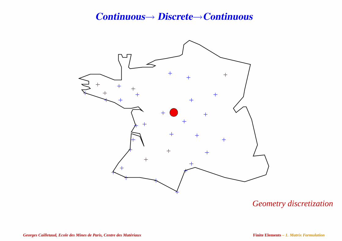
Continuous→ Discrete→Continuous
Geometry discretization
Georges Cailletaud, Ecole des Mines de Paris, Centre des Materiaux Finite Elements– 1. Matrix Formulation
Continuous→ Discrete→Continuous
Unknown field discretization
Georges Cailletaud, Ecole des Mines de Paris, Centre des Materiaux Finite Elements– 1. Matrix Formulation
Continuous→ Discrete→Continuous
Use elements
Georges Cailletaud, Ecole des Mines de Paris, Centre des Materiaux Finite Elements– 1. Matrix Formulation
Finite Element Discretization
Replace continuum formulation by adiscrete representationfor unknownsandgeometry
• Unknown field:
ue(M) =∑
i
Nei (M)qe
i
• Geometry:
x(M) =∑
i
N∗ei (M)x(Pi)
InterpolationfunctionsNei andshapefunctionsN∗e
i such as:
∀M,∑
i
Nei (M) = 1 andNe
i (Pj) = δij
Isoparametricelements iffNei ≡ N∗e
i
Georges Cailletaud, Ecole des Mines de Paris, Centre des Materiaux Finite Elements– 1. Matrix Formulation
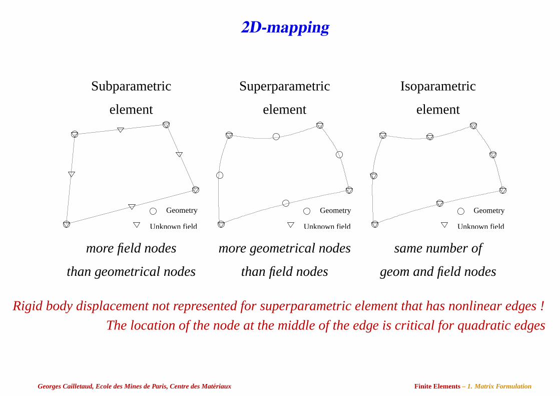
2D-mapping
Subparametric Superparametric Isoparametric
element element element
Geometry
Unknown field
Geometry
Unknown field
Geometry
Unknown field
more field nodes more geometrical nodes same number of
than geometrical nodes than field nodes geom and field nodes
Rigid body displacement not represented for superparametric element that has nonlinear edges !
The location of the node at the middle of the edge is critical for quadratic edges
Georges Cailletaud, Ecole des Mines de Paris, Centre des Materiaux Finite Elements– 1. Matrix Formulation
Shape function matrix, [N] – Deformation matrix, [B]
• Fieldu, T , C
• Gradientε∼, grad(T ),. . .
• Constitutive equationsσ∼ = Λ∼∼: ε∼, q = −kgrad(T )
• Conservationdiv(σ∼) + f = 0, . . .
First step: express the continuous field and its gradient wrt the discretized vector
Georges Cailletaud, Ecole des Mines de Paris, Centre des Materiaux Finite Elements– 1. Matrix Formulation
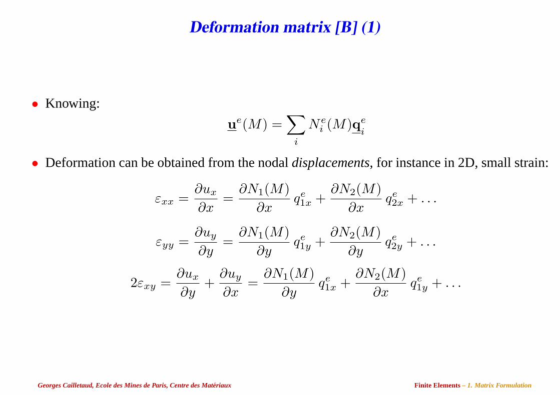
Deformation matrix [B] (1)
• Knowing:
ue(M) =∑
i
Nei (M)qe
i
• Deformation can be obtained from the nodaldisplacements, for instance in 2D, small strain:
εxx =∂ux
∂x=
∂N1(M)∂x
qe1x +
∂N2(M)∂x
qe2x + . . .
εyy =∂uy
∂y=
∂N1(M)∂y
qe1y +
∂N2(M)∂y
qe2y + . . .
2εxy =∂ux
∂y+
∂uy
∂x=
∂N1(M)∂y
qe1x +
∂N2(M)∂x
qe1y + . . .
Georges Cailletaud, Ecole des Mines de Paris, Centre des Materiaux Finite Elements– 1. Matrix Formulation
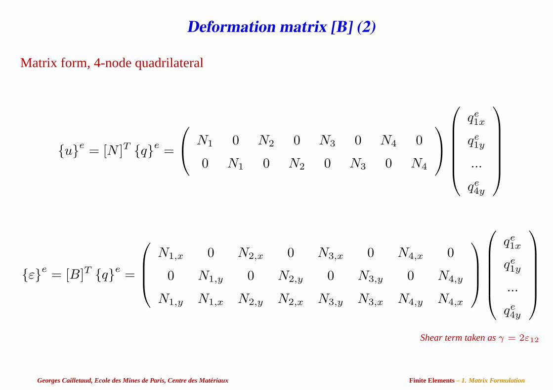
Deformation matrix [B] (2)
Matrix form, 4-node quadrilateral
ue = [N ]T qe =
N1 0 N2 0 N3 0 N4 0
0 N1 0 N2 0 N3 0 N4
qe1x
qe1y
...
qe4y
εe = [B]T qe =
N1,x 0 N2,x 0 N3,x 0 N4,x 0
0 N1,y 0 N2,y 0 N3,y 0 N4,y
N1,y N1,x N2,y N2,x N3,y N3,x N4,y N4,x
qe1x
qe1y
...
qe4y
Shear term taken asγ = 2ε12
Georges Cailletaud, Ecole des Mines de Paris, Centre des Materiaux Finite Elements– 1. Matrix Formulation
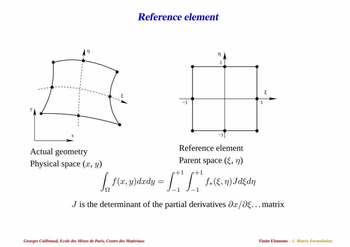
Reference element
x
y
ξ
η
Actual geometry
Physical space (x, y)
η
ξ
1
−1
−1 1
Reference element
Parent space (ξ, η)∫Ω
f(x, y)dxdy =∫ +1
−1
∫ +1
−1
f∗(ξ, η)Jdξdη
J is the determinant of the partial derivatives∂x/∂ξ. . . matrix
Georges Cailletaud, Ecole des Mines de Paris, Centre des Materiaux Finite Elements– 1. Matrix Formulation
Remarks on geometrical mapping
• The values on an edge depends only on the nodal values on the same edge (linear
interpolation equal to zero on each side for 2-node lines, parabolic interpolation equal to
zero for 3 points for 3-node lines)
• Continuity...
• The mid node is used to allow non linear geometries
• Limits in the admissible mapping for avoiding singularities
Georges Cailletaud, Ecole des Mines de Paris, Centre des Materiaux Finite Elements– 1. Matrix Formulation
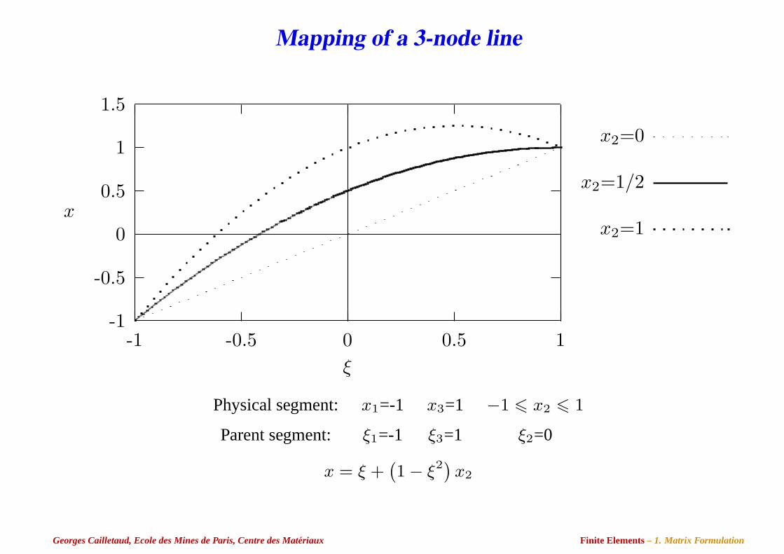
Mapping of a 3-node line
-1
-0.5
0
0.5
1
1.5
-1 -0.5 0 0.5 1
x
ξ
x2=0
x2=1/2
x2=1
Physical segment: x1=-1 x3=1 −1 6 x2 6 1
Parent segment: ξ1=-1 ξ3=1 ξ2=0
x = ξ +(1− ξ2) x2
Georges Cailletaud, Ecole des Mines de Paris, Centre des Materiaux Finite Elements– 1. Matrix Formulation
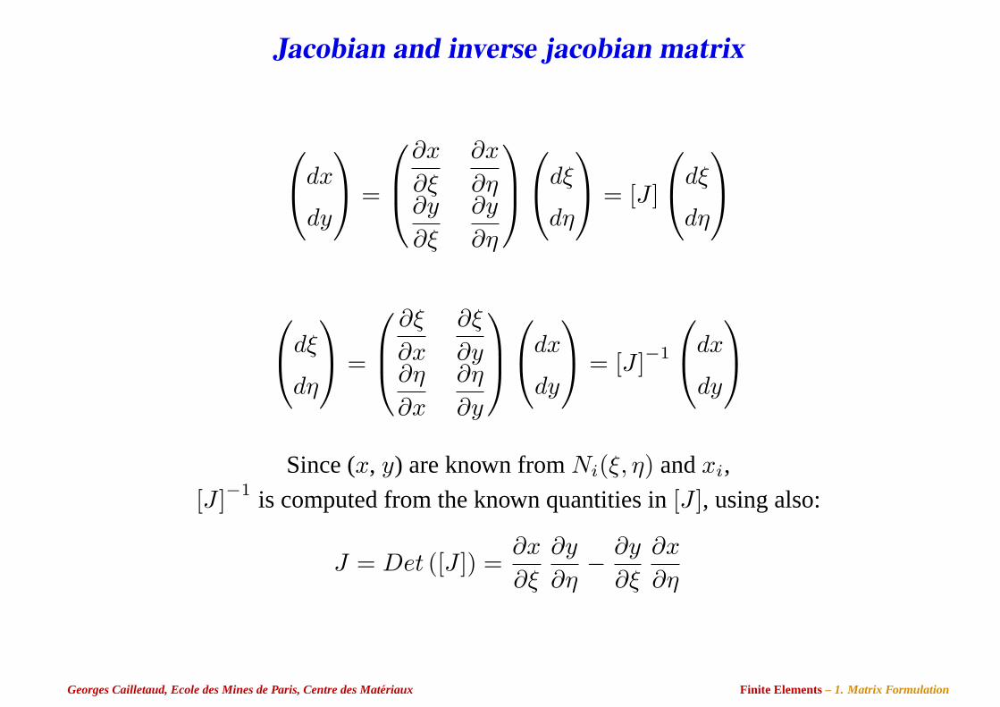
Jacobian and inverse jacobian matrix
dx
dy
=
∂x
∂ξ
∂x
∂η∂y
∂ξ
∂y
∂η
dξ
dη
= [J ]
dξ
dη
dξ
dη
=
∂ξ
∂x
∂ξ
∂y∂η
∂x
∂η
∂y
dx
dy
= [J ]−1
dx
dy
Since (x, y) are known fromNi(ξ, η) andxi,
[J ]−1 is computed from the known quantities in[J ], using also:
J = Det ([J ]) =∂x
∂ξ
∂y
∂η− ∂y
∂ξ
∂x
∂η
Georges Cailletaud, Ecole des Mines de Paris, Centre des Materiaux Finite Elements– 1. Matrix Formulation
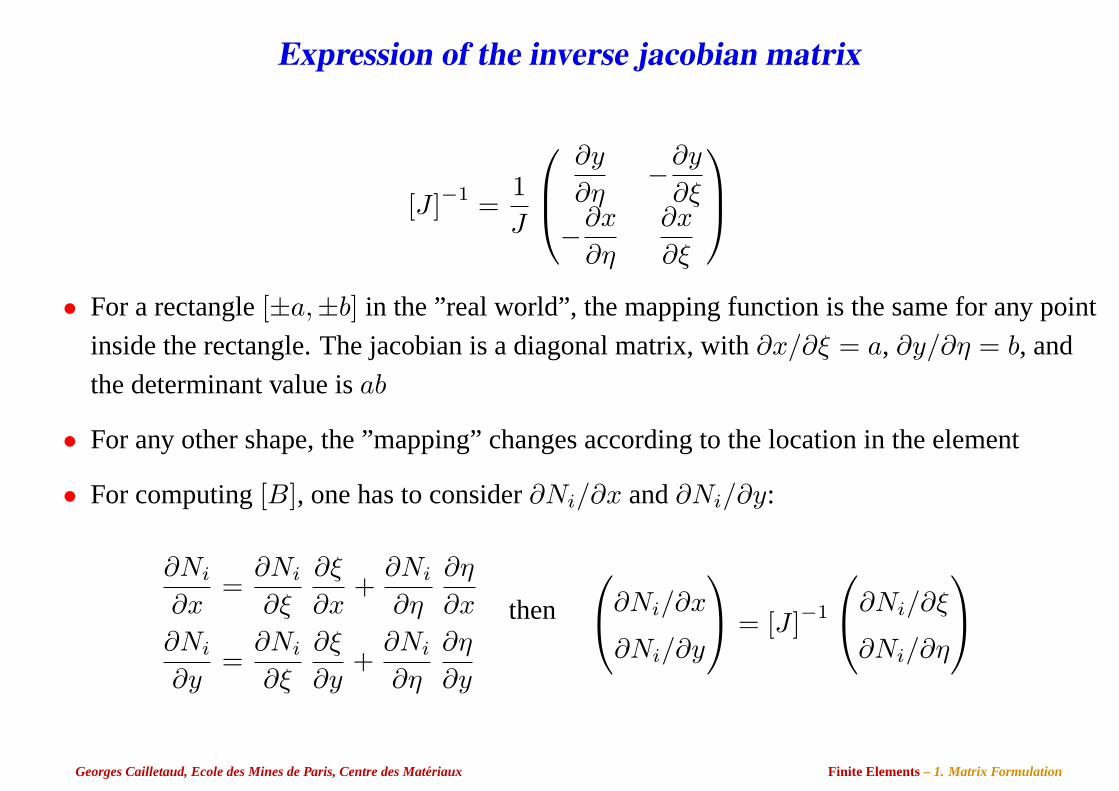
Expression of the inverse jacobian matrix
[J ]−1 =1J
∂y
∂η−∂y
∂ξ
−∂x
∂η
∂x
∂ξ
• For a rectangle[±a,±b] in the ”real world”, the mapping function is the same for any point
inside the rectangle. The jacobian is a diagonal matrix, with∂x/∂ξ = a, ∂y/∂η = b, and
the determinant value isab
• For any other shape, the ”mapping” changes according to the location in the element
• For computing[B], one has to consider∂Ni/∂x and∂Ni/∂y:
∂Ni
∂x=
∂Ni
∂ξ
∂ξ
∂x+
∂Ni
∂η
∂η
∂x
∂Ni
∂y=
∂Ni
∂ξ
∂ξ
∂y+
∂Ni
∂η
∂η
∂y
then
∂Ni/∂x
∂Ni/∂y
= [J ]−1
∂Ni/∂ξ
∂Ni/∂η
Georges Cailletaud, Ecole des Mines de Paris, Centre des Materiaux Finite Elements– 1. Matrix Formulation
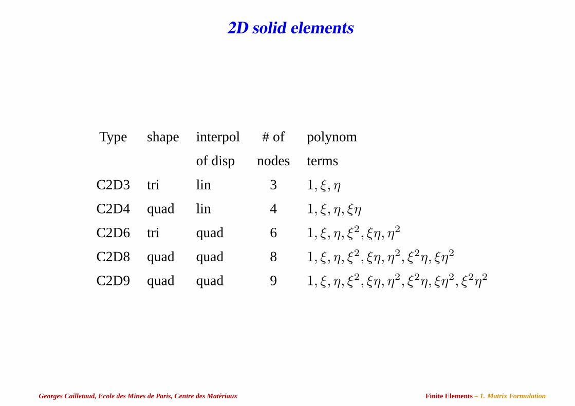
2D solid elements
Type shape interpol # of polynom
of disp nodes terms
C2D3 tri lin 3 1, ξ, η
C2D4 quad lin 4 1, ξ, η, ξη
C2D6 tri quad 6 1, ξ, η, ξ2, ξη, η2
C2D8 quad quad 8 1, ξ, η, ξ2, ξη, η2, ξ2η, ξη2
C2D9 quad quad 9 1, ξ, η, ξ2, ξη, η2, ξ2η, ξη2, ξ2η2
Georges Cailletaud, Ecole des Mines de Paris, Centre des Materiaux Finite Elements– 1. Matrix Formulation
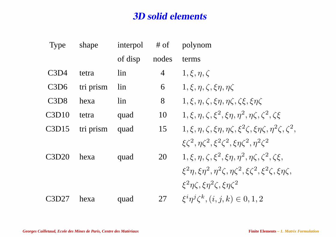
3D solid elements
Type shape interpol # of polynom
of disp nodes terms
C3D4 tetra lin 4 1, ξ, η, ζ
C3D6 tri prism lin 6 1, ξ, η, ζ, ξη, ηζ
C3D8 hexa lin 8 1, ξ, η, ζ, ξη, ηζ, ζξ, ξηζ
C3D10 tetra quad 10 1, ξ, η, ζ, ξ2, ξη, η2, ηζ, ζ2, ζξ
C3D15 tri prism quad 15 1, ξ, η, ζ, ξη, ηζ, ξ2ζ, ξηζ, η2ζ, ζ2,
ξζ2, ηζ2, ξ2ζ2, ξηζ2, η2ζ2
C3D20 hexa quad 20 1, ξ, η, ζ, ξ2, ξη, η2, ηζ, ζ2, ζξ,
ξ2η, ξη2, η2ζ, ηζ2, ξζ2, ξ2ζ, ξηζ,
ξ2ηζ, ξη2ζ, ξηζ2
C3D27 hexa quad 27 ξiηjζk, (i, j, k) ∈ 0, 1, 2
Georges Cailletaud, Ecole des Mines de Paris, Centre des Materiaux Finite Elements– 1. Matrix Formulation
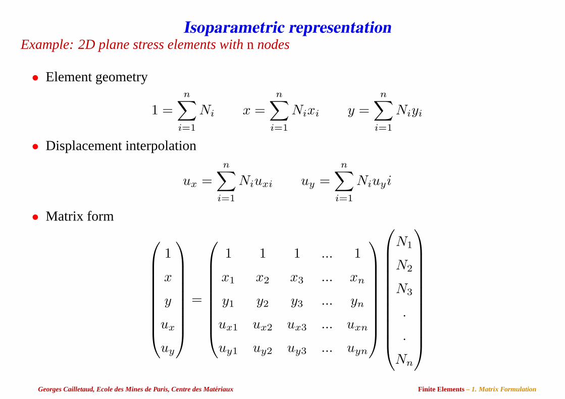
Isoparametric representationExample: 2D plane stress elements withn nodes
• Element geometry
1 =n∑
i=1
Ni x =n∑
i=1
Nixi y =n∑
i=1
Niyi
• Displacement interpolation
ux =n∑
i=1
Niuxi uy =n∑
i=1
Niuyi
• Matrix form
1
x
y
ux
uy
=
1 1 1 ... 1
x1 x2 x3 ... xn
y1 y2 y3 ... yn
ux1 ux2 ux3 ... uxn
uy1 uy2 uy3 ... uyn
N1
N2
N3
.
.
Nn
Georges Cailletaud, Ecole des Mines de Paris, Centre des Materiaux Finite Elements– 1. Matrix Formulation
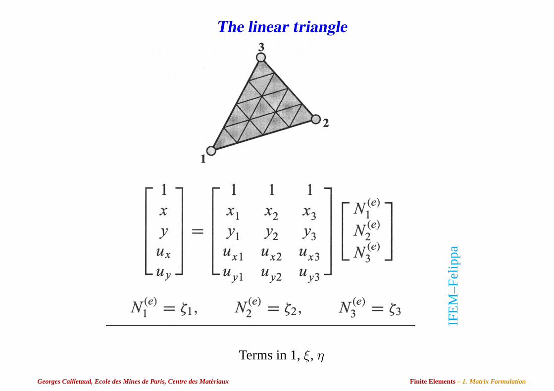
The linear triangle
IFE
M–F
elip
pa
Terms in 1,ξ, η
Georges Cailletaud, Ecole des Mines de Paris, Centre des Materiaux Finite Elements– 1. Matrix Formulation
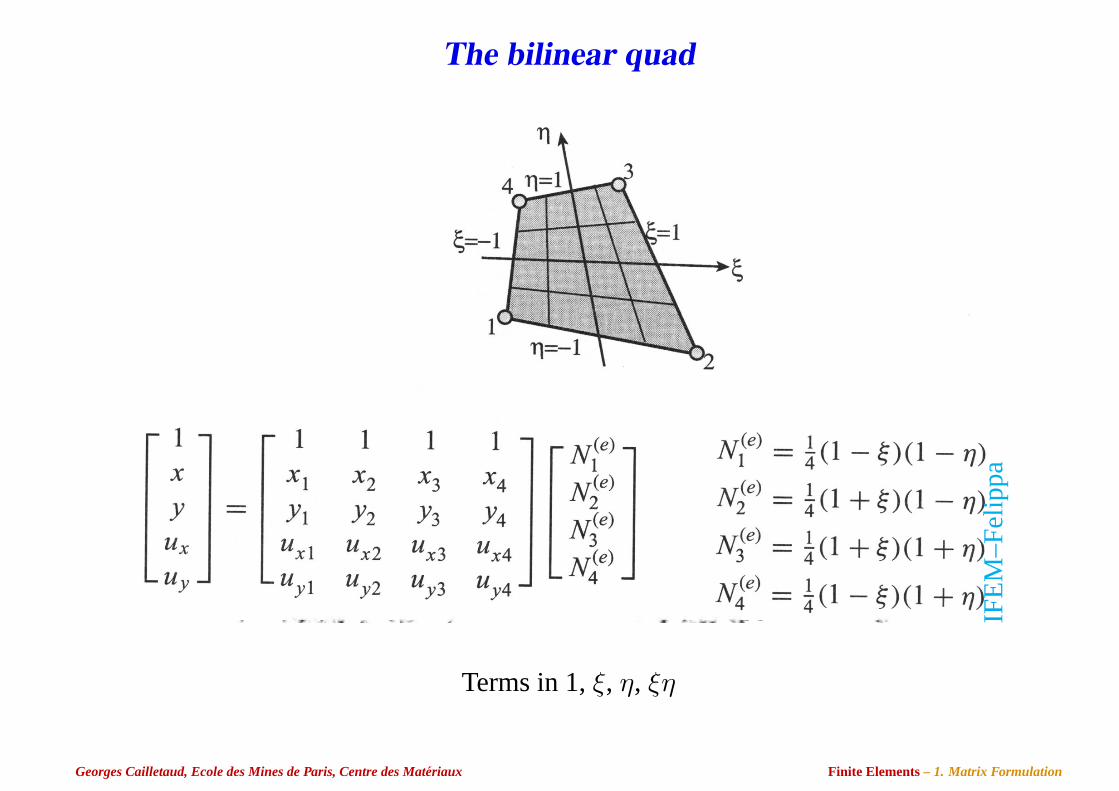
The bilinear quad
IFE
M–F
elip
pa
Terms in 1,ξ, η, ξη
Georges Cailletaud, Ecole des Mines de Paris, Centre des Materiaux Finite Elements– 1. Matrix Formulation
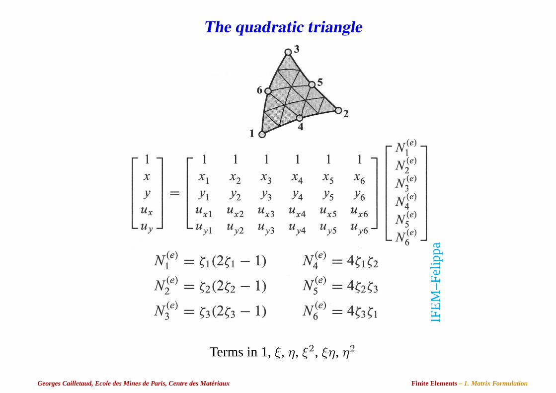
The quadratic triangle
IFE
M–F
elip
pa
Terms in 1,ξ, η, ξ2, ξη, η2
Georges Cailletaud, Ecole des Mines de Paris, Centre des Materiaux Finite Elements– 1. Matrix Formulation
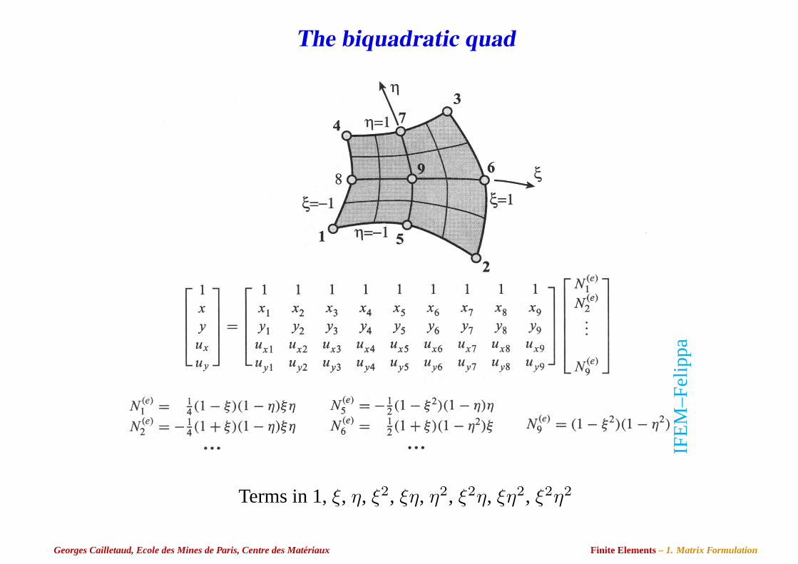
The biquadratic quad
IFE
M–F
elip
pa
Terms in 1,ξ, η, ξ2, ξη, η2, ξ2η, ξη2, ξ2η2
Georges Cailletaud, Ecole des Mines de Paris, Centre des Materiaux Finite Elements– 1. Matrix Formulation
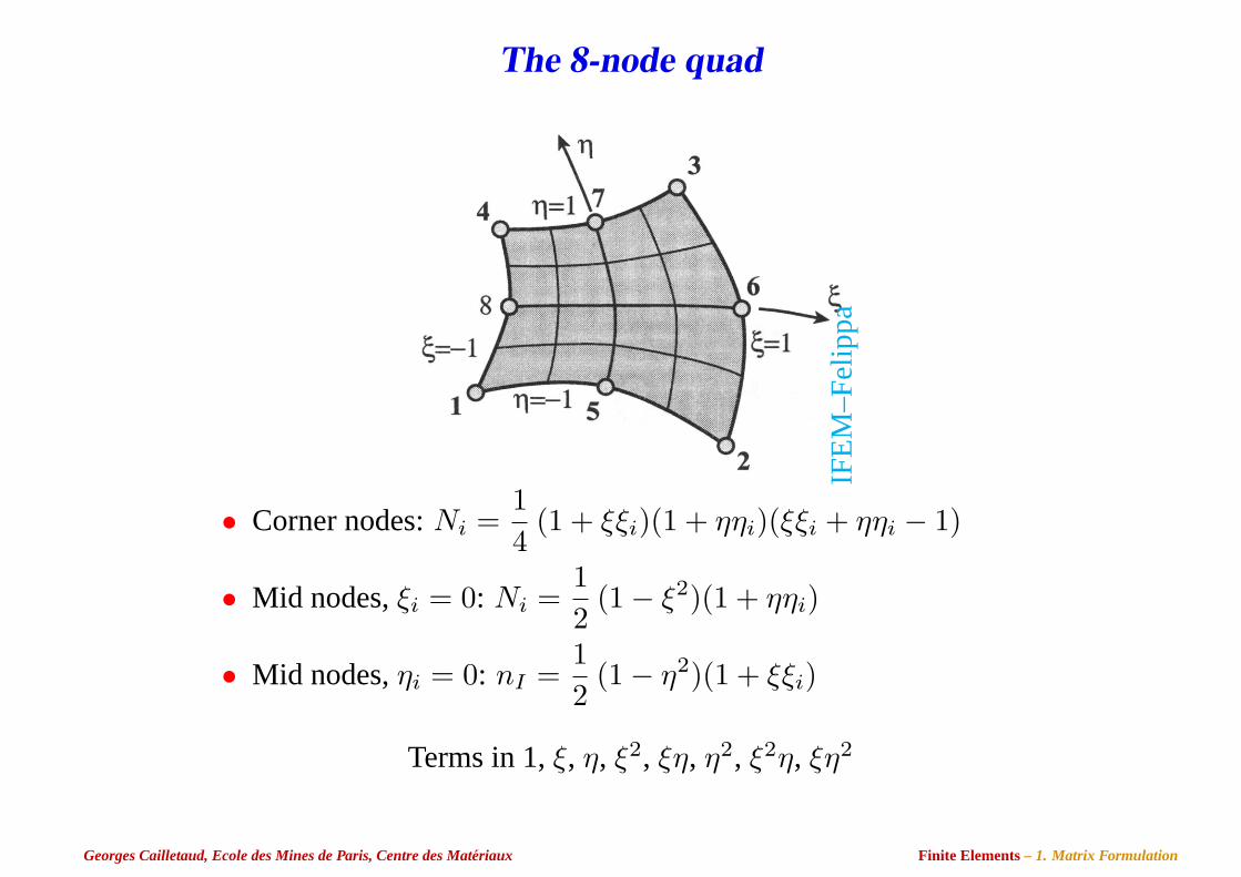
The 8-node quad
IFE
M–F
elip
pa
• Corner nodes:Ni =14
(1 + ξξi)(1 + ηηi)(ξξi + ηηi − 1)
• Mid nodes,ξi = 0: Ni =12
(1− ξ2)(1 + ηηi)
• Mid nodes,ηi = 0: nI =12
(1− η2)(1 + ξξi)
Terms in 1,ξ, η, ξ2, ξη, η2, ξ2η, ξη2
Georges Cailletaud, Ecole des Mines de Paris, Centre des Materiaux Finite Elements– 1. Matrix Formulation
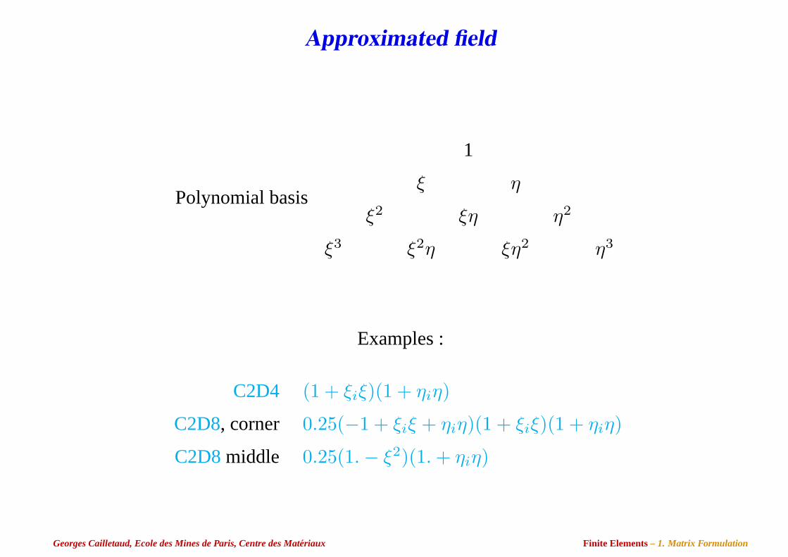
Approximated field
Polynomial basis
1
ξ η
ξ2 ξη η2
ξ3 ξ2η ξη2 η3
Examples :
C2D4 (1 + ξiξ)(1 + ηiη)
C2D8, corner 0.25(−1 + ξiξ + ηiη)(1 + ξiξ)(1 + ηiη)
C2D8middle 0.25(1.− ξ2)(1. + ηiη)
Georges Cailletaud, Ecole des Mines de Paris, Centre des Materiaux Finite Elements– 1. Matrix Formulation
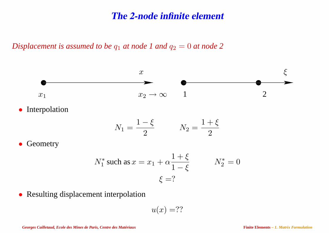
The 2-node infinite element
Displacement is assumed to beq1 at node 1 andq2 = 0 at node 2
x ξ
x1 x2 →∞ 1 2
• Interpolation
N1 =1− ξ
2N2 =
1 + ξ
2• Geometry
N∗1 such asx = x1 + α
1 + ξ
1− ξN∗
2 = 0
ξ =?
• Resulting displacement interpolation
u(x) =??
Georges Cailletaud, Ecole des Mines de Paris, Centre des Materiaux Finite Elements– 1. Matrix Formulation
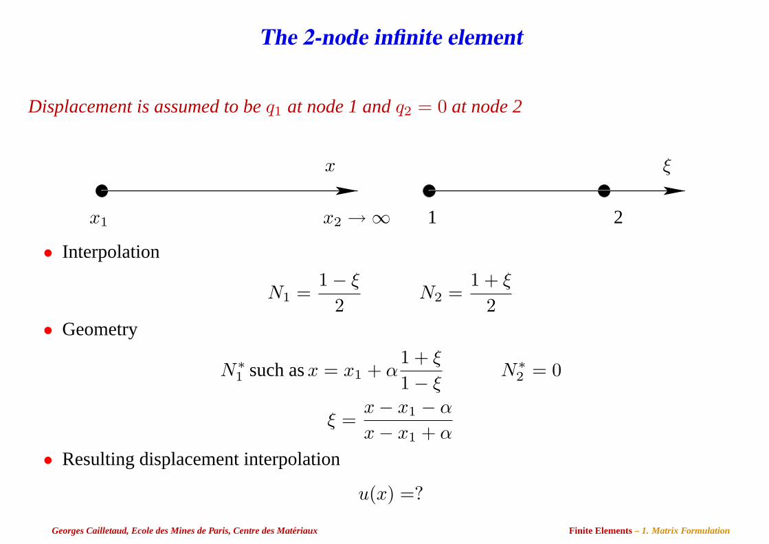
The 2-node infinite element
Displacement is assumed to beq1 at node 1 andq2 = 0 at node 2
x ξ
x1 x2 →∞ 1 2
• Interpolation
N1 =1− ξ
2N2 =
1 + ξ
2• Geometry
N∗1 such asx = x1 + α
1 + ξ
1− ξN∗
2 = 0
ξ =x− x1 − α
x− x1 + α
• Resulting displacement interpolation
u(x) =?
Georges Cailletaud, Ecole des Mines de Paris, Centre des Materiaux Finite Elements– 1. Matrix Formulation
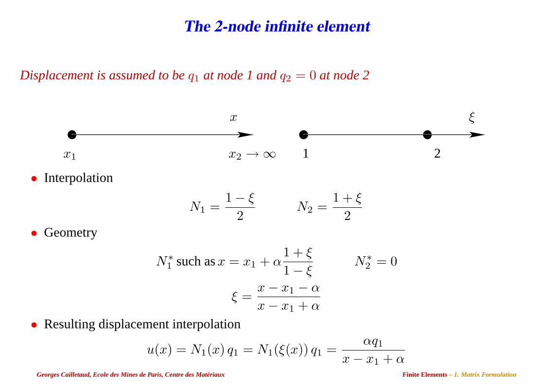
The 2-node infinite element
Displacement is assumed to beq1 at node 1 andq2 = 0 at node 2
x ξ
x1 x2 →∞ 1 2
• Interpolation
N1 =1− ξ
2N2 =
1 + ξ
2• Geometry
N∗1 such asx = x1 + α
1 + ξ
1− ξN∗
2 = 0
ξ =x− x1 − α
x− x1 + α
• Resulting displacement interpolation
u(x) = N1(x) q1 = N1(ξ(x)) q1 =αq1
x− x1 + αGeorges Cailletaud, Ecole des Mines de Paris, Centre des Materiaux Finite Elements– 1. Matrix Formulation
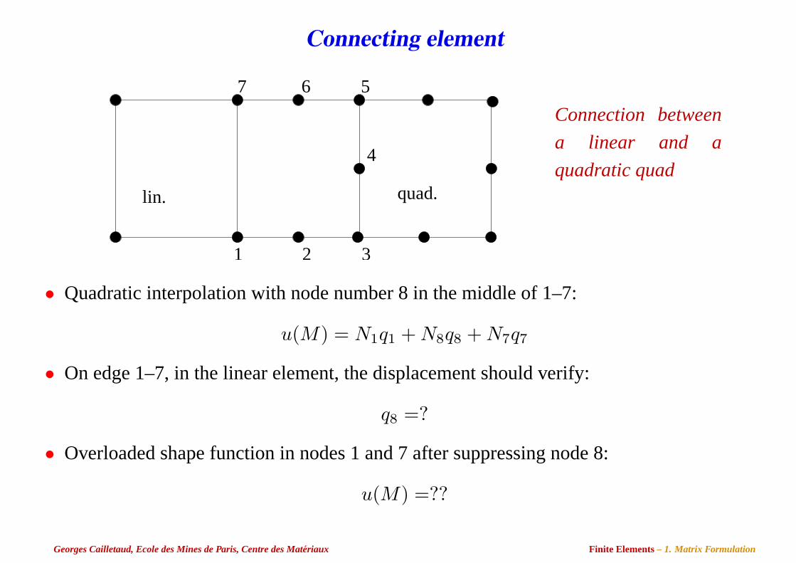
Connecting element
1 2 3
7 6 5
4
lin. quad.
Connection between
a linear and a
quadratic quad
• Quadratic interpolation with node number 8 in the middle of 1–7:
u(M) = N1q1 + N8q8 + N7q7
• On edge 1–7, in the linear element, the displacement should verify:
q8 =?
• Overloaded shape function in nodes 1 and 7 after suppressing node 8:
u(M) =??
Georges Cailletaud, Ecole des Mines de Paris, Centre des Materiaux Finite Elements– 1. Matrix Formulation
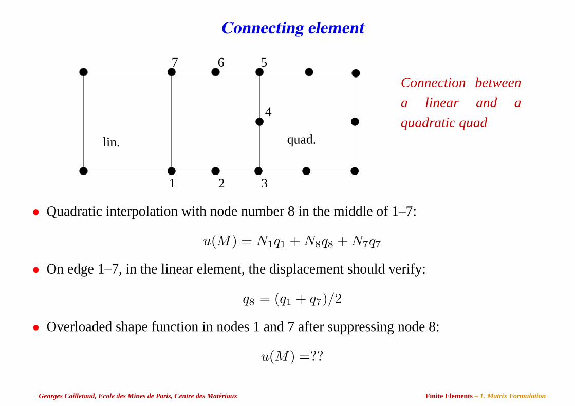
Connecting element
1 2 3
7 6 5
4
lin. quad.
Connection between
a linear and a
quadratic quad
• Quadratic interpolation with node number 8 in the middle of 1–7:
u(M) = N1q1 + N8q8 + N7q7
• On edge 1–7, in the linear element, the displacement should verify:
q8 = (q1 + q7)/2
• Overloaded shape function in nodes 1 and 7 after suppressing node 8:
u(M) =??
Georges Cailletaud, Ecole des Mines de Paris, Centre des Materiaux Finite Elements– 1. Matrix Formulation
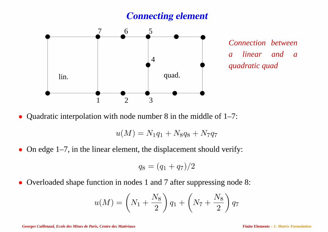
Connecting element
1 2 3
7 6 5
4
lin. quad.
Connection between
a linear and a
quadratic quad
• Quadratic interpolation with node number 8 in the middle of 1–7:
u(M) = N1q1 + N8q8 + N7q7
• On edge 1–7, in the linear element, the displacement should verify:
q8 = (q1 + q7)/2
• Overloaded shape function in nodes 1 and 7 after suppressing node 8:
u(M) =(
N1 +N8
2
)q1 +
(N7 +
N8
2
)q7
Georges Cailletaud, Ecole des Mines de Paris, Centre des Materiaux Finite Elements– 1. Matrix Formulation
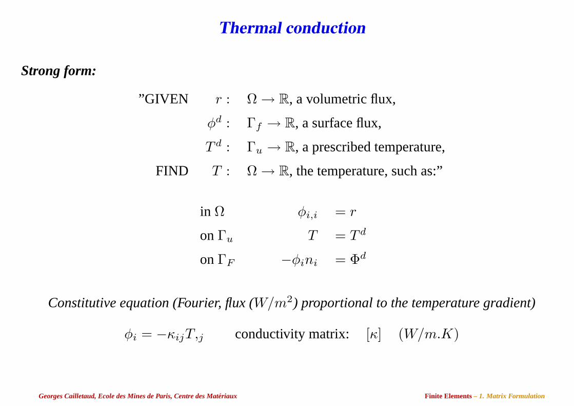
Thermal conduction
Strong form:
”GIVEN r : Ω → R, a volumetric flux,
φd : Γf → R, a surface flux,
T d : Γu → R, a prescribed temperature,
FIND T : Ω → R, the temperature, such as:”
in Ω φi,i = r
onΓu T = T d
onΓF −φini = Φd
Constitutive equation (Fourier, flux (W/m2) proportional to the temperature gradient)
φi = −κijT,j conductivity matrix: [κ] (W/m.K)
Georges Cailletaud, Ecole des Mines de Paris, Centre des Materiaux Finite Elements– 1. Matrix Formulation
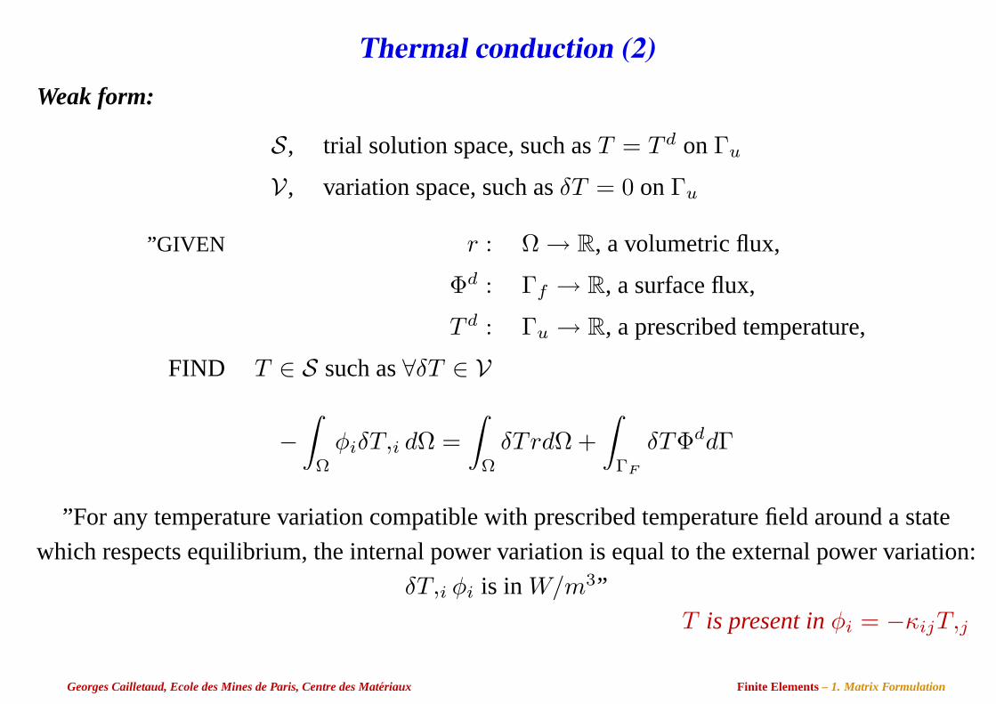
Thermal conduction (2)Weak form:
S, trial solution space, such asT = T d onΓu
V, variation space, such asδT = 0 onΓu
”GIVEN r : Ω → R, a volumetric flux,
Φd : Γf → R, a surface flux,
T d : Γu → R, a prescribed temperature,
FIND T ∈ S such as∀δT ∈ V
−∫
Ω
φiδT,i dΩ =∫
Ω
δTrdΩ +∫
ΓF
δTΦddΓ
”For any temperature variation compatible with prescribed temperature field around a state
which respects equilibrium, the internal power variation is equal to the external power variation:
δT,i φi is in W/m3”
T is present inφi = −κijT,j
Georges Cailletaud, Ecole des Mines de Paris, Centre des Materiaux Finite Elements– 1. Matrix Formulation
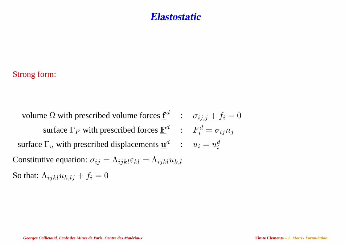
Elastostatic
Strong form:
volumeΩ with prescribed volume forcesfd : σij,j + fi = 0
surfaceΓF with prescribed forcesFd : F di = σijnj
surfaceΓu with prescribed displacementsud : ui = udi
Constitutive equation:σij = Λijklεkl = Λijkluk,l
So that:Λijkluk,lj + fi = 0
Georges Cailletaud, Ecole des Mines de Paris, Centre des Materiaux Finite Elements– 1. Matrix Formulation
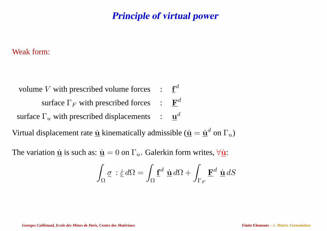
Principle of virtual power
Weak form:
volumeV with prescribed volume forces : fd
surfaceΓF with prescribed forces : Fd
surfaceΓu with prescribed displacements :ud
Virtual displacement rateu kinematically admissible (u = ud onΓu)
The variationu is such as:u = 0 onΓu. Galerkin form writes,∀u:∫Ω
σ∼ : ε∼dΩ =∫
Ω
fd u dΩ +∫
ΓF
Fd u dS
Georges Cailletaud, Ecole des Mines de Paris, Centre des Materiaux Finite Elements– 1. Matrix Formulation
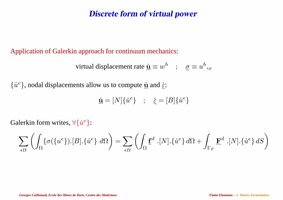
Discrete form of virtual power
Application of Galerkin approach for continuum mechanics:
virtual displacement rateu ≡ wh ; σ∼ ≡ uh,x
ue, nodal displacements allow us to computeu andε∼:
u = [N ]ue ; ε∼ = [B]ue
Galerkin form writes,∀ue:∑elt
(∫Ω
σ(ue).[B].ue dΩ)
=∑elt
(∫Ω
fd .[N ].ue dΩ +∫
ΓF
Fd .[N ].ue dS
)
Georges Cailletaud, Ecole des Mines de Paris, Centre des Materiaux Finite Elements– 1. Matrix Formulation
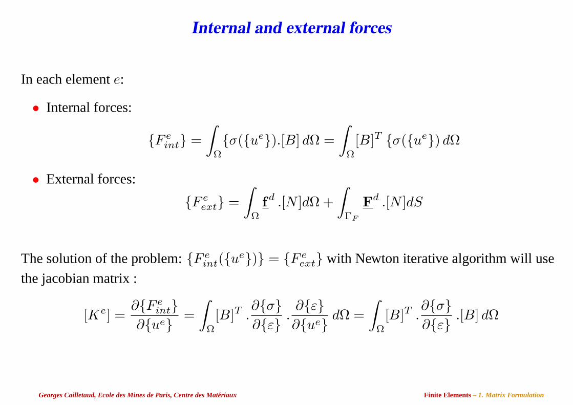
Internal and external forces
In each elemente:
• Internal forces:
F eint =
∫Ω
σ(ue).[B] dΩ =∫
Ω
[B]T σ(ue) dΩ
• External forces:
F eext =
∫Ω
fd .[N ]dΩ +∫
ΓF
Fd .[N ]dS
The solution of the problem:F eint(ue) = F e
ext with Newton iterative algorithm will use
the jacobian matrix :
[Ke] =∂F e
int∂ue
=∫
Ω
[B]T .∂σ∂ε
.∂ε∂ue
dΩ =∫
Ω
[B]T .∂σ∂ε
.[B] dΩ
Georges Cailletaud, Ecole des Mines de Paris, Centre des Materiaux Finite Elements– 1. Matrix Formulation
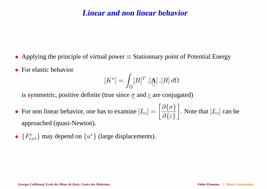
Linear and non linear behavior
• Applying the principle of virtual power≡ Stationnary point of Potential Energy
• For elastic behavior
[Ke] =∫
Ω
[B]T .[Λ∼∼] .[B] dΩ
is symmetric, positive definite (true sinceσ∼ andε∼ are conjugated)
• For non linear behavior, one has to examine[Lc] =[∂σ∂ε
]. Note that[Lc] can be
approached (quasi-Newton).
• F eext may depend onue (large displacements).
Georges Cailletaud, Ecole des Mines de Paris, Centre des Materiaux Finite Elements– 1. Matrix Formulation
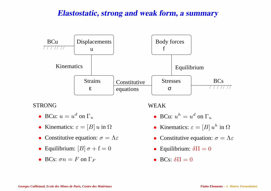
Elastostatic, strong and weak form, a summary
Displacementsu
Body forces f
Strains Stressesε σ
BCu
BCs
Kinematics
Constitutiveequations
Equilibrium
STRONG
• BCu: u = ud onΓu
• Kinematics:ε = [B] u in Ω
• Constitutive equation:σ = Λε
• Equilibrium: [B] σ + f = 0
• BCs:σn = F onΓF
WEAK
• BCu: uh = ud onΓu
• Kinematics:ε = [B] uh in Ω
• Constitutive equation:σ = Λε
• Equilibrium: δΠ = 0
• BCs: δΠ = 0
Georges Cailletaud, Ecole des Mines de Paris, Centre des Materiaux Finite Elements– 1. Matrix Formulation
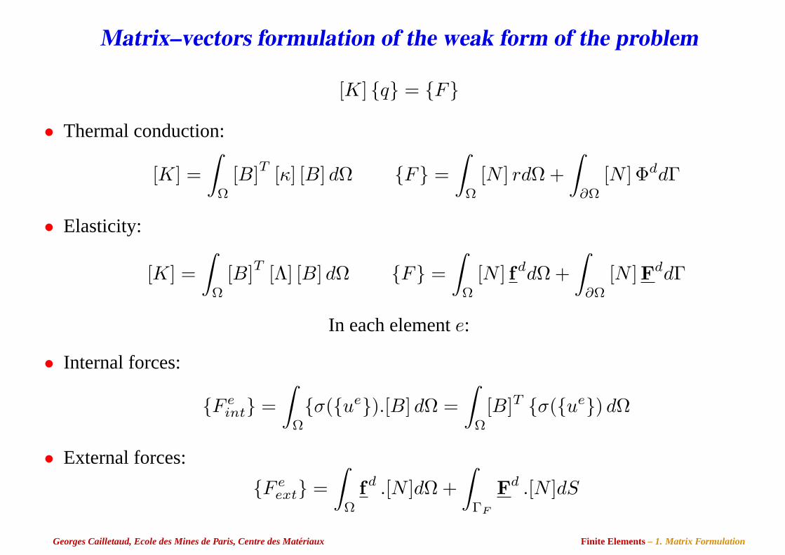
Matrix–vectors formulation of the weak form of the problem
[K] q = F
• Thermal conduction:
[K] =∫
Ω
[B]T [κ] [B] dΩ F =∫
Ω
[N ] rdΩ +∫
∂Ω
[N ] ΦddΓ
• Elasticity:
[K] =∫
Ω
[B]T [Λ] [B] dΩ F =∫
Ω
[N ] fddΩ +∫
∂Ω
[N ]FddΓ
In each elemente:
• Internal forces:
F eint =
∫Ω
σ(ue).[B] dΩ =∫
Ω
[B]T σ(ue) dΩ
• External forces:
F eext =
∫Ω
fd .[N ]dΩ +∫
ΓF
Fd .[N ]dS
Georges Cailletaud, Ecole des Mines de Paris, Centre des Materiaux Finite Elements– 1. Matrix Formulation
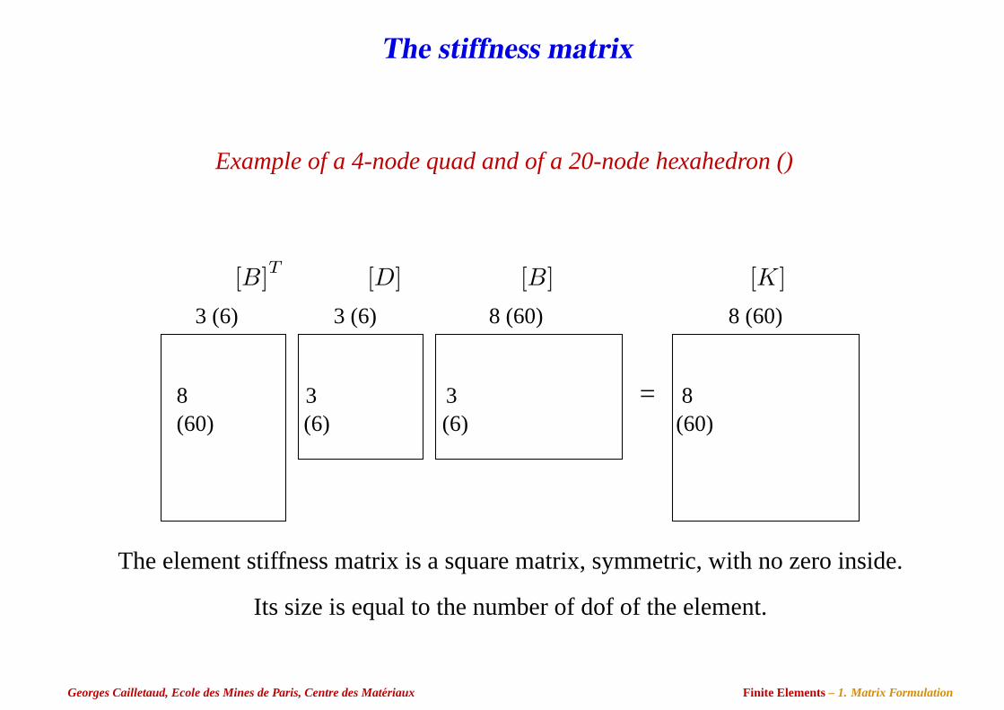
The stiffness matrix
Example of a 4-node quad and of a 20-node hexahedron ()
[B]T [D] [B] [K]
=
3 (6) 3 (6) 8 (60) 8 (60)
8 3 3 8(60) (6) (6) (60)
The element stiffness matrix is a square matrix, symmetric, with no zero inside.
Its size is equal to the number of dof of the element.
Georges Cailletaud, Ecole des Mines de Paris, Centre des Materiaux Finite Elements– 1. Matrix Formulation
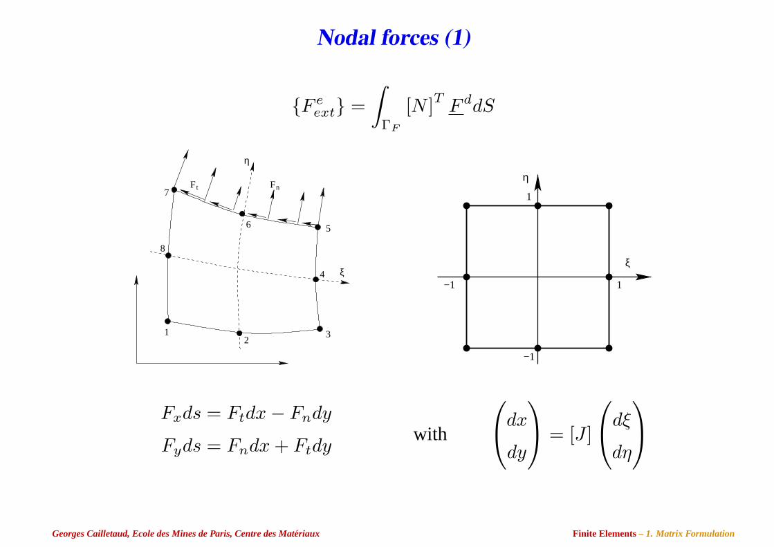
Nodal forces (1)
F eext =
∫ΓF
[N ]T F ddS
Fn
1
5
7F t
8
4
23
6
ξ
η
η
ξ
1
−1
−1 1
Fxds = Ftdx− Fndy
Fyds = Fndx + Ftdywith
dx
dy
= [J ]
dξ
dη
Georges Cailletaud, Ecole des Mines de Paris, Centre des Materiaux Finite Elements– 1. Matrix Formulation
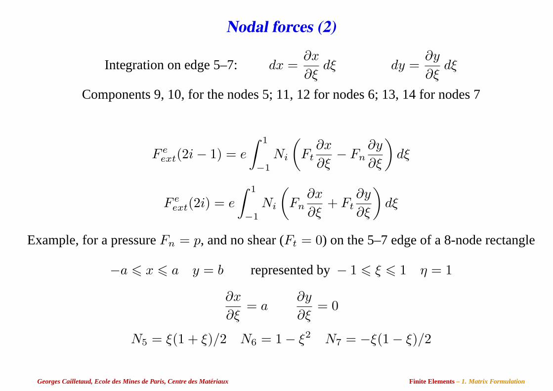
Nodal forces (2)
Integration on edge 5–7: dx =∂x
∂ξdξ dy =
∂y
∂ξdξ
Components 9, 10, for the nodes 5; 11, 12 for nodes 6; 13, 14 for nodes 7
F eext(2i− 1) = e
∫ 1
−1
Ni
(Ft
∂x
∂ξ− Fn
∂y
∂ξ
)dξ
F eext(2i) = e
∫ 1
−1
Ni
(Fn
∂x
∂ξ+ Ft
∂y
∂ξ
)dξ
Example, for a pressureFn = p, and no shear (Ft = 0) on the 5–7 edge of a 8-node rectangle
−a 6 x 6 a y = b represented by− 1 6 ξ 6 1 η = 1
∂x
∂ξ= a
∂y
∂ξ= 0
N5 = ξ(1 + ξ)/2 N6 = 1− ξ2 N7 = −ξ(1− ξ)/2
Georges Cailletaud, Ecole des Mines de Paris, Centre des Materiaux Finite Elements– 1. Matrix Formulation
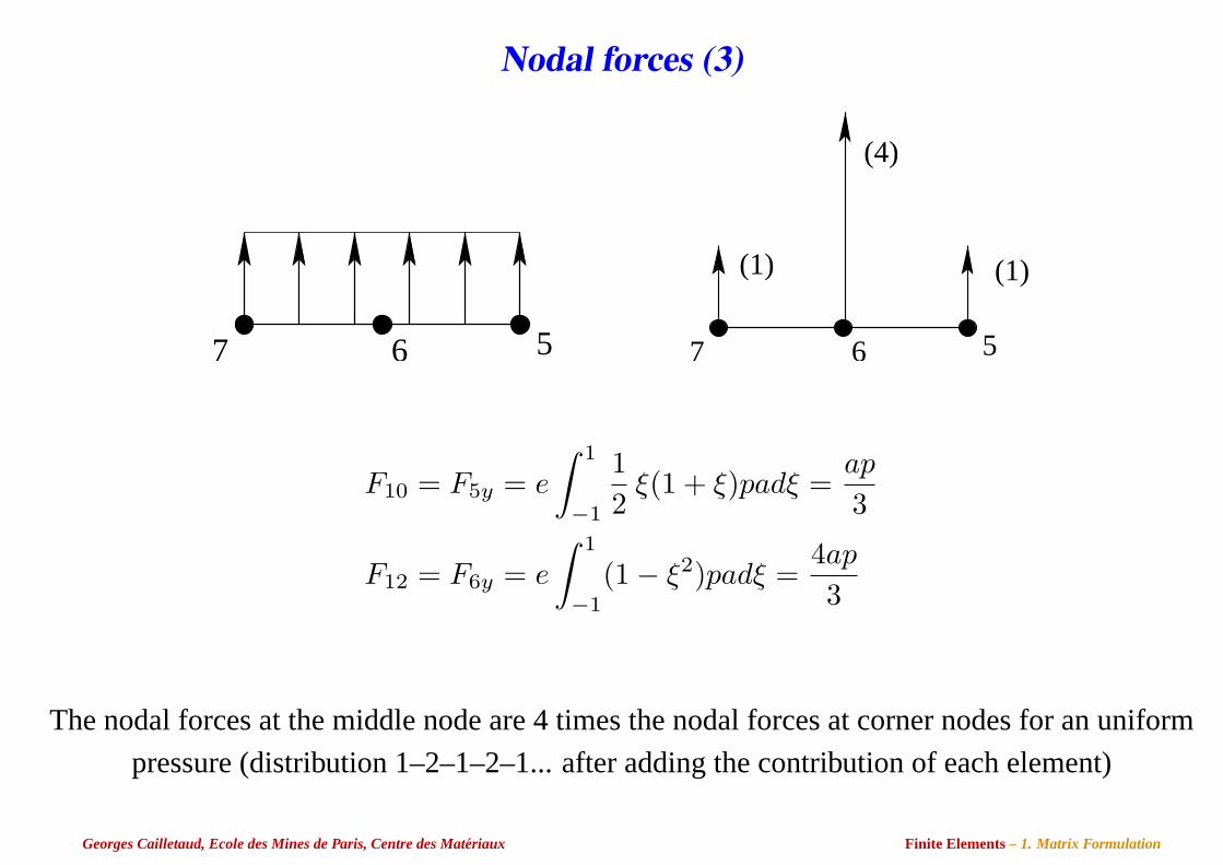
Nodal forces (3)
7 6 5 7 6 5
(1)
(4)
(1)
F10 = F5y = e
∫ 1
−1
12
ξ(1 + ξ)padξ =ap
3
F12 = F6y = e
∫ 1
−1
(1− ξ2)padξ =4ap
3
The nodal forces at the middle node are 4 times the nodal forces at corner nodes for an uniform
pressure (distribution 1–2–1–2–1... after adding the contribution of each element)
Georges Cailletaud, Ecole des Mines de Paris, Centre des Materiaux Finite Elements– 1. Matrix Formulation
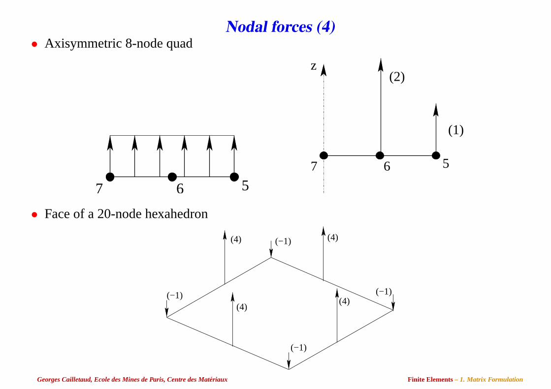
Nodal forces (4)• Axisymmetric 8-node quad
7 6 57 6 5
(2)
(1)
z
• Face of a 20-node hexahedron
(4)
(4)
(4)
(4)
(−1)
(−1)
(−1)
(−1)
Georges Cailletaud, Ecole des Mines de Paris, Centre des Materiaux Finite Elements– 1. Matrix Formulation
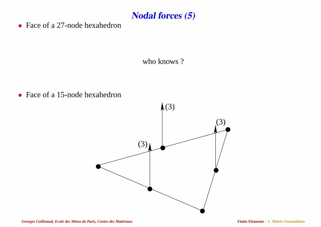
Nodal forces (5)• Face of a 27-node hexahedron
who knows ?
• Face of a 15-node hexahedron
(3)
(3)
(3)
Georges Cailletaud, Ecole des Mines de Paris, Centre des Materiaux Finite Elements– 1. Matrix Formulation
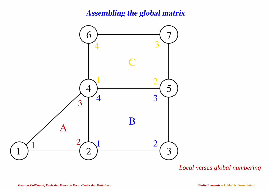
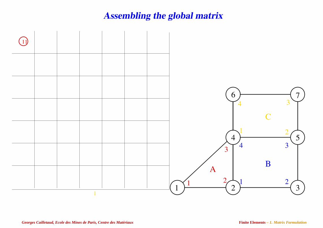
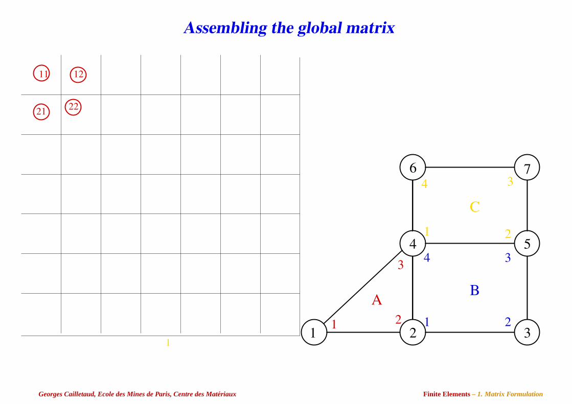
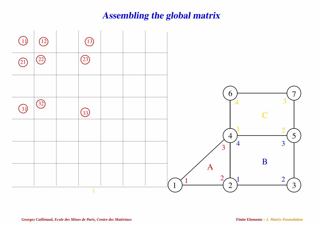
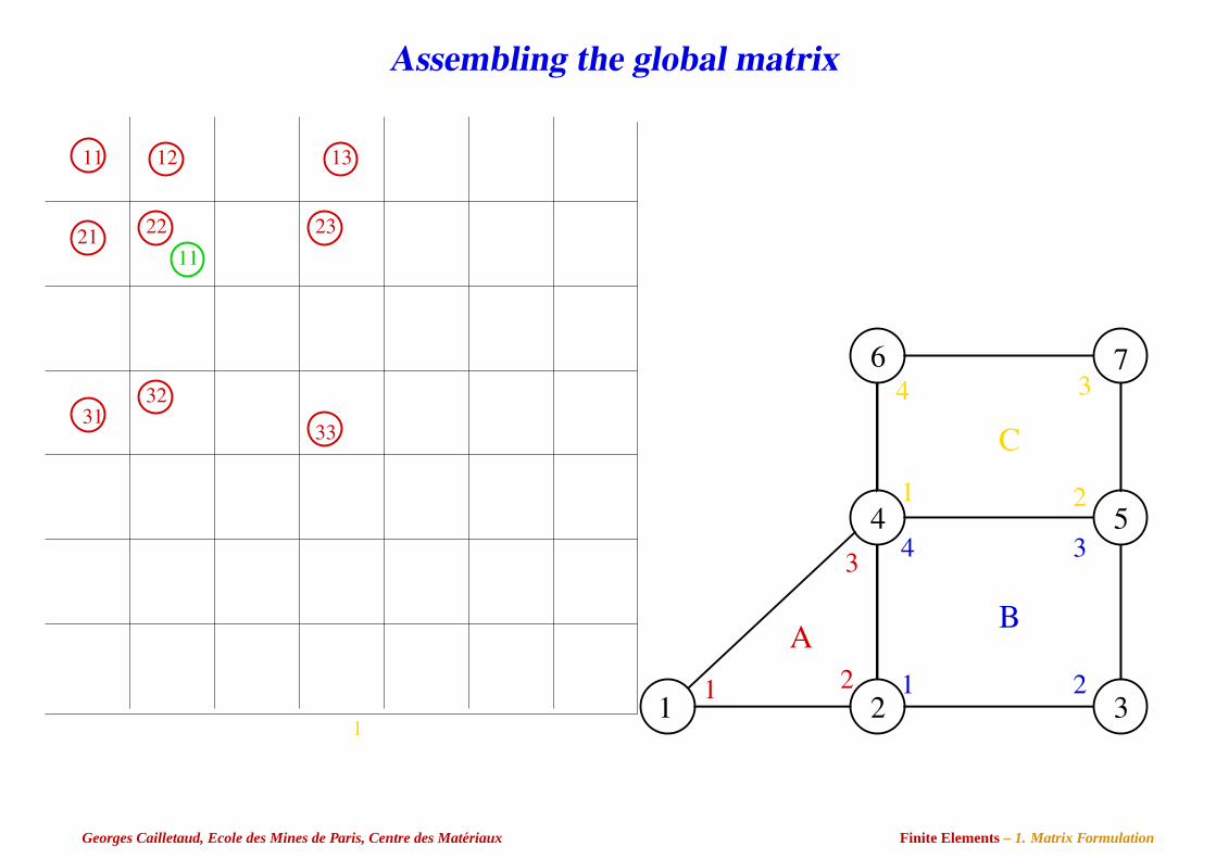
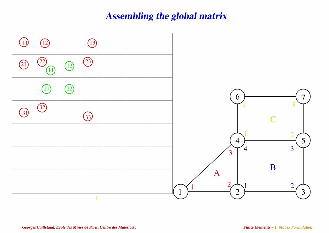
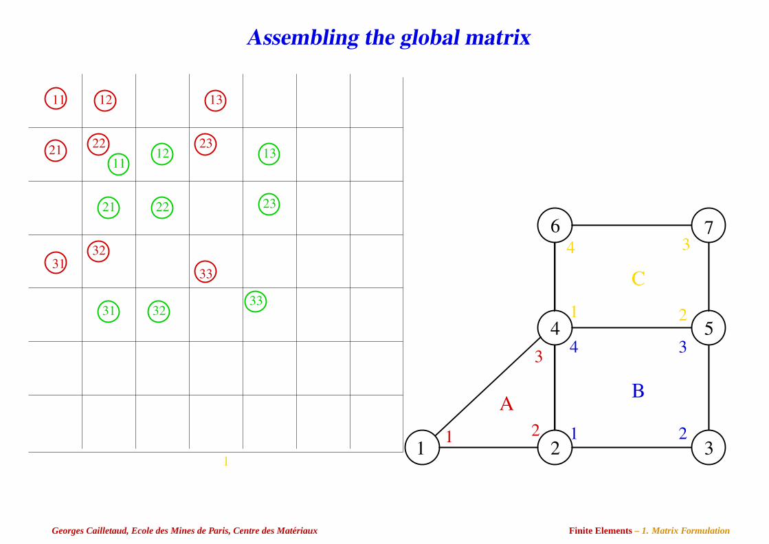
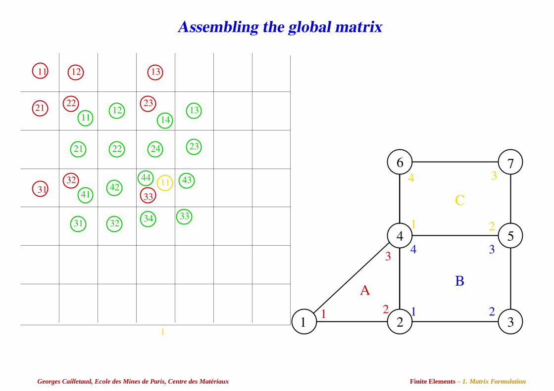
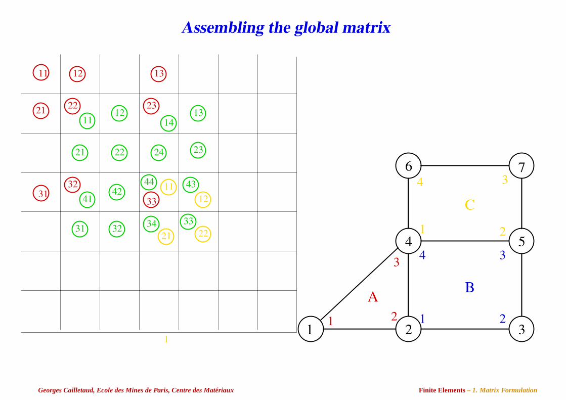
Assembling the global matrix
2 3
4 5
7
1
6
AB
1 1
1
2 2
3 3
3
4
4
C
2
Localversusglobal numbering
Georges Cailletaud, Ecole des Mines de Paris, Centre des Materiaux Finite Elements– 1. Matrix Formulation
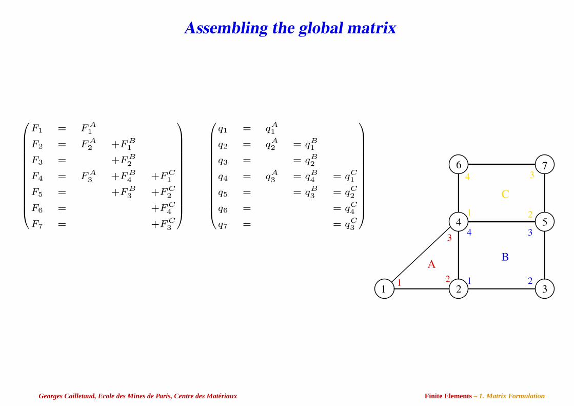
Assembling the global matrix
F1 = F A1
F2 = F A2 +F B
1
F3 = +F B2
F4 = F A3 +F B
4 +F C1
F5 = +F B3 +F C
2
F6 = +F C4
F7 = +F C3
q1 = qA1
q2 = qA2 = qB
1
q3 = = qB2
q4 = qA3 = qB
4 = qC1
q5 = = qB3 = qC
2
q6 = = qC4
q7 = = qC3
2 3
4 5
7
1
6
AB
1 1
1
2 2
3 3
3
4
4
C
2
Georges Cailletaud, Ecole des Mines de Paris, Centre des Materiaux Finite Elements– 1. Matrix Formulation
Assembling the global matrix
11
12 3
4 5
7
1
6
AB
1 1
1
2 2
3 3
3
4
4
C
2
Georges Cailletaud, Ecole des Mines de Paris, Centre des Materiaux Finite Elements– 1. Matrix Formulation
Assembling the global matrix
21
11 12
22
12 3
4 5
7
1
6
AB
1 1
1
2 2
3 3
3
4
4
C
2
Georges Cailletaud, Ecole des Mines de Paris, Centre des Materiaux Finite Elements– 1. Matrix Formulation
Assembling the global matrix
21
11 12 13
22 23
3231
33
12 3
4 5
7
1
6
AB
1 1
1
2 2
3 3
3
4
4
C
2
Georges Cailletaud, Ecole des Mines de Paris, Centre des Materiaux Finite Elements– 1. Matrix Formulation

Assembling the global matrix
21
11 12 13
1122 23
3231
33
12 3
4 5
7
1
6
AB
1 1
1
2 2
3 3
3
4
4
C
2
Georges Cailletaud, Ecole des Mines de Paris, Centre des Materiaux Finite Elements– 1. Matrix Formulation
Assembling the global matrix
21
11 12 13
1122 23
3231
33
12 3
4 5
7
1
6
AB
1 1
1
2 2
3 3
3
4
4
C
2
Georges Cailletaud, Ecole des Mines de Paris, Centre des Materiaux Finite Elements– 1. Matrix Formulation
Assembling the global matrix
21
11 12 13
1122
1223
2221
3231
33
12 3
4 5
7
1
6
AB
1 1
1
2 2
3 3
3
4
4
C
2
Georges Cailletaud, Ecole des Mines de Paris, Centre des Materiaux Finite Elements– 1. Matrix Formulation
Assembling the global matrix
33
21
11 12 13
1122
1223
13
232221
3231
31 32
33
12 3
4 5
7
1
6
AB
1 1
1
2 2
3 3
3
4
4
C
2
Georges Cailletaud, Ecole des Mines de Paris, Centre des Materiaux Finite Elements– 1. Matrix Formulation
Assembling the global matrix
44
33
1133
43
34
21
11 12 13
1122
1214
2313
23242221
4132
31
31 32
42
12 3
4 5
7
1
6
AB
1 1
1
2 2
3 3
3
4
4
C
2
Georges Cailletaud, Ecole des Mines de Paris, Centre des Materiaux Finite Elements– 1. Matrix Formulation
Assembling the global matrix
44
33
1133
22
12
21
43
34
21
11 12 13
1122
1214
2313
23242221
4132
31
31 32
42
12 3
4 5
7
1
6
AB
1 1
1
2 2
3 3
3
4
4
C
2
Georges Cailletaud, Ecole des Mines de Paris, Centre des Materiaux Finite Elements– 1. Matrix Formulation
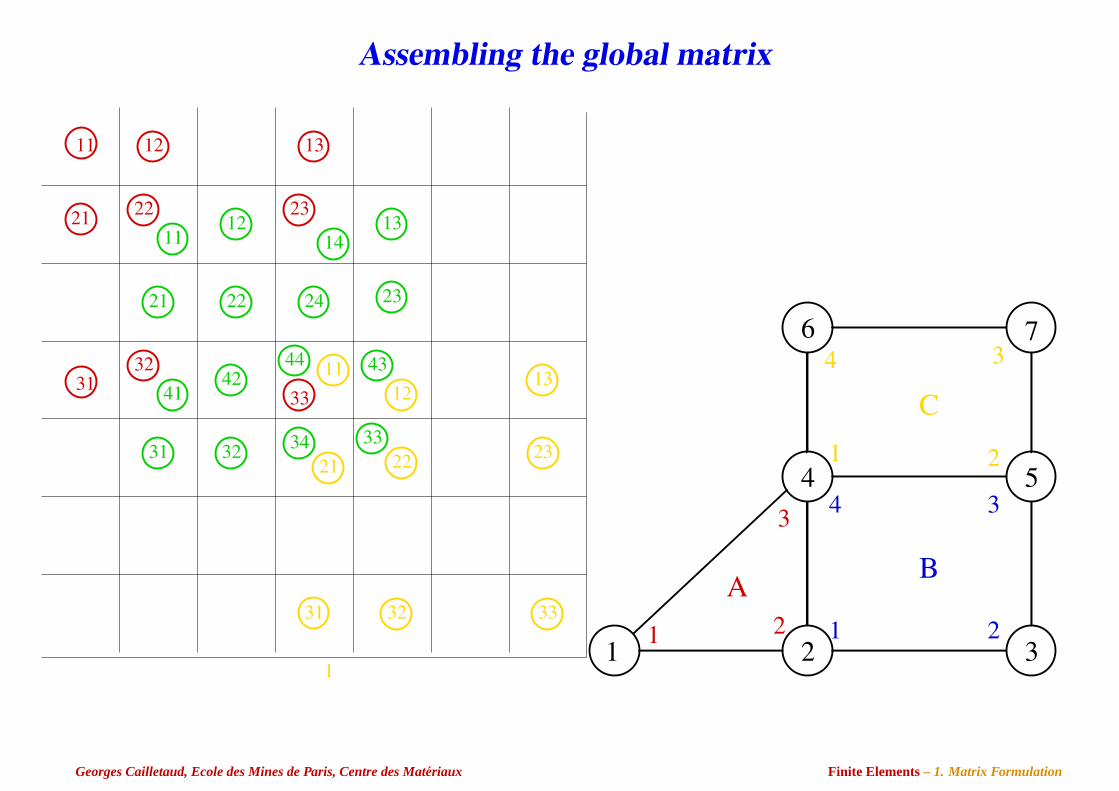
Assembling the global matrix
44
33
1133
22
12
21
43
34 23
13
31
21
11 12 13
1122
1214
2313
23242221
4132
31
31 32
42
32 33
12 3
4 5
7
1
6
AB
1 1
1
2 2
3 3
3
4
4
C
2
Georges Cailletaud, Ecole des Mines de Paris, Centre des Materiaux Finite Elements– 1. Matrix Formulation
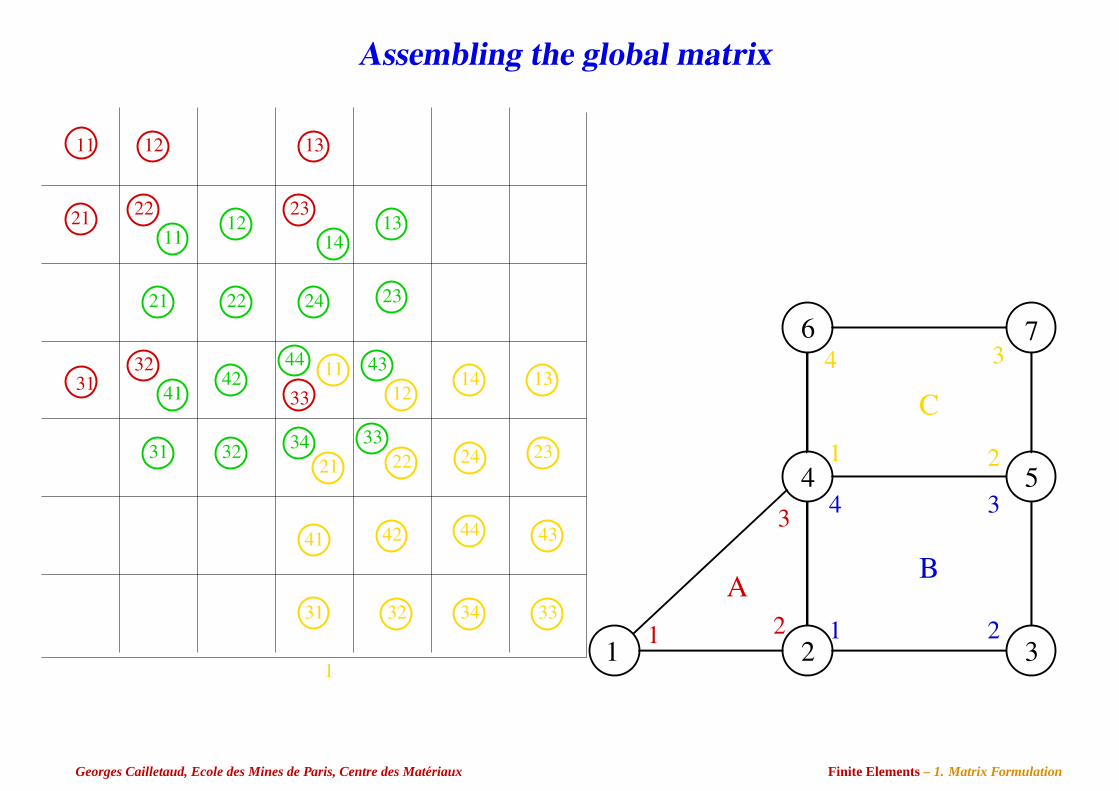
Assembling the global matrix
44
33
1133
22
12
21
43
34 23
13
31
21
11 12 13
1122
1214
2313
23242221
4132
31
31 32
42 14
43444241
3432 33
24
12 3
4 5
7
1
6
AB
1 1
1
2 2
3 3
3
4
4
C
2
Georges Cailletaud, Ecole des Mines de Paris, Centre des Materiaux Finite Elements– 1. Matrix Formulation
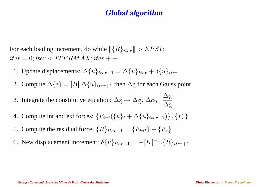
Global algorithm
For each loading increment, do while‖Riter‖ > EPSI:
iter = 0; iter < ITERMAX; iter + +
1. Update displacements:∆uiter+1 = ∆uiter + δuiter
2. Compute∆ε = [B].∆uiter+1 then∆ε∼ for each Gauss point
3. Integrate the constitutive equation:∆ε∼→ ∆σ∼, ∆αI ,∆σ∼∆ε∼
4. Compute int and ext forces:Fint(ut + ∆uiter+1) , Fe
5. Compute the residual force:Riter+1 = Fint − Fe
6. New displacement increment:δuiter+1 = −[K]−1.Riter+1
Georges Cailletaud, Ecole des Mines de Paris, Centre des Materiaux Finite Elements– 1. Matrix Formulation
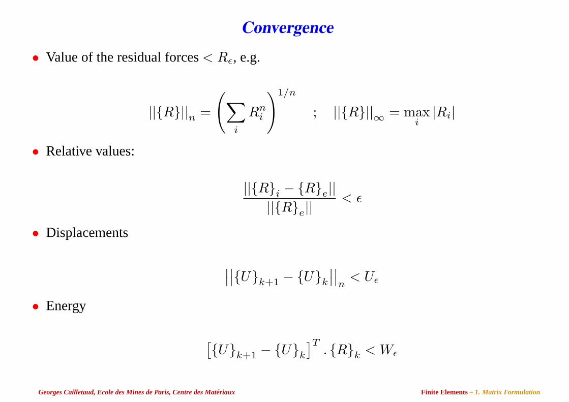
Convergence
• Value of the residual forces< Rε, e.g.
||R||n =
(∑i
Rni
)1/n
; ||R||∞ = maxi|Ri|
• Relative values:
||Ri − Re||||Re||
< ε
• Displacements
∣∣∣∣Uk+1 − Uk
∣∣∣∣n
< Uε
• Energy
[Uk+1 − Uk
]T. Rk < Wε
Georges Cailletaud, Ecole des Mines de Paris, Centre des Materiaux Finite Elements– 1. Matrix Formulation