GRC Transactions, Vol. 36, 2012

121

KeywordsGeothermal, Nevada, production wells, power plants, drilling costs, well depths, cost per MW

ABSTRACT

Expected well costs can be a major factor in whether compa-nies obtain financing due to expense and moderate success rates of drilling. Well permitting records are reported by state agencies, and well production from indi-vidual wells within producing areas are reported monthly (in NV) so that one can determine, in retrospect, which of the permitted wells actually led to geothermal production and power generation. A companion paper (Shevenell, 2012, this volume) compiles and evaluates geothermal well records submitted to the Nevada Division of Minerals, and estimates the success rates of geothermal wells drilled in Nevada since the early stages of exploration in the 1970s and 1980s, through construction of the power plants currently in existence in northern Nevada. This paper uses that informa-tion to estimate the minimum expected costs associated with drilled wells and production per MW, assuming well depths are a dominant factor in determining costs. Because depths are not the only factor determining power plant costs, costs noted here are likely minima.

Introduction

This paper uses well records compiled by the Nevada Divi-sion of Minerals to estimate the range of drilling costs for Nevada geothermal wells. The well depth data are available from the early stages of exploration in the 1970s and 1980s, through construction of the power plants and are used to calculate total and average well depths and associated minimum costs by producing area. It is com-mon to hear comments related to the “success rate” of geothermal

The Estimated Costs as a Function of Depth of Geothermal Development Wells Drilled in Nevada

Lisa Shevenell

ATLAS Geosciences Inc. and Nevada Bureau of Mines and Geology, Reno, NVlisas@atlasgeoinc.com

Figure 1. Location of existing and planned power plants in Nevada. Steamboat-binary consists of 6 separate power plant units that have a combined generating capacity of 137 MW. Only the three new plants constructed since 1992 are listed separately under the binary category.

122

Shevenell

wells in the context of overall development costs and financing, with numbers on the order of 50-75% commonly used to estimate the success rate (typically in reference to production wells). These assertions are often in the context that individual production wells are on the order of $3-5 million, with the implication that even unsuccessful wells could cost a developer up to $5 million. Such risk-benefit scenarios may be difficult to sell to investors, certainly if the first few wells drilled fall into this category. As reported by Hance (2005) “… debt lenders (commercial banks) will also require 25% of the resource capacity to be proven before lending any money. This means that all early phases of the project have to be financed by equity. The actual cost of these phases rises quickly as time goes on. Up-to-date cost information is often site-specific and tends to be held proprietary by researchers and consultants. … few articles thus address geothermal development costs in a comprehensive way and those tend to be based on outdated data.”

Given the paucity of reliable cost data, this paper attempts to determine the relative costs of geothermal well drilling us-ing publicly-available data and empirically-derived cost-depth relationships. All drilled wells are considered in this analysis, including preliminary and exploratory wells, because each helps define an individual resource, which, in turn, should help increase the success rates of future wells drilled for production and injec-tion. Hence, the costs of the preliminary and exploratory wells need to be considered in evaluations of power generation field expenses. Well completion data are available from the Nevada Division of Minerals (DOM) for the nine currently producing power plant areas (that may include one or more commercial units each) in Nevada using available data through 2010 (e.g., more than nine areas are producing, but the more recently constructed power plants do not yet have sufficient data for evaluation). These data are currently being compiled and quality checked for inclusion into the National Geothermal Data System (NGDS) to be made publicly and freely available through several user interfaces.

Background

Figure 1 shows the locations of the operating and planned power plants in Nevada as of mid-2012 showing current name-plate capacity.

A brief description of each of the new power plants constructed since 1992 and the relationship between the number of permits and drilled wells can be found in Shevenell and Zehner (2011) and Shevenell (2012, this volume). Earlier descriptions are found in Garside et al. (2002) and in the annual Nevada Mineral Industry reports (http://www.nbmg.unr.edu/dox/mi/XX.pdf, where XX are the last two digits of the individual year from this annual report series, which was first published in 1979 for 1978 information).

Methods

An overall summary of results from all sites is pro-vided, and a comparison of site observations appears in Shevenell (2012; this volume) for numbers of wells and depth, depth drilled per MW, and number of wells drilled per MW. Permitted domestic wells are excluded from the analysis since few currently-producing power

plant areas have nearby and are not relevant to the analysis here. Two time periods were evaluated for each producing plant in Shevenell (2012): pre-commissioning (including all wells permit-ted for exploration up to and including plant construction), and post-commissioning (including wells drilled to better define and expand the resource). The pre-commissioning data are presented here, based on results in Shevenell (2012), because these have the most complete depth data. Many depths (up to 53%, average of 35%, Table 5 of Shevenell (2012)) are missing from the post-commissioning well records, making it an unreliable data set for cost evaluations predicated on depth. Datasets for each power producing operation (Steamboat being considered as one area/operation) are evaluated to determine the costs of wells drilled. Drilling depth and cost data were compiled from the published literature and one well in NV for determination of cost estimates using empirically determined relationships with depth determined with data reported by Hance (2004), Augustine et al. (2006), Mansure (2005) and unpublished data from one well drilled at Bradys, NV, which has detailed cost by foot of penetration data. Most data obtained from Augustine et al. (2006) were compiled from the Joint Association Survey on Drilling Costs (1976-2000) from oil and gas wells. Note that Bloomfield and Laney (2005) also report well drilling cost estimates, but mostly using the same data reported by GeothermEx (Klein et al., 2004), and are thus, not reported separately.

In each set of Results tables, the well costs are noted by geo-thermal field for average numbers and depths of wells per field. The wells investigated were subdivided as follows: E for Explora-tion, I for Injection, O for Observation and P for Production. In some cases the production and injection wells are lumped in the original data as Industrial wells, in which case those wells are assumed to be production wells. It is assumed that wells would have been labeled as injection if indeed they were because injec-tion well permitting requires a unique form distinct from the other permitted wells. The following were categorized as exploration wells: exploration, test, stratigraphic test, thermal gradient and geothermal wells.

All cost data from published historical and unpublished (Bradys) data sources were escalated to 2012 dollars using a calculator available on the US Bureau of Labor Statistics: http://data.bls.gov/cgi-bin/cpicalc.pl?cost1=500%2C000.00&year1=2003&year2=2010. All calculations and results are made using these adjustments to 2012 US dollars.

Table 1. Total feet drilled by area for production and injection wells.

# P # I #P+I P feet I feet ft (P+I) Ave ft P Ave ft IBeowawe 2 1 3 11,165 5,927 17,092 5,583 5,927Bradys 11 1 12 18,328 3,123 21,451 1,666 3,123Desert eak 3 1 4 13,465 3,192 16,657 4,488 3,192Dixie Valley 10 7 17 94,091 59,747 153,838 9,409 8,535San Emidio 3 2 5 1,423 1,106 2,529 474 553Soda Lake 1 1 2 8,489 4,306 12,795 8,489 4,306Steamboat 13 2 15 15,587 4,321 19,908 1,199 2,161Stillwater 4 1 5 8,173 2,920 11,093 2,043 2,920Wabuska 1 3 4 500 2,460 2,960 500 820 Average 5.3 2.1 7.4 19,025 9,678 28,703 3,761 3,504 Stdev 4.7 2.0 5.6 28,770 18,824 47,407 3,418 2,503

123

Shevenell

ResultsGeneral Summary

Because Steamboat has several different power plants, which often use wells interchangeably (either continuously or spo-radically), the Steamboat area is considered in total, and not by individual power plant unit. Numbers of wells and depths by well category appear in Table 1.

Depth data are considerably more complete for the pre-com-missioning set of wells than for the post commissioning wells. Only two wells had no reported depths: 1 exploration well at Desert Peak and one exploration well at Steamboat. Hence, general conclusions are not adversely impacted by lack of available data in the pre-commissioning data set.

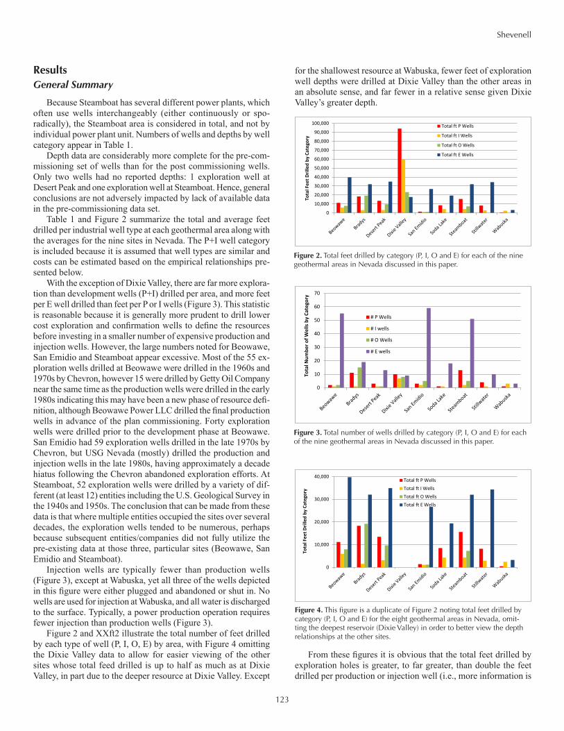
Table 1 and Figure 2 summarize the total and average feet drilled per industrial well type at each geothermal area along with the averages for the nine sites in Nevada. The P+I well category is included because it is assumed that well types are similar and costs can be estimated based on the empirical relationships pre-sented below.

With the exception of Dixie Valley, there are far more explora-tion than development wells (P+I) drilled per area, and more feet per E well drilled than feet per P or I wells (Figure 3). This statistic is reasonable because it is generally more prudent to drill lower cost exploration and confirmation wells to define the resources before investing in a smaller number of expensive production and injection wells. However, the large numbers noted for Beowawe, San Emidio and Steamboat appear excessive. Most of the 55 ex-ploration wells drilled at Beowawe were drilled in the 1960s and 1970s by Chevron, however 15 were drilled by Getty Oil Company near the same time as the production wells were drilled in the early 1980s indicating this may have been a new phase of resource defi-nition, although Beowawe Power LLC drilled the final production wells in advance of the plan commissioning. Forty exploration wells were drilled prior to the development phase at Beowawe. San Emidio had 59 exploration wells drilled in the late 1970s by Chevron, but USG Nevada (mostly) drilled the production and injection wells in the late 1980s, having approximately a decade hiatus following the Chevron abandoned exploration efforts. At Steamboat, 52 exploration wells were drilled by a variety of dif-ferent (at least 12) entities including the U.S. Geological Survey in the 1940s and 1950s. The conclusion that can be made from these data is that where multiple entities occupied the sites over several decades, the exploration wells tended to be numerous, perhaps because subsequent entities/companies did not fully utilize the pre-existing data at those three, particular sites (Beowawe, San Emidio and Steamboat).

Injection wells are typically fewer than production wells (Figure 3), except at Wabuska, yet all three of the wells depicted in this figure were either plugged and abandoned or shut in. No wells are used for injection at Wabuska, and all water is discharged to the surface. Typically, a power production operation requires fewer injection than production wells (Figure 3).

Figure 2 and XXft2 illustrate the total number of feet drilled by each type of well (P, I, O, E) by area, with Figure 4 omitting the Dixie Valley data to allow for easier viewing of the other sites whose total feed drilled is up to half as much as at Dixie Valley, in part due to the deeper resource at Dixie Valley. Except

for the shallowest resource at Wabuska, fewer feet of exploration well depths were drilled at Dixie Valley than the other areas in an absolute sense, and far fewer in a relative sense given Dixie Valley’s greater depth.

From these figures it is obvious that the total feet drilled by exploration holes is greater, to far greater, than double the feet drilled per production or injection well (i.e., more information is

0

10,000

20,000

30,000

40,000

50,000

60,000

70,000

80,000

90,000

100,000

Tota

l Fee

t Dril

led

by C

ateg

ory

Total ft P Wells

Total ft I Wells

Total ft O Wells

Total ft E Wells

0

10

20

30

40

50

60

70

Tota

l Num

ber o

f Wel

ls b

y Ca

tego

ry

# P Wells

# I wells

# O Wells

# E wells

0

10,000

20,000

30,000

40,000

Tota

l Fee

t Dril

led

by C

ateg

ory

Total ft P WellsTotal ft I WellsTotal ft O WellsTotal ft E Wells

Figure 2. Total feet drilled by category (P, I, O and E) for each of the nine geothermal areas in Nevada discussed in this paper.

Figure 3. Total number of wells drilled by category (P, I, O and E) for each of the nine geothermal areas in Nevada discussed in this paper.

Figure 4. This figure is a duplicate of Figure 2 noting total feet drilled by category (P, I, O and E) for the eight geothermal areas in Nevada, omit-ting the deepest reservoir (Dixie Valley) in order to better view the depth relationships at the other sites.

124

Shevenell

gathered more cheaply during earlier phase exploration using less expensive wells). The E wells are typically much less expensive ($15 per foot based on Klein et al., 2004; or $18.70/ft in 2012 dollars), and are reported separately. However, the author believes this estimate of cost per foot is likely to be too low in most cases where various complications can be expected. The O wells were often converted to a P or I well (15% of them) so the cost of those wells could be either closer to the $18.7/ft or the empirical costs depending on how the well was completed, which is typically not known. Hence, the P and I wells are the focus of the cost estimates of development but a hybrid estimate of the cost of the O wells is provided (assuming 15% of the feet cost $18.7/ft, and 85% cost the values calculated with the empirical relationships).

These average feet per well type in Table 2 multiplied by the number of wells per type per area are used below with the empirical relationships to estimate cost of wells used in production operations (P and I). “Success rates” of the various well types by geothermal area by depth and number are presented in Shevenell (2012).

RegressionsRegressions were calculated for the various datasets obtained

from the literature in various combinations to determine the best

fit for the available data. Data were plotted directly to test different models, but it was found that plots of the log(Cost $US) versus depth provided the best fit to the data. Augustine et al. (2006) also reported cost data as log values for the same reason. Table 3 lists results of assembled data sets and some combinations of model fits (exponential, linear, polynomial and power) using the log(Cost $US) versus depth relationships. Note that one set of data notes all data minus the values from Tester, which are largely based on data from the oil and gas industry, and are typically lower than those obtained in the plots showing geothermal well costs by depth from the other sources of information. The best R2 value for each data set is noted in bold in the table. Neither the exponential or linear models were the best fit for any of the data, although some showed good correlations with the data (Bradys, Mansure, and Augustine data). None of the R2 values are particularly good using the GeothermEx data (Klein et al. (2004)), although the power function best matches the complete data set. The power regression provided the best fit of the data for some of the data combinations, whereas the polynomial regression provided the best fit for the other combinations. Although the two model fits were typically fairly close to one another when comparing the R2 values, the equations for the models for the ones in bold were used in further analyses.

If the GeothermEx data are plotted by geo-graphic region, markedly different regression equations are obtained (Figure 5) due to the large scatter in data values. This plot illustrates that the GeothermEx R2 using all data is relatively low compared to other datasets.

Other variability is not explicitly accounted for in the data sets. For instance, the data presented by Mansure et al. (2005) show a distinct difference in costs from the 1970s to the 1980s (Figure 6), with costs shifting lower in the 1980s. Figure 6 shows the regression equation for the 1970s data set, which is similar to the full data set, although with a slightly better correlation coefficient (R2 = 0.909 versus 0.832). The equation for all Mansure data is

log ($ US - 2012) = 3.882(Depth)0.0558 R2 = 0.832

Table 2. The number of feet per well type drilled.

ft per P ft per I ft per E ft per OBeowawe 5,583 5,927 722 3,966Bradys 1,666 3,123 1,687 1,280Desert Peak 4,488 3,192 2,686 9,641Dixie Valley 9,409 8,535 1,970 2,906San Emidio 474 553 451 235Soda Lake 8,489 4,306 1,075 0Steamboat 1,199 2,161 628 1,453Stillwater 2,043 2,920 3,432 0Wabuska 500 820 1,081 0 Average 3,761 3,504 1,526 2,165 Stdev 3,418 2,503 1,013 3,138

Table 3. R2 values for four types of regression analyses noting the best fit for each data set in bold.

Exponential Linear Polynomial PowerAll Data 0.486 0.492 0.556 0.567All Data minus Tester 0.552 0.552 0.609 0.624Bradys 0.843 0.852 0.946 0.920GeothermEx Geysers 0.641 0.638 0.687 0.666GeothermEx El Salvador 0.418 0.418 0.433 0.432GeothermEx Other US 0.332 0.336 0.357 0.309GeothermEx All Data 0.442 0.444 0.473 0.514Mansure All 0.715 0.729 0.785 0.832Mansure 1970s 0.736 0.755 0.902 0.909Tester 1,800-10,000 ft 0.969 0.965 0.992 0.850Tester 1,800-20,000 ft 0.994 0.994 0.995 0.909

y = -2E-08x2 + 0.0004x + 4.4877 R² = 0.687

y = 3E-08x2 - 0.0002x + 6.7633 R² = 0.357

y = -6E-09x2 + 0.0001x + 6.0559 R² = 0.433

5.4

5.6

5.8

6.0

6.2

6.4

6.6

6.8

7.0

0 2,000 4,000 6,000 8,000 10,000 12,000 14,000

Log

(US

$ - 2

012)

Depth (feet)

The Geysers

Other US

El Salvador

Azores

Guatemala

Poly. (The Geysers)

Poly. (Other US)

Poly. (El Salvador)

Figure 5. Log Cost in dollars (2012) versus well depths for data reported in the GeothermEx Pier Report (Klein et al., 2004) by geographic area.

125

Shevenell

Similarly, there are other sources of variability in the data sets. Figure 7 plots the log costs versus well depth for all data compiled for this paper and shows that the Augustine data consistently pre-dict lower costs than the other data. The Augustine data is largely from oil and gas drilling results, whereas the other compiled data are for wells drilled for geothermal purposes. Hence, the Augus-tine data will provide a lower bound to well costs by depth for the geothermal wells investigated here.

The best fit power function of all data plotted in Figure 7 islog (US$-2012) = 3.5077 (Depth)0.0679 R2 = 0.5673

The R2 is relatively low when all data are used in the regres-sion analysis due to significant data scatter as a result of variations in timing and location of data collection. Because of the scatter, three different regressions are used to estimate costs of production wells at the Nevada geothermal areas to provide a range of costs possible. As noted, the Augustine costs are likely too low, and the Bradys costs are only from one well, but are likely representative of the types of conditions drilled in Nevada geothermal areas. The Klein data are from multiple locations, some of which are close to the Bradys values, but most indicate higher costs.

The Augustine et al. (2006) best fit polynomial for the data isLog (Cost US-2012) = 4E-09D2 + 5E-05D + 5.3262 - R² =

0.994

The Klein et al. (2004) best fit power equation for the pre-sented data is

Log (Cost US-2012) = 4.0883D0.0531 - R² = 0.514

The Bradys (unpublished) best fit power equation for the data from one well during which cumulative costs were recorded is

Log (Cost US-2012) = 3.988D0.0485 - R² = 0.920

where D is well depth.Note that the Augustine data fit is best because the data were

smoothed by averaging depths over specific depth intervals (Figure 8).

Klein et al. (2004) developed the following function from sta-tistical analyses of historical drilling costs, showing that the depth of the well is a major (although not only) parameter explaining a well’s overall cost:

Drilling cost (in US$) = 240,785 + 210 x (depth in feet) + 0.019069 x (depth in feet), R2

= 0.558.

Hence, a significant portion of the cost variability of geother-mal wells evaluated in their study can be attributed to well depth. Of course, actual costs of wells may vary significantly from this due to a variety of other factors such as diameter, lost circulation, rock structure, hardness, and permeability, etc. (Hance, 2005). For the purposes of the current work in Nevada and comparisons (or minimum average costs) among sites, the three depth relationships (using log(Costs)) are used to estimate costs as a function of depth because depth is the only factor available from the evaluated data set and the regressions appear to match the data better than the relationship reported by Klein et al. (2004). All estimated costs are minima because factors impacting costs other than depth (material cost variability, dates of drilling, penetration rates, diameter, site assessments, etc.) are not considered here.

Estimated Well Costs Well costs are estimated using the three regression equations

noted in the previous section for Augustine, Bradys, and Klein

y = 3.6887x0.0625 R² = 0.909

5.6

5.8

6.0

6.2

6.4

6.6

6.8

0 2000 4000 6000 8000 10000 12000 14000 16000 18000

Log

($ U

S - 2

012)

Well Depth (feet)

1970s

1980s

Power (1970s)

Figure 6. Plot of well depths versus costs summarized from Mansure et al. (2006) illustrating the difference in costs between the 1970s and 1980s data, with the regression equation noted being for the 1970s data.

5.0

5.5

6.0

6.5

7.0

7.5

0 5000 10000 15000 20000

Log(

Cost

- U

S $

in 2

012)

Depth (feet)

Augustine

Klein

Bradys

Mansure

Figure 7. Plot of log costs versus well depth for all data compiled for this paper.

y = 4.0883x0.0531 R² = 0.514

y = 3.9888x0.0485 R² = 0.920

y = 4E-09x2 + 5E-05x + 5.3262 R² = 0.994

5.0

5.2

5.4

5.6

5.8

6.0

6.2

6.4

6.6

6.8

7.0

0 2000 4000 6000 8000 10000 12000 14000

Log

($ U

S - 2

012)

Well Depth (feet)

Klein

Bradys

Augustine

Power (Klein)

Power (Bradys)

Poly. (Augustine)

Figure 8. Plot showing three possible equations to calculate costs of pro-duction wells by depth.

126

Shevenell

(Table 4). This table lists the estimated cost by the three methods for both P and I wells separated, using the average depth of either the P or I wells at each site in Nevada resulting in an estimate of per well cost of industrial (P and I) wells. Dixie Valley is the most expen-sive to drill given its greater depth than the other reservoirs. However, other factors impact the estimated costs in Table 4 such as success rate because the calculations use average depths of either P or I drilled at each site, with-out consideration of which ones were actually used. The calculations were done in this manner to estimate the total project cost because some wells at these areas are either not successful or not used in the ultimate gen-eration facility, yet the costs for drilling them were still incurred. See Shevenell (2012, this volume) for success of wells drilled at these sites (i.e., how many were actually used per total depths drilled).

Table 5 lists the estimated costs per indus-trial well per project multiplying the numbers noted in Table 4 by the number of the P or I wells drilled at the site (whether they are used or not in the production operation).

Costs for the four major categories of wells drilled at each site are noted in Table 6, with the P and I costs using the average of the three regression equations and the average well depth multiplied by the total number of the wells per category drilled at each area. The E costs are likely low and used the $18.70 per foot (Klein et al., 2004) value to estimate costs of drilling the total depths of all E wells at each site. The costs of the observation (O) wells are a hybrid of the previous two calculations. Approximately 10% of the wells initially drilled as observation wells were converted to P or I wells after drilling (Shevenell 2012, this volume). Therefore, an estimate of costs for these O wells was obtained by calculating the average regression equation values used for P and I multiplied by 20%, with 90% of the noted cost being that of an E well. Other estimates could be made because well diameter is not one of the data values avail-able in this work, and that would be useful to better determine which category the drilled O wells fit into relative to being either an industrial or exploration well. Table 6 also lists total estimated drilling costs for P, I, O and E by geothermal area, adjusted to 2012 dollars. These values do not include geologic, geochemical, or geophysical surveys and resource assessment work required to site the wells.

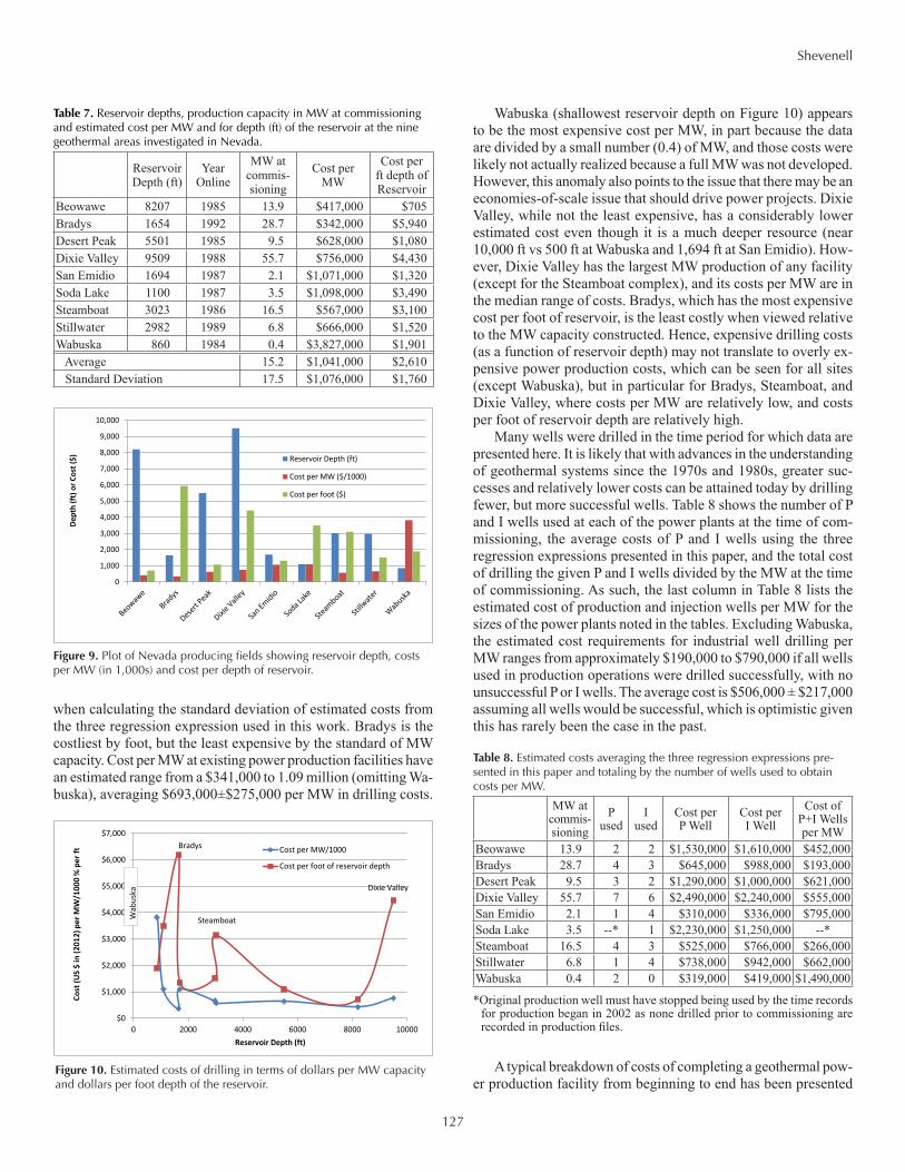
An important statistic is how much is the expected cost per MW of power produced, which is estimated for the nine sites in Nevada in Table 7, along with the estimated cost per foot depth of reservoir. These data are also plotted on Figure 9. Although Dixie

Valley produces from the deepest reservoir, it was neither costli-est from the perspective of depth nor number of MW produced (Figure 9). Beowawe, which produces from the next deepest reservoir, was one of the least costly to drill when considering both reservoir depth and numbers of MW produced.

Discussion

Costs per depth and MW are plotted by increasing order of cost in Table XXCostDis. Error bars are not shown to avoid clutter, but they are fairly large ranging from 40 to 80% for the P wells (average =66%) and 48 to 80% for the I wells (average = 72%)

Table 4. Average cost per well at each site using the three regression equations for P and I wells.

Augustine Bradys Klein Augustine Bradys KleinCost per Ave Cost per Ave Cost per Ave Cost per Ave Cost per Ave Cost per AveP well drilled P well drilled P well drilled I well drilled I well drilled I well drilled

Beowawe $537,000 $1,151,000 $2,907,000 $580,000 $1,200,000 $3,048,000Bradys $263,000 $520,000 $1,152,000 $332,000 $781,000 $1,850,000Desert Peak $428,000 $994,000 $245,000 $336,000 $793,000 $1,880,000Dixie Valley $1,415,000 $1,647,000 $4,417,000 $1,108,000 $1,539,000 $4,082,000San Emidio $224,000 $239,000 $468,000 $227,000 $262,000 $521,000Soda Lake $1,094,000 $1,534,000 $4,064,000 $413,000 $967,000 $2,371,000Steamboat $247,000 $422,000 $905,000 $284,000 $615,000 $1,400,000Stillwater $279,000 $593,000 $1,341,000 $321,000 $748,000 $1,760,000Wabuska $225,000 $247,000 $486,000 $234,000 $333,000 $688,000

Table 5. Total cost per area using the three regression equations for P and I wells by multiplying the total number of wells by the per well costs in Table 4.

Augustine Bradys Klein Augustine Bradys KleinTotal Cost Total Cost Total Cost Total Cost Total Cost Total Cost

P Wells P Wells P Wells I Wells I Wells I WellsBeowawe $1,074,000 $2,303,000 $5,815,000 $580,000 $1,200,000 $3,048,000Bradys $2,897,000 $5,721,000 $12,680,000 $332,000 $781,000 $1,850,000Desert Peak $1,283,000 $2,983,000 $7,348,000 $336,000 $793,000 $1,881,000Dixie Valley $14,150,000 $16,470,000 $44,175,000 $7,753,000 $10,780,000 $28,570,000San Emidio $673,000 $717,000 $1,404,000 $453,000 $524,000 $1,042,000Soda Lake $1,094,000 $1,534,000 $4,064,000 $413,000 $967,000 $2,371,000Steamboat $3,205,000 $5,489,000 $11,760,000 $567,000 $1,230,000 $2,798,000Stillwater $1,115,000 $2,371,000 $5,365,000 $321,000 $748,000 $1,757,000Wabuska $225,000 $247,000 $486,000 $703,000 $1,000,000 $2,064,000

Table 6. Estimated cost of all P, I, E and O wells drilled by area along with total drilling costs for the area (cost per well times number of wells per area are presented in this table). Average of the Klein, Augustine and Bradys values by well type by area are presented for P and I.

Costs P Costs I Costs E Costs O* Total Drilling Costs

Beowawe $3,064,000 $1,610,000 $743,000 $369,000 $5,790,000Bradys $7,100,000 $988,000 $599,000 $1,140,000 $9,830,000Desert Peak $3,870,000 $1,003,000 $653,000 $419,000 $5,950,000Dixie Valley $24,900,000 $15,700,000 $332,000 $1,140,000 $42,100,000San Emidio $931,000 $673,000 $498,000 $131,000 $2,230,000Soda Lake $2,230,000 $1,250,000 $362,000 $0 $3,840,000Steamboat $6,820,000 $1,530,000 $599,000 $418,000 $9,370,000Stillwater $2,950,000 $942,000 $642,000 $0 $4,530,000Wabuska $319,000 $1,260,000 $61,000 $0 $1,640,000

* O costs are calculated at 15% of P based on depth + 85% of E costs per foot

127

Shevenell

when calculating the standard deviation of estimated costs from the three regression expression used in this work. Bradys is the costliest by foot, but the least expensive by the standard of MW capacity. Cost per MW at existing power production facilities have an estimated range from a $341,000 to 1.09 million (omitting Wa-buska), averaging $693,000±$275,000 per MW in drilling costs.

Wabuska (shallowest reservoir depth on Figure 10) appears to be the most expensive cost per MW, in part because the data are divided by a small number (0.4) of MW, and those costs were likely not actually realized because a full MW was not developed. However, this anomaly also points to the issue that there may be an economies-of-scale issue that should drive power projects. Dixie Valley, while not the least expensive, has a considerably lower estimated cost even though it is a much deeper resource (near 10,000 ft vs 500 ft at Wabuska and 1,694 ft at San Emidio). How-ever, Dixie Valley has the largest MW production of any facility (except for the Steamboat complex), and its costs per MW are in the median range of costs. Bradys, which has the most expensive cost per foot of reservoir, is the least costly when viewed relative to the MW capacity constructed. Hence, expensive drilling costs (as a function of reservoir depth) may not translate to overly ex-pensive power production costs, which can be seen for all sites (except Wabuska), but in particular for Bradys, Steamboat, and Dixie Valley, where costs per MW are relatively low, and costs per foot of reservoir depth are relatively high.

Many wells were drilled in the time period for which data are presented here. It is likely that with advances in the understanding of geothermal systems since the 1970s and 1980s, greater suc-cesses and relatively lower costs can be attained today by drilling fewer, but more successful wells. Table 8 shows the number of P and I wells used at each of the power plants at the time of com-missioning, the average costs of P and I wells using the three regression expressions presented in this paper, and the total cost of drilling the given P and I wells divided by the MW at the time of commissioning. As such, the last column in Table 8 lists the estimated cost of production and injection wells per MW for the sizes of the power plants noted in the tables. Excluding Wabuska, the estimated cost requirements for industrial well drilling per MW ranges from approximately $190,000 to $790,000 if all wells used in production operations were drilled successfully, with no unsuccessful P or I wells. The average cost is $506,000 ± $217,000 assuming all wells would be successful, which is optimistic given this has rarely been the case in the past.

A typical breakdown of costs of completing a geothermal pow-er production facility from beginning to end has been presented

Table 7. Reservoir depths, production capacity in MW at commissioning and estimated cost per MW and for depth (ft) of the reservoir at the nine geothermal areas investigated in Nevada.

Reservoir Depth (ft)

Year Online

MW at commis-sioning

Cost per MW

Cost per ft depth of Reservoir

Beowawe 8207 1985 13.9 $417,000 $705Bradys 1654 1992 28.7 $342,000 $5,940Desert Peak 5501 1985 9.5 $628,000 $1,080Dixie Valley 9509 1988 55.7 $756,000 $4,430San Emidio 1694 1987 2.1 $1,071,000 $1,320Soda Lake 1100 1987 3.5 $1,098,000 $3,490Steamboat 3023 1986 16.5 $567,000 $3,100Stillwater 2982 1989 6.8 $666,000 $1,520Wabuska 860 1984 0.4 $3,827,000 $1,901 Average 15.2 $1,041,000 $2,610 Standard Deviation 17.5 $1,076,000 $1,760

0

1,000

2,000

3,000

4,000

5,000

6,000

7,000

8,000

9,000

10,000

Dept

h (ft

) or C

ost (

$)

Reservoir Depth (ft)

Cost per MW ($/1000)

Cost per foot ($)

Figure 9. Plot of Nevada producing fields showing reservoir depth, costs per MW (in 1,000s) and cost per depth of reservoir.

$0

$1,000

$2,000

$3,000

$4,000

$5,000

$6,000

$7,000

0 2000 4000 6000 8000 10000

Cost

(US

$ in

(201

2) p

er M

W/1

000

% p

er ft

Reservoir Depth (ft)

Cost per MW/1000

Cost per foot of reservoir depth

Bradys

Steamboat

Dixie Valley

Wab

uska

Figure 10. Estimated costs of drilling in terms of dollars per MW capacity and dollars per foot depth of the reservoir.

Table 8. Estimated costs averaging the three regression expressions pre-sented in this paper and totaling by the number of wells used to obtain costs per MW.

MW at commis-sioning

P used

I used

Cost per P Well

Cost per I Well

Cost of P+I Wells per MW

Beowawe 13.9 2 2 $1,530,000 $1,610,000 $452,000Bradys 28.7 4 3 $645,000 $988,000 $193,000Desert Peak 9.5 3 2 $1,290,000 $1,000,000 $621,000Dixie Valley 55.7 7 6 $2,490,000 $2,240,000 $555,000San Emidio 2.1 1 4 $310,000 $336,000 $795,000Soda Lake 3.5 --* 1 $2,230,000 $1,250,000 --*Steamboat 16.5 4 3 $525,000 $766,000 $266,000Stillwater 6.8 1 4 $738,000 $942,000 $662,000Wabuska 0.4 2 0 $319,000 $419,000 $1,490,000

*Original production well must have stopped being used by the time records for production began in 2002 as none drilled prior to commissioning are recorded in production files.

128

Shevenell

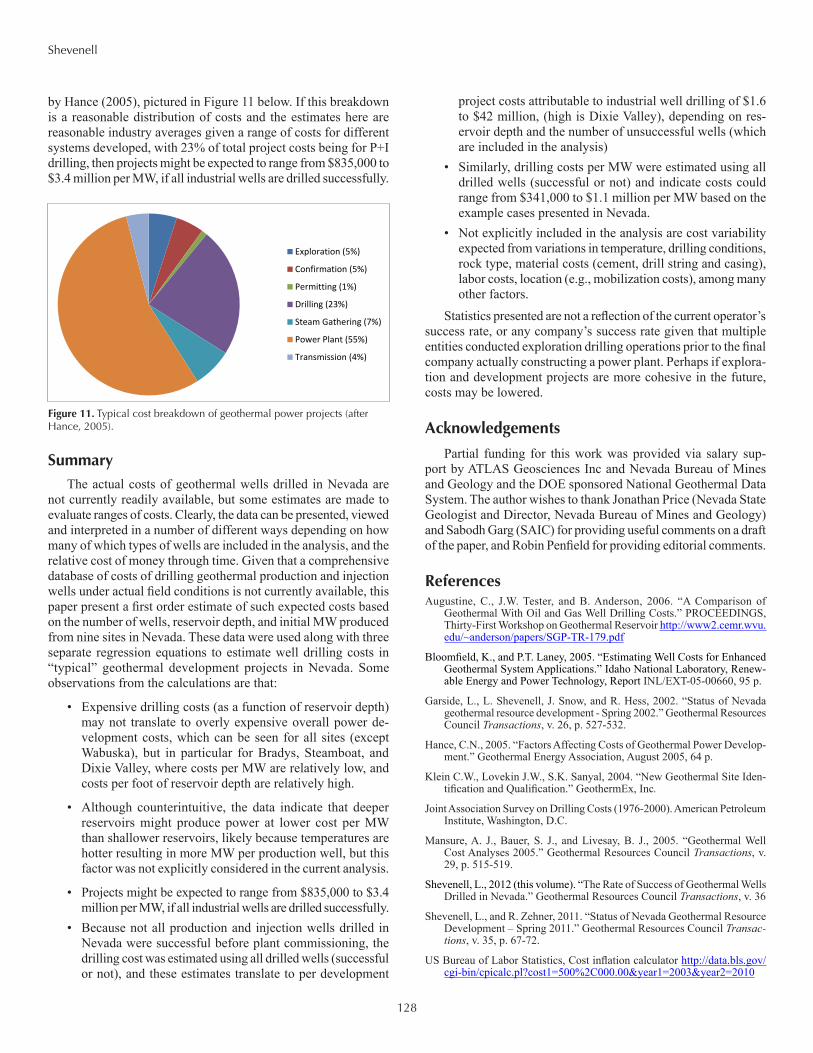
by Hance (2005), pictured in Figure 11 below. If this breakdown is a reasonable distribution of costs and the estimates here are reasonable industry averages given a range of costs for different systems developed, with 23% of total project costs being for P+I drilling, then projects might be expected to range from $835,000 to $3.4 million per MW, if all industrial wells are drilled successfully.

SummaryThe actual costs of geothermal wells drilled in Nevada are

not currently readily available, but some estimates are made to evaluate ranges of costs. Clearly, the data can be presented, viewed and interpreted in a number of different ways depending on how many of which types of wells are included in the analysis, and the relative cost of money through time. Given that a comprehensive database of costs of drilling geothermal production and injection wells under actual field conditions is not currently available, this paper present a first order estimate of such expected costs based on the number of wells, reservoir depth, and initial MW produced from nine sites in Nevada. These data were used along with three separate regression equations to estimate well drilling costs in “typical” geothermal development projects in Nevada. Some observations from the calculations are that:

• Expensive drilling costs (as a function of reservoir depth) may not translate to overly expensive overall power de-velopment costs, which can be seen for all sites (except Wabuska), but in particular for Bradys, Steamboat, and Dixie Valley, where costs per MW are relatively low, and costs per foot of reservoir depth are relatively high.

• Although counterintuitive, the data indicate that deeper reservoirs might produce power at lower cost per MW than shallower reservoirs, likely because temperatures are hotter resulting in more MW per production well, but this factor was not explicitly considered in the current analysis.

• Projects might be expected to range from $835,000 to $3.4 million per MW, if all industrial wells are drilled successfully.

• Because not all production and injection wells drilled in Nevada were successful before plant commissioning, the drilling cost was estimated using all drilled wells (successful or not), and these estimates translate to per development

project costs attributable to industrial well drilling of $1.6 to $42 million, (high is Dixie Valley), depending on res-ervoir depth and the number of unsuccessful wells (which are included in the analysis)

• Similarly, drilling costs per MW were estimated using all drilled wells (successful or not) and indicate costs could range from $341,000 to $1.1 million per MW based on the example cases presented in Nevada.

• Not explicitly included in the analysis are cost variability expected from variations in temperature, drilling conditions, rock type, material costs (cement, drill string and casing), labor costs, location (e.g., mobilization costs), among many other factors.

Statistics presented are not a reflection of the current operator’s success rate, or any company’s success rate given that multiple entities conducted exploration drilling operations prior to the final company actually constructing a power plant. Perhaps if explora-tion and development projects are more cohesive in the future, costs may be lowered.

Acknowledgements

Partial funding for this work was provided via salary sup-port by ATLAS Geosciences Inc and Nevada Bureau of Mines and Geology and the DOE sponsored National Geothermal Data System. The author wishes to thank Jonathan Price (Nevada State Geologist and Director, Nevada Bureau of Mines and Geology) and Sabodh Garg (SAIC) for providing useful comments on a draft of the paper, and Robin Penfield for providing editorial comments.

References Augustine, C., J.W. Tester, and B. Anderson, 2006. “A Comparison of

Geothermal With Oil and Gas Well Drilling Costs.” PROCEEDINGS, Thirty-First Workshop on Geothermal Reservoir http://www2.cemr.wvu.edu/~anderson/papers/SGP-TR-179.pdf

Bloomfield, K., and P.T. Laney, 2005. “Estimating Well Costs for Enhanced Geothermal System Applications.” Idaho National Laboratory, Renew-able Energy and Power Technology, Report INL/EXT-05-00660, 95 p.

Garside, L., L. Shevenell, J. Snow, and R. Hess, 2002. “Status of Nevada geothermal resource development - Spring 2002.” Geothermal Resources Council Transactions, v. 26, p. 527-532.

Hance, C.N., 2005. “Factors Affecting Costs of Geothermal Power Develop-ment.” Geothermal Energy Association, August 2005, 64 p.

Klein C.W., Lovekin J.W., S.K. Sanyal, 2004. “New Geothermal Site Iden-tification and Qualification.” GeothermEx, Inc.

Joint Association Survey on Drilling Costs (1976-2000). American Petroleum Institute, Washington, D.C.

Mansure, A. J., Bauer, S. J., and Livesay, B. J., 2005. “Geothermal Well Cost Analyses 2005.” Geothermal Resources Council Transactions, v. 29, p. 515-519.

Shevenell, L., 2012 (this volume). “The Rate of Success of Geothermal Wells Drilled in Nevada.” Geothermal Resources Council Transactions, v. 36

Shevenell, L., and R. Zehner, 2011. “Status of Nevada Geothermal Resource Development – Spring 2011.” Geothermal Resources Council Transac-tions, v. 35, p. 67-72.

US Bureau of Labor Statistics, Cost inflation calculator http://data.bls.gov/cgi-bin/cpicalc.pl?cost1=500%2C000.00&year1=2003&year2=2010

Exploration (5%)

Confirmation (5%)

Permitting (1%)

Drilling (23%)

Steam Gathering (7%)

Power Plant (55%)

Transmission (4%)

Figure 11. Typical cost breakdown of geothermal power projects (after Hance, 2005).