Embed Size (px)
Citation preview

JOURNAL OF FINANCIAL AND QUANTITATIVE ANALYSIS Vol. 46, No. 4, Aug. 2011, pp. 967–999COPYRIGHT 2011, MICHAEL G. FOSTER SCHOOL OF BUSINESS, UNIVERSITY OF WASHINGTON, SEATTLE, WA 98195doi:10.1017/S0022109011000275
The Effects of Derivatives on Firm Riskand Value
Sohnke M. Bartram, Gregory W. Brown, and Jennifer Conrad∗
Abstract
Using a large sample of nonfinancial firms from 47 countries, we examine the effect ofderivative use on firm risk and value. We control for endogeneity by matching users andnonusers on the basis of their propensity to use derivatives. We also use a new techniqueto estimate the effect of omitted variable bias on our inferences. We find strong evidencethat the use of financial derivatives reduces both total risk and systematic risk. The effectof derivative use on firm value is positive but more sensitive to endogeneity and omittedvariable concerns. However, using derivatives is associated with significantly higher value,abnormal returns, and larger profits during the economic downturn in 2001–2002, suggest-ing that firms are hedging downside risk.
I. Introduction
Derivatives are financial weapons of mass destruction.—Warren E. Buffett, 2003 Berkshire Hathaway Annual Report
The financial crisis of 2008–2009 has brought new scrutiny to the use offinancial derivatives. Recent proposals in major countries, including the UnitedStates, call for greater regulation of over-the-counter (OTC) derivatives, includ-ing conditions for marking positions to market prices, trade registration, tradeclearing, exchange trading, and higher capital and margin requirements.
∗Bartram, [email protected], Lancaster University, Management School, LancasterLA1 4YX, United Kingdom, and State Street Global Advisors; Brown, [email protected], Con-rad, j [email protected], Kenan-Flagler Business School, University of North Carolina at Chapel Hill,CB 3490, Chapel Hill, NC 27599. We thank Hendrik Bessembinder (the editor), Evgenia Golubeva,Reint Gropp, Peter Pope, Peter Tufano (the referee), Gautam Vora, Tracy Yue Wang, Chu Zhang,and seminar participants at the 2009 Meetings of the Western Finance Association, 18th Annual Con-ference on Financial Economics and Accounting, 2006 Financial Intermediation Research SocietyConference, 2007 Meetings of the Financial Management Association, DePaul University, ExeterUniversity, Florida State University, Georgia State University, Gottingen University, Hamburg Uni-versity, Manchester University, Munster University, Regensburg University, State Street Global Ad-visors, University of North Carolina at Chapel Hill, and York University for helpful comments andsuggestions. Financial support by the Leverhulme Trust is gratefully acknowledged. Bartram grate-fully acknowledges the warm hospitality of the Kenan-Flagler Business School of the University ofNorth Carolina, and the Red McCombs School of Business, University of Texas at Austin, duringvisits to these institutions.
967

968 Journal of Financial and Quantitative Analysis
The derivative securities that have caused the most harm during this eco-nomic downturn have been those held by financial firms. In contrast, there havebeen relatively few instances of problems with derivatives at nonfinancial firmsin the current downturn.1 As a consequence, in response to the proposed newregulations of derivatives, many nonfinancial firms in the U.S. (including energyproducers, airlines, and industrial equipment manufacturers) have started lobby-ing Congress, arguing that the proposed rule changes may “drive U.S. companiesto seek financing overseas, . . . [impair firms’ ability to] manage fluctuations inmaterials prices, commodities, fuel, interest rates, and foreign currency,” and, ingeneral, materially harm the 90% of Fortune 500 companies that use financialderivatives to manage risk.2
In fact, although data on derivatives usage have become available in the last2 decades, detailed empirical evidence on the effects of derivative use on firms’risk and value is still mixed. For example, using a sample of firms that initiatederivative use, Guay (1999) finds that the total risk, idiosyncratic risk, and risk ex-posures to interest rate changes of these firms decline, but he finds no significantchange in the market risk of these firms. In contrast, Hentschel and Kothari (2001)find that the difference in risk for firms that use derivatives is economically smallcompared to firms that do not use them. Allayannis and Weston (2001) present ev-idence that hedging foreign currency risk is associated with large (approximately4%) increases in market value; Graham and Rogers (2002) find that hedging canadd an economically significant 1.1% to firms’ market value by allowing firmsto increase their debt capacity. However, Guay and Kothari (2003) show that themagnitude of the cash flows generated by hedge portfolios is modest and unlikelyto account for such large changes in value. Consistent with this, Jin and Jorion(2006) use a sample of oil and gas producers and find insignificant effects ofhedging on market value.
In this paper, we also examine the effect of derivative use on firms’ risk andmarket values. We use a new, larger data set that includes 6,888 nonfinancial firmsheadquartered in 47 different countries. In addition to providing greater statisti-cal power for our tests, our data set covers a wide range of derivative use and riskmeasures. Specifically, we investigate the impact of the use of exchange rate (FX),interest rate (IR), and commodity price (CP) derivatives on cash flow volatility,the standard deviation of stock returns, and market betas, as well as market val-ues. The data set also allows us to measure the effect of derivative use on firmsduring a sample period that includes a sharp market correction: the global reces-sion of 2001. Consequently, we are able to examine the extent to which firms,either through their use of derivative contracts or other methods (e.g., operationalhedges), can mitigate a marketwide decline. Evidence on whether derivative use
1The exception is a series of significant losses among some Brazilian and Mexican nonfinancialcompanies that appear to have undertaken speculative currency trades that went bad in 2008 as localcurrencies depreciated rapidly against major currencies, especially the U.S. dollar. The relative paucityof problems in 2008–2009 among nonfinancial firms may be due to the fact that, following systematicproblems arising from losses involving derivatives among nonfinancial firms in the early 1990s, manylarge nonfinancial corporations adopted strict risk management policies for hedging with derivatives.
2See “Big Companies Go to Washington to Fight Regulations on Fancy Derivatives,” by KaraScannell, The Wall Street Journal (July 10, 2009, p. B1).

Bartram, Brown, and Conrad 969
can provide protection against systematic declines for some firms is particularlyuseful when the costs and benefits of additional regulation on these markets isbeing considered.
Figure 1 provides some insights into our primary findings by plotting thetime series of cumulative returns, volatility, and market betas for portfolios ofderivative users and nonusers from 1998 through the end of 2003. These results
FIGURE 1
Cumulative Returns of Users and Nonusers
Figure 1 shows various characteristics of (U.S. dollar) market-value weighted portfolios of derivative users and nonusersfrom 1998 through 2003. Graph A plots cumulative returns for the portfolios of users (dashed line) and nonusers (solid line)as well as the world market index. Graph B plots the annualized standard deviation (volatility) of each portfolio calculatedusing a rolling 3-month window. Graph C plots market betas of each portfolio calculated using a rolling 3-month window.A derivative user is defined as a firm using any type of derivative in 2000 or 2001. The indices are constructed using dailyreturns obtained from averaging returns each day for all firms with available return data. Returns are measured in localcurrency. In Graph A, both users and nonusers outperform the world market index because we exclude financial firms andutilities that significantly underperform other stocks over this period.
Graph A. Cumulative Abnormal Returns
Graph B. Volatilities
Graph C. Portfolio Betas

970 Journal of Financial and Quantitative Analysis
must be interpreted with caution, since we do not account for the firm-level dif-ferences between users and nonusers; however, they are indicative of our results.Graph A shows that during the 2000–2001 period, users’ returns seem to in-crease and decrease less than those of nonusers. These return patterns suggestthat users may be on average less volatile and have lower market betas than thoseof nonusers. To examine this more directly, Graph B plots volatilities of users andnonusers for 3-month rolling windows over the same period. The plots show thatusers tend to have lower volatility, especially during the bear market from 2000to 2002.3 Graph C plots estimates of market betas also calculated from 3-monthrolling windows. While the average betas of the portfolios are about the same, theportfolio of users tends to have a lower beta during down markets.
The evidence in Figure 1 suggests that, at the aggregate level, firms thatuse derivatives may do so to reduce risk, and particularly to reduce the risk ofdown markets. At the firm level we also obtain results suggesting that firms usederivatives to reduce risk. Users of derivatives are more exposed to exchange raterisk (due to more foreign sales, foreign income, and foreign assets) and interestrate risk (due to higher leverage and lower quick ratios) before considering thepotential effects of risk management with derivatives. They are also more likely tobelong to commodity-based industries that are exposed to commodity price risk.Nonetheless, derivative users exhibit unconditional average cash flow volatilitythat is almost 50% lower than that of nonusers and stock return volatility that ison average 18% lower than the return volatility of nonusers. In addition, firmsthat use derivatives have market betas that are on average 6% lower than those ofnonusers. Consistent with other papers, we also find that, on average, derivativeusers tend to be larger and older firms. Consequently, the unadjusted Tobin’s q ofthe average derivative user is approximately 17% lower than that of the averagefirm that does not use derivatives.
One factor that affects the interpretation of these results, and may generatesome of the differences across studies, is endogeneity. That is, a significant dif-ference in the risk measures of firms that use, or do not use, derivatives couldbe due to omitted control variables that determine firm risk and risk managementpractices; alternatively, omitting these variables may mask important differencesamong firms that arise because of differences in hedging behavior. Endogeneityalso affects the interpretation of results: Derivative use may be driven by, ratherthan a determinant of, differences in risk. As a result, riskier firms may use deriva-tives so that their (after-hedging) risk profile is indistinguishable from inherentlyless risky nonusers. The papers cited previously use different approaches to con-trol for endogeneity. Some authors use econometric procedures such as simultane-ous equations to account for this problem (see, e.g., Graham and Rogers (2002)).Others choose samples to mitigate selection bias. Jin and Jorion (2006), for exam-ple, control for any significant difference in the hedging propensity of firms acrossindustries by examining firms in a single industry. By examining only firms that
3In fact, average volatilities for the portfolio of users is 0.5% lower than for nonusers. When wesplit the sample into bear-market (April 1, 2000–December 31, 2002) and bull-market (all other dates)periods, we find that users have lower volatility in both periods, but the difference is greater during thebear-market period. Specifically, volatilities go up for both groups, but by twice as much for nonusers.

Bartram, Brown, and Conrad 971
initiate derivative use, Guay (1999) uses the same firm prior to derivative use as acontrol. Of course, although these choices reduce selection bias, they also imposeconstraints on the data beyond the usual ones of data availability.
In multivariate tests, we control for the endogenous nature of the decision touse derivatives using a propensity score matching technique; in addition, we areable to provide some evidence for how large any remaining hidden bias wouldhave to be to change inferences drawn from our analysis. Propensity score match-ing allows us to match firms on the basis of their estimated likelihood of usingderivatives, rather than matching on a large number of individual firm character-istics. Specifically, using a binary variable to measure derivative use, we directlyestimate firms’ propensity to use derivatives based on their characteristics, andthen we match firms that use derivatives to those firms that do not use derivatives,based on this propensity. Controlling for firms’ likelihood to use derivatives, wefind that derivative use is associated with lower cash flow volatility, lower stan-dard deviation of returns, lower systematic risk, and weakly higher market values.Derivative users have 7%–18% lower cash flow volatility, 5%–10% lower stan-dard deviation of returns, and 15%–31% lower betas than matching firms that donot use derivatives, depending on the set of characteristics used to estimate thepropensity to hedge.4 We also find higher Tobin’s q for derivative users, althoughthe differences are not always statistically significant.
As mentioned previously, any analysis of cross-sectional differences in firmcharacteristics related to derivative use must be concerned about endogeneity orbias due to an omitted control variable. Using a relatively new technique, we areable to estimate the extent to which our inferences may be driven by a hiddenselection bias. Specifically, using the method developed in Rosenbaum (2002),we find that for a hidden selection bias related to an unobserved characteristic toaffect our inferences regarding the effect of derivative use on risk, it would haveto be large (e.g., equivalent to approximately a 2-standard-deviation difference inleverage or more than a doubling in market capitalization). Thus, while we cannotrule out the possibility that our risk results are driven by an unmeasured selectionbias in our sample, the unmeasured characteristics related to that selection biaswould generally have to be quite economically significant (as well as unrelated tothe large number of observables for which we control). In contrast, the results withrespect to value appear to be quite sensitive to the presence of a hidden selectionbias. In turn, this sensitivity could explain why value results from previous studiesare mixed. Overall, our results suggest that the effect of derivative use in the crosssection is associated with a decline in both total and systematic risk; the effect onvalue is positive, but weaker.
We also examine the differences in risk and value measures associated withderivative use through time. Firms that use derivatives have consistently lowertotal risk and betas throughout the 1998–2003 sample period. However, the re-sults provide evidence that using derivatives is more important for firm valueduring the global economic decline in 2001. This may be because of a changein the (perceived) value of risk management, with the relative value of firms that
4Results for cash flow volatility, total risk, and market risk are always statistically significant atbetter than the 0.1% level.

972 Journal of Financial and Quantitative Analysis
use derivatives increasing during an economic decline. Alternatively, these resultsmay simply reflect the unstable nature of the value results. However, when weexamine average alphas (from the market-model regressions that generate mar-ket betas), we also find that firms that use derivatives significantly outperformfirms that do not use derivatives during this period. In addition, profit measuresof derivative users, whether measured as earnings, cash flow, or return on assets(ROA), are consistently higher than those of firms that do not use derivatives dur-ing 2000–2002 (as opposed to 1998, 1999, and 2003, when the differences are notas consistently large or significant).
We perform additional analysis on the relation between derivative use, risk,and financial distress. We find evidence that firms that use derivatives tend to havelower Z-scores, but similar expected default probabilities. This suggests that firmsthat use derivatives for financial risk management may be able to increase otherrisks (for which they may get compensated) without an overall increase in thechance of financial distress. We also examine whether the effects of derivativeuse on risk differ by derivative type, or by firms’ access to derivative markets.We find little evidence that derivative type matters. We find some evidence that aportion of the benefits of derivative use decline with reduced access; in particular,the reduction in cash flow volatility is mitigated if firms have poorer access toderivative markets.
Our results suggest, at a minimum, that firms reduce cash flow risk, totalrisk, and systematic risk significantly through financial risk management withderivatives. This result is robust to controlling for differences in a large number offirm characteristics, as well as differences in country and industry. Thus, while itmay be difficult to preclude all instances of improper or fraudulent use of deriva-tive instruments, these findings can provide some reassurance to policymakers,regulators, and shareholders (or other stakeholders in the firm, for that matter),who are concerned that widespread derivatives speculation by nonfinancial cor-porations puts the firm at greater risk. The effect on market value associated withthis risk reduction, however, is less certain.
II. Frequency and Effect of Derivative Use by Firms
Beginning with Modigliani and Miller (MM) (1958), a firm managed byvalue-maximizing agents, in a world of perfect capital markets, with investorswho have equal access to these markets, would not engage in hedging activities,since they add no value. Anything the firm could accomplish through hedgingcould equally well be accomplished by the investor acting on his or her own ac-count. If the perfect capital markets assumption is not met, however, there may berational reasons for the firm to hedge.
The theoretical literature on hedging relaxes the MM (1958) assumptions anddevelops specific reasons why individual firms may optimally choose to hedge.As one might expect, these reasons tend to involve either market frictions, suchas taxes, transactions costs, and informational asymmetries, or agency problems.For example, Smith and Stulz (1985) show that a convex tax function impliesthat a firm can reduce expected tax liabilities by using hedges to smooth taxableincome. In addition, hedging may increase a firm’s debt capacity, enabling it to

Bartram, Brown, and Conrad 973
add value by increasing the value of the debt tax shield (Leland (1998)). Froot,Scharfstein, and Stein (1993) show that managers facing external financing costsmay use hedging to reduce the probability that internal cash flows are insufficientto cover investments; Smith and Stulz show that hedging can reduce expectedcosts of distress.
Agency problems may cause managers and investors to view the risk-returntrade-offs of the firm differently and lead to the use of derivative contracts. Forexample, if managerial compensation leaves the manager holding a large portfolioof undiversified firm risk, the manager may have a larger incentive to hedge (Stulz(1984)). Alternatively, if a large fraction of managers’ compensation comes in theform of out-of-the-money stock options, the manager may have an incentive touse derivatives to take on, rather than lay off, firm risk. DeMarzo and Duffie(1995) argue that hedging may allow investors to assess managers’ abilities moreprecisely and consequently develop more efficient compensation contracts.
Empirically, the use of derivatives by firms appears to be widespread. A largenumber of studies have documented the extent and nature of derivatives use bynonfinancial firms. Some of these studies are based on survey data, such as theWharton survey of U.S. nonfinancial firms (Bodnar, Hayt, and Marston (1996),(1998), Bodnar, Hayt, Marston, and Smithson (1995)), as well as other surveysof U.S. firms (e.g., Nance, Smith, and Smithson (1993)). Surveys also have beenconducted for selected countries outside the United States.5 Studies have providedinformation on corporate derivatives use based on disclosure in annual reports(Mian (1996), Geczy, Minton, and Schrand (1997), Graham and Smith (1999),and Graham and Rogers (2002)). Finally, detailed data on derivatives use is avail-able for a few industries, such as in the North American gold mining industry(e.g., Tufano (1996), Brown, Crabb, and Haushalter (2006)) or the U.S. oil andgas industry (Haushalter (2000)). Overall, these studies document that the use ofderivatives by nonfinancial firms tends to be the rule rather than the exception.
Empirical researchers have used data disclosed by firms to examine the ques-tion of whether and how hedging affects the risks of the firm. The evidence ismixed. Guay (1999) investigates a sample of 234 U.S. nonfinancial firms thatbegan using derivatives in the early 1990s and finds that measures of total andidiosyncratic risk declined in the following year. He finds no significant evidencefor changes in systematic risk. Hentschel and Kothari (2001) examine the riskcharacteristics of a panel of 425 large U.S. nonfinancial firms from 1991 to 1993.Their results show no significant relationship between derivatives use and stockreturn volatility even for firms with large derivatives positions.
In a study of the North American gold mining industry, Tufano (1996)presents evidence that is consistent with the use of derivatives for hedging to re-duce risk in response to risk aversion by managers and owners. Allayannis andOfek (2001) relate derivatives use to the foreign exchange rate exposure of a
5For example, survey data are available for Belgium (DeCeuster, Durinck, Laveren, andLodewyckx (2000)), Canada (Downie, McMillan, and Nosal (1996)), Germany (Bodnar andGebhardt (1999)), Hong Kong and Singapore (Sheedy (2002)), the Netherlands (Bodnar, Jong,and Macrae (2003)), New Zealand (Berkman, Bradbury, and Magan (1997)), Sweden (Alkebackand Hagelin (1999)), Switzerland (Loderer and Pichler (2000)), and the United Kingdom (Grant andMarshall (1997)).

974 Journal of Financial and Quantitative Analysis
sample of 378 U.S. nonfinancial firms and find that the use of derivatives sig-nificantly reduces the exposure of the sample firms to exchange rate risk. In workon mutual funds, Koski and Pontiff (1999) show that users of derivatives havesimilar risk exposure and return performance to nonusers.
The evidence for the effect of derivative use on market value is also mixed.Allayannis and Weston (2001) find that firm value (as measured by Tobin’s q) ishigher for U.S. firms with foreign exchange exposure that use foreign currencyderivatives to hedge.6 Graham and Rogers (2002) calculate that the increase indebt capacity and leverage associated with hedging increases firm value by an av-erage of about 1.1%. However, Guay and Kothari (2003) estimate the cash flowimplications from hedging programs for 234 large U.S. nonfinancial firms andfind that the economic significance of the cash flows, and consequently the in-ferred potential change in market values, is small. Jin and Jorion (2006) examine119 firms in the oil and gas industry and also find that the effect of hedging onmarket value is not statistically significant.
Overall, while there is substantial evidence of sustained and growing use ofderivatives by firms, the effect of this use on risk and value, and the mechanismsby which value may be affected, are still unclear. Concerns about endogeneity ei-ther limit the interpretation of the results or act to limit the sample (see, e.g., Aretzand Bartram (2010)). In an attempt to mitigate these concerns, we use both a largersample and different methods to control for endogeneity. Our sample includes alarge number of U.S. and international firms and encompasses wide swings inglobal economic conditions, which may create more dispersion in outcomes forusers and nonusers of derivatives. We use a matching method that controls for thedifferences in the likelihood of using derivatives; this method also allows us toconduct additional analyses on the extent to which the results may be sensitive toa remaining hidden selection bias. Finally, we examine the difference in the ef-fects of the global recession of 2000 and 2001 between firms that use derivativesand those that do not.
III. Data
A. Sample and Data Sources
The markets for OTC instruments and exchange-traded derivative financialinstruments (options, futures, forwards, swaps, etc.) on foreign exchange rates,interest rates, and commodity prices have exhibited exponential growth over thepast 20 years (e.g., Bartram (2000)). As a result, notional amounts outstandingfor OTC derivatives reached over $200 trillion in 2004, with interest rate deriva-tives accounting for more than 3/4 of the total (Bank for International Settlements(2005)). Along with increased use, regulation for the disclosure of derivativeshas developed, requiring firms in many countries to include information abouttheir derivatives’ positions in their annual report. In particular, firms in the UnitedStates, United Kingdom, Australia, Canada, and New Zealand as well as firms
6In related work, Rountree, Weston, and Allayannis (2008) find a negative relation between cashflow volatility and firm value.

Bartram, Brown, and Conrad 975
complying with International Accounting Standards (IAS) are required to discloseinformation on their derivatives positions; many other firms do so voluntarily.7
The resulting availability of data makes the empirical analysis of the use of deriva-tives by nonfinancial firms in different countries possible.
The sample in this study comprises 6,888 nonfinancial firms from 47 coun-tries including the United States. It consists of all firms that have accounting datafor either the year 2000 or 2001 on the Thomson Analytics database, that have anannual report in English for the same year on the Global Reports database, thatare not part of the financial sector (banking, insurance, etc.) or a regulated util-ity, and that have at least 36 nonmissing daily stock returns on Datastream duringthe year of the annual report.8 The 47 countries represent 99% of global marketcapitalization in 2000 and 2001, and the firms in the sample account for 60.6% ofoverall global market capitalization or 76.8% of global market capitalization ofnonfinancial firms.9
Firms are classified as users or nonusers of derivatives based on a searchof their annual reports for information about the use of derivatives. The annualreports are evaluated by an automated search. The list of search terms was com-piled by manually analyzing a sample of 200 annual reports across all countries.10
After refining the list of search terms, the automated search routine led to an av-erage reliability of 96.0% for a random sample of annual reports of 100 users and100 nonusers. Subsequently, an index was created based on search hits of termsthat were too general to be included in the electronic search, but that are likely tobe related to derivative use.11 Since nonusers with high index scores, as well asusers with low index scores, are likely to be misclassified, we manually checkedthe reports of another 1,709 firms based on this index. As a result, the reliabil-ity of the classification improved further, yielding an estimated error rate froma random sample of below 2%.12 In addition to the categorical data on deriva-tives, information on the underlying asset (i.e., foreign exchange, interest rates,
7For example, the following are recent standards (and effective dates) adopted by so-called G4+1countries and the International Accounting Standards Board (IASB) as part of the movement towardcommon reporting standards: United States, FAS 133 (effective June 15, 1999); United Kingdom,FRS 13 (effective March 23, 1999); Australia, AAS 33 (effective January 1, 2000); Canada, AcSBHandbook Section 3860 (Financial Instruments - Disclosure and Presentation, effective January 1,1996); New Zealand, FRS-31 (effective December 31, 1993); IASB, IAS 32 (March 1995, modifiedMarch 1998 to reflect issuance of IAS 39 effective January 1, 2001).
8Global reports (www.global-reports.com) is an online information provider of public companydocuments in full-color, portable document format (PDF).
9Since the data cover 2 years, these values are calculated as the sum of each firm’s percent ofglobal market capitalization for the year it appears.
10A full list of the search terms is available from the authors.11The terms include futures, swap or swaps, swaption.*, collar.*, derivat.*, call option.* or put op-
tion.*, hedg.*, cash flow hedg.*, fair value hedg.*, risk management, effective portion.* or ineffectiveportion.*, notional amount.*, option.*, contract.*, option.*, where “.*” signifies any additional char-acters. The index sums the number of these terms found in the annual report (regardless of the numberof times) for a maximum score of 14.
12Even careful examination of the annual reports does not always give clear evidence whether a firmuses derivatives or not, because some firms make very general statements about their risk managementpolicy or accounting practices without specifically addressing the particular year in question. Giventhe systematic way of classifying firms and the fact that users appear to be misclassified about as oftenas nonusers, the results should at worst suffer from some noise with little effect on the results acrossthe large sample of firms.
976 Journal of Financial and Quantitative Analysis
or commodity price) and types of instruments (i.e., forwards/futures, swaps, andoptions) are collected.13
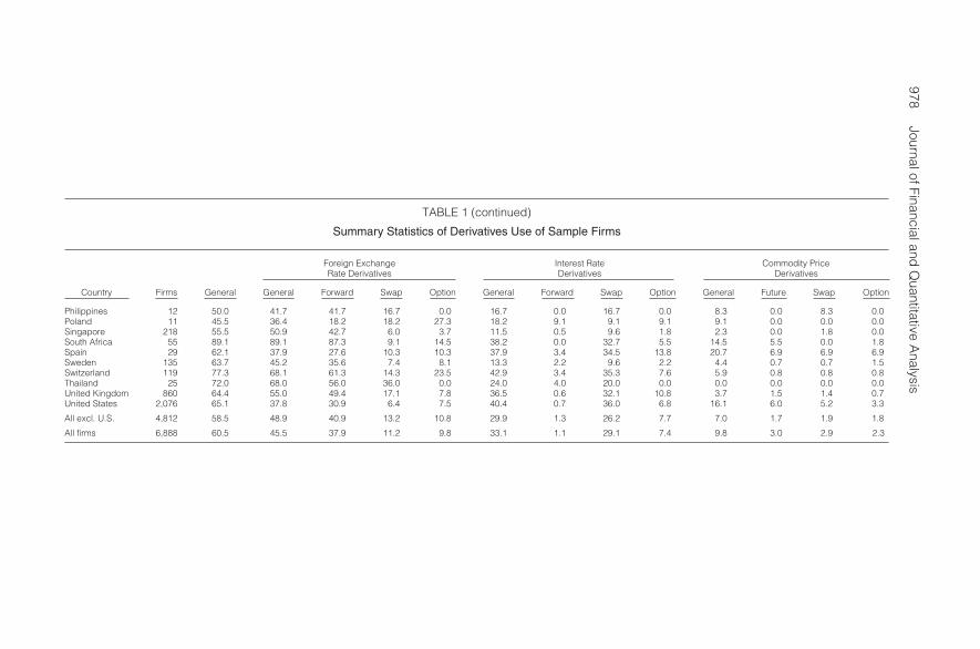
Summary statistics on the use of derivatives by the sample firms is presentedin Table 1. Across all countries, 60.5% of the firms in the sample use at leastone type of derivative. Exchange rate derivatives are the most common (45.5%),followed by interest rate derivatives (33.1%) and commodity price derivatives(9.8%). Though usage rates for particular types of instruments vary consider-ably across countries, some clear patterns emerge. Forward contracts are the mostfrequently used exchange rate derivatives, whereas swaps are the instrument ofchoice for interest rate derivatives. For commodity price derivatives, the distri-bution of instrument type is more even. Firms in the U.S. are less likely to useexchange rate derivatives than non-U.S. firms, but U.S. firms are more frequentusers of interest rate and commodity price derivatives.
All capital market data (i.e., the firms’ stock return indices, stock marketreturn indices, and interest rates) are from Datastream. These data are provided ata daily frequency. For each firm, we calculate stock returns in local currency. Tobegin, all time series are limited to the year of the firm’s annual report. Account-ing data originate from the Thomson Analytics database.14 Outliers are elimi-nated by winsorizing observations in the top and bottom 1 percentile as well asthose observations where variable values exceed more than 5 standard deviationsfrom the median. This filter eliminates some apparent data errors where mag-nitudes suggest data units are not properly reported (e.g., thousands instead ofmillions). Systematic differences across countries and industries are controlledfor with country and 44 industry dummy variables. In order to avoid the cross-sectional results being influenced by the effect of the economic cycle, we use3-year averages of variables where this impact seems most relevant (e.g., cov-erage, foreign income). In a separate analysis, we examine the performance ofderivative users and nonusers through time.
B. Risk Measures
In order to study the possible determinants of corporate derivatives use,different categories of exposures to risk are employed. First, firms may differwith regard to their gross or prehedging exposure.15 For instance, measures ofgross exposure with regard to foreign exchange rate risk include foreign sales(relative to total sales), foreign income (relative to total income), and foreignassets (relative to total assets). In addition to these individual proxies of foreign
13Dichotomous variables for the use of foreign debt and stock options are created in the samefashion, since this information is not readily available elsewhere.
14Data are commonly reported in millions of U.S. dollars. Many of the variables we examine areratios and are therefore largely comparable across countries and years. However, we also examine adummy variable for the year (2000 or 2001) and have undertaken robustness checks to make sure thatour conclusions are not driven by which year we examine.
15To be precise, gross (or prehedging) exposure is a measure of exposure that does not incorporatethe effect of financial derivatives.

Bartram
,Brow
n,andC
onrad977
TABLE 1
Summary Statistics of Derivatives Use of Sample Firms
Table 1 presents summary statistics of derivatives use by country. In particular, it presents the number of firms and the percentage of firms using derivatives, for general derivatives use, foreign exchange ratederivatives, interest rate derivatives, and commodity price derivatives. Firms are required to be outside the financial and regulated utility sectors, and to have an annual report on the Global Reports database,accounting data on Thomson Analytics, and at least 36 nonmissing daily stock returns for the year of the annual report on Datastream. We create a category called “Other countries” for countries with less than10 observations (i.e., Bahamas, Bermuda, Cayman Islands, Egypt, Indonesia, Peru, Portugal, Turkey, and Venezuela).
Foreign Exchange Interest Rate Commodity PriceRate Derivatives Derivatives Derivatives
Country Firms General General Forward Swap Option General Forward Swap Option General Future Swap Option
Argentina 10 70.0 70.0 40.0 20.0 0.0 60.0 0.0 40.0 30.0 40.0 0.0 20.0 30.0Australia 301 66.4 52.2 48.5 8.6 17.9 42.2 3.7 38.9 15.0 14.3 2.0 3.7 5.0Austria 41 56.1 56.1 43.9 17.1 22.0 22.0 0.0 17.1 7.3 7.3 2.4 4.9 2.4Belgium 60 50.0 36.7 26.7 8.3 6.7 23.3 0.0 21.7 3.3 3.3 0.0 1.7 0.0Brazil 16 81.3 56.3 18.8 25.0 12.5 18.8 0.0 12.5 6.3 18.8 0.0 6.3 0.0Canada 537 60.3 46.2 34.3 8.0 8.2 27.2 0.4 24.2 3.2 17.7 2.8 5.2 5.4Chile 13 100.0 84.6 61.5 23.1 7.7 53.8 0.0 38.5 7.7 15.4 0.0 7.7 7.7China 32 12.5 6.3 6.3 3.1 0.0 3.1 0.0 3.1 0.0 3.1 3.1 0.0 0.0Czech Republic 23 26.1 13.0 13.0 4.3 4.3 17.4 0.0 13.0 0.0 0.0 0.0 0.0 0.0Denmark 80 87.5 80.0 72.5 12.5 18.8 26.3 1.3 21.3 6.3 5.0 1.3 2.5 1.3Finland 100 64.0 58.0 45.0 18.0 27.0 37.0 9.0 29.0 17.0 8.0 3.0 1.0 3.0France 159 66.0 52.8 37.1 22.6 25.8 44.7 1.9 38.4 15.1 3.8 1.3 1.3 0.6Germany 395 47.1 39.0 27.3 10.6 12.4 24.1 1.8 17.7 9.4 4.8 1.8 0.5 0.5Greece 19 21.1 21.1 10.5 5.3 5.3 10.5 0.0 10.5 0.0 5.3 5.3 0.0 0.0Hong Kong 319 23.2 18.5 13.8 4.4 1.3 7.2 0.3 5.6 1.3 0.3 0.0 0.0 0.0Hungary 15 40.0 33.3 33.3 6.7 13.3 13.3 0.0 13.3 0.0 13.3 0.0 6.7 0.0India 40 70.0 62.5 60.0 7.5 0.0 12.5 0.0 12.5 0.0 5.0 2.5 0.0 0.0Ireland 46 84.8 69.6 63.0 28.3 8.7 52.2 4.3 47.8 8.7 13.0 2.2 6.5 4.3Israel 48 72.9 68.8 43.8 2.1 22.9 12.5 0.0 10.4 4.2 2.1 2.1 0.0 0.0Italy 93 61.3 38.7 29.0 16.1 3.2 33.3 3.2 23.7 3.2 2.2 1.1 2.2 0.0Japan 366 81.1 75.4 71.0 33.1 17.8 60.4 0.5 59.3 14.2 9.6 3.8 1.6 1.6Korea, Republic of 24 70.8 54.2 41.7 20.8 12.5 25.0 0.0 25.0 0.0 8.3 0.0 0.0 4.2Luxembourg 11 63.6 45.5 45.5 9.1 18.2 27.3 0.0 18.2 9.1 9.1 9.1 0.0 0.0Malaysia 289 20.1 16.3 12.5 1.4 0.7 4.2 0.0 3.8 1.0 1.0 0.7 0.0 0.0Mexico 35 60.0 34.3 25.7 5.7 11.4 37.1 2.9 37.1 0.0 14.3 8.6 2.9 2.9Netherlands 131 56.5 48.1 38.9 18.3 12.2 33.6 1.5 27.5 9.2 4.6 0.8 0.8 0.8New Zealand 39 94.9 79.5 74.4 17.9 35.9 76.9 5.1 71.8 33.3 17.9 0.0 10.3 10.3Norway 85 67.1 56.5 48.2 17.6 17.6 29.4 2.4 24.7 5.9 8.2 2.4 0.0 3.5Other countries 21 52.4 42.9 33.3 19.0 4.8 9.5 0.0 9.5 0.0 9.5 0.0 4.8 9.5
(continued on next page)
978JournalofFinancialand
Quantitative
Analysis
TABLE 1 (continued)
Summary Statistics of Derivatives Use of Sample Firms
Foreign Exchange Interest Rate Commodity PriceRate Derivatives Derivatives Derivatives
Country Firms General General Forward Swap Option General Forward Swap Option General Future Swap Option
Philippines 12 50.0 41.7 41.7 16.7 0.0 16.7 0.0 16.7 0.0 8.3 0.0 8.3 0.0Poland 11 45.5 36.4 18.2 18.2 27.3 18.2 9.1 9.1 9.1 9.1 0.0 0.0 0.0Singapore 218 55.5 50.9 42.7 6.0 3.7 11.5 0.5 9.6 1.8 2.3 0.0 1.8 0.0South Africa 55 89.1 89.1 87.3 9.1 14.5 38.2 0.0 32.7 5.5 14.5 5.5 0.0 1.8Spain 29 62.1 37.9 27.6 10.3 10.3 37.9 3.4 34.5 13.8 20.7 6.9 6.9 6.9Sweden 135 63.7 45.2 35.6 7.4 8.1 13.3 2.2 9.6 2.2 4.4 0.7 0.7 1.5Switzerland 119 77.3 68.1 61.3 14.3 23.5 42.9 3.4 35.3 7.6 5.9 0.8 0.8 0.8Thailand 25 72.0 68.0 56.0 36.0 0.0 24.0 4.0 20.0 0.0 0.0 0.0 0.0 0.0United Kingdom 860 64.4 55.0 49.4 17.1 7.8 36.5 0.6 32.1 10.8 3.7 1.5 1.4 0.7United States 2,076 65.1 37.8 30.9 6.4 7.5 40.4 0.7 36.0 6.8 16.1 6.0 5.2 3.3
All excl. U.S. 4,812 58.5 48.9 40.9 13.2 10.8 29.9 1.3 26.2 7.7 7.0 1.7 1.9 1.8
All firms 6,888 60.5 45.5 37.9 11.2 9.8 33.1 1.1 29.1 7.4 9.8 3.0 2.9 2.3

Bartram, Brown, and Conrad 979
exchange rate exposure, we create a variable Gross-FX-Exposure that is equal tothe sum of foreign sales and foreign assets (as percent of totals) multiplied by theratio of home-country exchange rate volatility to average exchange rate volatil-ity (of all countries in our sample). This firm-specific and continuous variableprovides a sensible relative gauge of gross exchange rate exposure, since it in-cludes measures of both the degree of foreign currency operations and the relativevolatility of the domestic currency. Foreign debt may create an exposure as well,but it could also work as a hedge.
Leverage, coverage, or the quick ratio may be indicators for gross interestrate exposure. With regard to commodity price exposure, we define an exposurevariable at the industry level using U.S. input-output data from the Bureau ofEconomic Analysis from calendar year 2000. For each industry in our sample,we sum the value of inputs from commodity-sensitive industries and express it asa percentage of total input values.16 The resulting variable, Gross-CP-Exposure,ranges from a low of 1.6% for the recreation industry to a high of 73.9% forthe oil industry. Finally, firms may also have more incentive to hedge if they areclose to default. We use Altman’s (1968) Z-score measure as a proxy for financialdistress. For any of these measures, if firms are using derivatives primarily forhedging purposes, firms should be more likely to use derivatives if they have highmeasures of exposures.
Next, a firm’s net (or posthedging) exposure is the result of the character-istics of its assets and liabilities, and ideally also includes the effects of off-balance-sheet transactions such as derivatives.17 Our 1st measure of net exposureis operating cash flow volatility (σCF), which we define as the standard deviationof operating margins (operating cash flow divided by total sales) using 5 yearsof annual data. However, operating cash flow may not be a good measure ofnet exposure for several reasons. First, it is not measured with much precisiongiven the limited amount of data. Second, managers may be able to systemati-cally manipulate values for accounting variables. Finally, operating cash flow maynot account for the use of all derivatives for all firms. Specifically, if exchangerate and commodity price derivative transactions do not utilize (i.e., qualify for)“hedge accounting” they will not be reflected in operating cash flow. Similarly,the effects of most interest rate derivatives will not be reflected in operating cashflow.18 However, cash flow volatility will capture other types of risk managementactivities (e.g., operational hedging with foreign assets), which have been identi-fied as important hedging tools for exchange rate risk. Thus, cash flow volatility
16Specifically, we define the following industries as commodity price sensitive: oil and gas ex-traction, mining, utilities, wood products, paper products, petroleum and coal products, chemicalproducts, plastics and rubber products, primary metals, air transportation, water transportation, andtruck transportation.
17To be precise, net (or posthedging) exposure is a measure of exposure that incorporates the effectof financial derivatives.
18Nonetheless, most derivative users in our sample use exchange rate and commodity price deriva-tives. We have also conducted all of our analysis using a measure of earnings, rather than cash flow,volatility; to conserve space, we do not report the results separately. We find similar, albeit slightlyweaker, results for earnings volatility. This may be because firms take on other financial risks (e.g.,greater leverage) if they can hedge some financial risks.

980 Journal of Financial and Quantitative Analysis
may be affected for derivative users, even if derivatives do not qualify for hedgeaccounting, if derivatives are a proxy for broader “corporate hedging.”19
While the risk of assets and liabilities contain different components and theirinteractions are difficult to decompose, the assumption of efficient capital marketssuggests that net exposures can be estimated empirically using a company’s stockprice as an aggregate measure of relevant information. Consequently, we constructdifferent firm-specific risk measures from stock prices. In particular, for each firmwe calculate the standard deviation of its stock returns (σE). We also examinestandardized firm volatility (σ∗E), measured as the ratio of a firm’s stock returnstandard deviation to the standard deviation of the returns of the local marketindex, to avoid a potential bias from a spurious correlation between derivativesuse and overall market volatility.
The sensitivity of the firm’s stock returns to the local market return is esti-mated using the standard market model on daily returns,
Rjt − rft = αj + βj (RMt − rft) + εjt,(1)
where Rjt is the stock return of firm j on day t, RMt is the return on the local marketindex M on day t, and rft is the (daily) risk-free rate of interest.20 The estimationperiod consists of the year for which we have the annual report data. The Newey-West (1987) procedure is used to correct for autocorrelation and heteroskedastic-ity. Corporate use of derivatives for hedging purposes would be consistent withlower stock return volatility and lower measures of posthedging exposures as es-timated in the regression framework. Overall (net) market exposure is measuredby the estimated value βj.
Table 2 reports statistics for the risk variables used in our analysis. Returnsfor individual stocks, pooled across all observations, and the market index arenegative on average over our sample period, –8 basis points (bp) and –4 bp perday, respectively. Average volatility of operating cash flow, σCF, is 8.25% butvery positively skewed. As a result, we also examine the natural logarithm ofoperating cash flow volatility in our statistical analysis. Risk as measured by σE
averages 0.56 and is somewhat positively skewed. Standardizing σE by marketvolatility (σ∗E) suggests that the average firm has substantial idiosyncratic risk,with a standard deviation of return that is more than 2.5 times the market’s volatil-ity. Estimated market betas average 0.70, indicating that the typical firm in oursample has relatively low systematic risk. This is likely due to a selection biasfrom requiring an annual report in English, certain accounting variables, and cap-ital markets data. The resulting firms are typically larger, more global, and moreestablished firms with somewhat lower systematic risk. Despite this, we do seesubstantial cross-sectional dispersion in the beta estimates in the sample (morethan 25% of firms in our sample have estimated values for beta that are greater
19As a robustness check we have repeated all of our tests with other measures of profit volatilityand find similar results to those for cash flow volatility. Specifically, we have examined net margin,ROA, and earnings yield. Selected results using these alternative accounting measures of profits arediscussed in the text.
20As a proxy for the risk-free rate we use 30-day Eurocurrency rates obtained from Datastream or,when these are unavailable, the shortest-term high quality (e.g., government) rate.

Bartram, Brown, and Conrad 981
than 1.0). The betas in our sample are also estimated with a good deal of preci-sion. The median p-value for a 2-tailed test against a null of 0 is 0.001, and morethan 80% of betas are different from 0 at the 10% confidence level.
TABLE 2
Summary Statistics on Capital Market Data and Risk Measures
Table 2 presents the mean, standard deviation (SD), minimum, 5th, 25th, 50th (median), 75th, and 95th percentile aswell as the maximum of selected variables. In particular, it shows capital markets data such as the daily returns of thesample firms and the corresponding returns of the domestic market indices. It also presents descriptive statistics of cashflow volatility (σCF), the annualized SD of local currency stock returns (σE), and the SD of local currency stock returnsstandardized by the SD of the local market index (σ∗E ). Here, β is the coefficient of a regression of stock returns on marketindex returns, and p-value is the corresponding significance level. All variables are defined in Table 3.
Percentiles
Variable Mean SD Min 5th 25th Median 75th 95th Max
Panel A. Capital Markets Data
Stock return –0.08 3.71 –12.52 –6.19 –1.50 0.00 1.24 6.12 13.04Market return –0.04 1.44 –18.24 –2.31 –0.79 0.00 0.73 2.23 17.03
Panel B. Risk and Value Measures
σCF (%) 8.25 12.65 0.59 0.59 1.59 3.36 7.91 50.83 52.91σCF (log) 1.34 1.19 –0.52 –0.52 0.46 1.21 2.07 3.93 3.97σE 0.56 0.23 0.18 0.25 0.37 0.51 0.71 1.01 1.16σ∗E 2.56 1.14 0.72 1.10 1.70 2.32 3.24 4.74 6.05β 0.70 0.58 –0.18 0.01 0.27 0.57 1.01 1.89 2.55β (p-values) 0.10 0.21 0.00 0.00 0.00 0.00 0.07 0.65 1.00q 2.33 2.67 0.42 0.62 1.00 1.43 2.48 7.18 21.22q (log) 0.51 0.74 –0.86 –0.48 0.00 0.36 0.91 1.97 3.06
We define a proxy for Tobin’s q (q) as the sum of equity market capitaliza-tion, the book value of total debt, and the book value of preferred stock dividedby the book values of each of these financing sources. The average q in our sam-ple is 2.33. The primary advantage of this method is its simplicity, which allowsus to create values for nearly all firms in our sample. Alternative measures, suchas those used by Allayannis and Weston (2001), rely on the use of segment andindustrywide investment data that are not available for many of the firms in ourglobal sample. Table 2 also shows that q is very positively skewed. This skewnessis consistent with the results of many other researchers. As a consequence, simi-lar to Allayannis and Weston, we also examine the natural logarithm of q in ourstatistical analysis.21
IV. Methodology
A. Propensity Score Matching
Previous results in the literature, which we confirm in our sample, sug-gest that there are substantive differences, on average, in the characteristics offirms that use derivatives and those that do not. These differences generate a se-lection bias when estimating the effect of derivatives on a firm and should be
21In the subsequent analysis, we only tabulate results using the natural logarithms of σCF and q forbrevity. However, we have also conducted all of our analysis using the levels of σCF and q. The resultsusing those levels are qualitatively similar and usually statistically stronger.

982 Journal of Financial and Quantitative Analysis
controlled for when we estimate the effect that derivatives have on risk and marketvalues. Ideally, one would like to estimate the “treatment” effect by observingthe same firm, under identical economic conditions, with derivatives and withoutderivatives in place. Since this is not possible, the 1st method we use attempts toconstruct a “similar” firm to the user, where to the extent possible the “similar”firm differs only in its choice not to use derivatives.
TABLE 3
Variable Definitions
Table 3 reports the variables of the study and their definitions.
Variable Definition
Derivatives Dummy variables with value 1 if firm uses derivatives, and 0 otherwise.Foreign assets International assets / total assets.Foreign income International operating income / operating income (3-year average).Foreign sales International sales / net sales or revenues (missing set to 0).Gross-FX-Exposure Sum of foreign sales and foreign assets (as percent of totals) multiplied by the ratio of home-
country exchange rate volatility to average exchange rate volatility (of all countries inour sample).
Foreign debt Dummy variable with value 1 if any foreign debt is reported, and 0 otherwise.Leverage Total debt / size.Coverage Earnings before interest and taxes (EBIT) / interest expense on debt (3y).Quick ratio (Cash & equivalents + receivables (net)) / total current liabilities.Z-score Altman’s Z-score (6.56× (working capital / total assets) + 3.26× (retained earnings / total
assets) + 6.72× (EBIT / total assets) + 1.05× (book value of equity + preferred stock) /total debt).
Gross-CP-Exposure Defined at the industry level using U.S. input-output data from the Bureau of EconomicAnalysis from calendar year 2000. For each industry, we sum the value of inputs fromcommodity-sensitive industries, and express it as a percent of total input values.
Industry segments Number of business segments (Standard Industrial Classification (SIC) codes) that makeup the company’s revenue (between 1 and 8).
Size (log) Natural logarithm of the sum of market capitalization, total debt, and preferred stock.Sales (log) Natural logarithm of total sales.Dividend (dummy) Dummy variable with value 1 if dividend yield, dividend payout, or dividend per share is
positive, and 0 otherwise.Gross profit margin Gross income / net sales or revenues (3-year average).Book-to-market Book value per share / market price-year end.ROA Return on assets (3-year average).Cash flow Operating income / sales.R&D / sales Research and development expense / sales (missing set to 0).Earnings yield Earnings per share / end-of-year share price of common stock.CAPEX / sales Capital expenditures / net sales or revenues (missing set to 0).Tangible assets (Total assets – intangibles) / total assets.Tobin’s q (log) Size / (book value of equity + total debt + preferred stock) (natural logarithm).Multiple share class Dummy variable with value 1 if currently multiple share classes exist, and 0 otherwise.Stock options Dummy variable with value 1 if stock options are reported in the annual report, and 0
otherwise.Stock return Daily stock return in local currency.Market return Daily local stock market return in local currency.Cash flow volatility (σCF) 5-year standard deviation of operating cash flow / sales.σE Standard deviation of local currency stock returns (annualized).σ∗E Ratio of the daily local currency stock return standard deviation and the local currency
market index standard deviation.β Coefficient of the market index from a regression of local currency stock returns on returns
of the local market index.β (p-value) p-value of the coefficient of the market index from a regression of local currency stock
returns on returns of the local market index.Alpha Intercept from a regression of local currency stock returns on returns of the local market
index.Sales growth 4-year growth rate of sales (4y).Age (log) Natural logarithm of the age of the firm in years.Derivative market rank Inverse ranking of the size of the derivatives market relative to the market of the other coun-
tries in the sample. Size is calculated by summing daily turnover in the exchange rateand interest rate markets in 2001 for nonfinancial firms and standardizing by nominalGDP. We use the rank because the unranked values are extremely positively skewedby countries with exchange rate trading centers (e.g., the U.K.).
Rather than matching on several individual firm characteristics or covariates,the method we choose matches on the propensity score (the estimated likelihood
Bartram, Brown, and Conrad 983
that a firm will use derivatives). Rosenbaum and Rubin (1983) show that matchingon the covariates and matching on the propensity score will both result in a dis-tribution of the covariates in the treated and untreated groups that is the same. Anadvantage of propensity score matching is that it eliminates the “curse of dimen-sionality” when one wishes to match on several characteristics. A disadvantageof propensity score matching is that a large sample is required to obtain a mean-ingful match on the propensity scores (i.e., one that allows for a precise mea-surement of the treatment effect). (See Zhao (2004) for more discussion on thispoint.)
To use this method, we model the likelihood that a firm will choose to usederivatives, H(Wi), based on a set of variables Wi. That is, we model
Hi = γ′Wi + ui,(2)
where the observed value of Hi is 1 if the firm chooses to use derivatives, and 0otherwise. The variables Wi are the characteristics of the firm that are expected toinfluence the choice of whether a firm uses derivatives. After the propensity scoresare estimated, one can choose to match a user to the single nonuser with the mostsimilar propensity score, or to a weighted grouping of nonusers, whose weighted-average propensity score is similar to that of the user. One can match with or with-out replacement and also set up boundaries or “calipers” of various magnitudes,outside of which no matches are chosen. We use various combinations of thesechoices to ensure that our results are robust. We also examine various choices ofthe variables that are presumed to influence derivative use, Wi.
B. Selection Bias
Clearly, if there are unobserved or hidden variables that affect the decisionto use derivatives, a bias may remain in the estimated effect. One advantage ofthe propensity score matching technique is that it allows for a sensitivity analysison this selection bias. Rosenbaum (2002) shows that it is possible to construct anupper bound on the influence that any omitted variable would have to have onthe hedging choice in order to overturn the inferences drawn. We estimate thisbound and provide a comparison to the effect that any hidden bias must have,relative to the influence of the observable characteristics of the firms, to overturnthe original inference. Thus, while we are not able to rule out the influence of ahidden characteristic, we can provide a benchmark for how large the effect wouldhave to be, compared to well-known firm characteristics, to change the inferencesdrawn from the analysis.
C. Variable Choice
Many firm characteristics have been hypothesized to be relevant for therelationship between derivatives use and measures of risk and value and are there-fore candidates for use as control variables. In particular, derivative use has beenshown to be related to industrial diversification (number of industry segments),firm size (natural logarithm of total assets or alternatively the sum of equitymarket capitalization, total debt, and preferred stock), and tangible assets (as a

984 Journal of Financial and Quantitative Analysis
fraction of total assets). Firms with more growth options, as measured by researchand development (R&D) expenses (relative to total sales) and capital expenditures(CAPEX) (relative to total sales) have been shown to be more likely to use deriva-tives (see, e.g., Geczy et al. (1997)). As Jin and Jorion (2006) point out, firms incertain industries may be more likely to hedge if, for example, they are exposedto more readily identified, larger, or more easily hedged types of risk.
Finally, access to derivatives markets could have an important effect on afirm’s ability to execute hedging strategies. Alternatively, easy access to deriva-tives may facilitate engaging in derivatives transactions for purposes other thanhedging because the costs of entering transactions (or more generally markets)are lower and therefore less likely to require extraordinary actions on the part ofmanagers. As a proxy for access to derivatives markets, we use a proxy for the rel-ative size of the derivatives market in a company’s home country as measured bythe derivatives market rank (Bartram, Brown, and Fehle (2009)). The definitionsof these variables as well as others subsequently used in the analysis are presentedin Table 3.
V. Results
A. Univariate Results
To begin, we compare the simple averages of risk characteristics in oursample categorized by derivative use. These results are presented in Table 4.We measure the significance of differences between the 2 types of firms usingnonparametric Wilcoxon tests. Table 4 reports the p-values of these tests togetherwith the means, medians, and differences in means of firm characteristics forderivative users and nonusers. While the results in Table 4 only refer to gen-eral derivatives use, the tests are also conducted separately for foreign exchangerate derivatives, interest rate derivatives, and commodity price derivatives, anddifferences are mentioned in the text where appropriate.
Panel A of Table 4 shows that firms using derivatives are more exposed to ex-change rate risk on a prehedging basis: They have significantly more foreign sales,foreign income, foreign assets, and higher Gross-FX-Exposure. This is consistentwith the use of derivatives for hedging. As measured by the existence of for-eign debt, the liabilities of derivative users are also significantly more exposed toexchange rate risk (though foreign debt is also used as a risk management tool bymany multinational corporations). In addition, derivative users have significantlyhigher gross interest rate exposure, as measured by higher leverage and lowerquick ratios. In contrast, users have higher coverage ratios. Firms are more likelyto belong to commodity-sensitive industries if they use derivatives (we observe ahigher mean Gross-CP-Exposure for firms that use derivatives compared to thosethat do not). Overall, the results strongly suggest that firms are more likely touse derivatives if they have higher gross (i.e., prehedging) exposure. These tests,based on firm characteristics, are robust to analyzing derivatives separately onexchange rate risk, interest rate risk, or commodity price risk.
For most firms, asset and liability risks are unlikely to be independent. Con-sequently, we examine more comprehensive risk measures based on the firms’

Bartram, Brown, and Conrad 985
TABLE 4
Univariate Tests of Corporate Risk Measures and Derivatives Use
Table 4 presents the number of observations (N), mean, median, and difference in mean of different risk characteristics forderivative users and derivative nonusers. The last column presents p-values of Wilcoxon rank sum tests between derivativeusers and nonusers. All variables are defined in Table 3.
User NonuserDifference Wilcoxon
Variable N Mean Median N Mean Median in Means p-Value
Panel A. Gross Exposure
Foreign sales 4,167 0.272 0.152 2,721 0.164 0.000 0.108 <0.001Foreign income 2,421 0.235 0.056 1,477 0.143 0.000 0.092 <0.001Foreign assets 2,349 0.182 0.099 1,205 0.114 0.000 0.068 <0.001Gross-FX-Exposure 4,167 0.379 0.196 2,721 0.176 0.000 0.203 <0.001Foreign debt 4,167 0.882 1.000 2,721 0.725 1.000 0.157 <0.001Leverage 4,091 0.297 0.254 2,643 0.189 0.081 0.108 <0.001Quick ratio 4,052 1.380 0.913 2,616 2.455 1.345 1.075 <0.001Coverage 4,114 3.852 3.657 2,655 2.542 3.333 1.310 <0.001Gross-CP-Exposure 4,167 0.151 0.106 2,721 0.114 0.051 0.100 <0.001
Panel B. Net Risk and Value
σCF (%) 3,365 6.200 2.848 1,768 12.162 4.994 –5.962 <0.001σCF (log) 3,365 1.144 1.046 1,768 1.717 1.608 –0.573 <0.001σE 4,167 0.510 0.461 2,721 0.624 0.604 –0.114 <0.001σ∗E 4,167 2.380 2.140 2,721 2.842 2.705 –0.462 <0.001β 4,165 0.686 0.540 2,721 0.732 0.618 –0.046 <0.001q 3,980 2.154 1.392 2,559 2.605 1.564 –0.451 0.005q (log) 3,980 0.480 0.331 2,559 0.556 0.447 –0.076 0.005Alpha 4,165 –0.061 0.008 2,721 –0.236 –0.114 0.175 <0.001
Panel C. Other Firm Characteristics
Z-score 3,566 5.515 3.471 1,971 8.888 5.688 –3.373 <0.001Size (log) 4,126 6.580 6.555 2,680 4.783 4.731 1.797 <0.001Sales (log) 4,091 6.713 6.691 2,643 5.063 4.941 1.650 <0.001Industry segments 4,150 3.823 3.000 2,710 3.420 3.000 0.403 <0.001Dividend (dummy) 4,167 0.598 1.000 2,721 0.400 0.000 0.198 <0.001R&D / size 4,167 0.044 0.000 2,721 0.121 0.000 –0.077 <0.001CAPEX / size 4,172 0.126 0.050 2,724 0.174 0.047 –0.048 0.011Tangible assets 3,882 0.874 0.943 2,554 0.888 0.973 –0.014 <0.001Stock options 4,172 0.828 1.000 2,724 0.792 1.000 0.036 <0.001Sales growth 3,452 10.513 6.450 1,821 13.774 8.861 –3.261 <0.001Derivative market rank 4,167 38.299 43.000 2,721 36.083 41.000 2.216 <0.001
cash flow measures and stock returns. Studying stock prices is informative, sincethey represent an aggregate measure of asset and liability risk and should alsoincorporate the effects of financial risk management. If derivatives are used forhedging purposes, firms with high prehedging exposure should be more likely touse them and, consequently, might exhibit similar, or even lower, posthedging(net) exposure.
Despite the higher exposures documented in Panel A of Table 4, the univari-ate results in Panel B of Table 4 shows that derivative users have significantlylower cash flow volatility, total risk, and market risk. In particular, the averageσCF (log) is more than 30% lower for users, and σE and σ∗E are about 20% lowerfor derivative users. Likewise, market betas are on average about 6% lower forderivative users. These results provide some support for the hypothesis that, onaverage, firms are hedging rather than speculating with derivatives. At a univari-ate level, the unadjusted Tobin’s q of the average derivative user is 17% lowerthan for the average firm that does not use derivatives. However, we also see thatthe unconditional relative performance of users as measured by the market-modelalpha is significantly higher in our sample period.
986 Journal of Financial and Quantitative Analysis
Panel C of Table 4 shows that there are further significant differences in thecharacteristics of firms that use derivatives and those that do not. For example,derivative users have lower Z-scores, are significantly larger, and are more diver-sified. They are also more likely to pay dividends and to have executive stockoptions. However, derivative users also tend to have fewer tangible assets, lowerR&D expenses, and lower CAPEX. As expected, firms are more likely to usederivatives if the market for derivatives (among dealers) is more developed.
We repeat the analysis for the firm-specific variables in Table 4 after eachvariable has been adjusted for country and industry fixed effects (results are nottabulated). The results are largely unaffected, although in some instances statisti-cal significance is reduced. The most striking difference in this respect is that usersno longer have a significantly lower q after taking country and industry effectsinto account. The results for risk measures are quite similar to those presented inTable 4. Overall, the univariate results suggest that nonfinancial firms use deriva-tives in line with hedging motives. These findings also clearly show large dif-ferences in the characteristics of derivative users and nonusers that should becontrolled for. In the next section, we undertake a multivariate analysis for thispurpose.
B. Multivariate Results
1. Propensity Score Matching: Risk Measures
We begin with a matching analysis. Specifically, we match derivative userswith nonusers on the basis of their propensity score, which is a measure of thefirms’ propensity to use derivatives based on the firms’ unique characteristics.Several choices must be made in order to use propensity score matching. As inany matching analysis, in making these choices we are trading off the precisionof the matching criteria against the sample size. We explore a number of differentspecifications and present several representative specifications. In general, ourresults are robust across most specifications; we note differences in results wherethey occur.
In conducting the propensity score matching the first choice is the selectionof independent variables that are hypothesized to influence firms’ likelihood ofusing derivatives. We use variables that have been shown elsewhere to be associ-ated with derivative use and risk exposure, as well as variables that incorporate thebroader nature of our sample. Specifically, we include Altman’s (1968) Z-score,firm size, leverage, a liquidity variable (quick ratio), and a market access variable(a dummy variable for multiple share classes). In some specifications we alsoinclude a variable related to managerial incentives to hedge (stock option use),Gross-FX-Exposure, a dummy variable for existence of foreign currency debt, aswell as country and industry dummy variables (where noted). For q, we also in-clude variables shown by other studies to be associated with firm value such asdividend payout, sales growth, R&D expenditures, and CAPEX.
The most important determinants of derivatives use are not surprising.Consistent with the univariate results, firm size, leverage, the multiple share classdummy variable, the stock options dummy variable, exchange rate exposure,and the foreign debt dummy variable are positively related to the probability

Bartram, Brown, and Conrad 987
of derivative use, whereas the Z-score and quick ratio exhibit negative relations.In addition, many, but not all, industry and country dummy variables are statisti-cally different from each other. Furthermore, matching on these factors is impor-tant for our analysis, since other studies have shown some to be related to risk andvalue measures. For example, Bartram, Brown, and Stulz (2011) find that firmsize, leverage, and liquidity are important determinants of both total risk and sys-tematic risk. Allayannis and Weston (2001) find that size, growth, leverage, anddividends are related to firm value. The relations we observe are intuitive (resultsare not tabulated). Larger firms are likely to have more stable sales and thus lowercash flow and equity price risk. Conversely, firms with more financial leverage orthat have a higher chance of financial distress should have higher risk. Firm valueis increasing in firm profitability and growth, since these lead to higher cash flowsto equity holders, but is decreasing with age and size, since these firms are likelyto be more established and thus less likely to have large new profit opportunities.
The second choice in the matching analysis is the construction of the match-ing nonuser. The analysis can simply choose a single, “nearest neighbor” match,or use a weighted average of many (or all) nonusers to construct a match. One cansample from the nonusers with or without replacement. One can set conditionsoutside of which no matches will be found (i.e., caliper matching). We conductour analysis using 2 different matching criteria (with and without replacement),and 3 different choices of matching parameters, for 6 specifications in all.
In assessing the propensity score method’s success, it is important to knowthe extent to which the propensity score matching succeeds in removing theselection bias in the observed characteristics of firms in the 2 subsamples. Conse-quently, for each characteristic, we calculate the bias measure
BIAS =
∣∣∣∣∣∣100(μT − μC)√(s2
T + s2C)/2
∣∣∣∣∣∣,(3)
where μT and sT are the sample mean and standard deviation of the character-istic for the user, and μC and sC are the sample mean and standard deviationfor the characteristic in the matching control firms, respectively. In general, thematching methods substantially reduce the difference in characteristics across testand matched firms (although to save space, we do not tabulate the results). With-out propensity score matching, we find that the bias in the characteristics in theraw data is quite large; for example, the bias in market capitalization is greaterthan 90%, while the biases in leverage, foreign exposure, and foreign debt areall greater than 40%. The specifications that allow for replacement of the non-treated firms in the sample reduce the bias so that none of the characteristics isassociated with a bias of more than 16%, and most are below 10%.22 Overall, thematching procedure does a good job of producing “balanced covariates” acrossthe 2 subsamples.
22While both of the matching specifications we consider reduce the bias considerably, the spec-ification that does not allow for replacement still contains substantial biases with respect to marketcapitalization, foreign debt, and foreign exchange rate exposure.

988 Journal of Financial and Quantitative Analysis
In the subsequent analysis, we examine results from all 6 methods but onlyreport results using matching with replacement to save space. We discussdifferences when appropriate. We prefer the results with replacement because thisleads to greater reductions in selection bias (as noted previously), maximizes thesample size of derivative users, and eliminates the need to determine which deriva-tive users to include in the analysis. Regardless, our conclusions are not sensitiveto whether we examine results of tests with or without replacement.
Table 5 presents the results of representative propensity score estimation foreach of the 4 primary variables we examine (σCF, σE, β, and q). For each ofthese 4 variables, we report the number of firms, mean, and median values of thecharacteristic for the firms that use derivatives and those that do not, and providea measure of the difference in means as well as a statistical test of the significanceof the difference between the 2 subsamples of firms.
TABLE 5
Matched-Sample Tests of Corporate Risk Measures and Derivatives Use
Table 5 presents the number of observations (N), mean, and median of different outcome variables for derivative usersand derivative nonusers. The last column presents p-values of Wilcoxon rank sum tests between derivative users andnonusers. Results are tabled for cash flow volatility (σCF), total risk as measured by the annualized standard deviation ofstock returns (σE), market betas (β) estimated using equation (1), and Tobin’s q. Specification 1 reports results for cashflow volatility, stock return volatility, and market betas using the independent variables: Z-score, leverage, quick ratio,size (log), multiple share classes, stock options, gross exchange rate exposure, foreign currency debt, and industry andcountry dummy variables, and for Tobin’s q, the independent variables Z-score, sales growth, R&D / size, CAPEX / size,age (log), quick ratio, sales (log), dividend (dummy), multiple share classes, stock options, gross exchange rate exposure,foreign currency debt, and industry and country dummy variables. Specification 2 reports results for the same variables asspecification 1 except gross exchange rate exposure, foreign currency debt but also uses the matching options “caliper(0.01) trim(1) common.” Specification 3 reports results for cash flow volatility, stock return volatility, and market betasusing the independent variables: Z-score, size (log), leverage, multiple share classes, quick ratio, and for Tobin’s q, theindependent variables Z-score, sales growth, R&D / size, CAPEX / size, age (log), sales (log), dividend, and multiple shareclasses. All variables are defined in Table 3.
Users Nonusers
Variable: Country and Diff. in WilcoxonSpecification Industry Dummies N Mean Median Mean Median Means p-Value
σCF (log):1 Yes 2,440 0.997 0.907 1.074 0.945 –0.077 <0.0012 Yes 2,440 0.996 0.907 1.152 1.019 –0.156 <0.0013 No 2,510 1.000 0.913 1.215 1.110 –0.215 <0.001
σE:1 Yes 3,490 0.500 0.456 0.524 0.495 –0.024 <0.0012 Yes 3,490 0.500 0.456 0.546 0.512 –0.046 <0.0013 No 3,507 0.498 0.454 0.551 0.519 –0.053 <0.001
β:1 Yes 3,490 0.663 0.528 0.745 0.653 –0.138 <0.0012 Yes 3,490 0.663 0.528 0.757 0.700 –0.113 <0.0013 No 3,507 0.661 0.528 0.806 0.712 –0.249 <0.001
q:1 Yes 2,076 0.451 0.312 0.385 0.255 0.066 0.0152 Yes 1,956 0.453 0.323 0.401 0.291 0.052 0.0893 No 2,137 0.454 0.315 0.329 0.238 0.125 <0.001
Regardless of the parameters chosen for the construction of the matchingnonderivative users, we find significantly lower values for cash flow volatility(σCF), standard deviation of returns (σE), and beta risk (β) for firms that usederivatives. Across the various specifications, the differentials in σCF range fromapproximately 8% to 20%; for σE the reduction varies from between 5% to 10%;the differential in β varies from between 15% and 31%. Calculating the differ-entials using medians gives a similar result, as do all the other specifications we

Bartram, Brown, and Conrad 989
consider. Differences of this magnitude should have a material effect on a firm’scost of capital. For example, consider the capital asset pricing model (CAPM)with a 5% market risk premium; a decline in β of 0.15 results in a 75-bpreduction in the cost of equity.
Regardless of the specification, we find that the average values of q for firmsthat use derivatives are higher than for those that do not; however, the result isstatistically weaker than the risk results, with p-values across specifications rang-ing between <0.001 and 0.100. The magnitude of the estimated effect also variesacross different specifications, but is always economically large, ranging fromabout 7% to 14% (in levels).
The results in Table 5 suggest that, after controlling for other firm char-acteristics, derivative contract use is associated with statistically and econom-ically significantly lower cash flow and stock return volatility, as well as withlower systematic risk. The statistical evidence for an increase in value is weaker;however, the economic magnitude of the estimated change in value is alwaysnontrivial.
2. What about the Selection Bias?
Although the propensity score matching represents one way to correct forselection bias, it assumes that all of the differences between firms that drive thedifference in derivative use are observable; Rosenbaum and Rubin (1983) callthis assumption “unconfoundedness.” More specifically, they assume that obser-vations with the same propensity score have the same distribution of unobservablecharacteristics, independent of their treatment status. If this assumption does nothold then there will be a hidden bias in the results. That is, if there are unobservedvariables that affect whether a firm decides to use derivatives, as well as the riskand value outcomes, then our inferences may be incorrect.
Since the problem variables are, by definition, unobserved, we cannotestimate their effect directly. However, using the propensity score matching tech-nique, Rosenbaum (2002) calculates a bound on how large an effect the unob-served variables would have to have on the selection process in order to changethe inferences provided by the propensity score matching analysis. Intuitively,this bound is based on the calculation of an odds ratio. If 2 firms have identi-cal observable characteristics, the expected value of the odds ratio that they willchoose to use derivatives is 1 in the absence of a hidden bias. However, if there isa hidden bias in the estimation, and the firms differ in the unobserved character-istic, then the chance that the firms will differ in their choice of derivatives variesmore widely, and the precision of the inferences declines. The calculation of thebounds is essentially a sensitivity analysis; first, one sets the size of the hiddenbias, and thus the size of its effect on the odds ratio, to a particular level. Next,following Rosenbaum, one recalculates a new (larger) confidence interval for thep-value on the difference of each of the relevant characteristics based on this levelof hidden bias. The level of hidden bias is then incremented, and the recalculationis repeated.23 As DiPrete and Gangl (2004) point out, the Rosenbaum bound is
23We calculate these bounds individually for each characteristic. Although one could in theorycalculate a joint bound for a combination of variables, this requires that one assumes, or separately

990 Journal of Financial and Quantitative Analysis
a “worst-case” scenario: It tells the observer not that the treatment effect is notpresent, but at what point the confidence interval would include 0 “if this [unob-served] variable’s effect . . . was so strong as to almost perfectly determine [theeffect of derivative use] for each pair of matched cases in the data.” In that respect,the results of the Rosenbaum bound analysis are conservative.
In Table 6, we calculate the Rosenbaum (2002) bounds for the matchingspecifications presented in Table 5, where the variables of interest are σCF, σE, β,and q. The gamma variable indicates the generated, or preset, size of the hiddenbias for each specification, which is required for the critical p-value associatedwith that inference to be larger than 0.05. For example, a gamma of 1.5 indicatesthat the unobserved variable is associated with a 50% change in the odds ratioof whether a firm uses derivatives. In row 1 of Panel A, the bias level (gammavalue) of 1.18 is associated with the critical probability of 5%; thus, to overturnthe inference on cash flow volatility in the data, or, equivalently, to become lessthan 95% confident that derivative use is associated with a decline in cash flowvolatility, users would have to be 18% more likely to possess some hidden traitthan nonusers. Clearly, higher values of gamma suggest a less important potentialhidden bias problem.
Once the bound is calculated, the interpretation of how severe the hiddenbias problem is, or the economic interpretation of the level of gamma required tooverturn inferences, is subjective. However, following DiPrete and Gangl (2004),we can compare the change in inferences, which is potentially caused by unob-served variables, given by the Rosenbaum (2002) bounds, to the equivalent effectof observed variables, since we have estimates of the effect of the observables onthe decision to use derivatives. These values are given in the remaining (numeric)columns of Table 6.
For example, in the first specification for σE, we see that for an unobservedvariable to cause a hidden bias that affects our inferences on standard deviationof total return, that variable would have to have an effect equivalent to at least adifference of 0.40 in leverage. This difference is approximately twice the averageleverage level of nonusers in the sample, or approximately 1.5 times the standarddeviation of leverage for nonusers. Similarly, a missing variable would have tobe equivalent to the effect of a difference in log size of 1.07. This represents adollar difference of about $2 billion, or several times the average market value ofnonusers in our sample.
The general interpretation for the inferences on the effect of derivative use ontotal risk and systematic risk is similar: To overturn the inference that derivativeuse reduces risk, an unobserved confounding variable must have an impact thatis comparable in magnitude to economically large changes in firm characteristics,such as leverage, market capitalization, or risk exposure. Moreover, such an un-observed variable would have to be unrelated to the other control variables weuse. The inferences for the effect of derivative use on cash flow risk appear to be
estimates, the relation between the combination of characteristics of interest (see DiPrete and Gangl(2004) for an example of such a specification). Given the large number of characteristics we consider,and the difficulty in estimating their interrelationships, we do not perform such an analysis. Conse-quently, the bounds we report should be interpreted with some caution. It is certainly possible thatsmaller changes in multiple variables would be sufficient to overturn inferences.
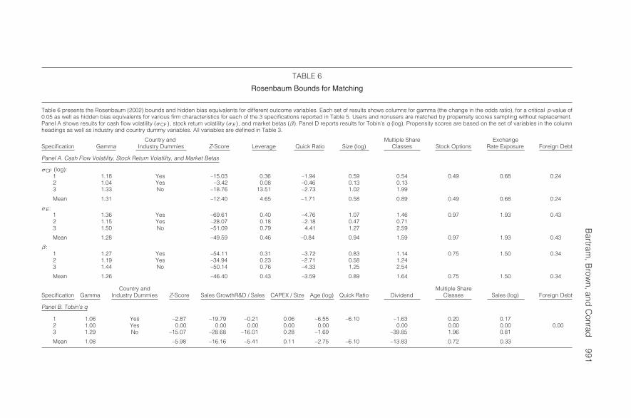
Bartram
,Brow
n,andC
onrad991
TABLE 6
Rosenbaum Bounds for Matching
Table 6 presents the Rosenbaum (2002) bounds and hidden bias equivalents for different outcome variables. Each set of results shows columns for gamma (the change in the odds ratio), for a critical p-value of0.05 as well as hidden bias equivalents for various firm characteristics for each of the 3 specifications reported in Table 5. Users and nonusers are matched by propensity scores sampling without replacement.Panel A shows results for cash flow volatility (σCF), stock return volatility (σE), and market betas (β). Panel D reports results for Tobin’s q (log). Propensity scores are based on the set of variables in the columnheadings as well as industry and country dummy variables. All variables are defined in Table 3.
Country and Multiple Share ExchangeSpecification Gamma Industry Dummies Z-Score Leverage Quick Ratio Size (log) Classes Stock Options Rate Exposure Foreign Debt
Panel A. Cash Flow Volatility, Stock Return Volatility, and Market Betas
σCF (log):1 1.18 Yes –15.03 0.36 –1.94 0.59 0.54 0.49 0.68 0.242 1.04 Yes –3.42 0.08 –0.46 0.13 0.133 1.33 No –18.76 13.51 –2.73 1.02 1.99
Mean 1.31 –12.40 4.65 –1.71 0.58 0.89 0.49 0.68 0.24
σE:1 1.36 Yes –69.61 0.40 –4.76 1.07 1.46 0.97 1.93 0.432 1.15 Yes –28.07 0.18 –2.18 0.47 0.713 1.50 No –51.09 0.79 4.41 1.27 2.59
Mean 1.28 –49.59 0.46 –0.84 0.94 1.59 0.97 1.93 0.43
β:1 1.27 Yes –54.11 0.31 –3.72 0.83 1.14 0.75 1.50 0.342 1.19 Yes –34.94 0.23 –2.71 0.58 1.243 1.44 No –50.14 0.76 –4.33 1.25 2.54
Mean 1.26 –46.40 0.43 –3.59 0.89 1.64 0.75 1.50 0.34
Country and Multiple ShareSpecification Gamma Industry Dummies Z-Score Sales GrowthR&D / Sales CAPEX / Size Age (log) Quick Ratio Dividend Classes Sales (log) Foreign Debt
Panel B. Tobin’s q
1 1.06 Yes –2.87 –19.79 –0.21 0.06 –6.55 –6.10 –1.63 0.20 0.172 1.00 Yes 0.00 0.00 0.00 0.00 0.00 0.00 0.00 0.00 0.003 1.29 No –15.07 –28.68 –16.01 0.28 –1.69 –39.85 1.96 0.81
Mean 1.08 –5.98 –16.16 –5.41 0.11 –2.75 –6.10 –13.83 0.72 0.33

992 Journal of Financial and Quantitative Analysis
slightly more sensitive to selection bias. For example, in specification 2 if usersare only about 5% more likely to possess some hidden characteristic that is asso-ciated with derivative use, the inferences could be overturned. In the remainingspecifications, the magnitude of the hidden bias is large and roughly comparableto those estimated for total risk. The average gammas and sensitivities are com-parable to those for total risk and systematic risk.24
Finally, the results with respect to the value premium appear to be even moresensitive to hidden bias, using most of the propensity score matching techniques.For example, specification 2 shows that inferences are potentially overturned atany level of bias.25 Consequently, the effect of derivative use on market value ishighly affected by even a small degree of selection bias in the sample. The sensi-tivity of the value differential associated with derivative use to selection bias mayexplain the mixed results in the literature. This result suggests that the estimatedvalue premium (or discount) may be heavily dependent on the sample, the controlvariables used, and the specification method employed in the tests. At a minimum,these results suggest that the inference that hedging increases firm value shouldbe treated very cautiously.
3. Robustness Checks
We conduct a series of robustness checks on our results. As a robustnesscheck on the matching results, we use the same binary variable to measure deriva-tive use, and estimate a treatment effects model as in Heckman (1979). We findsimilar results: Derivative use is associated with significantly lower measures ofrisk. Likewise, the relation of derivative use to Tobin’s q is significantly positive.We also use a measure of derivative use intensity, rather than merely derivativeuse, as the variable of interest, as well as an instrumental variables technique tomeasure the effect of derivative use on the firm.26 The results are similar in sign,but weaker in statistical significance. The use of a broader array of derivative con-tracts is associated with lower cash flow volatility; the results for idiosyncraticvolatility and systematic risk are negative, but not statistically significant, whilethe relation between additional contract use and relative market value is positivebut not statistically significant. This indicates that the documented differences inrisk and value are more strongly associated with any use of derivatives rather thanthe extent of use of derivatives. In turn, this may suggest that derivative use servesas a proxy for broader financial risk management policies.27
24In some cases, the change in the independent variable that would be required to overturn thebounds is not physically possible. For example, consider the change in the Z-score column wherelarge negative changes (e.g., 15.03, observed in row 1) would not be observable. This suggests that theinferences about the effect of derivative use on risk could not be overturned by any possible changein this measure of financial distress. Of course, this does not imply that another, omitted variable maynot be important, but this variable must be unrelated to the Z-score.
25Note that the p-value is above the critical value at a gamma level of 1.0. Recall that in thisspecification of the propensity score matching, the difference in Tobin’s q across users and nonusersis not significant (see Table 5).
26From these binary variables, we create a variable equal to the sum of the categories for which wedocument firms using derivatives. For example, a firm that uses exchange rate forwards, exchange rateoptions, and interest rate swaps would have a hedging intensity of 3.
27Related to this test, we examined differences in the risk measures of firms that use only interestrate derivatives and firms that used interest rate derivatives along with some other contract(s). Since

Bartram, Brown, and Conrad 993
Finally, we estimate a series of simultaneous equations models, similar to thespecification employed in Graham and Rogers (2002), in which derivatives useand 3 alternate measures of risk (volatility of cash flow, standard deviation, andnormalized standard deviation of returns) are dependent variables in a system of2 equations that include other control variables. In untabulated results (availablefrom the authors), we continue to find that derivative use is associated with adecline in the volatility of all 3 measures of risk, with p-values on the coefficientassociated with derivative use ranging from 0.03 to 0.06.
These models also have the advantage that we can estimate the effects ofother variables on firm risk and value after accounting for the use of derivatives.We find that line-of-business diversification, dividend payout, and profitabilitytend to be negatively related to σCF, σE, and β; leverage is positively related toσE and negatively related to σCF and β, whereas Gross-FX-Exposure is usuallypositively related to all 3 measures. Interestingly, firm size is positively related toσCF and β, but not a significant determinant of σE. For q we find that firm size,dividend payout, R&D expenditures, and leverage have negative coefficients, andprofitability has a positive coefficient. We find no evidence of a diversificationdiscount (i.e., the coefficient on the number of industry segments variable is notstatistically significant). The result for R&D expenditures is somewhat surprisingbut may be the result of the sample period when tech companies with high R&Dspending had low market returns.
Overall, the results from using alternative measures of derivative use, as wellas different methods, are consistent with those presented previously: The use ofderivatives by firms is associated with a significant decline in risk, while effectson value tend to be positive but statistically weaker.
C. Time-Series Evidence
As noted already, our sample period encompasses a period of economic de-cline and a sharp market correction. During 2001, the majority of countries in oursample experienced a significant economic downturn with many experiencing arecession. For example, the United States experienced a recession from March2001 through November 2001 and a so-called “jobless recovery” for more thanthe next 12 months. Global equity markets also declined sharply in this period,with the U.S. markets experiencing decline in each year from 2000 to 2002. Theeconomic and financial dislocation led to an uptick in corporate bankruptcies aswell as a drastic decline in new and seasoned equity issuances.28 Consequently, ifone goal of financial risk management with derivatives is to lower the probability
interest rate derivatives by themselves should not affect operating cash flows (only net income), anydifferences in the volatility of operating cash flow should be attributable to the direct effects of (other)hedging on risk. In matching tests, however, there is no significant difference between firms that useonly interest derivatives and those that use more extensive derivative contracts. This is consistent with(any) derivative use serving as a proxy for a host of risk management strategies employed by the firm,rather than specific derivative contracts each having a discretely measurable effect on different risksborne by the firm.
28For example, data provided by Jay Ritter (http://bear.cba.ufl.edu/ritter/publ papers/IPOALL.xls)show that the number of initial public offerings in the United States declined from 505 in 1999 to only84 in 2001.

994 Journal of Financial and Quantitative Analysis
of financial distress, then firms that manage risk may have experienced significantbenefits during this period.
We examine this hypothesis by calculating the time series of annual differ-ences in adjusted risk measures (1998–2003) for firms in our sample that use, anddo not use, derivatives. We compute these differences only across the subsamplesof firms for which sufficient data are available. Since several additional years ofdata are necessary to calculate cash flow volatility, we omit this variable from ouranalysis. We assume that derivative use is constant over this time period and soclassify firms as users or nonusers over the entire period.29
Table 7 reports the results of this analysis using the matched sample methodpresented in Table 5; for brevity, we report results for only 1 matching specifica-tion (specification 1 in previous tables). In Panel A, we present the time series of2 risk measures, σE and β. Results for σE show that derivative users have lowertotal risk in each year (at better than the 0.001 significance level). The differencein 2000 is the largest but does not stand out. Results for β also show consistentlylower levels of risk for derivative users. The results are fairly stable across years,with the differences for 2000 and 2001 only slightly higher than the average ofall years. The economic significance of these results is similar to that observed inTable 5.
Although we observe consistently lower levels of risk for derivative usersthroughout our sample period, lower risk may add more value in times of financialor economic declines. To examine this possibility, Panel B of Table 7 presents 2measures of value: annual differences in Tobin’s q, and measures of alpha (αj)from our estimates of equation (1).
Measured by Tobin’s q, the only year with a statistically significant premium(at the 10% confidence level) is 2001 (a year that witnessed both the slowestglobal gross domestic product (GDP) growth in over a decade and a recession inthe United States). When we examine differences in matched alphas each year,users experience significantly higher alphas than nonusers in each year except1998. The positive difference in 2000 is the largest in the sample period and iseconomically quite large (5.9%) compared to the average difference across allyears (2%).
Panel C of Table 7 presents the time series of various measures of profitabil-ity, including ROA, cash flow, and earnings yield. For each measure, profits aresignificantly higher (at the 10% confidence level) for derivative users in 2000through 2002. Just as importantly, the better profitability of derivative users isdue to more stable profits over this 6-year period, with nonusers exhibiting muchsharper declines from 2000 to 2001 than derivative users. For example, ROA de-clines for derivative users from 0.064 in 2000 to 0.033 in 2001, a drop of about50%, while it declines by approximately 75% for nonusers. Cash flow declinesby 0.015 from 2000 to 2001 for firms that use derivatives (or approximately 14%)and by 0.028 (or about 30%) for nonusers in the same period. Earnings yield fornonusers shows evidence of a decline earlier than derivative users: Earnings in
29To evaluate the validity of this assumption, we examined the use of a random sample of 50 usersand 50 nonusers in 1998 and 2003. Of the firms with available data, 84% of the nonusers and 82% ofthe users followed the same strategy in 1998 and 2003 as in 2000–2001.

Bartram, Brown, and Conrad 995
TABLE 7
Matched-Sample Tests of Corporate Risk Measures and Derivatives Use across Time
Table 7 presents the mean value of risk measures (Panel A), value measures (Panel B), and profit measures (Panel C) byyear for derivative users and nonusers based on propensity score matched samples. The p-values are from Wilcoxon ranksum tests between derivative users and nonusers. Results are shown for matching by year with replacement using thematching options “caliper (0.01) trim(1) common.” The following variables are used as explanatory variables of derivativesusage. For stock return volatility, market betas, and profit measures: Z-score, leverage, quick ratio, size (log), multipleshare classes, stock options, gross exchange rate exposure, foreign debt, and industry and country dummy variables;for Tobin’s q and Alpha: Z-score, sales growth, R&D / size, CAPEX / size, age (log), quick ratio, sales (log), dividend(dummy), multiple share classes, stock options, gross exchange rate exposure, foreign debt, and industry and countrydummy variables. All variables are defined in Table 3.
Variable 1998 1999 2000 2001 2002 2003
Panel A. Risk Measures
σE:User 0.430 0.422 0.483 0.460 0.443 0.372Nonuser 0.455 0.456 0.525 0.479 0.467 0.411Difference –0.025 –0.034 –0.042 –0.019 –0.024 –0.039
p-value <0.001 <0.001 <0.001 <0.001 <0.001 <0.001
β:User 0.698 0.505 0.576 0.694 0.702 0.736Nonuser 0.792 0.580 0.686 0.814 0.806 0.847Difference –0.094 –0.075 –0.110 –0.120 –0.104 –0.111
p-value <0.001 <0.001 <0.001 <0.001 <0.001 <0.001
Panel B. Value Measures
q:User 0.567 0.564 0.507 0.435 0.287 0.434Nonuser 0.558 0.577 0.593 0.392 0.267 0.471Difference 0.009 –0.013 –0.086 0.043 0.020 –0.037
p-value 0.560 0.071 0.001 0.071 0.152 0.001
Alpha (annualized):User –0.149 –0.010 –0.029 –0.003 –0.061 0.142Nonuser –0.088 –0.045 –0.088 –0.018 –0.102 0.110Difference –0.061 0.035 0.059 0.015 0.041 0.032
p-value <0.001 0.004 <0.001 0.047 <0.001 0.007
Panel C. Profit Measures
Return on Assets (ROA):User 0.063 0.066 0.064 0.033 0.015 0.031Nonuser 0.055 0.062 0.060 0.015 –0.006 0.029Difference 0.008 0.004 0.004 0.018 0.021 0.002
p-value 0.045 0.364 0.070 <0.001 <0.001 0.548
Cash Flow:User 0.108 0.112 0.108 0.093 0.091 0.099Nonuser 0.087 0.105 0.093 0.065 0.050 0.073Difference 0.021 0.007 0.015 0.028 0.041 0.026
p-value <0.001 0.415 <0.001 <0.001 <0.001 <0.001
Earnings Yield:User 0.026 0.037 0.031 –0.016 –0.036 –0.006Nonuser 0.005 0.028 –0.002 –0.049 –0.080 –0.003Difference 0.021 0.009 0.033 0.033 0.044 –0.003
p-value <0.001 0.012 <0.001 <0.001 <0.001 0.184
2000 for firms that do not use derivatives are essentially 0. And, the decline inearnings from 1999 through 2001 for derivative users, at –5.3%, is smaller thanfor nonusers, at –7.7%.
Taken as a whole, these results suggest important time variation in a firm’srisk and value measures related to financial or economic conditions. In particular,it appears that derivative use is more valuable during market downturns. To ex-amine this possibility further, we condition our analysis on broad market returnsin a firm’s home country. Specifically, we create 2 equal-weighted portfolios that
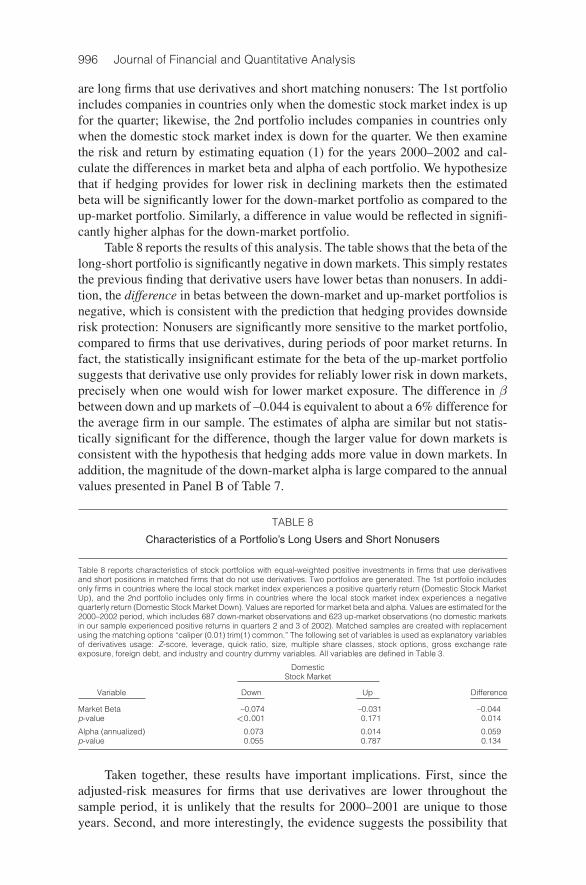
996 Journal of Financial and Quantitative Analysis
are long firms that use derivatives and short matching nonusers: The 1st portfolioincludes companies in countries only when the domestic stock market index is upfor the quarter; likewise, the 2nd portfolio includes companies in countries onlywhen the domestic stock market index is down for the quarter. We then examinethe risk and return by estimating equation (1) for the years 2000–2002 and cal-culate the differences in market beta and alpha of each portfolio. We hypothesizethat if hedging provides for lower risk in declining markets then the estimatedbeta will be significantly lower for the down-market portfolio as compared to theup-market portfolio. Similarly, a difference in value would be reflected in signifi-cantly higher alphas for the down-market portfolio.
Table 8 reports the results of this analysis. The table shows that the beta of thelong-short portfolio is significantly negative in down markets. This simply restatesthe previous finding that derivative users have lower betas than nonusers. In addi-tion, the difference in betas between the down-market and up-market portfolios isnegative, which is consistent with the prediction that hedging provides downsiderisk protection: Nonusers are significantly more sensitive to the market portfolio,compared to firms that use derivatives, during periods of poor market returns. Infact, the statistically insignificant estimate for the beta of the up-market portfoliosuggests that derivative use only provides for reliably lower risk in down markets,precisely when one would wish for lower market exposure. The difference in βbetween down and up markets of –0.044 is equivalent to about a 6% difference forthe average firm in our sample. The estimates of alpha are similar but not statis-tically significant for the difference, though the larger value for down markets isconsistent with the hypothesis that hedging adds more value in down markets. Inaddition, the magnitude of the down-market alpha is large compared to the annualvalues presented in Panel B of Table 7.
TABLE 8
Characteristics of a Portfolio’s Long Users and Short Nonusers
Table 8 reports characteristics of stock portfolios with equal-weighted positive investments in firms that use derivativesand short positions in matched firms that do not use derivatives. Two portfolios are generated. The 1st portfolio includesonly firms in countries where the local stock market index experiences a positive quarterly return (Domestic Stock MarketUp), and the 2nd portfolio includes only firms in countries where the local stock market index experiences a negativequarterly return (Domestic Stock Market Down). Values are reported for market beta and alpha. Values are estimated for the2000–2002 period, which includes 687 down-market observations and 623 up-market observations (no domestic marketsin our sample experienced positive returns in quarters 2 and 3 of 2002). Matched samples are created with replacementusing the matching options “caliper (0.01) trim(1) common.” The following set of variables is used as explanatory variablesof derivatives usage: Z-score, leverage, quick ratio, size, multiple share classes, stock options, gross exchange rateexposure, foreign debt, and industry and country dummy variables. All variables are defined in Table 3.
DomesticStock Market
Variable Down Up Difference
Market Beta –0.074 –0.031 –0.044p-value <0.001 0.171 0.014
Alpha (annualized) 0.073 0.014 0.059p-value 0.055 0.787 0.134
Taken together, these results have important implications. First, since theadjusted-risk measures for firms that use derivatives are lower throughout thesample period, it is unlikely that the results for 2000–2001 are unique to thoseyears. Second, and more interestingly, the evidence suggests the possibility that

Bartram, Brown, and Conrad 997
derivative use primarily lowers downside risk.30 Third, if part of the risk reductionfrom derivative use comes from limiting exposure to financial or economic down-turns, this provides a direct mechanism for understanding why derivative useaffects market value. Specifically, if derivative use lowers a firm’s business-cyclerisk, this may lead to a lower market beta, a lower discount rate, and therefore ahigher firm value.
VI. Conclusion
In this paper, we use a large sample of firms operating in 47 countries toanalyze the effect of derivative use on measures of risk and value. In univariatetests, we find that derivative use is more prevalent in firms with higher exposuresto interest rate risk, exchange rate risk, and commodity prices. Despite higherexposures, firms that use derivatives have lower estimated values of both total andsystematic risk, suggesting that derivatives are used to hedge risk, rather than tospeculate. There are significant differences between derivative users and nonusersalong other dimensions, emphasizing the importance of multivariate tests.
Our primary multivariate test uses propensity score matching, in whichderivative users and nonusers are matched on the basis of their (estimated) propen-sity to use derivatives. In robustness checks, we employ 2 other types of multi-variate tests. Using each method, we find that compared to firms that do not usederivatives, derivative users have lower cash flow volatility, idiosyncratic volatil-ity, and systematic risk; these results are robust to a number of different matchingspecifications, and the differences are both statistically and economically signif-icant. This suggests that nonfinancial firms overall employ derivatives with themotive and effect of risk reduction. Consistent with the evidence in Allayannisand Weston (2001), derivative use is associated with a value premium, althoughthe statistical significance of this premium is weak.
We also estimate the potential importance of selection bias on the inferencesdrawn from our tests, by estimating bounds beyond which the inferences wouldchange. These results suggest that the estimated effects of derivative use on riskmeasures are robust: While we cannot rule out the possibility that selection biasis driving our results, any omitted control variable would have to be quite signif-icant in its effect on risk to overturn the inference that the risk of firms that usederivatives is lower. In contrast, the value effects of derivative use are quite sensi-tive to selection bias. This result may explain the differences in inferences in theliterature; even small differences in sample construction, control variables, andtesting method could change the estimated effect.
Finally, we document that the reductions in risk we find are unlikely to bespecific to our primary sample period; however, we do find that market betas vary
30Interestingly, it appears to be downside risk, and not total financial risk, that is lower for firmsthat use derivatives. In a separate analysis, we examined the difference in the Altman’s Z-scores ofderivative users and matching nonusers for surviving firms in the 4 years after a firm was classified as a“user” or “nonuser” (in 2000 or 2001). We find that derivative users have a significantly lower Z-scorein every year from 2002 to 2005. This suggests that firms that use derivatives typically have higherfinancial risk. We thank the referee for this suggestion; these results are available from the authors.

998 Journal of Financial and Quantitative Analysis
in a way that is consistent with firms hedging downside risk. Lower betas may in-dicate that hedging has an effect on a firm’s cost of capital and thus the investmentpolicy and economic profitability of a firm. This in turn may explain why someof our evidence indicates that users have higher values and risk-adjusted marketreturns.
In further analyses, we explore whether firms’ access to derivative markets,or type of derivative use, influences the effects of derivatives on firms’ risk andvalue. We find relatively little evidence that the effects of derivatives vary acrossthese measures. Although this may suggest that proposed new derivative ruleswill not prevent firms from capturing the benefits of risk management, our resultsshould be interpreted with caution. In our judgment, the cross-sectional differ-ences in derivative type and access in our sample are too small, and the estimatesof the benefits of derivative use on risk are too large, to make that claim with thisevidence.
ReferencesAlkeback, P., and N. Hagelin. “Derivative Usage by Nonfinancial Firms in Sweden with an Interna-
tional Comparison.” Journal of International Financial Management and Accounting, 10 (1999),105–120.
Allayannis, Y., and E. Ofek. “Exchange Rate Exposure, Hedging, and the Use of Foreign CurrencyDerivatives.” Journal of International Money and Finance, 20 (2001), 273–296.
Allayannis, Y., and J. P. Weston. “The Use of Foreign Currency Derivatives and Firm Market Value.”Review of Financial Studies, 14 (2001), 243–276.
Altman, E. I. “Financial Ratios, Discriminant Analysis and the Prediction of Corporate Bankruptcy.”Journal of Finance, 4 (1968), 589–609.
Aretz, K., and S. M. Bartram. “Corporate Hedging and Shareholder Value.” Journal of FinancialResearch, 33 (2010), 317–371.
Bank for International Settlements. “Triennial Central Bank Survey of Foreign Exchange and Deriva-tives Market Activity in 2004” (2005).
Bartram, S. M. “Corporate Risk Management as a Lever for Shareholder Value Creation.” FinancialMarkets, Institutions and Instruments, 9 (2000), 279–324.
Bartram, S. M.; G. W. Brown; and F. R. Fehle. “International Evidence on Financial DerivativesUsage.” Financial Management, 38 (2009), 185–206.
Bartram, S. M.; G. W. Brown; and R. M. Stulz. “Why Are U.S. Stocks More Volatile?” Journal ofFinance, forthcoming (2011).
Berkman, H.; M. E. Bradbury; and S. Magan. “An International Comparison of Derivatives Use.”Financial Management, 26 (1997), 69–73.
Bodnar, G. M.; A. de Jong; and V. Macrae. “The Impact of Institutional Differences on Derivatives Us-age: A Comparative Study of U.S. and Dutch Firms.” European Financial Management, 9 (2003),271–297.
Bodnar, G. M., and G. Gebhardt. “Derivatives Usage in Risk Management by U.S. and German Non-Financial Firms: A Comparative Survey.” Journal of International Financial Management andAccounting, 10 (1999), 153–187.
Bodnar, G. M.; G. S. Hayt; and R. C. Marston. “1995 Wharton Survey of Derivatives Usage by U.S.Non-Financial Firms.” Financial Management, 25 (1996), 113–133.
Bodnar, G. M.; G. S. Hayt; and R. C. Marston. “1998 Wharton Survey of Financial Risk Managementby U.S. Non-Financial Firms.” Financial Management, 27 (1998), 70–91.
Bodnar, G. M.; G. S. Hayt; R. C. Marston; and C. W. Smithson. “Wharton Survey of DerivativesUsage by U.S. Non-Financial Firms.” Financial Management, 24 (1995), 104–114.
Brown, G. W.; P. R. Crabb; and D. Haushalter. “Are Firms Successful at Selective Hedging?” Journalof Business, 79 (2006), 2925–2949.
DeCeuster, M. J. K.; E. Durinck; E. Laveren; and J. Lodewyckx. “A Survey into the Use of Derivativesby Large Non-Financial Firms Operating in Belgium.” European Financial Management, 6 (2000),301–318.
DeMarzo, P. M., and D. Duffie. “Corporate Incentives for Hedging and Hedge Accounting.” Reviewof Financial Studies, 8 (1995), 743–771.

Bartram, Brown, and Conrad 999
DiPrete, T. A., and M. Gangl. “Assessing Bias in the Estimation of Causal Effects: Rosenbaum Boundson Matching Estimators and Instrumental Variables Estimation with Imperfect Instruments.” Soci-ological Methodology, 34 (2004), 271–310.
Downie, D.; J. McMillan; and E. Nosal. “The University of Waterloo Survey of Canadian DerivativesUse and Hedging Activities.” In Managing Financial Risk, Yearbook 1996, C. W. Smithson, ed.New York: CIBC-Wood Grundy (1996).
Froot, K. A.; D. S. Scharfstein; and J. C. Stein. “Risk Management: Coordinating Corporate Invest-ment and Financing Policies.” Journal of Finance, 48 (1993), 1629–1658.
Geczy, C.; B. A. Minton; and C. Schrand. “Why Firms Use Currency Derivatives.” Journal of Finance,52 (1997), 1323–1354.
Graham, J. R., and D. A. Rogers. “Do Firms Hedge in Response to Tax Incentives?” Journal ofFinance, 57 (2002), 815–839.
Graham, J. R., and C. W. Smith, Jr. “Tax Incentives to Hedge.” Journal of Finance, 54 (1999), 2241–2262.
Grant, K., and A. P. Marshall. “Large UK Companies and Derivatives.” European Financial Manage-ment, 3 (1997), 191–208.
Guay, W. R. “The Impact of Derivatives on Firm Risk: An Empirical Examination of New DerivativeUsers.” Journal of Accounting and Economics, 26 (1999), 319–351.
Guay, W., and S. P. Kothari. “How Much Do Firms Hedge with Derivatives?” Journal of FinancialEconomics, 70 (2003), 423–461.
Haushalter, G. D. “Financing Policy, Basis Risk, and Corporate Hedging: Evidence from Oil and GasProducers.” Journal of Finance, 55 (2000), 107–152.
Heckman, J. J. “Sample Selection as a Specification Error.” Econometrica, 47 (1979), 153–161.Hentschel, L., and S. P. Kothari. “Are Corporations Reducing or Taking Risks with Derivatives?”
Journal of Financial and Quantitative Analysis, 36 (2001), 93–118.Jin, Y., and P. Jorion. “Firm Value and Hedging: Evidence from U.S. Oil and Gas Producers.” Journal
of Finance, 61 (2006), 893–919.Koski, J. L., and J. Pontiff. “How Are Derivatives Used? Evidence from the Mutual Fund Industry.”
Journal of Finance, 54 (1999), 791–816.Leland, H. E. “Agency Costs, Risk Management, and Capital Structure.” Journal of Finance, 53
(1998), 1213–1243.Loderer, C., and K. Pichler. “Firms, Do You Know Your Currency Risk Exposure? Survey Results.”
Journal of Empirical Finance, 7 (2000), 317–344.Mian, S. L. “Evidence on Corporate Hedging Policy.” Journal of Financial and Quantitative Analysis,
31 (1996), 419–439.Modigliani, F., and M. H. Miller. “The Cost of Capital, Corporation Finance, and the Theory of
Investment.” American Economic Review, 48 (1958), 261–297.Nance, D. R.; C. W. Smith, Jr.; and C. W. Smithson. “On the Determinants of Corporate Hedging.”
Journal of Finance, 48 (1993), 267–284.Newey, W. K., and K. D. West. “A Simple, Positive Semi-Definite, Heteroskedasticity and Autocorre-
lation Consistent Covariance Matrix.” Econometrica, 55 (1987), 703–708.Rosenbaum, P. R. Observational Studies, 2nd ed. New York, NY: Springer-Verlag (2002).Rosenbaum, P. R., and D. B. Rubin. “The Central Role of the Propensity Score in Observational
Studies for Causal Effects.” Biometrika, 70 (1983), 41–55.Rountree, B.; J. P. Weston; and G. Allayannis. “Do Investors Value Smooth Performance?” Journal
of Financial Economics, 90 (2008), 237–251.Sheedy, E. “Corporate Use of Derivatives in Hong Kong and Singapore: A Survey.” Working Paper,
Macquarie University (2002).Smith, C. W., and R. M. Stulz. “The Determinants of Firms’ Hedging Policies.” Journal of Financial
and Quantitative Analysis, 20 (1985), 391–405.Stulz, R. M. “Optimal Hedging Policies.” Journal of Financial and Quantitative Analysis, 19 (1984),
127–140.Tufano, P. “Who Manages Risk? An Empirical Examination of the Risk Management Practices in the
Gold Mining Industry.” Journal of Finance, 51 (1996), 1097–1137.Zhao, Z. “Using Matching to Estimate Treatment Effects: Data Requirements, Matching Metrics, and
Monte Carlo Evidence.” Review of Economics and Statistics, 86 (2004), 91–107.