Marquette Universitye-Publications@Marquette

Economics Faculty Research and Publications Economics, Department of

9-1-2016

Effects of Foreign Direct Investment on Firm-levelTechnical Efficiency: Stochastic Frontier ModelEvidence from Chinese Manufacturing FirmsMiao Grace WangMarquette University, grace.wang@marquette.edu

Sunny WongUniversity of San Francisco

Accepted version. Atlantic Economic Journal, Vol. 44, No. 3 (September 2016): 335-361. DOI. ©2016 International Atlantic Economic Society. Used with permission.Shareable Link. Provided by the Springer Nature SharedIt content-sharing initiative.

Marquette University

e-Publications@Marquette

Economics Faculty Research and Publications/College of Business Administration

This paper is NOT THE PUBLISHED VERSION; but the author’s final, peer-reviewed manuscript. The published version may be accessed by following the link in the citation below.

Atlantic Economics Journal, Vol. 44, No. 3 (September 2016): 335-361. DOI. This article is © Springer and permission has been granted for this version to appear in e-Publications@Marquette. Springer does not grant permission for this article to be further copied/distributed or hosted elsewhere without the express permission from Springer.

Effects of Foreign Direct Investment on Firm-level Technical Efficiency: Stochastic Frontier Model Evidence from Chinese Manufacturing Firms

Miao Wang Department of Economics, University of San Francisco, San Francisco, CA M.C. Sunny Wong Department of Economics, University of San Francisco, San Francisco, CA

Abstract It has been recognized that multinational corporations can spill over to non-affiliated firms in host

economies. Existing studies of foreign direct investment (FDI) and productivity growth often assume firms are perfectly efficient. Our paper relaxes this assumption and explores how FDI affects a firm’s technical efficiency improvement as well as its technical progress in a stochastic frontier model. The stochastic frontier model

estimates a firm’s production frontier given a set of production inputs. The deviation of a firm’s actual output level from its maximum level of output is defined as technical inefficiency. Using data from more than 12,000 Chinese manufacturing firms, we find that FDI in a firm's own industry (horizontal FDI) does not necessarily improve the firm’s technical efficiency. However, firms with a larger absorptive capacity tend to benefit more from horizontal FDI than others. We also find that foreign presence in a firm’s downstream industries helps improve the firm’s technical efficiency, while foreign presence in upstream industries does not. In addition, a generalized Malmquist index decomposition shows that foreign affiliates achieve a higher productivity growth than domestic firms mainly through a faster improvement in technical efficiency rather than through technical progress.

Keywords Foreign direct investment, Horizontal and vertical spillovers, Technical efficiency, Stochastic frontier model, Malmquist productivity index

Introduction Foreign direct investment (FDI) is typically taken as a vehicle transferring both tangible and intangible

assets such as better product designs or management skills. The superior technology owned by multinational corporations (MNCs), which is not generally available in the host country, can spill over to non-affiliated firms and create a beneficial impact on productivity in the host country. As a result, many countries consider FDI an integral part of their development strategy and try to attract such investments by offering preferential policies to MNCs including tax breaks or subsidies. Not surprisingly, studies on FDI spillovers received tremendous attention from both academic researchers and policy makers. Since the pioneering paper of Caves (1974), there has been a large body of research exploring FDI spillovers and firm productivity in host countries (for example, Aitken and Harrison 1999; Javorcik 2004; Driffield 2004; Merlevede et al. 2014).

In this paper, we examine FDI productivity spillovers in the host country using a stochastic frontier model. Our study contributes to the literature in two respects. First, we identify the contribution of technical efficiency improvement and technical progress to productivity growth. Generally speaking, productivity growth includes two components: technical progress and technical efficiency improvement. Technical progress refers to an outward shift of the current production frontier, often caused by advances in technology. Technical efficiency improvement refers to a movement from current output level toward the production frontier. Earlier studies on FDI spillovers with industry- or firm-level data typically construct an estimate of total factor productivity (TFP), based on the Solow residual parametric or semi-parametric approaches developed by Olley and Pakes (1996) and Levinsohn and Petrin (2003). Then the impact of FDI on TFP or TFP growth is evaluated. These studies have greatly advanced our understanding of FDI spillovers. However, there are a few potential caveats with them. The first is that they do not distinguish between technical progress and technical efficiency improvement. In other words, all firms are assumed to be perfectly efficient and operate on their production frontier. Practically, firms are not always exhibiting full efficiency and there are likely (large) differences in technical efficiency across firms. In addition, given this full efficiency assumption, the productivity externalities of FDI (if any) captured in earlier studies are purely regarded as technical progress, that is, an outward shift of the current production frontier.

In our paper, we use a stochastic frontier (SF) model to explore the extent to which foreign ownership of a firm and foreign presence at the industry level affect the firm’s productivity and efficiency. The novelties of the SF methodology are that it relaxes the strict assumption that all firms are fully efficient, identifies which

firms are inefficient and to what extent they are inefficient, and estimates sources of technical inefficiency. Consequently, we are able to calculate separately efficiency improvement, technical progress, as well as scale efficiency change, which present a more detailed picture of productivity growth. Further, in Dunning’s OLI framework (Dunning 1977), the ownership advantages of MNCs refer to advantages MNCs have from all intangible assets including both better technology (e.g. existing patents) and better management and marketing skills. Different MNCs intangible assets may have different effects on firm productivity in the host country. The SF approach helps to illustrate the productivity externalities of FDI in the host country from diffusion of newer and better technology (which leads to technical progress) and from transfer of knowledge related to better managerial and organizational practices (which improves efficiency). In contrast, the latter cannot be identified by using the traditional approach of regressing the Solow residual TFP estimate on various factors when all firms are assumed to be fully efficient.

Second, we add to the small literature on FDI presence and firm-level efficiency gains and evaluate the effect of both intra- and inter-industry FDI spillovers. Intra-industry FDI (also referred to as horizontal FDI) is FDI received in a firm’s own industry while inter-industry FDI (vertical FDI) is FDI received in a firm’s upstream or downstream industries. Existing research adopting the stochastic frontier approach with firm-level data primarily focuses on the association between foreign ownership of a firm and the firm’s technical efficiency (Oczkowski and Sharma 2005; Yaşar and Paul 2009; Hanousek et al. 2012; Charoenrat and Harvie 2014). Potential effects of FDI at the industry level are routinely left unexamined. A few exceptions include Kathuria (2001) and Suyanto et al. (2009, and 2014). Kathuria (2001), with data from 368 manufacturing firms in India, finds that there are positive spillovers from foreign presence in an industry provided firms possess significant R&D capabilities.1 Suyanto et al. (2009) use data from chemical and pharmaceutical firms in Indonesia during 1988-2000 and argue that horizontal FDI has a beneficial effect on a firm’s technical efficiency. Both Kathuria (2001) and Suyanto et al. (2009) omit vertical FDI measures, hence we may not be able to draw inferences on inter-industry FDI spillovers from their results. Suyanto et al. (2014) include both measures of intra- and inter-industry FDI. With data on manufacturing firms in Indonesia over 1988-2000, the authors find evidence supporting significant vertical FDI spillovers. Because potential vertical linkages have been recognized as important channels for FDI spillovers (compounded below), we consider foreign presence in a firm’s own industry as well as in its upstream and downstream industries in our paper.

We employ comprehensive data from over 12,000 Chinese manufacturing firms in 30 two-digit industries over 2002-2004 published by the World Bank. Our results show that intra-industry FDI has a negative effect on an individual firm’s technical efficiency. But there does exist a complementarity between a firm’s R&D expenditure and intra-industry FDI. Not all firms can benefit from horizontal FDI. Yet, positive effects of horizontal FDI on technical efficiency are closely related to a firm’s capacity to absorb new technology and knowledge. We also find the presence of foreign end-users tends to improve efficiency of domestic suppliers possibly due to the fact that MNCs can help their suppliers in the host country to build production facilities and provide technical support to raise the quality of suppliers’ products. On the other hand, our results show that foreign presence in upstream industries could have an adverse effect on the level of technical efficiency of firms as end-users.

In terms of the level of technical efficiency, foreign firms are on average more efficient than domestic firms in China. Foreign firms in our sample obtain an average efficiency score of 0.56 (a maximum value of one means full efficiency), while domestic firms obtain an average efficiency score of 0.42. A generalized Malmquist index shows that both foreign and domestic firms in China have a similar rate of technical progress at 6.4% while foreign firms on average experience a faster improvement in technical efficiency than domestic firms (4.1% vs. 3.5%).

Conceptual Framework: FDI Intra- and Inter-industry Linkages Intra-Industry FDI

Conceptually, there are three main channels through which FDI can affect host country local firms in the same industry: demonstration, training of employees, and market competition. First, there may exist the “demonstration effect” when non-affiliated firms learn from multinationals and imitate their product designs, processes, and organizational innovations (Javorcik 2008). Such learning or imitation can help non-affiliated firms to upgrade their technology, and also improve their productivity. Second, the productivity enhancing effect of FDI can occur through labor turnover. The knowledge and skills provided by training programs of MNCs can benefit local firms. For instance, workers trained by multinationals may later take employment in other firms, carrying the training with them, or become entrepreneurs and start their own business (Alfaro et al. 2009; Balsvik 2011). Third, entry of foreign firms in an industry can increase competition in the host market and rising competition gives existing firms an incentive to improve their production process. This is often referred to as the “competition effect,” which can imply a productivity gain in the host country (Glass and Saggi 2002). As argued by Aitken and Harrison (1999) and Crespo and Fontoura (2007), however, negative effects can also arise due to such competition. They describe a “market stealing” effect, when foreign firms exploit their technology advantage and “steal” customers away from existing firms in the host country. With a reduced demand and smaller market share, local firms in the host country can be forced to reduce output. Their productivity could fall when the firms spread fixed costs over a smaller quantity of output. In addition, MNCs often offer a higher wage than local firms, which can raise the wage level in the host country and increase the labor cost for all firms.

Inter-Industry FDI

Some have cast doubt on the degree of intra-industry FDI spillovers given that MNCs may have strong incentives to prevent their advanced knowledge from leaking out to competitors in the host country. In comparison, beneficial impact from inter-industry FDI on local firms’ productivity may be more likely to materialize since MNCs can be motivated to provide technologies to their suppliers or customers in the host country.

Lall (1980) proposes the concept of vertical linkages, which is later formalized by, among others, Rodríguez-Clare (1996). In the case of forward linkages, MNCs in upstream industries lead to productivity improvement of firms in downstream industries. This can happen when (more productive) MNCs supply intermediate goods and machinery of a better quality to final goods producers in the host country. It can also happen when MNCs provide technical and organizational assistance to their customers so that their products will be used more effectively. However, Javorcik (2004) argues that negative forward spillovers are possible too. If an upgrade in quality of inputs sold by MNCs is associated with an increase in product prices, firms in industries which multinationals supply might experience some negative effects due to increased cost.

Backward linkages refer to spillovers from MNCs in downstream industries to their suppliers in upstream industries. Multinationals can have higher standards or more strict requirements regarding product quality and delivery. To ensure the quality of inputs they receive, MNCs may be interested in transferring technology and providing technical support to their local suppliers (Blalock and Gertler 2008). MNCs also have incentives to make the technology widely available in the supply market so that no single supplier can behave like a monopoly and raise the product price. In addition, a rising number of foreign firms in an industry can

increase the demand for intermediate products and hence allow firms in upstream industries to boost production and exploit economies of scale.

Estimation Strategy Stochastic Frontier Framework

The stochastic frontier model estimates a firm’s production frontier or the “best practice” given a set of production inputs (Aigner et al. 1977). The deviation of a firm’s actual output level from its maximum level of output is defined as the technical inefficiency. The stochastic frontier model can be expressed as:

𝐿𝐿𝐿𝐿𝑌𝑌𝑖𝑖𝑖𝑖 = 𝑥𝑥𝑖𝑖𝑖𝑖𝛽𝛽 + 𝑣𝑣𝑖𝑖𝑖𝑖 − 𝑢𝑢𝑖𝑖𝑖𝑖 , (1)

where i and t are firm and time subscripts, respectively; Y denotes the production of a firm and x is a vector of inputs (in log) such as labor and physical capital. The error term has two components: a random error, v it, and the technical inefficiency term, u it. The random error, v it, has an iid normal distribution of (0,𝜎𝜎𝑣𝑣2); the technical inefficiency term, u it, is assumed to have a normal distribution, truncated at zero, with mean μ and variance 𝜎𝜎𝑢𝑢2. Further, the mean of the distribution of technical inefficiency can be represented as a linear function of control variables:

μit = Zit𝛿𝛿 = 𝛿𝛿0 + ∑Mm=1 𝛿𝛿mzm, (2)

where Z = [Z 1,  … , Z M ] is a vector including M determinants of technical inefficiency. Kumbhakar et al. (1991) propose a single-stage maximum likelihood estimation (MLE) procedure to estimate equations (1) and (2) simultaneously, which is later extended and modified by Battese and Coelli (1995) for panel data estimation. In this context, the point estimate of technical efficiency (TE), or the ratio of a firm’s actual output to its corresponding stochastic frontier output is:

𝑇𝑇𝐸𝐸𝑖𝑖𝑖𝑖 = 𝐸𝐸[exp (−𝑢𝑢𝑖𝑖𝑖𝑖)|𝑣𝑣𝑖𝑖𝑖𝑖 − 𝑢𝑢𝑖𝑖𝑖𝑖]. (3)

The value of TE ranges between zero and one. The larger the TE, the closer a firm operates to its production frontier, with a maximum value of one indicating a firm on its production frontier.

Data and Empirical Specification

Our empirical estimation draws on data from the 2005 Investment Climate Survey conducted by the China National Bureau of Statistics for the World Bank.2 The survey includes 12,395 firms in 30 provinces, corresponding to 30 two-digit level industries in the manufacturing sector. These firms are randomly selected from all firms in their province, industry, and size categories. The 2005 Investment Climate Survey data span the period 2002-2004. We exclude firms that do not report information on production, employment, or fixed assets as well as firms with apparent data entry errors such as a negative employment. This leaves us with a total number of 36,359 observations over 2002 to 2004. A more recent World Bank survey on Chinese firms with publicly available data was conducted in 2012. We use data from the 2005 survey for our main results as its broad coverage and panel structure allow us to study technical improvements and technical progress over time. Data from the 2012 World Bank survey cover a single year’s information, the year of 2011, which we discuss in detail in the robustness checks section. Based on equations (1) and (2), we specify a flexible translog production function:

𝑙𝑙𝐿𝐿𝑌𝑌𝑖𝑖𝑖𝑖𝑖𝑖𝑖𝑖 = 𝛽𝛽𝑐𝑐 + 𝛽𝛽𝐾𝐾𝑙𝑙𝐿𝐿𝐾𝐾𝑖𝑖𝑖𝑖𝑖𝑖𝑖𝑖 + 𝛽𝛽𝐿𝐿𝑙𝑙𝐿𝐿𝐿𝐿𝑖𝑖𝑖𝑖𝑖𝑖𝑖𝑖 + 12𝛽𝛽𝐾𝐾𝐾𝐾(𝑙𝑙𝐿𝐿𝐾𝐾𝑖𝑖𝑖𝑖𝑖𝑖𝑖𝑖)2 + 1

2𝛽𝛽𝐿𝐿𝐿𝐿(𝑙𝑙𝐿𝐿𝐿𝐿𝑖𝑖𝑖𝑖𝑖𝑖𝑖𝑖)2 + 𝛽𝛽𝐾𝐾𝐿𝐿(𝑙𝑙𝐿𝐿𝐾𝐾𝑖𝑖𝑖𝑖𝑖𝑖𝑖𝑖 × 𝑙𝑙𝐿𝐿𝐿𝐿𝑖𝑖𝑖𝑖𝑖𝑖𝑖𝑖)

+𝛽𝛽𝑇𝑇𝐾𝐾(𝑇𝑇 × 𝑙𝑙𝐿𝐿𝐾𝐾𝑖𝑖𝑖𝑖𝑖𝑖𝑖𝑖) + 𝛽𝛽𝑇𝑇𝐿𝐿(𝑇𝑇 × 𝑙𝑙𝐿𝐿𝐿𝐿𝑖𝑖𝑖𝑖𝑖𝑖𝑖𝑖) + 𝛽𝛽𝑇𝑇𝑇𝑇 + 12𝛽𝛽𝑇𝑇𝑇𝑇𝑇𝑇2 + 𝑣𝑣𝑖𝑖𝑖𝑖𝑖𝑖𝑖𝑖 − 𝑢𝑢𝑖𝑖𝑖𝑖𝑖𝑖𝑖𝑖 ,

(4)

where i, j, and p are firm, industry, and province subscripts, respectively; subscript t implies time. We measure output by a firm’s real value-added; K represents physical capital and is measured by net real fixed assets of a firm; L is labor, measured by a firm’s total number of employees; and T is a time trend. Industry and provincial dummies are also included in the production function. Our baseline average inefficiency function is represented as:

μ𝑖𝑖𝑖𝑖𝑖𝑖𝑖𝑖 = 𝛿𝛿0 + ∑ 6𝑚𝑚=1 𝛿𝛿mzm,𝑖𝑖𝑖𝑖𝑖𝑖𝑖𝑖 = 𝛿𝛿0 + 𝛿𝛿1𝐹𝐹𝐹𝐹𝐹𝐹𝐹𝐹𝐹𝐹𝐹𝐹𝐿𝐿𝑖𝑖𝑖𝑖𝑖𝑖𝑖𝑖 + 𝛿𝛿2𝐴𝐴𝐹𝐹𝐹𝐹𝑖𝑖𝑖𝑖𝑖𝑖𝑖𝑖 + 𝛿𝛿3𝑆𝑆𝐹𝐹𝑆𝑆𝐹𝐹𝑖𝑖𝑖𝑖𝑖𝑖𝑖𝑖

+𝛿𝛿4𝐹𝐹𝐹𝐹𝐹𝐹𝑖𝑖𝑖𝑖𝑖𝑖𝐻𝐻𝐻𝐻𝐻𝐻𝑖𝑖 + 𝛿𝛿5𝐹𝐹𝐹𝐹𝐹𝐹𝑖𝑖𝑖𝑖𝑖𝑖𝑈𝑈𝑖𝑖 + 𝛿𝛿6𝐹𝐹𝐹𝐹𝐹𝐹𝑖𝑖𝑖𝑖𝑖𝑖𝐷𝐷𝐻𝐻𝐷𝐷𝐷𝐷,

(5)

where Foreign is a dummy variable for foreign ownership defined by at least 10% of foreign capital. Firm’s age (Age) and size (Size, measured by the log of a firm’s total employment) are also included.

The last three variables in equation (5) represent FDI in a firm’s own industry j (𝐹𝐹𝐹𝐹𝐹𝐹𝑖𝑖𝑖𝑖𝑖𝑖𝐻𝐻𝐻𝐻𝐻𝐻𝑖𝑖), its upstream (𝐹𝐹𝐹𝐹𝐹𝐹𝑖𝑖𝑖𝑖𝑖𝑖

𝑈𝑈𝑖𝑖) and downstream (𝐹𝐹𝐹𝐹𝐹𝐹𝑖𝑖𝑖𝑖𝑖𝑖𝐷𝐷𝐻𝐻𝐷𝐷𝐷𝐷) industries. Coefficients δ 4 − δ 6 capture effects of industry level FDI on a firm’s technical inefficiency. The degree of horizontal FDI, for each province p, measures foreign share of output (Output) within an industry j at time t. In other words, with θ i as the share of firm i’s equity owned by foreign investors, we obtain:

𝐹𝐹𝐹𝐹𝐹𝐹𝑖𝑖𝑖𝑖𝑖𝑖𝐻𝐻𝐻𝐻𝐻𝐻𝑖𝑖 =� 𝜃𝜃𝑖𝑖×𝑂𝑂𝑢𝑢𝑖𝑖𝑖𝑖𝑢𝑢𝑖𝑖𝑖𝑖𝑖𝑖𝑖𝑖𝑖𝑖

𝑖𝑖∈𝑖𝑖

∑𝑖𝑖∈𝑖𝑖 𝑂𝑂𝑢𝑢𝑖𝑖𝑖𝑖𝑢𝑢𝑖𝑖𝑖𝑖𝑖𝑖𝑖𝑖𝑖𝑖. (6)

The upstream FDI for any firm in industry j is measured as a weighted average of foreign share of output in upstream industries that supply industry j (Javorcik 2004):

𝐹𝐹𝐹𝐹𝐹𝐹𝑖𝑖𝑖𝑖𝑖𝑖𝑈𝑈𝑖𝑖 = � 𝑎𝑎𝑘𝑘𝑖𝑖𝐹𝐹𝐹𝐹𝐹𝐹𝑘𝑘𝑖𝑖𝑖𝑖𝐻𝐻𝐻𝐻𝐻𝐻𝑖𝑖

𝑘𝑘≠𝑖𝑖, (7)

where α kj is the share of industry k’s output supplied to industry j as inputs. Similarly, we measure the downstream FDI for any firm in industry j as a weighted average of foreign share of output in all downstream industries that are supplied by industry j:

𝐹𝐹𝐹𝐹𝐹𝐹𝑖𝑖𝑖𝑖𝑖𝑖𝐷𝐷𝐻𝐻𝐷𝐷𝐷𝐷 = � 𝜑𝜑𝑖𝑖𝑘𝑘𝐹𝐹𝐹𝐹𝐹𝐹𝑘𝑘𝑖𝑖𝑖𝑖𝐻𝐻𝐻𝐻𝐻𝐻𝑖𝑖

𝑘𝑘≠𝑖𝑖, (8)

where φ jk is the share of industry j’s output supplied to industry k as inputs. In short, the variable 𝐹𝐹𝐹𝐹𝐹𝐹𝑖𝑖𝑖𝑖𝑖𝑖

𝑈𝑈𝑖𝑖 captures foreign presence in industry j’s upstream industries in province p at time t and the variable 𝐹𝐹𝐹𝐹𝐹𝐹𝑖𝑖𝑖𝑖𝑖𝑖𝐷𝐷𝐻𝐻𝐷𝐷𝐷𝐷 foreign presence in industry j’s downstream industries in province p.

To construct FDI in upstream and downstream industries, we use the 2002 Input–Output (I-O) Table of China, published by China National Bureau of Statistics (2006). Our sample only covers firms in manufacturing industries, but α kj and φ jk are calculated based on all industries included in the I-O table. China compiles its I-

O table every five years. We choose I-O 2002 as it fits our sample span better than I-O 1997 and I-O 2007. Descriptive statistics are presented in Table 1.

Table 1. Descriptive statistics Variable No. of Obs Mean Std. Dev. Min Max Y (in million yuan) 36359 191.4661 1521.8790 0.0004 100651.7 K (in million yuan) 36359 149.8977 1705.3250 0.0009 134459.2 L (in thousand) 36359 0.8558 2.7489 0.001 135.559 Age 36359 12.7824 13.6579 1 140 Foreign (10%) 36359 0.2088 0.4064 0 1 Foreign (25%) 36359 0.2030 0.4022 0 1 R&D (in million yuan) 36359 5.3927 53.5982 0 4359.9 FDI Hori 36359 0.1900 0.2305 0 1 FDI Up 36359 0.1173 0.1491 0.00024 0.8104 FDI Down 36359 0.1152 0.1524 0.00003 0.9103

Data come from the World Bank Enterprise Survey, China 2005.

We report the average foreign share of total output by industry and by province in our sample in Table 2. In addition, we provide number of observations in each industry (province) and their corresponding shares in total number of observations. Foreign firms play an important role in the manufacturing sector in China, contributing around 21% of the total output in the manufacturing sector. In some cases, foreign production can account for the majority of an industry’s output. For example, the share of foreign output is 62.5% in electric equipment and machinery and 54% in cultural, educational and sports goods. In terms of geographical distribution, FDI in China is concentrated in coastal regions and metropolitan cities. Central and Western China receive a considerably smaller amount of FDI. For example, an average of 59.5% of output in the manufacturing sector in Guangdong province is produced by foreign firms while this number drops to a low of 1.8% in Qinghai province.

Table 2. FDI by province and industry Industry level Province

level

Industry a Share of foreign output

No. of obs.

% of total obs.

Province Share of foreign output

No. of obs.

% of total obs.

13 Food processing 19.71 2819 7.75% Coastal Region

14 Food production 17.81 714 1.96% Beijing 34.62 587 1.61% 15 Beverage industry 27.31 528 1.45% Fujian 49.28 1478 4.07% 16 Tobacco processing 0.34 137 0.38% Guangdong 59.48 2639 7.26% 17 Textile industry 17.05 2791 7.68% Hainan 14.04 285 0.78% 18 Garments and other

fibre products 34.78 611 1.68% Jiangsu 10.65 2644 7.27%

19 Garments and other fibre products

33.14 411 1.13% Liaoning 13.1 1755 4.83%

20 Timber processing 16.59 416 1.14% Shandong 10.7 2634 7.24% 21 Furniture

manufacturing 33.04 163 0.45% Shanghai 52.47 592 1.63%

22 Papermaking and paper products

14.57 692 1.90% Tianjin 46.63 585 1.61%

23 Printing and record medium reproduction

11.82 185 0.51% Zhejiang 13.9 2370 6.52%

24 Cultural, educational and sports goods

53.97 123 0.34% Central Region

25 Petroleum refining and coking

6.24 4215 1.43% Anhui 16.26 1175 3.23%

26 Raw chemical materials and chemical products

11.83 4215 11.59% Guangxi 8.28 882 2.43%

27 Medical and pharmaceutical products

14.22 1254 3.45% Hebei 15.08 2326 6.40%

28 Chemical fibre 7.41 140 0.39% Heilongjiang 5.4 847 2.33% 29 Rubber products 15.27 63 0.17% Henan 6.32 2055 5.65% 30 Plastic products 28.91 960 2.64% Hubei 13.67 2055 5.65% 31 Nonmetal mineral

products 7.77 3833 10.54% Hunan 7.06 1758 4.84%

32 Smelting and pressing of ferrous metals

7.33 1424 3.92% Inner Mongolia

28.61 583 1.60%

33 Smelting and pressing of nonferrous metals

3.98 996 2.74% Jiangxi 21.84 1476 4.06%

34 Metal products 25.73 1056 2.90% Jilin 23.46 592 1.63% 35 Ordinary machinery 17.79 3172 8.72% Shaanxi 7.57 885 2.43%

36 Special purposes equipment

10.19 1433 3.94% Western region

37 Transport equipment

14.07 2910 8.00% Chongqing 11.86 591 1.63%

39 Other electronic equipment

32.27 2548 7.01% Gansu 2.47 584 1.61%

40 Electric equipment and machinery

62.45 1745 4.80% Guizhou 7.03 596 1.64%

41 Electronic and telecommunications

52.7 180 0.50% Ningxia 4.79 588 1.62%

42 Instruments and meters

29.8 312 0.86% Qinghai 1.78 287 0.79%

43 Other manufacturing

0.02 9 0.02% Shanxi 4.06 880 2.42%

Sichuan 7.97 1461 4.02% Xinjiang 2.55 295 0.81% Yunnan 7.19 874 2.40% 20.94 (mean) 36359

(total) 100% 16.94

(mean) 36359 (total)

100%

Data come from the World Bank Enterprise Survey, China 2005. aThe two-digit industry classification are from the National Bureau of Statistics, China.

Empirical Results Foreign Ownership and Firm Characteristics

We estimate equations (4) and (5) simultaneously with a single-stage maximum likelihood estimation (MLE) procedure and report results in Table 3. The first two regressions in Table 3 are baseline regressions without measures of industry FDI. The foreign ownership dummy in regression 3.1 is defined as at least 10% of foreign capital, consistent with the definition used in the U.S. and the IMF. Starting from regression 3.2, foreign ownership is defined as at least 25% of foreign capital, which is the threshold level adopted in China. In regression 3.3, we add horizontal, upstream and downstream FDI in the inefficiency function. In regression 3.4, we include R&D expenditure as a proxy for a firm’s absorptive capacity. Regressions 3.5 and 3.6 have lagged variables in the inefficiency function.

Table 3. Production function and technical efficiency estimates Panel (a): Production function

VARIABLES

Model 3.1

Model 3.2

Model 3.3

Model 3.4

Model 3.5

Model 3.6

Coefficient

Std. err.

Coefficient

Std. err.

Coefficient

Std. err.

Coefficient

Std. err.

Coefficient

Std. err.

Coefficient

Std. err.

ln(K) 0.11225***

[0.015]

0.11224***

[0.015]

0.11409***

[0.015]

0.09959***

[0.015]

0.12890***

[0.028]

0.11377***

[0.028]

ln(L) 0.60556***

[0.031]

0.60625***

[0.031]

0.58594***

[0.030]

0.57459***

[0.028]

0.55710***

[0.048]

0.55289***

[0.047]

ln(K)^2 0.08217***

[0.003]

0.08227***

[0.003]

0.08228***

[0.003]

0.07939***

[0.003]

0.07943***

[0.048]

0.07719***

[0.003]

ln(L)^2 0.13936***

[0.012]

0.14056***

[0.012]

0.14567***

[0.012]

0.11250***

[0.010]

0.14567***

[0.014]

0.11528***

[0.013]

ln(K) × ln(L)

-0.11183***

[0.008]

-0.11224***

[0.008]

-0.10856***

[0.008]

-0.10993***

[0.008]

-0.10490***

[0.010]

-0.10894***

[0.010]

T 0.15900***

[0.051]

0.15890***

[0.051]

0.15864***

[0.051]

0.16278***

[0.050]

0.10341**

[0.042]

0.10006**

[0.042]

T^2 -0.02939

[0.023]

-0.02935

[0.023]

-0.02945

[0.023]

-0.031 [0.023]

T × ln(K)

0.00763

[0.005]

0.00763

[0.005]

0.00781

[0.005]

0.00474

[0.005]

0.00511 [0.009]

0.00258

[0.009]

T × ln(L)

-0.01245*

[0.007]

-0.01243*

[0.007]

-0.01282*

[0.007]

-0.01003

[0.007]

-0.00364 [0.014]

-0.00184

[0.014]

Constant

3.54503***

[0.078]

3.54260***

[0.078]

3.55639***

[0.078]

3.79732***

[0.079]

-0.57043***

[0.111]

3.79340***

[0.126]

Industry dummies

Yes Yes Yes Yes Yes Yes

Province dummies

Yes Yes Yes Yes Yes Yes

Panel (b): Technical inefficiency

Size -0.75360***

[0.031]

-0.75797***

[0.031]

-0.79030***

[0.030]

-0.58642***

[0.028]

-0.73116***

Age 0.01374***

[0.001]

0.01379***

[0.001]

0.01363***

[0.001]

0.01186***

[0.001]

0.01394***

Foreign

-0.47038***

[0.038]

-0.46473***

[0.038]

-0.47807***

[0.036]

-0.46225***

[0.031]

-0.48335***

FDI Hori 0.42117***

[0.061]

0.41295***

[0.058]

FDI Up 1.24734***

[0.207]

1.18774***

[0.189]

FDI Do

wn -

1.37547***

[0.198]

-1.22649***

[0.181]

RD -1.03801***

[0.085]

RD × FDIHori

-0.4558*

[0.244]

FDI Hori

(t-1) 0.36856*

** [0.069]

0.35866***

[0.066]

FDI Up

(t-1) 1.22765*

** [0.236]

1.10765***

[0.218]

FDI Do

wn(t-1) -

1.40245***

[0.227]

-1.20541***

[0.210]

RD (t-1)

-0.94385***

[0.096]

RD FDIHori (t-1)

-0.51297*

[0.306]

Constant

-0.67168***

[0.109]

-0.68754***

[0.109]

-0.76458***

[0.102]

-0.01857

[0.080]

-0.57042***

[0.111]

0.05614

[0.093]

Mean technical efficiency (TE)

0.473 0.474 0.470 0.452 0.479 0.457

Gamma

0.464 0.464 0.46 0.472 0.385 0.409

Log likelihood

-53703.473

-53708.106

-53658.737

-53054.193

-35479.637

-35120.405

Wald Chi2

22016.64

22168.31

22663.58

17880.67

15269.76 12897.14

No. of obs

36,359 36,359 36,359 36,359 24,351 24,351

Panel (c). Likelihood ratio tests on model specifications

H0: Cobb-Douglas specification

1266.55***

1270.3***

1351.62***

1145.19***

878.53***

708.83***

H0: Neutral technological change

3.10 3.09 3.28 2.00 0.37 0.10

H0: γ = δ0 = δ1 = … = 0

1189.06***

1179.79***

1278.53***

2487.62***

37636.73***

38355.20

H0: δ1 = … = 0

618.76***

609.48***

708.21***

1917.30***

804.74***

1523.21***

Standard errors in brackets. *** p<0.01, ** p<0.05, * p<0.1. RD is defined as ln(1+R&D). Data come from the World Bank Enterprise Survey, China 2005.

Table 3 has three panels, with results of the production function in panel (a), results of the mean inefficiency function in panel (b), and hypothesis testing results in panel (c). We start our discussion with panel (c), where likelihood ratio (LR) test statistics for three hypotheses are provided. First, we compare the Cobb-Douglas functional form with the translog functional form. The null hypothesis of the Cobb-Douglas functional form is rejected at the 1% level consistently across all specifications, suggesting the translog functional form is a more appropriate description of the production process. To test the “no-inefficiency” effect, we follow Battese and Coelli (1995) and define γ=σ2u/σ2γ=σu2/σ2, where σ2=σ2u+σ2vσ2=σu2+σv2. The null hypothesis is based on the joint significance of γ = δ 0 = δ 1 =  …  = 0, where δs are parameters in the inefficiency function. As shown in Table 3, the null hypothesis of no inefficiency can be rejected at the 1% level in all models. Lastly, we test whether the average inefficiency is a function of Z factors included in equation (5). The null hypothesis that all slope parameters in the inefficiency function are jointly zero (i.e., H 0 : δ 0 = δ 1 = … = 0) is rejected consistently. This suggests that control variables included in the average technical inefficiency function explain sources of the observed inefficiency.

Looking across columns in panel (b), there are a few notable points. First, the coefficient on foreign ownership (Foreign) in the technical inefficiency function is negative and statistically significant at the 1% level in all regressions. Changing the threshold level of foreign share does not alter this result. Since we are estimating an inefficiency function, a negative coefficient means a particular factor reduces technical inefficiency or raises technical efficiency. The robustly negative coefficient on foreign ownership implies foreign firms are more efficient than domestic firms. In model 3.4, the coefficient on Foreign is -0.46, suggesting that other things constant, foreign firms are 46% more efficient than domestic firms. This result is consistent with previous frontier analyses focusing on ownership and a firm’s technical efficiency. For example, Suyanto et al. (2014) also find that foreign affiliates are more efficient than domestic manufacturing firms in Indonesia.

Second, in our sample, firm age (Age) is positively associated with technical inefficiency and firm size (Size) is negatively associated with technical inefficiency. For example, the estimated coefficient on firm age in model 3.3 is 0.014 and significant at the 1% level. This suggests that older firms are less efficient or holding other things constant, a one-year increase in a firm’s age is associated with a 1.4% increase in inefficiency or a 1.4% drop in the level of technical efficiency. Our findings on firm age and technical efficiency echo findings in Charoenrat et al. (2013). Older firms may employ capital of earlier vintage while younger firms are more likely to adopt modern technology and equipment. Consequently older firms tend to be less productive or exhibit lower efficiency than younger firms. The estimated coefficient on firm size (Size) is robustly negative, indicating the larger the firm is, the closer it is to the production frontier. Regression 3.3 suggests that a 1% rise in a firm’s total employment is associated with a reduction in its inefficiency by 0.79%.

Horizontal, Downstream, and Upstream FDI and Technical Efficiency

Focusing on industry-level FDI, Table 3 shows that intra-industry FDI (FDIHori ) has a positive and significant coefficient, indicating that an increase in horizontal FDI may decrease a firm’s technical efficiency. Regression 3.3 shows that, ceteris paribus, a 1% increase in FDI in a firm’s own industry is associated with a 0.42% decline in the firm’s technical efficiency. Conceptually, the net effect of horizontal FDI in an industry could be rather ambiguous. As mentioned previously, positive spillovers from intra-industry FDI may occur through channels such as demonstration or labor turnover. In other words, non-affiliated firms learn from multinationals and imitate their product designs, processes, or organizational innovations. On the other hand, foreign presence may harm domestic firms due to “market-stealing,” when foreign entry reduces indigenous firms’ market share and forces them to reduce output and incur a higher average production cost. The

positive coefficient on the horizontal FDI in our regressions likely shows a dominant market-stealing effect of FDI over the beneficial spillover effect.

Regarding the effect of vertical FDI, the coefficient on FDI Down is negative and significant at the 1% level, suggesting foreign presence in a firm’s downstream industries tends to increase its technical efficiency. This might be caused by the higher requirements set by MNCs on the quality and delivery of inputs from local suppliers. In addition, the beneficial impact of foreign presence in a firm’s downstream industries on the firm’s technical efficiency could result from an increase in the demand for intermediate products, which allows firms in upstream industries to increase production and take advantage of economies of scale. In contrast, an increase in FDI in a firm’s upstream industries seems to be negatively associated with the firm’s technical efficiency in our sample according to a positive and significant coefficient on the variable FDI Up . A possible explanation for the positive coefficient on upstream FDI might be that for FDI to benefit firms in downstream industries, home and host countries should not be too different in terms of intermediate goods produced. If this is reversed, foreign investments may hurt the host country (Rodríguez-Clare 1996). Another possible explanation is that MNCs in China may produce intermediate products of a better quality compared to domestic firms and sell them at higher prices to end users. As a result, firms in industries that these multinationals supply face a higher production cost while they might not fully utilize the improved inputs in the production process (Javorcik 2004).

In model 3.4, we take into consideration a firm’s absorptive capacity. Both cross-country research with macro-level data and single-country research using micro-level data have recognized the important role played by absorptive capacity in promoting horizontal spillovers. For example, Blalock and Gertler (2009) note that firms with R&D investments adopt more technology from foreign entrants than other firms. Similar to Blalock and Gertler, we use the log value of a firm’s R&D expenditure to measure its absorptive capability, or a firm’s ability to apply new knowledge from outside to commercial use. A stand-alone R&D measure and an interaction between R&D and horizontal FDI are included in the regression. If there exists any complementarity between foreign presence within the industry and a firm’s absorptive capacity in terms of reducing inefficiency, we should observe a negative and significant coefficient on the interaction term.

The estimated coefficient on R&D in model 3.4 is -1.04 and significant at the 1% level, indicating firms with investments in R&D are more efficient – a 1% increase in a firm’s R&D leads to a 1.04% decrease in technical inefficiency or a 1.04% rise in technical efficiency, other things constant. In addition, absorptive capacity does affect the extent of FDI spillovers as shown by a negative and significant coefficient on the interaction between R&D and horizontal FDI. This result suggests that although positive horizontal spillovers may not happen automatically, there indeed exists a complementarity between horizontal FDI and a firm’s R&D investments. In general, firms with more R&D investments are more likely to experience a beneficial impact on efficiency improvement from horizontal FDI than firms with a small amount of R&D due to the fact that R&D contributes to a firm’s absorptive capacity and makes it easier for a firm to acquire and apply new knowledge or technology.

In models 3.5 and 3.6, we include lagged measures of intra- and inter-industry FDI in the inefficiency function. FDI studies with data at a more aggregated level often regard foreign investments to be endogenous. For example, growth studies show that FDI may promote host countries’ economic growth, but at the same time host countries experiencing faster economic growth are also more attractive to foreign investors. Such an endogeneity may not be as much a concern to firm-level research. In our study, it is unlikely that an individual firm’s efficiency (or other firm-level characteristics) will have any notable impact on FDI received in its own industry and its upstream and downstream industries. In other words, to an individual

firm, foreign entries at the industry level are largely exogenous. With that said, we include lagged industry level FDI and lagged R&D measures in models 3.5 and 3.6 to keep the possible endogeneity problem to a minimum. Results in models 3.5 and 3.6 are essentially unchanged from those in models 3.3 and 3.4.

Robustness Checks

In this section, we perform a number of robustness checks. One could question whether efficient domestic firms are more likely to be chosen by foreign investors and become foreign affiliates. If so, our results could suffer from simultaneity bias given the foreign ownership variable included in the regression. To ensure that results in Table 3 are not driven by the inclusion of foreign firms in the sample, we estimate in regression 4.1 the model with domestic firms only. In regression 4.2 we distinguish the sources of foreign investment. MNCs with parents in Hong Kong, Macao, and Taiwan are labeled as “HMT” and those from other countries belong to the group of “Other Foreign” (or “OF”). This is to allow for potential different impacts of FDI from source economies that have a stronger historical or cultural tie with mainland China. We also run separate regressions for exporters and non-exporters in regressions 4.3 and 4.4, respectively.

In general, our findings discussed previously are robust to different specifications and the results in Table 4 and do not change substantially compared to results in Table 3. For instance, regression 4.1 yields similar estimates as those based on the full sample in terms of signs of coefficients and their level of significance. This suggests that the simultaneity bias caused by “cherry picking,” if it exists, does not seem to exert a discernible impact on our findings.

Table 4. Robustness checks Panel (a): Production function

Domestic firmsa

Hong Kong & foreign firms'spilloversb

Exporter Non-exporter

VARIABLES Model 4.1 Model 4.2 Model 4.3 Model 4.4 ln(K) 0.10049*** [0.017] 0.11381*** [0.015] 0.06570*** [0.025] 0.10998*** [0.019] ln(L) 0.56312*** [0.033] 0.58953*** [0.030] 0.65863*** [0.048] 0.51226*** [0.040] ln(K)^2 0.07489*** [0.003] 0.08215*** [0.003] 0.08719*** [0.005] 0.07809*** [0.003] ln(L)^2 0.10930*** [0.012] 0.14378*** [0.012] 0.17366*** [0.016] 0.04969*** [0.015] ln(K) × ln(L) -

0.09914*** [0.009] -0.10873*** [0.008] -

0.14590*** [0.015 -

0.09306*** [0.010]

T 0.15968*** [0.056] 0.16048*** [0.051] 0.20468*** [0.077] 0.12816* [0.066] T^2 -0.03061 [0.026] -0.03035 [0.023] -0.03871 [0.035] -0.02353 [0.030] T × ln(K) 0.00683 [0.006] 0.00792* [0.005] -0.00166 [0.007] 0.00992 [0.006] T × ln(L) -0.00842 [0.008] -0.01320* [0.007] -0.00316 [0.011] -0.0152 [0.010] Constant 3.75552*** [0.088] 3.57999*** [0.079] 3.76917*** [0.125] 3.77468*** [0.107] Industry dummies

Yes Yes Yes Yes

Province dummies

Yes Yes Yes Yes

Panel (b): Technical inefficiency

Size -0.60021***

[0.031] -0.78291*** [0.030] -0.68990***

[0.044] -0.48435***

[0.039]

Age 0.01151*** [0.001] 0.01363*** [0.001] 0.00828*** [0.002] 0.01217*** [0.001] Foreign -0.48438*** [0.036] -

0.43589*** [0.059] -

0.47436*** [0.046]

FDI Hori 0.41938*** [0.069] 0.43254*** [0.107] 0.50444*** [0.076] FDI Up 1.24349*** [0.225] 1.76326*** [0.355] 0.66555*** [0.246] FDI Down -

1.42856*** [0.216] -

1.63837*** [0.336] -

0.76784*** [0.236]

RD -1.15777***

[0.106] -1.28295***

[0.216] -0.89048***

[0.118]

RD × FDIHori -0.00504 [0.003] 0.17861 [0.281] -1.26747***

[0.408]

FDI Hori(HMT) 0.64992*** [0.125] FDI Hori(OF) 0.48133*** [0.074] FDI Up(HMT) 1.45160*** [0.490] FDI Down(HMT) -2.46045*** [0.486] FDI Up(OF) 1.20624*** [0.330] FDI Down(OF) -0.96650*** [0.334] Constant -0.08652 [0.090] -0.76667*** [0.102] -0.32397 [0.215] 0.11803 [0.121] Mean efficiency

0.4554627 0.471 0.4530782 0.4630692

Gamma 0.498 0.461 0.554 0.433 Log likelihood -41578.96 -53645.729 -19288.132 -33537.615 Wald Chi2 13730.9 22146.91 8501.72 10428.78 No. of obs 28622 36,359 13,762 22,594

Standard errors in brackets. *** p<0.01, ** p<0.05, * p<0.1. RD is defined as ln(1+R&D). Data come from the World Bank Enterprise Survey, China 2005. aDomestic firms represent firms with less than 25% of foreign capital bHMT indicates NMCs with parents in Hong Kong, Macao, and Taiwan, and OF represents firms from other foreign countries.

As mentioned previously, the 2005 World Bank survey provides us with data that are more relevant to our study given its broad coverage and time variations. But one potential concern is that the 2005 survey data might not be recent enough to reflect current market situations and firm behavior. As a result, we estimate the frontier model with a more recent 2012 World Bank Enterprise Survey on Chinese manufacturing firms to see whether our general results hold with newer data. Ideally, we would compare the results based on these two different datasets and address the dynamics of technical efficiency of domestic and foreign firms. However, certain differences in sample coverage between the 2005 survey and the 2012 survey may prevent us from performing a complete comparison of the results across these two samples. First, the 2012 World Bank survey does not include multi-year information. Instead, data are from 2011 alone. Consequently, we are not able to look at technical efficiency change over time or technical progress with data from the 2012 survey. Second, the 2012 survey covers a smaller sample with approximately 1600 manufacturing firms from 20 industries while the 2005 survey includes more than 12,000 manufacturing firms from 30 industries. Third, the 2012 survey includes firms from 25 cities (in 12 provinces) in China while the 2005 survey includes firms from 30 provinces (without specific information regarding in which cities in a province the firms are located).

We report the results based on data from the 2012 World Bank Enterprise Survey in Appendix Table 6. These results are qualitatively similar to results in Table 3 in terms of horizontal and vertical spillovers of FDI.

Also, foreign ownership has a negative and significant coefficient, which again indicates that foreign firms are more efficient than domestic firms.

As two different samples are used, the estimates of technical efficiencies in the frontier model may not necessarily be directly comparable. But we are able to explore the efficiency gap or the percentage difference in technical efficiency between foreign and domestic firms in the 2005 sample and that in the 2012 sample and report the results in Appendix Table 7. The Appendix Table 7 results suggest that although foreign firms are consistently more efficient than domestic firms in China, the gap between the efficiency of foreign firms and domestic firms is shrinking over time. In other words, the average technical efficiency level of domestic firms in China has been converging to that of foreign firms. Results based on the 2005 data show that, on average, foreign firms are 33% more efficient than domestic firms and results based on the 2012 data set show that foreign firms are 25.9% more efficient than domestic firms in China.3 We also report the difference in efficiency gap between foreign and domestic firms at the industry-province level over time in the Appendix Table 8. Then we test whether the difference in the efficiency gap between time t (t = 2003 , 2004 , 2011) and the year 2002 is significantly negative. For example, we test whether TE gap2011 − TE gap 2002 is significantly negative. A significantly negative change in efficiency gap over time would suggest convergence in efficiency between domestic and foreign firms. As shown in Appendix Table 8, the difference in efficiency gap between 2002 and 2004 is significantly negative as is the difference in efficiency gap between 2002 and 2011. These results in general are in line with the concept of technical efficiency convergence.

We propose a few possible reasons that may contribute to the convergence process observed in the manufacturing industries in China, including privatization of state-owned enterprises (SOEs), improvements in business regulations and domestic firms learning from foreign firms. In the 1980s, the manufacturing sector in China consisted of almost solely SOEs, although individuals were allowed to open small businesses. Large scale privatization occurred in China after the 15th National Congress of the Chinese Communist Party in 1997. As many argue that SOEs have no real owners and hence may have fewer incentives to improve technologies or increase income, privatization is often expected to improve firm performance and even accelerate economic growth (Bai et al. 2009; Zhao 2013). For example, with data from 1998 to 2005, Bai et al. (2009) find that privatization of SOEs in China increases firm sales, improves labor productivity, and raises firm profitability. The authors also find that the benefits of privatization are sustainable and long-term rather than transitory. With provincial data from 31 provinces over 1978-2008, Zhao (2013) finds that privatization and inward FDI are two key factors positively influencing the economic growth in China. As privatization of SOEs continues over time, we might observe an improvement in technical efficiency of domestic firms and consequently a convergence of efficiency between domestic and foreign firms.

In general, market-oriented policies are expected to increase competition and encourage innovative behaviors, which can improve long-term profitability. According to the World Bank (2013), China has been a top performer in improving business regulatory efficiency over the past decade, establishing “a new company law in 2005, a new credit registry in 2006, its first bankruptcy law in 2007, a new property law in 2007, a new civil procedure law in 2008 and a new corporate income tax law in 2008” (p. 10). In addition, the first anti-monopoly law in China also came into effect in 2008 to promote fair competition in the market. These reforms can have considerable benefits in reducing business costs and lowering burdens of compliance, which in turn help to improve domestic firms’ efficiency and lead to convergence.

The third possible reason for the shrinking gap in efficiency levels between domestic and foreign firms is FDI externalities (shown in our main results). Those FDI spillover mechanisms discussed previously, such as

demonstration, training of employees and encouraging market competition, all take time to develop as learning requires time to occur. For example, Zhang et al. (2014) argue that the entry tenure of foreign firms in an industry determines how much time domestic firms have to “identify, imitate, and assimilate technologies and management practices used by the foreign firms” (p.700). The entry tenure of foreign firms also determines how much time domestic firms have to find the best combination of these knowledge components. In addition, the authors point out that building local business linkages is time consuming for MNCs as well (Zhang et al. 2014). That is why foreign affiliates typically use parent firms’ existing suppliers and start developing new local business linkages as entry tenure increases. In short, domestic firms tend to have increased opportunities over time to learn from foreign firms and gradually realize learning gains, resulting in the convergence in efficiency shown in Appendix Table 7.

Technical Efficiency and Malmquist Productivity Growth

In this section, we calculate the generalized output-oriented Malmquist index (MI) to identify different sources of productivity growth (Malmquist 1953). If the assumption of constant returns to scale is relaxed, a generalized MI decomposes productivity growth into technical progress (TP), pure technical efficiency change (TEC), and scale efficiency change (SEC).4 The SEC represents the adjustment of the scale of operations to achieve the technologically optimum scale of operations.

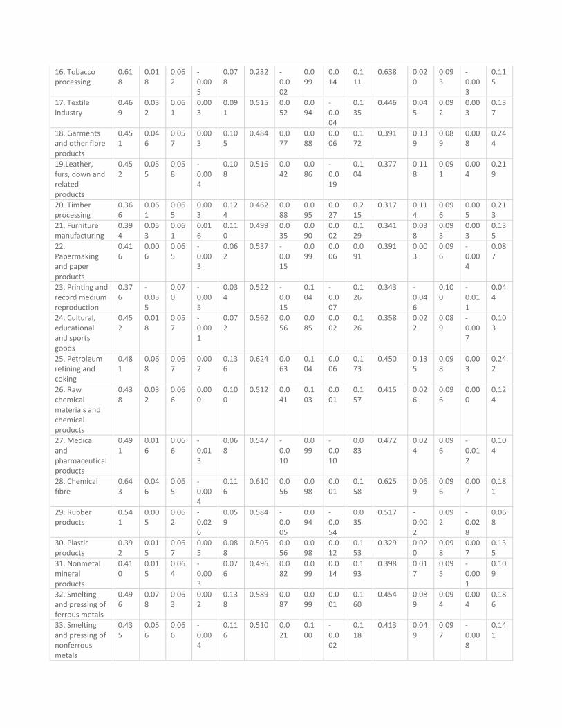
Average growth indices of TEC, TP, SEC and the MI for each industry are reported in Table 5. All industries in our sample exhibit productivity growth, shown by a positive change in the MI. We also note that the majority contributions to productivity growth come from TP and TEC. The contribution from SEC is much smaller, not surprising given our short time span. Across all firms in our sample, total factor productivity grows at an average rate of 9.8% each year, among which efficiency improves by 3.6% and TP is 6.4%, while there is no discernible change in scale efficiency. With regard to individual industries, smelting and pressing of ferrous metals realizes the highest productivity growth of 13.8%, owing to a 7.8% growth in efficiency, a 6.3 % increase in TP, and a 0.2% increase in SEC. On the other hand, printing and record medium reproduction experiences the lowest productivity growth rate of 3.4% among all industries in our sample. Although firms in printing and record medium reproduction achieve an annual average of 7% in TP, the average efficiency of firms in this industry actually decreases by 3.5%.

Table 5. Productivity growth decomposition: Malmquist index, 2002-2004 All

firms

Foreign firmsa

Domestic firmsb

Industry TE (level)

TEC TP SEC MI TE (level)

TEC TP SEC MI TE (level)

TEC TP SEC MI

13. Food processing

0.338

0.044

0.068

0.004

0.114

0.427 0.007

0.100

-0.002

0.108

0.304 0.063

0.099

0.004

0.163

14. Food production

0.398

0.026

0.065

0.006

0.094

0.501 0.053

0.094

-0.009

0.137

0.364 0.052

0.097

0.013

0.156

15. Beverage industry

0.411

-0.009

0.066

-0.008

0.050

0.549 0.021

0.098

-0.010

0.097

0.375 -0.007

0.097

-0.007

0.085

16. Tobacco processing

0.618

0.018

0.062

-0.005

0.078

0.232 -0.002

0.099

0.014

0.111

0.638 0.020

0.093

-0.003

0.115

17. Textile industry

0.469

0.032

0.061

0.003

0.091

0.515 0.052

0.094

-0.004

0.135

0.446 0.045

0.092

0.003

0.137

18. Garments and other fibre products

0.451

0.046

0.057

0.003

0.105

0.484 0.077

0.088

0.006

0.172

0.391 0.139

0.089

0.008

0.244

19.Leather, furs, down and related products

0.452

0.055

0.058

-0.004

0.108

0.516 0.042

0.086

-0.019

0.104

0.377 0.118

0.091

0.004

0.219

20. Timber processing

0.366

0.061

0.065

0.003

0.124

0.462 0.088

0.095

0.027

0.215

0.317 0.114

0.096

0.005

0.213

21. Furniture manufacturing

0.394

0.053

0.061

0.016

0.110

0.499 0.035

0.090

0.002

0.129

0.341 0.038

0.093

0.003

0.135

22. Papermaking and paper products

0.416

0.006

0.065

-0.003

0.062

0.537 -0.015

0.099

0.006

0.091

0.391 0.003

0.096

-0.004

0.087

23. Printing and record medium reproduction

0.376

-0.035

0.070

-0.005

0.034

0.522 -0.015

0.104

-0.007

0.126

0.343 -0.046

0.100

-0.011

0.044

24. Cultural, educational and sports goods

0.452

0.018

0.057

-0.001

0.072

0.562 0.056

0.085

0.002

0.126

0.358 0.022

0.089

-0.007

0.103

25. Petroleum refining and coking

0.481

0.068

0.067

0.002

0.136

0.624 0.063

0.104

0.006

0.173

0.450 0.135

0.098

0.003

0.242

26. Raw chemical materials and chemical products

0.438

0.032

0.066

0.000

0.100

0.512 0.041

0.103

0.001

0.157

0.415 0.026

0.096

0.000

0.124

27. Medical and pharmaceutical products

0.491

0.016

0.066

-0.013

0.068

0.547 -0.010

0.099

-0.010

0.083

0.472 0.024

0.096

-0.012

0.104

28. Chemical fibre

0.643

0.046

0.065

-0.004

0.116

0.610 0.056

0.098

0.001

0.158

0.625 0.069

0.096

0.007

0.181

29. Rubber products

0.541

0.005

0.062

-0.026

0.059

0.584 -0.005

0.094

-0.054

0.035

0.517 -0.002

0.092

-0.028

0.068

30. Plastic products

0.392

0.015

0.067

0.005

0.088

0.505 0.056

0.098

0.012

0.153

0.329 0.020

0.098

0.007

0.135

31. Nonmetal mineral products

0.410

0.015

0.064

-0.003

0.076

0.496 0.082

0.099

0.014

0.193

0.398 0.017

0.095

-0.001

0.109

32. Smelting and pressing of ferrous metals

0.496

0.078

0.063

0.002

0.138

0.589 0.087

0.099

0.001

0.160

0.454 0.089

0.094

0.004

0.186

33. Smelting and pressing of nonferrous metals

0.435

0.056

0.066

-0.004

0.116

0.510 0.021

0.100

-0.002

0.118

0.413 0.049

0.097

-0.008

0.141

34. Metal products

0.440

0.047

0.064

0.004

0.113

0.564 0.017

0.096

0.003

0.107

0.368 0.044

0.095

0.001

0.144

35. Ordinary machinery

0.424

0.048

0.063

0.003

0.115

0.571 0.082

0.097

0.010

0.193

0.383 0.048

0.094

0.004

0.129

36. Special purposes equipment

0.476

0.046

0.062

-0.001

0.107

0.487 0.081

0.098

0.008

0.176

0.459 0.043

0.092

-0.008

0.135

37. Transport equipment

0.510

0.032

0.062

-0.001

0.093

0.594 0.067

0.097

-0.002

0.161

0.478 0.037

0.092

0.004

0.145

39. Other electronic equipment

0.472

0.037

0.063

0.000

0.099

0.577 0.036

0.093

0.001

0.127

0.415 0.050

0.095

0.002

0.156

40. Electric equipment and machinery

0.645

0.049

0.061

-0.006

0.101

0.662 0.075

0.092

-0.012

0.153

0.559 0.062

0.093

0.011

0.130

41. Electronic and telecommunications

0.533

0.042

0.060

-0.020

0.070

0.631 0.076

0.089

0.004

0.131

0.417 0.052

0.094

-0.013

0.062

42. Instruments and meters

0.490

0.043

0.060

-0.009

0.095

0.492 0.147

0.089

0.024

0.280

0.451 -0.003

0.092

-0.032

0.167

43. Other manufacturingc

0.431

0.039

0.065

0.001

0.105

- - - - - 0.408 0.077

0.096

-0.006

Mean 0.452

0.036

0.064

0.000

0.098

0.564 0.041

0.064

0.000

0.104

0.423 0.035

0.064

-0.001

0.097

Standard deviation

0.240

0.268

0.032

0.103

0.297

0.218 0.242

0.033

0.113

0.279

0.237 0.274

0.032

0.101

0.301

No. of obs. 36359

23942

24716

23229

22528

7380 4865

5020

4710

4572

28979 19077

19696

18519

17956

aForeign firms represents firms with at least 25% of foreign capital; bDomestic firms represents firms with less than 25% of foreign capital. cNo firm in other manufacturing industry has at least 25% of foreign capital. Data come from World Bank Enterprise Survey, China 2005.

Table 6. Results with world bank enterprise survey, China 2012 Panel (a): Production function

FDI (10%) FDI (25%) Horiz., up- & down-stream FDI (25%)

VARIABLES Coefficient Std. err.

Coefficient Std. err.

Coefficient Std. err.

ln(K) -0.63106*** [0.136] -0.61752*** [0.136] -0.60381*** [0.135] ln(L) 1.03011*** [0.197] 0.72789*** [0.207] 0.73756*** [0.190] ln(K)^2 0.06889*** [0.010] 0.06870*** [0.010] 0.06692*** [0.010] ln(L)^2 0.02375 [0.026] 0.03741 [0.030] 0.02999 [0.028] ln(K) × ln(L) -0.03692 [0.028] -0.04149 [0.028] -0.03634 [0.028] Constant 14.14936*** [1.027] 15.17329*** [1.093] 15.02829*** [1.065] Industry dummies Yes Yes Yes Regional dummies Yes Yes Yes

Panel (b): Technical inefficiency

Size 0.185 [0.123] -0.10661* [0.060] -0.09477** [0.044] Age -0.0025 [0.004] -0.00396 [0.004] -0.00299 [0.003] Foreign -0.21034** [0.095] -0.32078** [0.140] -0.63451*** [0.223] FDI Hori 0.45449** [0.204] FDI Up 0.92013 [1.096] FDI Down -2.86719* [1.694] Constant -0.38513 [0.305] 0.77317** [0.351] 0.70608** [0.277] Mean technical efficiency (TE)

0.6994367 0.793049 0.7995556

Gamma 0.0000453 0.0002264 0.0005139 Log likelihood -1326.7516 -1325.804 -1303.425 Wald Chi2 2866.08 2788.5 2873.09 Observations 1,098 1,098 1,084

Standard errors in brackets. *** p<0.01, ** p<0.05, * p<0.1. Data come from the World Bank Enterprise Survey, China 2012 Table 7. Technical efficiency gap between domestic and foreign firms

Industry 2005a TE gap 2005 survey

Industry 2012b TE gap 2012 survey

Food processing 40.40% Food production 37.59% Food 33.72% Beverage industry 46.48% Textile industry 15.54% Textiles 29.99% Garments and other fibre products 23.74% Garments 26.68% Timber processing 45.86% Wood 12.75% Papermaking and paper products 37.54% Paper 28.66% Raw chemical materials and chemical products

23.36% Chemicals 26.37%

Rubber products 12.97% Plastic and Rubber 22.35%

Plastic products 53.58%

Nonmetal mineral products 24.74% Non Metallic mineral products

28.28%

Metal products 53.17% Fabricated metal products 24.28% Basic metals 28.46%

Ordinary machinery 49.17% Machinery and equipment 27.75% Special purposes equipment 6.26%

Transport equipment 24.25% Transport machines 25.38% Other electronic equipment 39.05% Electronics 26.17% Electronic and telecommunications 51.61%

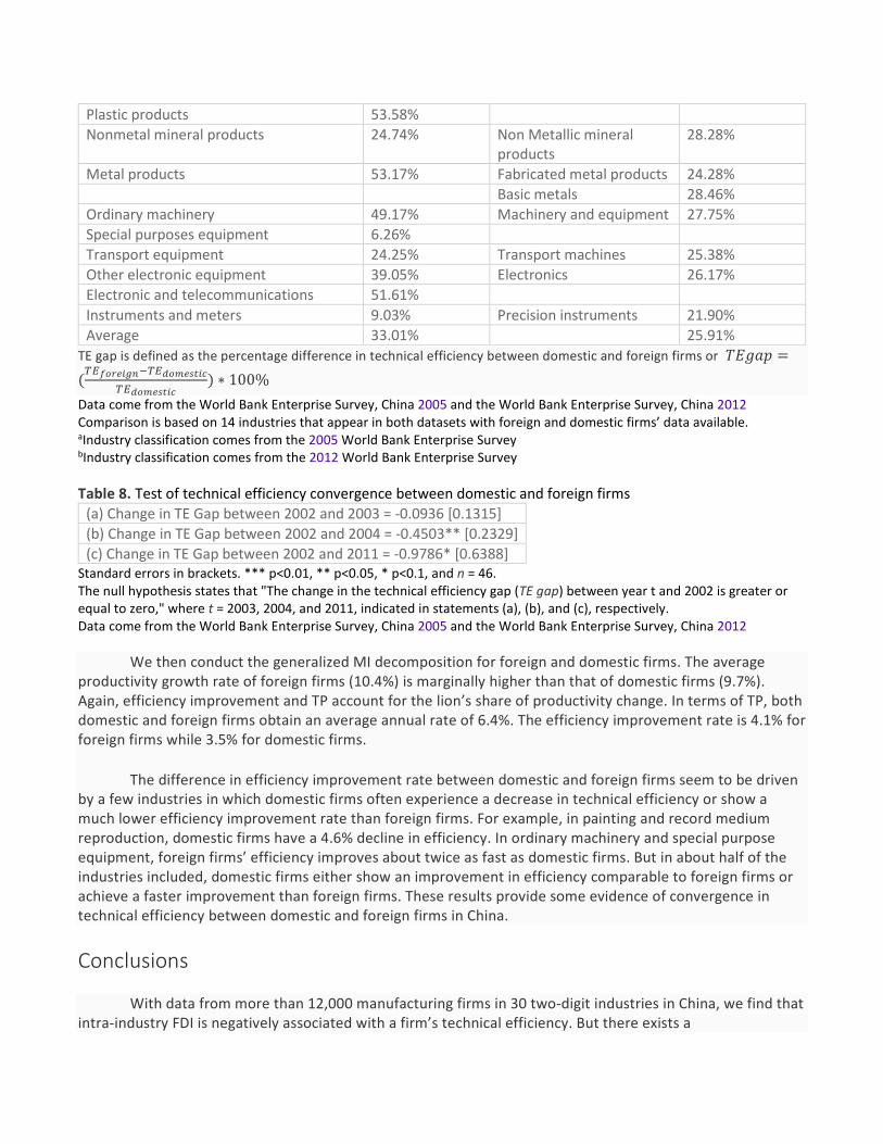
Instruments and meters 9.03% Precision instruments 21.90% Average 33.01% 25.91%

TE gap is defined as the percentage difference in technical efficiency between domestic and foreign firms or 𝑇𝑇𝐸𝐸𝐹𝐹𝑎𝑎𝑇𝑇 =(𝑇𝑇𝐸𝐸𝑓𝑓𝑓𝑓𝑓𝑓𝑓𝑓𝑖𝑖𝑓𝑓𝑓𝑓−𝑇𝑇𝐸𝐸𝑑𝑑𝑓𝑓𝑑𝑑𝑓𝑓𝑑𝑑𝑖𝑖𝑖𝑖𝑑𝑑

𝑇𝑇𝐸𝐸𝑑𝑑𝑓𝑓𝑑𝑑𝑓𝑓𝑑𝑑𝑖𝑖𝑖𝑖𝑑𝑑) ∗ 100%

Data come from the World Bank Enterprise Survey, China 2005 and the World Bank Enterprise Survey, China 2012 Comparison is based on 14 industries that appear in both datasets with foreign and domestic firms’ data available. aIndustry classification comes from the 2005 World Bank Enterprise Survey bIndustry classification comes from the 2012 World Bank Enterprise Survey Table 8. Test of technical efficiency convergence between domestic and foreign firms

(a) Change in TE Gap between 2002 and 2003 = -0.0936 [0.1315] (b) Change in TE Gap between 2002 and 2004 = -0.4503** [0.2329] (c) Change in TE Gap between 2002 and 2011 = -0.9786* [0.6388]

Standard errors in brackets. *** p<0.01, ** p<0.05, * p<0.1, and n = 46. The null hypothesis states that "The change in the technical efficiency gap (TE gap) between year t and 2002 is greater or equal to zero," where t = 2003, 2004, and 2011, indicated in statements (a), (b), and (c), respectively. Data come from the World Bank Enterprise Survey, China 2005 and the World Bank Enterprise Survey, China 2012

We then conduct the generalized MI decomposition for foreign and domestic firms. The average productivity growth rate of foreign firms (10.4%) is marginally higher than that of domestic firms (9.7%). Again, efficiency improvement and TP account for the lion’s share of productivity change. In terms of TP, both domestic and foreign firms obtain an average annual rate of 6.4%. The efficiency improvement rate is 4.1% for foreign firms while 3.5% for domestic firms.

The difference in efficiency improvement rate between domestic and foreign firms seem to be driven by a few industries in which domestic firms often experience a decrease in technical efficiency or show a much lower efficiency improvement rate than foreign firms. For example, in painting and record medium reproduction, domestic firms have a 4.6% decline in efficiency. In ordinary machinery and special purpose equipment, foreign firms’ efficiency improves about twice as fast as domestic firms. But in about half of the industries included, domestic firms either show an improvement in efficiency comparable to foreign firms or achieve a faster improvement than foreign firms. These results provide some evidence of convergence in technical efficiency between domestic and foreign firms in China.

Conclusions

With data from more than 12,000 manufacturing firms in 30 two-digit industries in China, we find that intra-industry FDI is negatively associated with a firm’s technical efficiency. But there exists a

complementarity between horizontal FDI and individual firm’s R&D. Our results also show that FDI in a firm’s downstream industries increases the firm’s technical efficiency while FDI in a firm’s upstream industries decreases the firm’s efficiency. A generalized Malmquist index decomposition also shows foreign firms on average achieve a higher productivity growth than domestic firms in China and the difference is mainly due to a faster technical efficiency improvement by foreign firms.

Our findings have important implications for policy makers. Positive effects of FDI on efficiency are clearly not automatic. As a result, simply attracting more FDI may not necessarily lead to a general productivity gain in the host economy. More importantly, since the effects of FDI can be different across industries, we do not recommend a “one-size-fits-all” investment promotion policy. Host governments should evaluate potential costs and benefits when inviting foreign investments and engage in “policy specialization” to improve their foreign spillovers conditions. It is also crucial to implement policies for strengthening the absorptive capacity of domestic firms. This can be done either through direct subsidies to firms that conduct R&D or through economy-wide policies promoting human capital formation. There is also a need for general policies to build modern infrastructure and increase the quality of institutions. In addition, policies that help domestic firms to upgrade their products may be warranted so that domestic firms are more likely to purchase intermediate inputs produced by foreign firms in upstream industries.

As in other studies, the present paper has its limitations. Because of data availability issues, we are unable to fully explore the dynamics of technical efficiency of domestic and foreign firms over time. A potential topic for future research that emerges from this study is to examine technical efficiency improvements, technical progress as well as changes in scale efficiencies if a sample covering a common set of industries over a longer time period is available (e.g. 2005-2012). Another interesting direction for future research could be to further study heterogeneity in firm efficiency across different industries. For example, our main results in Table 5 show substantial industry heterogeneity in terms of productivity growth and similarly, certain industry-level heterogeneity is noted in results in Appendix Table 7 with more recent data. In Appendix Table 7, seven of the 14 industries (based on the 2012 survey classification) in our sample exhibit significant decline in the efficiency gap between domestic and foreign firms. The seven industries are food, wood, paper, plastic and rubber, fabricated metal products, basic metals, and electronics. In five of the 14 industries, the efficiency gap between domestic and foreign firms seems to grow over time, which include textiles, garments, chemicals, non-metallic mineral products, and precision instruments. The other two industries, machinery and equipment and transport machines, do not exhibit a significant change in the efficiency gap. Findings of future research on the variations in the results across different industries can have significant policy implications as they provide better insights on industry-specific behaviors.

Footnotes 1.We note that Kathuria (2001) adopts a two-stage approach and estimates production and inefficiency

functions separately. The two-stage approach, compared to the one-stage approach we employ in our paper, may potentially produce biased estimated coefficients (Kumbhakar et al. 1991).

2. It is also called the World Bank Enterprise Survey. 3. The 2005 survey includes 30 manufacturing industries and the 2012 survey includes 20 manufacturing

industries. The comparison is done based on 14 manufacturing industries that have both domestic and foreign firms and are included in both datasets.

4. See Lovell (2003) for a detailed discussion of studies on the decomposition of Malmquist index.

Notes Acknowledgments

The authors would like to thank Brian Brush, Jim Granato and all participants at the Economics Seminar in September 2012 for their comments and suggestions. Wang gratefully acknowledges financial support from the Center for Global and Economic Studies and the summer Miles Research Grant at Marquette University, Milwaukee, WI.

Appendix

Table 6

Table 7

Table 8

References 1. Aigner, D. J., Lovell, C. A. K., & Schmitdt, P. (1977). Formulation and estimation of stochastic frontier production

function models. Journal of Econometrics, 6(1), 21–37. 2. Aitken, B. J., & Harrison, A. E. (1999). Do domestic firms benefit from direct foreign investment? Evidence from

Venezuela. American Economic Review, 89(3), 605–618. 3. Alfaro, L., Kalemli-Ozcan, S., & Sayek, S. (2009). FDI, productivity and financial development. The World

Economy, 32(1), 111–135. 4. Bai, C., Lu, J., & Tao, Z. (2009). How does privatization work in China? Journal of Comparative Economics, 37(3),

453–470. 5. Balsvik, R. (2011). Is labor mobility a channel for spillovers from multinationals? Evidence from Norwegian

manufacturing. The Review of Economics and Statistics, 93(1), 285–297. 6. Battese, G., & Coelli, T. (1995). A model for technical inefficiency effects in a stochastic frontier production

function for panel data. Empirical Economics, 20(2), 325–332. 7. Blalock, G., & Gertler, P. (2008). Welfare gains from foreign direct investment from technology transfer to local

suppliers. Journal of International Economics, 74(2), 402–421. 8. Blalock, G., & Gertler, P. (2009). How firm capabilities affect who benefits from foreign technology. Journal of

Development Economics, 90(2), 192–199. 9. Caves, R. (1974). Multinational firms, competition and productivity in host-country markets. Economica, 41(162),

176–193. 10. Charoenrat, T., & Harvie, C. (2014). The Efficiency of SMEs in Thai manufacturing: a stochastic frontier

analysis. Economic Modelling, 43, 372–393. 11. Charoenrat, T., Harvie, C., & Amornkitvikai, Y. (2013). Thai manufacturing small and medium sized enterprise

technical efficiency: evidence from firm-level industrial census data. Journal of Asian Economics, 27, 42–56. 12. China National Bureau of Statistics (2006). Input-Output table of China 2002. Beijing: China Statistics Press. 13. Crespo, N., & Fontoura, M. (2007). Determinant factors of FDI spillovers – what do we really know? World

Development, 35(3), 410–425. 14. Driffield, N. (2004). Regional policy and spillovers from FDI in the UK. Annals of Regional Science, 38(4), 579–594.

15. Dunning, J. H. (1977). Trade, location of economic activity and the MNE: a search for an eclectic approach. In B. Ohlin, P. O. Hesselborn, & P. M. Wijkman (Eds.), The international allocation of economic activity (pp. 395–418). London: Macmillan.

16. Glass, A. J., & Saggi, K. (2002). Multinational firms and technology transfer. The Scandinavian Journal of Economics, 104(4), 495–513.

17. Hanousek, J., Kocenda, E., & Masika, M. (2012). Firm efficiency: domestic owners, coalitions, and FDI. Economic Systems, 36(4), 471–486.

18. Javorcik, B. (2004). Does foreign direct investment increase the productivity of domestic firms? In search of spillovers through backward linkages. American Economic Review, 94(3), 605–627.

19. Javorcik, B. (2008). Can survey evidence shed light on spillovers from foreign direct investment? The World Bank Research Observer, 23(2), 139–159.

20. Kathuria, V. (2001). Foreign firms, technology transfer and knowledge spillovers to Indian manufacturing firms – a stochastic frontier analysis. Applied Economics, 33(5), 625–642.

21. Kumbhakar, S., Ghosh, S., & McGuckin, T. (1991). A generalized production frontier approach for estimating determinants of inefficiency in U.S. dairy farms. Journal of Business and Economic Statistics, 9(3), 279–286.

22. Lall, S. (1980). Vertical inter-firm linkages in LDCs: an empirical study. Oxford Bulletin of Economics and Statistics, 42(3), 203–226.

23. Levinsohn, J., & Petrin, A. (2003). Estimating production functions using inputs to control for unobservables. Review of Economic Studies, 70(2), 317–341.

24. Lovell, C. A. K. (2003). The decomposition of Malmquist productivity indexes. Journal of Productivity Analysis, 20(3), 437–458.

25. Malmquist, S. (1953). Index numbers and indifference curves. Trabajos de Estadística, 4(2), 209–242. 26. Merlevede, B., Schoors, K., & Spatareanu, M. (2014). FDI spillovers and time since foreign entry. World

Development, 56, 108–126. 27. Oczkowski, E., & Sharma, K. (2005). Determinants of efficiency in least developed countries: further evidence

from Nepalese manufacturing firms. Journal of Development Studies, 41(4), 617–630. 28. Olley, S., & Pakes, A. (1996). The dynamics of productivity in the telecommunications equipment

industry. Econometrica, 64(6), 1263–1298. 29. Rodríguez-Clare, A. (1996). Multinationals, linkages, and economic development. American Economic Review,

86(4), 852–873. 30. Suyanto, A., Salim, R. A., & Bloch, H. (2009). Does foreign direct investment lead to productivity spillovers? Firm

level evidence from Indonesia. World Development, 37(12), 1861–1876. 31. Suyanto, A., Salim, R. A., & Bloch, H. (2014). Which firms benefit from foreign direct investment? Empirical

evidence from Indonesia manufacturing. Journal of Asian Economics, 33, 16–29. 32. World Bank (2005). World Bank Enterprise Survey Data. China, 2005.Available

from http://www.enterprisesurveys.org/dataAccessed 18 August 2012 33. World Bank (2012). 2012 World Bank Enterprise Survey Data, China.Accessed 8 January 2016.Available

from http://www.enterprisesurveys.org/data 34. World Bank (2013). Doing Business 2013: smarter regulations for small and medium-size enterprises.

Washington: World Bank. 35. Yaşar, M., & Paul, M. C. J. (2009). Size and foreign ownership effects on productivity and efficiency: an analysis

of Turkish motor vehicle and parts plants. Review of Development Economics, 13(4), 576–591. 36. Zhang, Y., Li, Y., & Li, H. (2014). FDI spillovers over time in an emerging market: the roles of entry tenure and

barriers to imitation. Academy of Management Journal, 57(3), 698–722. 37. Zhao, S. (2013). Privatization, FDI inflow and economic growth: evidence from China's provinces, 1978-

2008. Applied Economics, 45(15), 2127–2139.