Embed Size (px)
Citation preview

Documento de Trabajo Nro. 230
Julio, 2018
ISSN 1853-0168
www.cedlas.econo.unlp.edu.ar
The Effects of Being Subject to the Colombian Apprenticeship Contract on Manufacturing Firm Performance
Carlos Ospino

The effects of being subject to the Colombian apprenticeship
contract on manufacturing firm performance.
Carlos Ospino∗†‡
Universidad de los Andes
February 14, 2018
Abstract
This paper evaluates the intent to treat local average treatment effects of the Colombianapprenticeship contract on manufacturing firm dynamics taking advantage of an exogenousvariation generated by the 2002 labor reform and the regulation design. This evaluation is ap-pealing because very little is known about the effects of apprenticeship policies on firm dynamicsin developing countries. Moreover, although this regulation has been in place for years it hasnot been evaluated. Results using a regression discontinuity design which compares small firmssubject to the regulation to those that are not, shows positive effects on output per worker (10log points), total factor productivity (3 log points) and the share of exported sales (2 percentagepoints). It also shows a negative effect on the average wage bill of directly hired workers (9 logpoints). These results suggest that small firms which became subject to the regulation adjustedtheir labor force more efficiently, thus increasing productivity but did not share these gains withworkers through higher wages.
Keywords: Apprenticeships, firm productivity, regression discontinuity design.JEL Classification: C21, D22, O47
1 Introduction
The use of apprenticeship contracts is widespread in Latin America1. These regulations frequentlylink the use of apprenticeship contracts to firm size, either by limiting the maximum number of ap-prentices, or even by imposing quotas based on the number of regular workers. As such, regulationson apprenticeship contracts frequently fall within the category of size-dependent policies.
The impact of size-dependent policies on the efficiency of an economy has received increasingattention in the growth literature. Guner et al. (2008) have studied the effect of such policies for
∗This paper incorporates comments by the CEDLAS’ Grant for Graduate Thesis competition 2015 to the secondchapter of my doctoral dissertation. I thank Marcela Eslava for her valuable mentorship during this project. Allerrors are my own.†I acknowledge funding for this research project from CEDLAS. I thank anonymous referees from CEDLAS for
their helpful comments and suggestions.‡I thank my dissertation committe for their valuable comments and suggestions. They are: Juan Esteban Carranza,
Pablo Lavado, Carlos Medina and Andres Zambrano.1 ILO’s CEINTERFOR reports the existence of regulation for many Latin American countries including: Ar-
gentina, Brazil, Chile, Colombia, Costa Rica, Ecuador, El Salvador, Honduras, Peru, Panama, and Uruguay.http://www.oitcinterfor.org/jovenes/contratos-aprendizaje
1
1 INTRODUCTION
the size distribution of firms, productivity and output. In the first chapter I showed that laborsubstitution as a response to the apprenticeship contract can affect the allocation and compositionof labor among firms (Ospino, 2016). Understanding the effects of the apprenticeship contract onfirm productivity, wages and capital accumulation is vital to designing policies that consider howfirms are affected, since most evaluations only consider the effects of policies on those that receivetraining.
In this paper I take advantage of the exogenous variation in the apprenticeship contract in Colombiawhich made small firms subject to this regulation. I exploit the regulation’s design to identify theeffects on small firm outcomes of the use of apprenticeship contracts. This regulation and therelevant features for the analysis are discussed in section 2. The paper is related to at least threedifferent branches of the economics literature. A set of studies focuses on the impact of size-dependent policies on firm outcomes. This literature is both theoretical and empirical and findsthat restrictions on the use of capital or labor which are conditional on firm size can have importanteffects on aggregate productivity. Such policies can explain the emergence of smaller firms whichshift the size distribution to the left (Guner et al., 2008; Braguinsky et al., 2011; Garicano et al.,2013).
In their model, Guner et al. (2008) find that restrictions on labor use have larger effects on output,firm size and productivity, than restrictions on capital use because there are general equilibriumeffects, where the most important are lower wages and the creation of smaller firms. The mech-anism is the following. Higher labor costs reduce total labor demand which lowers wages. Lowerwages make less productive firms profitable and induces the emergence of smaller firms. In thissense, Braguinsky et al. (2011) and Garicano et al. (2013) provide evidence on size-dependent la-bor regulation in Portugal and France respectively, which affects labor allocation and productivity.Braguinsky et al. (2011) argue that the level of employment protection in Portugal, which theyconsider among the highest in OECD countries, explains a size distribution of firms shifted to theleft with respect to countries with less restrictive regulations. Their argument is that employmentprotection regulation affects disproportionately larger firms than smaller ones, thus providing in-centives to reduce size. Finally, Garicano et al. (2013) argue that employment protection lawsthat affect firms with at least 50 workers in France, explain important dead-weight losses that canbe as high as 5% of GDP. The current paper contributes to this literature by providing empiricalevidence of how a size-dependent regulation in a developing country affects the allocation of laborand capital around the threshold where the regulation kicks in.
A second group of studies focuses on the impact of apprenticeship contracts and other forms oftraining on firm labor productivity. The main message from this literature is that evaluatingtraining policies by just focusing on the wages of trainees is insufficient to capture all the benefitsof training, since it ignores increases in labor productivity. It finds that labor productivity gainscan be twice as much as wages gains, but these gains differ across economic sectors (Dearden et al.,2006; Mohrenweiser and Zwick, 2009; Konings and Vanormelingen, 2010). Dearden et al. (2006)find that the impact of training on wages is half the impact on firm labor productivity (0.35 and0.60, respectively), thus providing evidence of the underestimation of the impacts of training whenusing wages alone. They also show that this result is driven by sectors with low wages, suggestingthat the monopsony power by firms in these sectors allows for the difference between wages andproductivity gains. Mohrenweiser and Zwick (2009) use matched employer-employee level data toestimate the impacts of training apprentices on productivity measures of German firms between1997 and 2002. The paper’s main contribution is testing whether all sectors face costs of increasingthe share of apprentices, something that was taken for granted in the literature; they do this by
2
1 INTRODUCTION
considering apprentices in different types of occupations: manufacturing, craft and construction,and commercial occupations, within firms. In particular, only in the manufacturing sector anincrease in the share of apprentices reduces net profits, but has no effect on labor productivity(measured as value-added per worker). Konings and Vanormelingen (2010) study how voluntaryjob training undertaken by Belgian firms affects firm productivity. They use a panel of firmsthat report detailed information about training expenditures, the intensity of training and theshare of trained workers. They find that the productivity premium for trained workers relativeto those that did not receive training is 23% while the wage premium is 12%. They concludethat in this context it is optimal for firms to provide training since productivity rises by a higherfactor than the rise in wages. This effect is known as wage compression (Acemoglu and Pischke,1999). While this literature has assessed the effect of voluntary training on workers and firms, inColombia apprenticeship contracts are mandatory. This type of regulation has not been assessedand constitutes a relevant contribution to the training literature.
Finally, the paper is related to the literature about the effects of labor regulation reforms on themanufacturing sector’s performance (Besley and Burgess, 2004; Eslava et al., 2004). Besley andBurgess (2004) exploit state level variation over time in amendments to the Industrial Dispute Act(IDA) of 1947, using data from 1958 to 1992 and find that pro-worker legislation in India had anegative effect on investment, employment, productivity and output of formal manufacturing firms.It also increased informal manufacturing activity. Eslava et al. (2004) studied the role of factorallocation and demand shocks in explaining changes in productivity after several reforms took placein Colombia in the early 1990’s. While their focus is not exclusively on labor reforms, they find thatafter the reforms in the 90’s the allocation of production towards more productive firms increasedtotal factor productivity. The current paper provides evidence of how a particular size-dependentregulation reform to a flexible form of contracting that took place in 2002 and has not yet beenevaluated affected manufacturing firms’ performance in an institutional context which is differentfrom India but that nonetheless shares some similarities. For example, Ospino (2016) shows thatthe change in the apprenticeship contract regulation is associated with an increase in the use ofoutsourced labor contracts in Colombia. Bertrand et al. (2015) show that the IDA, a size-dependentregulation, is associated with the increased use of contract labor from staffing companies by Indianfirms with more than 100 workers. Bertrand et al. (2015) find that the availability of a flexibleform of contracting allowed firms to invest in risky projects, increase total labor demand and copewith demand shocks in spite of the tight labor regulation they are subject to. Therefore, I will testwhether the observed labor outsourcing by Colombian small manufacturing firms as a response tothe apprenticeship contract is associated with capital investment decisions by firms.
The paper is structured as follows. The first section is this introduction. In section 2 I look at therelevant features of the regulation which are important for its evaluation. In section 3 I explainthe empirical approximation to evaluate the effects of this policy on firm performance. In section4 I discuss validity tests for the empirical approximation as well as the results of the econometricexercises. Finally section 5 ends with a discussion of the main findings and its implications forpublic policy. In the Appendix I provide additional results and robustness checks for the mainexercise.
3

2 REGULATORY FRAMEWORK
2 Regulatory framework
2.1 Regulation before 2003.
Law 188 of 1959 established the nature of the apprenticeship contract as a labor contract. Ap-prentices were employees of the firm and the labor code regulated this working relationship. Theirsalary could not be lower than 50% of the minimum wage and it had to increase as the appren-tice gained knowledge in her craft until it reached at least a full minimum wage. Decree 2838 of1960 established that employers with more than US$15,0002 in capital or more than 20 permanentworkers, had the obligation of hiring apprentices. The number of apprentices could not exceed 5%of firm personnel. Given that apprenticeships could only be hired for occupations defined by thelabor ministry based on recommendations by SENA (Colombia’s vocational and training institu-tion), only students of programs offered or recognized by SENA could be hired using apprenticeshipcontracts. The prevalent form of compliance with the regulation was modifying regular workerslabor contracts and providing time for training. This practice allowed employers to train theirworkforce at SENA’s nocturnal programs while these continued to work in their regular daily shift.Such an alternative allowed firms to comply with the regulation without affecting their labor forceor reducing production. Accordance 007 of 2000 established that the regulated quota would bedetermined using the number of skilled workers at the firm. The amendment defined skilled workeras those in the list occupations for which an apprenticeship contract could be signed. In practice 3
the apprenticeship quota was calculated using only the number of non-production regular workerswhich was known as the “administrative staff” at the firm.
2.2 Regulation after 2003.
Law 789 of 2002 was a major labor reform approved on December 27 of that year, which overhauledamong other things, the apprenticeship contract regulation. For example, article 30 changed thelegal nature of the apprenticeship contract from a regular labor contract to a special form of hiringwhich no longer implied an employer-employee relationship. The law limited the duration of eachcontract to a maximum of 2 years and stated that apprentices must receive a monetary stipend.Thus, starting in January of 2003 apprentices were no longer considered firm employees. Thissame article established that compensation will be as follows: 50% of a minimum wage during theclassroom training phase and 75% for the duration of the on-the-job training phase (100% of aminimum wage in the case university students4.).
Article 32 states that firms which hire at least 15 workers in any sector, except in construction,are obligated to hire apprentices for the occupations related to their economic activity. Article 33defined the regulated quota (RQ) as the minimum number of apprentices the firms must hire. Firmssubject to regulation must hire one apprentice for every 20 regular workers, and they must hire anadditional apprentice if the number of workers is a multiple of 10. Therefore firms between 15 and29 direct workers must hire one apprentice, firms between 30 and 49 workers must hire two, thosebetween 50 and 69 workers must have three apprentices and so on5. This same article states that ifthe apprenticeship contract were to end for any reason, the firm must replace the apprentice so that
2$100,000 Colombian pesos of the time, converted using the exchange rate provided by Colombia’s central bank.3I thank Lizeth Cortes for providing helpful information to understand the details of the previous regulation4University students can only be hired during the on-the-job training phase.5University students can only be hired to fulfill maximum 25% of the regulated quota.
4
2.2 Regulation after 2003. 2 REGULATORY FRAMEWORK
it always fulfills its RQ. Article 34 established an alternative way of complying with the RQ, whichis called “monetizing”. Under this option firms must pay a monthly fee to SENA. It is calculatedby multiplying 5% of their labor force size, excluding contractors and temporary workers, times theminimum wage. Article 35 established that the apprentice selection process will be carried out byfirms, but current or past employees can’t be hired under apprenticeship contracts. Apprenticeshipcontracts cannot be renewed once they’ve expired which implies that the same person can not bean apprentice more than once while obtaining a degree.
Apprenticeship contracts require firms to incur in other costs. In addition to an apprentice’scompensation, decree 933 (Signed in April) of 2003 established that firms must pay health andprofessional risk insurance for apprentices as if they earned a full minimum wage6. Given thatapprentices are not considered firm workers they are less costly than a minimum wage workerduring their productive phase. (Health costs amount to 8.5% while professional risk insurancerange from 0.348% to 8.7%, depending on the economic activity of the firm. See footnote 6). Atransitory paragraph in article 11 established that firms for which SENA had not established theRQ must do so themselves within 2 months of the decree’s publication. Therefore in practice, allfirms must have complied with the new regulation by June of 2003. Paragraph 1 allowed firmswith less than 15 regular workers to voluntarily have one apprentice even though these firms werein no obligation to do so. This option was initially only allowed for firms with less than 10 workersin Law 789 of 2002. Paragraph 2 of article 11 allows the firm to split the RQ among its differentplants according to its needs. Paragraph 3 allows firms to hire up to twice its RQ as long asthe firm does not reduce the number of regular employees used to calculate the quota. Article 14established the sanctions for not complying with the RQ in the amount of a full minimum wage forevery apprentice not hired or monetized, in addition to the amount due, including interest.
In short, the current regulation applies to a broader group of firms (especially small firms) thanbefore the reform took place since the quota is calculated based on the total number of regularworkers and not just non-production staff. In practical terms this modification more than doubledthe number of apprenticeship contracts between 2002 and 2003 from 33,000 to 72,000 per yearacross all economic sectors. However, it isn’t clear whether the regulation generated more costs thanbenefits for firms. While apprentices cost less during their productive phase than minimum wageworkers7, firms are required to pay for them even during their classroom training which becomes anet cost since classroom training can be as long as 75% of the apprenticeship’s duration.
Finally, firms subject to the regulation face other administrative costs which are not easy to quantify.For example, in July and December of every year firms must fill out forms informing SENA whetherthe number of workers hired during the past semester changed in a way which affects its RQ. Inthese forms firms must detail the number of workers in each occupation and the number of hoursthey work in a typical week. Once the form is filled out, firms must wait for the expedition of a legaldocument (Resolucion) which determines the new official quota. Further, selection and interviewof apprentices must be performed exclusively from the pool of candidates SENA lists in its websiteand the firm must incur in the affiliation costs of apprentices to social security and professional risksinsurance. These administrative costs are more likely to be important for firms around the firstthreshold of compliance with the apprenticeship contract since it implies incurring in the learning
6In Colombia the minimum wage is high and binding (Maloney and Mendez, 2004). Non-wage labor costs inColombia include severance payments, health and pension contributions, payroll taxes, two annual bonuses, vacationcompensation, and a transportation subsidy, all of which amounts to 66.6% for minimum wage workers (Mondragon-Velez et al., 2010).
7The apprenticeship contract regulation states that if the national unemployment rate falls below 10% apprenticesmust be paid a full minimum wage. The unemployment rate didn’t reach single digit levels in Colombia until 2010.
5
3 EMPIRICAL APPROXIMATION
costs of complying with a new regulation.
3 Empirical approximation
I now describe the data, the variables of interest and the econometric models to be used in estimatingthe impact of apprenticeship contracts on firm dynamics.
3.1 Data
The data for the main analysis comes from Annual Manufacturing Survey (EAM by its initials inSpanish) for the years 2001-20048. Rather than a survey as its name suggests, EAM is a censusof all formal manufacturing Colombian firms who hire at least 10 employees or generate an outputvalue of at least 35,000 USD. The number of manufacturing establishments range from 7.909 in 1995to 9.809 in 2011. It has very detailed information on output, sales, asset investments and interme-diate materials consumption, as well as labor demands broken down by different worker categories(e.g. temporary, permanent, men, women, skilled, managerial, production, non-production.) Thisinformation allows the estimation of production functions from which TFP is recovered. The dataare proprietary, administered by the National Statistical agency (DANE) and must be accessedon-site at DANE’s External Special Processing Room (SPEE for its initials in spanish).
3.2 Construction of outcome and control variables
All monetary variables are expressed in 2011 prices using DANE’s producer price index (IPP). TheIPP varies by industry class at the two digit ISIC code (CIIU Revision 3 AC).
Output.–It is measured as the wholesale value of all goods manufactured by the establishmentnet of indirect taxes.
Investment.–It is constructed as the net purchases of assets, excluding buildings and land.
Capital.–It is constructed using the iterative equation Kt = Kt−1 ∗ (1 − δ) + It. Where δ isthe depreciation rate (which was set to 5%) and It is asset investment by firms. The capitalmeasure also excludes buildings and land purchases or sales.
TFP.–Total factor productivity was estimated using the methods by De Loecker and Warzyn-ski (2012) and De Loecker (2013). These authors estimate a parametric Cobb-Douglas pro-duction function, f(k, l,m) = Akαlβmσ. Where k is capital, l is labor, and m is intermediatematerials. Total factor productivity follows an order 1 autoregressive process which also afunction of past exporting status9.
Skilled and Unskilled labor.–Skilled labor is defined as production professionals and techni-cians, while unskilled labor is defined as production laborers and operators. Both categoriesexclude non production workers and apprentices.
8I also constructed a longer longitudinal version of the dataset for the period 1995-2011 following the methodsproposed by Eslava and Melendez (2011). This latter dataset was used to test the validity of using a difference-in-difference approximation for the current analysis.
9A second method to estimate production function parameters used the parameters estimated by Eslava et al.(2004) for the period 1982-1998 to construct TFP.
6

3.3 Empirical strategy 3 EMPIRICAL APPROXIMATION
Wage bill.–Direct labor wage bill, includes wages of permanent and temporary workers di-rectly hired by the firm but excludes social security payments and benefits of these workers.Outsourced labor wage bill includes the payments of all production workers hired throughtemporary third party agencies.
Exports.–Two variables were used. The first variable indicates whether the firm is an exporteror not. Exporters are defined as any firm reporting positive amounts of the share of salesexported. A second variable measures the share of sales exported, in levels.
3.3 Empirical strategy
An empirical evaluation of the impact of the Colombian apprenticeship contract on firm outcomesis appealing for several reasons. The natural experiment generated by the reform allows the esti-mation of the causal effect of this regulation on measures of firm productivity such as total factorproductivity (TFP) and output per worker. Given that the empirical strategy to identify the pa-rameter of the production function from which TFP is recovered, rests on the assumption thatTFP evolves conditional on the exporting status of firms, it makes sense to explore whether theregulation also had an impact on the likelihood and the levels of exporting. It also allows to testwhether this regulation had an impact on the substitution of capital for labor and on firm invest-ment. While Ospino (2016) showed that the apprenticeship contract is associated with a reductionin total labor demand and the substitution between direct and outsourced labor, his model didnot incorporate capital and thus was not able to answer whether firms also substituted labor forcapital as a response to the policy. Finally, In addition to its negative effects on labor demand thisregulation could have affected worker wages. Therefore, an evaluation of its effects on the averageexpenditures on workers wages will be carried out.
The 2002 reform to the apprenticeship contract regulation affected firms in two ways: 1) Many smallfirms that were not subject to the apprenticeship contract regulation before 2002 were required to doso starting in 2003. 2) The regulation that is currently in place generates heterogeneity in the shareof apprentices that firms must hire. These shares change discontinuously at specific thresholds. Thispaper exploits the first feature and leaves the second one to be addressed in a subsequent paper10.Finally, the Colombian apprenticeship contract is similar to the ones used in other Latin Americancountries and apprenticeship contract regulations are a topic of regional interest. See Fazio et al.(2016) and http://blogs.iadb.org/trabajo/category/aprendices/ for a series of blogs on thesubject by The Inter-American Development Bank’ labor markets division. The key difference inColombia is its compulsory quota but it is, nevertheless, a useful regulation to understand howapprenticeship contracts can affect firm performance.
To evaluate the impact of being subject to the apprenticeship contract, an appealing methodologicalapproach is a Difference-in-Difference (DD) estimation because it exploits the fact that before theregulation changed some small firms were not subject to the regulation and in spite of the changethey are still not required to comply with it while other firms of similar size are. A deeper analysis ofthe data showed that the assumptions necessary for the DD estimation did not hold. In particularI found evidence of anticipation effects and trends did not follow a common-trend pattern11. Giventhese findings, to take advantage of the regulation threshold which separates near identical firms
10An earlier version of this paper estimated the impact of the share of apprentices on the outcomes of interest forseveral thresholds. For consistency with the first chapter in my doctoral dissertation which restricts the analysis tothe first threshold, the committee recommended that the other thresholds be studied in another paper.
11These exercises are available upon request.
7

3.3 Empirical strategy 3 EMPIRICAL APPROXIMATION
from having to comply with the apprenticeship contract, a regression discontinuity design waspreferred.
As discussed, the changes introduced by the 2002 reform can be exploited under a regression discon-tinuity design (RDD) to determine the effects of the apprenticeship contract on firm performancefor firms around the regulation threshold. This methodology relies on the similarities of the groupswhich are being compared. Firms locating before the threshold of compliance with this regulationwere likely to be similar to those which have to comply with it before the regulation changed. Noticefirst that the 2002 regulation changed the threshold level of compliance with the regulation from 20to 15 workers. And second, it changed the type of workers considered to determine the mandatoryquota from management staff to all directly hired workers. Therefore it’s very unlikely that firmshad incentives to change their directly hired labor demand at the threshold of compliance with theregulation before the reform was in effect. If firms had no incentives, and did not systematicallymodify the number of directly hired workers in 2002 to avoid compliance once the regulation wasin place, then treatment assignment into the regulation is “as good as” randomly assigned at thethreshold, and a RDD may be valid (Lee and Lemieux, 2009).
The validity of the RDD rests on the limited capacity of firms to perfectly control the assignmentvariable (the number of directly hired workers in the apprenticeship contract regulation), thereforesuch limited capacity is assumed. If it’s costly for firms in the short run to adjust the number ofdirectly hired workers, then these firms will not systematically fire workers in order to avoid beingsubject to the regulation. This could be due to a number of legal factors such as severance paymentsand contractual clauses, or economic factors such as positive demand shocks and technologicalrequirements in the production process. Figure 10 shows that in 2002 and 2003 a couple of newfirms hiring 15 direct workers appear in the data whereas in 2004 and 2005 no new firms are locatedexactly at this regulation threshold. This suggests that either firms did not anticipate the changesintroduced by the regulation at the threshold, or that they did not have incentives to avoid locatingat this threshold before the regulation was in full effect.
As a technical point, implementing the RDD to evaluate the apprenticeship contract must considerthe fact that the assignment variable, the number of directly hired workers at the firm, is discrete.In this case the limit of the expected value of the outcome of interest as we get arbitrarily close tothe threshold from either side does not exist and thus the only way to identify the model parameterof interest is through a parametric estimation (Lee and Card, 2008; Gelman and Imbens, 2014).I will follow the standard practice of clustering standard errors at each level of the assignmentvariable as suggested by Lee and Card (2008). Doing this takes into account the correlation offirms that have the same number of directly hired workers.
yij = β0 + β1Dij +m(Ndij , p)γp +Dij ×m(Ndij , p)αp + µij (1)
The model to be estimated is given by equation (1). The assignment variable Ndij is the numberof directly hired workers by each firm in 2002. It has been normalized so that it takes the valueof zero at the threshold cut-off value (15 directly hired workers). i indexes firms and j indexeseach discrete value of directly hired workers by firms, since standard errors are clustered at thislevel. The advantage of this normalization is interpreting β0 as the expected value of the outcomeat the threshold for firms not subject to the regulation. Dij = 1[Ndij ≥ 0] is an indicator variablethat identifies firms that hired between 15 and 24 directly hired workers in 2002. m(Ndij , p) is arow vector of a second degree polynomial of Ndij which is also defined in 200212. Dij ×m(Ndij , p)
12A second degree polynomial was used since it provides sufficient functional flexibility and Gelman and Imbens
8

4 RESULTS
allows polynomial slopes to differ for firms below and above the threshold of compliance.
β1 is the parameter of interest and captures the intent-to-treat (ITT) impact of the apprenticeshipcontract on firm outcome y since E[y|Ndij = 0, Dij = 1]−E[y|Ndij = 0, Dij = 0] ≡ β1. It estimatesthe ITT parameter since outcomes are measured in the year 2004, but treatment and assignmentvariable polynomials are defined using the observed direct labor demand in 2002. The analysistakes the year 2004 as the main estimation sample for two reasons: 1) Ospino (2016) shows thatfirm labor demand responded to the change in the apprenticeship contract regulation starting in2004. 2003 appeared to be a transition year since as discussed amendments to the regulation wereintroduced as far as June of that year. 2) In the year 2003 the number of apprentices hired wasnot reported in the data and these must be subtracted from total employment as apprentices arenot considered, by regulation, firm workers. Moreover, since having an apprentice implies beingsubject to the regulation, per worker variables would by construction be lower at the thresholdfor treated firms. For these reasons Dij determines whether firms should have been subject to theapprenticeship contract given their direct labor demand in 2002.
A possible concern to the identification strategy may be that firms not subject to the regulationcould voluntarily hire apprentices. As discussed in the regulation section, this exception was initiallyallowed for firms with 10 or less workers when the regulation changed in December of 2002, while themodifying decree changed this restriction in April of 2003. My preferred specification will comparefirms hiring between 11 and 19 workers, thus control firms were not allowed to hire apprenticeshipat the moment the assignment variable is measured.
4 Results
4.1 Assumptions and validity tests
In this section I carry out standard assumptions and validity test for RDDs to make sure theapproximation is appropriate for the current evaluation.
Changes in outcomes at the threshold
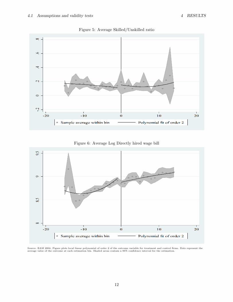
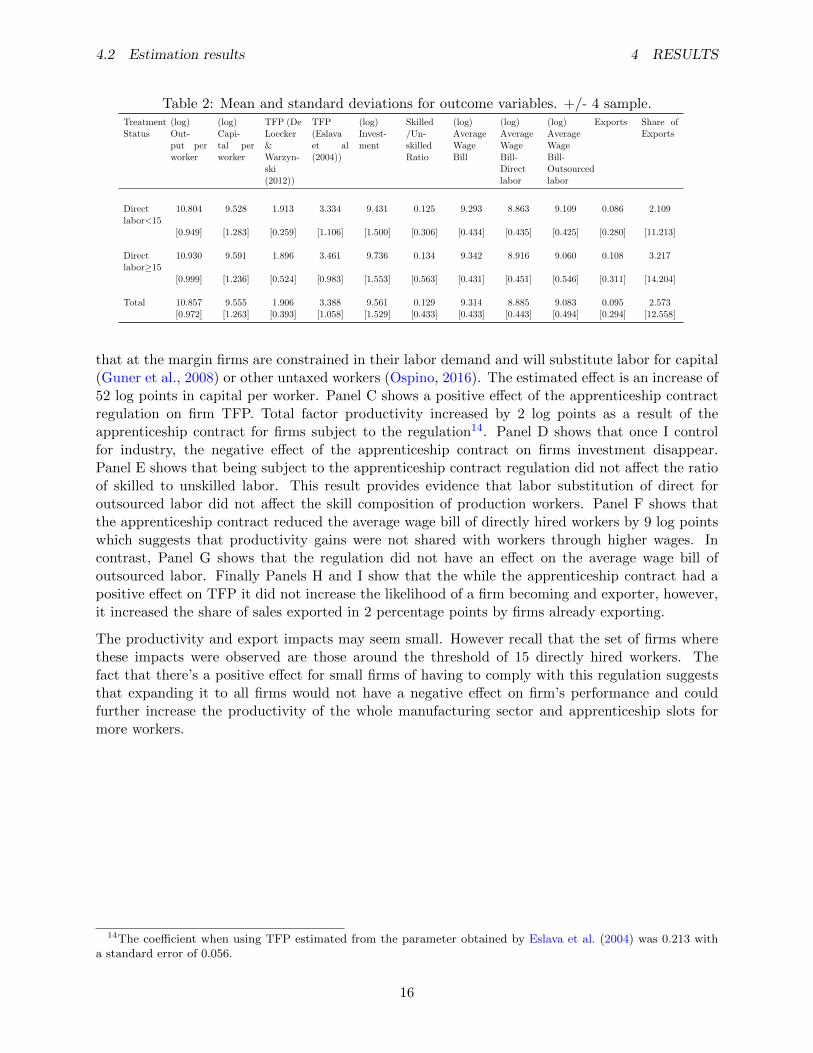
As Imbens and Lemieux (2008) suggest, graphical analysis is an integral part of the RDD. In thissection I show non parametric estimations of the outcome variable around the cutoff value whichshould provide insights for whether there are any effects of the regulation. Figures 1-9 show locallinear polynomial estimations that plot the relationship between outcomes in the year 2004 anddirect labor demand in 2002. These figures show that in all cases the slopes of the functions fittingthe data appear to be different for treatment and control firms which provides empirical support forestimating different slopes in equation (1). While point estimates appear to differ at the threshold,the 95% confidence intervals are so wide that one can not reject the null hypothesis of being equal.This second point suggests the inclusion of baseline covariates which may help reduce the samplevariability of the estimators (Lee and Lemieux, 2009).
(2014) warn against the use of higher order polynomials in RDD estimations.
9

4.1 Assumptions and validity tests 4 RESULTS
Figure 1: Average Log output per total number of workers
Figure 2: Average of Log capital per total number of workers
Source: EAM 2004. Figure plots local linear polynomial of order 2 of the outcome variable for treatment and control firms. Dots represent theaverage value of the outcome at each estimation bin. Shaded areas contain a 95% confidence interval for the estimation.
10

4.1 Assumptions and validity tests 4 RESULTS
Figure 3: Average Log Total Factor Productivity
Figure 4: Average Log Investment
Source: EAM 2004. Figure plots local linear polynomial of order 2 of the outcome variable for treatment and control firms. Dots represent theaverage value of the outcome at each estimation bin. Shaded areas contain a 95% confidence interval for the estimation.
11
4.1 Assumptions and validity tests 4 RESULTS
Figure 5: Average Skilled/Unskilled ratio
Figure 6: Average Log Directly hired wage bill
Source: EAM 2004. Figure plots local linear polynomial of order 2 of the outcome variable for treatment and control firms. Dots represent theaverage value of the outcome at each estimation bin. Shaded areas contain a 95% confidence interval for the estimation.
12

4.1 Assumptions and validity tests 4 RESULTS
Figure 7: Average Log Outsourced hired wage bill
Figure 8: Average Share of exporters
Source: EAM 2004. Figure plots local linear polynomial of order 2 of the outcome variable for treatment and control firms. Dots represent theaverage value of the outcome at each estimation bin. Shaded areas contain a 95% confidence interval for the estimation.
13

4.1 Assumptions and validity tests 4 RESULTS
Figure 9: Average Fraction of sales exported
Source: EAM 2004. Figure plots local linear polynomial of order 2 of the outcome variable for treatment and control firms. Dots represent theaverage value of the outcome at each estimation bin. Shaded areas contain a 95% confidence interval for the estimation.
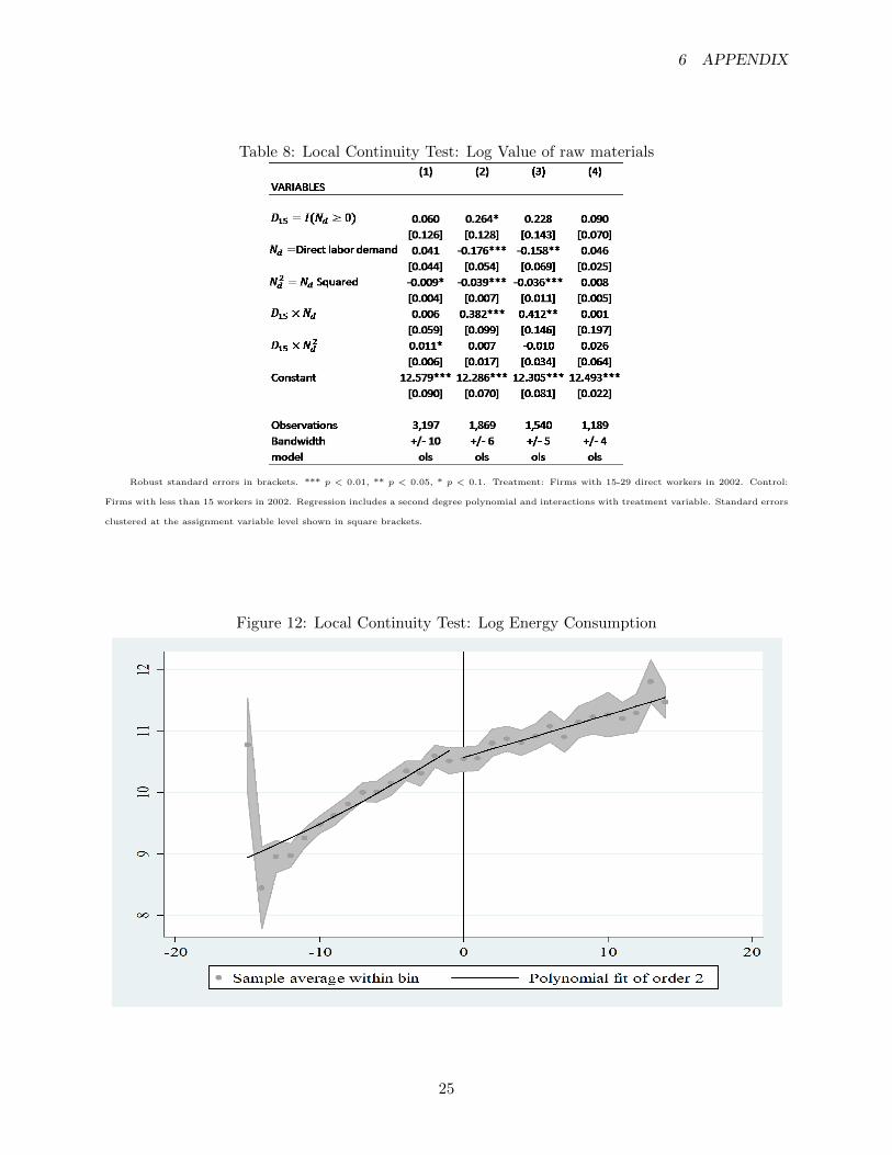
No manipulation and local continuityIn this section I show the results of the McCrary (2008) test of no manipulation. Local continuitytests of baseline covariates, namely intermediate inputs, energy consumption and firm age arepresented in the Appendix13.
Table 1 shows the results of performing a parametric version of McCrary (2008) test of no manip-ulation by estimating model (1) on a sample of the average values of each variable for each level ofNd ∈ (5, 24). The dependent variable is the Log number of firms at each level of direct labor de-mand. The parameter of interest is D15 which test whether the (log) number of firms is statisticallydifferent before and after the regulation threshold. The coefficient for the treatment variable is notsignificant for the +/−6 and +/−4 samples. This implies that the hypothesis that the assignmentvariable is continuous at the threshold of compliance with the regulation cannot be rejected andprovides evidence of no manipulation of the running variable. In section 6 of the Appendix I showthat the test is robust to using the number of firms at each level of direct labor demand, and thatthe result holds for the +/− 4 sample when D15 is defined using the observed direct labor demandin the year 2004. As a further robustness check, Table 4 shows that the no manipulation hypothesisis valid when the test is performed using the local polynomial density estimation introduced by therddensity command (Cattaneo et al., 2016). This particular test fails to reject the hypothesis thatthe distribution of direct labor do not differ at the threshold for the years 2002 and 2004. Thisconfirms our findings of the parametric McCrary (2008) test of no manipulation. However it rejectsthe null hypothesis of no manipulation for the year 2003. For the years 2002 and 2004 the testselected a data-driven bandwidths of [5.521, 5.527] and [5.978, 5.987] to the left and and right of
13Firm age showed a statistically significant difference of one year. Firms that in 2002 had a labor demand ofdirectly hired workers that would make them subject to the apprenticeship contract regulation had been establisheda year before firms that would not be subject to it.
14

4.2 Estimation results 4 RESULTS
Table 1: Parametric McCrary (2008) test of no manipulation
VARIABLES (1) (2) (3) (4)VARIABLES LN bin LN bin LN bin LN bin
D15 = I(Nd ≥ 0) -0.148*** -0.125 -0.252** -0.011[0.042] [0.088] [0.108] [0.046]
Nd=Normalized Directly hired demand -0.086*** -0.110 0.002 -0.263***[0.024] [0.073] [0.094] [0.051]
N2d = Nd Squared -0.003 -0.007 0.013 -0.044***
[0.002] [0.010] [0.015] [0.010]D15 ×Nd 0.096** 0.098 0.010 0.291***
[0.035] [0.074] [0.095] [0.053]D15 ×N2
d -0.003 0.008 -0.019 0.033**[0.004] [0.010] [0.015] [0.011]
Constant 5.009*** 4.985*** 5.104*** 4.859***[0.035] [0.087] [0.107] [0.046]
Observations 3,304 1,919 1,582 1,225Bandwidth +/- 10 +/- 6 +/- 5 +/- 4model ols ols ols ols
Robust standard errors in brackets. *** p < 0.01, ** p < 0.05, * p < 0.1. Treatment: Firms with 15-29 direct workers in 2002. Control:
Firms with less than 15 workers in 2002. Dependent variable is the Log number of firms at each size level. Regression includes a second degree
polynomial and interactions with treatment variable. Standard errors clustered at the assignment variable level.
the threshold for each year respectively.
4.2 Estimation results
Table 2 shows descriptive statistics of outcome variables for the main estimation sample.
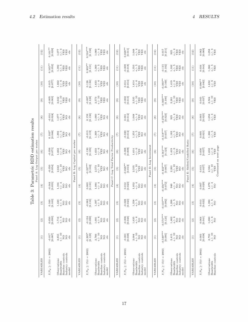
Table 3 shows the results of estimating equation (1) for the first threshold of compliance with theapprenticeship contract regulation. All columns include a second degree polynomial and interactionswith the treatment variable, which is measured in the year 2002. Columns (1)-(4) do not include anycontrols, columns (5)-(8) include baseline controls and columns (9)-(12) add industry indicators.Baseline controls, measured in 2002, are: The log value of intermediate materials used in production,the log value of electrical energy consumption in production and firm age, measured as the numberof years since it was created. Each group of regressions uses different samples around the thresholdof compliance with the apprenticeship contract. My preferred specification is column (12) whichcontrols for baseline covariates, industry of economic activity and uses the sample of firms between11 and 18 directly hired workers in 2002 (the +/−4 sample). Recall that the estimated coefficientsmust be interpreted as intent-to-treat effects.
Results in Panel A, show that the apprenticeship contract had a positive effect on output perworker. It increased labor productivity by 10 log points. The increase in output per worker isconsistent with the fact that firms subject to the regulation reduced their total number of workers(Ospino, 2016). Panel B shows evidence of substitution of labor for capital at the margin, which isconsistent with the findings of theoretical size-dependent distortion models. These models predict
15
4.2 Estimation results 4 RESULTS
Table 2: Mean and standard deviations for outcome variables. +/- 4 sample.TreatmentStatus
(log)Out-put perworker
(log)Capi-tal perworker
TFP (DeLoecker&Warzyn-ski(2012))
TFP(Eslavaet al(2004))
(log)Invest-ment
Skilled/Un-skilledRatio
(log)AverageWageBill
(log)AverageWageBill-Directlabor
(log)AverageWageBill-Outsourcedlabor
Exports Share ofExports
Directlabor<15
10.804 9.528 1.913 3.334 9.431 0.125 9.293 8.863 9.109 0.086 2.109
[0.949] [1.283] [0.259] [1.106] [1.500] [0.306] [0.434] [0.435] [0.425] [0.280] [11.213]
Directlabor≥15
10.930 9.591 1.896 3.461 9.736 0.134 9.342 8.916 9.060 0.108 3.217
[0.999] [1.236] [0.524] [0.983] [1.553] [0.563] [0.431] [0.451] [0.546] [0.311] [14.204]
Total 10.857 9.555 1.906 3.388 9.561 0.129 9.314 8.885 9.083 0.095 2.573[0.972] [1.263] [0.393] [1.058] [1.529] [0.433] [0.433] [0.443] [0.494] [0.294] [12.558]
that at the margin firms are constrained in their labor demand and will substitute labor for capital(Guner et al., 2008) or other untaxed workers (Ospino, 2016). The estimated effect is an increase of52 log points in capital per worker. Panel C shows a positive effect of the apprenticeship contractregulation on firm TFP. Total factor productivity increased by 2 log points as a result of theapprenticeship contract for firms subject to the regulation14. Panel D shows that once I controlfor industry, the negative effect of the apprenticeship contract on firms investment disappear.Panel E shows that being subject to the apprenticeship contract regulation did not affect the ratioof skilled to unskilled labor. This result provides evidence that labor substitution of direct foroutsourced labor did not affect the skill composition of production workers. Panel F shows thatthe apprenticeship contract reduced the average wage bill of directly hired workers by 9 log pointswhich suggests that productivity gains were not shared with workers through higher wages. Incontrast, Panel G shows that the regulation did not have an effect on the average wage bill ofoutsourced labor. Finally Panels H and I show that the while the apprenticeship contract had apositive effect on TFP it did not increase the likelihood of a firm becoming and exporter, however,it increased the share of sales exported in 2 percentage points by firms already exporting.
The productivity and export impacts may seem small. However recall that the set of firms wherethese impacts were observed are those around the threshold of 15 directly hired workers. Thefact that there’s a positive effect for small firms of having to comply with this regulation suggeststhat expanding it to all firms would not have a negative effect on firm’s performance and couldfurther increase the productivity of the whole manufacturing sector and apprenticeship slots formore workers.
14The coefficient when using TFP estimated from the parameter obtained by Eslava et al. (2004) was 0.213 witha standard error of 0.056.
16
4.2 Estimation results 4 RESULTS
Tab
le3:
Par
amet
ric
RD
Des
tim
atio
nre
sult
sP
anel
A:
Log
Outp
ut
per
work
er
VA
RIA
BL
ES
(1)
(2)
(3)
(4)
(5)
(6)
(7)
(8)
(9)
(10)
(11)
(12)
I(N
d≥
15|t
=2002)
-0.0
17
0.0
50
0.1
60
-0.0
44
-0.0
50
-0.0
56
0.1
03*
-0.0
14
-0.0
05
0.0
15
0.1
65**
0.1
01**
[0.0
87]
[0.0
93]
[0.1
03]
[0.0
55]
[0.0
54]
[0.0
71]
[0.0
46]
[0.0
24]
[0.0
63]
[0.0
77]
[0.0
52]
[0.0
29]
Obse
rvati
ons
2,8
55
1,7
16
1,4
23
1,1
04
2,6
42
1,6
62
1,3
92
1,0
77
2,6
42
1,6
62
1,3
92
1,0
77
Bandw
idth
+/-
10
+/-
6+
/-
5+
/-
4+
/-
10
+/-
6+
/-
5+
/-
4+
/-
10
+/-
6+
/-
5+
/-
4B
ase
line
contr
ols
NO
NO
NO
NO
YE
SY
ES
YE
SY
ES
YE
SY
ES
YE
SY
ES
Indust
rycontr
ols
NO
NO
NO
NO
NO
NO
NO
NO
YE
SY
ES
YE
SY
ES
model
ols
ols
ols
ols
ols
ols
ols
ols
ols
ols
ols
ols
Panel
B:
Log
Capit
al
per
work
er
VA
RIA
BL
ES
(1)
(2)
(3)
(4)
(5)
(6)
(7)
(8)
(9)
(10)
(11)
(12)
I(N
d≥
15|t
=2002)
-0.2
65*
-0.1
24
-0.0
62
0.0
63
-0.2
27**
-0.1
30
-0.0
13
0.1
59
-0.0
97
0.1
28
0.3
03**
0.5
16***
[0.1
29]
[0.0
99]
[0.1
16]
[0.1
31]
[0.1
02]
[0.1
05]
[0.1
19]
[0.1
36]
[0.1
28]
[0.1
30]
[0.1
31]
[0.1
38]
Obse
rvati
ons
2,7
66
1,6
81
1,3
97
1,0
84
2,5
73
1,6
33
1,3
69
1,0
60
2,5
73
1,6
33
1,3
69
1,0
60
Bandw
idth
+/-
10
+/-
6+
/-
5+
/-
4+
/-
10
+/-
6+
/-
5+
/-
4+
/-
10
+/-
6+
/-
5+
/-
4B
ase
line
contr
ols
NO
NO
NO
NO
YE
SY
ES
YE
SY
ES
YE
SY
ES
YE
SY
ES
Indust
rycontr
ols
NO
NO
NO
NO
NO
NO
NO
NO
YE
SY
ES
YE
SY
ES
model
ols
ols
ols
ols
ols
ols
ols
ols
ols
ols
ols
ols
Panel
C:
Log
Tota
lFacto
rP
roducti
vit
y
VA
RIA
BL
ES
(1)
(2)
(3)
(4)
(5)
(6)
(7)
(8)
(9)
(10)
(11)
(12)
I(N
d≥
15|t
=2002)
-0.0
01
-0.0
06
-0.0
28
0.0
12
-0.0
28**
-0.0
08
-0.0
20
0.0
01
-0.0
02
0.0
14
-0.0
09
0.0
28**
[0.0
38]
[0.0
46]
[0.0
43]
[0.0
23]
[0.0
13]
[0.0
09]
[0.0
12]
[0.0
12]
[0.0
13]
[0.0
14]
[0.0
18]
[0.0
11]
Obse
rvati
ons
2,6
84
1,6
35
1,3
58
1,0
52
2,5
35
1,6
14
1,3
53
1,0
48
2,5
35
1,6
14
1,3
53
1,0
48
Bandw
idth
+/-
10
+/-
6+
/-
5+
/-
4+
/-
10
+/-
6+
/-
5+
/-
4+
/-
10
+/-
6+
/-
5+
/-
4B
ase
line
contr
ols
NO
NO
NO
NO
YE
SY
ES
YE
SY
ES
YE
SY
ES
YE
SY
ES
Indust
rycontr
ols
NO
NO
NO
NO
NO
NO
NO
NO
YE
SY
ES
YE
SY
ES
model
ols
ols
ols
ols
ols
ols
ols
ols
ols
ols
ols
ols
Panel
D:
Log
Invest
ment
VA
RIA
BL
ES
(1)
(2)
(3)
(4)
(5)
(6)
(7)
(8)
(9)
(10)
(11)
(12)
I(N
d≥
15|t
=2002)
-0.5
49***
-0.5
74***
-0.4
10***
-0.4
56***
-0.4
32***
-0.5
61***
-0.3
18***
-0.2
76***
-0.3
69***
-0.3
93**
-0.1
15
0.0
17
[0.0
95]
[0.1
23]
[0.0
92]
[0.0
72]
[0.0
67]
[0.1
23]
[0.0
37]
[0.0
23]
[0.1
00]
[0.1
60]
[0.1
02]
[0.2
11]
Obse
rvati
ons
2,4
15
1,4
62
1,2
06
946
2,2
61
1,4
19
1,1
82
925
2,2
61
1,4
19
1,1
82
925
Bandw
idth
+/-
10
+/-
6+
/-
5+
/-
4+
/-
10
+/-
6+
/-
5+
/-
4+
/-
10
+/-
6+
/-
5+
/-
4B
ase
line
contr
ols
NO
NO
NO
NO
YE
SY
ES
YE
SY
ES
YE
SY
ES
YE
SY
ES
Indust
rycontr
ols
NO
NO
NO
NO
NO
NO
NO
NO
YE
SY
ES
YE
SY
ES
model
ols
ols
ols
ols
ols
ols
ols
ols
ols
ols
ols
ols
Panel
E:
Skille
d/U
nsk
ille
dR
ati
o
VA
RIA
BL
ES
(1)
(2)
(3)
(4)
(5)
(6)
(7)
(8)
(9)
(10)
(11)
(12)
I(N
d≥
15|t
=2002)
0.0
03
0.0
64
0.0
13
0.0
07
0.0
13
0.0
56
0.0
05
0.0
03
0.0
45
0.0
96**
0.0
34
0.0
62
[0.0
38]
[0.0
41]
[0.0
22]
[0.0
29]
[0.0
37]
[0.0
37]
[0.0
21]
[0.0
25]
[0.0
37]
[0.0
42]
[0.0
44]
[0.0
69]
Obse
rvati
ons
2,7
93
1,6
80
1,3
90
1,0
78
2,5
84
1,6
32
1,3
66
1,0
58
2,5
84
1,6
32
1,3
66
1,0
58
Bandw
idth
+/-
10
+/-
6+
/-
5+
/-
4+
/-
10
+/-
6+
/-
5+
/-
4+
/-
10
+/-
6+
/-
5+
/-
4B
ase
line
contr
ols
NO
NO
NO
NO
YE
SY
ES
YE
SY
ES
YE
SY
ES
YE
SY
ES
Conti
nued
on
next
page
17

4.2 Estimation results 4 RESULTS
–conti
nued
from
pre
vio
us
page
Indust
rycontr
ols
NO
NO
NO
NO
NO
NO
NO
NO
YE
SY
ES
YE
SY
ES
model
ols
ols
ols
ols
ols
ols
ols
ols
ols
ols
ols
ols
Panel
F:
Log
Avera
ge
wage
bill-
Dir
ect
lab
or
VA
RIA
BL
ES
(1)
(2)
(3)
(4)
(5)
(6)
(7)
(8)
(9)
(10)
(11)
(12)
I(N
d≥
15|t
=2002)
-0.0
84***
-0.1
32**
-0.0
95*
-0.1
78***
-0.0
98***
-0.1
44***
-0.1
07**
-0.1
83***
-0.0
57*
-0.0
78*
-0.0
15
-0.0
92**
[0.0
27]
[0.0
44]
[0.0
46]
[0.0
27]
[0.0
28]
[0.0
32]
[0.0
35]
[0.0
04]
[0.0
28]
[0.0
39]
[0.0
41]
[0.0
34]
Obse
rvati
ons
2,8
10
1,6
91
1,4
01
1,0
91
2,6
02
1,6
38
1,3
71
1,0
65
2,6
02
1,6
38
1,3
71
1,0
65
Bandw
idth
+/-
10
+/-
6+
/-
5+
/-
4+
/-
10
+/-
6+
/-
5+
/-
4+
/-
10
+/-
6+
/-
5+
/-
4B
ase
line
contr
ols
NO
NO
NO
NO
YE
SY
ES
YE
SY
ES
YE
SY
ES
YE
SY
ES
Indust
rycontr
ols
NO
NO
NO
NO
NO
NO
NO
NO
YE
SY
ES
YE
SY
ES
model
ols
ols
ols
ols
ols
ols
ols
ols
ols
ols
ols
ols
Panel
G:
Log
Avera
ge
Wage
bill-
Outs
ourc
ed
lab
or
VA
RIA
BL
ES
(1)
(2)
(3)
(4)
(5)
(6)
(7)
(8)
(9)
(10)
(11)
(12)
I(N
d≥
15|t
=2002)
-0.2
62***
-0.2
46**
-0.2
61***
-0.2
69***
-0.2
80***
-0.3
10**
-0.2
28***
-0.2
73***
-0.2
96*
-0.1
61
-0.1
24
-0.1
21
[0.0
54]
[0.0
87]
[0.0
44]
[0.0
55]
[0.0
68]
[0.1
00]
[0.0
65]
[0.0
67]
[0.1
42]
[0.2
39]
[0.2
48]
[0.3
26]
Obse
rvati
ons
379
245
204
154
364
236
196
148
364
236
196
148
Bandw
idth
+/-
10
+/-
6+
/-
5+
/-
4+
/-
10
+/-
6+
/-
5+
/-
4+
/-
10
+/-
6+
/-
5+
/-
4B
ase
line
contr
ols
NO
NO
NO
NO
YE
SY
ES
YE
SY
ES
YE
SY
ES
YE
SY
ES
Indust
rycontr
ols
NO
NO
NO
NO
NO
NO
NO
NO
YE
SY
ES
YE
SY
ES
model
ols
ols
ols
ols
ols
ols
ols
ols
ols
ols
ols
ols
Panel
H:
Exp
ort
er
VA
RIA
BL
ES
(1)
(2)
(3)
(4)
(5)
(6)
(7)
(8)
(9)
(10)
(11)
(12)
I(N
d≥
15|t
=2002)
-0.0
60**
-0.0
44
-0.0
03
0.0
09
-0.0
63**
-0.0
52*
-0.0
12
-0.0
01
-0.0
89***
-0.0
71**
-0.0
46**
-0.0
38
[0.0
25]
[0.0
27]
[0.0
15]
[0.0
19]
[0.0
24]
[0.0
24]
[0.0
10]
[0.0
14]
[0.0
31]
[0.0
30]
[0.0
19]
[0.0
22]
Obse
rvati
ons
2,8
62
1,7
15
1,4
21
1,1
03
2,6
38
1,6
58
1,3
89
1,0
75
2,6
38
1,6
58
1,3
89
1,0
75
Bandw
idth
+/-
10
+/-
6+
/-
5+
/-
4+
/-
10
+/-
6+
/-
5+
/-
4+
/-
10
+/-
6+
/-
5+
/-
4B
ase
line
contr
ols
NO
NO
NO
NO
YE
SY
ES
YE
SY
ES
YE
SY
ES
YE
SY
ES
Indust
rycontr
ols
NO
NO
NO
NO
NO
NO
NO
NO
YE
SY
ES
YE
SY
ES
model
ols
ols
ols
ols
ols
ols
ols
ols
ols
ols
ols
ols
Panel
I:Share
of
exp
ort
s
VA
RIA
BL
ES
(1)
(2)
(3)
(4)
(5)
(6)
(7)
(8)
(9)
(10)
(11)
(12)
I(N
d≥
15|t
=2002)
0.0
65
1.4
20
3.9
18***
5.6
91***
0.0
79
0.9
91
3.3
98***
5.1
37***
-1.2
64
-0.6
53
1.1
32
1.9
84**
[1.1
97]
[1.3
64]
[0.9
70]
[1.0
74]
[1.1
65]
[1.3
19]
[0.7
69]
[0.5
58]
[1.2
93]
[1.4
68]
[0.9
01]
[0.7
45]
Obse
rvati
ons
2,8
62
1,7
15
1,4
21
1,1
03
2,6
38
1,6
58
1,3
89
1,0
75
2,6
38
1,6
58
1,3
89
1,0
75
Bandw
idth
+/-
10
+/-
6+
/-
5+
/-
4+
/-
10
+/-
6+
/-
5+
/-
4+
/-
10
+/-
6+
/-
5+
/-
4B
ase
line
contr
ols
NO
NO
NO
NO
YE
SY
ES
YE
SY
ES
YE
SY
ES
YE
SY
ES
Indust
rycontr
ols
NO
NO
NO
NO
NO
NO
NO
NO
YE
SY
ES
YE
SY
ES
model
ols
ols
ols
ols
ols
ols
ols
ols
ols
ols
ols
ols
Sta
ndard
err
ors
clu
stere
dat
the
ass
ignm
ent
vari
able
level
show
nin
bra
ckets
.***
p<
0.0
1,
**
p<
0.0
5,
*p<
0.1
.T
reatm
ent:
Fir
ms
wit
h15-2
9dir
ect
work
ers
in2002.
Contr
ol:
Fir
ms
wit
hle
ssth
an
15
work
ers
in2002.
Regre
ssio
nin
clu
des
ase
cond
degre
ep
oly
nom
ial
and
inte
racti
ons
wit
htr
eatm
ent
vari
able
.
18

5 DISCUSSION
As a robustness check, in the Appendix, I show that most outcome variables do not show significanteffects in the year 2002, for different bandwidth samples. The two exceptions are, the capital perworker ratio and firm investment. These two variables showed positive coefficients of 57.4 and39.5 log points respectively, which suggests firms capital accumulation decisions might have beenaffected by other policies or that firms reacted in expectation to the regulation substituting capitalfor labor. For the other variables, the lack of anticipation effects provide further assurance that theresults found appear to be the effect of the policy and not of firms decisions before the regulationwas introduced. I also carried out the analysis using the sample for the year 2003. As discussed,given that labor substitution as a result of the policy did not take place until 2004 (Ospino, 2016),I did not expect to find significant effects. Section ?? in Appendix shows statistically significanteffects for capital per worker (72.6 log points), investment (49.6 log points), the skilled/unskilledratio (12.1 log points) and the share of exports (3.9 percentage points).
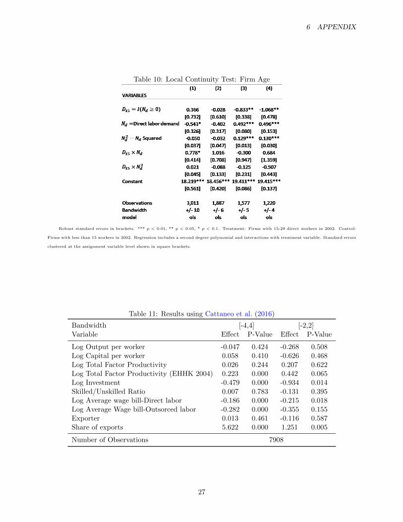
Finally, I estimated the effects following Cattaneo et al. (2016) using the rdrandinf package. Theseresults can be found in Table 11 where I show estimations for a second degree polynomial forthe same bandwidth as the main estimation (+4/-4) and the optimal selected bandwidth by thepackage (+2/-2). These results are consistent but of a higher magnitude for the average wage billof direct workers and the share of exports. Exporting status and the share of skilled and unskilledworkers are not significant as in the main results. However, output per worker and total factorproductivity which show positive and statistically significant effects in the main results are notstatistically significant in this estimation15. Another difference is that investment had a positiveeffect in the main results while in this estimation the effect is negative and statistically significant.Despite the differences my preferred results are the ones in Table 3. One reason is that I’m ableto control for industry fixed effects and still obtain results that speak about the manufacturingsector as a whole. Second, in Tables 14-17 in the Appendix I provide evidence about the presenceof heterogeneous effects by industry for the outcomes I can be confident about obtaining causaleffects following Cattaneo et al. (2016). These results provide support for the empirical strategywhere I control for industry fixed effects.
5 Discussion
In this paper I have used parametric regression discontinuity design (RDD) methods to evaluate theimpact of the apprenticeship contract on Colombian small firm dynamics. Firms showed statisticalsignificant differences at the moment when the regulation changed and most outcome variables donot follow a common trend before the regulation was reformed. Therefore, a difference-in-differenceapproximation which at first seemed appealing could not be used for this evaluation. Nevertheless,the assumptions for implementing a regression discontinuity design held, and therefore I proceededto carry out the evaluation using an intent-to-treat regression discontinuity design.
Results showed positive effects on output per worker, total factor productivity, and the share ofexports; it showed negative effects on the direct labor average wage bill. The increase in productivitymeasured by output per worker and total factor productivity suggests that the policy could havebenefited firms by increasing the skill component of their labor force. The increase in sales exportedpoints in the same direction. The absence of effects on the skill composition of labor suggests laborproductivity did not increase by firing unskilled labor. However, the negative effect on the average
15TFP calculated using the coefficients from Eslava et al. (2004) showed statistically significant effects of a similarmagnitude that when I used the parametric estimator in Equation 1.
19

BIBLIOGRAPHY BIBLIOGRAPHY
wage bill of directly hired workers and the absence of effects on the average wage bill of outsourcedworkers suggests that such productivity gains were not shared by firm workers through higherwages.
The policy implication of this paper is that having small firms being subject to the apprenticeshipcontract regulation had on average a positive effect on productivity for this group of firms whichreflected in higher output per worker and a higher share of exports. From the worker’s perspectivethe effect is a negative one since firm’s wage bill per directly hired worker decreased approximatelyby 9%. This result suggests that workers which determine whether firms are subject to the ap-prenticeship contract regulation or new hires could be the ones bearing the cost of the regulationdesign. A rigorous evaluation of this regulation for apprentices and regular workers employmentstatus and wages is a pending subject in Colombia to have a thorough assessment of the costs andbenefits of the apprenticeship contract regulation from the worker’s perspective.
Bibliography
Acemoglu, D. and J.-S. Pischke (1999). Beyond becker: Training in imperfect labour markets. TheEconomic Journal 109 (453), 112–142.
Bertrand, M., C. Hsieh, and N. Tsivanidis (2015). Contract labor and firm growth in india. BeckerFriedman Institute Working Paper Series.
Besley, T. and R. Burgess (2004). Can labor regulation hinder economic performance? evidencefrom india. The Quarterly Journal of Economics 119 (1), 91–134.
Braguinsky, S., L. G. Branstetter, and A. Regateiro (2011). The incredible shrinking portuguesefirm. National Bureau of Economic Research Working Paper Series No. 17265.
Cattaneo, M. D., M. Jansson, and X. Ma (2016). rddensity : Manipulation Testing based onDensity Discontinuity. The Stata Journal (ii), 1–18.
Cattaneo, M. D., R. Titiunik, and G. Vazquez-Bare (2016). Inference in Regression DiscontinuityDesigns under Local Randomization. The Stata Journal 16 (2), 331–367.
De Loecker, J. (2013). Detecting learning by exporting. American Economic Journal: Microeco-nomics 5 (3), 1–21.
De Loecker, J. and F. Warzynski (2012, oct). Markups and firm-level export status. AmericanEconomic Review 102 (6), 2437–2471.
Dearden, L., H. Reed, and J. VanReenen (2006). The impact of training on productivity and wages:Evidence from british panel data. Oxford Bulletin of Economics and Statistics 68 (4), 397–421.
Eslava, M., J. Haltiwanger, A. Kugler, and M. Kugler (2004). The effects of structural reformson productivity and profitability enhancing reallocation: evidence from colombia. Journal ofDevelopment Economics 75 (2), 333–371.
Fazio, M. V., R. Fernandez-Coto, and L. Ripani (2016). Apprenticeships for the XXI Century.Washington, D.C.: Inter-American Development Bank.
20

BIBLIOGRAPHY BIBLIOGRAPHY
Garicano, L., C. LeLarge, and J. Van Reenen (2013). Firm size distortions and the productivitydistribution: Evidence from france. National Bureau of Economic Research Working PaperSeries No. 18841.
Gelman, A. and G. Imbens (2014). Why high-order polynomials should not be used in regressiondiscontinuity designs. Technical report, National Bureau of Economic Research.
Guner, N., G. Ventura, and Y. Xu (2008). Macroeconomic implications of size-dependent policies.Review of Economic Dynamics 11 (4), 721–744.
Imbens, G. W. and T. Lemieux (2008). Regression discontinuity designs: A guide to practice.Journal of Econometrics 142 (2), 615 – 635. The regression discontinuity design: Theory andapplications.
Konings, J. and S. Vanormelingen (2010). The impact of training on productivity and wages: Firmlevel evidence.
Lee, D. S. and D. Card (2008). Regression discontinuity inference with specification error. Journalof Econometrics 142 (2), 655 – 674. The regression discontinuity design: Theory and applications.
Lee, D. S. and T. Lemieux (2009, February). Regression discontinuity designs in economics. WorkingPaper 14723, National Bureau of Economic Research.
Maloney, W. and J. Mendez (2004). Measuring the impact of minimum wages. evidence from latinamerica. In Law and Employment: Lessons from Latin America and the Caribbean, pp. 109–130.University of Chicago Press.
McCrary, J. (2008). Manipulation of the running variable in the regression discontinuity design: Adensity test. Journal of Econometrics 142 (2), 698 – 714. The regression discontinuity design:Theory and applications.
Mohrenweiser, J. and T. Zwick (2009). Why do firms train apprentices? the net cost puzzlereconsidered. Labour Economics 16 (6), 631–637.
Mondragon-Velez, C., X. Pena, D. Wills, and A. Kugler (2010). Labor market rigidities andinformality in colombia [with comment]. Economıa, 65–101.
Ospino, C. (2016). Size-dependent policies and labor substitution: Misallocation, productivity andfirm size distribution.
21

6 APPENDIX
6 Appendix
Figure 10: Distribution of firms according to number of directly hired workers
Source: EAM 2002-2005. Figure plots the distribution of new firms in the sample according to the number of directly hired workers. Bins are ofsize one.
Table 4: RD Manipulation Test using local polynomial density estimation
Year Test Statistic P>T
2002 -0.517 0.6052003 -2.729 0.0062004 -1.051 0.293
Note: Test carried out using rddensity Cattaneo et al. (2016).
Parametric McCrary (2008) tests
Local continuity of baseline covariates
22

6 APPENDIX
Table 5: Parametric McCrary (2008) test of no manipulation. Year 2002
Robust standard errors in brackets. *** p < 0.01, ** p < 0.05, * p < 0.1. D15 = 1: Firms with 15-29 direct workers in 2002. D15 = 0: Firms
with less than 15 workers in 2002. Dependent variable is the number of firms at each level of direct labor demand. Regression includes a second
degree polynomial and interactions with direct labor demand in 2002. Standard errors clustered at the assignment variable level.
Table 6: Parametric McCrary (2008) test of no manipulation. Year 2004
Robust standard errors in brackets. *** p < 0.01, ** p < 0.05, * p < 0.1. D15 = 1: Firms with 15-29 direct workers in 2004. D15 = 0: Firms
with less than 15 workers in 2004. Dependent variable is the Log number of firms at each level of direct labor demand. Regression includes a
second degree polynomial and interactions with direct labor demand in 2002. Standard errors clustered at the assignment variable level.
23

6 APPENDIX
Table 7: Parametric McCrary (2008) test of no manipulation. Year 2004
Robust standard errors in brackets. *** p < 0.01, ** p < 0.05, * p < 0.1. D15 = 1: Firms with 15-29 direct workers in 2004. D15 = 0: Firms
with less than 15 workers in 2004. Dependent variable is the number of firms at each level of direct labor demand. Regression includes a second
degree polynomial and interactions with direct labor demand in 2002. Standard errors clustered at the assignment variable level.
Figure 11: Local Continuity Test: Log Value of raw materials
24
6 APPENDIX
Table 8: Local Continuity Test: Log Value of raw materials
Robust standard errors in brackets. *** p < 0.01, ** p < 0.05, * p < 0.1. Treatment: Firms with 15-29 direct workers in 2002. Control:
Firms with less than 15 workers in 2002. Regression includes a second degree polynomial and interactions with treatment variable. Standard errors
clustered at the assignment variable level shown in square brackets.
Figure 12: Local Continuity Test: Log Energy Consumption
25

6 APPENDIX
Table 9: Local Continuity Test: Log Energy Consumption
Robust standard errors in brackets. *** p < 0.01, ** p < 0.05, * p < 0.1. Treatment: Firms with 15-29 direct workers in 2002. Control:
Firms with less than 15 workers in 2002. Regression includes a second degree polynomial and interactions with treatment variable. Standard errors
clustered at the assignment variable level shown in square brackets.
Figure 13: Local Continuity Test: Firm Age
26
6 APPENDIX
Table 10: Local Continuity Test: Firm Age
Robust standard errors in brackets. *** p < 0.01, ** p < 0.05, * p < 0.1. Treatment: Firms with 15-29 direct workers in 2002. Control:
Firms with less than 15 workers in 2002. Regression includes a second degree polynomial and interactions with treatment variable. Standard errors
clustered at the assignment variable level shown in square brackets.
Table 11: Results using Cattaneo et al. (2016)
Bandwidth [-4,4] [-2,2]Variable Effect P-Value Effect P-Value
Log Output per worker -0.047 0.424 -0.268 0.508Log Capital per worker 0.058 0.410 -0.626 0.468Log Total Factor Productivity 0.026 0.244 0.207 0.622Log Total Factor Productivity (EHHK 2004) 0.223 0.000 0.442 0.065Log Investment -0.479 0.000 -0.934 0.014Skilled/Unskilled Ratio 0.007 0.783 -0.131 0.395Log Average wage bill-Direct labor -0.186 0.000 -0.215 0.018Log Average Wage bill-Outsorced labor -0.282 0.000 -0.355 0.155Exporter 0.013 0.461 -0.116 0.587Share of exports 5.622 0.000 1.251 0.005
Number of Observations 7908
27

6 APPENDIX
Tab
le12
:R
obu
stn
ess
Ch
ecks:
Anti
cip
atio
nE
ffec
tsP
anel
A:
Log
Outp
ut
per
work
er
VA
RIA
BL
ES
(1)
(2)
(3)
(4)
(5)
(6)
(7)
(8)
(9)
(10)
(11)
(12)
I(N
d≥
15|t
=2002)
0.0
22
0.1
55
0.1
86
0.1
51*
-0.0
26
-0.0
14
-0.0
07
0.0
21
0.0
23
0.0
54
0.0
42
0.0
66
[0.1
09]
[0.1
01]
[0.1
10]
[0.0
65]
[0.0
56]
[0.0
38]
[0.0
42]
[0.0
26]
[0.0
53]
[0.0
39]
[0.0
49]
[0.0
65]
Obse
rvati
ons
3,1
61
1,8
37
1,5
10
1,1
64
2,8
84
1,7
94
1,4
93
1,1
50
2,8
84
1,7
94
1,4
93
1,1
50
Bandw
idth
+/-
10
+/-
6+
/-
5+
/-
4+
/-
10
+/-
6+
/-
5+
/-
4+
/-
10
+/-
6+
/-
5+
/-
4B
ase
line
contr
ols
NO
NO
NO
NO
YE
SY
ES
YE
SY
ES
YE
SY
ES
YE
SY
ES
Indust
rycontr
ols
NO
NO
NO
NO
NO
NO
NO
NO
YE
SY
ES
YE
SY
ES
model
ols
ols
ols
ols
ols
ols
ols
ols
ols
ols
ols
ols
Panel
B:
Log
Capit
al
per
work
er
VA
RIA
BL
ES
(1)
(2)
(3)
(4)
(5)
(6)
(7)
(8)
(9)
(10)
(11)
(12)
I(N
d≥
15|t
=2002)
-0.2
99*
-0.1
91
-0.0
46
0.2
29**
-0.3
22**
-0.2
43
-0.1
01
0.1
90*
-0.1
92
0.0
46
0.2
00
0.5
74***
[0.1
50]
[0.1
64]
[0.1
54]
[0.0
80]
[0.1
14]
[0.1
44]
[0.1
38]
[0.0
98]
[0.1
49]
[0.1
69]
[0.1
78]
[0.1
18]
Obse
rvati
ons
2,9
44
1,7
82
1,4
76
1,1
41
2,7
27
1,7
29
1,4
47
1,1
17
2,7
27
1,7
29
1,4
47
1,1
17
Bandw
idth
+/-
10
+/-
6+
/-
5+
/-
4+
/-
10
+/-
6+
/-
5+
/-
4+
/-
10
+/-
6+
/-
5+
/-
4B
ase
line
contr
ols
NO
NO
NO
NO
YE
SY
ES
YE
SY
ES
YE
SY
ES
YE
SY
ES
Indust
rycontr
ols
NO
NO
NO
NO
NO
NO
NO
NO
YE
SY
ES
YE
SY
ES
model
ols
ols
ols
ols
ols
ols
ols
ols
ols
ols
ols
ols
Panel
C:
Log
Tota
lFacto
rP
roducti
vit
y
VA
RIA
BL
ES
(1)
(2)
(3)
(4)
(5)
(6)
(7)
(8)
(9)
(10)
(11)
(12)
I(N
d≥
15|t
=2002)
0.0
00
-0.0
69***
-0.0
56***
-0.0
76***
0.0
02
-0.0
14
-0.0
18
-0.0
57**
0.0
27**
0.0
05
-0.0
00
-0.0
12
[0.0
28]
[0.0
11]
[0.0
14]
[0.0
19]
[0.0
15]
[0.0
19]
[0.0
23]
[0.0
22]
[0.0
13]
[0.0
12]
[0.0
17]
[0.0
23]
Obse
rvati
ons
3,0
02
1,7
72
1,4
58
1,1
25
2,7
78
1,7
49
1,4
57
1,1
24
2,7
78
1,7
49
1,4
57
1,1
24
Bandw
idth
+/-
10
+/-
6+
/-
5+
/-
4+
/-
10
+/-
6+
/-
5+
/-
4+
/-
10
+/-
6+
/-
5+
/-
4B
ase
line
contr
ols
NO
NO
NO
NO
YE
SY
ES
YE
SY
ES
YE
SY
ES
YE
SY
ES
Indust
rycontr
ols
NO
NO
NO
NO
NO
NO
NO
NO
YE
SY
ES
YE
SY
ES
model
ols
ols
ols
ols
ols
ols
ols
ols
ols
ols
ols
ols
Panel
D:
Log
Invest
ment
VA
RIA
BL
ES
(1)
(2)
(3)
(4)
(5)
(6)
(7)
(8)
(9)
(10)
(11)
(12)
I(N
d≥
15|t
=2002)
-0.2
00
-0.0
38
0.2
38
0.1
69
-0.2
09
-0.0
94
0.2
18*
0.2
15*
-0.1
30
0.0
88
0.3
36*
0.3
95**
[0.2
15]
[0.2
09]
[0.1
80]
[0.1
26]
[0.1
82]
[0.1
77]
[0.1
18]
[0.1
02]
[0.1
84]
[0.1
71]
[0.1
68]
[0.1
62]
Obse
rvati
ons
2,7
54
1,6
53
1,3
73
1,0
65
2,5
24
1,6
00
1,3
42
1,0
40
2,5
24
1,6
00
1,3
42
1,0
40
Bandw
idth
+/-
10
+/-
6+
/-
5+
/-
4+
/-
10
+/-
6+
/-
5+
/-
4+
/-
10
+/-
6+
/-
5+
/-
4B
ase
line
contr
ols
NO
NO
NO
NO
YE
SY
ES
YE
SY
ES
YE
SY
ES
YE
SY
ES
Indust
rycontr
ols
NO
NO
NO
NO
NO
NO
NO
NO
YE
SY
ES
YE
SY
ES
model
ols
ols
ols
ols
ols
ols
ols
ols
ols
ols
ols
ols
Panel
E:
Skille
d/U
nsk
ille
dR
ati
o
VA
RIA
BL
ES
(1)
(2)
(3)
(4)
(5)
(6)
(7)
(8)
(9)
(10)
(11)
(12)
I(N
d≥
15|t
=2002)
-0.0
09
0.0
13
0.0
20
0.0
35
-0.0
04
0.0
14
0.0
19
0.0
36
0.0
52
0.0
75*
0.0
56
0.1
07
[0.0
41]
[0.0
27]
[0.0
28]
[0.0
35]
[0.0
41]
[0.0
27]
[0.0
28]
[0.0
33]
[0.0
48]
[0.0
42]
[0.0
47]
[0.0
63]
Obse
rvati
ons
3,2
17
1,8
75
1,5
43
1,1
94
2,8
91
1,8
16
1,5
15
1,1
71
2,8
91
1,8
16
1,5
15
1,1
71
Bandw
idth
+/-
10
+/-
6+
/-
5+
/-
4+
/-
10
+/-
6+
/-
5+
/-
4+
/-
10
+/-
6+
/-
5+
/-
4B
ase
line
contr
ols
NO
NO
NO
NO
YE
SY
ES
YE
SY
ES
YE
SY
ES
YE
SY
ES
Conti
nued
on
next
page
28

6 APPENDIX
–conti
nued
from
pre
vio
us
page
Indust
rycontr
ols
NO
NO
NO
NO
NO
NO
NO
NO
YE
SY
ES
YE
SY
ES
model
ols
ols
ols
ols
ols
ols
ols
ols
ols
ols
ols
ols
Panel
F:
Log
Avera
ge
wage
bill-
Dir
ect
lab
or
VA
RIA
BL
ES
(1)
(2)
(3)
(4)
(5)
(6)
(7)
(8)
(9)
(10)
(11)
(12)
I(N
d≥
15|t
=2002)
-0.0
57*
-0.0
35
0.0
16
-0.0
38
-0.0
72***
-0.0
43**
-0.0
09
-0.0
57***
-0.0
28
0.0
05
0.0
62
0.0
33
[0.0
28]
[0.0
36]
[0.0
34]
[0.0
32]
[0.0
18]
[0.0
19]
[0.0
20]
[0.0
07]
[0.0
22]
[0.0
29]
[0.0
38]
[0.0
52]
Obse
rvati
ons
3,2
64
1,9
11
1,5
76
1,2
20
2,9
41
1,8
42
1,5
38
1,1
88
2,9
41
1,8
42
1,5
38
1,1
88
Bandw
idth
+/-
10
+/-
6+
/-
5+
/-
4+
/-
10
+/-
6+
/-
5+
/-
4+
/-
10
+/-
6+
/-
5+
/-
4B
ase
line
contr
ols
NO
NO
NO
NO
YE
SY
ES
YE
SY
ES
YE
SY
ES
YE
SY
ES
Indust
rycontr
ols
NO
NO
NO
NO
NO
NO
NO
NO
YE
SY
ES
YE
SY
ES
model
ols
ols
ols
ols
ols
ols
ols
ols
ols
ols
ols
ols
Panel
G:
Log
Avera
ge
Wage
bill-
Outs
orc
ed
lab
or
VA
RIA
BL
ES
(1)
(2)
(3)
(4)
(5)
(6)
(7)
(8)
(9)
(10)
(11)
(12)
I(N
d≥
15|t
=2002)
-0.0
85
-0.0
13
-0.0
91
0.3
96***
-0.2
71
-0.0
70
-0.0
33
0.2
92*
-0.2
86
0.1
26
0.2
13
0.4
45
[0.1
81]
[0.2
25]
[0.2
52]
[0.0
54]
[0.2
12]
[0.2
18]
[0.2
23]
[0.1
39]
[0.3
38]
[0.3
80]
[0.5
43]
[0.3
09]
Obse
rvati
ons
257
168
144
104
246
163
140
102
246
163
140
102
Bandw
idth
+/-
10
+/-
6+
/-
5+
/-
4+
/-
10
+/-
6+
/-
5+
/-
4+
/-
10
+/-
6+
/-
5+
/-
4B
ase
line
contr
ols
NO
NO
NO
NO
YE
SY
ES
YE
SY
ES
YE
SY
ES
YE
SY
ES
Indust
rycontr
ols
NO
NO
NO
NO
NO
NO
NO
NO
YE
SY
ES
YE
SY
ES
model
ols
ols
ols
ols
ols
ols
ols
ols
ols
ols
ols
ols
Panel
H:
Exp
ort
er
VA
RIA
BL
ES
(1)
(2)
(3)
(4)
(5)
(6)
(7)
(8)
(9)
(10)
(11)
(12)
I(N
d≥
15|t
=2002)
0.0
29
0.0
51
0.0
91*
0.0
44
0.0
20
0.0
46
0.0
74*
0.0
24
-0.0
00
0.0
16
0.0
46
0.0
06
[0.0
33]
[0.0
42]
[0.0
45]
[0.0
54]
[0.0
30]
[0.0
34]
[0.0
40]
[0.0
48]
[0.0
35]
[0.0
48]
[0.0
54]
[0.0
82]
Obse
rvati
ons
3,1
85
1,8
39
1,5
09
1,1
64
2,8
81
1,7
92
1,4
91
1,1
49
2,8
81
1,7
92
1,4
91
1,1
49
Bandw
idth
+/-
10
+/-
6+
/-
5+
/-
4+
/-
10
+/-
6+
/-
5+
/-
4+
/-
10
+/-
6+
/-
5+
/-
4B
ase
line
contr
ols
NO
NO
NO
NO
YE
SY
ES
YE
SY
ES
YE
SY
ES
YE
SY
ES
Indust
rycontr
ols
NO
NO
NO
NO
NO
NO
NO
NO
YE
SY
ES
YE
SY
ES
model
ols
ols
ols
ols
ols
ols
ols
ols
ols
ols
ols
ols
Panel
I:Share
of
exp
ort
s
VA
RIA
BL
ES
(1)
(2)
(3)
(4)
(5)
(6)
(7)
(8)
(9)
(10)
(11)
(12)
I(N
d≥
15|t
=2002)
2.3
33**
4.5
05***
6.3
37***
3.6
08***
2.2
89**
4.6
41***
5.8
83***
2.9
66***
0.9
68
2.7
73**
3.9
18**
0.3
66
[0.9
51]
[1.1
48]
[1.2
75]
[0.3
55]
[0.9
50]
[1.0
32]
[1.3
10]
[0.2
04]
[0.8
57]
[1.1
59]
[1.5
52]
[1.1
46]
Obse
rvati
ons
3,1
85
1,8
39
1,5
09
1,1
64
2,8
81
1,7
92
1,4
91
1,1
49
2,8
81
1,7
92
1,4
91
1,1
49
Bandw
idth
+/-
10
+/-
6+
/-
5+
/-
4+
/-
10
+/-
6+
/-
5+
/-
4+
/-
10
+/-
6+
/-
5+
/-
4B
ase
line
contr
ols
NO
NO
NO
NO
YE
SY
ES
YE
SY
ES
YE
SY
ES
YE
SY
ES
Indust
rycontr
ols
NO
NO
NO
NO
NO
NO
NO
NO
YE
SY
ES
YE
SY
ES
model
ols
ols
ols
ols
ols
ols
ols
ols
ols
ols
ols
ols
Sta
ndard
err
ors
clu
stere
dat
the
ass
ignm
ent
vari
able
level
show
nin
bra
ckets
.***
p<
0.0
1,
**
p<
0.0
5,
*p<
0.1
.T
reatm
ent:
Fir
ms
wit
h15-2
9dir
ect
work
ers
in2002.
Contr
ol:
Fir
ms
wit
hle
ssth
an
15
work
ers
in2002.
Regre
ssio
nin
clu
des
ase
cond
degre
ep
oly
nom
ial
and
inte
racti
ons
wit
htr
eatm
ent
vari
able
.
29

6 APPENDIX
Tab
le13
:P
aram
etri
cR
DD
esti
mat
ion
resu
lts.
Sam
ple
yea
r20
03P
anel
A:
Log
Outp
ut
per
work
er
VA
RIA
BL
ES
(1)
(2)
(3)
(4)
(5)
(6)
(7)
(8)
(9)
(10)
(11)
(12)
I(N
d≥
15|t
=2002)
0.0
75
0.2
61**
0.3
56**
0.1
98**
0.0
50
0.0
62
0.1
31**
0.0
35
0.0
88
0.1
18**
0.1
74**
0.0
75
[0.1
13]
[0.1
08]
[0.1
17]
[0.0
67]
[0.0
56]
[0.0
47]
[0.0
48]
[0.0
31]
[0.0
51]
[0.0
48]
[0.0
69]
[0.0
62]
Obse
rvati
ons
2,9
50
1,7
58
1,4
51
1,1
18
2,7
46
1,7
18
1,4
34
1,1
04
2,7
46
1,7
18
1,4
34
1,1
04
Bandw
idth
+/-
10
+/-
6+
/-
5+
/-
4+
/-
10
+/-
6+
/-
5+
/-
4+
/-
10
+/-
6+
/-
5+
/-
4B
ase
line
contr
ols
NO
NO
NO
NO
YE
SY
ES
YE
SY
ES
YE
SY
ES
YE
SY
ES
Indust
rycontr
ols
NO
NO
NO
NO
NO
NO
NO
NO
YE
SY
ES
YE
SY
ES
model
ols
ols
ols
ols
ols
ols
ols
ols
ols
ols
ols
ols
Panel
B:
Log
Capit
al
per
work
er
VA
RIA
BL
ES
(1)
(2)
(3)
(4)
(5)
(6)
(7)
(8)
(9)
(10)
(11)
(12)
I(N
d≥
15|t
=2002)
-0.1
95
-0.0
26
0.1
54
0.4
21***
-0.1
74
-0.0
67
0.1
42
0.4
04***
-0.0
37
0.1
74
0.4
06**
0.7
26***
[0.1
83]
[0.1
79]
[0.1
58]
[0.1
04]
[0.1
48]
[0.1
67]
[0.1
37]
[0.1
02]
[0.1
76]
[0.1
84]
[0.1
65]
[0.1
20]
Obse
rvati
ons
2,9
44
1,7
82
1,4
76
1,1
41
2,7
27
1,7
29
1,4
47
1,1
17
2,7
27
1,7
29
1,4
47
1,1
17
Bandw
idth
+/-
10
+/-
6+
/-
5+
/-
4+
/-
10
+/-
6+
/-
5+
/-
4+
/-
10
+/-
6+
/-
5+
/-
4B
ase
line
contr
ols
NO
NO
NO
NO
YE
SY
ES
YE
SY
ES
YE
SY
ES
YE
SY
ES
Indust
rycontr
ols
NO
NO
NO
NO
NO
NO
NO
NO
YE
SY
ES
YE
SY
ES
model
ols
ols
ols
ols
ols
ols
ols
ols
ols
ols
ols
ols
Panel
C:
Log
Tota
lFacto
rP
roducti
vit
y
VA
RIA
BL
ES
(1)
(2)
(3)
(4)
(5)
(6)
(7)
(8)
(9)
(10)
(11)
(12)
I(N
d≥
15|t
=2002)
-0.0
34
-0.0
84***
-0.1
08***
-0.0
95***
-0.0
35**
-0.0
47**
-0.0
59***
-0.0
58**
-0.0
10
-0.0
26
-0.0
43*
-0.0
15
[0.0
27]
[0.0
13]
[0.0
12]
[0.0
17]
[0.0
16]
[0.0
17]
[0.0
14]
[0.0
17]
[0.0
14]
[0.0
15]
[0.0
20]
[0.0
20]
Obse
rvati
ons
2,7
57
1,6
63
1,3
82
1,0
61
2,6
01
1,6
43
1,3
79
1,0
59
2,6
01
1,6
43
1,3
79
1,0
59
Bandw
idth
+/-
10
+/-
6+
/-
5+
/-
4+
/-
10
+/-
6+
/-
5+
/-
4+
/-
10
+/-
6+
/-
5+
/-
4B
ase
line
contr
ols
NO
NO
NO
NO
YE
SY
ES
YE
SY
ES
YE
SY
ES
YE
SY
ES
Indust
rycontr
ols
NO
NO
NO
NO
NO
NO
NO
NO
YE
SY
ES
YE
SY
ES
model
ols
ols
ols
ols
ols
ols
ols
ols
ols
ols
ols
ols
Panel
D:
Log
Invest
ment
VA
RIA
BL
ES
(1)
(2)
(3)
(4)
(5)
(6)
(7)
(8)
(9)
(10)
(11)
(12)
I(N
d≥
15|t
=2002)
-0.4
02**
-0.0
86
0.1
64
0.1
80
-0.3
51**
-0.1
41
0.1
95*
0.2
66*
-0.2
77
0.1
08
0.4
57***
0.4
96**
[0.1
92]
[0.1
42]
[0.1
33]
[0.1
61]
[0.1
66]
[0.1
60]
[0.0
99]
[0.1
25]
[0.1
88]
[0.1
60]
[0.1
33]
[0.1
53]
Obse
rvati
ons
2,5
75
1,5
64
1,2
96
1,0
12
2,3
91
1,5
14
1,2
69
990
2,3
91
1,5
14
1,2
69
990
Bandw
idth
+/-
10
+/-
6+
/-
5+
/-
4+
/-
10
+/-
6+
/-
5+
/-
4+
/-
10
+/-
6+
/-
5+
/-
4B
ase
line
contr
ols
NO
NO
NO
NO
YE
SY
ES
YE
SY
ES
YE
SY
ES
YE
SY
ES
Indust
rycontr
ols
NO
NO
NO
NO
NO
NO
NO
NO
YE
SY
ES
YE
SY
ES
model
ols
ols
ols
ols
ols
ols
ols
ols
ols
ols
ols
ols
Panel
E:
Skille
d/U
nsk
ille
dR
ati
o
VA
RIA
BL
ES
(1)
(2)
(3)
(4)
(5)
(6)
(7)
(8)
(9)
(10)
(11)
(12)
I(N
d≥
15|t
=2002)
-0.0
04
0.0
31
0.0
06
0.0
65***
-0.0
07
0.0
25
-0.0
02
0.0
58***
0.0
32
0.0
53
0.0
20
0.1
21*
[0.0
49]
[0.0
40]
[0.0
30]
[0.0
12]
[0.0
48]
[0.0
40]
[0.0
32]
[0.0
12]
[0.0
56]
[0.0
54]
[0.0
56]
[0.0
62]
Obse
rvati
ons
2,9
79
1,7
85
1,4
75
1,1
39
2,7
44
1,7
32
1,4
50
1,1
18
2,7
44
1,7
32
1,4
50
1,1
18
Bandw
idth
+/-
10
+/-
6+
/-
5+
/-
4+
/-
10
+/-
6+
/-
5+
/-
4+
/-
10
+/-
6+
/-
5+
/-
4B
ase
line
contr
ols
NO
NO
NO
NO
YE
SY
ES
YE
SY
ES
YE
SY
ES
YE
SY
ES
Conti
nued
on
next
page
30

6 APPENDIX
–conti
nued
from
pre
vio
us
page
Indust
rycontr
ols
NO
NO
NO
NO
NO
NO
NO
NO
YE
SY
ES
YE
SY
ES
model
ols
ols
ols
ols
ols
ols
ols
ols
ols
ols
ols
ols
Panel
F:
Log
Avera
ge
wage
bill-
Dir
ect
lab
or
VA
RIA
BL
ES
(1)
(2)
(3)
(4)
(5)
(6)
(7)
(8)
(9)
(10)
(11)
(12)
I(N
d≥
15|t
=2002)
-0.0
08
0.0
04
0.0
25
-0.0
38***
-0.0
22
-0.0
18
-0.0
07
-0.0
73***
0.0
09
0.0
34
0.0
73
0.0
03
[0.0
17]
[0.0
35]
[0.0
35]
[0.0
08]
[0.0
25]
[0.0
31]
[0.0
33]
[0.0
16]
[0.0
34]
[0.0
43]
[0.0
59]
[0.0
58]
Obse
rvati
ons
3,0
18
1,8
08
1,4
95
1,1
61
2,7
86
1,7
48
1,4
62
1,1
33
2,7
86
1,7
48
1,4
62
1,1
33
Bandw
idth
+/-
10
+/-
6+
/-
5+
/-
4+
/-
10
+/-
6+
/-
5+
/-
4+
/-
10
+/-
6+
/-
5+
/-
4B
ase
line
contr
ols
NO
NO
NO
NO
YE
SY
ES
YE
SY
ES
YE
SY
ES
YE
SY
ES
Indust
rycontr
ols
NO
NO
NO
NO
NO
NO
NO
NO
YE
SY
ES
YE
SY
ES
model
ols
ols
ols
ols
ols
ols
ols
ols
ols
ols
ols
ols
Panel
G:
Log
Avera
ge
Wage
bill-
Outs
orc
ed
lab
or
VA
RIA
BL
ES
(1)
(2)
(3)
(4)
(5)
(6)
(7)
(8)
(9)
(10)
(11)
(12)
I(N
d≥
15|t
=2002)
-0.1
29
-0.1
95
-0.2
47
0.0
50*
-0.2
23**
-0.3
14**
-0.2
16*
-0.0
12
-0.3
16**
-0.5
47***
-0.4
49
-0.1
13
[0.1
20]
[0.1
18]
[0.1
51]
[0.0
22]
[0.0
82]
[0.1
18]
[0.1
00]
[0.0
74]
[0.1
40]
[0.1
75]
[0.2
53]
[0.2
36]
Obse
rvati
ons
316
219
186
138
301
210
180
134
301
210
180
134
Bandw
idth
+/-
10
+/-
6+
/-
5+
/-
4+
/-
10
+/-
6+
/-
5+
/-
4+
/-
10
+/-
6+
/-
5+
/-
4B
ase
line
contr
ols
NO
NO
NO
NO
YE
SY
ES
YE
SY
ES
YE
SY
ES
YE
SY
ES
Indust
rycontr
ols
NO
NO
NO
NO
NO
NO
NO
NO
YE
SY
ES
YE
SY
ES
model
ols
ols
ols
ols
ols
ols
ols
ols
ols
ols
ols
ols
Panel
H:
Exp
ort
er
VA
RIA
BL
ES
(1)
(2)
(3)
(4)
(5)
(6)
(7)
(8)
(9)
(10)
(11)
(12)
I(N
d≥
15|t
=2002)
-0.0
32
-0.0
51
-0.0
01
-0.0
06
-0.0
37
-0.0
58*
-0.0
20
-0.0
29
-0.0
47
-0.0
56
-0.0
25
-0.0
39
[0.0
29]
[0.0
38]
[0.0
26]
[0.0
25]
[0.0
26]
[0.0
30]
[0.0
21]
[0.0
21]
[0.0
33]
[0.0
41]
[0.0
37]
[0.0
53]
Obse
rvati
ons
2,9
12
1,7
30
1,4
31
1,0
99
2,6
98
1,6
88
1,4
14
1,0
85
2,6
98
1,6
88
1,4
14
1,0
85
Bandw
idth
+/-
10
+/-
6+
/-
5+
/-
4+
/-
10
+/-
6+
/-
5+
/-
4+
/-
10
+/-
6+
/-
5+
/-
4B
ase
line
contr
ols
NO
NO
NO
NO
YE
SY
ES
YE
SY
ES
YE
SY
ES
YE
SY
ES
Indust
rycontr
ols
NO
NO
NO
NO
NO
NO
NO
NO
YE
SY
ES
YE
SY
ES
model
ols
ols
ols
ols
ols
ols
ols
ols
ols
ols
ols
ols
Panel
I:Share
of
exp
ort
s
VA
RIA
BL
ES
(1)
(2)
(3)
(4)
(5)
(6)
(7)
(8)
(9)
(10)
(11)
(12)
I(N
d≥
15|t
=2002)
1.7
00
3.0
97**
5.7
74***
5.9
07***
1.7
89
3.2
83***
5.4
67***
5.4
18***
1.0
11
2.4
20
4.5
67***
3.8
69***
[1.4
91]
[1.3
32]
[0.5
53]
[0.1
89]
[1.4
34]
[0.9
84]
[0.4
77]
[0.4
97]
[1.5
92]
[1.4
85]
[0.8
81]
[0.7
64]
Obse
rvati
ons
2,9
12
1,7
30
1,4
31
1,0
99
2,6
98
1,6
88
1,4
14
1,0
85
2,6
98
1,6
88
1,4
14
1,0
85
Bandw
idth
+/-
10
+/-
6+
/-
5+
/-
4+
/-
10
+/-
6+
/-
5+
/-
4+
/-
10
+/-
6+
/-
5+
/-
4B
ase
line
contr
ols
NO
NO
NO
NO
YE
SY
ES
YE
SY
ES
YE
SY
ES
YE
SY
ES
Indust
rycontr
ols
NO
NO
NO
NO
NO
NO
NO
NO
YE
SY
ES
YE
SY
ES
model
ols
ols
ols
ols
ols
ols
ols
ols
ols
ols
ols
ols
Sta
ndard
err
ors
clu
stere
dat
the
ass
ignm
ent
vari
able
level
show
nin
bra
ckets
.***
p<
0.0
1,
**
p<
0.0
5,
*p<
0.1
.T
reatm
ent:
Fir
ms
wit
h15-2
9dir
ect
work
ers
in2002.
Contr
ol:
Fir
ms
wit
hle
ssth
an
15
work
ers
in2002.
Regre
ssio
nin
clu
des
ase
cond
degre
ep
oly
nom
ial
and
inte
racti
ons
wit
htr
eatm
ent
vari
able
.
31

6 APPENDIX
Heterogeneous effects by industries of treatment in selected variables. In this section I show theresults of estimating intent-to-treat regression discontinuity design estimations following Cattaneoet al. (2016) for all industries in the sample of main estimations.
Table 14: Log Output per worker
Bandwidth [-4,4] [-2,2]Industry Effect P-Value Effect P-Value Observations
15 0.520 0.001 0.323 0.080 166217 -0.179 0.401 -1.382 0.406 37918 -0.505 0.000 -1.083 0.224 88719 -0.088 0.665 -0.242 0.955 40020 0.043 0.826 -0.691 0.230 14821 -0.455 0.004 -0.068 0.220 27122 0.223 0.098 0.391 0.253 43924 -0.403 0.133 0.821 0.302 63025 0.301 0.048 0.020 0.311 58326 -0.609 0.007 0.472 0.552 39927 0.037 0.949 -1.591 0.965 14828 0.084 0.660 -0.246 0.719 48029 0.345 0.057 -1.469 0.980 40931 -0.723 0.006 0.482 0.776 16933 0.386 0.124 -1.012 0.046 5734 1.511 0.000 1.132 0.088 19436 0.146 0.276 0.090 0.071 518
15- Manufacture of food products and beverages; 17- Manufacture of textiles; 18- Manufacture of wearing apparel; dressing and dyeing of fur; 19-Tanning and dressing of leather; manufacture of luggage, handbags, saddlery, harness and footwear; 20- Manufacture of wood and of productsof wood and cork, except furniture; manufacture of articles of straw and plaiting materials; 21- Manufacture of paper and paper products; 22-Publishing, printing and reproduction of recorded media; 24- Manufacture of chemicals and chemical products; 25- Manufacture of rubber andplastics products; 26- Manufacture of other non-metallic mineral products; 27- Manufacture of basic metals; 28- Manufacture of fabricated metalproducts, except machinery and equipment; 29- Manufacture of machinery and equipment n.e.c.; 31- Manufacture of electrical machinery andapparatus n.e.c.; 33- Manufacture of medical, precision and optical instruments, watches and clocks; 34- Manufacture of motor vehicles, trailersand semi-trailers;36- Manufacture of furniture; manufacturing n.e.c.
32

6 APPENDIX
Table 15: Log Total Factor Productivity
Bandwidth [-4,4] [-2,2]Industry Effect P-Value Effect P-Value Observations
15 0.214 0.000 1.013 0.995 166217 -0.102 0.052 0.272 0.027 37918 0.338 0.000 0.433 0.291 88719 0.170 0.004 -0.055 0.201 40020 -0.193 0.012 0.028 0.973 14821 0.063 0.068 -0.130 0.245 27122 -0.085 0.022 0.017 0.059 43924 -0.133 0.006 -0.118 0.009 63025 -0.182 0.000 -0.026 0.012 58326 -0.200 0.003 -0.410 0.024 39927 -0.153 0.094 -0.127 0.278 14828 0.103 0.006 0.046 0.180 48029 -0.157 0.001 0.351 0.212 40931 0.333 0.005 0.269 0.911 16933 0.048 0.716 1.065 0.046 5734 -0.345 0.000 -0.160 0.419 19436 -0.010 0.738 0.127 0.070 518
15- Manufacture of food products and beverages; 17- Manufacture of textiles; 18- Manufacture of wearing apparel; dressing and dyeing of fur; 19-Tanning and dressing of leather; manufacture of luggage, handbags, saddlery, harness and footwear; 20- Manufacture of wood and of productsof wood and cork, except furniture; manufacture of articles of straw and plaiting materials; 21- Manufacture of paper and paper products; 22-Publishing, printing and reproduction of recorded media; 24- Manufacture of chemicals and chemical products; 25- Manufacture of rubber andplastics products; 26- Manufacture of other non-metallic mineral products; 27- Manufacture of basic metals; 28- Manufacture of fabricated metalproducts, except machinery and equipment; 29- Manufacture of machinery and equipment n.e.c.; 31- Manufacture of electrical machinery andapparatus n.e.c.; 33- Manufacture of medical, precision and optical instruments, watches and clocks; 34- Manufacture of motor vehicles, trailersand semi-trailers;36- Manufacture of furniture; manufacturing n.e.c.
33
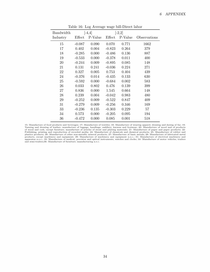
6 APPENDIX
Table 16: Log Average wage bill-Direct labor
Bandwidth [-4,4] [-2,2]Industry Effect P-Value Effect P-Value Observations
15 -0.087 0.090 0.070 0.771 166217 0.402 0.004 -0.823 0.264 37918 -0.285 0.000 -0.486 0.136 88719 -0.533 0.000 -0.378 0.011 40020 -0.244 0.009 -0.895 0.085 14821 0.131 0.241 -0.036 0.224 27122 0.327 0.005 0.753 0.404 43924 -0.376 0.014 -0.435 0.133 63025 -0.592 0.000 -0.684 0.002 58326 0.033 0.802 0.476 0.139 39927 0.836 0.000 1.545 0.664 14828 0.239 0.004 -0.042 0.983 48029 -0.252 0.009 -0.522 0.847 40931 -0.279 0.009 -0.256 0.346 16933 -0.236 0.135 -0.303 0.229 5734 0.573 0.000 -0.205 0.095 19436 -0.472 0.000 0.085 0.001 518
15- Manufacture of food products and beverages; 17- Manufacture of textiles; 18- Manufacture of wearing apparel; dressing and dyeing of fur; 19-Tanning and dressing of leather; manufacture of luggage, handbags, saddlery, harness and footwear; 20- Manufacture of wood and of productsof wood and cork, except furniture; manufacture of articles of straw and plaiting materials; 21- Manufacture of paper and paper products; 22-Publishing, printing and reproduction of recorded media; 24- Manufacture of chemicals and chemical products; 25- Manufacture of rubber andplastics products; 26- Manufacture of other non-metallic mineral products; 27- Manufacture of basic metals; 28- Manufacture of fabricated metalproducts, except machinery and equipment; 29- Manufacture of machinery and equipment n.e.c.; 31- Manufacture of electrical machinery andapparatus n.e.c.; 33- Manufacture of medical, precision and optical instruments, watches and clocks; 34- Manufacture of motor vehicles, trailersand semi-trailers;36- Manufacture of furniture; manufacturing n.e.c.
34

6 APPENDIX
Table 17: Share of exports
Bandwidth [-4,4] [-2,2]Industry Effect P-Value Effect P-Value Observations
15 18.562 0.000 8.700 0.000 166217 29.541 0.000 1.226 0.991 37918 3.974 0.217 -6.990 0.726 88719 -2.308 0.660 -3.937 0.860 40020 0.000 1.000 0.000 1.000 14821 -0.031 0.991 -0.402 1.000 27122 1.101 0.530 -3.089 0.889 43924 -10.436 0.000 -5.966 0.000 63025 -8.066 0.000 -7.297 0.000 58326 1.847 0.009 0.541 0.511 39927 -4.515 0.423 -4.927 0.000 14828 6.032 0.000 -2.537 0.028 48029 8.013 0.001 7.756 0.277 40931 7.635 0.001 1.300 1.000 16933 0.258 0.787 2.061 0.046 5734 0.000 1.000 0.000 1.000 19436 -0.061 0.995 0.852 1.000 518
15- Manufacture of food products and beverages; 17- Manufacture of textiles; 18- Manufacture of wearing apparel; dressing and dyeing of fur; 19-Tanning and dressing of leather; manufacture of luggage, handbags, saddlery, harness and footwear; 20- Manufacture of wood and of productsof wood and cork, except furniture; manufacture of articles of straw and plaiting materials; 21- Manufacture of paper and paper products; 22-Publishing, printing and reproduction of recorded media; 24- Manufacture of chemicals and chemical products; 25- Manufacture of rubber andplastics products; 26- Manufacture of other non-metallic mineral products; 27- Manufacture of basic metals; 28- Manufacture of fabricated metalproducts, except machinery and equipment; 29- Manufacture of machinery and equipment n.e.c.; 31- Manufacture of electrical machinery andapparatus n.e.c.; 33- Manufacture of medical, precision and optical instruments, watches and clocks; 34- Manufacture of motor vehicles, trailersand semi-trailers;36- Manufacture of furniture; manufacturing n.e.c.
35