The effect of head losses evaluation on the analysis …The effect of head losses evaluation on the analysis of pressurized irrigation networks operating on-demand A. Stefopoulou1

Water Utility Journal 3: 3-18, 2012. © 2012 E.W. Publications

The effect of head losses evaluation on the analysis of pressurized irrigation networks operating on-demand

A. Stefopoulou1 and N. Dercas2 Agricultural University of Athens, 75 Iera Odos, 118 55, Athens, Greece, 1 [email protected] 2 [email protected]

Abstract: Collective pressurized irrigation networks operating on-demand are extensively used for the distribution of irrigation water. The importance of the performance analysis of such networks is great both during the networks designing stage and their operational stage. The analysis of such networks is carried out with the use of the Indexed Characteristic Curves for an overview of the network’s performance. The calculation of the head losses is an integral procedure for the performance analysis of such networks. It is widely accepted that the best formula for the calculation of head losses is the Darcy-Weisbach equation with the Colebrook-White formula for the calculation of the friction factor. However, this is not the formula used by the existing software for performance analysis of such networks. In this paper, the effect of various head losses formulas on the Indexed Characteristic Curves is examined. Moreover, due to the fact that the friction factor is not known with certainty in an existing network, a sensitivity analysis was carried out in order to stress the importance of the choice of the value of the roughness parameter. The method is applied in the performance analysis of two Greek collective irrigation networks operating on-demand.

Keywords: collective irrigation networks, performance analysis, friction loss, on-demand networks, sensitivity analysis, indexed characteristic curves

1. INTRODUCTION

Large-scale pressurized irrigation networks operating on-demand have been widely used in the distribution of irrigation water over the last decades. With on-demand systems, the users get greater flexibility allowing the use of more efficient irrigation systems and thus increasing uniformity and irrigation frequency (Rodríguez Díaz et al, 2007; Lamaddalena et al, 2007; Urrestarazu et al, 2009; Carrillo Cobo et al, 2011). The calculation of friction head loss is a central part of both design and analysis of collective irrigation networks. Mathematical modeling is widely used for their performance analysis, where there are generally two approaches: the first one uses the indexed characteristic curves of the network in order to provide analysis at network level, while the second one implements the performance analysis at hydrant level.

The most common software implementing such analysis are ICARE and COPAM. ICARE (CEMAGREF 1983) is a commercial program developed by CEMAGREF in MS-DOS environment. COPAM (Combined Optimization and Performance Analysis Model) is free distributed software, developed by FAO and CHIEAM-Bari Institute in Windows environment (Lamaddalena and Sagardoy 2000). ICARE and COPAM implement both network and hydrant level analysis. For both analyses, computation of the head losses is a vital step. Each of the available analysis software products incorporates a different formula for the calculation of head losses. ICARE uses Calmon and Lechapt formula, and COPAM uses the Darcy equation in combination with Bazin roughness parameter (γ).

In this work, the effect of the formula used for the calculation of head losses on the performance analysis of collective irrigation networks operating on-demand is carried out at network level. It is widely accepted that the best formula for the calculation of the head losses is the Darcy-Weisbach formula with the Colebrook-White formula for the determination of the friction factor. In this paper, we aimed to check how the use of other head losses formulas affects the performance analysis of

4 A. Stefopoulou & N. Dercas

on-demand networks. The comparison between different loss formulas has been extensively addressed in the case of simple pipelines (Allen 1996; Bagarello and Pumo 1992; Hughes and Jeppson 1978; Kamand 1988; Liou 1998; Provenzano et al. 2005); however, such analysis is not adequate in the case of collective irrigation networks operating on-demand. In these networks the user can use his hydrant whenever he wants, depending on the cropping pattern, the meteorological conditions, the farmer’s behavior, etc. Thus the analysis of the operation of such networks is based on a stochastic procedure which determines the pattern of the flows inside the network. Consequently, a large number of flow patterns and demand scenarios should be examined in such networks in order to obtain safe results on the effect of the friction loss formula on the behavior of the network. For the analysis of the networks the Indexed characteristic curves, proposed by Y. Labye (Labye et al. 1975) are usually used and allow us to evaluate their performance. For this reason in this work in order to analyze the effect of friction formulas to network analysis, their impact on the indexed characteristic curves is investigated. Towards this end, two Greek collective irrigation networks are analyzed with various friction loss formulas. In particular, the Darcy –Weisbach equation with the Colebrook – White (DW-CW) and with the Swamee and Jain formulas (DW-SJ) for the calculation of friction factor, the empirical equation of Hazen-Williams (HW), the Darcy equation with Bazin roughness coefficient (DB), the Calmon and Lechapt (CL) formula and the most recent Valiantzas (2008) explicit power formula are compared in terms of network level performance analysis using the Indexed Characteristic Curves. The results given with the examined formulas were compared to the results given with (DW-CW) formula. In this paper, a comparison is carried out between the simulation results given with the various head losses formulas. For the above analysis, the user’s behavior and the irrigation system are known and thus there is no need for field data.

2. METHODS AND MATERIALS

2.1 Performance Analysis of Collective Irrigation Networks Operating On-Demand

The importance of the performance analysis of a collective irrigation network operating on-demand is great both for networks during their designing stage and their operational stage. In the first case, the performance analysis can be implemented in order to avoid over or under dimensioning of the network and to ensure that the designed network will operate successfully for a wide range of discharges in the upstream end of the network. For networks presenting failures during their operation, the performance analysis will define the extent of failure, the particular hydrants that present deficiencies and the magnitude of this deficiency, as well as the saturated pipes.

Generally, the study of a network is accomplished for a given operating point which is defined by the upstream discharge for the peak period (usually the discharge estimated with the Clément’s first formula, QClém) and the optimized piezometric head at the upstream end of the network, Zoptimal. Thus, we do not know how the network will behave for other operational conditions (e.g. other combinations of piezometric head and discharge at the upstream end of the network). In networks operating on-demand, the number and location of open hydrants and consequently the piezometric head and the upstream discharge is not predefined. Thus, the network approach that refers only to a specific operation point (QClém, Zoptimal) presents uncertainties in the case of on-demand collective irrigation networks. By implementing the performance analysis of a pressurized irrigation system that operates on-demand, we aim at investigating how the behavior of the network is affected for various operation conditions (upstream piezometric head Z and upstream discharge Q) and especially for the discharges that appear more frequently.

For the analysis of the collective irrigation networks operating on-demand several models have been developed, which assess their performance at network and at hydrant level. At network level, the analysis is implemented with the indexed characteristic curves (Labye et al. 1975; Bethery et al.

Water Utility Journal 3 (2012) 5

1981; Bethery 1990; CEMAGREF 1983; Lamaddalena and Sagardoy 2000) while at hydrant level several models have been proposed (CEMAGREF 1983; Lamaddalena and Sagardoy 2000; Khadra and Lamaddalena 2010). In contrast to the previous models, other models assume unsteady flow conditions, such as GESTAR (Estrada et al. 2009), FLUCS (Lamaddalena and Perreira 2007) and EPANET (Rossman 2000). Models that implement performance analysis use a random number generator with uniform distribution function for the creation of random configurations with open hydrants.

2.2 Indexed Characteristic Curves (Ci)

In a collective irrigation network operating on-demand each farmer is free to use his hydrant at his own will, leading thus to a large number of possible configurations of open hydrants.

The method of indexed characteristic curves (Ci) offers an overall view of the operation efficiency of a collective irrigation network. The indexes in the characteristic curves represent the percentage of the open hydrants’ configurations that do not present operational failures. The indexed characteristic curves derive from the characteristic curves of the network with the necessary statistical assessment.

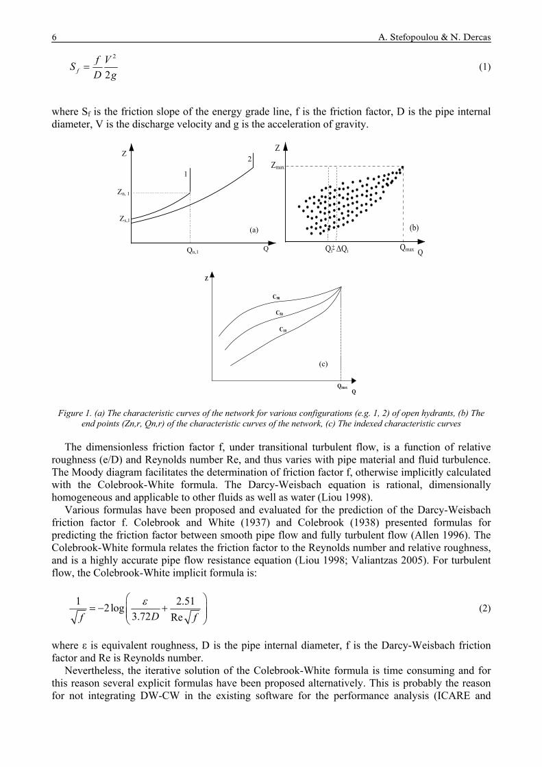
The characteristic curve of a network is strongly dependent on the open hydrants in the network (their number, their nominal discharge, and their location). Let’s assume two characteristic curves (1, 2) of the network corresponding to two configurations of open hydrants (Fig. 1a). The Zs,1 piezometric head at the upstream end of the network is the minimum piezometric head needed in order to start the network deliver water when the configuration (1) of open hydrants occurs in the network. On the other hand, Zn,1 is the piezometric head at the upstream end, needed when all the open hydrants (configuration 1) have their nominal discharge and Qn,1 is the corresponding discharge at the upstream end of the network. The designed curve (1) in Figure 1a is the characteristic curve of the network for the particular combination (1) of open hydrants. Thus, it is obvious that the number of the characteristic curves of a network equals to the number of the combinations of open hydrants. In order to manage the information given by a large number (r) of the characteristic curves of the network, only the pairs (Zn,r, Qn,r), which correspond to the situation when all open hydrants deliver their nominal discharge, will be used for the determination of the Indexed Characteristic Curves (Ci).

The pairs (Zn,r, Qn,r) for all combinations r of open hydrants (Fig.1b) are statistically analyzed and the piezometric heads that allow satisfaction of the 10, 20, ..., 70, 75, 90% of the combinations of open hydrants that require upstream discharge Qi are determined. With this statistical process the indexed characteristic curves are designed (Figure 1c).

For the creation of the indexed characteristic curves, and in order to simulate the random behavior of the farmers, the hydrants in a configuration are opened randomly until the following

equation is fulfilled: irn QQ , , where rnQ , is the total discharge of the simultaneously

operating hydrants in a given configuration r, Qi is the requested simulation discharge at the upstream end of the network and ετ is the value of the accepted tolerance ( = iQ , Fig. 1b).

According to Bethery et al. (1981) the value of the accepted tolerance is equal to the value of the lowest hydrant nominal discharge (Lamaddalena and Sagardoy 2000).

2.3 Friction Loss Formulas

Friction loss evaluation in pipe systems is crucial, not only for the design procedure but also for the network successful operation. In the analysis of collective irrigation networks, the calculation of friction loss is an essential procedure. The Darcy-Weisbach equation is a fundamental equation used for calculating the friction loss:


2

2f

f VS

D g (1)

where Sf is the friction slope of the energy grade line, f is the friction factor, D is the pipe internal diameter, V is the discharge velocity and g is the acceleration of gravity.

Zn, 1

Q

Z

1

2

Qn,1

Zs,1

(a)

Qmax

Zmax

QQi- ΔQi+

Z

(b)

Z

Qmax

C90

C50

C10

Q

(c)

Figure 1. (a) The characteristic curves of the network for various configurations (e.g. 1, 2) of open hydrants, (b) The end points (Zn,r, Qn,r) of the characteristic curves of the network, (c) The indexed characteristic curves

The dimensionless friction factor f, under transitional turbulent flow, is a function of relative roughness (e/D) and Reynolds number Re, and thus varies with pipe material and fluid turbulence. The Moody diagram facilitates the determination of friction factor f, otherwise implicitly calculated with the Colebrook-White formula. The Darcy-Weisbach equation is rational, dimensionally homogeneous and applicable to other fluids as well as water (Liou 1998).

Various formulas have been proposed and evaluated for the prediction of the Darcy-Weisbach friction factor f. Colebrook and White (1937) and Colebrook (1938) presented formulas for predicting the friction factor between smooth pipe flow and fully turbulent flow (Allen 1996). The Colebrook-White formula relates the friction factor to the Reynolds number and relative roughness, and is a highly accurate pipe flow resistance equation (Liou 1998; Valiantzas 2005). For turbulent flow, the Colebrook-White implicit formula is:

1 2.512log

3.72 ReDf f

(2)

where ε is equivalent roughness, D is the pipe internal diameter, f is the Darcy-Weisbach friction factor and Re is Reynolds number.

Nevertheless, the iterative solution of the Colebrook-White formula is time consuming and for this reason several explicit formulas have been proposed alternatively. This is probably the reason for not integrating DW-CW in the existing software for the performance analysis (ICARE and


COPAM). One of the most popular explicit formulas that approximate the Darcy-Weisbach friction factor for turbulent flow was introduced by Swamee and Jain (1976):

2

0.9

5.740.25 log

3.7 Ref

D

(3)

where D is the pipe internal diameter, ε is equivalent roughness and Re is the Reynods number. This explicit formula approximates the implicit Colebrook-White formula within %1 over the

entire range of practical interest: 10-6 < ε/D < 10-2 and 5*103 < Re < 108 (Provenzano et al. 2005). Apart from Swamee and Jain, several explicit formulas have been proposed for the Colebrook-

White formula (Barr 1972; Chen 1985; Churchill 1973; Terzidis 1992). The friction coefficient f, which is explicitly calculated using these formulas, has an accuracy of about 1.5-2.0% (Valiantzas 2008).

Although the Darcy-Weisbach equation provides great accuracy, many engineers use empirical relationships the popularity of which is due to the simple calculation resulting from a single roughness factor for any pipe size or velocity. Furthermore, the use of such power law explicit forms facilitates their integration into numerical models for optimization of pipe networks. Such equation is the Hazen-Williams formula, which is widely used in water delivery systems for closed conduits. In contrast to the Darcy-Weisbach equation, the Hazen-Williams formula is not dimensionally homogeneous and its range of applicability is limited. In SI units the Hazen-Williams formula is:

1.852

4.871f

QS K

D (4)

where Sf is the friction slope of the energy grade line, Q is the volumetric flow rate in m3/s, D is the pipe internal diameter in m, and K is an empirical coefficient, 852.1675.10 HWCK , where CHW is

the friction coefficient for Hazen-Williams. The value of C in Hazen-Williams formula ranges from 80 for extremely rough pipes to approximately 150 for smooth pipes.

Although the Hazen-Williams formula has been successfully used in cases of transitional turbulent flow in smooth pipes, the comparison between DW and HW equations in several papers (Bagarello and Pumo 1992; Hughes and Jeppson 1978; Kamand 1988; Liou 1998; Provenzano et al. 2005) has highlighted the limitations in its application.

Allen (1996) compared the friction estimated with Hazen-Williams and with Moody diagram. According to his results friction factors predicted by Hazen –Williams for C=150 follow the Moody smooth pipe turbulent flow curve closely for 30 000 < Re < 108, and generally underestimate f for Re < 30 000. Moreover, according to his results the Darcy –Weisbach equation is more accurate than the Hazen-Williams for both low velocity and high temperature conditions. Liou (1998) points out that HW equation compared to the DW-CW equation may exceed 40% error if applied outside its applicability range. In particular, the relative error of the HW equation compared to the DW-CW equation is %8 for smooth pipes and increases to 40% for rough pipes. On the other hand, Christensen et al. (2000) state that the HW formula is valid only between smooth and transitional turbulent flow. Allen (1996) states that adjustment of C is necessary with changing pipe velocity and diameter, since it represents a specific relative roughness in the fully turbulent region, and changes with Re and velocity. Valiantzas (2005) demonstrated that there is a strong dependence of C coefficient on pipe diameter and therefore it cannot be considered constant.

Despite the nondimentional homogeneity and the abovementioned limitations, the HW equation remains the most popular pipe flow resistance equation among users.

A more recent formula was proposed by Valiantzas (2008). It is an explicit power law formula that approximates the Darcy-Weisbach combined with the Colebrook-White formula. The


maximum relative error of the proposed formula is about %4 . The proposed formula is extended for all three turbulent regimes and is of the form:

20

5.3

m

f

k QS

D

(5)

where Q, D, and are expressed in SI units.

3.00 012.0 k , ε is the equivalent roughness of the pipe,

1

01133.01

m and

30 100439.0 .

The proposed formula due to its simplicity can be easily adapted in models of hydraulic analysis and optimum design of irrigation networks.

The most common software for the analysis of large scale irrigation networks operating on-demand, namely COPAM and ICARE, incorporate different formulas for the calculation of the friction loss. COPAM software package calculates the friction slope in the pipes using Darcy’s equation (Lamaddalena and Sagardoy 2000):

2 2 50.000857 1 2 0.5fS D Q D (6)

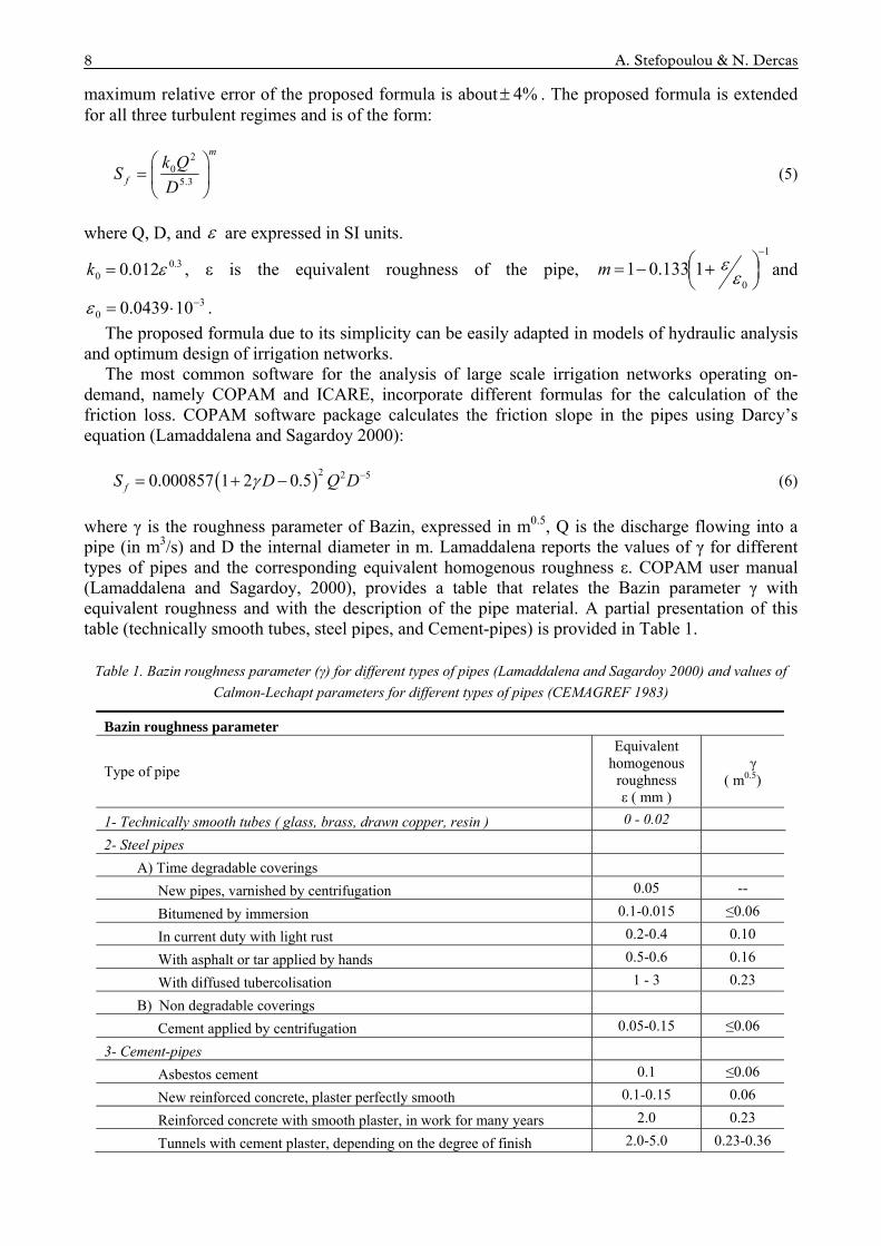
where γ is the roughness parameter of Bazin, expressed in m0.5, Q is the discharge flowing into a pipe (in m3/s) and D the internal diameter in m. Lamaddalena reports the values of γ for different types of pipes and the corresponding equivalent homogenous roughness ε. COPAM user manual (Lamaddalena and Sagardoy, 2000), provides a table that relates the Bazin parameter γ with equivalent roughness and with the description of the pipe material. A partial presentation of this table (technically smooth tubes, steel pipes, and Cement-pipes) is provided in Table 1.

Table 1. Bazin roughness parameter (γ) for different types of pipes (Lamaddalena and Sagardoy 2000) and values of

Calmon-Lechapt parameters for different types of pipes (CEMAGREF 1983)

Bazin roughness parameter

Type of pipe

Equivalent homogenous

roughness ε ( mm )

γ ( m0.5)

1- Technically smooth tubes ( glass, brass, drawn copper, resin ) 0 - 0.02

2- Steel pipes

A) Time degradable coverings

New pipes, varnished by centrifugation 0.05 --

Bitumened by immersion 0.1-0.015 ≤0.06

In current duty with light rust 0.2-0.4 0.10

With asphalt or tar applied by hands 0.5-0.6 0.16

With diffused tubercolisation 1 - 3 0.23

B) Non degradable coverings

Cement applied by centrifugation 0.05-0.15 ≤0.06

3- Cement-pipes

Asbestos cement 0.1 ≤0.06

New reinforced concrete, plaster perfectly smooth 0.1-0.15 0.06

Reinforced concrete with smooth plaster, in work for many years 2.0 0.23

Tunnels with cement plaster, depending on the degree of finish 2.0-5.0 0.23-0.36


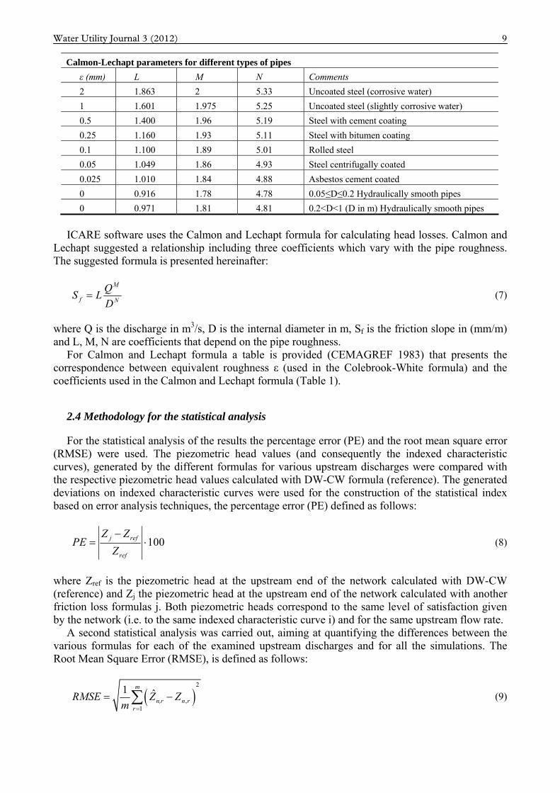
Calmon-Lechapt parameters for different types of pipes

ε (mm) L M N Comments

2 1.863 2 5.33 Uncoated steel (corrosive water)

1 1.601 1.975 5.25 Uncoated steel (slightly corrosive water)

0.5 1.400 1.96 5.19 Steel with cement coating

0.25 1.160 1.93 5.11 Steel with bitumen coating

0.1 1.100 1.89 5.01 Rolled steel

0.05 1.049 1.86 4.93 Steel centrifugally coated

0.025 1.010 1.84 4.88 Asbestos cement coated

0 0.916 1.78 4.78 0.05≤D≤0.2 Hydraulically smooth pipes

0 0.971 1.81 4.81 0.2<D<1 (D in m) Hydraulically smooth pipes

ICARE software uses the Calmon and Lechapt formula for calculating head losses. Calmon and

Lechapt suggested a relationship including three coefficients which vary with the pipe roughness. The suggested formula is presented hereinafter:

M

f N

QS L

D (7)

where Q is the discharge in m3/s, D is the internal diameter in m, Sf is the friction slope in (mm/m) and L, M, N are coefficients that depend on the pipe roughness.

For Calmon and Lechapt formula a table is provided (CEMAGREF 1983) that presents the correspondence between equivalent roughness ε (used in the Colebrook-White formula) and the coefficients used in the Calmon and Lechapt formula (Table 1).

2.4 Methodology for the statistical analysis

For the statistical analysis of the results the percentage error (PE) and the root mean square error (RMSE) were used. The piezometric head values (and consequently the indexed characteristic curves), generated by the different formulas for various upstream discharges were compared with the respective piezometric head values calculated with DW-CW formula (reference). The generated deviations on indexed characteristic curves were used for the construction of the statistical index based on error analysis techniques, the percentage error (PE) defined as follows:

100j ref

ref

Z ZPE

Z

(8)

where Zref is the piezometric head at the upstream end of the network calculated with DW-CW (reference) and Zj the piezometric head at the upstream end of the network calculated with another friction loss formulas j. Both piezometric heads correspond to the same level of satisfaction given by the network (i.e. to the same indexed characteristic curve i) and for the same upstream flow rate.

A second statistical analysis was carried out, aiming at quantifying the differences between the various formulas for each of the examined upstream discharges and for all the simulations. The Root Mean Square Error (RMSE), is defined as follows:

2

,1

1 ˆm

n,r n rr

RMSE Z Zm

(9)


where Zn,r is the piezometric head at the upstream end of the network calculated with the DW-CW

formula in the r simulation and rnZ ,ˆ is the piezometric head at the upstream end of the network in

the same simulation r calculated with the other friction loss formulas, and m is the number of observations which equals to the number of simulations.

2.5 Implemented software

For the implementation of the analysis, a software was created which generates various configurations of open-closed hydrants (using a random number generator and taking into account the probabilities of hydrants utilization) and simulates various flow regimes in the network. Also, it calculates and designs the indexed characteristic curves with the various examined formulas (Stefopoulou and Dercas 2011a; Stefopoulou and Dercas 2011b). The software was implemented with the use of object-oriented programming techniques with Visual Basic.net.

3. APPLICATION

In the present paper the effect of the equation used for the calculation of the friction losses on the performance analysis of collective irrigation networks operating on-demand is examined. As already mentioned, these networks are characterized by high spatial and temporal variability concerning the hydrants’ operation and a probabilistic approach is adopted for the determination of the flow patterns in the network which will be used in the performance analysis. For the analysis the Indexed Characteristic Curves are used. For this reason, two representative Greek collective irrigation networks operating on-demand were used as case studies. The representative pressurized irrigation networks operating on-demand were the Iria network and the Kaluvia-Sochas network. Both networks are located in South Greece.

For Iria network, the piezometric elevation at the upstream end of the network is 46.7m and it serves 318 hydrants with a total irrigated area of 954ha (relatively flat topography, with average altitude 11.5m). The upstream Clément discharge is 411.38L/s and the upstream cumulative discharge is 1908L/s. The total length of pipes is 45179m, while the network is equipped with steel pipes for diameters between 600mm and 800mm, and PVC for diameters equal or less than 500mm.

The piezometric elevation at the upstream end of Kaluvia-Sochas network is 314m and it serves 44 hydrants at 300ha of irrigated area (topography with significant variations in elevations, with average altitude 253.8m). The upstream Clément discharge is 196L/s and the upstream cumulative discharge is 264L/s. The total length of the pipes is 10915m. Steel pipes are used for diameters of 400mm, cement-asbestos pipes for diameters between 300mm and 350mm and PVC pipes for smaller diameters. For both networks the hydrants’ nominal discharge is 6L/s and the required pressure head at hydrant is 20m.

The open hydrant possibility ranges between 0.2 and 0.8. The major crops in Kaluvia-Sochas network are olives and orange trees, while in Iria network are vegetables and citrus.

For these networks, the indexed characteristic curves were calculated with all the examined formulas. The examined equations and formulas for the calculation of the friction losses were the following: Darcy-Weisbach equation with Colebrook-White formula for the calculation of the friction factor (DW-CW), Darcy-Weisbach equation with Swamee and Jain formula (DW-SJ), Hazen-Williams formula (HW), Darcy’s equation with Bazin γ coefficient (DB), Calmon and Lechapt formula (CL) and Valiantzas formula. For the examined networks, the C50 characteristic curves were designed with the abovementioned formulas and were compared afterwards with the indexed characteristic curve C50 designed with the DW-CW formula (reference).

In our study, we examined the networks assuming initially one pipe material (steel and PVC for Iria network and steel, cement asbestos, and PVC for Kaluvia-Sochas network) for all the pipes of the network. Although the assumption of one pipe material for all pipe diameters is not


implemented in practice for economic purposes, it was used in order to present separately the results for each material. Afterwards, the performance of both networks was assessed for the actual distribution of pipe materials inside both networks.

For the DW-CW, DW-SJ, HW and Valiantzas formulas, the coefficients were adopted according to Keller and Bliesner (1990). For Calmon and Lechapt and for the Darcy combined with Bazin parameter, the values for the respective coefficients were taken from the software manuals of ICARE and COPAM that use the abovementioned formulas (CEMAGREF 1983; Lamaddalena and Sagardoy 2000). For PVC we adopted the value used in the example of the COPAM manual (γ=0.06). The values of the various coefficients for the friction loss formulas that were used for each pipe material are presented in Table 2.

Table 2. Parameters adopted for Iria and Kalyvia-Sochas networks

DW-CW and DW-SJ and Valiantzas (2008) (1)

Hazen- Williams (2)

Calmon and Lechapt (3)

Darcy-Bazin roughness parameter γ (4)

PVC ε=0.013 mm C=150 L=0.971 M=1.81 N=4.81

γ=0.06

Steel (old) ε=1.52 mm (*) C=100 L=1.601 M=1.975 N=5.25

γ=0.23

Asbestos-Cement

ε=0.076 mm C=140 L= 1.049 M= 1.86 N=4.93

γ=0.06

(1): According to Keller and Bliesner (1990) (2): According to Keller and Bliesner (1990) (3): According to ICARE software manual (CEMAGREF 1983)

(4): According to COPAM software manual (Lamaddalena and Sagardoy 2000) (*): The value of the roughness parameter proposed by the manufacturers is different from those used in the design.

4. RESULTS AND DISCUSSION

4.1 Performance Analysis Using Indexed Characteristic Curves

In order to assess the performance analysis of the pressurized collective irrigation networks operating on-demand at network level, we implemented 1000 simulations for Iria network and 300 simulations for Kaluvia-Sochas network. The number of the simulations was chosen in order to correspond to the size of the examined network, in particular to the total number of hydrants in the examined network. According to Lamaddalena and Sagardoy (2000), based on the analysis of a large number of irrigation systems, the number of configurations to be tested should be higher than the number of hydrants in the network, unless the number of hydrants is very large (greater than 600 hydrants).

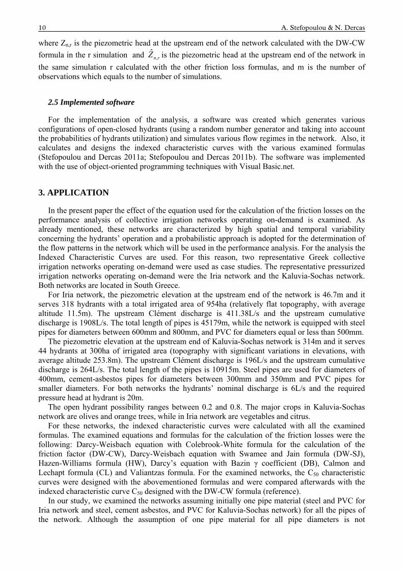
Iria Network: For the statistical analysis of the results at network level, the characteristic curve C50 of the networks was used. Figure 2 presents the indexed characteristic curve C50 for Iria network, when various friction loss formulas are used. All the estimated C50 are compared to the indexed characteristic curve C50 calculated with DW-CW formula. In Fig 2a the network is assumed to be equipped with steel pipes, in Fig 2b the network is assumed to be equipped with PVC pipes, and in Fig 2c the network has the actual pipe materials (steel and PVC) according to the actual situation of the network.

All C50 curves seem to perform well for upstream discharges up to the Clément discharge (QClém=411.38 L/s); however, there are important deviations for greater upstream discharges. The deviations are greater in case the network is equipped with steel pipes. In particular, Darcy with


Bazin roughness parameter seems to overestimate head losses, and the deviation from the DW-CW equation is greater as the examined upstream discharge increases. The Calmon and Lechapt formula underestimates head losses (when steel, PVC pipes are used as well as for the actual situation of the network), especially for discharges near the maximum upstream discharge. The other examined formulas, namely DW-CW, DW-SJ, and Valiantzas (2008) present similar results for all range of upstream discharges. The Hazen-Williams formula underestimates head losses for discharges near the maximum upstream discharge in the case of steel pipes.

Figure 2. C50 characteristic curves for Iria network equipped with (a) Steel pipes, (b) PVC pipes, and (c) Actual situation (Steel and PVC pipes)

The piezometric head values generated by the different formulas for various upstream discharges were compared with the respective piezometric head values calculated with DW-CW formula (reference). The generated deviations were used for the construction of the statistical index based on error analysis techniques and the percentage error (PE) was determined.

The PE of piezometric head was estimated for the values of upstream discharge ranging between 0 and QClém, and for the values of upstream discharge ranging between the QClém and the maximum (cumulative) upstream discharge. For Q<QClem the observed deviations for all formulas and pipe materials were indeed quite low (max PE up to 0.712% for Darcy-Bazin and up to 0.518% for HW).


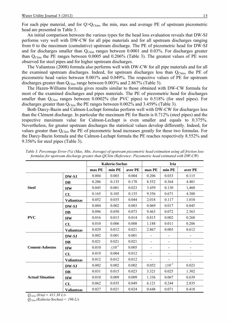
For each pipe material, and for Q>QClem, the min, max and average PE of upstream piezometric head are presented in Table 3.

An initial comparison between the various types for the head loss evaluation reveals that DW-SJ performs very well with DW-CW for all pipe materials and for all upstream discharges ranging from 0 to the maximum (cumulative) upstream discharge. The PE of piezometric head for DW-SJ and for discharges smaller than QClém ranges between 0.0001 and 0.03%. For discharges greater than QClém the PE ranges between 0.0005 and 0.206% (Table 3). The greatest values of PE were observed for steel pipes and for higher upstream discharges.

The Valiantzas (2008) formula also performs well with DW-CW for all pipe materials and for all the examined upstream discharges. Indeed, for upstream discharges less than QClém, the PE of piezometric head varies between 0.001% and 0.049%. The respective values of PE for upstream discharges greater than QClém range between 0.003% and 2.867% (Table 3).

The Hazen-Williams formula gives results similar to those obtained with DW-CW formula for most of the examined discharges and pipes materials. The PE of piezometric head for discharges smaller than QClém ranges between 0.0002% (for PVC pipes) to 0.518% (for steel pipes). For discharges greater than QClém the PE ranges between 0.002% and 3.459% (Table 3).

Both Darcy-Bazin and Calmon-Lechapt formulas perform well with DW-CW for discharges less than the Clément discharge. In particular the maximum PE for Bazin is 0.712% (steel pipes) and the respective maximum value for Calmon-Lechapt is even smaller and equals to 0.375%. Nevertheless, for greater upstream discharges the statistical values develop differently. Indeed, for values greater than QClém the PE of piezometric head increases greatly for these two formulas. For the Darcy-Bazin formula and the Calmon-Lechapt formula the PE reaches respectively 8.552% and 9.356% for steel pipes (Table 3).

Table 3. Percentage Error (%) (Max, Min, Average) of upstream piezometric head estimation using all friction loss

formulas for upstream discharge greater than QClém (Reference: Piezometric head estimated with DW-CW)

Kaluvia-Sochas Iria

max PE min PE aver PE max PE min PE aver PE

DW-SJ 0.004 0.003 0.004 0.206 0.033 0.115

DB 0.206 0.135 0.170 8.552 0.364 4.401

HW 0.045 0.001 0.023 3.459 0.130 1,460

CL 0.165 0.105 0.135 9.356 0.671 4.388

Steel

Valiantzas 0.052 0.035 0.044 2.018 0.117 1.010

DW-SJ 0.004 0.002 0.003 0.069 0.017 0.045

DB 0.096 0.050 0.073 9.463 0.072 2.563

HW 0.016 0.013 0.014 0.815 0.002 0.268

CL 0.010 0.006 0.008 1.188 0.011 0.206

PVC

Valiantzas 0.029 0.012 0.021 2.867 0.003 0.612

DW-SJ 0.002 0.001 0.001 - - -

DB 0.021 0.021 0.021 - - -

HW 0.010 ≤10-3 0.005 - - -

CL 0.019 0.004 0.012 - - -

Cement-Asbestos

Valiantzas 0.012 0.012 0.012 - - -

DW-SJ 0.002 0.002 0.002 0.052 ≤10-3 0.023

DB 0.031 0.015 0.023 3.321 0.025 1.302

HW 0.010 0.009 0.009 1.336 0.067 0.639

CL 0.062 0.035 0.049 6.121 0.244 2.835

Actual Situation

Valiantzas 0.027 0.021 0.024 0.648 0.071 0.418

QClém (Iria) = 411.38 L/s QClém (Kaluvia-Sochas) = 196 L/s


Based on the above results, a second statistical analysis was accomplished, aiming at quantifying the differences between the various formulas for each of the examined upstream discharge. For this reason, the Root Mean Square Error (RMSE) value was calculated, for the piezometric heads at the upstream end of the network generated for each of the examined upstream discharges (50L/s, 100 L/s, 200 L/s,…, 1800 L/s, 1908 L/s) with 1000 simulations.

The RMSE values were estimated for all Zn,r. According to Singh et al. (2004), RMSE values close to zero indicate perfect fit, however, values less than half of the standard deviation (SD) of the observations may be considered low. The estimated values of RMSE for each formula and for each of the examined upstream discharge are compared to the half of the SD of the observations. The results confirm what was observed with the PE. In particular, all examined friction loss formulas perform well with DW-CW for upstream discharges lower than QClém (411.84L/s). DW-SJ and the Valiantzas formula perform well for a range of discharges significantly greater than QClém (up to 1800L/s and 1500L/s) respectively. Darcy-Bazin, HW and CL perform well for a smaller range of upstream discharges (up to 900L/s for DB and HW and 800L/s for CL).

In the case of PVC, Darcy-Bazin, HW and CL perform well for a wider range of upstream discharges (up to 1000L/s, 1600L/s and 1700L/s respectively). DW-SJ performs well for upstream discharges up to 1800L/s (as in the steel pipes) and up to 1400L/s for Valiantzas formula. Finally, for PVC, the worst fit is presented by Darcy-Bazin formula.

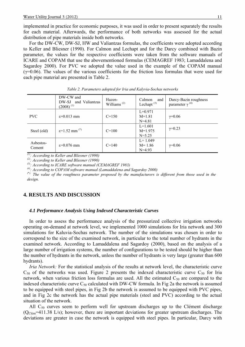
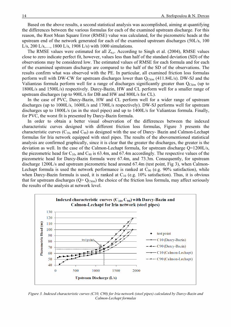
In order to obtain a better visual observation of the differences between the indexed characteristic curves designed with different friction loss formulas, Figure 3 presents the characteristic curves (C10, and C90) as designed with the use of Darcy- Bazin and Calmon-Lechapt formulas for Iria network equipped with steel pipes. The results of the abovementioned statistical analysis are confirmed graphically, since it is clear that the greater the discharges, the greater is the deviation as well. In the case of the Calmon-Lechapt formula, for upstream discharge Q=1200L/s, the piezometric head for C10, and C90 is 63.4m, and 67.4m accordingly. The respective values of the piezometric head for Darcy-Bazin formula were 67.4m, and 73.3m. Consequently, for upstream discharge 1200L/s and upstream piezometric head around 67.4m (test point, Fig 3), when Calmon-Lechapt formula is used the network performance is ranked at C90 (e.g. 90% satisfaction), while when Darcy-Bazin formula is used, it is ranked at C10 (e.g. 10% satisfaction). Thus, it is obvious that for upstream discharges (Q> QClém) the choice of the friction loss formula, may affect seriously the results of the analysis at network level.

Figure 3. Indexed characteristic curves (C10, C90) for Iria network (steel pipes) calculated by Darcy-Bazin and Calmon-Lechapt formulas


Kaluvia-Sochas network: The performance analysis of Kaluvia-Sochas network was also implemented with the various friction loss formulas.

Kaluvia-Sochas network is a small network. The irrigated area is 300ha, while for Iria network the corresponding value was 954ha. As expected, among the results the case of the network equipped with steel pipes presents greater deviations. Once again, there is a differentiation for upstream discharges smaller than QClém (196 L/s) where all friction formulas seem to perform well and for discharges higher than QClém where the deviations from DW-CW are greater. For upstream discharges greater than Clément discharge Darcy-Bazin formula overestimates the friction losses and Calmon-Lechapt formula underestimates the friction losses. All other friction loss formulas, namely DW-SJ, HW, Valiantzas (2008), approximate quite well the curve obtained with DW-CW equation (reference).

The differences observed for steel as well as the differences for the other pipe materials for Q>QClém, are quantified as percentage error (PE) in the Table 3. According to Table 3, for Kaluvia-Sochas network which is a relatively small network, most of the examined friction loss formulas perform well with DW-CW for all combinations of pipe materials and for all upstream discharges (max PE 0.206% for Darcy-Bazin and steel pipes).

4.2 Sensitivity Analysis

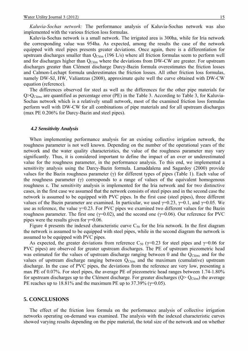
When implementing performance analysis for an existing collective irrigation network, the roughness parameter is not well known. Depending on the number of the operational years of the network and the water quality characteristics, the value of the roughness parameter may vary significantly. Thus, it is considered important to define the impact of an over or underestimated value for the roughness parameter, in the performance analysis. To this end, we implemented a sensitivity analysis using the Darcy-Bazin formula. Lamaddalena and Sagardoy (2000) provide values for the Bazin roughness parameter (γ) for different types of pipes (Table 1). Each value of the roughness parameter (γ) corresponds to a range of values of the equivalent homogenous roughness ε. The sensitivity analysis is implemented for the Iria network and for two distinctive cases, in the first case we assumed that the network consists of steel pipes and in the second case the network is assumed to be equipped with PVC pipes. In the first case (steel pipes), three different values of the Bazin parameter are examined. In particular, we used γ=0.23, γ=0.1, and γ=0.05. We use as reference, the value γ=0.23. For PVC pipes we examined two different values for the Bazin roughness parameter. The first one (γ=0.02), and the second one (γ=0.06). Our reference for PVC pipes were the results given for γ=0.06.

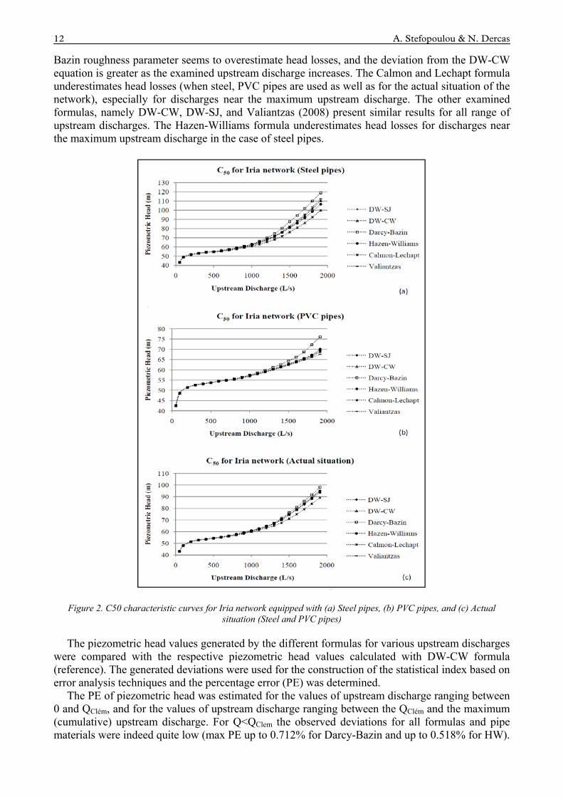
Figure 4 presents the indexed characteristic curve C50 for the Iria network. In the first diagram the network is assumed to be equipped with steel pipes, while in the second diagram the network is assumed to be equipped with PVC pipes.

As expected, the greater deviations from reference C50 (γ=0.23 for steel pipes and γ=0.06 for PVC pipes) are observed for greater upstream discharges. The PE of upstream piezometric head was estimated for the values of upstream discharge ranging between 0 and the QClém, and for the values of upstream discharge ranging between QClém and the maximum (cumulative) upstream discharge. In the case of PVC pipes, the deviations from the reference are very low, presenting a max PE of 0.07%. For steel pipes, the average PE of piezometric head ranges between 1.74-1.80% for upstream discharges up to the Clément discharge. For greater discharges (Q> QClém) the average PE reaches up to 18.81% and the maximum PE up to 37.39% (γ=0.05).

5. CONCLUSIONS

The effect of the friction loss formula on the performance analysis of collective irrigation networks operating on-demand was examined. The analysis with the indexed characteristic curves showed varying results depending on the pipe material, the total size of the network and on whether


the examined upstream discharges were greater than the Clément discharge. The observed deviations when compared to the reference characteristic curve (DW-CW), which is widely accepted as the best formula for calculating friction losses, were greater for higher roughness while they were significantly lower for lower values of the roughness coefficient. For networks which are equipped with various pipe materials (according to the economic optimization) the observed differences in most cases were ranked between the values observed for steel, PVC and Asbestos Cement. Furthermore, the observed deviations relate to the total size of the network; in particular, greater deviations from the reference were observed for larger networks. For discharges lower than QClém, the observed deviations for all pipe materials were low, while the deviations were much greater (up to 9.3%) for steel pipes and greater upstream discharges than the Clément discharge (Q>QClém).

Figure 4. C50 indexed characteristic curves for Iria network calculated by Darcy-Bazin formula and various values for γ roughness parameter. The network is equipped with (a) Steel pipes or (b) PVC pipes.

Based on the above results, for the range 0-QClém all formulas lead to similar indexed characteristic curves. On the contrary, for Q>QClém the adopted friction loss formula affects the accuracy of the analysis. The latter will affect the accuracy of analysis in the case of saturated networks (networks for which the specific continuous discharge or the irrigated area is greater compared to what was foreseen in the initial study of the network) and networks for which the upstream piezometric head will be modified (e.g. reinforcement of pumping station).

The value of the roughness coefficient, in practice, is only known with accuracy for new networks and not for the older ones which are in operation for a long time period. The analysis indicated that the choice of the value for the roughness coefficient contributes significantly to the accuracy of the analysis and to the design of the indexed characteristic curves (for Q>QClém).

Indexed characteristic curves are a valuable tool in view of the performance analysis of pressurized irrigation networks operating on-demand. In this analysis the impact of the choice of friction formula and roughness coefficient on the expected accuracy when designing the indexed


characteristics curves was highlighted. In a nutshell, the aim of the carried out analysis was to reveal the effect of some important issues and parameters that should be taken into account when analyzing the performance of a pressurized collective irrigation network operating on-demand.

REFERENCES

Allen, R.G. (1996). “Relating the Hazen-Williams and Darcy-Weisbach friction loss equations for pressurized irrigation”. Appl. Eng. in Agric, 12(6), 685-693.

Bagarello, V. and Pumo, D. (1992). “Lateral line hydraulics in drip irrigation systems”. Proc., 16th ICID European Regional Conference, Budapest, Hungary.

Barr, D.I.H. (1972). “New forms of equations for the correlation of pipe resistance data”. Proc., Inst. Civ. Eng, 53(20), 383–390. Bethery, J., Meunier, M., and Puech, C. (1981). “Analyse des défaillances et étude du renforcement des réseaux d’irrigation par

aspersion”. Proc. XIe Cong CIID, 36, 297-324. Bethery, J. (1990). “Réseaux collectifs ramifiés sous pression, Calcul et fonctionnement”, Études hydraulique agricole, no 6. Antony,

France. Carrillo Cobo, M.T., Rodríguez-Díaz, J.A., Montesinos, P., López-Luque, R., Camacho-Poyato, E. (2011). “Low energy

consumption seasonal calendar for sectoring operation in pressurized irrigation networks”. Irrig. Science, 29(2), 157-169. CEMAGREF. (1983). “Calcul des réseaux ramifiés sous pression”. No. 506. Antony, France. Chen, J.J.J. (1985). “Systematic explicit solutions of Prandtl and Colebrook-White equations for pipe flow”. Proc. Inst Civ Eng, Part

2, Tech. Note 431, 79, 383–389. Christensen, B.A., Locher, F.A. and Swamee, P.K. (2000). “Discussion of “Limitations and proper use of the Hazen–Williams

equation” by Liou CP”. J. Hydraulic Eng, 126(2), 167–170. Churchill, S.W. (1973). “Empirical expressions for the shear stress in turbulent flow in commercial pipe”. Am. Inst. Chem. Eng. J,

19(2), 375–376. Colebrook, C.F. (1938). “Turbulent flow in pipes, with particular reference to the transition region between the smooth and rough

pipe laws”. J. Inst. Civ. Eng. Lond, 11,133-156. Colebrook, C.F. and White, C.M. (1937). “The reduction of pipe capacity with age”. J. Inst. Civ. Eng. Lond, 10,115-122. Estrada, C., González, C., Aliod, R., and Paño, J. (2009). “Improved Pressurized Pipe Network Hydraulic Solver for Applications in

Irrigation Systems”. J. Irrig. Drain. Eng, 135(4), 421-430. Hughes, T.C. and Jeppson, R.W. (1978). “Hydraulic Friction loss in small diameter plastic pipelines”. Water Resour. Bull,

14(5),1159–1166. Kamand, F.Z. (1988). “Hydraulic friction factors for pipe flow”. J. Irrig. Drain. Eng, 114(2), 311–323. Keller, J. and Bliesner, R.D. (1990). “Sprinkler and trickle irrigation”. Chapman & Hall, New York. Khadra, R. and Lamaddalena, N. (2010). “Development of a Decision Support System for Irrigation Systems Analysis”. Water

Resour. Manag. 24,3279-3297. Labye, Y., Lahaye, J.P., and Meunier, M. (1975). “Utilization des caracteristiques indices”. Proc. Congres de la ICID, Moscou, p30 Lamaddalena, N. and Sagardoy, J.A. (2000). “Performance analysis of on-demand pressurized irrigation Systems”, Irrigation and

Drainage Paper no 59. FAO, Rome. Lamaddalena, N. and Perreira, L.S. (2007). “Pressure-driven modelling for the performance analysis of irrigation systems operating

on demand”. Agric. Water Manag, 90,36-44. Lamaddalena, N., Fratino, U., and Daccache, A. (2007). “On-farm Sprinkler Irrigation Performance as affected by the Distribution

System”. Biosyst Eng, 96 (1), 99–109. Liou, C.P. (1998). “Limitations and proper use of the Hazen-Williams equation”. J. Hydraul Eng, 124(9), 951–954. Provenzano, G., Palau-Salvador, G., and Bralts, V.F. (2005). “Discussion of “Modified Hazen–Williams and Darcy–Weisbach

Equations for Friction and Local Head Losses along Irrigation Laterals” by Valiantzas JD”. J. Irrig. Drain. Eng, 131(4), 342–350. Rodríguez-Díaz, J.A., Camacho Poyato, E., and López Luque, R. (2007). “Model to Forecast Maximum Flows in On-Demand

Irrigation Distribution Networks”. J. Irrig. Drain. Eng, 133(3), 222-231. Rosseman, L.A. (2000). “EPANET User Manual”. US Environmental Protection Agency, Drinking Water Research Division, Risk

Reduction Engineering Laboratory. Cincinnati. Singh, J., Knapp, H.V., and Demissie, M. (2004). “Hydrologic modeling of the Iroquois River watershed using HSPF and SWAT”.

ISWS CR 2004-08. Champaign, Ill: Illinois State Water Survery. Stefopoulou, A., and Dercas, N. (2011a). “Performance Analysis of Large Pressurized Irrigation Networks: Effect of Head Losses

Evaluation”. Proc. VI EWRA Int Symp “Water Engineering and Management in a Changing Environment”, Italy. Stefopoulou, A. and Dercas, N. (2011b). “Investigation of Hydraulic Performance of Irrigation Network Kalyvion-Socha. (Perfecture

of Lakonia, Greece)”. Proc. 7th Greek Conf of the Hellenic Soc. of Agric. Eng., Greece. Swamee, P. and Jain, A. (1976). “Explicit equation for pipe flow problems”. J. Hydraul. Div, 102(5), 657–664. Terzidis, G. (1992). “Discussion of “Simple and accurate friction loss equation for plastic pipe” by von Bernuth RD”. J. Irrig. Drain.

Eng, 118(3), 501–504. Urrestarazu, P., Rodríguez-Díaz, J., Poyato, E., and Luque, R. (2009). “Quality of Service in Irrigation Distribution Networks: Case

of Palos de la Frontera Irrigation District (Spain)”. J. Irrig. Drain. Eng, 135(6), 755–762. Valiantzas, J.D. (2005). “Modified Hazen–Williams and Darcy–Weisbach equations for friction and local head losses along irrigation

laterals”. J. Irrig. Drain. Eng, 131(4), 342–350.


Valiantzas, J.D. (2008). “Explicit Power Formula for the Darcy–Weisbach Pipe Flow Equation: Application in Optimal Pipeline Design”. J. Irrig. Drain. Eng, 134(4), 454-461.

Documents

The effect of head losses evaluation on the analysis …The effect of head losses evaluation on the analysis of pressurized irrigation networks operating on-demand A. Stefopoulou1