Embed Size (px)
Citation preview
The Dirac Equation and the Lorentz Group
Joel G. BroidaUniversity of Colorado, Boulder
Copyright c©2009 by Joel G. Broida. All rights reserved.
February 16, 2009

0

Contents
1 Derivation of the Dirac Equation 1
2 Basic Properties of the Dirac Equation 4
3 Covariance of the Dirac Equation 13
4 Construction of the Matrix S(Λ) 20
5 Easier Approach to the Spinor Solutions 30
6 Energy Projection Operators and Spin Sums 35
7 Trace Theorems 39
8 Decomposing the Lorentz Group 44
9 Angular Momentum in Quantum Mechanics 48
10 Lorentz Invariance and Spin 59
11 The Dirac Equation Again 84
i

ii

The Dirac Equation andThe Lorentz Group
Part I – Classical Approach
1 Derivation of the Dirac Equation
The basic idea is to use the standard quantum mechanical substitutions
p→ −i~∇ and E → i~∂
∂t(1)
to write a wave equation that is first-order in both E and p. This will give us anequation that is both relativistically covariant and conserves a positive definiteprobability density.
We start by assuming that we can factor the relativistic expression E2 =p2 +m2 into the form (we will use units with ~ = c = 1 from now on)
E = α · p + βm (2)
where α and β are to be determined. Note that α and β can not simply benumbers because equation (2) would not even be rotationally invariant. Sincewe must still satisfy E2 = p2 +m2, we have
E2 = (α · p + βm)2 = (αipi + βm)(αjpj + βm)
= αiαjpipj + (αiβ + βαi)pim+ β2m2
=1
2(αiαj + αjαi)pipj + (αiβ + βαi)pim+ β2m2
where we used the fact that pipj = pjpi. This requires that
1
2(αiαj + αjαi) = δij (3a)
αiβ + βαi = 0 (3b)
β2 = I (3c)
Since pure numbers commute, let us assume that the αi and β are matrices.Using equations (3), we define the matrices
γi := βαi and γ0 := β.
Then
2δij = αiαj + αjαi = β2αiαj + β2αjαi = −βαiβαj − βαjβαi
= −(γiγj + γjγi)
1

and0 = αiβ + βαi =⇒ 0 = βαiβ + β2αi = γiγ0 + γ0γi
and hence we haveγµγν + γνγµ = {γµ, γν} = 2gµν (4)
where we are using the metric g = diag(1,−1,−1,−1), i.e.,
(gµν) =
1−1
−1−1
= (gµν).
Matrices satisfying equation (4) are said to form a Clifford algebra. Note inparticular that we also have
(αi)2 = I.
From equation (3b) we see that βαiβ = −αi and αiβαi = −β. Usingthe cyclic property of the trace along with β2 = (αi)2 = I, these imply thattrβ = trαi = 0. Now let λ be an eigenvalue of β. Then βv = λv impliesv = β2v = λβv = λ2v and therefore λ = ±1. But the trace of a matrixis the sum of its eigenvalues (i.e., if P−1AP = D = diag(λ1, . . . , λn), thentrA = trP−1AP = trD), and hence it follows that β must be even-dimensional,with an exactly analogous result for αi.
Now, the energy operator E must have real eigenvalues and hence must beHermitian. Since p is already Hermitian, it follows from equation (2) that αand β must be Hermitan matrices. The most general 2× 2 Hermitian matrix isof the form
[z x− iy
x+ iy t
]= xσ1 + yσ2 +
z
2(σ3 + I)− t
2(σ3 − I)
where
σ1 =
[1
1
]σ2 =
[−i
i
]σ3 =
[1−1
]I =
[1
1
].
Hence the most general 2 × 2 Hermitian matrix is a linear combination of thethree (Hermitan) Pauli matrices and the identity matrix. (It is easy to see thatif we write σ0 := I, then
0 =
3∑
i=0
ciσi =
[c0 + c3 c1 − ic2c1 + ic2 c0 − c3
]
implies that all of the ci must equal zero, and hence the four matrices σ0, . . . , σ3
are linearly independent and form a basis for the space M2(C).) If we take theα’s to be linear combinations of the σ’s, then this leaves β = I. But I commuteswith everything, so it certainly can’t anticommute with the α’s. Thus we assumethat the γ’s are in fact 4× 4 matrices.
2
In block matrix form, we define the standard representation to be
β =
[1−1
]. (5a)
Since the α’s are Hermitan, we have
0 = αiβ + βαi =
[A BB† C
] [1−1
]+
[1−1
] [A BB† C
]
=
[2A
−2C
]
so that A = C = 0 and we can choose
α =
[0 σ
σ 0
]. (5b)
In other words, we take the standard representation of the gamma matrices tobe (in block matrix form)
γ0 =
[1 00 −1
]γ =
[0 σ
−σ 0
]. (6)
I leave it as an exercise to show directly that if {γµ} is a set of matricessatisfying {γµ, γν} = 2gµν , then γµ 6= γν for µ 6= ν and the γ’s are linearlyindependent.
Next, recall that the gradient is defined by ∇ = ∂/∂x so ∇i = ∂/∂xi = ∂i
and we write∂µ = (∂0, ∂i) = (∂0,−∂i) = (∂0,−∇)
along with ∂µ = (∂0,+∇). The quantum mechanical operators are E = i∂0 andpi = −i∂i or p = −i∇, and hence we can write
pµ = +i∂µ. (7)
Then the operators in the Dirac equation become i∂0 = −iαi∂i + βm so thatmultiplying through by γ0 this is iγ0∂0 = −γi∂i +m (the I multiplying the m isunderstood) or simply iγµ∂µ −m = 0. As a very convenient notational device,we introduce the “Feynman slash” notation for the contraction of any 4-vectoraµ with the gamma matrices γµ in which we write
/a := γµaµ.
Using this notation, the Dirac equation is then written as(iγµ ∂
∂xµ−m
)ψ(x) = 0
or simply(i/∂ −m)ψ(x) = 0. (8)
3

Equivalently, we can write this in the form
(/p−m)ψ(x) = 0. (9)
It is extremely important to realize that now the wavefunction ψ is a 4-component column vector, generally referred to as a Dirac spinor. We willsee that these four degrees of freedom allow us to describe both positive andnegative energy solutions, each with spin 1/2 either up or down. The negativeenergy solutions are interpreted as describing positive energy antiparticles. Inother words, the Dirac equation describes spin 1/2 electrons and positrons (aswell as the other leptons and quarks).
Note that γ0† = γ0 and γi† = (βαi)† = αi†β† = αiβ = β2αiβ = βγiβ =γ0γiγ0 and hence in general we have the very useful result
㵆 = γ0γµγ0 (10)
which is independent of the representation of the gamma matrices. We will seethat rather than ψ†, it turns out that the useful quantity will be
ψ := ψ†γ0.
Taking the adjoint of (8) yields
0 = ψ†(−i㵆←−∂µ −m) = ψ†(−iγ0γµγ0←−∂µ − γ0γ0m)
where the symbol←−∂µ means that the derivative acts to the left. Multiplying
this from the right by γ0 we have ψ†γ0(−iγµ←−∂µ −m) = 0 and hence ψ satisfiesthe equation
ψ(x)(i←−/∂ +m) = 0. (11)
To get a probability current, we multiply (8) from the left by ψ and (11)from the right by ψ and add to obtain
i(ψγµ∂µψ + ∂µψγµψ) = 0
or simply∂µ(ψγµψ) = 0. (12)
Hence the probability current is given by
jµ = ψγµψ
and it satisfies the continuity equation ∂µjµ = 0.
2 Basic Properties of the Dirac Equation
Before we turn to the issue of covariance under Lorentz transformations, let ustake a look at some of the basic properties of the Dirac equation.
4

To begin with, note that equation (8) has solutions of the form
ψ(x, t) = u(p)e−ipµxµ
where u(p) is a 4-component spinor that must satisfy
(/p−m)u(p) = 0.
This is a set of four homogeneous linear equations, and it will have a nontrivialsolution if and only if the matrix (/p − m) does not have an inverse. Fromequation (4) we see that in general for any 4-vectors aµ, bµ we have
/a/b + /b/a = (γµγν + γνγµ)aµbν = 2a · b
so that /p/p = p2. It is then easy to see
(/p+m)(/p−m) = p2 −m2
so that a formal inverse to (/p−m) is (p2 −m2)−1(/p+m). But if this inverse isnot to exist, we must have p2 −m2 = 0 so that (p0)2 − p2 = m2 or
E = ±√
p2 +m2.
In other words, the Dirac equation allows solutions with negative energy, andfree particles have an energy E with |E| ≥ m.
Since negative energy states have never been observed, we have to somehowexplain their absence. (Such states would have an acceleration in a directionopposite to the applied force. If a particle is accelerated from rest to an energyE =
∫F · dr = ±m
∫a · v dt = ±m
∫(dv/dt) · v dt = ±(m/2)
∫(dv2/dt) dt < 0,
then we must have F = −ma.) While the completely correct answer lies inthe formalism of relativistic quantum field theory, at the time Dirac postulatedthat all negative energy states were already filled by an infinite sea of negativeenergy electrons, and the Pauli principle prevented any positive energy electronfrom falling down into the negative sea. If such a negative energy electron werehit by a sufficiently energetic photon, it could make the transition to a positiveenergy state, leaving behind a “hole” that we would perceive as a positive energypositively charged electron, a “positron.”
In any case, what can we say about the constants of the motion? Definingthe Dirac Hamiltonian
HD = α · p + βm
we can write the Dirac equation as
HDψ = i∂ψ
∂t
which is of the same form as the Schrodinger equation. Then this has a formalsolution with time dependence that goes as e−iHDt, and we can define operators
5

O in the Heisenberg picture with the usual equation of motion that allows usto look for conserved quantities:
dOdt
= −i[O, HD].
Let us first look at the orbital angular momentum L = r × p. Using thecommutator identity
[ab, c] = a[b, c] + [a, c]b
along with the fundamental commutation relations [pi, pj ] = 0 and [xi, pj ] =iδij , we compute (using a sloppy summation convention)
[Li, HD] = εijk[xjpk, HD] = εijk(xj [pk, HD] + [xj , HD]pk).
But[pk, HD] = [pk, αlpl + βm] = 0
while
εijk[xj , HD]pk = εijk[xj , αlpl + βm]pk = iεijkδjl α
lpk = i(α× p)i
so that[L, HD] = i(α× p).
This shows that the orbital angular momentum is not a constant of the motion.Now consider the matrix operator
σ′ =
[σ 00 σ
]
where the Pauli matrices obey the relations
[σi, σj ] = 2iεijkσk (13a)
σiσj = δij + iεijkσk (13b)
and therefore also (σi)2 = 1. These show that the operator S defined by S =
σ′/2 satisfies[Si, Sj ] = iεijkSk
and hence is an angular momentum operator. Since σ2 = σ ·σ = 3, we see that
S2 =3
4
[1 00 1
]
so that s(s + 1) = 3/4 implies that s = 1/2. Thus S is the spin operator fora particle of spin 1/2. However, we still haven’t connected this to the Diracequation.
Recall that the standard representation for α and β is
α =
[0 σ
σ 0
]and β =
[1 00 −1
]
6
so it it easy to see that
[σ′i, αj ] = 2iεijkαk and [σ′
i, β] = 0.
Hence we find that
[σ′i, HD] = [σ′
i, αjpj + βm] = 2iεijkαkp
j = 2i(p×α)i
or, alternatively,[S, HD] = −i(α× p).
Combining this with our previous result for L we see that the operator
J := L + S
is conserved because [J, HD] = 0, and furthermore it is an angular momentumoperator because
[Ji, Jj ] = iεijkJk.
I leave it as an exercise to show that [J2, HD] = [S2, HD] = 0, and hence theoperatorsHD,J,J
2 and S2 are a mutually commuting set. This then shows thatthe Dirac equation represents a particle with conserved total angular momentumJ = L + S and with spin equal to 1/2.
Now let’s take a look at the interaction of a Dirac particle with the electro-magnetic field. Since quantum mechanics is formulated using the Hamiltonian,we need to know what the canonical momentum is for a particle of charge e in anelectromagnetic field. By definition, this is p = ∂L/∂q where L = L(q, q, t) is theLagrangian of the system. In this case, the answer is we make the replacements
p→ p− eA and E → E − eφ (14)
where A is the magnetic vector potential and φ is the electric potential. Forthose who are interested, let me somewhat briefly go through the derivation ofthis result.
In a proper derivation of the Lagrange equations of motion, one starts fromd’Alembert’s principle and derives Lagrange’s equation
d
dt
∂T
∂qi− ∂T
∂qi= Qi (15)
where T = T (qi, qi) is the kinetic energy and Qi is a generalized force. In theparticular case that Qi is derivable from a conservative force, then we haveQi = −∂V/∂qi. Since the potential energy V is assumed to be independent ofqi, we can replace ∂T/∂qi by ∂(T −V )/∂qi and we arrive at the usual Lagrangeequation
d
dt
∂L
∂qi− ∂L
∂qi= 0 (16)
7
where L = T − V . However, even if there is no potential function V , we canstill arrive at this result if there exists a function U = U(qi, qi) such that thegeneralized forces may be written as
Qi = −∂U∂qi
+d
dt
∂U
∂qi
because defining L = T − U we again arrive at equation (16). The functionU is called a generalized potential or a velocity dependent potential.We now seek such a function to describe the force on a charged particle in anelectromagnetic field.
Recall from electromagnetism that the Lorentz force law is given by
F = e(E + v ×B)
or
F = e(−∇φ− ∂A
∂t+ v × (∇ ×A)
)
where E = −∇φ − ∂A/∂t and B = ∇ ×A. Our goal is to write this in theform
Fi = − ∂U∂xi
+d
dt
∂U
∂xi
for a suitable U . All it takes is some vector algebra. We have
[v × (∇ ×A)]i = εijkεklmvj∂lAm = (δl
iδmj − δm
i δlj)v
j∂lAm
= vj∂iAj − vj∂jAi = vj∂iAj − (v ·∇)Ai.
But xi and xj are independent variables (in other words, xj has no explicitdependence on xi) so that
vj∂iAj = xj ∂Aj
∂xi=
∂
∂xi(xjAj) =
∂
∂xi(v ·A)
and we have
[v × (∇ ×A)]i =∂
∂xi(v ·A)− (v ·∇)Ai.
But we also have
dAi
dt=∂Ai
∂xj
dxj
dt+∂Ai
∂t= vj ∂Ai
∂xj+∂Ai
∂t= (v ·∇)Ai +
∂Ai
∂t
so that
(v ·∇)Ai =dAi
dt− ∂Ai
∂t
and therefore
[v × (∇×A)]i =∂
∂xi(v ·A)− dAi
dt+∂Ai
∂t.
8
But we can write Ai = ∂(vjAj)/∂vi = ∂(v ·A)/∂vi which gives us
[v × (∇×A)]i =∂
∂xi(v ·A)− d
dt
∂
∂vi(v ·A) +
∂Ai
∂t.
The Lorentz force law can now be written in the form
Fi = e
(− ∂φ∂xi− ∂Ai
∂t+ [v × (∇×A)]i
)
= e
(− ∂φ∂xi− ∂Ai
∂t+
∂
∂xi(v ·A)− d
dt
∂
∂vi(v ·A) +
∂Ai
∂t
)
= e
[− ∂
∂xi(φ− v ·A)− d
dt
∂
∂vi(v ·A)
].
Since φ is independent of v we can write
− d
dt
∂
∂vi(v ·A) =
d
dt
∂
∂vi(φ− v ·A)
so that
Fi = e
[− ∂
∂xi(φ− v ·A) +
d
dt
∂
∂vi(φ− v ·A)
]
or
Fi = − ∂U∂xi
+d
dt
∂U
∂xi
where U = e(φ− v ·A). This shows that U is a generalized potential and thatthe Lagrangian for a particle of charge e in an electromagnetic field is
L = T − eφ+ ev ·A (17a)
or
L =1
2mv2 − eφ+ ev ·A. (17b)
Since the canonical momentum is defined as pi = ∂L/∂qi = ∂L/∂vi we nowsee that
pi = mvi + eAi
orp = mv + eA.
Therefore, in the absence of the electromagnetic field the Hamiltonian is H =p2/2m where p = mv, so if the field is present we must now write
H =(p− eA)2
2m. (18)
(You can also think of this as writing v = (p − eA)/m and now making thissubstitution in the definition H = piqi −L so that H = H(q, p).) Furthermore,the energy of the particle now has an additional term −eφ due to the work in
9

moving against the E field, so the energy operator must be E−eφ (the magneticfield B does no work since the force is perpendicular to the velocity).
We can combine these results into a single relativistic 4-momentum by mak-ing the replacement
pµ → pµ − eAµ (19)
where the 4-potential is given by Aµ = (φ,A). The Dirac Hamiltonian nowbecomes
HD = α · p− eα ·A + βm+ eφ+ V (20)
where V is any additional potential that may be acting on the particle. Makingthe replacement (19) in the case where V = 0, the Dirac equation becomes
(/p− e /A−m)ψ = 0. (21)
One of the great triumphs of the Dirac equation is that it gives us the correctgyromagnetic ratio with g = 2 for the electron, and the correct form of the spin-orbit coupling including the Thomas factor of 1/2. We are now in the positionto prove these results.
To see all of this, first write the Dirac equation as two coupled spinor equa-tions, and then take the non-relativistic limit. Using the Hamiltonian (20) andthe standard representation for the Dirac matrices, the Dirac equation can bewritten in the form
i∂t
[ϕχ
]= α · (p− eA)
[ϕχ
]+ βm
[ϕχ
]+ eφ
[ϕχ
]
where p = −i∇ and α and β are given by equations (5). This is equivalent tothe coupled equations
i∂tϕ = σ · (p− eA)χ+ (eφ+m)ϕ (22a)
i∂tχ = σ · (p− eA)ϕ+ (eφ−m)χ (22b)
In the non-relativistic limit, m is the largest energy term in this equation, sowe write [
ϕχ
]= e−imt
[ϕχ
]
where the 2-component spinors ϕ and χ are relatively slowly varying functionsof time.
Using (22b) we have
i∂tχ = σ · (p− eA)ϕ+ (eϕ− 2m)χ ≈ 0.
Since eϕ≪ 2m this becomes
χ =1
2mσ · (p− eA)ϕ
10
and since p ≈ mv, we see that χ ∼ O(v/c)× ϕ. (Remember we are using unitswhere c = 1.) Because of this, we refer to χ as the “small component” and ϕas the “large component” of ψ.
Substituting the above expression for χ into (22a) we obtain
i∂tϕ =1
2m[σ · (p− eA)]2ϕ+ eφϕ.
From equation (13b) we have the very useful result
(σ · a)(σ · b) = a · b + iσ · (a× b). (23)
Writing π := p− eA and using (23) we have
(σ · π)2 = π · π + iσ · (π × π).
Note that π is a differential operator so that π ×π 6= 0. In particular, we have
π × π = (p− eA)× (p− eA) = −e(A× p + p×A)
= ie(A×∇ + ∇×A)
so that
(π × π)ϕ = ie[A×∇ϕ+ ∇× (Aϕ)] = ie(∇×A)ϕ = ieBϕ.
Therefore we have
i∂ϕ
∂t=
(p− eA)2
2mϕ− e
2m(σ ·B)ϕ+ eφ ϕ. (24)
This is the non-relativistic Pauli equation for a particle of spin 1/2 in an elec-tromagnetic field. Note that the magnetic moment is predicted to be e/2m (inother units, this is e~/2mc), and thus we automatically have g = 2 exactly.(There are higher order corrections to this that follow from the formalism ofQED.)
(A sketch of the classical theory is as follows: The orbital magnetic momentof a current loop is
µl =I
c× area
where
I =charge
time=
charge
dist/vel=
e
2πr/v=
ev
2πr
so that
µl =ev
2πrcπr2 =
evr
2c=
eL
2mc.
As vectors, this is
µl =e
2mcL
where the ratio of µ to L is called the gyromagnetic ratio γ.
11

Generalizing this, we make the definition
µ = ge
2mcJ
where g is a constant. For an electron we have J = S = (~/2)σ and, fromexperiment, g is very close to 2 so that
µs =e~
2mcσ
with an energy −µs ·B = −(e~/2mc)(σ ·B).)Now for the spin-orbit coupling in a hydrogen atom (with a nucleus of essen-
tially infinite mass). To describe this, we first rewrite equations (22) by lookingfor energy eigenstates ψ(x, t) = e−iEtψ(x). Then we can write equations (22)as
Eϕ = σ · (p− eA)χ+ (eφ+m)ϕ (25a)
Eχ = σ · (p− eA)ϕ+ (eφ−m)χ (25b)
where now ϕ and χ are independent of time. With A = 0 (there is no externalfield) and letting eφ = V , the second of these may be written as
χ = (E − V +m)−1(σ · p)ϕ.
(Be sure to remember that p = −i∇ so the order of factors is important becauseV is not a constant.) Let E = E′ +m so that
χ = (E′ − V + 2m)−1(σ · p)ϕ.
Putting this into (25a) we can write
E′ϕ =(σ · p)
2m
(1 +
E′ − V2m
)−1
(σ · p)ϕ+ V ϕ
and to first order this is
E′ϕ =(σ · p)
2m
(1− E′ − V
2m
)(σ · p)ϕ+ V ϕ.
From [p, V ] = −i∇V we have pV = V p− i∇V so our equation becomes
E′ϕ =
[1
2m
(1− E′ − V
2m
)(σ · p)2 − i
4m2(σ ·∇V )(σ · p)
]ϕ+ V ϕ.
Using (23) we have (σ · p)2 = p2 and
(σ ·∇V )(σ · p) = ∇V · p− iσ · (∇V × p)
so that
E′ϕ =
[(1− E′ − V
2m
)p2
2m− i
4m2∇V · p− 1
4m2σ · (∇V × p)
]ϕ+ V ϕ.
12

We assume spherical symmetry for V (for the hydrogen atom V = −e2/r) sothat
∇V =dV
drr =⇒ ∇V · p = −idV
dr
∂
∂r
and
∇V × p =dV
drr× p =
1
r
dV
drr× p =
1
r
dV
drL.
Therefore, since S = σ/2 we have
E′ϕ =
[(1− E′ − V
2m
)p2
2m+ V
]ϕ− 1
4m2
dV
dr
∂ϕ
∂r− 1
2m2
1
r
dV
dr(S · L)ϕ.
Finally, since E is the total energy, we can write E′ − V ≈ p2/2m to arrive atthe Schrodinger-like (two-component) equation
[p2
2m− p4
8m3+ V − 1
4m2
dV
dr
∂
∂r− 1
2m2
1
r
dV
dr(S · L)
]ϕ = E′ϕ. (26)
The second term is a relativistic correction to the kinetic energy, and thefourth term is called the “Darwin term.” It is essentially due to the fact that arelativistic particle can’t be localized to within better than its Compton wave-length ~/mc, and as a result the effective potential is really smeared out. Andlastly, the final term is the spin-orbit coupling including the factor of 1/2 fromThomas precession. (Very roughly, here is the non-relativistic approach: Theelectron sees a current due to the relative motion of the nucleus, and this is thesource of a magnetic field
B = (−e/c)v× r/r3 = (e/mc)p× r/r3 = (−e/mcr3)L.
Then there will be an interaction energy term in the Hamiltonian that is
−µ ·B = −(e/mc)(−e/mcr3)S · L = (e2/m2c2r3)S · L.
With c = 1 and V = −e2/r, this is the same as (1/m2r)(dV/dr)(S·L). However,this answer is off by a factor of 1/2 due to Thomas precession, and this isautomatically taken into account in equation (26).)
3 Covariance of the Dirac Equation
We now turn our attention to the covariance of the Dirac equation under aLorentz transformation
xµ → x′µ = Λµνx
ν . (27)
Note that x′µx′µ = ΛµνΛµ
αxνxα := xνxν which implies
ΛµνΛµ
α = ΛT αµΛµ
ν = δαν = gα
ν . (28)
13

This shows that ΛT αµ = Λ−1α
µ so that Λ is an orthogonal transformation, i.e.,
(Λ−1)αµ = (ΛT )αµ = Λµα.
Equation (28) can also be written as (ΛT )αµΛµν = (ΛT )αµ g
µβΛβν = gαν ormost simply as
ΛT gΛ = g (29)
which is frequently taken as the definition of a Lorentz transformation Λ. Notein particular that since ΛT = Λ−1 we also have ΛgΛT = g and therefore
gαβ = gµνΛµαΛν
β = ΛναΛνβ = Λα
νΛβν. (30)
Since ∂µ is a 4-vector we have ∂′µ = Λµν∂ν , and inverting this yields ∂α =
(Λ−1)αµ∂′µ = Λµ
α∂′µ. (That ∂µ is a true 4-vector follows from equation (27).
We first have xα = (Λ−1)αµx
′µ so that ∂xα/∂x′µ = (Λ−1)αµ = Λµ
α. Therefore
∂′µ =∂
∂x′µ=∂xα
∂x′µ∂
∂xα= Λµ
α ∂
∂xα= Λµ
α∂α
which shows that ∂µ indeed has the correct transformation properties.) Apply-ing this to the Dirac equation we have
0 = (iγµ∂µ −m)ψ(x) = (iγµΛαµ∂
′α −m)ψ(Λ−1x′)
Let us define γ′α = Λαµγ
µ and observe that (using equation (30))
{γ′α, γ′β} = ΛαµΛβ
ν{γµ, γν} = 2ΛαµΛβ
νgµν = 2Λα
µΛβµ = 2gαβ
so the γ′µ also obey equation (4). As we will prove below, Pauli’s Funda-
mental Theorem shows that given any two sets of matrices {γµ} and {γ′µ}satisfying the Clifford algebra (4), there exists a nonsingular matrix S such that
γ′α = Λαµγ
µ = S−1γαS. (31)
(That γ′α = Λαµγ
µ is simply our definition of γ′α — it has nothing to do withthe general conclusion of Pauli’s theorem.)
We now use this result to write
0 = (iγµΛαµ∂
′α −m)ψ(Λ−1x′) = (iS−1γαS∂′α −m)ψ(Λ−1x′)
= (iS−1γαS∂′α − S−1Sm)ψ(Λ−1x′)
= S−1(iγα∂′α −m)Sψ(Λ−1x′)
which then implies0 = (i/∂
′ −m)ψ′(x′)
where we have defined the transformed wave function
ψ′(x′) := S(Λ)ψ(Λ−1x′) = S(Λ)ψ(x). (32)
14
It is important to realize that the gamma matrices themselves do not changeunder a Lorentz transformation. Everything will be fine if we can show that thetransformed wave function ψ′(x′) has the correct physical interpretation in theprimed frame, i.e., we want to show that jµ → j′µ = Λµ
νjν . Before doing this
however, we first go back and prove Pauli’s fundamental theorem because wewill need some of the results that we prove along the way.
First of all, we want 16 linearly independent 4×4 matrices. Since {γµ, γν} =2gµν , it follows that (γµ)2 = ±1, and hence we need only consider products ofdistinct gamma matrices. Note that from the binomial theorem, the number ofcombinations of n objects taken one at a time, two at a time, . . . , n at a time is
(n
1
)+
(n
2
)+ · · ·+
(n
n
)=
n∑
k=1
(n
k
)=
n∑
k=0
(n
k
)1k1n−k − 1
= (1 + 1)n − 1 = 2n − 1.
In our case we have n = 4, so there are 15 possible distinct combinations of thegamma matrices taken one, two, three and four at a time. Together with theidentity matrix, this gives us the 16 matrices Γi defined by
I Γ1
γ0 iγ1 iγ2 iγ3 Γ2 − Γ5
γ0γ1 γ0γ2 γ0γ3 γ1γ2 γ1γ3 γ2γ3 Γ6 − Γ11
iγ0γ1γ2 iγ0γ1γ3 iγ0γ2γ3 iγ1γ2γ3 Γ12 − Γ15
iγ0γ1γ2γ3 Γ16
The factors of i are included so that
(Γi)2 = +1. (33)
Using the fact that the gamma matrices anticommute, it is easy to see thatΓiΓj = ±ΓjΓi, and in fact
ΓiΓj = aijΓk where aij = ±1,±i. (34)
If Γj 6= Γ1, there exists at least one Γi such that
ΓiΓjΓi = −Γj. (35)
In particular, we have
Γj , 2 ≤ j ≤ 5 =⇒ Γi = Γ16
Γj , 6 ≤ j ≤ 11 =⇒ Γi = whichever of the Γ2,Γ3,Γ4 or Γ5 thatcontains one of the same γµ’s that is in Γj
Γj , 12 ≤ j ≤ 15 =⇒ Γi = Γ16
Γj = Γ16 =⇒ Γi = Γ2,Γ3,Γ4 or Γ5 all work
(36)
15

Note that equations (33) and (35) together imply
tr Γj = 0 for j 6= 1. (37)
We still have to show that the Γi’s are linearly independent. There are (atleast) two ways to show this. First, suppose that x1Γ1+· · ·+x16Γ16 = 0. Takingthe trace shows that x1 = 0 since tr Γ1 = 4 6= 0 and tr Γj = 0 for j 6= 1. From(35) we have ΓiΓj = −ΓjΓi (for j 6= 1), so it follows that tr ΓiΓj = 0 as longas i 6= j. Therefore, multiplying x2Γ2 + · · ·+ x16Γ16 = 0 by Γi and taking thetrace implies that xi = 0 for each i = 2, . . . , 16. Therefore the Γ’s are linearlyindependent and form a basis for the space of 4× 4 complex matrices.
The second way to see this is to also start from∑16
k=1 xkΓk = 0. Multiplyingby Γm we obtain
0 = xmI +∑
k 6=m
xkΓkΓm = xmI +∑
k 6=m
xkakmΓn
where Γn 6= I since k 6= m. (If k 6= m and ΓkΓm = akmI, then Γk = akmΓm
which is impossible.) Taking the trace now shows that xm = 0.In either case, we see that any 4×4 complex matrixX has a unique expansion
X =∑xiΓi, since if we also have X =
∑yiΓi, then
∑(xi − yi)Γi = 0 which
implies that xi = yi since the Γ’s are linearly independent. Note also that theexpansion coefficients xi are determined by
tr(XΓj) = xj tr I = 4xj
or
xi =1
4tr(XΓi). (38)
It is also true that ΓiΓj = aijΓk where Γk is different for each j (and fixed i).To see this, suppose ΓiΓj = aijΓk and ΓiΓj′ = aij′Γk. Multiplying from the leftby Γi shows that Γj = aijΓiΓk and Γj′ = aij′ΓiΓk which implies (1/aij)Γj =(1/aij′)Γj′ or Γj = (aij/aij′)Γj′ which contradicts the linear independence ofthe Γ’s if j 6= j′.
The following theorem is sometimes called Schur’s lemma, but technicallythat designation refers to irreducible group representations. In this case, thesixteen matrices Γi form a basis for what is called the Dirac algebra, whichis a particular type of non-commutative ring. It can be shown that the onlyirreducible representation of the Dirac algebra is four-dimensional, but to do sowould lead us too far astray from our present purposes.
Theorem 1. If X ∈ M4(C) and [X, γµ] = 0 for all µ, then X = cI for somescalar c.
Proof. Assume X 6= cI and write X = xkΓk +∑
j 6=k xjΓj for any k 6= 1.From (35), there exists Γi such that ΓiΓkΓi = −Γk. But [X, γµ] = 0 implies
16

[X,Γi] = 0, and hence
X = ΓiXΓi = xkΓiΓkΓi +∑
j 6=k
xjΓiΓjΓi = −xkΓk +∑
j 6=k
±xjΓj.
But the uniqueness of the expansion for X implies that xk = 0. Since k wasarbitrary except that k 6= 1, it follows that X = x1Γ1 ≡ cI (where we could
have c = 0 if X = 0). vWe are now in a position to prove Pauli’s theorem.
Theorem 2 (Pauli’s Fundamental Theorem). If {γµ, γν} = 2gµν ={γµ, γν}, then there exists a nonsingular S such that γµ = SγµS−1, and Sis unique up to a multiplicative constant. (And hence we can always choosedetS = +1.)
Proof. Define
S =
16∑
i=1
ΓiMΓi
where the Γ’s are constructed from the γ’s in exactly the same manner as theΓ’s are from the γ’s, and M is arbitrary. Note that M can always be chosen sothat S 6= 0. Indeed, let Mrs = δrr′δss′ have all 0 entries except for Mr′s′ = 1.Then
Spq =∑
irs
(Γi)prMrs(Γi)sq =∑
i
(Γi)pr′(Γi)s′q.
If S = 0 for all M , then Spq = 0 for all p, q and all s′. But then we have0 =
∑i(Γi)pr′Γi as a matrix equation (just take the s′q entry of this equation),
which contradicts the fact that the Γ’s are linearly independent. Therefore,there exists M such that S 6= 0.
Now, ΓiΓj = aijΓk implies ΓiΓjΓiΓj = (aij)2(Γk)2 = (aij)
2, and hencemultiplying by Γi from the left and Γj from the right yields
ΓjΓi = (aij)2ΓiΓj = (aij)
3Γk.
Similarly, by definition it also follows that ΓjΓi = (aij)3Γk. Using the fact that
(aij)4 = 1 along with our earlier result that ΓiΓj = aijΓk where distinct Γj ’s
correspond to distinct Γk’s, we have
ΓiSΓi =∑
j
ΓiΓjMΓjΓi =∑
j
aijΓkM(aij)3Γk =
∑
k
ΓkMΓk = S
and therefore SΓi = ΓiS orΓi = AΓiS
−1
if S−1 exists.
17

Defining S =∑
i ΓiMΓi for arbitrary M yields (by symmetry with ourprevious result) ΓiSΓi = S. Hence
SS = ΓiSΓiΓiSΓi = ΓiSSΓi
or [SS,Γi] = 0, and therefore SS = cI by Schur’s lemma. Since S, S 6= 0we have S−1 = (1/c)S and S is nonsingular. To prove uniqueness, supposeS1γ
µS−11 = S2γ
µS−12 . Then S−1
2 S1γµ = γµS−1
2 S1 which (by Schur’s lemma)
implies S−12 S1 = aI or S1 = aS2. v
We now return to showing that the transformed wave function ψ′(x′) hasthe correct physical interpretation in the primed frame, i.e., that j′µ = Λµ
νjν .
Using equations (10) and (31), the fact that Λαµ is just a real number and the
fact that (γ0)−1 = γ0 we have
Λαµγ
µ = Λαµγ
0㵆γ0 = γ0(Λαµγ
µ)†γ0 = γ0(S−1γαS)†γ0
= γ0S†γα†S−1†γ0 = (γ0S†γ0)γα(γ0S†−1γ0)
= (γ0S†γ0)γα(γ0S†γ0)−1.
But we also have Λαµγ
µ = S−1γαS, so equating this with the above resultshows that
γαS(γ0S†γ0) = S(γ0S†γ0)γα
and hence Sγ0S†γ0 commutes with γα. Applying Schur’s lemma we haveSγ0S†γ0 = cI or
Sγ0S† = cγ0. (39)
Taking the adjoint of this equation shows that c is real. We set the normalizationof S be requiring that detS = +1 = detS†, and hence taking the determinantof equation (39) shows that c4 = 1 (since det(cγ0) = c4 det γ0) so that c = ±1.
We now show that c = +1 if Λ00 > 0, i.e., there is no time reversal. First
multiplying equation (39) from the right by γ0 and from the left by S−1 gives usγ0S†γ0 = cS−1, and therefore S†γ0 = cγ0S−1. We then have (using equation(31))
S†S = S†γ0γ0S = cγ0S−1γ0S = cγ0Λ0µγ
µ
= cγ0Λ00γ
0 + cγ0Λ0iγ
i
= cΛ00I + cΛ0
iγ0γi.
Since S†S is Hermitian, it’s eigenvalues are real. Alternatively, if (S†S)x = λx
where x is normalized to ‖x‖ = 1, then λ = 〈x, S†Sx〉 = 〈Sx, Sx〉 = ‖Sx‖2 > 0.(That ‖Sx‖ 6= 0 follows because the norm is positive definite, and the fact thatS is nonsingular means Sx = 0 if and only if x = 0 which can’t be true bydefinition of eigenvector.) In any case, we have trS†S =
∑λi > 0, and since
18
γ0γi = −γiγ0 we see that tr γ0γi = 0. But then taking the trace of the aboveexpression for S†S we obtain
0 < trS†S = tr(cΛ00I) = 4cΛ0
0
and we conclude thatΛ0
0 > 0 =⇒ c = +1
andΛ0
0 < 0 =⇒ c = −1
as claimed. Since we restrict ourselves to the so-called orthochronous Lorentztransformations with Λ0
0 > 0 then c = +1, and we have Sγ0S† = γ0 or
S†γ0 = γ0S−1. (40)
(As a side remark just for the sake of complete accuracy, it follows from equation(30) that
1 = g00 = gµνΛµ0Λ
ν0 = (Λ0
0)2 −
3∑
i=1
(Λi0)
2
and therefore (Λ00)
2 = 1 +∑
i(Λi0)
2 ≥ 1 so we actually have either Λ00 ≥ 1 or
Λ00 ≤ −1.)Back to the physics of the transformed wave function ψ′(x′) = Sψ(x). Tak-
ing the adjoint of this we have ψ′† = ψ†S† so that using equation (40) we have
ψ′ = ψ′†γ0 = ψ†S†γ0 = ψ†γ0S−1 = ψS−1. (41)
Thereforej′µ = ψ′γµψ′ = ψS−1γµSψ = Λµ
αψγαψ = Λµ
αjα
as desired. In other words, the probability current jµ = ψγµψ transforms as a4-vector and validates our interpretation of
ψ′(x′) = S(Λ)ψ(Λ−1x′) = S(Λ)ψ(x)
as the wavefunction as seen in the transformed frame. We will use this equationto write the arbitrary momentum free particle solutions of the Dirac equationin terms of the rest particle solutions (which are easy to derive).
In fact, it is the transformation law (31) together with equation (41) thatgives us the various types of elementary particle properties described as scalar,pseudoscalar, vector and pseudovector. Let us take a more careful look at justwhat this means.
The equations of motion are determined by a Lagrangian density L whichis always a Lorentz scalar. But the terms that comprise L can vary widely. Forexample, consider the “scalar” ψψ. That this is indeed a Lorentz scalar followsby direct calculation:
ψ′ψ′ = ψS−1Sψ = ψψ.
19
Furthermore, we just showed in the calculation above that the quantity ψγµψtransforms as a true 4-vector. What about the pseudo quantities? To treatthese, we introduce the extremely useful gamma matrix
γ5 := γ5 := iγ0γ1γ2γ3 =i
4!εαβµνγ
αγβγµγν. (42)
That this last equality is true follows from the fact that all four indices must bedistinct or else the ε symbol vanishes, and the gamma matrices all anticommute.Thus there are 4! possible permutations of four distinct gamma matrices, andputting these into increasing order introduces the same sign as the ε symbolacquires so all terms have the coefficient +1.
Under a Lorentz transformation we have
S−1γ5S =i
4!εαβµνS
−1γαγβγµγνS
=i
4!εαβµνS
−1γαSS−1γβSS−1γµSS−1γνS
=i
4!εαβµνΛα
α′Λββ′Λµ
µ′Λνν′γα′
γβ′
γµ′
γν′
=i
4!(detΛ)εα′β′µ′ν′γα′
γβ′
γµ′
γν′
orS−1γ5S = (detΛ)γ5 (43)
which shows that γ5 transforms as a pseudoscalar, i.e., it depends on the sign ofdetΛ = ±1. (Compare this with equation (31) which shows that γµ transformsas a vector.)
Using this result we can easily show that ψγ5ψ transforms as a pseudoscalarand ψγ5γ
µψ transforms as a pseudovector:
ψ′γ5ψ′ = ψS−1γ5Sψ = (detΛ)ψγ5ψ
and
ψ′γ5γµψ′ = ψS−1γ5γ
µSψ = ψS−1γ5SS−1γµSψ
= (det Λ)Λµν(ψγ5γ
νψ).
4 Construction of the Matrix S(Λ)
We begin by considering an infinitesimal Lorentz transformation
Λµν = gµ
ν + ωµν . (44)
Then to first order in ω we have
gαβ = ΛµαΛµβ = (gµ
α + ωµα)(gµβ + ωµβ) = gαβ + ωαβ + ωβα
20
and thusωαβ = −ωβα.
Let us expand S(Λ) to first order in the parameters ωµν to write
S = 1− i
2ωµνΣµν (45a)
S−1 = 1 +i
2ωµνΣµν . (45b)
Note that ωµν is a number, while Σµν is a 4× 4 matrix. Since ωµν = −ωνµ wecan antisymmetrize over µ and ν so that ωµνΣµν = ωµνΣ[µν] and hence we mayjust as well assume that Σ is antisymmetric, i.e.,
Σµν = −Σνµ.
Just to clarify the antisymmetrization of Σµν , note that in general if we havean antisymmetric quantity Aµν contracted with an arbitary quantity T µν, thenwe always have
AµνTµν =
1
2(AµνT
µν +AµνTµν)
=1
2(AµνT
µν −AνµTµν) by the antisymmetry of Aµν
=1
2(AµνT
µν −AµνTνµ) by relabeling µ↔ ν
=1
2Aµν(T µν − T νµ)
= AµνT[µν].
This is an extremely useful property that we will use often. Note also that thequantity T can have additional indices that don’t enter into the antisymmetriza-tion, e.g., AµνT
µνρ = AµνT[µν]ρ.
Working to first order, we substitute equations (44) and (45) into equation(31):
(gαµ + ωα
µ)γµ =
(1 +
i
2ωµνΣµν
)γα
(1− i
2ωµνΣµν
)
or
γα + ωαµγ
µ = γα − i
2ωµνγ
αΣµν +i
2ωµνΣµνγα
which implies that
ωαµγ
µ = − i2ωµν [γα,Σµν ].
On the right hand side of this equation ωµν is contracted with an antisymmetricquantity, so we want to do the same on the left. To accomplish this, we rewrite
21

the left hand side as
ωαµγ
µ = ωβµgαβγµ = ωβµg
α[βγµ] =1
2ωβµ(gαβγµ − gαµγβ)
=1
2ωµν(gαµγν − gανγµ).
Therefore, since ωµν is arbitrary, we must in fact have (after multiplying throughby i)
i(gαµγν − gανγµ) = [γα,Σµν ].
Now, Σµν is antisymmetric and, as we have seen, it must be a linear combi-nation of the Γ matrices, i.e., it must be a product of γ matrices. If µ 6= ν weknow that γµγν = −γνγµ, and if µ = ν then obviously [γµ, γν] = 0. Hence wetry something of the form Σµν ∼ [γµ, γν ], and it is reasonably straightforwardto verify that
Σµν =i
4[γµ, γν ] (46)
will work. (To verify this, you will find it useful to note that γαγν+γνγα = 2gαν
implies [γα, γν ] = γαγν −γνγα = 2(γαγν−gαν) along with the general commu-tator identity [a, bc] = b[a, c] + [a, b]c.) Thus we finally obtain (for infinitesimalωµν)
S(Λ) = 1− i
2ωµνΣµν = 1 +
1
8ωµν [γµ, γν ]. (47)
We now turn our attention to constructing S(Λ) for finite Λµν . Since a
finite transformation consists of a product of a (infinite) number of infinitesimaltransformations, we first prove a very useful mathematical result that you mayhave seen used in an elementary quantum mechanics course to construct thefinite rotation operators U(R(θ)) = eiθ·J/~.
Lemma.
limn→∞
(1 +
θ
n
)n
= eθ.
Proof. First note that the logarithm is a continuous function (i.e., limx→a f(x) =f(a)) so that
ln limn→∞
(1 +
θ
n
)n
= limn→∞
ln
(1 +
θ
n
)n
= limn→∞
n ln
(1 +
θ
n
)
= limn→∞
ln(1 + θ/n
)
1/n.
As n → ∞ both the numerator and denominator each go to zero, so we usel’Hopital’s rule and take the derivative of both with respect to n. This yields
ln limn→∞
(1 +
θ
n
)n
= limn→∞
−θ/n2
1+θ/n
−1/n2= lim
n→∞
θ
1 + θ/n= θ.
22

Taking the exponential of both sides then proves the lemma. vNow, equations (45) and (47) apply to an infinitesimal boost parameter ωµν .
In the case of a finite boost, let us write (as n→∞)
ωµν =ω
nωµν
which is a product of a Lorentz boost parameter ω and a unit Lorentz trans-formation matrix ωµν (to be defined carefully below). Then this finite Λ iscomprised of an infinite number of infinitesimal boosts and we have
S(Λ) = limn→∞
(1− i
2
ω
nωµνΣµν
)n
= e−i2ωbωµνΣµν
(48)
Let us verify equation (40) for this S. We first recall that 㵆 = γ0γµγ0 andtherefore
Σµν† =
(i
4[γµ, γν]
)†
= − i4[γν†, 㵆] =
i
4[㵆, γν†] = γ0 i
4[γµ, γν ]γ0
= γ0Σµνγ0.
Writing ωωµν = ωµν we then have (using the fact that (γ0)2 = I to bring theγ0’s out of the exponential)
S = e−i2
ωµνΣµν
=⇒ S† = ei2
ωµνΣµν†
= γ0ei2ωµνΣµν
γ0 = γ0S−1γ0
so that again we find γ0S† = S−1γ0 or Sγ0S† = γ0.We now wish to construct an explicit form for S. To accomplish this, we need
to know the boost generators ωµν . We know that for a Lorentz transformationalong the positive x-axis we have (where the “lab frame” is labeled by xµ andthe “moving frame” is labeled by x′µ)
x′0 = γ(x0 − βx1) x′1 = γ(x1 − βx0) x′2 = x2 x′3 = x3 (49)
where β = v/c and γ2 = 1/(1−β2). To describe a boost in an arbitrary directionwe first decompose this one into its components parallel and orthogonal to thevelocity to write (keeping the axes of our coordinate systems parallel)
x′0 = γ(x0 − β · x) x′‖ = γ(x‖ − βx0) x′
⊥ = x⊥
Now expand x′ as follows:
x′ = x′⊥ + x′
‖ = x⊥ + γ(x‖ − βx0) = x− x‖ + γ(x‖ − βx0)
= x + (γ − 1)x‖ − γβx0.
But
x‖ = (x · β)β =x · ββ2
β
23

and hence we have
x′ = x +(γ − 1)
β2(x · β)β − γβx0 (50a)
x′0 = γ(x0 − β · x). (50b)
Comparing these equations with x′µ = Λµνx
ν we write out the matrix (Λµν):
(Λµν) =
γ −γβ1 −γβ2 −γβ3
−γβ1 1 + (γ−1)(β)2 (β1)2 (γ−1)
(β)2 β1β2 (γ−1)
(β)2 β1β3
−γβ2 (γ−1)(β)2 β
2β1 1 + (γ−1)(β)2 (β2)2 (γ−1)
(β)2 β2β3
−γβ3 (γ−1)(β)2 β
3β1 (γ−1)(β)2 β
3β2 1 + (γ−1)(β)2 (β3)2
. (51)
For an infinitesimal transformation we have γ → 1 so that
(Λµν) =
1 −β1 −β2 −β3
−β1 1
−β2 1
−β3 1
= (gµν) + (ωµ
ν).
(Note that this is for a pure boost only. If we also included a spatial rotation,then the lower right 3×3 block would contain an infinitesimal rotation matrix.)In any case, we therefore have (in a somewhat ambiguous but standard notation)
(ωµν) =
0 −β1 −β2 −β3
−β1 0
−β2 0
−β3 0
= β
0 − cosα − cosβ − cos γ
− cosα 0
− cosβ 0
− cosγ 0
:= β (ωµν) (52)
which defines the unit transformation matrix (ωµν), and where (cosα, cos β, cos γ)
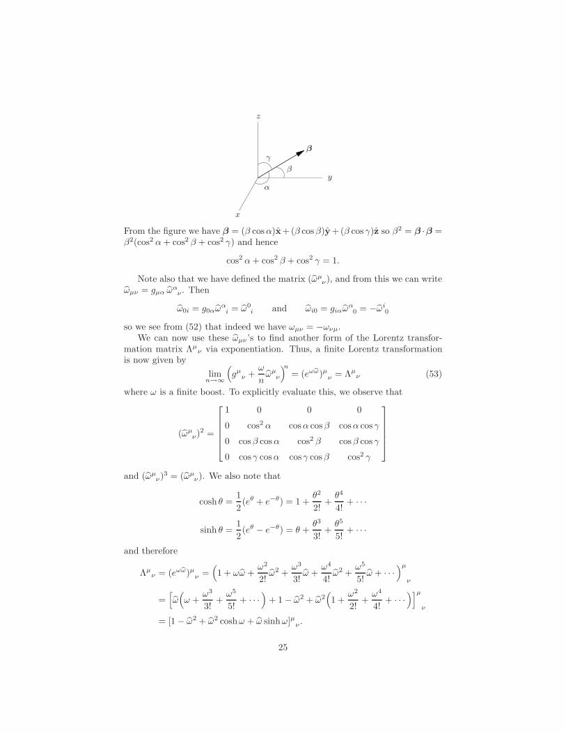
are the direction cosines of the infinitesimal boost β = ω/n. (See the figure be-low.)
24
x
y
z
α
β
γβ
From the figure we have β = (β cosα)x+(β cosβ)y+(β cos γ)z so β2 = β ·β =β2(cos2 α+ cos2 β + cos2 γ) and hence
cos2 α+ cos2 β + cos2 γ = 1.
Note also that we have defined the matrix (ωµν), and from this we can write
ωµν = gµα ωα
ν . Then
ω0i = g0αωα
i = ω0i and ωi0 = giαω
α0 = −ωi
0
so we see from (52) that indeed we have ωµν = −ωνµ.We can now use these ωµν ’s to find another form of the Lorentz transfor-
mation matrix Λµν via exponentiation. Thus, a finite Lorentz transformation
is now given by
limn→∞
(gµ
ν +ω
nωµ
ν
)n= (eωbω)µ
ν = Λµν (53)
where ω is a finite boost. To explicitly evaluate this, we observe that
(ωµν)2 =
1 0 0 0
0 cos2 α cosα cosβ cosα cos γ
0 cosβ cosα cos2 β cosβ cos γ
0 cos γ cosα cos γ cosβ cos2 γ
and (ωµν)3 = (ωµ
ν). We also note that
cosh θ =1
2(eθ + e−θ) = 1 +
θ2
2!+θ4
4!+ · · ·
sinh θ =1
2(eθ − e−θ) = θ +
θ3
3!+θ5
5!+ · · ·
and therefore
Λµν = (eωbω)µ
ν =(1 + ωω +
ω2
2!ω2 +
ω3
3!ω +
ω4
4!ω2 +
ω5
5!ω + · · ·
)µ
ν
=[ω(ω +
ω3
3!+ω5
5!+ · · ·
)+ 1− ω2 + ω2
(1 +
ω2
2!+ω4
4!+ · · ·
)]µν
= [1− ω2 + ω2 coshω + ω sinhω]µν .
25

For example, in the particular case of a boost along the x1-axis we havecosα = 1 and cosβ = cos γ = 0 so that
ωµν =
0 −1 0 0−1 0
0 00 0
(ωµ
ν)2 =
11
00
and hence
eωbω =
coshω − sinhω 0 0
− sinhω coshω 0 0
0 0 1 0
0 0 0 1
= (Λµ
ν).
Therefore, looking at the 0 component for example, we have
x′0 = Λ0νx
ν = x0 coshω − x1 sinhω = coshω(x0 − x1 tanhω)
and comparing this with equation (49) shows that
coshω = γ and tanhω = β (54)
which should be familiar from more elementary courses. In other words, ex-ponentiating an infinitesimal Lorentz boost gives back exactly the same trans-formation matrix as we could have written down directly from equation (49),which should have been expected.
Now let us finish computing the spinor transformation matrix S(Λ) definedin equation (48). First, using ωµ
ν as defined in equation (52) we have
ωµνΣµν = gµρ ωρνΣµν
= ω01Σ
01 + ω02Σ
02 + ω03Σ
03 − ω10Σ
10 − ω20Σ
20 − ω30Σ
30.
But Σ0i = −Σi0 = (i/4)[γ0, γi] where the gamma matrices are given in equation(6) so that
Σ0i =i
2
[0 σi
σi 0
]:=
i
2αi.
Now observe that (as we saw above) ωi0 = giµωµ0 = −ωi0 = ω0i = g0µω
µi = ω0
i
(which also follows from the explicit form of equation (52)) and therefore
ωµνΣµν = 2 ω0iΣ
0i = −2(Σ01 cosα+ Σ02 cosβ + Σ03 cos γ)
= −i(α1 cosα+ α2 cosβ + α3 cos γ)
= −iα · β.
Recall that the Pauli matrices obey the relation (using the summation con-vention on repeated indices)
σiσj = δij + iεijkσk
26

which implies(a · σ)(b · σ) = a · b + i(a× b) · σ
so that (σ · β)2 = β · β = 1. Then from
α · β =
[0 σ · β
σ · β 0
]
(remember this is a block matrix) we see that
(α · β)2 =
[1 00 1
].
This then gives us
S(Λ) = e−i2ωbωµνΣµν
= e−1
2ωα·bβ
= I − ω
2α · β +
1
2!
(ω2
)2
(α · β)2 − 1
3!
(ω2
)3
(α · β)3 + · · ·
= I −α · β[ω
2+
1
3!
(ω2
)3
+ · · ·]
+ I
[1
2!
(ω2
)2
+1
4!
(ω2
)4
+ · · ·]
or simply
S(Λ) = I coshω
2− (α · β) sinh
ω
2. (55)
If this looks vaguely familiar to you, it’s because you may recall from aquantum mechanics course that the rotation operator for spin 1/2 particles isgiven by
U(R(θ)) = e−iθ·J/~ = e−iθ·σ/2~ = I cosθ
2− i(σ · θ) sin
θ
2.
Anyway, to put equation (55) into a more useable form, we make note of thefollowing identities:
cosh2 x− sinh2 x = 1
sinh(x+ y) = sinhx cosh y + coshx sinh y
cosh(x+ y) = coshx cosh y + sinhx sinh y
and these then imply
1 + cosh 2x = 2 cosh2 x
cosh 2x− 1 = 2 sinh2 x
coshx
2=
[1
2(1 + coshx)
]1/2
sinhx
2=
[1
2(coshx− 1)
]1/2
.
27

Using equation (54) we then have
coshω
2=
[1
2(1 + γ)
]1/2
and sinhω
2=
[1
2(γ − 1)
]1/2
.
Now we use the relativistic expressions E = γm and p = γmv = Ev so thatp = p/p = p/Ev. Since we want to boost from the rest frame of the particle to
a frame where it has velocity v, we have β = −v and β = −p. We also haveE2/m2 = γ2 = 1/(1− β2) so that
β2 = 1− m2
E2=E2 −m2
E2=
(E +m)(E −m)
E2
orEβ = [(E +m)(E −m)]1/2.
Therefore
(γ + 1
2
)1/2
=
(E/m+ 1
2
)1/2
=
(E +m
2m
)1/2
= coshω
2(56a)
(γ − 1
2
)1/2
=
(E −m
2m
)1/2
= sinhω
2(56b)
−σ · β = +σ · p =σ · pEβ
=σ · p
[(E +m)(E −m)]1/2(56c)
Using equations (56) in equation (55) then yields our desired final form
S(Λ) =
(E +m
2m
)1/2
1 0 pz/(E +m) p−/(E +m)
0 1 p+/(E +m) −pz/(E +m)
pz/(E +m) p−/(E +m) 1 0
p+/(E +m) −pz/(E +m) 0 1
(57)
where p± = px ± ipy.We now use equation (57) to write down the arbitrary momentum free par-
ticle solutions to the Dirac equation. For a particle at rest we have p = 0, sothe Dirac Hamiltonian (equation (2)) becomes simply E = α · p + βm = βm,and the Dirac equation is just
(iγ0∂0 −m)ψ(x) = 0.
Using (in block form)
γ0 =
[1
−1
]
28

we write the equation in the form
i
1
1
−1
−1
∂0
φ1
φ2
χ1
χ2
= m
φ1
φ2
χ1
χ2
.
The obvious solutions are of the form
ψr(x) = wr(0)e−iǫrmt
where
ǫr =
{+1 for r = 1, 2
−1 for r = 3, 4
and
w1(0) =
1000
w2(0) =
0100
w3(0) =
0010
w4(0) =
0001
.
Since mt = p0x0 = pµx
µ is a Lorentz scalar (where ˚ means the rest frame),we may write the phase in the form e−iǫrpµxµ
. And since the spinor part is givenby wr(p) = S(Λ)wr(0), the general solution is thus
ψr(x) = wr(p)e−iǫrpµxµ
= wr(p)e−iǫrp·x (58)
where the rth column of (57) gives wr(p). Recalling that ψψ is a Lorentz scalar,it is also easy to see directly from the columns of (57) that
wr(0)ws(0) = wr(p)ws(p) = ǫrδrs.
But note that we can multiply wr(0) by any constant to fix the normalization.The last topic to cover in this section is to consider what happens under
parity (i.e., space reflection). In this case equation (31) can not be solved byconsidering the infinitesimal transformation (44). Now we have the Lorentztransformation t→ t and x→ −x so the Lorentz matrix ΛP is given by
(ΛP )µν =
1
−1
−1
−1
= gµν
and we seek a matrix denoted by P (rather than S) that satisfies
(ΛP )µνγ
ν = P−1γµP.
29

In particular, γ0 = P−1γ0P and −γi = P−1γiP or −Pγi = γiP . It should beclear that this is satisfied by choosing anything of the form
P = eiϕγ0. (59)
In other words, we have
ψ(x)P−→ ψ′(x′) = ψ′(t,−x) = eiϕγ0ψ(t,x).
5 Easier Approach to the Spinor Solutions
The Dirac equation is (α · p + βm)ψ = Eψ, and with γ0 = β,γ = βα we have(γ ·p+m)ψ = γ0Eψ. Using pµ = (p0 = p0 = E,p) we write the Dirac equationas (γ0p0 − γ · p−m)ψ = (γµpµ −m)ψ = 0 or just
(/p−m)ψ = 0. (60)
(For simplicity we will generally leave out the identity matrix in these equations.)Now note that multiplying {γµ, γν} = 2gµν by scalars aµ, bν we obtain
{/a, /b} = 2 a · b (61)
and hence in particular /p/p = p · p = p2. Operating on equation (60) fromthe left with /p + m yields (p2 −m2)ψ = 0, and using pµ = i∂µ this becomes(−∂µ∂
µ −m2)ψ = 0 or(� +m2)ψ = 0.
In other words, each component of any ψ that satisfies the Dirac equation alsosatisfies the Klein-Gordon equation. This equation has the solutions e±ik·x with−k2 +m2 = 0 so that k2
0 − k2 = m2 or k20 = k2 +m2. We define
ωk := +√
k2 +m2 (62)
so that the solution e−ik·x ∼ e−iωkt is referred to as the positive frequency
solution (since in the Schrodinger theory ψ ∼ e−iEt), and the solution e+ik·x ∼eiωkt is called the negative frequency solution.
Let us write the plane wave solutions to the Dirac equation in the form
ψ(x) ∼ u(k)e−ik·x + v(k)eik·x
where k2 = kµkµ = m2. Then (i/∂ −m)ψ = 0 implies
(+/k −m)u(k)e−ik·x + (−/k −m)v(k)eik·x = 0.
Since the positive and negative frequency solutions are independent (they eachsatisfy the Dirac equation separately) this implies
(/k −m)u(k) = 0 (63a)
(/k +m)v(k) = 0. (63b)
30

Using 㵆 = γ0γµγ0, we take the adjoint of each of these and multiply throughby γ0 to obtain
u(k)(/k −m) = 0 (64a)
v(k)(/k +m) = 0. (64b)
For solutions at rest we have k = 0 (and hence k0 = m) so equations (63)become
(γ0 − 1)u(0) = 0
(γ0 + 1)v(0) = 0.
The first of these is
11−1
−1
u(0) = u(0)
which has solutions of the form
u(0) =
∗∗00
where the *’s stand for an arbitrary entry. Similarly, the second of these hassolutions of the form
v(0) =
00∗∗
.
Since each of these has two independent components, we write the rest framesolutions as
u1(0) =
1000
u2(0) =
0100
v1(0) =
0010
v2(0) =
0001
(65)
up to an arbitrary constant.Using
(/k −m)(/k +m) = k2 −m2 ≡ 0 (66)
along with the fact that u(k) satisfies equation (63a), we see that any spinor ofthe form u′ = (/k +m)u will automatically satisfy (/k −m)u′ = 0. We thereforewrite the solutions for arbitrary k in the form
ur(k) = c(/k +m)ur(0) (67a)
−vr(k) = c′(/k −m)vr(0) (67b)
31

where the normalization constants c and c′ are to be determined, and the (−)sign in front of vr(k) is an arbitrary convention. We must also therefore have(by inserting γ0γ0 = I in front of the m)
u†r(k) = c∗u†r(0)(γ0γµγ0kµ +m) = c∗ur(0)(/k +m)γ0
and−v†r(k) = c′∗v†r(0)(γ0γµγ0kµ −m) = c′∗vr(0)(/k −m)γ0
so that
ur(k) = c∗ur(0)(/k +m) (68a)
−vr(k) = c′∗vr(0)(/k −m). (68b)
Next, from equations (66), (67) and (68) we see that
ur(k)vs(k) = −c∗c′ur(0)(/k +m)(/k −m)vr(0) ≡ 0
and similarlyvr(k)us(k) = 0.
This means that ψψ ∼ uu+ vv, and since u and v are independent solutions, itfollows from the fact that ψψ is Lorentz invariant that uu and vv must also beLorentz invariant. We fix our normalization by requiring that
ur(k)us(k) = ur(0)us(0) = 2mδrs (69a)
vr(k)vs(k) = vr(0)vs(0) = −2mδrs (69b)
where the (−) sign in equation (69b) is due to the form of γ0 and equations(65).
Let us now find the normalization constants in equations (67). We computeusing equations (66), (67) and (68):
ur(k)us(k) = |c|2 ur(0)(/k +m)2us(0) = |c|2 ur(0)(/k2+ 2m/k +m2)us(0)
= |c|2 ur(0)2m(m+ /k)us(0) = 2m |c|2 ur(0)(/k +m)us(0)
= 2m |c|2 u†r(0)γ0(γ0k0 − γ · k +m)us(0).
But
(γ · k)us(0) =
[0 σ · k
−σ · k 0
]
∗∗00
∼
00∗∗
while
ur(0) = u†r(0)γ0 =[∗ ∗ 0 0
] [ 1−1
]∼[∗ ∗ 0 0
]
32

and henceur(0)(γ · k)us(0) ≡ 0.
We also have k0 = E and
γ0us(0) =
11−1
−1
∗∗00
= us(0)
so that (using equation (69))
ur(k)us(k) = 2m |c|2 (E +m)ur(0)us(0) = ur(0)us(0)
which then implies (choosing the phase equal to +1)
c = [2m(E +m)]−1/2 (70)
In an exactly analogous manner, we have
vr(k)vs(k) = |c′|2 vr(0)(/k −m)2vs(0) = |c′|2 vr(0)(/k2 − 2m/k +m2)vs(0)
= |c′|2 vr(0)(2m2 − 2mEγ0 − 2mγ · k)vs(0).
But
vr(0)(γ · k)vs(0) =[0 0 ∗ ∗
][
1
−1
][0 σ · k
−σ · k 0
]
00∗∗
=[0 0 ∗ ∗
]
∗∗00
≡ 0
and
vr(0)γ0vs(0) = vr(0)
[1−1
] [0∗
]= −vr(0)vs(0).
Therefore
vr(k)vs(k) = |c′|2 2m(m+ E)vr(0)vs(0) = vr(0)vs(0)
so thatc′ = [2m(E +m)]−1/2 = c.
Lastly, observe that equations (69) and the forms (65) require that we mul-tiply each of equations (65) by
√2m. We are then left with our final result
33
ur(k) =1√
E +m(/k +m)
[ϕr
0
](71a)
vr(k) =−1√E +m
(/k −m)
[0
χr
](71b)
where
ϕ1 = χ1 =
[1
0
]and ϕ2 = χ2 =
[0
1
].
Explicitly, these may be written out using
/k +m = γ0E − γ · k +mI =
[E +m −σ · k+σ · k −E +m
]
where
σ · k =
[k3 k−
k+ −k3
]
and
/k −m = γ0E − γ · k−mI =
[E −m −σ · k+σ · k −(E +m)
]
so that
ur(k) =1√
E +m
[E +m −σ · kσ · k −E +m
][ϕr
0
]=
1√E +m
[(E +m)ϕr
(σ · k)ϕr
]
vr(k) =−1√E +m
[E −m −σ · kσ · k −(E +m)
] [0
χr
]=
1√E +m
[(σ · k)χr
(E +m)χr
]
or
u1(k) =1√
E +m
E +m
0
k3
k+
u2(k) =
1√E +m
0
E +m
k−
−k3
(72a)
v1(k) =1√
E +m
k3
k+
E +m
0
v2(k) =
1√E +m
k−
−k3
0
E +m
(72b)
Note that to within the normalization constant 1/√
2m, these agree with equa-tions (57) as they should.
34

Part II – Useful Facts Dealing With the DiracSpinors
6 Energy Projection Operators and Spin Sums
In order to actually calculate scattering cross sections, there are a number ofproperties of the Dirac spinors that will prove very useful. We will work in thenormalization of Section 5:
ur(k) =1√
E +m(/k +m)
[ϕr
0
](73a)
vr(k) =−1√E +m
(/k −m)
[0
χr
](73b)
(these are just equations (71)) where
ϕ1 = χ1 =
[1
0
]and ϕ2 = χ2 =
[0
1
]
andur(k)us(k) = −vr(k)vs(k) = 2mδrs (74)
(these are equations (69)). We also have the basic equations (63) and (64)
(/k −m)u(k) = 0 = (/k +m)v(k) (75a)
u(k)(/k −m) = 0 = v(k)(/k +m) (75b)
As a consequence of these we immediately have the identity
u(k){(/k −m), γµ}us(k) = 0.
Noting that {γµ, γν} = 2gµν implies {/k, γµ} = 2kµ, this last equation can bewritten
ur(k)(2kµ − 2mγµ)us(k) = 2kµur(k)us(k) − 2mur(k)γµus(k) = 0.
Letting µ = 0 and using (74) yields (where k0 = Ek = ωk)
u†r(k)us(k) = 2ωkδrs. (76a)
Similarly,
vr(k){(/k +m), γµ}vs(k) = vr(k)(2kµ + 2mγµ)vs(k) = 0
results inv†r(k)vs(k) = 2ωkδrs. (76b)
35
From equation (10) we see that /k†
= 㵆kµ = γ0γµγ0kµ = γ0/kγ0 so thatfrom equations (73) we have
ur(k)vs(k) =−1
E +m
[ϕ†
r 0](γ0/kγ0 +m)γ0(/k −m)
[0χs
]
=−1
E +m
[ϕ†
r 0]γ0(/k +m)(/k −m)
[0χs
].
There is also a similar result for vr(k)us(k), so that using (/k + m)(/k −m) =k2 −m2 = 0 (equation (66)) we obtain
ur(k)vs(k) = vr(k)us(k) = 0. (77)
For convenience, let us define kµ = (k0,−k) where we still have k20−k2 = m2
or ωk = ω−k = ωek=√
k2 +m2. From equation (75a) we have (/k+m)vs(−k) =0, so multiplying this from the left by ur(k) and also multiplying ur(k)(/k−m) =0 from the right by vs(−k) and then adding, we obtain
0 = ur(k)(/k + /k)vs(−k) = ur(k)(γ0k0 − γiki + γ0k0 + γiki)vs(−k)
= ur(k)2γ0k0vs(−k) = 2ωku†r(k)vs(−k)
so thatu†r(k)vs(−k) = 0 = v†r(k)us(−k) (78)
where we didn’t bother to repeat the identical argument for v†u.Now for the energy projection operators. First note that because of equations
(75) we have /ku = mu and /kv = −mv. Then if we define
Λ±(k) = ±/k +m (79)
we have
Λ+u = /ku+mu = 2mu while Λ+v = /kv +mv = 0 (80a)
and
Λ−u = −/ku+mu = 0 while Λ−v = −/kv +mv = 2mv. (80b)
Similarly we find
uΛ+ = 2mu while vΛ+ = 0 (80c)
and
uΛ− = 0 while vΛ− = 2mv. (80d)
36
It is easy to see that the Λ± are indeed projection operators since
(Λ±)2 = (±/k +m)2 = /k2 ± 2m/k +m2 = 2m(±/k +m) = 2mΛ± (81a)
Λ±Λ∓ = (±/k +m)(∓/k +m) = −/k2+m2 = 0 (81b)
Λ+ + Λ− = 2mI. (81c)
(If we had defined Λ± = (±/k +m)/2m, then these would be (Λ±)2 = Λ± andΛ+ + Λ− = 1 which is the more common way to define projection operators.)
To put Λ± into a more useable form, we proceed as follows. First note thatwe have ur(k) = S(Λ)ur(0) and vr(k) = S(Λ)vr(0). Using S†γ0 = γ0S−1 (equa-tion (40)) these yield ur(k) = u†r(0)S†γ0 = ur(0)S−1 and vr(k) = vr(0)S−1. Itwill be convenient for us to change notation slightly and write u(k, r) = ur(k)so that uα(k, r) represents the αth spinor component of u(k, r). Then considerthe sum
2∑
r=1
[uα(k, r)uβ(k, r) − vα(k, r)vβ(k, r)]
= Sαµ
{2∑
r=1
[uµ(0, r)uν(0, r)− vµ(0, r)vν(0, r)]
}S−1
νβ . (82)
Observe that what we might call the outer product of a column vector a witha row vector bT is
a1
...an
[b1 · · · bn
]=
a1b1 · · · a1bn
......
anb1 · · · anbn
so that (abT )ij = aibj . (This is just the usual rule for multiplying matrices. Itis also just the usual direct product of two matrices.) To evaluate the term inbraces on the right-hand side of equation (82), we first note that from equations(73) we have
u(0, r) =√
2m
[ϕr
0
]and v(0, r) =
√2m
[0
χr
]
and hence the sum of outer products is given by (note γ0 changes the sign of χin v)
u(0, 1)u(0, 1) + u(0, 2)u(0, 2)− v(0, 1)v(0, 1)− v(0, 2)v(0, 2)
= 2m
1 0 0 00 0 0 00 0 0 00 0 0 0
+
0 0 0 00 1 0 00 0 0 00 0 0 0
37
+
0 0 0 00 0 0 00 0 1 00 0 0 0
+
0 0 0 00 0 0 00 0 0 00 0 0 1
= 2mI.
Then the term in braces in equation (82) is just 2mδµν and we have
2∑
r=1
[uα(k, r)uβ(k, r) − vα(k, r)vβ(k, r)] = 2mδαβ .
Taking the (α, β)th element of equation (81c) this last equation can be writtenas
2∑
r=1
[uα(k, r)uβ(k, r) − vα(k, r)vβ(k, r)] = Λ+αβ + Λ−
αβ.
Multiplying from the right by Λ+βµ and using equations (80) and (81) we have
2∑
r=1
[uα(k, r)2muµ(k, r) − 0] = 2mΛ+αµ + 0
or our desired result
2∑
r=1
uα(k, r)uβ(k, r) = Λ+αβ = (/k +m)αβ . (83a)
Similarly, multiplying by Λ−βµ yields
−2∑
r=1
vα(k, r) vβ(k, r) = Λ−αβ = (−/k +m)αβ . (83b)
Another way to see this is to use the explicit expressions from the end ofSection 5:
/k +m =
[E +m −σ · k+σ · k −E +m
]and /k −m =
[E −m −σ · k+σ · k −(E +m)
]
together with
ur(k) =√E +m
[ϕr
σ·kE+mϕr
]and vr(k) =
√E +m
[σ·k
E+mχr
χr
]
so we also have
ur(k) = u†r(k)γ0 =√E +m
[ϕ†
r −ϕ†r
σ·kE+m
]
vr(k) = v†r(k)γ0 =√E +m
[χ†
rσ·k
E+m −χ†r
].
38
We now use these to form the outer products
ur(k)ur(k) = (E +m)
ϕrϕ†r −ϕrϕ
†r
σ·kE+m
σ·kE+mϕrϕ
†r − σ·k
E+mϕrϕ†r
σ·kE+m
vr(k)vr(k) = (E +m)
σ·kE+mχrχ
†r
σ·kE+m − σ·k
E+mχrχ†r
χrχ†r
σ·kE+m −χrχ
†r
Noting that
χ1χ†1 + χ2χ
†2 =
[1
0
][1 0
]+
[0
1
][0 1
]=
[1 0
0 1
]
with a similar result for ϕ1ϕ†1 + ϕ2ϕ
†2, we have
2∑
r=1
ur(k)ur(k) = (E +m)
1 − σ·k
E+m
σ·kE+m − (σ·k)2
(E+m)2
2∑
r=1
vr(k)vr(k) = (E +m)
[(σ·k)2
(E+m)2 − σ·kE+m
σ·kE+m −1
].
But (σ · k)2 = k2 = E2 −m2 = (E +m)(E −m) and we are left with
2∑
r=1
ur(k)ur(k) =
[E +m −σ · kσ · k −E +m
]= /k +m = Λ+(k)
2∑
r=1
vr(k)vr(k) =
[E −m −σ · kσ · k −(E +m)
]= /k −m = Λ−(k)
which agree with equations (83).
7 Trace Theorems
We now turn to the various trace theorems and some related algebra. Everythingis based on the relation
{γµ, γν} = 2gµν (84)
where
gµν =
1−1
−1−1
.
39

We also use the matrix γ5 defined by (see equation (42))
γ5 = γ5 := iγ0γ1γ2γ3 =i
4!εαβµνγ
αγβγµγν . (85)
As we saw before, that the last expression is equivalent to iγ0γ1γ2γ3 is an imme-diate consequence of the fact that both εαβµν and γαγβγµγν are antisymmetricin all indices which must also be distinct. Then there are 4! possible orders ofindices, and putting them into increasing order introduces the same sign fromboth terms. This is just a special case of the general result that for any twoantisymmetric tensors Ai1··· ir
and T j1··· jr we have
Ai1··· irT i1··· ir = r!A|i1··· ir |T
i1··· ir
where |i1 · · · ir| means to sum over all sets of indices with i1 < i2 < · · · < ir.Now note that
{γ5, γµ} = 0 (86)
becauseγ5γ
µ = iγ0γ1γ2γ3γµ = −iγµγ0γ1γ2γ3 = −γµγ5
due to the fact that no matter what µ is, γµ will anticommute with preciselythree of the γ’s in γ5, and hence gives an overall (−) sign. We also have
(γ5)2 = 1. (87)
To see this, first recall that equation (84) implies (γ0)2 = +1 and (γi)2 = −1.Then
(γ5)2 = −γ0γ1γ2γ3γ0γ1γ2γ3 = +γ0γ0γ1γ2γ3γ1γ2γ3 = γ1γ2γ3γ1γ2γ3
= γ1γ1γ2γ3γ2γ3 = −γ2γ3γ2γ3 = +γ2γ2γ3γ3 = (−1)2 = 1.
In what follows, we shall leave off the identity matrix so as to not clutterthe equations. For example, to say γµγ
µ = 4 really means γµγµ = 4I.
Theorem 3. The gamma matrices have the following properties:
γµγµ = 4 (88a)
γµ/aγµ = −2/a (88b)
γµ/a/bγµ = 4a · b (88c)
γµ/a/b/cγµ = −2/c/b/a (88d)
γµ/a/b/c/dγµ = 2(/d/a/b/c + /c/b/a/d) (88e)
{/a, /b} = 2a · b (88f)
40

Proof. Since (γ0)2 = 1 and (γi)2 = −1, we have
γµγµ = (γ0)2 + γiγ
i = (γ0)2 −∑
(γi)2 = 1− 3(−1) = 4.
Next we have (using (88a))
γµ/aγµ = aνγµγ
νγµ = aν(−γνγµ + 2gνµ)γµ = −/aγµγ
µ + 2/a = −2/a.
Note that (88f) simply follows by multiplying {γµ, γν} = 2gµν by aµbν . Then
γµ/a/bγµ = γµ/abν(−γµγν + 2gµν) = −γµ/aγ
µ/b + 2/b/a
= +2/a/b + 2/b/a by (88b)
= 4a · b by (88f).
Now observe that
{γµ, /a} = aν{γµ, γν} = aν2gµν = 2aµ.
Then
γµ/a/b/cγµ = γµ/a/b(−γµ/c + 2cµ) = −γµ/a/bγ
µ/c + 2/c/a/b
= −4a · b/c + 2/c/a/b by (88c)
= −4a · b/c + 2/c(−/b/a+ 2a · b) by (88f)
= −2/c/b/a.
Finally, we have
γµ/a/b/c/dγµ = γµ/a/b/c(−γµ/d+ 2dµ) = −γµ/a/b/cγ
µ/d+ 2/d/a/b/c
= 2(/c/b/a/d+ /d/a/b/c) by (88d). vTheorem 4. The gamma matrices obey the following trace relations:
tr I = 4 (89a)
tr γ5 = 0 (89b)
tr(odd no. γ’s) = 0 (89c)
tr /a/b = 4a · b (89d)
tr /a/b/c/d = 4[(a · b)(c · d) + (a · d)(b · c)− (a · c)(b · d)] (89e)
tr γ5/a = 0 (89f)
41
tr γ5/a/b = 0 (89g)
tr γ5/a/b/c = 0 (89h)
tr γ5/a/b/c/d = −4iεµνρσaµbνcρdσ = +4iεµνρσaµbνcρdσ (89i)
tr /a1 · · · /a2n = tr /a2n · · · /a1 (89j)
Proof. That tr I = 4 is obvious. Next,
−i trγ5 = tr γ0γ1γ2γ3 = − tr γ1γ2γ3γ0 by (84)
= + tr γ1γ2γ3γ0 by the cyclic property of the trace
Therefore tr γ5 = 0. Now let n be odd and use the fact that (γ5)2 = 1 to write
tr γ1 · · ·γn = tr γ1 · · · γnγ5γ5
= − tr γ5γ1 · · ·γnγ5 by (86) with n odd
= − tr γ1 · · ·γn(γ5)2 by the cyclic property of the trace
= − tr γ1 · · ·γn
so that tr γ1 · · · γn = 0. Next we have
tr /a/b =1
2(tr /a/b + tr /b/a) =
1
2tr(/a/b + /b/a)
=1
2(2a · b) tr I = 4a · b by (88f) and (89a).
For the next identity we compute
tr /a/b/c/d = − tr /b/a/c/d+ 2a · b tr /c/d
= + tr /b/c/a/d− 2a · c tr /b/d+ 8(a · b)(c · d)
= − tr /b/c/d/a+ 2a · d tr /b/c − 8(a · c)(b · d) + 8(a · b)(c · d)
= − tr /a/b/c/d+ 8(a · d)(b · c)− 8(a · c)(b · d) + 8(a · b)(c · d)
where the first line follows from (88f), the second and third from (88f) and (89d),and the last by the cyclic property of the trace. Hence
tr /a/b/c/d = 4[(a · d)(b · c)− (a · c)(b · d) + (a · b)(c · d)].
Equation (89f) follows from (89c) or from tr γ5/a = − tr /aγ5 = − tr γ5/a = 0 wherewe used (86) and the cyclic property of the trace.
For the next result, note that tr γ5/a/b = aµbν tr γ5γµγν . If µ = ν then
tr γ5(γµ)2 = ± tr γ5 = 0 by (89b). Now assume that µ 6= ν. Then
γ5γµγν = iγ0γ1γ2γ3γµγν = ±iγαγβ
42

where α 6= β are those two indices (out of 0, 1, 2, 3) remaining after moving γµγν
through to obtain (γµ)2 and (γν)2 (each equal to ±1). But
tr γαγβ = − tr γβγα = − tr γαγβ = 0
if α 6= β (by (84) and the cyclic property of the trace). Therefore tr γ5γµγν = 0.
Continuing, we see that (89h) follows from (89c). Now consider tr γ5γµγνγργσ.
If any two indices are the same, then this is zero since we just showed thattr γ5γ
µγν = 0. Thus assume that µ 6= ν 6= ρ 6= σ, i.e., (µ, ν, ρ, σ) is a permuta-tion of (0, 1, 2, 3). If we choose (µ, ν, ρ, σ) = (0, 1, 2, 3) then we have
tr γ5γ0γ1γ2γ3 = −i tr(γ5)
2 = −4i = −4iε0123.
Since both sides of this equation are totally antisymmetric, it must hold for allvalues of the indices so that
tr γ5γµγνγργσ = −4iεµνρσ
and hencetr γ5/a/b/c/d = −4iεµνρσaµbνcρdσ.
For the second part of (89i), note that εµνρσ is not a tensor by definition.Indeed, we have ε0123 := ε0123 := +1. But the only non-vanishing terms inεµνρσaµbνcρdσ comes when all the indices are distinct, and a0 = a0 while ai =−ai etc., so we actually have
εµνρσaµbνcρdσ = −εµνρσaµbνcρdσ.
Finally, let us define γµ = −(γµ)T . Then {γµ, γν} = 2gµν , and hence byTheorem 2 there exists a matrix C such that CγµC−1 = −(γµ)T . Then we have
tr /a1 · · · /a2n = trC/a1 · · · /a2nC−1 = trC/aC−1C/a2 · · ·C/a2nC
−1
= (−1)2n tr /aT1 · · · /a
T2n = tr(/a2n · · · /a1)
T
= tr /a2n · · · /a1. v
43

Part III – Group Theoretic Approach
8 Decomposing the Lorentz Group
In this part we will derive the Dirac equation from the standpoint of represen-tations of the Lorentz group. To begin with, let us first show that the (homoge-neous) Lorentz transformations form a group. (By “homogeneous” we mean asdistinct from the general Poincare (or inhomogeneous Lorentz) transformationsof the form x′µ = Λµ
νxν + aµ where aν is a constant.)
Clearly the set of all Lorentz transformations contains the identity trans-formation (i.e., zero boost), and corresponding to each Lorentz transformationΛµ
ν there is an inverse transformation Λ−1 = ΛT (equation (28)). Thus we needonly show that the set of Lorentz transformations is closed, i.e., that the com-position of two Lorentz transformations is another such transformation. Well,if x′µ = Λµ
αxα and x′′ν = Λ′ν
βx′β , then
x′′ν = Λ′νβx
′β = Λ′νβΛβ
αxα
and therefore (using equation (30))
x′′νx′′ν = Λ′νβΛβ
αxαΛ′
νρΛρσxσ = (Λ′ν
βΛ′νρ)(Λ
βαΛρσ)xαxσ
= gβρ(Λβ
αΛρσ)xαxσ = ΛραΛρσxαxσ = gσαx
αxσ = xσxσ
and therefore the composition of two Lorentz transformations is also a Lorentztransformation (because it preserves the length xσxσ). This defines the Lorentz
group.If we let xµ denote the “lab frame” and x′µ the “moving frame,” then for a
pure boost along the x1-axis we have (note that this is just equation (49) withβ → −β and switching the primes)
x0 = γ(x′0 + βx′1) x1 = γ(x′1 + βx′0) x2 = x′2 x3 = x′3
with the corresponding Lorentz transformation matrix
Λ(β)µν =
γ γβ
γβ γ
1
1
. (90)
However, we can also include purely spatial rotations since these also preservethe lengths x · x and hence also xµxµ = (x0)2 − x · x. For example, a purelyspatial rotation about the x3-axis has the Lorentz transformation matrix
Λ(θ)µν =
1
cos θ − sin θ
sin θ cos θ
1
. (91)
44
Since such rotations clearly form a group themselves, the spatial rotations forma subgroup of the Lorentz group. However, the set of pure boosts does notform a subgroup. In fact, the commutator of two different boost generators is arotation generator (see equation (93b) below), and this is the origin of Thomasprecession.
It is easy to see that the Lorentz group depends on six real parameters.From a physical viewpoint, there can be three independent boost directions,so there will be three boost parameters (like the direction cosines in equation(52)), and there are obviously three independent rotation angles for anotherthree parameters (for example, the three Euler angles). Alternatively, Lorentztransformations are also defined by the condition ΛT gΛ = g. Since both sidesof this equation are symmetric 4 × 4 matrices, there are (42 − 4)/2 + 4 = 10constraint equations coupled with the 16 entries in a 4× 4 matrix for a total of6 independent entries.
For an infinitesimal boost β ≪ 1, equation (90) becomes
Λ(β)µν =
1 β
β 1
1
1
:= I + ω10M
10
where I = (gµν) = (δµ
ν ), the infinitesimal boost parameter along the x-axis isdefined by ω10 := β, and we define the generator of boosts along the x-axis by
M10 =
0 11 0
00
.
Let us define ω01 := −ω10 and M01 := −M10 so that
ω10M10 =
1
2(ω10M
10 + ω10M10) =
1
2(ω10M
10 + ω01M01).
Since we can clearly do the same thing for boosts along the x2 and x3 directions,we see that the general boost generator matrix (as in equation (52)) is given by
1
2(ωi0M
i0 + ω0iM0i)
where
M20 =
0 10
1 00
and M30 =
0 10
01 0
.
45

Similarly, for an infinitesimal spatial rotation θ ≪ 1, equation (91) becomes
Λ(θ)µν =
1
1 −θθ 1
1
:= I + ω12M
12
where now the parameter for rotation about the x3-axis is defined by ω12 := θ,and the corresponding rotation generator is defined by
M12 =
0
0 −1
1 0
0
.
Again, we define ω21 = −ω12 and M21 = −M12 so that
ω12M12 =
1
2(ω12M
12 + ω12M12) =
1
2(ω12M
12 + ω21M21).
With
M23 =
0
0
0 −1
1 0
and M31 =
0
0 1
0
−1 0
as the generators of rotations about the x1 and x2 axes respectively, we havethe spatial rotation generator matrix
1
2(ωijM
ij + ωjiMji).
(Notice that the signs appear wrong in M31, but they’re not. This is becauseall rotations are defined by the right-handed orientation of R3 as shown in thefigure below.)
x
x
x
y
y
y
z
z
z
Just as we did in equation (53), the matrix representing a finite Lorentztransformation (including both boosts and rotations) is obtained by exponen-tiating the infinitesimal results so that we have the general result (where wedefine ω00 = ωii = 0)
Λ = e1
2ωµνMµν
. (92)
46

Let us define the vectors
M = (M23,M31,M12) and N = (M10,M20,M30).
By direct computation you can easily show that (using the summation conven-tion on repeated letters)
[Mi,Mj ] = εijkMk (93a)
[Ni, Nj ] = −εijkMk (93b)
[Mi, Nj ] = εijkNk. (93c)
Note that these are now to be interpreted as the components of vectors in R3
where the metric is just δij . In other words, they are a shorthand for relationssuch as [M23,M31] = M12 plus its cyclic permutations. They are exactly thesame as you have seen in elementary treatments of angular momentum in quan-tum mechanics. It is also worth observing that from equation (93b) we see thata combination of two boosts in different directions results in a rotation ratherthan another boost. As mentioned above, this is in fact the origin of Thomasprecession.
However, we see that the vectors M and N don’t commute, and hence wedefine the new vectors
J =i
2(M + iN) and K =
i
2(M− iN)
so thatM = −i(J + K) and N = K− J. (94)
Now you can also easily show that
[Ji, Jj ] = iεijkJk (95a)
[Ki,Kj ] = iεijkKk (95b)
[Ji,Kj ] = 0 (95c)
which are simply the commutation relations for two sets of independent, com-muting angular momentum generators of the group SU(2). Thus we have shownthat a general Lorentz transformation is of the equivalent forms
Λ = eωi0Mi0+ 1
2ωijMij
= ea·N+b·M = e−(a+ib)·J+(a−ib)·K. (96)
And since J and K commute, this is
Λ = e−(a+ib)·Je(a−ib)·K. (97)
Note that since M and N are real and antisymmetric, it is easy to see thatJ† = K so that Λ† = ΛT = Λ−1 which again shows that Lorentz transformationsare orthogonal.
47

9 Angular Momentum in Quantum Mechanics
While the decomposition (97) may look different, it is actually exactly the sameas what you have probably learned in quantum mechanics when you studiedthe addition of angular momentum. So, to help clarify what we have done, let’sbriefly review the theory of representations of the rotation group as applied toangular momentum in quantum mechanics.
First, let’s take a brief look at how the spatial rotation operator is defined.If we rotate a vector x in R3, then we obtain a new vector x′ = R(θ)x whereR(θ) is the matrix that represents the rotation. In two dimensions this is
[x′
y′
]=
[cos θ − sin θsin θ cos θ
] [xy
].
If we have a scalar wavefunction ψ(x), then under rotation we obtain a newwavefunction ψR(x′), where ψ(x) = ψR(x′) = ψR(R(θ)x). (See the figurebelow.)
x
x′
θψ(x)
ψR(x′)
Alternatively, we can write
ψR(x) = ψ(R−1(θ)x).
Since R is an orthogonal transformation (it preserves the length of x) we knowthat R−1(θ) = RT (θ), and in the case where θ ≪ 1 we then have
R−1(θ)x =
[x+ θy−θx+ y
].
Expanding ψ(R−1(θ)x) with these values for x and y we have
ψR(x) = ψ(x+ θy, y − θx) = ψ(x)− θ[x∂y − y∂x]ψ(x)
or, using pi = −i∂i this is
ψR(x) = ψ(x)− iθ[xpy − ypx]ψ(x) = [1− iθLz]ψ(x).
For finite θ we exponentiate this to write ψR(x) = e−iθLzψ(x), and in the caseof an arbitrary angle θ in R3 this becomes
ψR(x) = e−iθ·Lψ(x).
48

In an abstract notation we write this as
|ψR〉 = U(R)|ψ〉
where U(R) = e−iθ·L. For simplicity and clarity, we have written U(R) ratherthan the more complete U(R(θ)) which we continue to do unless the morecomplete notation is needed.
What we just did was for orbital angular momentum. In the case of spin thereis no classical counterpart, so we define the spin angular momentum operatorS to obey the usual commutation relations, and the spin states to transformunder the rotation operator e−iθ·S. It is common to use the symbol J to standfor any type of angular momentum operator, for example L,S or L+S, and thisis what we shall do from now on. The operator J is called the total angular
momentum operator. (This example applied to a scalar wavefunction ψ,which represents a spinless particle. Particles with spin are described by vectorwavefunctions ψ (as we have seen for the Dirac spinors), and in this case thespin operator S serves to mix up the components of ψ under rotations.)
The angular momentum operators J2 = J · J and Jz commute and hencehave the simultaneous eigenstates denoted by |jm〉 with the property that (with~ = 1)
J2|jm〉 = j(j + 1)|jm〉 and Jz|jm〉 = m|jm〉where m takes the 2j + 1 values −j ≤ m ≤ j. Since the rotation operator isgiven by U(R) = e−iθ·J we see that [U(R), J2] = 0. Then
J2U(R)|jm〉 = U(R)J2|jm〉 = j(j + 1)U(R)|jm〉
so that the magnitude of the angular momentum can’t change under rotations.However, [U(R), Jz] 6= 0 so the rotated state will no longer be an eigenstate ofJz with the same eigenvalue m.
Note that acting to the right we have the matrix element
〈j′m′|J2U(R)|jm〉 = 〈j′m′|U(R)J2|jm〉 = j(j + 1)〈j′m′|U(R)|jm〉
while acting to the left gives
〈j′m′|J2U(R)|jm〉 = j′(j′ + 1)〈j′m′|U(R)|jm〉
and therefore〈j′m′|U(R)|jm〉 = 0 unless j = j′. (98)
We also make note of the fact that acting with J2 and Jz in both directionsyields
〈j′m′|J2|jm〉 = j′(j′ + 1)〈j′m′|jm〉 = j(j + 1)〈j′m′|jm〉and
〈jm′|Jz |jm〉 = m′〈jm′|jm〉 = m〈jm′|jm〉so that (as you should have already known)
〈j′m′|jm〉 = δj′jδm′m. (99)
49

In other words, the states |jm〉 form a complete orthonormal set, and the stateU(R)|jm〉 must be of the form
U(R)|jm〉 =∑
m′
|jm′〉〈jm′|U(R)|jm〉 =∑
m′
|jm′〉D(j)m′m(θ) (100)
whereD
(j)m′m(θ) := 〈jm′|U(R)|jm〉 = 〈jm′|e−iθ·J|jm〉. (101)
(Notice the order of susbscripts in the sum in equation (100). This is the same asthe usual definition of the matrix representation [T ]e = (aij) of a linear operatorT : V → V defined by Tei =
∑j ejaji.)
Since for each j there are 2j + 1 values of m, we have constructed a (2j +1)× (2j+1) matrix D(j)(θ) for each value of j. This matrix is referred to as thejth irreducible representation of the rotation group. The word “irreducible”means that there is no subset of the space of states {|jj〉, |j,m− 1〉, . . . , |j,−j〉}that transforms into itself under all rotations U(R(θ)). Put in another way, arepresentation is irreducible if the vector space on which it acts has no invariantsubspaces.
Now, it is a general result of the theory of group representations that anyrepresentation of a finite group or compact Lie group is equivalent to a unitaryrepresentation, and any reducible unitary representation is completely reducible.Therefore, any representation of a finite group or compact Lie group is eitheralready irreducible or else it is completely reducible (i.e., the space on which theoperators act can be put into block diagonal form where each block correspondsto an invariant subspace). However, at this point we don’t want to get into thegeneral theory of representations, so let us prove directly that the representa-tions D(j)(θ) of the rotation group are irreducible. Recall that the raising andlowering operators J± are defined by
J±|jm〉 = (Jx ± iJy)|jm〉 =√j(j + 1)−m(m± 1) |j,m± 1〉.
In particular, the operators J± don’t change the value of j when acting on thestates |jm〉.
Theorem 5. The representations D(j)(θ) of the rotation group are irreducible.In other words, there is no subspace of the space of states |jm〉 (for fixed j) thattransforms among itself under all rotations.
Proof. Fix j and let V be the space spanned by the 2j+ 1 vectors |jm〉 := |m〉.We claim that V is irreducible with respect to rotations U(R). This meansthat given any |u〉 ∈ V , the set of all vectors of the form U(R)|u〉 (i.e., for allrotations U(R)) spans V . (Otherwise, if there exists |v〉 such that {U(R)|v〉}didn’t span V , then V would be reducible since the collection of all such U(R)|v〉would define an invariant subspace.)
50

To show V is irreducible, let V = span{U(R)|u〉} where |u〉 ∈ V is arbitrarybut fixed. For infinitesimal θ we have U(R(θ)) = e−iθ·J = 1 − iθ · J and inparticular U(R(εx)) = 1− iεJx and U(R(εy)) = 1− iεJy. Then
J±|u〉 = (Jx ± iJy)|u〉 =
{1
iε[1− U(R(εx))]± i
(1
iε[1− U(R(εy))]
)}|u〉
=1
ε
{± [1− U(R(εy))]− i+ iU(R(εx))
}|u〉 ∈ V
by definition of V and vector spaces. Since J± acting on |u〉 is a linear combi-
nation of rotations acting on |u〉 and this is in V , we see that (J±)2 acting on|u〉 is again some other linear combination of rotations acting on |u〉 and hence
is also in V . So in general, we see that (J±)n|u〉 is again in V .By definition of V , we may write (since j is fixed)
|u〉 =∑
m
|jm〉〈jm|u〉 =∑
m
|m〉〈m|u〉
= |m〉〈m|u〉+ |m+ 1〉〈m+ 1|u〉+ · · ·+ |j〉〈j|u〉
where m is simply the smallest value of m for which 〈m|u〉 6= 0 (and not allof the terms up to 〈j|u〉 are necessarily nonzero). Acting on this with J+ weobtain (leaving off the constant factors and noting that J+|j〉 = 0)
J+|u〉 ∼ |m+ 1〉〈m|u〉+ |m+ 2〉〈m+ 1|u〉+ · · ·+ |j〉〈j − 1|u〉 ∈ V .
Since 〈m|u〉 6= 0 by assumption, it follows that |m+ 1〉 ∈ V .We can continue to act on |u〉 with J+ a total of j−m times at which point
we will have shown that |m+ j −m〉 = |j〉 := |jj〉 ∈ V . Now we can apply J−2j + 1 times to |jj〉 to conclude that the 2j + 1 vectors |jm〉 all belong to V ,
and thus V = V . (This is because we have really just applied the combinationof rotations (J−)2j+1(J+)j−m to |u〉, and each step along the way is just some
vector in V .) vNow suppose that we have two angular momenta J1 and J2 with [J1,J2] = 0.
Then J12, J2
2, J1z and J2z all commute, and hence we can construct simultane-ous eigenstates which we write as |j1j1m1m2〉. Furthermore, with J = J1 + J2
it follows that J2, Jz , J12 and J2
2 all commute, and hence we can also con-struct the simultaneous eigenstates |j1j2jm〉. However, J2 does not commutewith either J1z or J2z , so if we specify J2, then we are only free to also specifyJz = J1z + J2z and not J1z or J2z individually.
Since j1 and j2 are fixed, there are 2j1 +1 possible values for m1, and 2j2 +1possible values of m2 for a total of (2j1 +1)(2j2 +1) linearly independent statesof the form |j1j2m1m2〉, which must be the same as the number of states of theform |j1j2jm〉. The maximum possible value of m = m1 +m2 is j1 + j2. Butthe next value j1 + j2− 1 can be due to either m1 = j1 and m2 = j2− 1, or dueto m1 = j1 − 1 and m2 = j2. And as we go to lower values of m, there will be
51

even more possible choices. Since the largest m value is j1 + j2, there must be astate of total j = j1 + j2, and a multiplet of 2(j1 + j2) + 1 states correspondingto this value of j. But this j = j1 + j2 state only accounts for one of the stateswith m = j1 + j2−1, and hence there must be another state with j = j1 + j2−1and its corresponding multiplet of 2(j1 + j2 − 1) + 1 states |j1j2jm〉.
We can continue to consider states with lower and lower j values and corre-sponding multiplets of 2j + 1 possible m values. However, the total number ofstates must equal (2j1 + 1)(2j2 + 1), and hence we have the relation
j1+j1∑
j=N
2j + 1 = (2j1 + 1)(2j2 + 1)
where N is to be determined. Using the formula (which you can check)
n2∑
j=n1
j =1
2(n2 − n1 + 1)(n2 + n1)
it takes a little bit of elementary algebra to show that N2 = (j1 − j2)2 and
therefore the minimum value of j is |j1 − j2|, i.e., |j1 − j2| ≤ j ≤ j1 + j2.What else can we say about the angular momentum states |j1j2m1m2〉?
These are really direct product states and are written in the equivalent forms
|j1j2m1m2〉 = |j1m1〉 ⊗ |j2m2〉 = |j1m1〉|j2m2〉.
(Remark: You may recall from linear algebra that given two vector spaces Vand V ′, we may define a bilinear map V × V ′ → V ⊗ V ′ that takes orderedpairs (v, v′) ∈ V × V ′ and gives a new vector denoted by v ⊗ v′. Since thismap is bilinear by definition, if we have the linear combinations v =
∑xivi
and v′ =∑yjv
′j then v ⊗ v′ =
∑xiyj(vi ⊗ v′j). In particular, if V has basis
{ei} and V ′ has basis {e′j}, then {ei ⊗ e′j} is a basis for V ⊗ V ′ which is thenof dimension (dimV )(dim V ′) and called the direct (or tensor) product ofV and V ′. Then, if we are given two operators A ∈ L(V ) and B ∈ L(V ′),the direct product of A and B is the operator A ⊗ B defined on V ⊗ V ′ by(A⊗B)(v ⊗ v′) := A(v)⊗B(v′).)
When we write 〈j1j2m1m2|j′1j′2m′1m
′2〉 we really mean
(〈j1m1| ⊗ 〈j2m2|)(|j′1m′1〉 ⊗ |j′2m′
2〉) = 〈j1m1|j′1m′1〉〈j2m2|j′2m′
2〉
so that by equation (99) we have
〈j1j2m1m2|j′1j′2m′1m
′2〉 = δj1j′
1δj2j′
2δm1m′
1δm2m′
2(102)
We point out that a special case of this result is
〈j1j2m1m2|j1j2m′1m
′2〉 = δm1m′
1δm2m′
2
As we will see below, the matrix elements 〈j1j2jm|j1j2m1m2〉 will be veryimportant to us. Now consider the expression Jz = J1z+J2z. What the operator
52

on the right really stands for is J1z ⊗ I + I ⊗ J2z . Then on the one hand wehave
〈j1j2jm|Jz|j1j2m1m2〉 = 〈j1j2jm|(J1z ⊗ I + I ⊗ J2z)(|j1m1〉 ⊗ |j2m2〉)
= 〈j1j2jm|(J1z |j1m1〉 ⊗ |j2m2〉+ |j1m1〉 ⊗ J2z|j2m2〉)
= (m1 +m2)〈j1j2jm|(|j1m1〉 ⊗ |j2m2〉)
= (m1 +m2)〈j1j2jm|j1j2m1m2〉
while acting to the left with Jz we have
〈j1j2jm|Jz|j1j2m1m2〉 = m〈j1j2jm|j1j2m1m2〉.
Comparing these last two results shows that
〈j1j2jm|j1j2m1m2〉 = 0 unless m = m1 +m2. (103)
We also see that for i = 1, 2 we can let Ji2 act either to the right or left also
and we have
〈j′1j′2jm|Ji2|j1j2m1m2〉 = ji(ji + 1)〈j′1j′2jm|j1j2m1m2〉
= j′i(j′i + 1)〈j′1j′2jm|j1j2m1m2〉
so that〈j′1j′2jm|j1j2m1m2〉 = 0 unless j′1 = j1 and j′2 = j2. (104)
In a similar manner, by letting the operator act to both the right and left wecan consider the matrix elements of J1
2, J22, J2 and Jz to show that (compare
with equation (102))
〈j′1j′2j′m′|j1j2jm〉 = δj′1j1δj′2j2δj′jδm′m (105)
Since both of the sets {|j1j2m1m2〉} and {|j1j2jm〉} are complete (i.e., theyform a basis for the two particle angular momentum states where j1 and j2 arefixed), we can write either set as a function of the other:
|j1j2jm〉 =∑
m1,m2
(m1+m2=m)
|j1j2m1m2〉〈j1j2m1m2|j1j2jm〉 (106)
or|j1j2m1m2〉 =
∑
j(m=m1+m2)
|j1j2jm〉〈j1j2jm|j1j2m1m2〉. (107)
The matrix elements 〈j1j2jm|j1j2m1m2〉 are called Clebsch-Gordan coeffi-
cients, and may always be taken to be real (see below). Note that the Clebsch-Gordan coefficients are nothing more than the matrix elements of the transitionmatrix that changes between the |j1j2jm〉 basis and the |j1j2m1m2〉 basis. In
53

fact, since both bases are orthonormal, the Clebsch-Gordan coefficients define aunitary transformation matrix.
That the Clebsch-Gordan coefficients may be taken as real is the so-called“Condon-Shortley convention.” It follows from the fact that the maximumvalues of j and m are jmax = j1 + j2 = mmax so that (leaving out the fixed j1and j2 labels of the two particles so as not to be too confusing)
|jmaxmmax〉 =∑
m1+m2=mmax
|m1m2〉〈m1m2|jmaxmmax〉
= |j1j2〉〈j1j2|jmaxmmax〉.
But then
〈jmaxmmax|jmaxmmax〉 = 〈jmaxmmax|j1j2〉〈j1j2|j1j2〉〈j1j2|jmaxmmax〉
or (since 〈jm|jm〉 = 〈m1m2|m1m2〉 = 1)
1 = |〈jmaxmmax|j1j2〉|2 .
Therefore we take as our (Condon-Shortley) convention 〈jmaxmmax|j1j2〉 := +1,and this forces the rest of the Clebsch-Gordan coefficients to be real also sincethey are constructed by repeated application of the operator J− = J1− + J2−
to the |jm〉 and |m1m2〉 states starting at the top.Let us see what we can say about the rotation operator that acts on com-
posite angular momentum states. The corresponding rotation operator is
e−iθ·J = e−iθ·J1 ⊗ e−iθ·J2 = e−iθ·J1e−iθ·J2
where the last equality is just a commonly used shorthand notation. Writingthe rotation operator as the direct product U(R) = U1(R) ⊗ U2(R), its actionis defined by
[U1(R)⊗ U2(R)]|j1j2m1m2〉 = [U1(R)⊗ U2(R)](|j1m1〉 ⊗ |j2m2〉)= U1(R)|j1m1〉 ⊗ U2(R)|j2m2〉.
Applying equation (100) we can now write
[U1(R)⊗ U2(R)]|j1j2m1m2〉 = U1(R)|j1m1〉 ⊗ U2(R)|j2m2〉
=∑
m′1m′
2
|j1m′1〉 ⊗ |j2m′
2〉D(j1)m′
1m1
(θ)D(j2)m′
2m2
(θ)
=∑
m′1m′
2
|j1j2m′1m
′2〉D
(j1)m′
1m1
(θ)D(j2)m′
2m2
(θ) (108)
which implies
〈j1j2m′1m
′2|U1(R)⊗ U2(R)|j1j2m1m2〉 = D
(j1)m′
1m1
(θ)D(j2)m′
2m2
(θ). (109)
54
We regard the left side of this equation as the m′1m
′2,m1m2 matrix element of a
[(2j1 +1)(2j2 +1)× (2j1 +1)(2j2 +1)]-dimensional matrix called the direct (orKronecker) product of D(j1)(θ) and D(j2)(θ) and written D(j1)(θ)⊗D(j2)(θ).In other words
[D(j1)(θ)⊗D(j2)(θ)]m′
1m′
2,m1m2
= D(j1)m′
1m1
(θ)D(j2)m′
2m2
(θ).
The double subscripts make the direct product of two matrices look confusing,but the result really isn’t if we just use the definitions carefully. So to understandthis, we need to take another small linear algebra detour.
If we have a vector space V with basis {e1, . . . , en} and another space V ′
with basis {e′1, . . . , e′m}, then we have the space V ⊗V ′ with the basis {ei⊗ e′j}which we take to have the ordering
{e1 ⊗ e′1, e1 ⊗ e′2, . . . , e1 ⊗ e′m, e2 ⊗ e′1, . . . , e2 ⊗ e′m, . . . , en ⊗ e′1, . . . , en ⊗ e′m}.
Given the operators A ∈ L(V ) and B ∈ L(V ′), the matrix representations of Aand B are defined by Aei =
∑k ekaki and Be′j =
∑l e
′lblj , and thus the matrix
representation of A⊗B is also defined in the same way by
(A⊗B)(ei ⊗ e′j) = Aei ⊗Be′j =∑
kl
(ek ⊗ e′l)akiblj =∑
kl
(ek ⊗ e′l)(A⊗B)kl,ij .
But Aei is just the ith column of the matrix (aij), and now we have each rowand column labeled by a double subscript so that, e.g., the (1, 1)th column ofthe matrix representation of A⊗B is given relative to the above ordered basisby
(A⊗B)(e1 ⊗ e′1)
=∑
kl
(ek ⊗ e′l)ak1bl1
= {a11b11, a11b21, . . . , a11bm1, a21b11, . . . , a21bm1, . . . , an1b11, . . . , an1bm1}
Since this is really a column vector, we see by careful inspection that it is justa11 times the first column of B followed by a21 times the first column of B, andso on down to an1 times the first column of B. And in general, the matrix ofA⊗B is given in block matrix form by
a11B a12B · · · a1nB
......
...
an1B an2B · · · annB
.
There is another basic result from linear algebra that we should review beforetreating U(R). Suppose we have an operator T ∈ L(V ), and let W be aninvariant subspace of V . By this we mean that T (W ) ⊂ W . Let {e1, . . . , em}
55

be a basis for W , and extend this to a basis {e1, . . . , em, em+1, . . . , en} for V .By definition of invariant subspace, for any 1 ≤ i ≤ m the effect of T on ei isgiven by
Tei =
m∑
j=1
ejaji 1 ≤ i ≤ m
for appropriate scalars aji. Compare this to
Tei =m∑
j=1
ejbji +n∑
j=m+1
ejcji m+ 1 ≤ i ≤ n
for some scalars bji and cji where we have assumed that the subspace spannedby {em+1, . . . , en} is not an invariant subspace itself. Since the ith column of[T ] = (aij) is given by Tei, a moments thought should convince you that thematrix representation for T will be of the block matrix form
[A B0 C
].
If it turns out that {em+1, . . . , en} also spans an invariant subspace W ′, thenfor m + 1 ≤ i ≤ n we will have Tei =
∑nj=m+1 ejcji and the representation of
T will look like [A 00 C
].
In this case we have V = W ⊕W ′ (the direct sum) and we write T = TW ⊕TW ′
where TW is the restriction of T to W and TW ′ is the restriction of T to W ′.(As a reminder, we say that V is the direct sum of subspaces W1, . . . ,Wr
if the union of bases for the Wi is a basis for V , and in this case we writeV = W1 ⊕ · · · ⊕Wr . If each of these Wi is also an invariant subspace withrespect to some operator T , then we write T = TW1
⊕ · · · ⊕ TWrand its matrix
representation with respect to this basis will be block diagonal.)Now let’s go back to the rotation operator U(R) = U1(R) ⊗ U2(R). When
we say that a representation is reducible, we mean there exists a basis for thestate space relative to which the matrix representation of all relevant operatorsis block diagonal. We now want to show that the set of direct product matricesis reducible, and thus in the |j1j2jm〉 basis the matrix representation of thedirect product takes the form
. . .
56
where each block represents the (2j+1)× (2j+1) matrix D(j)(θ) for each valueof j = j1 + j2, j1 + j2 − 1, . . . , |j1 − j2|. Symbolically we write this as
D(j1)(θ)⊗D
(j2)(θ) = D(j1+j2)(θ)⊕D
(j1+j2−1)(θ)⊕ · · · ⊕D|j1−j2|(θ) (110)
The idea here is just a somewhat complicated version of the usual result fromlinear algebra dealing with the matrix representation of a linear operator undera change of basis. So let’s first review that topic.
Given an operator T , its representation A = (aij) := [T ]e on a basis {ei} isdefined by Tei =
∑j ejaji. If we want to change to a new basis {e′i}, then we
first define the transition matrix P by e′i =∑
j ejpji. Then on the one hand wehave the representation A′ = (a′ij) := [T ]e′ given by
Te′i =∑
j
e′ja′ji =
∑
j
∑
k
ekpkja′ji
while on the other hand we have
Te′i = T(∑
j
ejpji
)=∑
j
(Tej)pji =∑
j
∑
k
ekakjpji.
Equating these last two results and using the fact that the {ek} are a basis (andhence linearly independent) we have
∑
j
pkja′ji =
∑
j
akjpji
which in matrix notation is just PA′ = AP . The transition matrix P must benonsingular because either basis can be written in terms of the other, so we areleft with the fundamental result
A′ = P−1AP.
Furthermore, if both bases are orthonormal, then P will be unitary so thatP−1 = P † = P ∗T and we have A′ = P †AP . In terms of components this is
a′ij =∑
kl
p∗ki akl plj . (111)
Now let’s go back and prove equation (110). We first insert complete sets ofthe states |jm〉 into the left side of equation (109) to obtain (again leaving outthe j1 and j2 for neatness)
〈m′1m
′2|U(R)|m1m2〉 =
∑
j′m′
jm
〈m′1m
′2|j′m′〉〈j′m′|U(R)|jm〉〈jm|m1m2〉
=∑
j′m′
jm
〈m′1m
′2|j′m′〉〈m1m2|jm〉D(j)
m′m(θ)δj′j
=∑
j′m′m
〈m′1m
′2|j′m′〉〈m1m2|j′m〉D(j′)
m′m(θ) (112)
57
where the second line follows from equations (98), (101) and the fact that theClebsch-Gordan coefficients are real. From equation (109) we then have (afterrelabeling the dummy index j′ → j)
D(j1)m′
1m1
(θ)D(j2)m′
2m2
(θ) =∑
jm′m
〈m′1m
′2|jm′〉〈m1m2|jm〉D(j)
m′m(θ) (113)
where the sum is over |j1 − j2| ≤ j ≤ j1+j2. Equation (113) is sometimes calledthe Clebsch-Gordan series. Also note that there is no real sum over m′ andm in this equation because we must have m′ = m′
1 +m′2 and m = m1 +m2.
Analogous to the akl in equation (111), we write equation (112) as
〈m′1m
′2|U1(R)⊗ U2(R)|m1m2〉 := Rm′
1m′
2,m1m2
=∑
j′m′m
〈m′1m
′2|j′m′〉〈m1m2|j′m〉D(j′)
m′m(θ).
From equation (106) we have the (real) transition matrix elements which wewrite as
pm1m2,jm = 〈m1m2|jm〉.Defining the analogue of a′ij in equation (111) by
R′j′m′,jm := 〈j′m′|U(R)|jm〉
we then have
〈j′m′|U(R)|jm〉 =∑
m1m2
m′1m′
2
〈m1m2|j′m′〉Rm1m2,m′1m′
2〈m′
1m′2|jm〉
=∑
m1m2
m′1m′
2
∑
j′′m′′m′′
〈m1m2|j′m′〉〈m1m2|j′′m′′〉〈m′1m
′2|j′′m′′〉
×D(j′′)m′′m′′(θ)〈m′
1m′2|jm〉.
But ∑
m1m2
〈j′m′|m1m2〉〈m1m2|j′′m′′〉 = 〈j′m′|j′′m′′〉 = δj′j′′δm′m′′
and ∑
m′1m′
2
〈j′′m′′|m′1m
′2〉〈m′
1m′2|jm〉 = 〈j′′m′′|jm〉 = δj′′jδm′′m
so we are left with
〈j′m′|U(R)|jm〉 =∑
j′′m′′m′′
δj′j′′δm′m′′δj′′jδm′′mD(j′′)m′′m′′(θ) = D
(j)m′m(θ)δj′j
(114)
58

If on the two particle angular momentum space we take our ordered basis{|jm〉} to be
{|j1 + j2, j1+j2〉, |j1 + j2, j1 + j2 − 1〉, . . . , |j1 + j2,−(j1 + j2)〉,|j1 + j2 − 1, j1 + j2 − 1〉, . . . , |j1 + j2 − 1,−(j1 + j2 − 1)〉,. . . , | |j1 − j2| , |j1 − j2|〉, . . . , | |j1 − j2| ,− |j1 − j2|〉}
then equation (114) is just equation (110) in terms of components.Of course, had we just started with U(R) = e−iθ·J and used equations (99)
and (100) we would have again had
〈j′m′|U(R)|jm〉 =∑
m′′
〈j′m′|jm′′〉D(j)m′′m(θ) = D
(j)m′m(θ)δj′j .
But this doesn’t show that in fact the matrix (112) can be put into the blockdiagonal form (110). In other words, the operator e−iθ·J acts on the states |jm〉in a manifestly block diagonal manner (due to equation (100)), whereas theoperator e−iθ·J1 ⊗ e−iθ·J2 acts on the states |m1m2〉 in the complicated mannerof equation (108), and we had to show that this could in fact be put into blockdiagonal form by the appropriate change of basis.
10 Lorentz Invariance and Spin
Before turning to another derivation of the Dirac equation, we need to takea more careful look at the inhomogeneous Lorentz group, also called thePoincare group. These are transformations of the form
xµ = Λµνx
ν + aµ (115)
where we are using the metric
gµν = gµν =
1−1
−1−1
and Λ satisfiesΛT gΛ = g or gµνΛµ
αΛνβ = gαβ. (116)
(This is a consequence of requiring that xµxµ = xνxν where xµ = Λµνx
ν .) Wewill refer to the transformation (115) as simply a “Lorentz transformation,” andsometimes abbreviate it by simply LT. If we compose two successive transfor-mations (115) we obtain
xµ
= Λµ
νxν + aµ
= Λµ
ν(Λναx
α + aν) + aµ
= (Λµ
νΛνα)xα + (Λ
µνa
ν + aµ) (117)
59
which is just another LT, and hence the set of transformations (115) forms agroup called the “Poincare group” as claimed.
From ΛT gΛ = g we see that (detΛ)2 = 1 so that detΛ = ±1. Since theidentity transformation has determinant equal to +1, we restrict ourselves tothe case detΛ = +1 because we will want to look at transformations that differinfinitesimally from the identity transformation. It also follows from equation(116) that gµνΛµ
0Λν0 = 1 or (Λ0
0)2 = 1 +
∑i(Λ
i0)
2 ≥ 1 so that
Λ00 ≥ 1 or Λ0
0 ≤ −1.
Since only the case Λ00 ≥ 1 can be used for an infinitesimal transformation,
we will restrict ourselves from now on to the set of proper, orthochronous
Lorentz transformations. However, note that the set of all Lorentz transfor-mations can be divided into four classes given by detΛ = ±1 and either Λ0
0 ≥ 1or Λ0
0 ≤ −1.Our goal is to relate this to quantum mechanics and the description of quan-
tum mechanical states, so to each transformation (115) we shall associate a uni-tary operator on the (infinite-dimensional) Hilbert space of all physical statevectors, denoted by U(a,Λ). The effect of this operator is defined by
U(a,Λ)ψ(x) := ψ(Λx+ a).
From equation (115) we have
U(a,Λ) = U(a, 1)U(0,Λ) := U(a)U(Λ). (118)
Then using equation (117) we have the multiplication law
U(a′,Λ′)U(a,Λ) = U(Λ′a+ a′,Λ′Λ) (119)
and therefore, in particular
U(a′)U(a) = U(a′ + a) (120a)
U(Λ′)U(Λ) = U(Λ′Λ). (120b)
For an infinitesimal transformation
Λµν = gµ
ν + ωµν (121)
we have from equation (116)
gαβ = (gµα + ωµ
α)(gνβ + ων
β)gµν = (gµα + ωµ
α)(gµβ + ωµβ)
= gαβ + ωβα + ωαβ
and thereforeωαβ = −ωβα.
60

Then we write our operators in the form
U(a) = eiaµP µ
(122a)
U(Λ) = ei2ωµνMµν
(122b)
where the generators Pµ and Mµν remain to be specified. (This is just expo-nentiating the general form of an infinitesimal transformation. Note also thatwe have included a factor of i in the definition of U(Λ) (as compared to equation(92)) because we are now talking about quantum mechanical operators.)
Before proceeding, let us define just what is meant when we say that anoperator transforms as a vector. Recall from linear algebra (yet again) thatunder a rotation R : v → v′ we have Rv = R(viei) = viRei = vie′jR
ji. But
Rv = v′ = v′je′j so that v′j = Rjiv
i defines how the components of a vectortransform. In quantum mechanics we require that the expectation values of anoperator transform in the same way. Thus, if |ψ〉 → |ψ′〉 = U(R)|ψ〉 where U(R)is the unitary quantum mechanical operator corresponding to the rotation R,then an operator A is defined to be a vector operator if
〈ψ′|Ai|ψ′〉 = Rij〈ψ|Aj |ψ〉.
Using |ψ′〉 = U(R)|ψ〉 and the fact that |ψ〉 is arbitary, this yields
U †(R)AiU(R) = RijA
j (123)
where (Rij) is a real, orthogonal matrix that represents rotations in R3.
If we require that the expectation value of a rotated operator in the originalstate be the same as the expectation value of the original operator in the rotatedstate, then 〈ψ|A′|ψ〉 = 〈ψ′|A|ψ′〉 = 〈ψ|U †(R)AU(R)|ψ〉 so that
A′i = U †(R)AiU(R) = RijA
j
which shows the meaning of equation (123). (This is just the difference betweenactive and passive transformations.) In addition, we can multiply both sidesof equation (123) by (R−1)k
i and sum to write U †(R)(R−1)kiA
iU(R) = Ak sothat (since U † = U−1)
U(R)AkU−1(R) = (R−1)kiA
i (124)
which we take as an equivalent definition of a vector operator.The only difference between this rotational case and our present purposes
is that now we are using a Lorentz transformation Λµν instead of the rotation
matrix Rij , but otherwise everything is exactly the same since Λ is also an
orthogonal transformation. (In fact, this is the same as we saw earlier withequation (31) describing why the Dirac gamma matrices are said to transformas vectors.)
(It should be pointed out that what we have done is not the same aschanging between “pictures” such as the Schrodinger and Heisenberg repre-sentations. In that case, we require that the expectation value of an oper-ator in the Schrodinger picture in a Schrodinger state be the same as the
61

expectation value of a Heisenberg operator in a Heisenberg state. In otherwords, 〈ψS |AS |ψS〉 := 〈ψH |AH |ψH〉, and if |ψH〉 = U(t)|ψS〉(= e+iEt|ψS〉),then 〈ψH |AH |ψH〉 = 〈ψS |U †(t)AHU(t)|ψS〉 so that AH = U(t)ASU
†(t). Notethat the U(t) and U †(t) are reversed from what they are in equation (123).)
Another point that we should discuss is the commutation relation betweenvector operators and the generator of rotations, i.e., the angular momentumoperators. These will serve to help classify certain operators. So, recall fromclassical mechanics that a vector v undergoing a rotation dθ changes by anamount dv as shown in the figure below.
α
dθ
dv
v
v + dv
We have ‖dv‖ = ‖v‖ sinα ‖dθ‖ in the direction shown (i.e., perpendicular tothe plane defined by v and dθ) so that dv = dθ × v and v→ v + dv.
But we just saw above that under a rotation R we have vi → Rijv
j so that(using (dθ × v)i = εijkdθjvk and then relabeling)
vi → v′i = Rijv
j = vi + dvi = vi + εijkdθjvk = (δij + εikjdθk)vj
which shows that to first order we have (where in this case there is no differencebetween upper and lower indices since in R3 with cartesian coordinates we havegij = δij anyway)
Rij = δi
j − εijkdθ
k. (125)
Next, expand the left side of (123) to first order using U(R) = e−idθ·J to yield
(1 + idθ · J)Ai(1 − idθ · J) = Ai − idθj [Ai, Jj ].
Finally, using equation (125) in (123) we obtain [Ai, Jj ] = iεijkAk which we canwrite as
[J i, Aj ] = iεijkAk. (126)
This then is the commutation relation of a vector operator with the generatorof angular momentum.
Now back to where we were. To define the Poincare algebra, we need toobtain the commutation relations for the generators. Since [A,B] = 0 implieseAeB = eA+B, we see from equations (120a) and (122a) that
[Pµ, P ν ] = 0. (127)
Now put equation (118) into (119) and use (120b):
U(a′)U(Λ′)U(a)U(Λ) = U(a′)U(Λ′a)U(Λ′)U(Λ)
62
so thatU(Λ′)U(a)U−1(Λ′) = U(Λ′a)
or (dropping the prime on Λ)
U(Λ)eiaµP µ
U−1(Λ) = eiΛµνaνP µ
.
To first order this is
U(Λ)(1 + iaµPµ)U−1(Λ) = 1 + iP νΛν
µaµ
and henceU(Λ)PµU−1(Λ) = P νΛν
µ = (Λ−1)µνP
ν (128)
so that comparison with equation (124) shows that the operator Pµ transformsas a 4-vector.
An equivalent way of writing equation (128) is
U−1(Λ)PµU(Λ) = ΛµνP
ν . (129)
It is worth pointing out the physical meaning of this equation. Suppose we havean eigenstate of Pµ:
Pµ|Ψp〉 = pµ|Ψp〉.Then acting on |Ψp〉 with U(Λ) results in a state with eigenvalue p′µ = Λµ
νpν
because
Pµ[U(Λ)|Ψp〉] = U(Λ)[U−1(Λ)PµU(Λ)]|Ψp〉 = U(Λ)[Λµνp
ν ]|Ψp〉= Λµ
νpν [U(Λ)|Ψp〉]. (130)
In other words, U(Λ) boosts a state with eigenvalue p to a state with eigenvalueΛp. Alternatively, we can say that the expectation value of the operator Pµ inthe boosted state is the same as the expectation value of the boosted operatorΛP in the original state.
Next we want to find the commutation relations for the generators Mµν .Using equation (122b) for infinitesimal ωµν together with equation (121) in(128) we have
(1 +i
2ωµνM
µν)Pα(1− i
2ωρσM
ρσ) = (gαβ − ωα
β)P β
or
(1 +i
2ωµνM
µν)(Pα − i
2ωρσP
αMρσ) = Pα − ωαβP
β
so that (to first order as usual)
Pα − i
2ωµνP
αMµν +i
2ωµνM
µνPα = Pα − ωαβP
β = Pα − gαµωµνPν
= Pα − 1
2ωµν(gαµP ν − gανPµ)
63

where in the last line we antisymmetrized over the indices µ and ν. CancelingPα and equating the coefficients of ωµν (which is just some arbitrary number)we are left with
[Mµν , Pα] = −i(Pµgνα − P νgµα). (131)
It will be important to us later to realize that this result applies to any 4-vector, and not just Pµ. This is because equation (128) applies to any 4-vectorby definition.
Since ωµν is antisymmetric, we may just as well assume that Mµν is too, solet us define the quantities (essentially the same as we did in Section 8)
Ki = Mi0 and Ji =1
2εijkM
jk. (132)
In order to find the commutation relations for the Ji and Ki, we need those forthe Mµν . To obtain these, we perform the following manipulations.
First note that
U(Λ)U−1(Λ) = 1 = U(ΛΛ−1) = U(Λ)U(Λ−1)
and thereforeU−1(Λ) = U(Λ−1).
(This is really just a special case of the general result from group theory thatif ϕ : G → G′ is a homomorphism of groups, then for any g ∈ G we havee′ = ϕ(e) = ϕ(gg−1) = ϕ(g)ϕ(g−1) so that ϕ(g)−1 = ϕ(g−1). In this case, theoperator U(Λ) is the image of the group element Λ under the homomorphismU : Λ → U(Λ). We are also writing U−1(Λ) rather than the more correctU(Λ)−1, but this is common practice.) Next we have
U(Λ)U(Λ′)U−1(Λ) = U(ΛΛ′Λ−1)
which we want to evaluate for infinitesimal transformations. In a symbolicnotation, if we have Λ′ = 1 + ω′ so that ΛΛ′Λ−1 = 1 + Λω′Λ−1 := 1 + ω, then
ωµν = Λµαω′
αβ(Λ−1)βν = (Λ−1)α
µ(Λ−1)βνω
′αβ .
Therefore
U(ΛΛ′Λ−1) = 1 +i
2ωµνM
µν = 1 +i
2(Λ−1)α
µ(Λ−1)βνω
′αβM
µν . (133)
But
U(Λ)U(Λ′)U−1(Λ) = U(Λ)(1 +i
2ω′
αβMαβ)U−1(Λ)
= 1 +i
2ω′
αβU(Λ)MαβU−1(Λ) (134)
so that equating equations (133) and (134) yields
U(Λ)MαβU−1(Λ) = (Λ−1)αµ(Λ−1)β
νMµν . (135)
64
This equation shows (by definition) thatMµν transforms as a second rank tensoroperator.
Using (Λ−1)αµ = gα
µ − ωαµ in equation (135) we have
(1 +i
2ωµνM
µν)Mαβ(1 − i
2ωµνM
µν) = (gαµ − ωα
µ)(gβν − ωβ
ν)Mµν
which to first order expands to
Mαβ − i
2ωµνM
αβMµν +i
2ωµνM
µνMαβ = Mαβ − ωβνM
αν − ωαµM
µβ
ori
2ωµν [Mµν ,Mαβ] = −Mανωβ
ν −Mνβωαν .
Antisymmetrizing over µ and ν we can write the two terms on the right side ofthis equation as
Mανωβν = Mανωµνg
µβ =1
2ωµν(Mανgµβ −Mαµgνβ)
and
Mνβωαν = Mνβωµνg
µα =1
2ωµν(Mνβgµα −Mµβgνα).
Using these, we finally obtain the commutation relation for the generators Mµν
[Mµν ,Mαβ ] = i(Mανgµβ +Mνβgµα −Mαµgνβ −Mµβgνα). (136)
Equations (127), (131) and (136) define the Poincare algebra. An explicitexample of the generators is provided by the matrix Σµν defined in equation(46). You should be able to see the reason for this.
(Technically, one says that these generators define the Lie algebra of thePoincare group, so let me briefly explain what is going on. The Poincare (orinhomogeneous Lorentz) group consists of translations (in four directions), ro-tations (with three degrees of freedom) and boosts (in three directions), each ofwhich is specified by some set of parameters. In other words, we can think ofeach group element as a point in a (in this case) 10-dimensional space. To eachpoint in this space we associate an operator U(a,Λ) = U(a)U(Λ) and hence amatrix. We expand these operators in a neighborhood of the identity, and aseach group parameter is varied, a curve is traced out in the differentiable man-ifold that defines the group space. The derivative of this coordinate curve withrespect to its parameter is the tangent vector to the curve at that point. Thegenerators are then the tangent vectors to each coordinate curve at the identity,and the vector space spanned by the generators is the Lie algebra (which isthen the tangent space at the identity). (In general, an algebra is a vectorspace on which we have also defined the vector product of two vectors. In thiscase, the product is the commutator (or Lie bracket).) In other words, thegenerators are a basis for the tangent space at the identity (the Lie algebra). Itcan be shown that by exponentiating the Lie algebra, one can construct every
65

group element (i.e., the operators U(a,Λ)) at least in a neighborhood of theidentity. The question of whether or not we can get to every group element byexponentiating the Lie algebra is a nontrivial one, and the answer depends onthe topology of the group in question.)
At last we are ready to find the commutation relations for the generators J
and K. Remember that now we are doing this calculation in R3 with the metricgij = δij as discussed following equations (93). Furthermore, εijk is just thepermutation symbol so it doesn’t carry spacetime (tensor) indices. Then using
εijkεklm = δl
iδmj − δm
i δlj
or the equivalent form
εijkεklm = δliδmj − δmiδlj
we have
[Ji, Jj ] =1
4εilmεjrs[M
lm,M rs]
=i
4εilmεjrs(M
rmgsl +Mmsglr −M rlgsm −M lsgmr)
= i εilmεjrsMrmgsl = i εilmεjrlM
rm
= −i εjrlεlimMrm = −i(δjiδrm − δjmδri)M
rm
= iM ij
where M rmδrm = M rr = 0 since M rm is antisymmetric. But we can invert theequation
Ji =1
2εijkM
jk
to write
εlmiJi =1
2εlmiεijkM
jk =1
2(δljδmk − δlkδmj)M
jk =1
2(M lm −Mml) = M lm
and therefore
[Ji, Jj ] = iεijkJk. (137a)
Similarly, we find
[Ji,Kj ] = iεijkKk (137b)
[Ki,Kj ] = −iεijkJk (137c)
It should be clear that J generates rotations and K generates boosts. It isalso important to note that comparing equations (137b) and (126) we see thatK is a polar (or true) vector, whereas J is an axial (or pseudo) vector. This is
66
because letting J → −J, the left side of (137a) does not change sign, whereasthe right side does. This is also a consequence of the fact that J is essentiallythe angular momentum operator r × p which, because of the cross product,depends on the chosen orientation of the coordinate system for its definition.Indeed, under the parity operation x → −x, the boost generators M i0 definedin Section 8 will change sign because we would have β → −β, but the spatialrotation generators M ij will not change sign. (This is essentially because undera rotation dθ we have dv = dθ× v and this doesn’t change sign if both dθ andv change sign.)
Now let’s write out the term
ωµνMµν = 2ω0iM
0i + ωijMij = −2ω0iKi + ωijεijkJk
so that we may write
U(Λ) = ei2ωµνMµν
= e−ia·J+ib·K. (138)
Define
A =1
2(J + iK) and B =
1
2(J− iK) (139)
or, equivalently,
J = A + B and K = −i(A−B). (140)
The reason for this is that now A and B satisfy the simple commutation relations
[Ai, Aj ] = iεijkAk (141a)
[Bi, Bj ] = iεijkBk (141b)
[Ai, Bj ] = 0 (141c)
so they are commuting angular momentum generators. (These are just what wehad in equations (95).)
Using equation (140) in (138) we have (by (141c) also)
U(Λ) = eA·(b−ia)e−B·(b+ia) (142)
and we have (again) decomposed our Lorentz transformation into a product oftwo rotations, i.e., a direct product. It is also worth pointing out that the U(Λ)of equation (142) is unitary if and only if b = 0, i.e., only for a rotation.
Because of equations (141), the generators A and B are represented by(2A + 1)- and (2B + 1)-dimensional angular momentum matrices respectively.Treating A and B as independent variables, we then describe a particle of spinJ = A + B. We thus define the [(2A + 1) × (2B + 1)]-dimensional irreduciblerepresentation (A,B) for any integer values of 2A and 2B by
〈a′b′|A|ab〉 = δb′bJ(A)a′a and 〈a′b′|B|ab〉 = δa′aJ
(B)b′b (143)
67

where a = −A, . . . , A, b = −B, . . . , B and the states are really |ab〉 = |a〉 ⊗ |b〉.The operators are really A⊗ I and I ⊗B so that J
(A)a′a = 〈a′|A|a〉 and similarly
for B. In other words, the operators J(j) are the usual (2j + 1)-dimensionalrepresentation of the rotation group, i.e.,
〈jσ′|Jz |jσ〉 = δσ′σσ
and〈jσ′|J±|jσ〉 =
√j(j + 1)− σ(σ ± 1)δσ′,σ±1.
Although the representation (A,B) is in general reducible, as shown previouslyit is reducible for rotations alone. In other words, it is the product of (2A+ 1)-and (2B + 1)-dimensional representations.
Now note that under space inversion (i.e., parity) we have J → +J (it’s anaxial vector), while K→ −K (it’s a polar vector). But then under space inver-sion we have A→ B and B→ A so the representation (A,B)→ (B,A). There-fore, if we want to construct a wave function that has space-innversion sym-metry, it must transform under a representation of the form (j, j) or, we mustdouble the number of components and have them transform under (j, 0)⊕(0, j).The representations are often denoted by D(A,B)(Λ). The (j, 0) representationcorresponds to A = J and B = 0, and the (2j + 1)-dimensional matrix repre-senting a finite Lorentz transformation we be denoted by D(j)(Λ). Similarly, the(0, j) representation corresponds to A = 0 and B = J and will be denoted by
D(j)
(Λ). From equation (142) we see that the two representations are relatedby
D(j)(Λ) = D(j)
(Λ−1)†. (144)
Let us now see how to describe the action of a Lorentz transformation onthe states. Using equations (127) and (131) it is easy to verify that the operator
M2 = PµP
µ (145)
commutes with all of the generators. (You will find it very helpful to use thegeneral identity [ab, c] = a[b, c] + [a, c]b.) We may thus classify the irreduciblerepresentations of the group by the value of this invariant operator. Since thePµ all commute, they may be simultaneously diagonalized, and hence we definethe states |p〉 such that
Pµ|p〉 = pµ|p〉.To interpret this, let’s look at translations as they are described in the
Schrodinger theory. If we consider a displacement x → x′ = x + a, thenψ(x) → ψ′(x′) = ψ′(x + a) or ψ′(x) = ψ(x − a). Expanding the infinitesi-mal case with ‖a‖ ≪ 1 we have
ψ′(x) = ψ(x− a) = ψ(x) − a ·∇ψ(x) = [1− ia ·P]ψ(x)
where P = −i∇ is the momentum operator. For a finite displacement weexponentiate as usual to write
ψ′(x) = e−ia·Pψ(x).
68
Now, the effect of U(a) (which generates translations by definition) actingon a state |p〉 is given by
U(a)|p〉 = eiaµP µ |p〉 = eiaµpµ |p〉 = eia·p|p〉
so that comparing this with the Schrodinger theory, we identify Pµ as the 4-momentum of the system. It is now clear that equation (145) represents thesquare of the system’s mass.
Until further notice, all of what follows is based on the assumption that weare dealing with particles of nonzero rest mass.
From experience, we know that one-particle states are also characterized bytheir spin, i.e., the angular momentum in the rest frame of the particle. We nowseek the invariant operator that describes spin. Such an operator is
Wσ := −1
2εµνρσM
µνP ρ (146)
which is called the Pauli-Lubanski spin vector. (We will discuss the represen-tations of the Lorentz group in more detail below, and provide some motivationfor this definition when we define the little group.) Note that for a system at restwe have P = 0 and hence Wσ = −(1/2)εµν0σM
µνP 0. Therefore, for a systemat rest we have W0 = 0 and Wi = −(1/2)εµν0iM
µνP 0 = −(1/2)ε0iµνMµνP 0 =
−(1/2)εijkMjkP 0 so that from equation (132) we see that Wi = −mJi. We
also clearly haveWσP
σ = 0 (147)
and from equation (131) it also follows that
[Wσ , Pµ] = 0. (148)
Since Wσ is a 4-vector by construction, it must also have the same commu-tation relation with Mµν that Pσ does (see the comment immediately followingequation (131)), and hence
[Mµν ,Wσ] = −i(Wµgνσ −Wνgµσ). (149)
Then equations (148) and (149) may be used to easily prove
[Wα,Wβ ] = iεαβµνWµP ν (150)
and[Mµν ,WσW
σ] = 0. (151)
Thus, like M 2 = PµPµ, equations (148) and (151) show that S 2 = WσW
σ
commutes with all of the generators. These two invariants are called Casimir
operators, and they are the only such operators for the Poincare group. (Itis a nontrivial theorem that the number of Casimir operators of a Lie group isequal to the rank of the group.)
We now have two operators which may be used to label the irreduciblerepresentations. To find the eigenvalues of WσW
σ we go to the rest frame. Let
69

L(p) be the Lorentz transformation which takes the 4-vector (m,0) to pµ. If|Ψp〉 is the state vector for a system with 4-momentum pµ, then this system atrest is obtained by operating on |Ψp〉 with U(L−1(p)), i.e.,
|Ψrest〉 = U(L−1(p))|Ψp〉.
Then we have
WσWσ|Ψrest〉 = WσW
σU(L−1(p))|Ψp〉 = U(L−1(p))W ′σW
′σ|Ψp〉 (152)
where the operator in the rest frame is given by
W ′σ = U(L(p))WσU
−1(L(p))
and we used the fact that U(L−1(p)) = U−1(L(p)). Since Wσ is a 4-vector, weuse equation (128) to conclude that
W ′σ = (L−1(p))σ
ρWρ
orW ′σ = (L−1(p))σ
ρWρ.
It is also easy to show directly that W ′σW
′σ = WσWσ. Indeed, we have
W ′σW
′σ = (L−1(p))σα(L−1(p))σ
βWαWβ = L(p)α
σ(L−1)σβWαW
β = WαWα
or alternatively
W ′σW
′σ = U(L(p))WσU−1(L(p))U(L(p))W σU−1(L(p))
= U(L(p))WσWσU−1(L(p))
= WσWσ
because S 2 = WσWσ commutes with all of the generators, and hence with any
U(a,Λ).It is also worth noting that (since U(L(p)) is unitary)
〈Ψrest|WσWσ|Ψrest〉 = 〈Ψp|U(L(p))WσW
σU−1(L(p))|Ψp〉 = 〈Ψp|WσWσ|Ψp〉
and therefore we have the equivalent expectation values
〈Ψrest|W ′σW
′σ|Ψrest〉 = 〈Ψrest|WσWσ|Ψrest〉 = 〈Ψp|WσW
σ|Ψp〉= 〈Ψp|W ′
σW′σ|Ψp〉.
The reason for pointing this out is that while they are all mathematically equiv-alent, we will show below that the operator W ′
σW′σ is just −m2S2 which we
think of as measuring the spin of the particle. Since spin is just the angularmomentum in the rest frame, the comments following equation (123) suggestthat from an intuitive viewpoint we want to consider the expectation value〈Ψrest|WσW
σ|Ψrest〉 = 〈Ψp|W ′σW
′σ|Ψp〉.
70
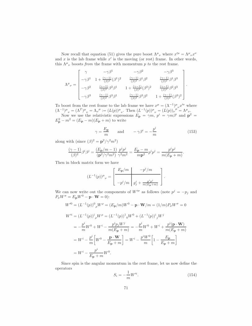
Now recall that equation (51) gives the pure boost Λµν where x′µ = Λµ
νxν
and x is the lab frame while x′ is the moving (or rest) frame. In other words,this Λµ
ν boosts from the frame with momentum p to the rest frame.
Λµν =
γ −γβ1 −γβ2 −γβ3
−γβ1 1 + (γ−1)(β)2 (β1)2 (γ−1)
(β)2 β1β2 (γ−1)
(β)2 β1β3
−γβ2 (γ−1)(β)2 β
2β1 1 + (γ−1)(β)2 (β2)2 (γ−1)
(β)2 β2β3
−γβ3 (γ−1)(β)2 β
3β1 (γ−1)(β)2 β
3β2 1 + (γ−1)(β)2 (β3)2
.
To boost from the rest frame to the lab frame we have xµ = (Λ−1)µνx
′ν where(Λ−1)µ
ν = (ΛT )µν = Λν
µ := (L(p))µν . Then (L−1(p))µ
ν = (L(p))νµ
= Λµν .
Now we use the relativistic expressions Ep = γm, pi = γmβi and p2 =E2
p −m2 = (Ep −m)(Ep +m) to write
γ =Ep
mand − γβi = −p
i
m(153)
along with (since (β)2 = p2/γ2m2)
(γ − 1)
(β)2βiβj =
(Ep/m− 1)
(p2/γ2m2)
pipj
γ2m2=Ep −mmp2
pipj =pipj
m(Ep +m).
Then in block matrix form we have
(L−1(p))µν =
Ep/m −pi/m
−pi/m gij + pipj
m(Ep+m)
.
We can now write out the components of W ′σ as follows (note pj = −pj andPσW
σ = EpW0 − p ·W = 0):
W ′0 = (L−1(p))0ρWρ = (Ep/m)W 0 − p ·W/m = (1/m)PσW
σ = 0
W ′i = (L−1(p))iρW
ρ = (L−1(p))10W0 + (L−1(p))i
jWj
= −pi
mW 0 +W i − pipjW
j
m(Ep +m)= −p
i
mW 0 +W i +
pi(p ·W)
m(Ep +m)
= W i − pi
m
[W 0 − p ·W
Ep +m
]= W i − piW 0
m
[1− Ep
Ep +m
]
= W i − pi
Ep +mW 0.
Since spin is the angular momentum in the rest frame, let us now define theoperators
Si = − 1
mW ′i. (154)
71
It can be shown, after a lot of algebra (see below for the details), that
[Si, Sj ] = iεijkSk (155)
which is just the usual commutation relation for an angular momentum operatorS where the eigenvalues of S2 are equal to s(s+1) with s = 0, 1
2 , 1,32 , . . . . Since
W ′0 = 0, we now have
W ′σW
′σ = W ′iW
′i = −m2S2
so that (see equation (152))
WσWσ|Ψrest〉 = U(L−1(p))W ′
σW′σ|Ψp〉 = −m2s(s+ 1)U(L−1(p))|Ψp〉
orWσW
σ|Ψrest〉 = −m2s(s+ 1)|Ψrest〉. (156)
In summary, the irreducible representations of the Poincare group are char-acterized by two invariants: mass and spin.
Now let’s go back and prove equation (155). This is equivalent to showingthat
[W ′i ,W
′j ] = −imεijkW
′k
because from the definition of Si we have Si = (−1/m)W ′i = (+1/m)W ′i so
that[W ′
i ,W′j ] = m2[Si, Sj] = m2iεijkSk = −imεijkW
′k.
We start fromW ′
i = Wi −pi
E +mW0
where now pi is a c-number since our states are eigenstates of Pµ, and wherefor simplicity we write E instead of Ep. Then using equations (146), (149) and(147) we have (note that now εµνρσ carries spacetime (tensor) indices becauseof equation (146) where both sides are tensors)
[W ′i ,W
′j ] = [Wi −
pi
E +mW0,Wj −
pj
E +mW0]
= [Wi,Wj ]−pj
E +m[Wi,W0]−
pi
E +m[W0,Wj ]
= −1
2εµν
ρipρ[Mµν ,Wj ] +
1
2
pjpρ
E +mεµν
ρi[Mµν ,W0]
− 1
2
pipρ
E +mεµν
ρj [Mµν ,W0]
=i
2εµν
ρipρ(Wµgνj −Wνgµj)−
i
2
pjpρ
E +mεµν
ρi(Wµgν0 −Wνgµ0)
+i
2
pipρ
E +mεµν
ρj(Wµgν0 −Wνgµ0)
72
=i
2(εµ
jρipρWµ − ε ν
j ρipρWν)
− i
2
pρ
E +m(pjε
µ0ρiWµ − pjε
ν0 ρiWν − piε
µ0ρjWµ + piε
ν0 ρjWν)
= iεµjρip
ρWµ − ipρ
E +m(pjε
µ0ρiWµ − piε
µ0ρjWµ)
= ipρWµ(εµjρi −
pj
E +mεµ0ρi +
pi
E +mεµ0ρj
).
Note that this last line vanishes identically if i = j, so we now assume thati 6= j and expand the sums over µ and ρ, keeping in mind that the ε symbolsrestrict the possible values of the indices. For example, since i 6= j we havepρWµεµjρi = pρW 0ε0jρi + pρW kεkjρi where there is no sum over k because itmust be either 1, 2 or 3 depending on what i and j are. But now summing overρ we really don’t have any choices, so that pρWµεµjρi = pkW 0ε0jki +p
0W kεkj0i
where we stress that there is no sum over the repeated index k.Continuing with this process we have (using the fact that p0 = E and re-
membering that there is no sum over any of the indices i, j, k)
[W ′i ,W
′j ] = ipρW 0ε0jρi + ipρW kεkjρi − i
pρpj
E +m(W jεj0ρi +W kεk0ρi)
+ ipρpi
E +m(W iεi0ρj +W kεk0ρj)
= iε0jkipkW 0 + iEW kεkj0i − i
pj
E +m(W jεj0kip
k +W kεk0jipj)
+ ipi
E +m(W iεi0kjp
k +W kεk0ijpi).
Now use the antisymmetry of ε and note that ε0ijk is exactly the same as εijk
to write
[W ′i ,W
′j ] = iεijk
[W 0pk −W kE
+( 1
E +m
)(W jpjp
k −W kpjpj +W ipipk −W kpipi)
].
Next look at the four terms in parenthesis. By adding and subtracting theadditional term W kpkp
k we can rewrite this term as
(W ipi +W jpj +W kpk)pk −W k(pipi + pjpj + pkpk)
= (Wµpµ −W 0E)pk +W kp2
where we also used∑3
l=1 plpl = −∑plpl = −p2. But Wµpµ = 0, and recalling
that E2 = p2 +m2 we finally have
[W ′i ,W
′j ] = iεijk
[W 0pk −W kE +
( 1
E +m
)(−W 0Epk +W kp2)
]
73
= iεijk
[W 0pk −W k
(E − p2
E +m
)−W 0pk
( E
E +m
)]
= iεijk
[W 0pk −W k
(E2 +mE − p2
E +m
)−W 0pk
( E
E +m
)]
= iεijk
[W 0pk −mW k −W 0pk
( E
E +m
)]
= iεijk
[W 0pk
(1− E
E +m
)−mW k
]
= iεijkm
[W 0pk
E +m−W k
]
= −imεijkW′k
which is what we wanted to show.We still have to motivate the definition (146) of the Pauli-Lubanski spin
vector. This is based on what is called the “method of induced representations”of the inhomogeneous Lorentz group.
Since all of the Pµ commute, we can describe our states as eigenstates of the4-momentum. Let us label these states as |Ψp,σ〉 where σ stands for all otherdegrees of freedom necessary to describe the state. Then by definition we have
Pµ|Ψp,σ〉 = pµ|Ψp,σ〉.
From equation (122a) we see how these states transform under translations:
U(a)|Ψp,σ〉 = eiaµpµ |Ψp,σ〉.
What we now need to figure out is how they transform under homogeneousLorentz transformations U(Λ).
Using equation (129) we see that
Pµ[U(Λ)|Ψp,σ〉] = U(Λ)[U−1(Λ)PµU(Λ)]|Ψp,σ〉 = U(Λ)[ΛµνP
ν ]|Ψp,σ〉= Λµ
νpν [U(Λ)|Ψp,σ〉]
so that the state U(Λ)|Ψp,σ〉 is an eigenstate of Pµ with eigenvalue Λµνp
ν andhence must be some linear combination of the states |ΨΛp,σ〉. Thus we write
U(Λ)|Ψp,σ〉 =∑
σ′
Cσ′σ(Λ, p)|ΨΛp,σ′〉. (157)
We think of the |Ψp,σ〉 as forming a basis for the space carrying a representationof the Poincare group, and therefore in general the matrix Cσ′σ(Λ, p) will becomplicated. However, recall from basic linear algebra that we can diagonalizea matrix by finding suitable linear combinations of the basis vectors (these will
74
then form a basis of eigenvectors) relative to which the matrix is diagonal. Butif any eigenvalue has multiplicity greater than one, then all we can do is put thematrix into block diagonal form where each block is an invariant subspace. Inour present situation, we will assume that by using suitable linear combinationsof the Cσ′σ(Λ, p) it is possible to choose the labels σ so that the matrix Cσ′σ(Λ, p)will be block diagonal, and hence for σ in the appropriate range, each block willform an irreducible representation of the Poincare group. We will identify thestates of a specific type of particle with each of these irreducible representations.
To analyze the structure of the coefficients Cσ′σ(Λ, p) in a particular irre-ducible representation, first note that all proper orthochronous Lorentz trans-formations leave both the quantity pµp
µ and the sign of p0 invariant. Hence foreach value of p2 and each sign of p0, we can choose a “standard” 4-momentumpµ and write any other pµ in this same class as
pµ = Lµν(p)pν (158)
where Lµν(p) is some standard Lorentz transformation that depends both on
pµ and our reference pµ. (The six classes are p2 > 0 and p2 = 0 together witheach sign of p0, along with p2 < 0 and pµ = 0. But only the three classesp2 > 0 with p0 > 0, p2 = 0 with p0 > 0, and pµ = 0 have any known physicalinterpretation.) We then define the states |Ψp,σ〉 by
|Ψp,σ〉 := N(p)U(L(p))|Ψp,σ〉 (159)
where N(p) is a normalization factor to be determined.Observe that p = L(p)p so that Λp = L(Λp)p where Λ is any homogeneous
Lorentz transformation. Then p = L−1(Λp)Λp = L−1(Λp)ΛL(p)p so that thetransformation L−1(Λp)ΛL(p) takes p back to p. This transformation thenbelongs to the subgroup of the homogeneous Lorentz group consisting of thosetransformations Λµ
ν that leave p invariant:
Λµν p
ν = pµ. (160)
This subgroup is called the little group.For example, if we consider the class defined by p2 > 0 and p0 > 0, then
we can take pµ = (m, 0, 0, 0) so that p2 = m2 > 0 and p0 = m > 0. Thenthe little group is just SO(3) (the ordinary group of rotations in R3 with posi-tive determinant) because rotations are the only proper orthochronous Lorentztransformations that leave at rest a particle with p = 0.
For an infinitesimal transformation Λµν = gµ
ν + ωµν we then must have
ωµν p
ν = 0 (161)
and a general expression for ωµν that satisfies this is
ωµν = εµνρσ pρnσ
75

where nσ is an arbitrary 4-vector. The corresponding unitary transformationU(Λ) is then
U(Λ) = 1 +i
2ωµνM
µν = 1 +i
2εµνρσ p
ρnσMµν
orU(Λ) = 1− inσWσ
where
Wσ =1
2εµνρσM
µνP ρ
is the Pauli-Lubanski spin vector. Note that we replaced pρ by P ρ because U(Λ)acts only on the states |Ψp,σ〉. This is the motivation for equation (146) thatwe were looking for.
Since Λp = p, we see from equation (157) that we may write
U(Λ)|Ψp,σ〉 =∑
σ′
Dσ′σ(Λ)|Ψp,σ′〉 (162)
where the Dσ′σ(Λ) form a representation of the little group. Indeed, for anyΛ, Λ′ we have
∑
σ′
Dσ′σ(Λ′Λ)|Ψp,σ′〉 = U(Λ′Λ)|Ψp,σ〉 = U(Λ′)U(Λ)|Ψp,σ〉
= U(Λ′)∑
σ′′
Dσ′′σ(Λ)|Ψp,σ′′〉
=∑
σ′σ′′
Dσ′′σ(Λ)Dσ′σ′′ (Λ′)|Ψp,σ′〉
which shows that
Dσ′σ(Λ′Λ) =∑
σ′′
Dσ′σ′′(Λ′)Dσ′′σ(Λ)
and hence that the Dσ′σ(Λ) are in fact a representation of the little group (i.e., ahomomorphism from the group of all such Λ to the group of matrices Dσ′σ(Λ)).
Acting on equation (159) with an arbitrary U(Λ) we have (by inserting theidentity transformation appropriately)
U(Λ)|Ψp,σ〉 = N(p)U(Λ)U(L(p))|Ψp,σ〉 = N(p)U(ΛL(p))|Ψp,σ〉
= N(p)U(L(Λp))U(L−1(Λp)ΛL(p))|Ψp,σ〉.
Let us define the little group transformation known as the Wigner rotation
W (Λ, p) := L−1(Λp)ΛL(p)
76

(which was the original Λ used as an example to define the little group) so usingequation (162) this last equation becomes
U(Λ)|Ψp,σ〉 = N(p)U(L(Λp))U(W (Λ, p))|Ψp,σ〉
= N(p)∑
σ′
Dσ′σ(W (Λ, p))U(L(Λp))|Ψp,σ′〉
or, using equations (159) and (158)
U(Λ)|Ψp,σ〉 =N(p)
N(Λp)
∑
σ′
Dσ′σ(W (Λ, p))|ΨΛp,σ′〉. (163)
Thus we see that, aside from determining the normalization factors, we havereduced the problem of finding the coefficients Cσ′σ in equation (157) to theproblem of finding the representations of the little group. This is the method
of induced representations. For our present purposes, this is as far as wereally need to go with this.
However, we can take a look at the normalization because it will give us twoimportant basic results that are of great use in quantum field theory. We firstwant to show that when integrating over p “on the mass shell” (meaning thatp2 = m2), the invariant volume element is
d3p
(2π)32ωp
where ωp = +√
p2 +m2. (The numerical factors aren’t necessary for Lorentzinvariance.) To see this, first observe that
d4p
(2π)42πδ(p2 −m2)θ(p0)
is manifestly Lorentz invariant for proper orthochronous Lorentz transforma-tions. (The step function is defined by θ(x) = 1 for x ≥ 0 and θ(x) = 0 forx < 0.) This is because with detΛ = 1 we have d4p′ = |∂p′/∂p|d4p = d4p, andfor timelike pµ an orthochronous transformation can’t change the sign of p0 sothe step function doesn’t change. Then we have
d4p
(2π)42πδ(p2 −m2)θ(p0) =
d4p
(2π)3δ(p2
0 − ω2p)θ(p0)
=d3p dp0
(2π)3δ[(p0 − ωp)(p0 + ωp)]θ(p0)
=d3p dp0
(2π)31
2ωp
[δ(p0 − ωp) + δ(p0 + ωp)]θ(p0)
=d3p dp0
(2π)32ωp
δ(p0 − ωp)
=d3p
(2π)32ωp
77
where the first line is because p2 − m2 = p20 − p2 − m2 = p2
0 − ω2p; the third
line follows because integrating over all p0 gives contributions at both p0 = +ωp
and p0 = −ωp, and using δ(ax) = (1/ |a|)δ(x); the fourth line is because thetheta function restricts the range of integration to p0 > 0 so δ(p0 + ωp) alwaysvanishes; and the last line follows because we want to integrate a function overd3p so integrating over p0 with the delta function just gives 1. This result isreally a shorthand notation for
d3p
(2π)32ωp
=
∫
p0
d4p
(2π)42πδ(p2 −m2)θ(p0). (164)
Another way to see this is to write the integral of an arbitrary functionf(p) = f(p0,p) as
∫d4p δ(p2 −m2)θ(p0)f(p) =
∫d3p dp0 δ(p
20 − p2 −m2)θ(p0)f(p0,p)
=
∫d3p
1
2ωp
δ(p0 − ωp)f(p0,p)
=
∫d3p
2ωp
f(ωp,p)
which also shows that when integrating over the mass shell p2 = m2 the invariantvolume element is d3p/ωp = d3p/
√p2 +m2.
The second result we want to show is that the invariant delta function
(2π)32ωpδ(p − q) is Lorentz invariant (where p2 = q2 = m2 and again thenumerical factors are not necessary). The easy way to see this is to use thedefinition of the delta function to write
f(p) =
∫d3q δ(p− q)f(q) =
∫d3q
2ωq
[2ωqδ(p− q)]f(q).
But d3q/2ωq is Lorentz invariant, so 2ωqδ3(p− q) must also be invariant.
The hard way to see this is a brute force calculation which is a good illus-tration of how to manipulate the delta function. Consider a boost in the p3
direction:p′1 = p1 p′2 = p2 p′3 = γ(p3 + βp0)
i.e., p′⊥ = p⊥ and similarly for q. (These are the usual boost equations if you
remember that p0 = p0 while pi = −pi.) Now write
δ(p− q) = δ(p⊥ − q⊥)δ(p3 − q3) = δ(p′⊥ − q′
⊥)δ(p3(p′3)− q3)
:= δ(p′⊥ − q′
⊥)δ(f(p′3)).
If p′3,0 is a zero of f(p′3), then expanding to first order we have
f(p′3) = f(p′3,0) +df
dp′3(p′3,0)(p
′3 − p′3,0) =
df
dp′3(p′3,0)(p
′3 − p′3,0)
78

and therefore
δ(f(p′3)) =1∣∣∣ df
dp′3
∣∣∣p′3,0
δ(p′3 − p′3,0).
To find the zero of f(p′3) we first expand
0 = f(p′3) = γ(p′3 − βp′0)− q3 = γ(p′3 − β
√p′2 +m2
)− q3
= γ(p′3 − β
√p′⊥2 + p′3
2 +m2)− q3.
To solve this for p′3 we rearrange it to write
q3 − γp′3 = −γβ√
p′⊥2 + p′3
2 +m2
and then square both sides:
q23 + γ2p′32 − 2γq3p
′3 = γ2β2
(p′⊥2
+ p′32+m2
).
Grouping the p′32
terms and using γ2(1 − β2) = 1 we have
p′32 − 2γq3p
′3 + q3
2 − γ2β2(p′⊥2
+m2)
= 0
which is just a quadratic in p′3. Using the quadratic formula we obtain
p′3,0 = γq3 ±√γ2q32 − q32 + γ2β2
(p′⊥2 +m2
)
= γq3 ± γβ√q32 + p′
⊥2 +m2
where we used γ2 − 1 = γ2β2.Next we note that the factor δ(p⊥−q⊥) in the expression for δ(p−q) means
that we must have q⊥ = p⊥ = p′⊥ so that (since p2 = q2 = m2)
p′3,0 = γq3 ± γβq0so we take p′3,0 = γ(q3 + βq0) ≡ q′3. Now we evaluate dp3/dp
′3 using p′0 =√
p′2 +m2:
dp3
dp′3=
d
dp′3γ(p′3 − βp′0) = γ − γβ dp
′0
dp′3= γ − γβ p
′3
p′0
=γ
p′0(p′0 − βp′3) =
p0
p′0=ωp
ωp′
.
Finally, we put all of this together to find
δ(p− q) = δ(p⊥ − q⊥)δ(p3 − q3)
= δ(p′⊥ − q′
⊥)1∣∣∣ df
dp′3
∣∣∣p′3=q′
3
δ(p′3 − q′3) =1∣∣∣ df
dp′3
∣∣∣p′3=q′
3
δ(p′ − q′)
=ωp′
ωp
δ(p′ − q′)
79

and henceωpδ(p− q) = ωp′δ(p′ − q′) (165)
as claimed.Let us now return to determining the normalization constants in equation
(163). To begin with, we could choose a different standard state p′µ from theoriginal one pµ we chose (but still with p′2 = p2). However, we choose ourstandard states to have the normalization
〈Ψp′,σ′ |Ψp,σ〉 = δ(p′ − p)δσ′σ.
For arbitrary momentum pµ and p′µ (but still in the same irreducible represen-tation with p′2 = p2 = p2) we then have (using equation (159) and the fact thatU is unitary)
〈Ψp′,σ′ |Ψp,σ〉 = 〈Ψp′,σ′ |N(p)U(L(p))|Ψp,σ〉
= N(p)〈U †(L(p))Ψp′,σ|Ψp,σ〉
= N(p)〈U(L−1(p))Ψp′,σ|Ψp,σ〉 (166)
From equation (163) we see that
U(L−1(p))|Ψp′,σ′〉 = N(p′)
N(p′)
∑
σ′′
Dσ′′σ′(W (L−1(p), p′))|Ψp′,σ′′〉
where we have defined p′ := L−1(p)p′. Using the adjoint of this equation inequation (166) we have
〈Ψp′,σ′ |Ψp,σ〉 =N(p)N∗(p′)
N∗(p′)
∑
σ′′
D∗σ′′σ′(W (L−1(p), p′))〈Ψp′,σ′′ |Ψp,σ〉
=N(p)N∗(p′)
N∗(p′)
∑
σ′′
D∗σ′′σ′(W (L−1(p), p′))δ(p′ − p)δσ′′σ.
Because of the factor δ(p′ − p), the right side of this equation is nonzero onlyfor p′ = p, so we can take the constant N∗(p′) to be the same as N∗(p). Butfrom equation (159) it is clear that N(p) = 1 (since U(L(p)) = U(1) = 1) andthus we are left with
〈Ψp′,σ′ |Ψp,σ〉 = N(p)N∗(p′)D∗σσ′ (W (L−1(p), p′))δ(p′ − p).
Since we have both p′ = L−1(p)p′ and p = L−1(p)p, we see that δ(p′ − p)must be proportional to δ(p′ − p) (this is just the statement that δ(ax) =(1/ |a|)δ(x)). Then the right side of the above equation vanishes for p′ 6= p, andif p′ = p the Wigner rotation becomes simply
W (L−1(p), p) = L−1(L−1(p)p)L−1(p)L(p) = L−1(p) = 1
80
because equation (158) applied to p is just p = L(p)p. But then
D∗σσ′ (W (L−1(p), p)) = δσσ′
and we can write
〈Ψp′,σ′ |Ψp,σ〉 = |N(p)|2 δ(p′ − p)δσ′σ. (167)
Lastly, we need to determine N(p). Since p is related to p by the sameLorentz transformation that relates p′ to p′, we use equation (165) to write
p0δ(p′ − p) = p0δ(p′ − p)
so that equation (167) becomes
〈Ψp′,σ′ |Ψp,σ〉 = |N(p)|2 p0
p0δ(p′ − p)δσ′σ.
Therefore, if we chooseN(p) =
√p0/p0
we are left with our final result
〈Ψp′,σ′ |Ψp,σ〉 = δ(p′ − p)δσ′σ. (168)
Now let us turn our attention to massless particles. Since there is no restframe for the particle, we can’t repeat the above procedure. In this case we takeour standard 4-momentum to be the light-like 4-vector pµ = (1, 0, 0, 1) so thatp2 = 0 and p0 > 0. By definition we have Λp = p, so for the timelike 4-vectortµ = (1, 0, 0, 0) we have
(Λt)µ(Λt)µ = tµtµ = 1 (169a)
and(Λt)µ(Λp)µ = (Λt)µpµ = tµpµ = 1. (169b)
Any 4-vector (Λt)µ satisfying equation (169b) is of the form
(Λt)µ = (1 + ζ, α, β, ζ)
so equation (169a) yields the relation
ζ =1
2(α2 + β2). (170)
Using equation (170), it is not hard to verify that
S(α, β)µν =
1 + ζ α β −ζα 1 0 −αβ 0 1 −βζ α β 1− ζ
(171)
81

is a Lorentz transformation (i.e., ST gS = g). Furthermore, it has the propertythat (St)µ = (Λt)µ and (Sp)µ = (Λp)µ. This does not mean that S = Λ, but itdoes mean that S−1Λ leaves the vector tµ = (1, 0, 0, 0) invariant so it representsa pure rotation. In fact, it also leaves the vector p = (1, 0, 0, 1) invariant, so itmust be a rotation about the x3-axis by some angle θ. In other words, we have
S−1(α, β)Λ = R(θ)
where
R(θ)µν =
1 0 0 00 cos θ sin θ 00 − sin θ cos θ 00 0 0 1
. (172)
Thus the most general element of the little group is of the form
Λ(θ, α, β) = S(α, β)R(θ). (173)
Let us look at equation (173) for infinitesimal θ, α, β. To first order we havecos θ = 1, sin θ = θ and ζ = 0, so multiplying the matrices from equations (171)and (172) and keeping first order terms yields
Λ(θ, α, β)µν =
1 α β 0
α 1 θ −αβ −θ 1 −β0 α β 1
:= gµ
ν + ωµν
where
ωµν = gµαωαν =
0 α β 0
−α 0 −θ α
−β θ 0 β
0 −α −β 0
.
(Note this satisfies ωµν p
ν = 0 as required by equation (161).) The correspondingunitary transformation is
U(Λ(θ, α, β)) = 1 +i
2ωµνM
µν = 1 +i
2(ω0iM
0i + ωi0Mi0 + ωijM
ij)
= 1 +i
2
(αM01 + βM02 − αM10 − βM20
− θM12 + αM13 + θM21 + βM23 − αM31 − βM32).
Using Mµν = −Mνµ along with the definitions
Ji =1
2εijkM
jk and Ki = Mi0 = −M i0
82
(see equation (132)) we have
U(Λ(θ, α, β)) = 1 + i[α(−J2 +K1) + β(J1 +K2)− θJ3]
:= 1 + iαA+ iβB − θJ3 (174)
where we have defined the Hermitian operators
A = −J2 +K1 and B = J1 +K2.
Using the commutation relations in equations (137) we find
[A, J3] = −iB[B, J3] = +iA
[A,B] = 0.
Since A,B and PµPµ are commuting Hermitian operators, they may be
simultaneously diagonalized by states |Ψp,a,b〉 and we can write
A|Ψp,a,b〉 = a|Ψp,a,b〉B|Ψp,a,b〉 = b|Ψp,a,b〉.
But now this is a problem which we can see as follows. For proper rotations, J
and K transform as ordinary vectors, and hence by equation (124) we have
U(R)J iU−1(R) = (R−1)ikJ
k
with a similar result for K. (Here the matrix Rij consists of the 3 × 3 spatial
part of equation (172).) Then it is straightforward using equation (172) to showthat
U [R(θ)]AU−1[R(θ)] = A cos θ −B sin θ
U [R(θ)]B U−1[R(θ)] = A sin θ +B cos θ.(175)
Defining the states|Ψθ
p,a,b〉 := U−1[R(θ)]|Ψp,a,b〉we then have
A|Ψθp,a,b〉 = A
{U−1(R(θ))|Ψp,a,b〉
}
= U−1[R(θ)]{U [R(θ)]AU−1[R(θ)]
}|Ψp,a,b〉
= (a cos θ − b sin θ)U−1[R(θ)]|Ψp,a,b〉
= (a cos θ − b sin θ)|Ψθp,a,b〉
and similarlyB|Ψθ
p,a,b〉 = (a sin θ + b cos θ)|Ψθp,a,b〉.
83
In other words, for arbitrary θ, the states |Ψθp,a,b〉 are simultaneous eigenstates
of A and B. But massless particles are not observed to have any continuousdegree of freedom like θ, and therefore we are forced to require that physicalstates be eigenvectors of A and B with eigenvalues a = b = 0.
Let us label our (physical) massless states |Ψp,σ〉 so that A|Ψp,σ〉 = B|Ψp,σ〉 =0, and where the label σ is the eigenvalue of the remaining generator J3 in equa-tion (174):
J3|Ψp,σ〉 = σ|Ψp,σ〉.Since the spatial momentum p is in the 3-direction, this shows that σ is thecomponent of angular momentum (spin) in the direction of motion. This iscalled the helicity of the particle.
11 The Dirac Equation Again
Now that we have studied direct product groups and representations of thePoincare group, let us return to the Lorentz group decomposition (138):
Λ = e−ia·J+ib·K = e−(ia−b)·A−(ia+b)·B = e−(ia−b)·Ae−(ia+b)·B
where
A =1
2(J + iK) and B =
1
2(J− iK)
and these commuting operators each satisfy the angular momentum commuta-tion relations (141). This is exactly equivalent to the operator SU(2)⊗ SU(2)that we described earlier, and hence we can label the representations by a pairof angular momentum states (j, j′).
Let us label the (2j + 1)(2j′ + 1)-dimensional representations
Λ = e−i(a+ib)·A ⊗ e−i(a−ib)·B (176)
by D(j,j′)(Λ), where j labels the value of A2 and j′ labels the value of B2. Inparticular, we consider the 2-dimensional representations
D(Λ) := D(1/2,0)(Λ) and D(Λ) := D(0,1/2)(Λ).
Recall from the theory of spin 1/2 particles in quantum mechanics that the2-dimensional representation of SU(2) is just σ/2 where the Pauli matrices aregiven by
σ1 =
[1
1
]σ2 =
[−i
i
]σ3 =
[1
−1
].
Then we see that
For D(Λ) : B = 0 =⇒ J = iK =⇒ A = iK =σ
2. (177a)
For D(Λ) : A = 0 =⇒ J = −iK =⇒ B = −iK =σ
2. (177b)
84
Each of these 2-dimensional representations acts on a 2-component spinor thatthen transforms under either D(Λ) or D(Λ) where
D(Λ) = e−i(a+ib)·σ/2 (178a)
andD(Λ) = e−i(a−ib)·σ/2. (178b)
Note that a gives the rotation angle, and b gives the boost parameters.It is important to understand that the representations D and D are inequiv-
alent representations of the Lorentz group. In other words, there is no matrixS such that S−1D(Λ)S = D(Λ) for all Λ. To see this, first note that using
eiθ·σ = I cos θ + i(θ · σ) sin θ =
[cos θ + iθ3 sin θ iθ− sin θ
iθ+ sin θ cos θ − iθ3 sin θ
]
(which follows from (θ · σ)2 = θ2 and where θ± = θ1 ± iθ2) it is easy tosee that detD = detD = 1. Thus D and D are 2 × 2 complex matrices withdeterminant equal to one. The set of all such matrices forms the group SL(2, C).In general, a 2× 2 complex matrix has eight independent components. But therequirement that it have unit determinant amounts to two equations relating thecomponents, and hence an element of SL(2, C) has six independent parameters.In the present case, these are the three boost parameters plus the three rotationangles.
Next, by explicit calculation you can easily show that
σ2σ∗σ2 = −σ.
Now define S = iσ2 so that S−1 = −iσ2. Then writing D = ec·σ for simplicitywe in fact have (using (σ2)
2 = 1 and inserting this between products of σ∗’s)
S−1D∗S = σ2ec∗·σ∗
σ2 = σ2[1 + c∗ · σ∗ + (1/2)(c∗ · σ∗)2 + · · · ]σ2
= 1 + c∗ · (σ2σ∗σ2) + (1/2)(c∗ · (σ2σ
∗σ2))2 + · · ·
= 1− c∗σ + (1/2)(−c∗ · σ)2 + · · ·
= e−c∗·σ = D
since −c∗ = −(−i(a + ib)/2)∗ = −i(a− ib)/2. In other words, D(Λ) is similarto D(Λ)∗ but not to D(Λ). If D were equivalent to D, then this would meanthat D was equivalent to D∗. That this cannot happen in general (in the presentcase of the 2-dimensional representation of SL(2, C)) can be shown by a counterexample. Let M be a 2× 2 matrix in SL(2, C), and let its eigenvalues be λ andλ−1 where |λ| 6= 1 and Imλ 6= 0. In other words, we can write
M =
[λ
1/λ
]and M∗ =
[λ∗
1/λ∗
].
85
But any matrix similar to M (i.e., equivalent) will have the same eigenvalues(since the characteristic polynomial doesn’t change under a similarity transfor-mation), and hence if M∗ were equivalent to M we would have either λ∗ = λor λ∗ = λ−1. Writing λ = a+ ib we have λ∗ = a− ib and
λ−1 =1
a+ ib=
a− ib|a|2 + |b|2
.
Clearly λ∗ is not equal to either λ or λ−1, and thus M can’t be similar to M∗.Therefore D can’t be equivalent to D as claimed.
In the particular case of a pure boost Λ = L(p), we have a = 0 so that
D(L(p)) = eb·σ/2 and D(L(p)) = e−b·σ/2. (179)
If the boost is along the z-direction, then b = uz and hence
D(L(p3)) = euσ3/2 = exp
[u/2 0
0 −u/2
]=
[eu/2 0
0 e−u/2
](180a)
and
D(L(p3)) = e−uσ3/2 = exp
[−u/2 0
0 u/2
]=
[e−u/2 0
0 eu/2
](180b)
where, by equations (53) and (54), the boost parameter u is defined by
coshu = γ and sinhu = γβ.
Now what about the states of our system? In the last section we saw that thetwo Casimir operators M 2 = PµP
µ and S 2 = WµWµ are the only operators
that commute with all of the generators of Lorentz transformations, so our par-ticles (the irreducible representations) can be specified by the Lorentz invarianteigenvalues m2 and s(s + 1) of these operators. Since [Pµ, Pν ] = [Pµ,Wν ] = 0while [Wµ,Wν ] 6= 0, we can label our states by the eigenvalues of the commutingoperators Pµ,WνW
ν and one of the Wν , say W3. Thus we label our states by|p σ〉 where p2 = m2 (so the spatial components of pµ are independent) and σis the eigenvalue of W3. (For simplicity we have suppressed the eigenvalue s ofS 2, i.e., we should really write |p s σ〉.)
Next, in the case of a pure rotation Λ = R we have b = 0 so that R =e−ia·J. From equations (178) we then see that D(R) = D(R). Applying this tothe particular case of the Wigner rotation we then have D(L−1(Λp)ΛL(p)) =D(L−1(Λp)ΛL(p)). Using the group property of the representations we canwrite this out as a matrix product:
D(L−1(Λp))D(Λ)D(L(p)) = D(L−1(Λp))D(Λ)D(L(p)). (181)
Let us define the two states
|p σ 1〉 =∑
σ′
D−1σ′σ(L(p))|p σ′〉 =
∑
σ′
Dσ′σ(L−1(p))|p σ′〉
|p σ 2〉 =∑
σ′
D−1
σ′σ(L(p))|p σ′〉 =∑
σ′
Dσ′σ(L−1(p))|p σ′〉(182)
86

where the sums are over the index values −1/2 and 1/2. We can invert both ofthese to solve for |p σ′〉 and write
∑
σ′′
Dσ′′σ′ (L(p))|p σ′′ 1〉 = |p σ′〉 =∑
σ′′
Dσ′′σ′(L(p))|p σ′′ 2〉. (183)
Now put these back into the right side of equations (182) to obtain the coupledequations
|p σ 1〉 =∑
σ′σ′′
|p σ′′ 2〉Dσ′′σ′(L(p))Dσ′σ(L−1(p))
|p σ 2〉 =∑
σ′σ′′
|p σ′′ 1〉Dσ′′σ′(L(p))Dσ′σ(L−1(p)).(184)
To evaluate these matrix products, consider a boost in the z-direction. Fromequations (180) along with D(L−1) = D−1(L) we have
D(L(p3))D−1(L(p3)) =
[e−u/2 0
0 eu/2
][e−u/2 0
0 eu/2
]=
[e−u 0
0 eu
]
D(L(p3))D−1
(L(p3)) =
[eu/2 0
0 e−u/2
][eu/2 0
0 e−u/2
]=
[eu 0
0 e−u
].
(185)
Now note the identities
eu = coshu+ sinhu = γ + γβ =p0
m+p3
m
e−u = coshu− sinhu = γ − γβ =p0
m− p3
m
where we also used equations (153). Then we have[e−u 0
0 eu
]=
[p0/m− p3/m
p0/m+ p3/m
]=p0
mI − p3
mσ3 =
p0
mI − p · σ
m
[eu 0
0 e−u
]=
[p0/m+ p3/m
p0/m− p3/m
]=p0
mI +
p3
mσ3 =
p0
mI +
p · σm
.
(186)
Combining equations (184), (185) and (186) yields
|p σ 1〉 =∑
σ′
|p σ′ 2〉(p0
mI − p · σ
m
)
σ′σ
|p σ 2〉 =∑
σ′
|p σ′ 1〉(p0
mI +
p · σm
)
σ′σ
(187)
87

If we write
|p 1〉 =[|p 1
2 1〉|p −1
2 1〉
]
so that |p 1〉T = [ |p 12 1〉 |p −1
2 1〉 ] with a similar result for |p 2〉, then equations(187) can be written in matrix form as
|p 1〉T = |p 2〉T(p0
mI − p · σ
m
)and |p 2〉T = |p 1〉T
(p0
mI +
p · σm
)
where the first row and column correspond to σ = 1/2 and the second row andcolumn correspond to σ = −1/2. Rearranging, these become
−m|p 1〉T + |p 2〉T (p0I − p · σ) = 0
|p 1〉T (p0I + p · σ)−m|p 2〉T = 0
which can be combined into the form
[ |p 1〉T |p 2〉T ]
[−mI p0 + p · σ
p0I − p · σ −mI
]= 0.
Defining the row vector
(|p ζ〉
)T=[|p 1
2 1〉 |p −12 1〉 |p 1
2 2〉 |p −12 2〉
]
(where ζ = 1, . . . , 4) we have
∑
ζ
|p ζ〉[
−mI p0 + p · σp0I − p · σ −mI
]
ζζ′
= 0. (188)
Let |u〉 denote an arbitrary state and let 〈p ζ|u〉 = uζ(p). Noting 〈u|p ζ〉 =〈p ζ|u〉∗ and using the summation convention on the index ζ, equation (188)becomes
[−mI p0 + p · σ
p0I − p · σ −mI
]T
ζ′ζ
u∗ζ(p)
=
[p0
(1
1
)+ p ·
(σ
−σ
)−m
(1
1
)]T
ζ′ζ
u∗ζ(p) = 0. (189)
Now define
γ0 =
(1
1
)and γ =
(σ
−σ
)(190)
and note 㵆 = γ0γµγ0 so that γ0† = γ0 and γi† = −γi. (The representation(190) is called the chiral (or Weyl) representation of the Dirac matrices, but be
88
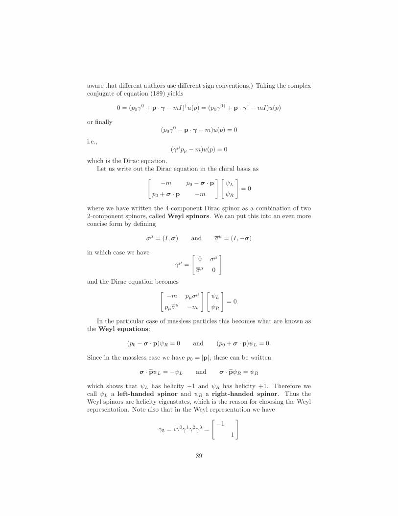
aware that different authors use different sign conventions.) Taking the complexconjugate of equation (189) yields
0 = (p0γ0 + p · γ −mI)†u(p) = (p0γ
0† + p · γ† −mI)u(p)
or finally(p0γ
0 − p · γ −m)u(p) = 0
i.e.,(γµpµ −m)u(p) = 0
which is the Dirac equation.Let us write out the Dirac equation in the chiral basis as
[−m p0 − σ · p
p0 + σ · p −m
][ψL
ψR
]= 0
where we have written the 4-component Dirac spinor as a combination of two2-component spinors, called Weyl spinors. We can put this into an even moreconcise form by defining
σµ = (I,σ) and σµ = (I,−σ)
in which case we have
γµ =
[0 σµ
σµ 0
]
and the Dirac equation becomes
[−m pµσ
µ
pµσµ −m
] [ψL
ψR
]= 0.
In the particular case of massless particles this becomes what are known asthe Weyl equations:
(p0 − σ · p)ψR = 0 and (p0 + σ · p)ψL = 0.
Since in the massless case we have p0 = |p|, these can be written
σ · pψL = −ψL and σ · pψR = ψR
which shows that ψL has helicity −1 and ψR has helicity +1. Therefore wecall ψL a left-handed spinor and ψR a right-handed spinor. Thus theWeyl spinors are helicity eigenstates, which is the reason for choosing the Weylrepresentation. Note also that in the Weyl representation we have
γ5 = iγ0γ1γ2γ3 =
[−1
1
]
89
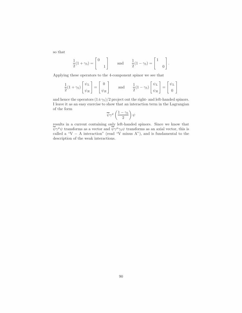
so that
1
2(1 + γ5) =
[0
1
]and
1
2(1− γ5) =
[1
0
].
Applying these operators to the 4-component spinor we see that
1
2(1 + γ5)
[ψL
ψR
]=
[0
ψR
]and
1
2(1− γ5)
[ψL
ψR
]=
[ψL
0
]
and hence the operators (1±γ5)/2 project out the right- and left-handed spinors.I leave it as an easy exercise to show that an interaction term in the Lagrangianof the form
ψγµ
(1− γ5
2
)ψ
results in a current containing only left-handed spinors. Since we know thatψγµψ transforms as a vector and ψγµγ5ψ transforms as an axial vector, this iscalled a “V − A interaction” (read “V minus A”), and is fundamental to thedescription of the weak interactions.
90