The Design of Structured Finance Vehicles · Abstract The Design of Structured Finance Vehicles We model the design of a structured nance deal, speci cally, its capital structure,

The Design of Structured Finance Vehicles

Sanjiv Ranjan DasLeavey School of BusinessSanta Clara University 1

Seoyoung KimLeavey School of BusinessSanta Clara University

December 15, 2014

1We thank Shashwat Alok, Amit Bubna, Donald Davis, Robert Hendershott, YoungdohKim, Bruce Lehman, and Hersh Shefrin for their comments, and seminar participants atCalPERS / the CFA Society, Emory University, the Federal Deposit Insurance Corporation(FDIC), Georgia State University, the Indian School of Business, the Journal of InvestmentManagement (JOIM), the Korea Institute of Finance (KIF), Santa Clara University, andYonsei University. We also thank the Global Association of Risk Professionals (GARP) forfunding support. The authors may be reached at: [email protected], [email protected]; SantaClara University, Department of Finance, Leavey School of Business, Santa Clara, CA95053.

Abstract

The Design of Structured Finance Vehicles

We model the design of a structured finance deal, specifically, its capital structure,

leverage risk controls, asset quality, and the rollover frequency of senior debt. Instead

of providing safety, stringent risk management controls often accelerate failure, and

optimal risk management choices depend critically on the rollover horizon of the se-

nior notes. The expected losses on senior notes become increasingly sensitive to pool

risk (i.e., spread volatility) when risk controls become more stringent, particularly

under shorter rollover horizons. Post the financial crisis, we intend to inform the

creation of safer SPVs in structured finance, and we propose avenues of mitigating

senior note risk through contingent capital.

Keywords: SPVs; SIVs; special purpose vehicle; structured investment vehicle;

structured finance risk controls; structured finance credit ratings; contingent capi-

tal.

1 Introduction 1

1 Introduction

Structured finance deals emerged as an increasingly important means of risk sharing

and obtaining access to capital prior to the financial crisis of 2008. Market segmen-

tation and an ever-increasing demand for safe debt resulted in a marked shift in the

suppliers of safe debt from the commercial banking system to the shadow banking

system, which provided an increasing share of “safe” assets via special purpose vehi-

cles (SPVs), overtaking many traditional sources of safe debt (Gorton, Lewellen, and

Metrick (2012)). At their peak in 2007, Pozsar, Adrian, Ashcraft, and Boesky (2012)

estimate that shadow banking liabilities had grown to nearly $22 trillion.

Given their scope and magnitude, it is crucial to understand this new and highly

complex asset class. For example, before the financial crisis, twenty-nine structured

investment vehicles, none of which remain today, held an estimated $400 billion in

assets.1 Despite their AAA rating, senior notes issued by these SIVs experienced an

average 50% loss, and subordinated notes experienced near total loss.2

From these widespread failures, a natural question arises as to whether the de-

sign of SPVs was adequate to ensure promised repayment to senior note holders

with AAA-level certainty. Did the demise of SPVs in the crisis occur despite careful

security design and risk management practices, or because of it? A parsimonious

theoretical model of structured finance vehicles developed here shows that the locus

of viable SPVs was exceedingly small, and these vehicles were destined to fail with

high probability. Our model also suggests a modified, more resilient SPV structure.

A structured finance deal is engineered to tranche investments in an asset pool

into prioritized cash-flow claims. The resulting liability structure comprises two broad

sources of capital for SPVs: the so-called equity portion, which comprises bonds/notes

1http://www.telegraph.co.uk/finance/newsbysector/banksandfinance/5769361/400bn-SIV-market-sold-off-in-two-years.html

2http://www.risk.net/risk-magazine/news/1517514/almost-siv-assets-sold-fitch

1 Introduction 2

commonly denoted as “capital” notes, and the de facto debt portion of the capital

structure, known as “senior” notes, which are supported by the subordinated capital

notes. The senior notes form the primary source of financing, often accounting for

more than 90% of the liabilities. Structured finance deals are designed with the intent

to secure a AAA rating for the senior notes, which pay slightly above the risk free

rate of interest.

The asset pool of the SPV may comprise a wide range of fixed income and credit

assets, such as corporate bonds, residential mortgage-backed securities (RMBS), com-

mercial mortgage-backed securities (CMBS), as well as other asset-backed securities

(ABS) collateralized by credit card loans, auto loans, home-equity loans, etc. The

quality of assets can range from those rated AAA to below investment grade, and

diversification of the pool along various dimensions is intended to reduce the risks

inherent in these assets.

Designing a deal that is safe for senior note holders is inherently difficult. Studies

have explored the securitization and design of special purpose vehicles in structured

finance, and the attendant benefits to investors and issuers. DeMarzo and Duffie

(1999) examine the role of information and liquidity costs inherent in selling tranches

of a structured finance deal, highlighting the lemons problem in the issuance of asset

backed securities. DeMarzo (2005) demonstrates liquidity efficiencies to creating low

risk senior notes from the pooling and tranching of asset backed securities.

This paper explores very different aspects of structured finance design than has

been considered in the literature so far, and is aimed at determining the optimal

design of a SPV, i.e., the capital structure, risk controls, and rollover horizon of debt

tranches. Many results are counterintuitive, suggesting that a naive approach to SIV

design might exacerbate risk rather than mitigate it. Hence, improperly designed risk

controls for the tranching and pooling of securities can offset the risk diversification

benefits pointed out in DeMarzo (2005).

1 Introduction 3

We summarize our main results. First, we examine the effect of risk controls on

the quality of tranches issued by the SPV, and show that tightening risk controls

may in fact increase risk. We show that tranche ratings and risks are extremely

sensitive to the primary form of risk control— the leverage constraint3 mandated

by the SPV—which if violated, leads to “defeasance”, i.e., early termination of the

vehicle and a liquidation of the SPV’s assets. Paradoxically, tighter risk controls can

increase the ex-ante expected losses of the senior notes because the probability of

defeasance increases sharply when leverage controls are tightened, making the senior

notes more likely to lose value. This effect is more pronounced under greater fire-sale

discounts.

Second, the rollover horizon of the senior notes is a polarizing factor in determin-

ing the most effective level of leverage risk controls, with the optimal leverage control

threshold increasing (i.e., becoming more likely to trigger defeasance) in the rollover

horizon. Overall, tight risk controls are beneficial in the case of long rollover horizons,

but detrimental for short horizons.

Third, ratings volatility increases with risk controls. There are interesting inter-

actions between expected losses (ratings) to the senior note holders and the riskiness

of the asset pool (i.e., spread volatility), the size of the senior tranche, and the level

of the leverage risk control threshold. Under shorter rollover horizons, the expected

losses on senior notes become increasingly sensitive to pool risk as leverage controls

become more stringent. Hence, there is a trade-off between reducing credit risk and

reducing expected loss exposure to pool risk. That is, if senior-note rollover horizons

are shortened and leverage controls are tightened to reduce credit risk, the expected

losses on the senior tranche become more sensitive to the spread volatility of the

underlying asset pool.

3The leverage constraint usually stipulates a minimum allowable ratio of pool assets to seniornotes, i.e., akin to the inverse of a loan-to-value (LTV) ratio. Hence, this leverage trigger is of valuegreater than 1.

1 Introduction 4

Fourth, optimal SPV design is highly sensitive to the expected fire-sale discount

upon defeasance, particularly under longer rollover horizons. For instance, under

standard spread volatility assumptions and an expected fire-sale discount of 10%, an

SPV can issue a senior tranche size of 89.3%, achieving expected losses no greater

than 0.01% if they set the minimum leverage threshold constraint (ratio of assets to

senior notes) to 1.115. However, if the fire-sale discount were slightly greater at 15%,

this senior tranche size / leverage-constraint combination corresponds to an expected

loss to senior notes of 5.2%, which is far greater than the 0.01% cutoff required to

maintain high-quality ratings.4 In fact, under an expected fire-sale discount of 15%,

the maximal attainable high-quality senior tranche size is 85%, with the leverage

threshold constraint set to 1.0. Thus, we see that the chosen SPV design is very

different based on small differences in the expected fire-sale discount upon defeasance.

This consideration is particularly important given the highly uncertain nature

of fire-sale discounts in times of distress, whereby one SPV’s defeasance may easily

trigger that of another SPV, pushing up fire-sale discounts even higher. For instance,

Cheyne Finance recovered 44% of par value in initial liquidation rounds;5 Sigma

Finance recovered 15%.6 Thus, stress tests of SPV design must not only account

for swings in spread volatility (i.e., extreme pool risk) but must also account for the

potentially vast swings in fire-sale discounts under defeasance.

Fifth, contingent capital in SPVs is pareto improving to all classes of debt. When

the defeasance trigger is first hit, capital note holders are required to infuse capital,

paying down a portion of the senior notes and allowing the SPV to continue rather

4We define this cutoff based on the Rating Methodology guide published by Moody’s InvestorsService. See “Probability of Default Ratings and Loss Given Default Assessments for Non-FinancialSpeculative-Grade Corporate Obligors in the United States and Canada,” Global Credit Research,August 2006, page 10, Exhibit 2.

5http://www.risk.net/risk-magazine/news/1504163/cheyne-assets-disappoint-in-rescue-auction.Cheyne was one of the largest SIVs created in 2005 before the onset of the financial crisis. It wasthe first to include subprime assets in its pool.

6http://www.telegraph.co.uk/finance/newsbysector/banksandfinance/5769361/400bn-SIV-market-sold-off-in-two-years.html

1 Introduction 5

than defease. This substantively decreases expected loss rates to both senior and

capital note holders.7

Numerical analysis shows that, for many standard SPV parameters, these vehicles

were designed to fail, and require careful restructuring in order to provide safe returns

to senior note holders. Our findings provide normative prescriptions for the risk

management of structured deals, whereby the risk controls, capitalization, and rollover

horizon interact in a delicate balance to achieve a viable SPV.

Our paper also relates to the recent literature on the risks of securitization. Coval,

Jurek, and Stafford (2009a) discuss the features of securitized pools, where senior

tranches are akin to economic catastrophe bonds, failing under extreme situations,

but offering lower compensation than investors should require. We provide evidence,

in fact, that pervasive risk control design flaws make such bonds more prone to

economic catastrophe, demonstrating why their paper finds these bonds are poor

investments. In related work, Coval, Jurek, and Stafford (2009b) argue that small

errors in parameter estimates of the collateral pool result in a large variation in the

riskiness of the senior tranches. Complementing this asset-side result, we find that

the liability side matters too: irrespective of the risk parameters of the collateral

pool, small changes to risk control level (i.e., the leverage ratio threshold) can cause

large changes to the riskiness and value of the senior tranches, and thus, to the rating

achieved by these notes.

Whereas these papers suggest that systematic extreme risk was not reflected in

senior tranche pricing, they also point out that fire sales matter in increasing corre-

7For instance, consider an SPV issuing two-year notes, with a leverage threshold of 1.04, un-derlying asset spread volatility of 1.05%, and expected fire-sale discount of 10%. In the absenceof pre-committed capital infusions, a 92% senior tranche size has an expected loss rate of 2.87%,indicating that a far smaller senior tranche size is required to secure a AAA rating on senior notes.However, with the use of contingent capital, the expected loss to senior note holders decreases to0.01%, allowing the larger senior tranche size while maintaining a AAA rating. Moreover, the ex-pected loss to capital note holders decreases from 63.27% to 48.13%, thereby benefiting all partiesinvolved.

2 Model 6

lations of distressed assets (see Coval and Stafford, 2007; Shleifer and Vishny, 2010;

Diamond and Rajan, 2011). Similarly, Cont and Wagalath (2012) model the impact

of fire sales in multiple funds on the volatility and correlation of asset returns in a

setting with multiple assets. We show that this is a major factor in the assessment of

risk controls and has a first-order effect in generating wide swings in expected losses,

resulting in lower ratings. In relation to these papers, Hanson and Sunderam (2013)

argue that pooling and tranching creates “safe” senior tranches owned by the major-

ity of investors, leading to a dearth of informed investors in good times and resulting

in insufficient risk controls, which are shown to be weak when bad times arrive. Our

paper argues that stringent risk controls are not always required, and often exacer-

bate the problems experienced from a drop in pool asset values, highlighting a new

form of “neglected” risk (see Gennaioli, Shleifer, and Vishny, 2010).

The rest of the paper proceeds as follows. Section 2 presents the model set up, and

Section 3 shows how the probability of defeasance and expected loss varies with risk

controls, and examines how the size of the senior tranche and its roll-over frequency

impacts risk and ratings. Section 4 examines how the feasible region for high quality

senior note ratings is impacted by the issuing SPV’s design. Section 5 discusses

mitigating risk for senior notes using contingent capital. Section 6 concludes.

2 Model

2.1 Basic Set Up

We develop a parsimonious model of structured finance and SPV design. The aggre-

gate value of the asset pool at time t is denoted as A(t), and the liabilities are denoted

as B(t) for the senior notes, and C(t) for the capital notes and, A(t) = B(t) + C(t).

The face values of the capital and senior notes are denoted DC and DB, respectively.

At inception (i.e., at time t = 0), B(0) = DB and C(0) = DC = A(0)−B(0).

2 Model 7

Investors in senior notes seek safe assets with assured returns, and hence, SPVs are

designed with the intent to attain a AAA credit rating for the senior notes, reflecting

a 0.01% expected loss from default, i.e., the probability of default times the loss on

default is expected to be less than 1/100th of one percent.8 The expected loss is

critically dependent on the following factors:

1. The credit quality of the asset pool (i.e., its mean spread α and spread volatility

σ),

2. The size of the senior tranche (DB) and subordinated equity tranche (DC),

3. The time to rollover/maturity of the senior notes T , and

4. The risk controls outlined by the SPV, i.e., the leverage control level K.

The capital note holders retain the residual after repayment of the senior notes

and management fees borne by the SPV.9 Thus, capital note holders bear first losses

on the SPV’s assets. The SPV makes a spread between the rate of return on the

assets and the rate of interest paid to the senior notes, from which the capital note

holders are compensated. This spread arises because the assets held are of longer

maturity than that of the senior notes that are periodically rolled over. Hence, the

maturity of the senior notes is shorter than that of the capital notes and the weighted

average maturity of the assets of the SPV.

To afford the senior notes additional protection, the SPV covenants typically

include safeguards pertaining to asset quality in addition to requirements regarding

the duration and liquidity of the assets in the collateral pool. In addition to these

asset restrictions, the SPV is monitored on an ongoing basis, primarily through a

8See Cantor, Emery, and Stumpp (2006).9In case the capital note holders are the founders/managers of the SPV, they also collect man-

agement fees.

2 Model 8

leverage test, whereby the ratio of collateral value to senior-note obligations must

meet a pre-specified cutoff.10 Failure to meet these requirements forces the SPV into

“defeasance” or “enforcement” mode, whereby the assets of the SPV must be sold to

wind down operations. The proceeds are used to first pay off the senior note holders,

with the residual used to pay off the equity note holders.

We define an SPV’s leverage at any point in time as

A(t)

DB

≥ K ≥ 1 (1)

where K is the lower bound on the ratio of collateral assets, A(t), to senior notes,

DB, that is permitted by the SPV. For example, an SPV with no equity notes has a

leverage ratio equal to 1, and an SPV with assets worth 100 and senior notes with

a face value of 92, has a leverage ratio of 1.087. Suppose a lower limit of K = 1.04

is placed on the leverage ratio. Then the SPV enters defeasance (enforcement) mode

when A(t) = DB ·K = 92× 1.04 = 95.68, i.e., a 4.32% drop in the value of the assets

held by the SPV, which results in a 54% loss to the capital note investors assuming

a frictionless market with no fire-sale discounts.

In reality, enforcement mode likely occurs when markets are under stress and

other financial institutions (including other SPVs) are also attempting to unwind,

and assets are unlikely to be sold at full market value but rather at fire sale prices,

at some percentage discount δ. Hence, the anticipated recovery is only a fraction

(1− δ) < 1 of the assets’ value at defeasance, i.e., ((1− δ)DBK). Since K ≥ 1, with

diffusion processes for the assets A(t), unless defeasance occurs, the senior notes incur

no losses. If defeasance occurs, then the losses incurred by senior notes amount to

max(0, DB− (1−δ)DBK) = DB max(0, 1− (1−δ)K). Using the illustrative numbers

10Other tests are imposed, such as liquidity and pool composition, but these are less likely to triggerdefeasance than the leverage test, which is essentially a trigger corresponding to a prespecified fallin assets. Thus, the SPV risk model trigger is akin to a barrier in the Black and Cox (1976) class ofstructural default models.

2 Model 9

above, the senior notes will incur losses if (1− (1− δ)K) > 0, i.e., the recovery rate

(1 − δ) is less than 1/K = 1/1.04 = 96.15%, or equivalently, if the fire-sale discount

δ ≥ 3.85%.

In the ensuing analyses, we make the following parameter choices, which are rea-

sonable average values based on usual market statistics about structured finance deals

and the SPVs designed to operationalize them. We choose two sizes of the senior notes

tranche, both common usage, i.e., DB = {0.88, 0.92}, expressed as fractions of the

total asset pool of the SPV. Each of these levels corresponds to equity note levels of

0.12 and 0.08, respectively. We vary the threshold leverage constraint K from 1.0 to

A(0)/DB. The expected fire sale discount upon default, δ, is set to 10% and 15%,

meaning that the recovery rate on asset sales upon defeasance is (1−δ) = {0.90, 0.85},

respectively, for these two levels. The risk free rate is set to be r = 0.02. The senior

notes are rolled over at two horizons, 1 year and 4 years.

The value of the asset pool depends on the current spread at which it is trading

and we denote this as s(t). Asset spread volatility σ is taken to be 65 basis points and

varied up to 105 bps, and in some cases all the way up to 500 bps. For asset-backed

securities, normal spread volatility is in the range of 11–57 bps,11 and the values used

reflect stressed values of standard deviations, commonly used by rating agencies in

their evaluation of SPV structures.

2.2 The State Price of Defeasance

The state price of defeasance is the discounted probability that the SPV will be in

defeasance before the rollover date for senior debt. We define f [τ ] as the first passage

probability density of the defeasance barrier being hit at time τ (i.e., when the assets

drop to defeasance level). The state price of a specific defeasance stopping time τ is

11See Moody’s Special Comment titled “The Relationship between Par Coupon Spreads and CreditRatings in US Structured Finance,” December 2005, by Jian Hu and Richard Cantor.

2 Model 10

e−rτf [τ ]. For a part of the expected loss calculation, we need to compute the integral∫ T0 e−rτf [τ ] dτ , i.e., the state price of defeasance, which is equal to the present value

of a cash-or-nothing binary barrier option that pays $1 the moment the underlying

A(t) touches the barrier DB ·K.

Computing expected loss on the senior notes is simplified if we have the state

price of defeasance, which depends on stochastic changes in the value of the asset

pool, which in turn, depend on the stochastic process for s(t) (the yield increment

on the assets), which we characterize shortly. The price of the asset pool A(t) comes

from discounting assets at the risk free rate plus asset spread, i.e., the current yield

on the assets. The variable s(t) ≥ 0 is a spread widening factor that drives the

asset pool value down from its initial value of A(0) to barrier DB ·K; i.e., we define

A(t) = A(0)e1−s(t). Hence, we normalize s(0) = 1 and then define the barrier level of

s̄ > s(0), such that

A(0)e(1−s̄) = DB ·K (2)

Inverting this equation we have the level of s(t) at which defeasance is triggered as

follows:

s̄ = 1− ln

[DB ·KA(0)

](3)

Assuming a stochastic process for s(t) enables the calculation of the probability of

defeasance in closed form using barrier option mathematics. We assume that this

asset spread widening factor follows a geometric Brownian motion, i.e.,

ds(t) = α s(t) dt+ σ s(t) dW (t), s(0) = 1 (4)

Factor s(t) drives the asset process A(t), where the drift is α, the volatility parameter

is σ, and dW is a Wiener increment. The larger the drift α, and volatility σ, the

greater the probability of defeasance. So, when A(t) makes a first-passage transition

to DB ·K, then s(t) transitions to s̄ (as per equation (3)), with first passage probability

2 Model 11

f [τ ] as defined earlier. Under this process the formula for the discounted first-passage

density for s(0) = 1 reaching s̄, i.e., the probability of defeasance, is as follows:12

∫ T

0e−rτ f [τ ]dτ = s̄ µ+λN(−z) + s̄ µ−λN(−z + 2λσ

√T ) (5)

where

z =ln(s̄)

σ√T

+ λσ√T ; µ =

α− σ2/2

σ2; λ =

√µ2 +

2α

σ2

We note that f [τ ] may be written in more detailed form as follows:

f [τ ] ≡ f [s(τ) = s̄|s(0), s(t) < s̄, 0 ≤ t < τ ]

≡ f [A(τ) = DBK|A(0), A(t) > DBK, 0 ≤ t < τ ] (6)

and the latter expression will be used for further analysis in the paper using the first

passage time density function f [τ ]. We turn to the rating process next.

2.3 Expected Losses and Ratings

Rating agencies run simulated models of the SPV’s assets to determine the expected

losses on the senior notes. Expected losses map into ratings for these notes and hence,

it is important to assess the interaction of risk controls K (the leverage trigger), size

of the senior tranche DB, and spread volatility of assets in the pool (σ) in determining

these expected losses.

The general expression for the present value of expected losses on the senior notes

on defeasance is as follows:

ELB = DB max(0, 1− (1− δ)K) (7)

·∫ T

0e−rτf [A(τ) = DB ·K|A(0), A(t) > DB ·K, 0 ≤ t < τ ] dτ

12See Haug (2006) for details of the cash-or-nothing binary barrier option that forms the basis forthis pricing equation.

2 Model 12

The loss on defeasance is a constant, DB max(0, 1 − (1 − δ)K), which is multiplied

by the cumulative first passage defeasance probability. This equation is separable

in the loss on default and the first passage time probability because the state of

defeasance is a constant barrier, dependent on threshold K, and hence the first-

passage probability is always triggered at the same state. Here, r is the risk free rate,

and f [A(τ) = DB · K|A(0), A(t) > DB · K, ∀t < τ ] is the first-passage probability

of A(t) to barrier DB · K, which we denoted above more parsimoniously as f [τ ].

Equation (5) presents the expression for∫ T0 e−rτf [τ ]dτ , which we can apply directly

in equation (7) to calculate the expected loss, ELB, on the senior notes. As stated

earlier, for senior notes to receive a AAA rating, ELB ≤ 0.01%.

Overall, we see that E(L) > 0 if (1−δ) < 1/K. Note that since K > 1, defeasance

always occurs before default (A(T ) < DB). Thus, at maturity, the assets must be

sufficient to pay the senior notes else defeasance would have occurred earlier. We now

turn to the analysis of various aspects of the SPV structure.

2.4 Stochastic Fire Sale Discount

The model may be extended to accommodate a stochastic fire sale discount δ. This

robustness test shows that the results of the paper remain unaffected even when there

is uncertainty about the the size of the fire sale discount (numerical results presented

in the following section).

We assume a state variable x that drives the fire sale percentage discount δ as

follows.

δ(t) = 1− 1

2

[arctan(x(t))

2

π+ 1

]∈ (0, 1) (8)

where x(t) follows the stochastic process:

dx(t) = κ(θ − x(t)) dt+ η√x(t) dZ, dW · dZ = ρ dt (9)

3 Analysis 13

θ = tan{π

2[2(1− δ0)− 1]

}(10)

Here κ is a mean-reversion rate, η is the volatility of the state variable, and θ is

the level of x when δ(t) = δ0, i.e., the fire sale discount in a model where it is not

stochastic. Here ρ is the correlation between the spread process Wiener shock W (t)

(see equation 4) and the fire sale discount stochastic process δ(t)’s Wiener shock Z(t)

(see equation 9). The fire sale discount is bounded between (0, 1) as may be seen in

the mathematics of equation (8). We note that E[δ(t)] = δ0. As x(t) cycles over time,

so does the fire-sale discount δ(t). For larger portfolios, fire-sale discounts tend to be

larger, and this may be adjusted by setting δ0 appropriately.

Under this framework, we recompute the expected losses to senior notes and com-

pare these values to the ones from equation (7). We do so by simulating the bivariate

density function for {A, δ} at the defeasance barrier. As we will see in the following

section, the difference in results from making the fire sale discount stochastic is not

material. Hence, we impose a pre-determined δ upon defeasance, and employ the

closed form expressions given in the paper.

3 Analysis

Although it is clear that increases in the leverage constraint K must increase the

probability of defeasance, a natural question arises as to how sensitive the probability

of defeasance is to changes in leverage threshold K and how these factors ultimately

affect expected losses to senior note holders. In the event that fire-sale discounts

are high on account of correlated SPV asset pools (see Covitz, Liang, and Suarez,

2013), large changes in the probability of defeasance arising from small changes in the

leverage constraint K, will cause wide swings in expected losses, and consequently in

credit ratings. We call this sensitivity “design” risk, i.e., small perturbations in SPV

3 Analysis 14

risk control design may lead to substantial neglected risks (Gennaioli, Shleifer, and

Vishny (2010)), in this case, high ratings volatility, of which investors are unaware.

Intuitively, we see that leverage controls on an SPV must be implemented with

care to prevent excessive or premature defeasance, which in turn leads to a large quan-

tum of systemic risk if all SPVs implement similar risk controls, possibly triggering

simultaneous defeasance. The resulting selling cascade may lead to even greater fire

sale discounts, which may impose large amounts of risk even on the senior notes. We

now proceed to explore how these factors, in tandem, affect ex-ante expected losses

to senior note holders.

3.1 Risk Management increases Risk

The primary form of risk control in an SPV is the leverage constraint, i.e., the thresh-

old K of leverage at which defeasance is triggered if the assets fall sufficiently in value.

Since the leverage threshold in our model is defined as K = A(t)/DB, we usually ex-

pect an SPV to have a threshold of K > 1, the reason being that triggering defeasance

earlier leaves a greater amount of capital notes to buffer losses that might otherwise

be borne by the senior note holders. However, if we set K too high, then defeasance

may occur too rapidly and increase the likelihood of incurring deadweight costs on

defeasance, which may increase expected losses to the senior tranche. It may even be

optimal to set K below 1, since allowing a drop in the value of the portfolio below the

value of the senior notes may allow the necessary time in which assets can recover,

staving off premature defeasance that would lead to deadweight costs.

In Figures 1 and 2 we implement equation (7), plotting the expected loss on senior

notes as a function of the leverage threshold K for a one-year and four-year horizon,

respectively. We keep the size of the senior tranche fixed at DB = 0.92 (upper panel);

for comparison, we also examine this relation under a senior tranche size of DB = 0.88

(lower panel).

3 Analysis 15

Beginning with Figure 1 (one-year horizon), we observe that the function for

expected loss can also be very sensitive to K, i.e., to the stringency of the leverage

control imposed on the SPV, depending on the size of the senior tranche (DB) and

the expected fire-sale discount upon default (δ). Moreover, the difference in expected

losses under varying fire-sale discounts (δ = {0.10, 0.15}) increases very quickly as

the defeasance trigger, K, increases.

Specifically, we observe that at a lower fire sale discount rate (δ = 0.10), increasing

K does not materially impact the expected losses to the smaller senior tranche size

(DB = 0.88), but expected losses begin to increase dramatically with K at the larger

senior tranche size (DB = 0.92). When the senior notes comprise 92% of the liabilities,

the expected loss at a leverage threshold of K = 1.04 delivers a high-quality rating

(i.e., low expected loss), but as the leverage threshold exceeds K = 1.04, the expected

loss increases rapidly. However, we observe that at a higher fire-sale discount rate

(δ = 0.15), expected losses are very sensitive to K, increasing dramatically for both

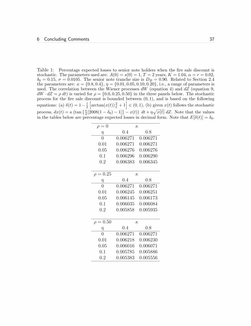
the larger and smaller senior tranche sizes. As a test for robustness the results in

Table 1 show that the expected losses to senior notes remain virtually the same even

when δ is stochastic (see Section 2.4). The level of fire-sale discounts is known to vary

with the size of the liquidated portfolio,13 and this may be modeled in our setting by

varying the mean size of the fire-sale discount through parameter δ0, where we choose

this parameter to be larger for bigger liquidations.

In contrast, from Figure 2 (four-year horizon), we observe that for the larger senior

tranche size of 92%, expected losses increase with K and then begin to decline, though

they remain far too high to justify a AAA rating.For the smaller tranche size of 88%,

we observe that at very high levels of K, expected losses are low enough to justify a

AAA rating, as long as the fire-sale discount is sufficiently low (in this case, 10%).

13Variation in the size of the fire-sale discount with portfolio liquidation size is discussed in Chanand Lakonishok (1995), Chan and Fong (2000), Dufour and Engle (2000), and Bouchad, Farmer,and Lillo (2009).

3 Analysis 16

Thus very high values of K are more helpful under longer horizons, where stringent

leverage controls can make the senior notes safer and assure a higher rating.

We also explore how incorporating jumps may affect our observations. The results,

presented in Figure 3, indicate that even for the smaller tranche size of 88%, expected

losses are generally too high to justify a AAA rating under a four-year horizon when

we include the possibility of a 40% jump with likelihood 0.001 per annum. If we

decrease the jump size to 10%, then we see that for smaller leverage thresholds AAA-

rating is feasible, but under larger thresholds, the expected losses remain far too high.

Intuitively, with fire-sale discounts, the SPV is better off under leverage constraints

with far too low of a probability to be accessed (thereby staving off the fire sale), or

with a beginning Asset-to-DB ratio that is sufficiently high so as to make it improbable

to access a leverage constraint (something that is only possible with a sufficiently small

senior tranche size).

Overall, we see that the rating of the SPV can be extremely sensitive to leverage

risk controls, and this sensitivity hinges critically on the expected fire-sale discount

upon defeasance, highlighting a fundamental flaw in SPV design: i.e., the insufficient

attention paid to the magnitude of fire-sale discounts on defeasance. Indeed many

of the models used by rating agencies in practice did not explicitly account for fire

sale discounts, calling into doubt the ex-ante AAA ratings assigned prior to the 2008

crisis.

Ultimately, in some cases, it is more beneficial to set the defeasance point K

sufficiently high so as to ensure an adequate capital notes buffer for the senior notes.

In other cases, it is more beneficial to set the defeasance point low enough so as to

allow sufficient time for the assets to recover. The designated prescription changes

substantially with the fire sale discount, since setting stringent risk controls, i.e.,

high defeasance triggers, is especially risky during poor economic times when fire-sale

discounts tend to be high. In short, risk controls fail to do their job in precisely those

3 Analysis 17

states of the economy when they are needed the most. As experienced in the 2008

financial crisis, stringent controls trigger were tripped for many SPVs simultaneously,

exacerbating this problem. Thus, it may in fact be better to set very low thresholds

or no leverage constraint at all. In the final section of the paper, we recommend a

solution using contingent capital calls.

3.2 Sensitivity to Pool Risk

With recent notable failures of structured finance deals, much blame has been placed

on the poor quality of assets held by SPVs (e.g., subprime mortgages). The extant

ratings process for SPVs revolves around determining pool risk level σ for rating

agency simulation models. If estimation risk for this parameter is high, then ratings

are likely to be noisy measures of senior note credit quality. Thus, natural questions

arise as to how much expected losses are affected by underlying pool risk, whether

this was indeed a primary source of risk, and what are the factors either mitigating

or exacerbating its importance.

We examine these issues in two ways. First, we contrast the results from Figures

1 and 2 with changing pool risk, i.e., we vary parameter σ in order to understand

how expected losses vary as this parameter changes. Second, we examine whether

this relation is attenuated or exacerbated by changes to the leverage threshold. If

sensitivity to pool risk increases with the tightening of leverage constraints, then risk

controls are especially tenuous just when they are most needed. Finally, we examine

how these sensitivities are affected by varying combinations of senior-tranche size and

rollover horizon.

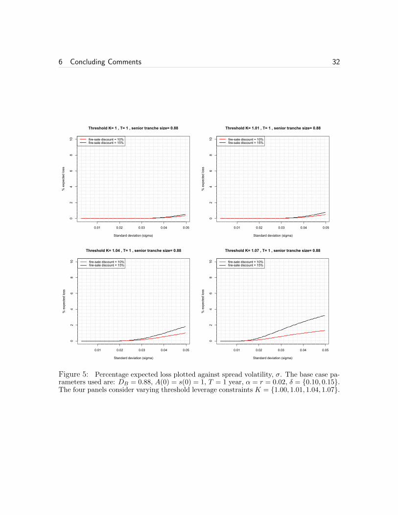
In Figures 4, 5, 6, and 7, we plot percentage expected losses on senior notes

against σ under varying tranche sizes, horizons, and thresholds. For both smaller

and larger senior tranche sizes, we observe that under the shorter one-year rollover

horizons (Figures 4 and 5), the expected losses on senior notes become increasingly

4 Locus of Acceptable Ratings 18

sensitive to pool risk as leverage controls become more stringent. That is, under

greater levels of K, expected losses increase even more with increases in σ. Under

the longer four-year horizon, we observe that expected losses under the larger senior

tranche size (Figure 6) are not increasingly sensitive to pool risk as K is increased,

but overall, expected losses are too high to sustain a AAA rating. Under the smaller

senior tranche size (Figure 7), we observe an initial increase in the sensitivity to pool

risk as K is increased, then the sensitivity to pool risk begins to decline at even

greater values of K (by which point, the expected losses become too high to support

a AAA rating).

Overall, we find that increasing asset pool risk (σ) usually (but not always) makes

it less likely to achieve viable top quality ratings for the senior notes. Therefore asset

quality is material, even if risk management is appropriately tuned. This problem

is exacerbated if risk controls (K) are tightened, complicating the intuition that

adequate risk controls are helpful in managing credit risk in SPVs, because stringent

risk controls make expected losses higher in the presence of fire sale discounts (δ),

in addition to making expected losses more sensitive to asset pool risk. These issues

suggest that efficacious structured finance and SPV design is surprisingly hard to

achieve, and offer insights into the dramatic failure of structured finance deals during

the recent financial crisis.

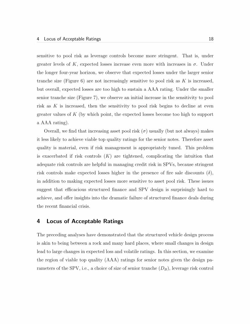
4 Locus of Acceptable Ratings

The preceding analyses have demonstrated that the structured vehicle design process

is akin to being between a rock and many hard places, where small changes in design

lead to large changes in expected loss and volatile ratings. In this section, we examine

the region of viable top quality (AAA) ratings for senior notes given the design pa-

rameters of the SPV, i.e., a choice of size of senior tranche (DB), leverage risk control


(K), and rollover horizon (T ). The SPV design problem, from the viewpoint of the

originator / capital note holders, is to select the leverage constraint K and rollover

horizon T that allows us to maximize the size of the senior tranche DB while keeping

the expected loss sufficiently small (i.e., less than or equal to 0.01%) to deliver a AAA

rating on the senior notes.

maxK,T

DB, s.t.ELBDB

≤ 0.01% (11)

Due to market segmentation, the senior notes tranche must be large to benefit the

originators / capital note holders. We examine this issue by plotting the locus of

pairs of {DB, K} (keeping T fixed) that deliver expected percentage losses no greater

than 0.01% under six sets of spread volatility and fire-sale discount configurations:

σ = {0.0065, 0.0105, 0.0500} × δ = {0.10, 0.15}, keeping the riskless rate fixed at

r = 0.02. All parameters are within economically reasonable ranges, barring the high-

stress case of σ = 0.05.14 Typical structured finance rating procedures undertaken by

rating agencies call for stressing the one standard deviation move in asset spreads by

a factor of 2x to 5x, and 500 basis points is a typically high stress case.

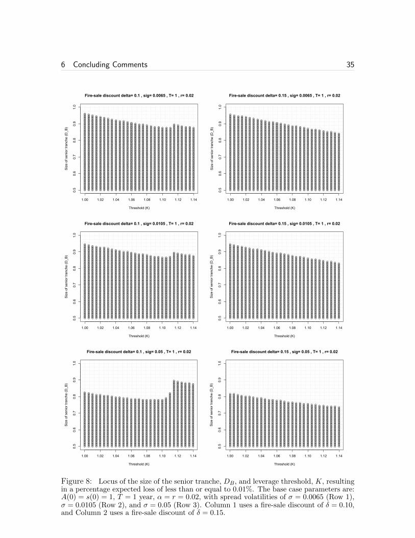
In Figure 8, we present the results based on a rollover horizon of T = 1 year, and

in Figure 9, we present the results based on a rollover horizon of T = 4 years. We

make the following observations:

1. Both Figures 8 and 9 show a decreasing acceptable size of the senior notes

tranche (DB) as we increase the spread volatility (σ) of the asset pool (reading

down the columns in the figure). The range of viable SPV structures also

decreases as we increase the fire-sale discount δ (reading across the rows in the

figure), and this difference becomes starker as we increase the rollover horizon.

14We also explored the case of σ = 0.02 (untabulated) that is qualitatively similar to that ofσ = 0.0105 under both the shorter and longer rollover horizons.


Strikingly, at a longer rollover horizon of T = 4 years, the larger senior tranche

sizes are viable under very strict leverage thresholds (K) when the fire-sale

discount is δ = 10%, but at a greater fire-sale discount of δ = 15%, we observe

that larger senior tranche sizes are not viable even when pushing up the leverage

threshold K. Thus, optimal SPV design is highly sensitive to even small changes

in the fire-sale discount, particularly when the rollover horizon is long.

2. We note that in the financial crisis, the effective fire sale discount was in the

range of δ = 50% to 75%, and our examples are provided for cases of δ =

{10%, 15%}, i.e., highly conservative discounts more in line with one-off SPV

failure, rather than the systemic failures evidenced in the recent past. Even at

these low levels of fire sale discounts, for reasonable levels of risk, the maximal

senior note tranche is DB = 90% approximately, somewhat lower than the levels

seen in practice (for example, the famous Cheyne deal that failed in August

2007, had a senior note tranche size of 92%). Thus, at reasonable stressed levels

of pool risk, it is difficult to justify senior tranche sizes that were observed in

practice.

3. Overall, under the shorter rollover horizon of T = 1 year, optimal SPV design

is not sensitive to the fire-sale discount under more common ranges of spread

volatility (i.e., under σ = {0.0065, 0.0105}), yielding the same decision in the

maximal senior tranche size that can accommodate an expected loss no greater

than 0.01%. However, under the high-stress case of σ = 0.05, optimal SPV

design is highly sensitive to even small changes in the expected fire-sale discount

upon default, whereby the maximum possible senior tranche size is close to 0.90

if the fire-sale discount is δ = 10% but is closer to 0.80 if the fire-sale discount

is δ = 15%. Furthermore, at δ = 10%, the optimal design requires a high level

of K, whereas at δ = 15% the optimal design mandates a very low level of

5 Repairing SPVs 21

K. Hence, for small changes in δ, the optimal risk control changes from one

extreme to the other. This again highlights the vast difficulty in designing an

SPV optimally, especially if uncertainty regarding the fire sale discount δ is very

high.

4. Under a longer rollover horizon of T = 4 years, the optimal SPV design is

sensitive to the expected fire-sale discount even under the more likely ranges

of spread volatility (i.e., under σ = {0.0065, 0.0105}), yielding slight differ-

ences in the maximal senior tranche size that can accommodate an expected

loss no greater than 0.01%. This difference becomes even more dramatic un-

der the high-stress case of σ = 0.05, with a maximal senior tranche size close

to 0.90 if the fire-sale discount is δ = 10%, but a maximal senior tranche size

slightly greater than 0.60 if the fire-sale discount is δ = 15%. Once again the

prescriptions for risk controls for the two fire sale discount values entail polar

opposite outcomes, once again affirming that, irrespective of rollover horizon,

small changes in the expected fire sale discount imply vastly different risk man-

agement protocols.

5 Repairing SPVs

The preceding critique of SPVs suggests that static risk controls with large losses on

defeasance offer no soft landing for senior note holders in times of financial crises,

indicating that senior note holders should be further compensated for the “neglected

risks” they bear, see Gennaioli, Shleifer, and Vishny (2010). These additional benefits

may be dynamic and state-dependent, resulting in a value transfer from capital notes

to senior notes in poor states of the world.

A simple prescription for risk buffering the senior note holders is to build in con-

tingent capital, whereby capital note holders (or the issuer/manager) are required to

5 Repairing SPVs 22

provide additional capital to buy back a sufficient quantity of senior notes at par,

thus returning the leverage ratio to a safe level. This dynamic risk management ap-

proach is similar to a margin call, whereby the extra infusion/buyback is analogous

to the variation margin. Ex-ante, this built-in capital call discourages the creation

of an SPV that the issuer/manager knows to be too risky, and promotes an equi-

librium where only viable SPVs are created.15 Payment of contingent capital could

be ensured by credit or liquidity guarantees, much in the way that conduit spon-

sors of fully supported ABCP (asset backed commercial paper) guarantee payment

(Acharya, Schnabl, and Suarez (2013)); though, the contingent capital we prescribe

below would be far less than full support.

We now examine the net benefits of capital calls. Our chosen method requires

that when the defeasance trigger is hit at stopping time τ , i.e., when the assets fall to

a level such that A(t)/DB = K, then we have a capital infusion by the capital note

holders (or SPV orignator/underwriter) that pays down DB to some level D′B < DB

such that A(t)/D′B > K. This remedy recapitalizes the SPV, replacing senior notes

with capital notes, with no change in the assets of the SPV.

Hence, the senior notes are reset with fresh horizon (T−τ) and for a lower principal

D′B(τ), when the leverage constraint is violated, i.e., A(τ) = DB · K < 1. This

remedy effectively postpones the liquidation of the SPV, and postpones or possibly

eliminates the deadweight fire sale losses on defeasance, allowing time for the SPV’s

assets to recover. The capital note holders also stand to benefit when deadweight

costs are delayed or possibly even eliminated if the prices of the underlying assets

rise, but they bear the costs of this waiting period since they are the ones providing

the additional capital. Thus, although senior note holders are definitively better off

15Basel III envisages requiring contingent capital in addition to Tier 1 capital from banks. Whilethis is not yet under consideration in the US, in September 2011, the Independent Commission onBanking recommended that UK banks be required to hold an additional 7-10% of contingent capital,also known as bail-in capital, where debt would automatically convert to equity on breaching a triggerlevel of leverage.

5 Repairing SPVs 23

when the SPV’s covenants require contingent capital infusions, the question remains

as to whether the capital note holders are better off as well.

We now proceed to evaluate expected losses to the capital note holders, assuming

first that no restructuring is permitted. The expected loss comprises two components:

(a) the expected loss on defeasance prior to rollover date, and (b) the expected loss

when there is no defeasance until the rollover date. The present value of total expected

loss can be expressed as follows:

ELC ≡ L[A0, DB, DC , K, δ, r, T ] (12)

= [DC −min(0, DBK(1− δ)−DB)]∫ T

0e−rτ × f [A(τ) = DBK] dτ

+e−rT∫ A0

DBK[A0 − A(T )] · Pr[A(T )|A(t) > DBK, ∀t] dA(T )

= [DC −min(0, DBK(1− δ)−DB)]∫ T

0e−rτ × f [A(τ) = DBK] dτ

+e−rTA0

∫ 1

s̄[1− e1−s(T )] · Pr[s(T )|s(t) < s̄,∀t] ds(T )

where, as before, f [A(τ) = DBK] is a more concise expression for the first-passage

probability of assets to defeasance boundary DBK. The first line of this equation

pertains to expected loss on defeasance prior to T , and the second line calculates ex-

pected loss at T . Pr[A(T )|A(t) > DBK, ∀t] is the conditional probability of stochastic

terminal value A(T ), given no defeasance prior to maturity. The last line comprises

a change of variable from A(t) to s(t).

We now proceed to evaluate expected losses to the capital note holders, assuming

a pre-commitment to infuse capital, rather than defease, when the leverage threshold

is hit. We denote this new level of expected losses as EL′C . The original first-passage

probability to defeasance was based on a senior note level of DB, but is now based

on the level D′B(τ) < DB instead. Hence, the revised expected present value of losses

5 Repairing SPVs 24

to capital note holders is given by the nested equation:

EL′C = (DB −D′B(τ))∫ T

0e−rτ · f [A(τ) = DBK] dτ (13)

+∫ T

0L[A(0), D′B(τ), DC , K, δ, r, T − τ ] · e−rτ · f [A(τ) = DBK] dτ

+e−rT∫ A(0)

DBK[A(0)− A(T )] · Pr[A(T )|A(t) > DBK, ∀t] dA(T )

where the function L[·] comes from equation (12). The first line in the expression

above accounts for the expected infusion by capital note holders in the amount DB−

D′B, the second line accounts for the expected loss should defeasance occur (after

infusion), and the third line accounts for the expected loss to capital note holders

when there is no defeasance.

We employ a fast simulation approach for computing ELC and EL′C . Overall, the

net gain to capital note holders from restructuring the SPV is as follows:

∆ELC = ELC − EL′C (14)

The sign of this term is indeterminate and depends on the parameters of the SPV;

i.e., the leverage threshold K, the initial size of the senior tranche DB, the expected

fire-sale discount δ, the spread volatility σ, the risk-free rate r, and the investment

horizon T , as well as the pre-committed infusion amount upon triggering the leverage

constraint. If positive, then the scheme is Pareto optimal; otherwise, it represents

wealth transfer from capital note holders to senior note holders. As fire sale discounts

δ increase, we expect that the scheme is more likely to be Pareto optimal.16

In Table 2, we present examples of contingent-capital commitments that transform

an unviable SPV, of unit asset value, to one with AAA-rated senior notes. Specifically,

16This computation ignores the possible increase in capital requirements for the SPV sponsorwhen required to keep contingent capital. Hence, it is an upper bound on the savings to capital noteholders from creating a SPV with remediation by contingent capital.

5 Repairing SPVs 25

under an expected fire-sale discount of δ = 10%, the given SPV parameters support

a senior tranche size of DB = 0.88, which corresponds to an expected percentage

loss to senior note holders of 0.01%. Under a senior tranche size of DB = 0.90, this

expected loss jumps up to 0.39%. However, with a pre-committed infusion of 0.02

upon hitting the leverage threshold, the expected loss to senior note holders drops

to 0.01%, and the expected loss to capital note holders also decreases, from 40.13%

to 38.32%. Moreover, the probability of defeasance decreases from 6.18% to 0.13%.

Under a senior tranche size of DB = 0.92, we see an expected loss of 2.87% in the

absence of contingent capital. Thus using contingent capital results in both senior

notes and capital notes becoming better off.

In addition to these recapitalizing approaches, we can attempt other remedies as

well. For example, senior notes can be paid a rate of interest that is indexed to their

rating or to that of the pool. As the rating falls, higher rates can be paid based on

a predetermined menu, whereby the capital to make such payments come from the

management fees first, and then from cash flows to capital note holders. Ex-post, this

approach compensates the senior notes for bearing additional risk, though payment of

the higher rate is contingent on the SPV’s survival. More importantly, this approach

discourages the SPV’s issuers ex-ante from constructing an SPV they know to be

fragile.

Alternatively, we can restore the value of the asset pool by requiring the SPV

issuer/manager to purchase the lower rated assets that have dropped in value and

to replace them with top quality assets, bringing the leverage ratio A(t)/DB back to

being greater than K. In effect, the capital note holders write credit protection (i.e.,

a spread option) on the pool’s lower rated assets, that is triggered when the value of

the asset pool drops below the leverage threshold, but does not lead to liquidation of

the SPV. Once again, this ex-ante prevents knowingly fragile structured finance deal

from being created.

6 Concluding Comments 26

Ultimately, in any of these remedies, “own” risk of the capital note holders is

certainly an issue. However, given that such SPVs are usually issued by deep-pocket

financial firms (or too-big-to-fail banks), own risk is less of a factor.

6 Concluding Comments

We develop a parsimonious model to analyze the design of structured finance deals and

the special purpose vehicles (SPVs) created to operationalize them. Our findings are

as follows: First, tightening risk management controls can dramatically increase ex-

ante expected losses to senior note holders. Second, the presence of fire-sale discounts,

i.e., deadweight costs of defeasance, leads to fragile structures that are not designed

to sustain the levels of risk, or to ensure repayment of principal to senior note holders

commensurate with a top quality credit rating. Third, optimal risk management

choices qualitatively depend on the rollover horizon of the senior notes. Fourth, senior

note ratings are very sensitive to leverage controls. Fifth, expected-loss sensitivity to

pool risk (i.e., spread volatility of the underlying assets) increases dramatically with

increases in leverage risk controls under shorter rollover horizons. The confluence

of these design characteristics suggests that SPVs were not as resilient to economic

shocks as they should have been, and features of the design contributed to the demise

of many SPVs.

Overall, the fact that ratings and risks are highly sensitive to the fire-sale dis-

count, pool volatility, and risk controls suggests that the senior tranche should be

much smaller, and that more capital notes (i.e. a larger equity tranche) are required

to sustain high-quality ratings on senior notes, as suggested by Admati and Hell-

wig (2013), and by Hanson and Sunderam (2013). We recommend using contingent

capital remedies that make the senior notes safer, while also improving the quality

of the capital notes. Whereas contingent capital offers remediation ex-post to SPV


vulnerabilities, it also likely prevents unviable SPVs from being created ex-ante, since

some of the ex-post costs are borne by the creators of the SPV through their holdings

of capital notes.

The financial crisis of 2008 was largely marked by the failure of structured finance

in general, and special purpose vehicles in particular. This analysis of the pathology

of the crisis and recommendations for remediation provides guidance for the future

evolution of the shadow banking sector.


1.00 1.02 1.04 1.06 1.08 1.10 1.12 1.14

02

46

8

sig= 0.0065 , T= 1 , senior tranche size= 0.92

Threshold (K)

% e

xpec

ted

loss

fire-sale discount = 10%fire-sale discount = 15%

1.00 1.02 1.04 1.06 1.08 1.10 1.12 1.14

02

46

8


Threshold (K)

% e

xpec

ted

loss


Figure 1: Percentage expected loss plotted against the leverage threshold, K. The basecase parameters used are: A(0) = s(0) = 1, T = 1 years, α = r = 0.02, σ = 0.0065,δ = {0.10, 0.15}. The two panels consider varying sizes of the senior tranche, i.e., DB ={0.92, 0.88}.


1.00 1.02 1.04 1.06 1.08 1.10 1.12 1.14

02

46

810

12


Threshold (K)

% e

xpec

ted

loss


1.00 1.02 1.04 1.06 1.08 1.10 1.12 1.14

02

46

810

12


Threshold (K)

% e

xpec

ted

loss


Figure 2: Percentage expected loss plotted against the leverage threshold, K. The basecase parameters used are: A(0) = s(0) = 1, T = 4 years, α = r = 0.02, σ = 0.0105,δ = {0.10, 0.15}. The two panels consider varying sizes of the senior tranche, i.e., DB ={0.92, 0.88}.


0.4 0.6 0.8 1.0

0.00

0.02

0.04

0.06

D_B= 0.88 , sig= 0.0105 , T= 4 ,delta= 0.15 , jump= 0.4

Leverage threshold K

% e

xpec

ted

loss

0.4 0.6 0.8 1.0

0.00

0.02

0.04

0.06



% e

xpec

ted

loss

0.4 0.6 0.8 1.0 1.2

0.000

0.002

0.004

0.006

0.008

0.010

0.012



% e

xpec

ted

loss

0.4 0.6 0.8 1.0 1.2

0.000

0.002

0.004

0.006

0.008

0.010



% e

xpec

ted

loss

Figure 3: Percentage expected loss plotted against the leverage threshold, K, whenincorporating jumps j = {0.10, 0.40}. The base case parameters used are: A(0) = s(0) = 1,senior tranche DB = {0.92, 0.88}, T = 4 years, α = r = 0.02, σ = 0.0105, δ = 0.15. Jumpsoccur at a likelihood of 0.001 per annum. The red horizontal line indicated the 0.01%threshold required to maintain a AAA-rating.


0.01 0.02 0.03 0.04 0.05

02

46

810

Threshold K= 1 , T= 1 , senior tranche size= 0.92

Standard deviation (sigma)

% e

xpec

ted

loss


0.01 0.02 0.03 0.04 0.05

02

46

810

Threshold K= 1.01 , T= 1 , senior tranche size= 0.92


% e

xpec

ted

loss


0.01 0.02 0.03 0.04 0.05

02

46

810



% e

xpec

ted

loss


0.01 0.02 0.03 0.04 0.05

02

46

810



% e

xpec

ted

loss


Figure 4: Percentage expected loss plotted against spread volatility, σ. The base case pa-rameters used are: DB = 0.92, A(0) = s(0) = 1, T = 1 year, α = r = 0.02, δ = {0.10, 0.15}.The four panels consider varying threshold leverage constraints K = {1.00, 1.01, 1.04, 1.07}.


0.01 0.02 0.03 0.04 0.05

02

46

810



% e

xpec

ted

loss


0.01 0.02 0.03 0.04 0.05

02

46

810



% e

xpec

ted

loss


0.01 0.02 0.03 0.04 0.05

02

46

810



% e

xpec

ted

loss


0.01 0.02 0.03 0.04 0.05

02

46

810



% e

xpec

ted

loss


Figure 5: Percentage expected loss plotted against spread volatility, σ. The base case pa-rameters used are: DB = 0.88, A(0) = s(0) = 1, T = 1 year, α = r = 0.02, δ = {0.10, 0.15}.The four panels consider varying threshold leverage constraints K = {1.00, 1.01, 1.04, 1.07}.


0.01 0.02 0.03 0.04 0.05

05

1015



% e

xpec

ted

loss


0.01 0.02 0.03 0.04 0.05

05

1015



% e

xpec

ted

loss


0.01 0.02 0.03 0.04 0.05

05

1015



% e

xpec

ted

loss


0.01 0.02 0.03 0.04 0.05

05

1015



% e

xpec

ted

loss


Figure 6: Percentage expected loss plotted against spread volatility, σ. The base case pa-rameters used are: DB = 0.92, A(0) = s(0) = 1, T = 4 years, α = r = 0.02, δ = {0.10, 0.15}.The four panels consider varying threshold leverage constraints K = {1.00, 1.01, 1.04, 1.07}.


0.01 0.02 0.03 0.04 0.05

05

1015



% e

xpec

ted

loss


0.01 0.02 0.03 0.04 0.05

05

1015



% e

xpec

ted

loss


0.01 0.02 0.03 0.04 0.05

05

1015



% e

xpec

ted

loss


0.01 0.02 0.03 0.04 0.05

05

1015



% e

xpec

ted

loss


Figure 7: Percentage expected loss plotted against spread volatility, σ. The base case pa-rameters used are: DB = 0.88, A(0) = s(0) = 1, T = 4 years, α = r = 0.02, δ = {0.10, 0.15}.The four panels consider varying threshold leverage constraints K = {1.00, 1.01, 1.04, 1.07}.


1.00 1.02 1.04 1.06 1.08 1.10 1.12 1.14

0.5

0.6

0.7

0.8

0.9

1.0

Fire-sale discount delta= 0.1 , sig= 0.0065 , T= 1 , r= 0.02

Threshold (K)

Siz

e of

sen

ior t

ranc

he (D

_B)

1.00 1.02 1.04 1.06 1.08 1.10 1.12 1.14

0.5

0.6

0.7

0.8

0.9

1.0


Threshold (K)S

ize

of s

enio

r tra

nche

(D_B

)

1.00 1.02 1.04 1.06 1.08 1.10 1.12 1.14

0.5

0.6

0.7

0.8

0.9

1.0


Threshold (K)

Siz

e of

sen

ior t

ranc

he (D

_B)

1.00 1.02 1.04 1.06 1.08 1.10 1.12 1.14

0.5

0.6

0.7

0.8

0.9

1.0


Threshold (K)

Siz

e of

sen

ior t

ranc

he (D

_B)

1.00 1.02 1.04 1.06 1.08 1.10 1.12 1.14

0.5

0.6

0.7

0.8

0.9

1.0


Threshold (K)

Siz

e of

sen

ior t

ranc

he (D

_B)

1.00 1.02 1.04 1.06 1.08 1.10 1.12 1.14

0.5

0.6

0.7

0.8

0.9

1.0


Threshold (K)

Siz

e of

sen

ior t

ranc

he (D

_B)

Figure 8: Locus of the size of the senior tranche, DB, and leverage threshold, K, resultingin a percentage expected loss of less than or equal to 0.01%. The base case parameters are:A(0) = s(0) = 1, T = 1 year, α = r = 0.02, with spread volatilities of σ = 0.0065 (Row 1),σ = 0.0105 (Row 2), and σ = 0.05 (Row 3). Column 1 uses a fire-sale discount of δ = 0.10,and Column 2 uses a fire-sale discount of δ = 0.15.


1.00 1.02 1.04 1.06 1.08 1.10 1.12 1.14

0.5

0.6

0.7

0.8

0.9

1.0


Threshold (K)

Siz

e of

sen

ior t

ranc

he (D

_B)

1.00 1.02 1.04 1.06 1.08 1.10 1.12 1.14

0.5

0.6

0.7

0.8

0.9

1.0


Threshold (K)S

ize

of s

enio

r tra

nche

(D_B

)

1.00 1.02 1.04 1.06 1.08 1.10 1.12 1.14

0.5

0.6

0.7

0.8

0.9

1.0


Threshold (K)

Siz

e of

sen

ior t

ranc

he (D

_B)

1.00 1.02 1.04 1.06 1.08 1.10 1.12 1.14

0.5

0.6

0.7

0.8

0.9

1.0


Threshold (K)

Siz

e of

sen

ior t

ranc

he (D

_B)

1.00 1.02 1.04 1.06 1.08 1.10 1.12 1.14

0.5

0.6

0.7

0.8

0.9

1.0


Threshold (K)

Siz

e of

sen

ior t

ranc

he (D

_B)

1.00 1.02 1.04 1.06 1.08 1.10 1.12 1.14

0.5

0.6

0.7

0.8

0.9

1.0


Threshold (K)

Siz

e of

sen

ior t

ranc

he (D

_B)

Figure 9: Locus of the size of the senior tranche, DB, and leverage threshold, K, resultingin a percentage expected loss of less than or equal to 0.01%. The base case parameters are:A(0) = s(0) = 1, T = 4 years, α = r = 0.02, with spread volatilities of σ = 0.0065 (Row 1),σ = 0.0105 (Row 2), and σ = 0.05 (Row 3). Column 1 uses a fire-sale discount of δ = 0.10,and Column 2 uses a fire-sale discount of δ = 0.15.


Table 1: Percentage expected losses to senior note holders when the fire sale discount isstochastic. The parameters used are: A(0) = s(0) = 1, T = 2 years, K = 1.04, α = r = 0.02,δ0 = 0.15, σ = 0.0105. The senior note tranche size is DB = 0.90. Related to Section 2.4the parameters are: κ = {0.8, 0.4}, η = {0.01, 0.05, 0.10, 0.20}, i.e., a range of parameters isused. The correlation between the Wiener processes dW (equation 4) and dZ (equation 9,dW · dZ = ρ dt) is varied for ρ = {0.0, 0.25, 0.50} in the three panels below. The stochasticprocess for the fire sale discount is bounded between (0, 1), and is based on the following

equations: (a) δ(t) = 1− 12

[arctan(x(t)) 2

π + 1]∈ (0, 1), (b) given x(t) follows the stochastic

process, dx(t) = κ(tan

{π2 [2008(1− δ0)− 1]

}− x(t)

)dt+ η

√x(t) dZ. Note that the values

in the tables below are percentage expected losses in decimal form. Note that E[δ(t)] = δ0.

ρ = 0 κη 0.4 0.80 0.006271 0.006271

0.01 0.006271 0.0062710.05 0.006276 0.0062760.1 0.006296 0.0062900.2 0.006383 0.006345

ρ = 0.25 κη 0.4 0.80 0.006271 0.006271

0.01 0.006245 0.0062510.05 0.006145 0.0061730.1 0.006035 0.0060840.2 0.005858 0.005935

ρ = 0.50 κη 0.4 0.80 0.006271 0.006271

0.01 0.006218 0.0062300.05 0.006016 0.0060710.1 0.005785 0.0058860.2 0.005383 0.005556


Table 2: Percentage expected losses to senior versus capital note holders, denoted ELBand ELC , respectively. This table compares the expected losses under a structure that doesnot allow capital infusions to the expected losses under a structure that does. The basecase parameters used are: A(0) = s(0) = 1, T = 2 years, K = 1.04, α = r = 0.02, δ = 0.10,σ = 0.0105. DB denotes the initial senior tranche size, DC denotes the capital-note tranchesize, and Pr(def) denotes the probability (%) of defeasance. infuse denotes the amountto be infused, if any, upon triggering the leverage threshold K; i.e., capital-note holderspurchase a fixed amount of debt back from senior-note holders, thereby allowing the SPVto continue rather than defease.

DB DC infuse ELB(%) ELC(%) Pr(def)

0.88 0.12 — 0.01 31.93 0.13

0.90 0.10 — 0.39 40.13 6.180.90 0.10 0.02 0.01 38.32 0.13

0.92 0.08 — 2.87 63.27 45.610.92 0.08 0.04 0.01 48.13 0.13

References 39

References

Acharya, Viral., Philipp Schnabl, and Gustavo Suarez (2013). “Securitization without

Risk Transfer,” Journal of Financial Economics, 107, 515-536.

Admati, Anat., and Martin Hellwig (2013). “The Banker’s New Clothes: What’s

Wrong with Banking and What to do About It,” Princeton University Press, New

Jersey.

Black, Fischer., and John Cox, (1976). “Valuing Corporate Securities: Some Effects

of Bond Indenture Provisions,” Journal of Finance 31(2), 351–367.

Bouchaud, Jean-Philippe, J. Doyne Farmer, and Fabrizio Lillo (2009). “How markets

slowly digest changes in supply and demand,” in Handbook of Financial Markets:

Dynamics and Evolution, Handbooks in Finance, North-Holland, chapter 2, 57–160.

Cantor, Richard., Kenneth Emery, Pamela Stumpp (2006). “Probability of Default

Ratings and Loss Given Default Assessments for Non-Financial Speculative-Grade

Corporate Obligors in the United States and Canada,” Moody’s Investors Service

- Global Credit Research, New York.

Chan, Louis K. C., and Josef Lakonishok (1995). “The behavior of stock prices around

institutional trades,” The Journal of Finance 50(4), 1147–1174.

Chan, Kalok, and Wai-Ming Fong (2000). “Trade size, order imbalance, and the

volatility volume relation,” Journal of Financial Economics 57(2), 247–273.

Cont, Rama., and Lakshithe Wagalath (2012). “Fire Sale Forensics: Measur-

ing Endogenous Risk,” Available at SSRN: http://ssrn.com/abstract=2051013 or

http://dx.doi.org/10.2139/ssrn.2051013.

References 40

Cordell, Larry., Yilin Huang, and Meredith Williams (2011). “Collateral Damage:

Sizing and Assessing the Subprime CDO Crisis,” Federal Reserve Bank of Philadel-

phia, Working paper 11-30.

Coval, Joshua., and Erik Stafford (2007). “Asset Fire Sales (and Purchases) in Equity

Markets,” Journal of Financial Economics 86, 479–512.

Coval, J., Jurek,J., Stafford,E., (2009a). “Economic Catastrophe Bonds, American

Economic Review 99, 628–666.

Coval, J., Jurek,J., Stafford,E., (2009b). “The Economics of Structured Finance,”

Journal of Economic Perspectives 23, 3–25.

Covitz, D., Liang, N., and Suarez, G.A. (2013). “The Evolution of a Financial Crisis:

Collapse of the Asset-Backed Commercial Paper Market,” Journal of Finance 68,

815-848.

DeMarzo, Peter., and Darrell Duffie (1999). “A Liquidity-Based Model of Security

Design,” Econometrica 67(1), 65-99.

DeMarzo, Peter. (2005). “The Pooling and Tranching of Securities,” Review of Fi-

nancial Studies 18(1), 1–35.

Diamond, Douglas., and Raghuram Rajan (2011). “Fear of Fire Sales, Illiquidity

Seeking, and the Credit Freeze,” Quarterly Journal of Economics 126, 557–591.

Dufour, Alfonso, and Robert F. Engle (2000). “Time and the price impact of a trade,”

The Journal of Finance 55(6), 2467–2498.

Gennaioli, Nicola., Andrei Shleifer, and Robert Vishny (2010). “Neglected Risks,

Financial Innovation, and Financial Fragility,” Journal of Financial Economics

104, 452–468.

References 41

Gorton, Gary., Lewellen, Stefan., and Andrew Metrick (2012). “The Safe-Asset

Share,” NBER working paper, No. 1777.

Hanson, Samuel., and Adi Sunderam (2013). “Are there too many safe securities?

Securitization and the incentives for information production,” Journal of Financial

Economics 108, 565–584.

Haug, Espen (2006). “The Complete Guide to Option Pricing Formulas,” 2nd Edition,

McGraw Hill, New York.

Kim, Seoyoung (2012). “Structured Finance Deals: A Review of the Rat-

ing Process and Recent Evidence Thereof,” Journal of Investment Manage-

ment, 10(4), 103-115, Available at SSRN: http://ssrn.com/abstract=2142061 or

http://dx.doi.org/10.2139/ssrn.2142061.

Pozsar, Zoltan., Tobias Adrian, Adam Ashcraft, and Hayley Boesky (2012). “Shadow

Banking,” Federal Reserve Bank of New York Staff Reports, New York.

Pulvino, Todd (1998). “Do Asset Fire Sales Exist? An Empirical Investigation of

Commercial Aircraft Transactions,” Journal of Finance 53(3), 939-978.

Shleifer, Andrei., and Robert Vishny (2010). “Asset Fire Sales and Credit Easing,”

American Economic Review: Papers and Proceedings 100, 46–50.

Documents

The Design of Structured Finance Vehicles · Abstract The Design of Structured Finance Vehicles We model the design of a structured nance deal, speci cally, its capital structure,