Embed Size (px)
Citation preview

THE DESIGN AND ANALYSIS OF A NOVEL 5 DEGREE OF
FREEDOM PARALLEL KINEMATIC MANIPULATOR
Submitted by: Mr. Wesley Emile Dharmalingum (BScEng, UKZN) –
209516218
Supervisor:
Dr. Jared Padayachee
Co-Supervisor:
Prof. Glen Bright
November 2019
Submitted in the fulfilment of the academic requirements for the degree of
Master of Science in Engineering at the School of Mechanical Engineering,
University of KwaZulu-Natal.

i
DECLARATION 1: SUBMISSION
As the candidate’s supervisor, I agree to the submission of this dissertation.
Supervisor: _________________________ Date: ______________________
Dr. Jared Padayachee
As the candidate’s co-supervisor, I agree to the submission of this dissertation.
Co-supervisor: _________________________ Date: ______________________
Prof. Glen Bright
DECLARATION 2: PLAGIARISM
I, Wesley Emile Dharmalingum, declare that,
i. The research reported in this dissertation, except where otherwise indicated, is my original research.
ii. This dissertation has not been submitted for any degree or examination at any other university.
iii. This dissertation does not contain other persons’ data, pictures, graphs or other information, unless
specifically acknowledged as being sourced from other persons.
iv. This dissertation does not contain other persons’ writing, unless specifically acknowledged as being
sourced from other researchers. Where other written sources have been quoted, then:
a. Their words have been re-written but the general information attributed to them has been
referenced;
b. Where their exact words have been used, then their writing has been placed in italics and inside
quotation marks, and referenced.
v. This dissertation does not contain text, graphics or tables copied and pasted from the Internet, unless
specifically acknowledged, and the source being detailed in the dissertation and in the References
sections.
Signed: __________________________ Date: ______________________
29 June 2020
29 June 2020
01 July 2020

ii
DECLARATION 3: PUBLICATIONS
Details of contribution to peer-reviewed publications that include research presented in this dissertation. The
undersigned agree that the following submissions were published and submitted as described and that the content
therein is contained in this research.
Publication 1 (Published): International Conference on Competitive Manufacturing
2019 (COMA’19)
W. Dharmalingum, J. Padayachee and G. Bright, “The Design of a 5 Degree of Freedom Parallel Kinematic
Manipulator for Machining Applications”, in proceedings of the 2019 International Conference on Competitive
Manufacturing (COMA’19), 2019, pp 227-233 (7 pages).
The paper was published and presented on 30 January 2019 in Stellenbosch, South Africa.
Wesley Dharmalingum was the lead author of this paper and conducted all research and experimentation under
the supervision of Doctor Jared Padayachee and Professor Glen Bright.
Publication 2 (Submitted): South African Journal of Industrial Engineering (SAJIE)
W. Dharmalingum, J. Padayachee and G. Bright, “Synthesis of a Novel 5 Degree of Freedom Parallel Kinematic
Manipulator”, in the South African Journal of Industrial Engineering (SAJIE), vol. TBD, pp. TBD (16 Pages).
The paper was submitted on 25 June 2020.
Wesley Dharmalingum was the lead author of this paper and conducted all research and experimentation under
the supervision of Doctor Jared Padayachee and Professor Glen Bright.
Signed: __________________________ Date: ______________________
29 June 2020

iii
ACKNOWLEDGEMENTS
I thank my Lord and Saviour Jesus Christ for the wisdom, knowledge, understanding, strength and perseverance
to complete this research. I also take this opportunity to appreciate my mum, sister and brother for all the love,
support, strength and sacrifices that were made for me. Your efforts have been a tremendous help to me beyond
what words can describe. I would also like to thank Chanelle Maduray for all her inspiration and encouragement.
Special gratitude goes to my supervisor Dr. Padayachee for all the conversations, support, inspiration and
motivation and the belief in me. I thank you for all the advice and guidance given to me regarding my studies and
beyond the scope of my studies. I also thank my co-supervisor Prof. Glen Bright for the guidance, assistance and
support during my research.
I thank the Mechanical Engineering workshop staff for the assistance during my research and all the work
performed in the fabrication of components. I would like to appreciate Mrs. Kogie Naicker, Ms. Nashlene Bedasee
and Ms. Wendy Janssens for the administrative support and assistance received.
I acknowledge my postgraduate colleagues and friends for all the motivation, encouragement, advice, insights and
assistance that you have given to me in various ways through this research. I appreciate it. The conversations we
shared were priceless.
I acknowledge the University of KwaZulu-Natal for the Reino Stegen scholarship and National Research
Foundation (NRF) for the financial aid received. The running expenses of the project was covered by the NRF
THUTHUKA FUNDING INSTRUMENT TTK170421228180.

iv
ABSTRACT
To remain internationally competitive, local manufacturers require technologically competitive equipment and
need to produce reasonably priced goods to the South African market. South Africa has faced economic challenges
such as the growing rate of inflation and higher interest rates. The manufacturing sector needs upliftment. A
review of Parallel Kinematic Manipulators (PKMs) was performed to establish a research gap. Research showed
that affordable PKMs for industrial applications do not exist. These platforms have the potential to be adopted by
small to medium size companies to aid the manufacturing sector in South Africa.
The concept of using parallel kinematic robotic platforms for machining tasks has received attention in recent
years. This research included the synthesis of a novel 5 Degree of Freedom (DOF) PKM for the validation of
machining, part handling, sorting and general positioning applications. The PKM possessed a parasitic rotation.
The PKM was designed in SolidWorks® and a desktop prototype was produced through Additive Manufacturing
(AM). A novel inverse kinematic analysis was developed which is an extension of the geometric method. All
kinematic calculations were tested and validated through MATLAB®. The inverse and forward kinematic
simulations produced high accuracy results, with most errors attributed to rounding off errors. The workspace of
the robot was solved through the extension of the inverse kinematic analysis. Point clouds were generated and a
triangulation algorithm wrapped a surface around the point cloud to determine volume. Five different types of
workspaces were investigated.
Testing and experimentation conducted on the prototype validated the design, kinematic analyses, electronic and
software system. An Optical Computer Mouse (OCM) was used as a low-cost displacement sensor. A resolution
of 0.2 mm/pixel was realised through the tests conducted on the OCM. The linear actuators were produced through
AM and tests showed an accuracy and repeatability of approximately 0.2 mm. The tests validated its performance
and its use in the accuracy and repeatability testing of the PKM. The inverse kinematic testing was conducted to
determine the accuracy and repeatability of the PKM. The accuracy and repeatability values were approximately
2 mm and 2° for position and rotation respectively. The inverse kinematic tests validated the potential for
machining, part handling and sorting applications. Payload testing showed that the PKM lifted a maximum
payload of 25.23 kg before failure occurred. This illustrated the high payload advantage that PKMs possess over
serial robotic platforms.
The PKM displayed anisotropic motion characteristics. The accuracy and repeatability were pose-dependent
which indicated that the platform possessed anisotropic mechanical strength in its workspace. The weight
distribution of the PKM was not uniform due to its architectural layout. This indicated anisotropic inertial
properties and therefore reaffirmed anisotropic mechanical strength. The results from testing and experimentation
validated the potential use for machining, part handling, sorting and general positioning applications. This
research is beneficial to manufacturers requiring robotic platforms for multiple tasks and to the robotics research
community.

v
TABLE OF CONTENTS
DECLARATION 1: SUBMISSION ..................................................................................................................... i
DECLARATION 2: PLAGIARISM .................................................................................................................... i
DECLARATION 3: PUBLICATIONS ............................................................................................................... ii
Publication 1 (Published): International Conference on Competitive Manufacturing 2019 (COMA’19) .......... ii
Publication 2 (Submitted): South African Journal of Industrial Engineering (SAJIE) ....................................... ii
ACKNOWLEDGEMENTS ................................................................................................................................ iii
ABSTRACT ......................................................................................................................................................... iv
LIST OF ACRONYMS AND ABBREVIATIONS .......................................................................................... xii
NOMENCLATURE .......................................................................................................................................... xiii
LIST OF FIGURES ............................................................................................................................................ xv
LIST OF TABLES ........................................................................................................................................... xviii
1. INTRODUCTION ....................................................................................................................................... 1
1.1 Project Background and Motivation...................................................................................................... 1
1.2 Existing Research and Research Gap .................................................................................................... 3
1.3 Research Aim and Objectives ............................................................................................................... 3
1.4 Methodology ......................................................................................................................................... 4
1.5 The Scientific Contribution of Dissertation .......................................................................................... 4
1.6 Overview of Dissertation ...................................................................................................................... 4
1.7 Chapter Summary ................................................................................................................................. 5
2. LITERATURE REVIEW ........................................................................................................................... 6
2.1 Current Manufacturing Challenges and Trends .................................................................................... 6
2.2 Machine Architectures .......................................................................................................................... 7
2.2.1 Serial Kinematic Architectures ..................................................................................................... 7
2.2.2 Parallel Kinematic Architectures .................................................................................................. 9
2.2.3 Comparative Analysis of Serial and Parallel Architectures ........................................................ 11
2.2.4 Hybrid Architectures .................................................................................................................. 12
2.3 Review of Parallel Kinematic Architectures ....................................................................................... 13
2.3.1 Two DOF Systems ..................................................................................................................... 13
2.3.2 Three DOF Systems ................................................................................................................... 15
2.3.3 Four DOF Systems ..................................................................................................................... 16

vi
2.3.4 Five DOF Systems ...................................................................................................................... 17
2.3.5 Six DOF Systems ....................................................................................................................... 20
2.3.6 Specifications of 5-DOF and 6-DOF PKMs ............................................................................... 23
2.4 Chapter Summary ............................................................................................................................... 23
3. CONCEPT GENERATION AND SELECTION .................................................................................... 25
3.1 Introduction ......................................................................................................................................... 25
3.2 Machine Synthesis .............................................................................................................................. 25
3.2.1 Joint Selection and Limb Topology............................................................................................ 26
3.2.2 Architectural Selection, DOFs and Dedicated Motors per Limb ................................................ 28
3.2.3 Configuration of Joints on the End Effector and Base ............................................................... 29
3.2.4 The Direction of the Applied Force of the Actuators and z-axis ................................................ 29
3.2.5 Machine Synthesis Insights ........................................................................................................ 30
3.3 Description of the architecture ............................................................................................................ 30
3.3.1 Manipulator Structure ................................................................................................................. 30
3.3.2 Machine Novelties and Characteristics ...................................................................................... 32
3.4 Quality Function Deployment ............................................................................................................. 33
3.4.1 Relationship between Customer Requirements and Engineering Metrics .................................. 34
3.4.2 Relationship between Engineering Metrics ................................................................................ 34
3.4.3 Importance Ratings, Relative Weight and Difficulty of Target .................................................. 34
3.4.4 Target Specifications .................................................................................................................. 35
3.4.5 Competitive Analysis ................................................................................................................. 36
3.5 Chapter Summary ............................................................................................................................... 37
4. MECHANICAL DESIGN ......................................................................................................................... 38
4.1 Mechanical Design Methodology ....................................................................................................... 38
4.2 System Decomposition Diagram ......................................................................................................... 39
4.3 Design for Additive Manufacturing .................................................................................................... 39
4.3.1 Material Selection ....................................................................................................................... 39
4.3.2 Material Wastage, Manufacturing Time and Clearances ............................................................ 40
4.3.3 Linear Actuator........................................................................................................................... 40
4.3.4 Revolute Joints ........................................................................................................................... 41
4.3.7 End Effector and Base ................................................................................................................ 42

vii
4.3.8 Mounting Brackets and Spacing Blocks ..................................................................................... 42
4.3.9 Spacing Blocks ........................................................................................................................... 43
4.4 PKM Specifications ............................................................................................................................ 43
4.5 Sub-assembly Precedence Diagrams ................................................................................................... 44
4.6 Assembly Precedence Diagram ........................................................................................................... 47
4.7 Chapter Summary ............................................................................................................................... 48
5. KINEMATIC ANALYSIS ........................................................................................................................ 49
5.1 Introduction ......................................................................................................................................... 49
5.2 Homogenous Transformation Matrix .................................................................................................. 49
5.3 Inverse Kinematics .............................................................................................................................. 49
5.3.1 Extension of the Geometric Method ........................................................................................... 50
5.3.2 Inverse Kinematic Relationships through the Outer Vector Loop Method ................................ 51
5.3.3 Inverse Kinematic Relationships through the Inner Vector Loop Method ................................. 52
5.3.4 Inverse Kinematic Simulink Model ............................................................................................ 57
5.4 Forward Kinematics ............................................................................................................................ 59
5.4.1 Newton Raphson Method ........................................................................................................... 60
5.4.2 Derivation of the Constraint Equations ...................................................................................... 60
5.5 Chapter Summary ............................................................................................................................... 63
6. SINGULARITY AND WORKSPACE ANALYSIS ................................................................................ 64
6.1 Introduction ......................................................................................................................................... 64
6.2 Singularity Analysis ............................................................................................................................ 64
6.2.1 Types of Singularities ................................................................................................................. 64
6.2.2 Singularities of the 2R(Pa-IQ)RR, R(Pa-IQ)R PKM.................................................................. 66
6.3 Workspace Analysis ............................................................................................................................ 67
6.3.1 Methods of Workspace Calculation ........................................................................................... 68
6.3.2 Constant Orientation (Translational) Workspace ....................................................................... 70
6.3.3 Alpha Rotation and Translational Workspace ............................................................................ 72
6.3.4 Beta Rotation and Translational Workspace .............................................................................. 73
6.3.5 Maximal Workspace Excluding Parasitic Motion ...................................................................... 75
6.3.6 Inclusive Orientation Workspace ............................................................................................... 76
6.3.7 Constant Orientation Workspace Height Investigation .............................................................. 77

viii
6.4 Chapter Summary ............................................................................................................................... 79
7. ELECTRONIC AND SOFTWARE SYSTEM ........................................................................................ 80
7.1 Introduction ......................................................................................................................................... 80
7.2 Flow Diagram of System .................................................................................................................... 80
7.3 Description of Selected Components .................................................................................................. 80
7.3.1 Motor Selection .......................................................................................................................... 80
7.3.2 Stepper Motor Drivers ................................................................................................................ 81
7.3.3 Microcontroller Board Layout and Selection ............................................................................. 81
7.3.4 Power Supply ............................................................................................................................. 82
7.3.5 Sensor Selection ......................................................................................................................... 82
7.4 Wiring Diagrams ................................................................................................................................. 83
7.5 Control Box ......................................................................................................................................... 85
7.6 Software System ................................................................................................................................. 85
7.7 Chapter Summary ............................................................................................................................... 87
8. SYSTEM PERFORMANCE AND TESTING ........................................................................................ 88
8.1 Introduction ......................................................................................................................................... 88
8.2 Testing System .................................................................................................................................... 88
8.2.1 Translation Testing System ........................................................................................................ 88
8.2.2 Rotation Testing System............................................................................................................. 89
8.3 Method of Calibration ......................................................................................................................... 90
8.4 Linear Actuator Accuracy and Repeatability ...................................................................................... 90
8.4.1 Aim ............................................................................................................................................. 90
8.4.2 Apparatus ................................................................................................................................... 90
8.4.3 Methodology .............................................................................................................................. 90
8.4.4 Results ........................................................................................................................................ 91
8.4.5 Analysis ...................................................................................................................................... 93
8.4.6 Conclusion .................................................................................................................................. 93
8.5 Inverse Kinematic Analysis Simulations ............................................................................................ 93
8.5.1 Aim ............................................................................................................................................. 93
8.5.2 Apparatus ................................................................................................................................... 93
8.5.3 Methodology .............................................................................................................................. 93

ix
8.5.4 Results ........................................................................................................................................ 94
8.5.5 Analysis ...................................................................................................................................... 95
8.5.6 Conclusion .................................................................................................................................. 95
8.6 PKM Accuracy and Repeatability ....................................................................................................... 95
8.6.1 Aim ............................................................................................................................................. 95
8.6.2 Apparatus ................................................................................................................................... 95
8.6.3 Methodology .............................................................................................................................. 95
8.6.4 Results ........................................................................................................................................ 98
8.6.5 Analysis .................................................................................................................................... 102
8.6.6 Conclusion ................................................................................................................................ 103
8.7 Payload Testing ................................................................................................................................. 104
8.7.1 Aim ........................................................................................................................................... 104
8.7.2 Apparatus ................................................................................................................................. 104
8.7.3 Methodology ............................................................................................................................ 104
8.7.4 Results ...................................................................................................................................... 105
8.7.5 Analysis .................................................................................................................................... 106
8.7.6 Conclusion ................................................................................................................................ 107
8.8 Forward Kinematic Simulations for Repeatability – MATLAB® and SolidWorks® ...................... 107
8.8.1 Aim ........................................................................................................................................... 107
8.8.2 Apparatus ................................................................................................................................. 107
8.8.3 Methodology ............................................................................................................................ 107
8.8.4 Results ...................................................................................................................................... 107
8.8.5 Analysis .................................................................................................................................... 107
8.8.6 Conclusion ................................................................................................................................ 108
8.9 Forward Kinematic Simulations – Guess Deviations Analysis ......................................................... 108
8.9.1 Aim ........................................................................................................................................... 108
8.9.2 Apparatus ................................................................................................................................. 108
8.9.3 Methodology ............................................................................................................................ 108
8.9.4 Results ...................................................................................................................................... 108
8.9.5 Analysis .................................................................................................................................... 111
8.9.6 Conclusion ................................................................................................................................ 112

x
8.10 Chapter Summary ............................................................................................................................. 112
9. DISCUSSION ........................................................................................................................................... 114
9.1 Chapter Introduction ......................................................................................................................... 114
9.2 Concept Overview, Justification and Literature ................................................................................ 114
9.3 Synthesis and Design of a Novel PKM ............................................................................................. 116
9.4 Singularity and Workspace Analysis ................................................................................................ 118
9.5 Physical Testing and Performance .................................................................................................... 119
9.5.1 Inverse Kinematics ................................................................................................................... 119
9.5.2 Forward Kinematics ................................................................................................................. 121
9.6 Implications of the Research ............................................................................................................. 122
9.7 Chapter Summary ............................................................................................................................. 123
10. CONCLUSION .................................................................................................................................... 124
10.1 Introduction ....................................................................................................................................... 124
10.2 Research Contribution ....................................................................................................................... 124
10.3 Insights of the Novel PKM ............................................................................................................... 124
10.4 Limitations of the Research............................................................................................................... 125
10.5 Recommendations ............................................................................................................................. 125
10.6 Future Work ...................................................................................................................................... 125
10.7 Chapter Summary ............................................................................................................................. 126
REFERENCES ................................................................................................................................................. 127
APPENDICES ................................................................................................................................................... 139
Appendix A – Testing Results........................................................................................................................ 139
A.1 Linear Actuator Accuracy and Repeatability ...................................................................................... 139
A.2 Inverse Kinematic Simulations – MATLAB® and SolidWorks® ...................................................... 142
A.3 PKM Accuracy and Repeatability ....................................................................................................... 149
A.4 Payload Tests ...................................................................................................................................... 151
A.5 Forward Kinematic Simulations – MATLAB® and SolidWorks® .................................................... 152
A.6 Forward Kinematic Simulations – Guess Deviations Analysis ........................................................... 165
A.7 Mouse Resolution ............................................................................................................................... 168
Appendix B – Code from Software ................................................................................................................ 182
B.1 Inverse Kinematics: MATLAB® Code ............................................................................................... 182

xi
B.2 Inverse Kinematics: Arduino Code ..................................................................................................... 193
B.3 Forward kinematics MATLAB® Code ............................................................................................... 195
B.4 Workspace MATLAB® Code ............................................................................................................. 203
Appendix C – Calculations ............................................................................................................................ 205
C.1. Power Screw Analysis ........................................................................................................................ 205
C.2. Steps per Linear Movement ............................................................................................................... 205
C.3. Buckling Analysis .............................................................................................................................. 206
C.4. Rotated CD Vector Analysis .............................................................................................................. 207
Appendix D – Quality Function Deployment ................................................................................................ 212
Appendix E – Project Costs ........................................................................................................................... 216
Appendix F – Linear Actuator Concepts ........................................................................................................ 217
F.1 Concept 1: Aluminium Sheet Concept ................................................................................................ 217
F.2 Concept 2: Additive Manufactured Bracket Concept .......................................................................... 217
F.3 Concept 3: Additive Manufactured Casing with Guides and Slots ...................................................... 218
F.4 Linear Actuator Pugh Selection Matrix ............................................................................................... 218
Appendix G – PKM DOFs ............................................................................................................................. 219
G.1 Alpha Rotation .................................................................................................................................... 219
G.2 Beta Rotation ...................................................................................................................................... 219
G.3 Parasitic Gamma Rotation................................................................................................................... 221
G.4 Translation along x, y and z Axes ....................................................................................................... 222
Appendix H – Engineering Drawings ............................................................................................................ 223

xii
LIST OF ACRONYMS AND ABBREVIATIONS
2D: Two-Dimensional
3D: Three-Dimensional
ABS: Acrylonitrile Butadiene Styrene
AM: Additive Manufacturing
BRIC: Brazil, Russia, India, China
BRICS: Brazil, Russia, India, China, South Africa
CAD: Computer-Aided Design
CNC: Computer Numerical Control
CR: Control Resolution
DH: Denavit-Hartenberg
DOF: Degree of Freedom
GDP: Gross Domestic Product
IDE: Integral Development Environment
IoT: Internet of Things
IQ: Irregular Quadrilateral
NR: Newton Raphson
OCM: Optical Computer Mouse
Pa: Parallelogram
PCD: Pitch Circle Diameter
PID: Proportional-Integral-Derivative
PKM: Parallel Kinematic Manipulator
PLA: Polylactic Acid
PMT: Parallel Machine Tool
PWM: Pulse Width Modulation
QFD: Quality Function Deployment

xiii
NOMENCLATURE
Latin alphabet
𝐴 Area
𝐴𝑃 Position accuracy
𝑑 Diameter
𝑑𝑐 Collar diameter
𝑑𝑚 Mean diameter
𝑑𝑝 Pitch diameter
𝐸 Young’s Modulus of Elasticity
𝑓 Friction coefficient between the lead screw and nut
𝑓𝑐 Friction coefficient for the collar of the power screw system
𝐼 Area moment of inertia
𝐽𝛼 𝑎𝑛𝑑 𝑇 Jacobian matrix for isolated alpha rotation with translation
𝐾 Effective-length factor
𝑙 Mean value with respect to deviations between the jth reached positions
𝐿 Length
𝑚 Gradient
𝑀𝑡 Torque
𝑝 Pitch
𝑃𝑐𝑟 Critical load
𝑟 Radius of gyration
𝑅𝑃 Positional repeatability
𝑆𝑙 Standard deviation of 𝑙
𝑊 Load
�� Mean of x values
𝑥𝑐 Commanded x position

xiv
Greek alphabet
𝛼 Euler angle describing rotation about the x-axis
𝛼𝑛 Thread angle divided by 2
𝛽 Euler angle describing rotation about the y-axis
γ Euler angle describing rotation about the z-axis
Δ Change
𝜂 Efficiency
𝜆 Intermediate angle in the CD vector calculations
𝜉 Intermediate angle in the CD vector calculations
𝜌 Scaling factor matrix
𝜎𝑐𝑟 Critical stress
𝜍 Perspective transformation matrix
Σ Sum
𝜓 Angle to determine the final value of the components of the CD vectors

xv
LIST OF FIGURES
Figure 1-1: Index of industrial production for BRICS countries [2] ...................................................................... 1
Figure 1-2: South African Manufacturing Statistics [6] ......................................................................................... 2
Figure 1-3: Industry growth rates for the first quarter of 2019 [7] ......................................................................... 2
Figure 2-1: Depiction of the industrial revolutions [22] ......................................................................................... 6
Figure 2-2: The three levels required to form a CPS [22] ...................................................................................... 7
Figure 2-3: A serial robot developed by FANUC corporation of Japan [26] ......................................................... 8
Figure 2-4: Stiffness testing of a serial robot [13]. ................................................................................................. 8
Figure 2-5: Different architectural designs of PKMs [8, 35]. ................................................................................. 9
Figure 2-6: Desktop 3 DOF parallel kinematic milling machine [39] .................................................................. 10
Figure 2-7: The Quickstep machining centre and the kinematic structure of the manipulator [8] ........................ 11
Figure 2-8: The hybrid Tricept-type PKMs [8] .................................................................................................... 12
Figure 2-9: Architectural design of the Exechon [48] .......................................................................................... 13
Figure 2-10: Examples of 2-DOF PKMs [50, 51] ................................................................................................ 14
Figure 2-11: Examples of 3-DOF PKMs [57, 62] ................................................................................................ 16
Figure 2-12: Examples of 4-DOF PKMs [8, 76] .................................................................................................. 17
Figure 2-13: Examples of 5-DOF PKMs [84, 88, 90, 91]. ................................................................................... 19
Figure 2-14: Examples of 6-DOF PKMs [40, 95, 96] .......................................................................................... 21
Figure 2-15: Commercialised 6-DOF PKMs [11, 40] .......................................................................................... 22
Figure 3-1: PKM synthesis [40] ........................................................................................................................... 25
Figure 3-2: The different types of joints [35] ....................................................................................................... 26
Figure 3-3: An example of a universal joint and a parallelogram joint. ............................................................... 26
Figure 3-4: The branched-chain used by Qui et al [89]. ....................................................................................... 27
Figure 3-5: The actuated parallelogram joint........................................................................................................ 27
Figure 3-6: The spatial 3-DOF PKM designed by Liu and Kim [60]. .................................................................. 29
Figure 3-7: Base and end effector mounting points .............................................................................................. 29
Figure 3-8: Geometric layout of the PKM ............................................................................................................ 31
Figure 3-9: Machine Topology ............................................................................................................................. 31
Figure 4-1: Mechanical design process for a PKM [37] ....................................................................................... 38
Figure 4-2: Mechanical system decomposition diagram ...................................................................................... 39
Figure 4-3: Linear actuator concept 4 ................................................................................................................... 40
Figure 4-4: Revolute joints ................................................................................................................................... 41
Figure 4-5: The end effector ................................................................................................................................. 42
Figure 4-6: Mounting brackets and spacing block ................................................................................................ 43
Figure 4-7: Thrust bearing sub-assembly diagram ............................................................................................... 44
Figure 4-8: Linear Actuator sub-assembly diagram ............................................................................................. 44
Figure 4-9: PKM sub-assembly diagram .............................................................................................................. 45
Figure 4-10: XY mouse sub-assembly diagram .................................................................................................... 46
Figure 4-11: Testing frame for translation sub-assembly diagram ....................................................................... 46
Figure 4-12: Testing frame for rotation sub-assembly diagram............................................................................ 47

xvi
Figure 4-13: Project assembly diagram ................................................................................................................ 47
Figure 5-1: General vector diagram with the top view of the PKM ..................................................................... 50
Figure 5-2: Outer vector loop ............................................................................................................................... 51
Figure 5-3: Two different views illustrating the coplanar nature of a pair of legs ................................................ 52
Figure 5-4: Inner vector loop for leg 1 and leg 2 .................................................................................................. 53
Figure 5-5: One of the cases of the x and z components of vector CD being altered ........................................... 55
Figure 5-6: Simulink model for the inverse kinematics ........................................................................................ 57
Figure 5-7: A close-up typical calculation using various blocks .......................................................................... 59
Figure 5-8: A graphical representation of the execution of the NR method ......................................................... 60
Figure 5-9: The location of theta 1 and theta 5 ..................................................................................................... 61
Figure 6-1: Mechanical resistance of a mechanism without the use of force or torque ........................................ 65
Figure 6-2:Loss of a DOF for a serial robot wrist [129] ....................................................................................... 65
Figure 6-3: Sudden uncontrollable movement of the end effector and the gaining of a DOF[129] ..................... 66
Figure 6-4: An example of a workspace boundary singularity ............................................................................. 66
Figure 6-5: Singularity poses in which unpredictable motion could occur under certain conditions ................... 67
Figure 6-6: An example of a point cloud, surface wrap and point cloud distribution ........................................... 69
Figure 6-7: Flow chart for searching for the robot workspace ............................................................................. 70
Figure 6-8: Results of the translation workspace analysis .................................................................................... 71
Figure 6-9: Workspace results that was obtained by Xialong et al. [90]. ............................................................. 72
Figure 6-10: Alpha rotation and translational workspace ..................................................................................... 73
Figure 6-11: Beta rotation and translational workspace ....................................................................................... 74
Figure 6-12: A physically impossible pose ........................................................................................................... 75
Figure 6-13: Maximal workspace of the PKM ..................................................................................................... 76
Figure 6-14: Inclusive orientation workspace for angles ranging from 8° up to and including 10° ..................... 77
Figure 6-15: The xy view of the workspace at different heights for constant orientation .................................... 78
Figure 6-16: Isometric view of slices of the constant orientation workspace at different heights ........................ 79
Figure 7-1: Flow Diagram of Electronic Hardware .............................................................................................. 80
Figure 7-2: The TB6560 stepper motor driver ...................................................................................................... 81
Figure 7-3: Schematic Diagram of the Arduino Mega [145] ................................................................................ 82
Figure 7-4: Mean Well S-320-24 .......................................................................................................................... 82
Figure 7-5: The optical mouse sensor selected ..................................................................................................... 83
Figure 7-6: Wiring diagram of the electronic system ........................................................................................... 84
Figure 7-7: Close-up wiring diagram of a stepper motor to a TB6560 Stepper motor driver [152] ..................... 84
Figure 7-8: The SolidWorks® model and fully assembled control box ............................................................... 85
Figure 7-9: The integration of the electronic and software system with the prototype ......................................... 86
Figure 7-10: A typical Simulink model that can be used communicate with an Arduino board .......................... 87
Figure 8-1: Testing system designs for translation and rotation ........................................................................... 89
Figure 8-2: Mouse and end effector attachments .................................................................................................. 89
Figure 8-3 Calibration of an actuator .................................................................................................................... 90
Figure 8-4: Calibration of the digital depth gauge Vernier Calliper ..................................................................... 91

xvii
Figure 8-5: Set-up and measurement of actuator lengths ..................................................................................... 91
Figure 8-6: Graph of standard deviation versus actuation length ......................................................................... 92
Figure 8-7: The region of testing points. The regions are equally spaced along the y-axis .................................. 94
Figure 8-8: Testing the translational motion of the end effector. ......................................................................... 96
Figure 8-9: Measuring the angle of tilt for an alpha rotation. ............................................................................... 97
Figure 8-10: The PKM performing a positive alpha rotation. .............................................................................. 97
Figure 8-11: The tilt bias of the end effector when the mirror was placed on the end effector. ........................... 97
Figure 8-12: SolidWorks confirmation of no PKM movement when all actuators are locked. ............................ 98
Figure 8-13: Translational Accuracy and Repeatability vs. Y Displacement. .................................................... 100
Figure 8-14: Alpha Rotation Accuracy and Repeatability vs. Alpha Angle ....................................................... 101
Figure 8-15: Alpha Rotation Accuracy and Repeatability vs. Y Displacement .................................................. 101
Figure 8-16: Beta Rotation Accuracy and Repeatability vs. Beta Angle ............................................................ 102
Figure 8-17: Beta Rotation Accuracy and Repeatability vs. Y Displacement .................................................... 102
Figure 8-18: Mass validation of calibrated weights ............................................................................................ 104
Figure 8-19: Graph of Mass vs. Leg Actuation Error ......................................................................................... 105
Figure 8-20: The PKM lifting various weights vertically by 50.42 mm ............................................................. 105
Figure 8-21: Failed components after lifting a 25.23 kg load ............................................................................. 106
Figure 8-22: The weakest point of the PKM where the failure occurred. ........................................................... 106
Figure 8-23: Translation Guess Deviation vs. Number of Iterations for position ............................................... 109
Figure 8-24: Translation Guess Deviation vs. Number of Iterations for angular values .................................... 109
Figure 8-25: Guess deviation results for alpha rotation with translation – position ........................................... 110
Figure 8-26: Guess deviation results for alpha rotation with translation - angles ............................................... 110
Figure 8-27: Guess deviation results for beta rotation with translation – position ............................................. 111
Figure 8-28: Guess deviation results for beta rotation with translation - angles ................................................. 111

xviii
LIST OF TABLES
Table 2-1: Comparison between serial and parallel kinematics ............................................................................ 11
Table 2-2: Specifications of a sample of PKMs ................................................................................................... 23
Table 3-1: The different classes of parallel kinematic manipulators .................................................................... 28
Table 3-2: Differences between the novel architecture and the Hexapod ............................................................. 33
Table 3-3: Target Specifications ........................................................................................................................... 35
Table 4-1: Comparison between ABS and PLA ................................................................................................... 40
Table 4-2: PKM specifications ............................................................................................................................. 44
Table 4-3: Thrust bearing sub-assembly description and bill of materials ........................................................... 44
Table 4-4: Linear actuator sub-assembly description and bill of materials .......................................................... 45
Table 4-5: PKM sub-assembly description and bill of materials .......................................................................... 45
Table 4-6: XY mouse optical sensor sub-assembly description and bill of materials .......................................... 46
Table 4-7: Testing frame for translation sub-assembly description and bill of materials ..................................... 46
Table 4-8: Testing frame for rotation sub-assembly description and bill of materials ......................................... 47
Table 4-9: Project assembly description and bill of materials .............................................................................. 47
Table 5-1: The 13 different cases of inverse kinematic solutions ......................................................................... 56
Table 5-2: Description of Simulink function blocks used .................................................................................... 57
Table 6-1: Summary of the workspace boundaries for constant orientation ......................................................... 70
Table 6-2: PKM constraints for alpha rotation ..................................................................................................... 72
Table 6-3: Limits for the beta workspace analysis ............................................................................................... 73
Table 7-1: Determining the wire pairs for the stepper motors .............................................................................. 81
Table 8-1: Accuracy and repeatability of actuator 1 to 6 ...................................................................................... 92
Table 8-2: Regions for sampling testing points .................................................................................................... 94
Table 8-3: Accuracy results for translational motion............................................................................................ 99
Table 8-4: Repeatability results for translational motion. ................................................................................... 100
Table 8-5: Summary of leg actuation errors as a function of load ...................................................................... 105
1
1. INTRODUCTION
1.1 Project Background and Motivation
In light of the growing competition from emerging markets of Europe and Asia, South Africa needs to implement
strategies to uplift its manufacturing sector. Local manufacturers are required to remain technologically
competitive. The manufacturing industry has experienced economic challenges through recent years, which
include the growing inflation rate, weaker Rand and higher interest rates. These pose as inhibitors to small and
medium-size local manufactures to overcome start-up costs. Manufacturing equipment needs to possess the
required functionality and be affordable to remain competitive and manufacture goods of equivalent quality as
global manufacturers.
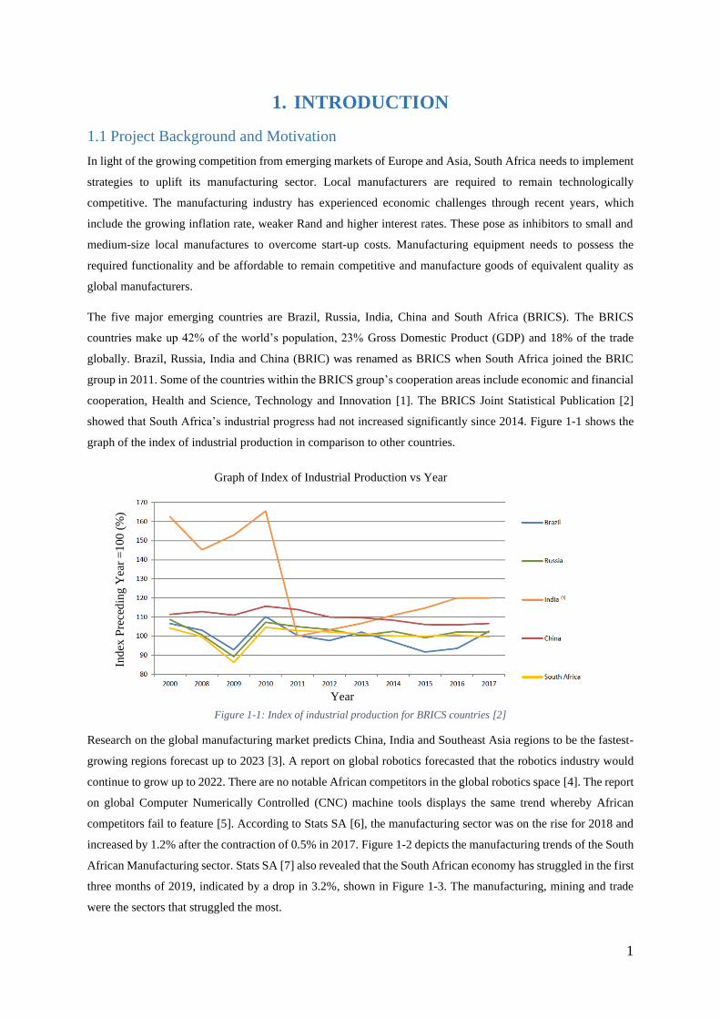
The five major emerging countries are Brazil, Russia, India, China and South Africa (BRICS). The BRICS
countries make up 42% of the world’s population, 23% Gross Domestic Product (GDP) and 18% of the trade
globally. Brazil, Russia, India and China (BRIC) was renamed as BRICS when South Africa joined the BRIC
group in 2011. Some of the countries within the BRICS group’s cooperation areas include economic and financial
cooperation, Health and Science, Technology and Innovation [1]. The BRICS Joint Statistical Publication [2]
showed that South Africa’s industrial progress had not increased significantly since 2014. Figure 1-1 shows the
graph of the index of industrial production in comparison to other countries.
Figure 1-1: Index of industrial production for BRICS countries [2]
Research on the global manufacturing market predicts China, India and Southeast Asia regions to be the fastest-
growing regions forecast up to 2023 [3]. A report on global robotics forecasted that the robotics industry would
continue to grow up to 2022. There are no notable African competitors in the global robotics space [4]. The report
on global Computer Numerically Controlled (CNC) machine tools displays the same trend whereby African
competitors fail to feature [5]. According to Stats SA [6], the manufacturing sector was on the rise for 2018 and
increased by 1.2% after the contraction of 0.5% in 2017. Figure 1-2 depicts the manufacturing trends of the South
African Manufacturing sector. Stats SA [7] also revealed that the South African economy has struggled in the first
three months of 2019, indicated by a drop in 3.2%, shown in Figure 1-3. The manufacturing, mining and trade
were the sectors that struggled the most.
Year
Graph of Index of Industrial Production vs Year
Ind
ex P
rece
din
g Y
ear
=1
00
(%
)

2
Figure 1-2: South African Manufacturing Statistics [6]
Figure 1-3: Industry growth rates for the first quarter of 2019 [7]
Robotic platforms have been adopted to assist in manufacturing tasks to lower lead times and produce high quality
goods. These platforms aid the economy. Importing manufacturing equipment, coupled with their large costs and
the cost of starting up a manufacturing plant, inhibits the start-up of small and medium-size local manufacturers.
Cost-effective robotic platforms can assist current and potential small and medium-size local manufacturers to aid
the economy. Pandilov and Dukovski [8] documented the variety of tasks that serial robots and Parallel Kinematic
Manipulators (PKMs) can accomplish. Serial robots can perform welding, palletising, assembly line applications,
packaging and part handling. PKMs can be employed for fine positioning, pick and place applications, machining,
motion platforms and surgical applications [8-11].
3
A PKM is a robotic platform with two or more closed-loop kinematic chains. Each kinematic chain connects to a
common base and end effector. PKMs possess high mechanical rigidity, the ability for fine positioning of the end
effector, high payload to weight ratio and there is non-cumulative error propagation. The drawbacks of PKMs are
a relatively small workspace, complex kinematic analyses and sophisticated calibration methods [10, 12]. Serial
robots possess an open-loop kinematic chain. They possess a large workspace, high workspace to robot size ratio
and simple forward kinematic analysis. However, they suffer from joint error propagation, relatively low
mechanical stiffness and are susceptible to vibrations [13, 14]. Each type of robotic platform has its own merits
and drawbacks. This research proposed the concept of using a novel PKM to validate positioning, machining, part
handling and sorting applications. Industrial companies could adopt a large-scale version of the PKM.
1.2 Existing Research and Research Gap
PKMs have received growing attention in past decades and their high payload to weight ratio has been attractive
to researchers [8]. The concept of robot machining originated in the early 1990s to accomplish CNC machine-
type tasks [15]. CNC machines perform machining applications in the automotive and aerospace industries. They
are capable of machining with high precision. However, the drawbacks of these machines are that they are large,
heavy and expensive [16, 17]. Affordable industrial robots for machining applications are currently not realised
in the industry.
In comparison to CNC machines, industrial robots possess a low capital investment and the flexibility to be applied
to various applications [18]. The flexibility and reusability of robotic systems make them a viable alternative for
various tasks [14]. Robotic systems possess a better workspace to installation space ratio than CNC machines [8].
According to Brüning et al. [18] and Karim and Verli [17], industrial robots have high economic potential for
machining applications in the automotive and aerospace industries.
There is a research gap in the development of affordable robotic manufacturing systems to assist small to medium
size companies to enter the South African market. The proposed robotic system served to validate part handing,
sorting, general positioning and robotic machining applications. A large-scale, more robust architecture could
perform these tasks as industrial applications. Some of the industries that could benefit from this research are the
automotive, mining and aerospace industries. Research suggests that a PKM can be developed to suit specific user
workspace requirements, therefore, reducing costs and eliminating unused machine functionality [19]. This
research explored different joint combinations to achieve a higher range of rotation. These joint combinations
could provide additional stiffness and tighter machine tolerances.
The novel 5 Degree of Freedom (DOF) PKM explored the exclusive use of revolute and prismatic joints. A
desktop prototype was produced through Additive Manufacturing (AM) and was tested as a proof-of-concept. The
inverse kinematic analysis was solved which aided in the forward kinematics, singularity and workspace analyses.
1.3 Research Aim and Objectives
Aim
This research aimed to design and investigate a novel 5-DOF parallel kinematic robotic system that can be used
to validate machining, part handling, sorting and general positioning applications.

4
Project Objectives
1. Research and establish insights in parallel kinematic robotic systems.
2. Synthesise a novel PKM that possesses 5 DOFs through an established methodology.
3. Research, develop and simulate the kinematic models for the robotic platform.
4. Research and simulate the workspace and identify singularities.
5. Research, design and construct a desktop prototype.
6. Research, design and implement a suitable electronic system to automate the mechanical platform.
7. Research and develop experiments and methods of data collection to verify the performance of different
types of movements that validate the application in machining, part handling, sorting and general
positioning tasks.
1.4 Methodology
The research conducted followed the steps listed below:
• Perform research on parallel kinematic robotic systems.
• Research various types of PKMs and establish directions for machine synthesis.
• Perform the mechanical design concurrently with the design for workspace and kinematic modelling.
• Identify the physical limitations of the machine to establish its workspace and singularities.
• Construct a desktop prototype through additive manufacturing.
• Research, design and implement a suitable electronic and software system.
• Research, design, plan and execute a series of experiments and tests that verify the kinematic models and
payload characteristics.
• Report on the findings of this research in an MSc. dissertation and in conference and journal publications.
1.5 The Scientific Contribution of Dissertation
This research study made the following contributions:
i. A novel 5-DOF PKM with a higher range of rotation than most 5-DOF and 6-DOF PKMs.
ii. A novel inverse kinematic model also used to develop the forward kinematic equations and perform the
workspace analyses.
iii. An Optical Computer Mouse (OCM) used as a low-cost position sensor and its implementation.
iv. Insights on the kinematics, workspace and isotropic characteristics of the robotic platform.
Research Question: Can a novel PKM be developed for 3 translational and 2 rotational DOFs to validate part
handing, sorting, general positioning and robotic machining capabilities?
1.6 Overview of Dissertation
Chapter 1: Introduces the reader to the background of this research, motivation for the study, the resulting
scientific contributions, and methodology. This chapter also presented the aim and objectives.
Chapter 2: Presents the comparison between serial and parallel kinematic manipulators and a review on PKMs.
A critical reflection of the literature is presented.

5
Chapter 3: Documents the concept generation of the PKM and a Quality Function Deployment (QFD) analysis.
Chapter 4: Presents the design methodology and mechanical design of the robotic platform.
Chapter 5: Presents the inverse and forward kinematic analyses.
Chapter 6: Presents the singularities and the workspace analyses.
Chapter 7: This chapter discusses the selection of electronic components and software systems.
Chapter 8: Presents the system performance and testing of the PKM under different conditions of motion.
Chapter 9: This chapter discusses the design and performance of the PKM, considering the aim and objectives.
Chapter 10: Concludes the dissertation with key insights, limitations, recommendations and future work.
1.7 Chapter Summary
This chapter introduced the reader to the manufacturing challenges faced by South Africa. This chapter also
presented the motivation for this research, a background to robotic platforms and a research gap. The aim and
objectives of this research and the contribution of the study were presented. The methodology was presented
before an overview of the dissertation was presented. The next chapter presents the literature review of the study.
Manufacturing challenges and trends are discussed. The relevance of this research is placed within the context of
Industry 4.0. A review of different DOF PKMs is presented and insights are discussed regarding their novelties,
merits, challenges and applications.

6
2. LITERATURE REVIEW
2.1 Current Manufacturing Challenges and Trends
Industry 4.0 is defined as follows: “a collective term for technologies and concepts of value chain organisation
which draws together Cyber-Physical Systems, the Internet of Things (IoT), and the Internet of Services” [20].
The objective of Industry 4.0 is to, therefore, drive fundamental improvements to industrial processes centred on
manufacturing facilities, engineering, material handling and supply chain and life cycle management. The aim is
to create a “Smart Factory” through the collaboration between the IoT and Cyber-Physical Systems [21]. Figure
2-1 shows the evolution of the various industrial revolutions.
Figure 2-1: Depiction of the industrial revolutions [22]
The IoT encapsulates the following necessities: flexibility, adaptability, the efficiency of people and processes,
quicker response time to decision making, customization, integration of business partners and value processes
concerning cyber-physical systems [23]. The IoT mainly focusses on the inter-networking of devices and
machines. These, in turn, must possess communication capability. As the rate of communication and information
exchange increases, this directly improves efficiencies in a manufacturing environment.
Cyber-Physical Systems makes use of advanced technologies that manage interconnected systems, which are its
physical assets and computational capabilities [24]. These interconnected systems are a family of software,
sensors, machines, workpieces, other physical objects and the communication system which monitors physical
processes, creates a virtual reality and can make decentralised decisions in order to exhibit intelligent behaviour.
This intelligent behaviour is meant to occur whilst machines communicate with each other, humans and a
centralized communication system [20].
Figure 2-2 depicts the three levels that are required for a Cyber-Physical System to exist. The physical objects can
store documents and knowledge about themselves on a network, which could be a cloud-based network. This
information can be updated and augmented in order to create another identity for them on the network as data
objects. The data objects are searchable and can be explored and analysed. The data objects form a knowledge
base for different applications. Algorithms make use of this knowledge base and optimize the autonomy and

7
intelligent behaviour exhibited by the physical objects. Through these algorithms and the availability of bulk
information, services that were previously not possible can now be developed [22].
Figure 2-2: The three levels required to form a CPS [22]
The emergence of Industry 4.0 demands that manufacturing industries incorporate new technologies and
methodologies in order to stay competitive. Through the exploitation of internet capabilities and embedded
systems, countries like Germany have already started adopting this paradigm [20, 22]. The adoption of the
paradigm has the potential of creating a variety of new products and market share will soon be gained by those
that possess the best technological competitiveness. South Africa cannot neglect to adapt to this change or it risks
falling further behind in manufacturing competitiveness.
Robotic platforms can provide the needed flexibility for manufacturing and assembly lines and whilst innovation
can lead to more cost-effective robotic platform solutions to address the needs of the South African manufacturing
sector. Manufacturing environments can use serial, parallel and hybrid robotic platforms with the serial
architecture currently the most widely adopted [8]. This research provides a novel robotic platform to validate
industrial applications. Interconnected systems can be implemented to further develop the PKM into an Industry
4.0 applicable robotic system.
2.2 Machine Architectures
2.2.1 Serial Kinematic Architectures
The serial robot is an open-loop kinematic chain characterized by links connected in series through one type or
different types of joints [25]. A serial robot has a fixed base and an end effector attached to the last link in the
chain. The type of end effector employed is dependent on the application. Serial manipulators have an industrial
presence, especially in factories. Some applications include handling of radioactive elements, automotive
assembly lines, space exploration, welding and palletizing [25] [8].

8
The advantages of the serial manipulator are its large workspace to installation ratio, simple calibration, easy
forward kinematic analysis and modelling and solving its dynamics characteristics is relatively simple [8].
Drawbacks of the serial architecture include propagation of joint errors, low stiffness, high inertia, low payload
to weight ratio and low speed and acceleration [8]. Figure 2-3 depicts a serial robot developed by FANUC
corporation of Japan [26].
Figure 2-3: A serial robot developed by FANUC corporation of Japan [26]
In light of extending the functionality of serial robots, researchers have explored overcoming its low stiffness and
complex programming characteristics. The serial robot has a high workspace to installation space ratio. Wang et
al. [13] developed a feed-forward compensation scheme to compensate for robot deformation induced by
machining forces. The machine stiffness was improved and produced a better surface finish to a milled aluminium
block. Figure 2-4 depicts the serial robot used for the investigation. Karim and Verl [17] and Chen and Dong [15]
surveyed recent advancements in using serial robots in high stiffness applications with a focus on trajectory
planning, vibration/chatter analysis, advanced and flexible programming and the optimisation of mechanical
stiffness.
Figure 2-4: Stiffness testing of a serial robot [13].
Schneider et al. [14] researched and developed a position control system for a serial robot for machining using an
optical measurement system. Schneider et al. [27] proceeded to combine advanced programming and simulation

9
to create an ideal path for the robot under machining forces. Domroes et al. [28] developed a flexible programming
concept, which enabled the robot to mill water pump impellers autonomously. The flexible programming concept
enabled this to occur along a dynamically adapted path. This innovation enhanced the quality of robotic machined
components and improved productivity. Kubela et al. [29] proposed an online controller to compensate for
accuracy errors in KUKA serial robots due to backlash from drive reversion. The concept of an online controller
was validated and improved the system with almost no additional cost.
Klimchik et al. [30] analysed the modelling of manipulator stiffness and estimation of the cutting force. The
method was used to rank the performance of available industrial robots concerning several machining tasks.
Research conducted by Dumas et al. [31] evaluated the joint stiffness values for translational and rotational
displacements of the robot’s end effector for a specified force and torque. The research aimed to optimize
machining operations and assist in motion planning. Zargarbashi et al. [32] researched posture optimization
through the development of a performance index. The performance index evaluated the torque of the actuators
and the joint rates in accomplishing a specified robot posture during machining. A study performed by Lin et al.
[33] examined the posture optimization of industrial robots in order to reduce machining errors. Researchers agree
that the mechanical properties of serial robots limit the accuracy and efficiency achievable for high stiffness
applications such as robotic machining applications [13, 15, 27, 28, 30, 33, 34].
2.2.2 Parallel Kinematic Architectures
A PKM is a mechanism that possesses at least two independent closed-loop kinematic chains. Each closed-loop
kinematic chain is attached to a fixed platform (base) and an end effector [35]. PMKs find its niche in automated
manufacturing systems, motion simulators, surveillance, positioning, machining and pick and place applications
[8]. PKMs can either move spatially or be restricted to move along a plane permitting rotation about the axis
normal to the plane. Figure 2-5 (a) shows a spatial 6-DOF PKM for fine positioning applications possessing 3
translational and 3 rotational DOFs. Figure 2-5 (b) depicts a planar PKM with revolute joints [35].
Figure 2-5: Different architectural designs of PKMs [8, 35].
a. PKMs used for fine positioning applications [8].
b. The 3RRR PKM with planar motion capabilities [35].
PKM architectures reduce the effect of cumulative joint positioning errors by averaging errors, thus providing
high accuracy and repeatability. Other advantages are high speed and acceleration, low inertia of moving masses
for certain architectural types and a relatively high payload to weight ratio [36]. PKMs possess a limited range of
a. b.

10
motion and small workspace for a relatively high number of actuators. Since the joints are interdependent,
mathematical modelling becomes complex concerning the forward kinematic analysis [36]. Calibration can also
be complicated [8]. For these reasons, parallel and serial manipulators find relevance in different types of
applications although not limited to those applications.
There have been successful PKMs that have been adopted by industry which includes the Stewart-Gough Platform
developed by Dr. Eric Gough [37]. Its initial application was for testing the properties of tyres under different
loads [37]. Flight simulators also use the Stewart-Gough Platform. The Delta robot was developed by Clavel [38]
which used the concept of parallelograms in its architecture; Bosch GmbH commercialised this robot for the
packaging industry [8]. The flex-picker was developed and commercialised by ABB. The Delta robot provided a
basis for the design of the flex-picker [38]. The flex-picker performed rapid pick and place applications.
Concerning machining applications, a significant study was the free leg hexapod by researchers such as Olarra et
al. [19] for miniature machining applications. The different foot configurations altered the workspace, which was
aided by machine programming. This allowed the optimization of foot configurations for the intended application.
Glavonjic et al. [39] performed research, design and construction of a desktop 3-axis parallel kinematic milling
machine. The PKM was an educational desktop model. The PKM machined soft material and the concept was
proven. The machine, however, could not be commercialised. Figure 2-6 illustrates the prototype.
Figure 2-6: Desktop 3 DOF parallel kinematic milling machine [39]
The Okuma’s Cosmo Centre PM600 and the FANUC F-200iB are commercially available platforms. The Cosmo
Centre PM600 performs machining applications and the FANUC F-200iB can accomplish positioning and
machining tasks [8, 40, 41]. These platforms are described further in Section 2.3. Metrom Mechatronische
Maschinen GmbH and Krause and Mauser have also produced milling machining centres which are large [8, 42].
The Quickstep, developed by Krause and Mauser, is shown in Figure 2-7 [8].

11
Figure 2-7: The Quickstep machining centre and the kinematic structure of the manipulator [8]
2.2.3 Comparative Analysis of Serial and Parallel Architectures
Table 2-1 depicts a comparative analysis between serial and parallel kinematic manipulators [8].
Table 2-1: Comparison between serial and parallel kinematics
Feature Serial Kinematic Manipulator Parallel Kinematic Manipulator
Workspace Large Small
Solving the forward kinematics Easy Difficult
Solving the inverse kinematics Difficult Easy
Position error Accumulates Averages
Force error Averages Accumulates
Maximum force Minimum actuator force limits the
maximum force
All actuator forces summed
together
Stiffness Low High
Dynamics characteristics Poor. Worsens with increased size High
Modelling and solving
dynamics
Relatively simple Complex
Inertia High Low
Payload to weight ratio Low High
Speed and acceleration Low High
Accuracy Low High
Calibration Simple Complex
Workspace to robot size ratio High Low

12
2.2.4 Hybrid Architectures
Open and closed-loop kinematic chains characterize hybrid architectures. These mechanisms may be connected
in series, known as a conventional hybrid structure, or in parallel, known as a cooperative structure. There are 3
types of conventional hybrid structures: parallel-parallel type, serial-parallel type or parallel-serial type [43].
Hybrid architectures find their niche in machining applications such as metal cutting, polishing, woodworking
and spot welding. Hybrid mechanisms are also capable of holding a laser and saw cutting tools. Automobile and
aerospace manufacturers make use of this type of machine architecture for component assembling, welding,
fabrication of turbine blades, impellers, high-speed milling and other items that require contouring [8, 44].
The hybrid manipulator was designed and developed by Karl-Erik Neumann in 1987. Figure 2-8 (a) depicts the
patent known as the Tricept robot. Neos Robotics, Inc commercialised it. It possessed 3 degrees of freedom (2
rotational and 1 translational degree). The initial obstacle for the design was that the computational power required
for intended functionality was unavailable. Comau Pico produced the first multiprocessor controller and overcame
the challenge of computational power. The controller and open architecture made it possible to process the
complex kinematics exhibited by this mechanism. The hybrid architecture performed machining applications.
Figure 2-8 (b) depicts the Tricept 805. It combines the flexibility from serial robots and the stiffness of a parallel
robotic system [8].
Figure 2-8: The hybrid Tricept-type PKMs [8]
a. The patented design of the Tricept by Karl-Erik Neumann comprised of a parallel architecture with a
serial architecture end effector [8].
b. The Tricept 805 comprised of a parallel architecture with a serial architecture end effector [8].
In 2002, ABB and SMT Tricept launched the IRB 940. The IRB 940 performed heavy-duty cleaning and pre-
machining of aluminium parts [8]. The Trivariant hybrid structure was commercialised and formed part of the
HSC milling centre. Like the Tricept, the Trivariant possesses 5 DOFs [44, 45]. The Exechon machining centre
is a hybrid architecture with 5 DOFs. It has an over-constrained kinematic structure with eight links and nine
joints [46, 47]. It has excellent potential in drilling applications with high flexibility. Siemens [48] developed the
controller for the system. Figure 2-9 displays the Exechon.
Dörries Scharmann Technologie GmbH developed the ECOSPEED and ECOLINER machining centres which
incorporate the Sprint Z3 tool head. The tool head is a parallel kinematic tool head that can move in translationally
a. b.

13
in one direction and tilt in all directions. The serial component is incorporated through a planar cross slide. This
hybrid machining centre finds its applications in high-speed machining of large aluminium structural components.
In the aerospace automotive and tool and die industry, it is useful in the production of small to medium size
components [40]. The VERNE Machine was developed by Fatronik for IRCCyN. It consists of a parallel module
which provides the translational movement. A tilting worktable imparts rotation about two orthogonal axes, thus
classified as hybrid architecture. It machined complex parts especially in the moulding industry [49]. The
TriCenter machine was based on the kinematics of the Tricept and aimed to improve rigidity. Its architecture was
similar to the Tricept whereby it possessed a 3-DOF parallel manipulator with a 2 axis serial milling head [40].
Figure 2-9: Architectural design of the Exechon [48]
Hybrid architectures, therefore, seek to retain the large workspace and high dexterity of serial manipulators and
high payload to weight ratio and high stiffness of PKMs while minimizing the disadvantages of both [43]. Despite
the advantages of hybrid kinematic systems, there is no systematic method that enables the design of a hybrid
kinematic system without having to perform a separate synthesis for each of the mechanisms that would be
attached. This drawback was examined by Campos et al. [43] but the method presented does not use computer
algorithms, which may result in chain isomorphisms. According to Harib et al. [46], a comprehensive study and
understanding of the kinematics, dynamics and design of hybrid architectures are still lacking. The investigation
of an exclusive serial robot or PKM leads to more straightforward kinematic analyses and programming. The
PKM architecture possesses attractive stiffness characteristics and a high payload to weight ratio is presented in
Section 2.3.
2.3 Review of Parallel Kinematic Architectures
2.3.1 Two DOF Systems
Duan et al. [50] developed a 2-DOF spherical PKM. It possessed two rotational DOFs and could be used for
vibration isolation, precision manipulation applications and as a 2-DOF orientation and force/torque sensor.
Figure 2-10 (a) illustrates the prototype. Qu et al. [51] researched a piezo-driven 2-DOF PKM for high precision
alignment applications as shown in Figure 2-10 (b). The PKM found relevance in orientation adjustment to ensure

14
alignment between two flat surfaces. The design used flexure-hinge based mechanisms and piezoelectric stack
actuators. A resolution of 1µrad was achieved. Bozorgi et al. [52] performed the design, development, dynamic
analysis and control for a 2-DOF spherical PKM. A robust algorithm for dynamic modelling was proposed and
was validated by the end effector following the prescribed trajectory. Lagrangian and Newtonian approaches were
used.
Reconfiguration analysis was performed by Kong [53] on a 2-DOF 3-4R PKM. The robotic platform was found
to possess 14 different operation modes while using the minimum number of actuated joints. Yang et al. [54]
proposed a modified robust control system for a 2-DOF PKM with planar translation motion. Yang et al. [54]
designed the diamond-shaped PKM for high speed and high precision part handling and assembly. Experimental
results validated the modified control system. The control method produced more accurate trajectories in
comparison to using traditional potential difference methods. Niu et al. [55] produced a novel 2-DOF PKM with
rotational DOFs. The PKM was designed with uncoupled and isotropic movements that possessed a larger
workspace, simple mathematical analysis, ease of control, high stiffness and dexterity. Applications include
aiming applications such as radar scanners, telescopes and cameras.
2-DOF PKMs exhibit exclusive rotation or translation of the end effector. 2-DOF PKMs are designed for a specific
category of applications. The flexibility and reusability of 2-DOF PKMs are limited. 2-DOF PKMs are cost-
effective are characterized by more straightforward mathematical analyses. They do, however, lack the
mechanical rigidity of a PKM possessing more legs. 2-DOF PKMs have not been widely adopted by industry.
High precision positional and rotational applications are well suited to 2-DOF PKMs due to the smaller
workspaces. High speed planar applications can be accomplished by 2-DOF PKMs. Greater depth of analysis,
regarding aspects such workspace and singularities, on 2-DOF PKMs are aided by their simpler mathematical
analyses.
Figure 2-10: Examples of 2-DOF PKMs [50, 51]
a. The spherical PKM developed by Duan et al. [50].
b. The piezo-driven, high precision PKM [51].
a. b.

15
2.3.2 Three DOF Systems
A biologically-inspired PKM, producing realistic eye movements, was developed by Bang et al. [56]. The
prototype was an improvement made to the Agile Eye developed by Gosselin and Hamel in terms of encasing the
PKM behind a layer of a humanoid face [56]. The PKM possessed only rotational movement of the end effector.
The Agile Wrist was also derived from the Agile Eye and was altered by using cylindrical joints as investigated
by Al-Widyan et al. [57]. The cylindrical joint was employed to alleviate manufacturing errors for spherical
PKMs. The PKM was designed to hold and orient a tool for shot-peening applications as is illustrated in Figure
2-11 (a). A notable 3-DOF PKM, called the Orthoglide, was developed by Chablat and Wenger [58] for exclusive
translational motion. The Orthoglide had the potential to be used for machining applications. Dahmouche et al.
[59] further investigated the Orthoglide. The purpose of their investigation was to determine if high-speed vision-
based computed torque control for dynamic control. The method was successfully employed and could be used
for robots that experience flexibility and backlash.
Liu and Kim [60] proposed a novel 3-DOF spatial PKM capable of large rotations of the end effector. The PKM
possessed 1 rotational and 2 translational DOFs. The footpoints were actuated and only single DOF joints were
used. The PKM explored the ease of assembly and disassembly through magnetic joints. Carbonari et al. [61]
designed a novel reconfigurable 3-DOF PKM. Metamorphic universal joints imparted the reconfigurability into
the PKM. The end effector could achieve either pure translation or pure rotation. Singularities were shared for the
different end effector motion cases and in the space of the actuation parameters. Nurahmi and Gan [62] also
explored the notion of a metamorphic 3-DOF PKM which used reconfigurable revolute joints located at the base
of the device. The end effector of this PKM exhibited operation modes of 3-DOF coupled rotations, 3-DOF planar
motion and 1 translation with 2 rotation movement. Figure 2-11 (b) illustrates the PKM.
Ahangar et al. [63] designed a 3-DOF delta PKM with 1-DOF redundancy attached to its base. The purpose of the
investigation was to save time and energy saving for pick and place applications along a conveyor. Al-Naimi et
al. [64] used machine vision in the development of a pick and place PKM for industrial applications. A novel
collision-free workspace method was explored for a 3-DOF delta PKM by Ataei et al. [65]. Kinetostatic indices
were used to measure the performance of the PKM. The novel algorithm was successful and can be used for path
planning. Other delta type PKMs were explored by various authors [66-68]. These investigations included using
a system of cams with a single drive [66], kinematic sensitivity evaluation [67] and applications in endonasal
surgery [68]. Arian et al. [69] investigated the dynamic characteristics of a planar 3-DOF PKM. A novel geometric
approached was used to solve the inverse kinematic models. The dynamic rigid-body model developed reduced
computation time by 58%.
3-DOF PKMs can exhibit 2 translation and 1 rotation, 1 translation and 2 rotations, pure translations or pure
rotations. The different combinations of translational and rotational DOFs allows 3-DOF PKMs to be employed
for a wider range of applications than 2-DOF PKMs. The 3-DOF class of PKM exhibits large differences in
appearance due to the nature of joint combinations and architectural layout. The delta and spatial type of PKMs
are most widely researched with the delta-type PKMs having an industrial presence. Sorting tasks are one of the
most common industrial application of 3-DOF PKMs. Many platforms require future work before being
implemented for industrial applications.

16
Figure 2-11: Examples of 3-DOF PKMs [57, 62]
a. The spherical PKM developed for shot peening applications [57].
b. The metamorphic 3-DOF PKM that was developed by Nurahmi and Gan [62].
2.3.3 Four DOF Systems
Niche applications of 4-DOF PKMs are packaging, picking, packing and palletizing tasks. Reymond Clavel
investigated the use of parallelograms to create a PKM that possessed one rotational and three translational DOFs.
A link directly connected from base to the end effector provides the rotational degree of freedom. His patent was
known as the Delta robot. This design was useful for pick and place applications [8, 70]. SIG Pack systems (part
of Bosch Packaging Technology division) and ABB Automation commercialised the Delta robot. Their products,
are known as the C33/CE33 Delta robots and the IRB 340 Flex Picker Robot, are shown in Figure 2-12 (a),
respectively [8].
Rasoulzadeh and Masouleh [71] investigated singularity configurations analysis using Grassmam-Cayley
Algebra. Kang et al. [72] investigated the kinematic modelling, analysis and load distribution algorithm of a 4-
DOF PKM that was redundantly actuated. Singularity analysis was performed on a novel surgical PKM by
Khalifa et al. [73]. Mohammadi et al. [74] explored the concept of kinematics concerning modelling and weighted
kinematic sensitivity. Screw theory is generally used to assist when obtaining the Jacobian matrix structure [71-
73].
A simulation study of a Delta robot was conducted by Azmoun et al. [75], which used a Proportional-Integral-
Derivative (PID) and Sliding-Mode controller based on the inverse kinematic analysis. Akhbari et al. [76]
developed a novel asymmetrical 4-DOF delta PKM for milling applications, as depicted in Figure 2-12 (b). The
results showed that the asymmetric configuration and different link lengths improved the singularity avoidance
and dexterity. Apostolescu and Ionaşcu [77] developed a new delta 4-DOF PKM for pick and place and stacking
tasks. The PKM was able to detect new objects in its workspace and rotate objects irrespective of initial
orientation. Control and vision of a 4-DOF PKM were investigated by Rouhollahi et al. [78] to improve pick and
place tasks from a conveyor belt. Physical experimentation validated the use of the proposed system.
The most common topology discovered for 4-DOF parallel manipulators is the delta structure with 3 translational
and 1 rotational DOFs. Some 4-DOF PKMs have been implemented industrially exclusively for pick and place
applications. 4-DOF PKMs are generally larger than 2-DOF and 3-DOF PKMs hence they possess a larger
a. b.

17
workspace. Recently, 4-DOF PKMs have been employed for AM applications. Actuation of 4-DOF PKMs are
generally in the form of a rotational input thus the motors are situated on the base. The low inertia allows fast
movements of the end effector but this architectural type suffers from poor mechanical rigidity. Actuation
redundancy has been explored for 4-DOF PKMs which aimed to reduce singularity challenges.
Figure 2-12: Examples of 4-DOF PKMs [8, 76]
a. The ABB IRB 340 Flex Picker [8].
b. The asymmetric delta robot developed by Akhbari et al [76].
2.3.4 Five DOF Systems
Early research mainly concentrated on 6-DOF hexapod type PKMs however, 6-DOF PKMs have a relatively
small workspace. Some industrial applications do not require 6 DOFs. Therefore, it's beneficial to study PKMs
with fewer than 6-DOFs. Advantages of PKMs that possess fewer than 6-DOFs include a more straightforward
mechanical design, fewer components, thus more cost-effective, larger workspace and a simpler controller can be
used. Except for the delta type architecture for 4-DOF PKMs, there are relatively few papers on 4-DOF and 5-
DOF PKMs. There exist a difficulty to design 4-DOF and 5-DOF PKMS with identical limb structure [79]. Fang
and Tsai [79] presented a systematic structure synthesis of a class of 4-DOF and 5-DOF PKMs that possess
identical limb structure. Various joint and layout combinations were enumerated, inclusive of the number of DOFs
permitted. Hairong et al. [80] used screw theory to analyse the motion screw and constraint screw of the limbs
and end effector, respectively. Screw theory was used to create a synthesis procedure for the development of a
symmetrical 5-DOF PKM. This method was validated through simulations done on PKMs possessing 3 rotational
and 2 translational DOFs.
Li et al. [81] investigated the type synthesis of a 3 rotational and 2 translational (3R2T) 5-DOF parallel
manipulator, which makes use of Lie Group of Displacements. Fourteen novel architectures are revealed for the
3R2T 5-DOF parallel manipulator. This method can be used for the enumeration of lower mobility PKMs. Fiore
et al. [82] performed a dimensional synthesis of a 5-DOF parallel manipulator for AM applications. The
parameters were optimized using a genetic algorithm to generate the workspace. The control system was outlined.
The PKM could achieve larger movements that were not feasible with general AM machines.
Guo et al. [83] developed a ship active vibration isolation system, which was based on a novel 5-DOF PKM. PID
control and force-position redundant control was employed. ADAMS®-MATLAB Simulink® simulations were
a. b.

18
conducted to improve the control of the PKM. The dynamic model was obtained through the Lagrange method
and the control system based on ship motion. A 5-DOF Parallel Machine Tool (PMT) developed by Zheng et al.
[84], possessed 3 translational and 2 rotational DOFs. The PKM had 1 passive and 5 active limbs. Multi-axis
simultaneous control was investigated in detail in order to control the path traced by the machine tool. Course
interpolations algorithms and mapping transformations were implemented. The PKM accomplished 5-axis
machining with high position accuracy and low vibrations.
Further work conducted on the PMT involved a motion control algorithm investigated by Cheng et al. [85]. A
concise motion control algorithm was deduced from the Euler angles of the end effector and was developed in
conjunction with the inverse kinematic solution. This algorithm was successfully applied to the PMT and results
showed that the positional and repeatable errors were reduced. Figure 2-13 (a) depicts the PMT. Ersoy et al. [86]
developed a 5-DOF PKM for beating heart surgery. It was designed as a lightweight PKM. The purpose of the
PKM was to track the heartbeat motion during a coronary artery bypass procedure. This unique 5-DOF PKM uses
two separate subsystems to position the end effector accurately. It possessed a 3-DOF remote stage and a 2-DOF
fixed stage. Simulations and experimentations showed that the heartbeat motion data was tracked with a 0.66mm
error.
A novel hybrid 5-DOF PKM, named the T5, was designed for machining applications by Song et al. [87], which
comprised of 2 PKM subsystems in series. A flow path is presented to synthesise a PKM which was accomplished
in 4 steps. The design of this PKM was patented and was intended for high precision machining applications on
large-scale structural aircraft components. Screw theory was applied for the kinematic analysis and a kinematic
performance index was defined. The research also presented multi-objective dimensional optimization using a
nondominated sorting genetic algorithm. The T5 was further explored by Sun et al. [88]. The authors addressed
the improvement of PKM geometric errors at the design stage through a design optimisation method. The research
aimed to minimize vibration and deformation through an electrodynamic optimization method. The geometric
errors were treated as parameter uncertainty. Figure 2-13 (b) illustrates the T5 PKM.
Qiu et al. [89] presented a method of Three-Dimensional (3D) modelling of a 5-DOF PKM possessing branched
chains. The PKM possessed 2 rotational and 3 translational DOFs. Concerning the branched chain, a notable
feature was the attachment of limbs to upright brackets and with the brackets themselves possessing additional
joints. Xiaolong et al. [90] proposed a 5-DOF PKM with redundant actuation as is illustrated in Figure 2-13 (c).
The PKM consisted of 4-SPS limbs and 2-RPS limbs. The PKM could perform 3 rotational and 2 translational
movements. The PKM had 4 limbs mounted symmetrically around its base and the 2-RPS joints were located
along a plane across on centre of the base. A notable feature was the restriction of one transitional DOF through
the arrangement of the revolute joints.
Zhu et al. [91] investigated the limb and actuation singularities of a fully symmetrical 5-DOF PKM which could
be used for simulating the motion of a spinal column. This is another 5-DOF PKM possessing 3 rotational and 2
translational DOFs. The singularity analysis was performed using screw theory and Grassmann geometry. The
PKM employed revolute joints, which passively restricted a translational DOF and is depicted in Figure 2-13 (d).
Liu et al. [92] developed a 5-DOF portable machining robot named DiaRoM for the processing of large structural
elements and remote maintenance on large equipment or components. The Grassmann Line Geometry and Line-

19
graphs were used to synthesise the design. Flexible 5-axis machining was achieved and with the ability to
transform between horizontal and vertical machining modes. Huang et al [93] developed a novel 5-DOF PKM
with 5 active legs and 1 passive leg. The passive leg was positioned at the center of a circular base and the PKM
was designed to be symmetrical. This PKM possessed 3 rotational and 2 translational DOFs. The inverse
kinematics, velocity and accelerations were validated through simulations. Metrom developed a 5-axis Pentapod
machine with a unique end effector design which allowed each of the 5 actuators to be attached to it by individual
revolute joints. The end effector achieved rotations of up to and including 90°. The workpiece was mounted on a
rotary work table, which imparted an additional DOF to the machining centre but did not affect the PKM structure.
A control strategy was implemented to take into account the movements of the rotary worktable [94].
5-DOF PKMs include numerous novel architectures and unique architectural layouts in comparison to other DOF
PKMs. The most common motion type of the end effector is 3 rotational and 2 translational DOFs. There are rare
instances of the PKM possessing 2 rotational and 3 translations DOFs. 5-DOF PKMs generally exist as hybrid
systems and there are examples of hybrid PKMs having some but little industrial presence [8]. Many experimental
5-DOF PKMs have been developed and many have only been analysed from a computational standpoint. Many
authors have not followed through with functional prototypes and the implementation of a 5-DOF pure PKM
system in the industry is lacking. The category of 5-DOF PKMs has received lesser attention relative to 3-DOF,
4-DOF and 6-DOF PKMs. Most 4-DOF PKMs possess the delta structure whilst most 6-DOF PKMs are exploited
for their high stiffness characteristics. 5-DOF PKMs can therefore utilise advantages of 4-DOF and 6-DOF PKMs
and be positioned to improve specific applications carried out by 4-DOF and 6-DOF PKMs.
Figure 2-13: Examples of 5-DOF PKMs [84, 88, 90, 91].
a. The PMT developed by Zheng et al. [84].
b. The T5 PKM machining system [88].
c. A redundant actuated 5-DOF PKM [90].
d. The PKM designed by Zhu et al. which makes exclusive use of revolute joints [91].
a. b.
c. d.

20
2.3.5 Six DOF Systems
6-DOF PKMs possess 3 rotational and 3 translational DOFs. Since it is trivial that all DOFs are permitted for 6-
DOF PKMs, research into these platforms include optimisation of PKM parameters, increasing workspace,
different calibration techniques, the potential use for new applications, improving control, methods of synthesis,
path planning, vibration analyses and a variety of other aspects. An early functional 6-DOF PKM was used for
the tyre testing which was developed by Gough and Figure 2-14 (a) [40] illustrates the platform. These types of
PKMs are referred to as “Hexapods” [40]. 6-DOF PKMs have been extensively researched and used for flight
simulation, micro-positioning, machining tools, light positioning in surgical labs and other many other
applications [8].
McCann and Dollar [95] developed a novel 6-PKM for grasping and dexterous spatial manipulation, as illustrated
in Figure 2-14 (b). A notable advantage was that the PKM could grasp objects with minimal sensing. The PKM
encountered challenges when grasping highly irregular objects. Spherical joints were used at the fingertip of the
robot to conform to firmly grasping objects passively but inaccurate grasping occurred that the limits of the
workspace for certain poses. Gonzalez and Asada [96] designed and developed a novel extendable PKM, called
the TSE, for use in aircraft assembly applications. The PKM was designed to reach high ceilings and to possess a
large workspace. The actuation of the robot’s foot points allowed a greater reach and the architectural layout could
be altered to suit the intended work envelope. The prototype could reach a maximum height of 1.62 meters. Figure
2-14 (c) illustrates the TSE PKM.
Stenzel et al. [97] used a 6-DOF parallel manipulator to simulate the motion characteristics of an emergency
vehicle for selected manoeuvres for obstacle avoidance. Forces were measured that act on a vehicle when driving
over a speed bump or during obstacle avoidance. The PKM was found to generate undesirable vibrations of higher
frequencies during testing. Becerra-Vargas et al. [98] explored a robust joint space control for a 6-DOF parallel
robot. This research sought to apply a robust inverse dynamic control with the control strategy based on the
Lyanpunov stability theory. Simulations validated that the joint control structure overcomes the real-time
implementation for the forward kinematics.
Trajectory planning was researched by Hasnaa and Mohammed [99]. The inverse kinematic model was
established for a 6-DOF PKM, named HEXA. The PKM was designed with rotary actuation of the joints instead
of prismatic joints and this allowed large workspaces to be achieved. The PKM was simulated in MATLAB® to
trace various trajectories. The kinematic models and path tracing were successful. Beiki and Irani-Rahaghi used
a nonlinear dynamic optimisation procedure for energy-efficient path planning. The energy consumption of the
actuators was analysed and the accuracy error of the end effector was investigated. The optimisation tool was
based on a finite element method. Simulation results based on dynamic modelling were performed in MATLAB®
and planning a minimum energy consumption path validated the method employed.

21
Figure 2-14: Examples of 6-DOF PKMs [40, 95, 96]
a. The tyre testing PKM developed by Gough [40].
b. A dexterous grasping PKM prototype [95].
c. The TSE PKM for aircraft assembly tasks [96].
Ding et al. [100] presented a statistical approach to reducing pose errors of a 6-DOF PKM. The structure of joint
clearance was analysed. The drawback encountered from this method was long computational time. Ghorbani and
Omurlu [101] investigated 3 different numerical methods to solve the coupled nonlinear forward kinematic
equations of a 6-DOF flight simulator PKM. The Adaptive-Network-based Fuzzy Inference System, Multilayer
Perceptron and Radial Base Function and Neural Network methods were implemented. Through experimentation,
the Adaptive-Network-based Fuzzy Inference System method proved to be the best of the 3 approaches. The
inverse kinematics and workspace analyses were conducted on a novel 6-PSS PKM by Xu et al. [102]. The design
explored the use of triangle rail trusses and sliders for the actuation of the footpoints. The largest workspace was
largely influenced by one of the angles of interest. The workspace was dependent on the actuator layout angle.
The feasibility was validated through SolidWorks® and MATLAB® simulations.
A novel 6-DOF PKM was designed by Harada and Angeles [103] which uses only 2 limbs but possessed kinematic
and actuation redundancy. The kinematic redundancy influenced singularity and collision avoidance which
generated a larger workspace. Actuation redundancy improved position accuracy. Simulations conducted on
MATLAB® demonstrated that collisions were avoided successfully while the PKM maintained its prescribed
position and orientation of the end effector.
The FANUC F-200iB, depicted in Figure 2-15 (a) is a successfully commercialised PKM used for welding,
loading, dispensing and material removal applications. The robot has exceptional rigidity and repeatability in
comparison to serial robots [8]. This robotic platform is expensive and not affordable to small and medium-size
manufacturing companies [41]. Barnfather et al. [11] investigated the machining capability of the FANUC F-
200iB to establish and minimise the position errors during non-cutting operations. The research was undertaken
to facilitate higher tolerance machining. The errors discovered were in the micron range and were attributed
mainly to the pose of the machine. The PKM could not machine to high tolerances due to static errors and
systematic errors were more dominant than random errors. It was suggested that a possible solution to reduce
positional errors is to perform in-situ process monitoring.
a. b. c.

22
OKUMA PM 600, shown in Figure 2-15 (b), was successfully commercialised and resembles the Stewart Platform
design. It was designed for machining aluminium components and dies and moulds that require less polishing.
The machine could perform high-speed machining and be suitable for continuous operation. The drawback of the
machine is that it is large and heavy [40]. Ibaraki et al. [104] expanded on the research of the OKUMA PM600
and performed kinematic calibration by circular tests to improve the contouring accuracy when performing
circular tasks. The calibration method was validated experimentally.
Figure 2-15: Commercialised 6-DOF PKMs [11, 40]
a. The FANUC F-200iB with a machining tool [11].
b. The OKUMA PM 600 [40].
6-DOF PKMs are exploited for their high stiffness characteristics since they possess 6 legs. 6-DOF PKMs
generally have an architectural layout similar to the hexapod layout. The high mechanical rigidity provided by 6-
DOF PKMs makes them attractive for, but not limited to, machining, general positioning and high vibration
applications. These reasons have led authors to focus attention more on applications and to improve PKM
performance indices. There was more novelty of machine architectural layout and limb configurations observed
in the 5-DOF PKMs in comparison to the 6-DOF PKMs. 6-DOF PKMs have been attractive thus, more research
was conducted on these platforms and there is more commercialisation of 6-DOF PKMs than 5-DOFs. The
rotational capability of 5-DOF PKMs is generally better than 6-DOF PKMs and the Pentapod PKM developed by
Metrom is an example [94].
The hexapod-type layout for 5-DOF and 6-DOF PKMs generally possess prismatic joints thus, the PKM has
higher inertia. The higher inertia of these PKMs makes them better suited for low-speed tasks but still possesses
the functionality to be used for pick and place operations that require a short distance to move parts. Workspace
can be designed to suit the application but the PKM’s kinematic, singularity and workspace analyses need to be
solved first. There is a tradeoff between large workspace and machine stiffness. Larger workspaces require all
motors to be mounted at footpoints but reduces mechanical rigidity. Mathematical kinematic and workspace
modelling is generally performed in MATLAB® while additional software such as ADAMS® and SolidWorks®
were used for motion analysis and 3D Computer-Aided Design (CAD) modelling respectively.
a. b.

23
2.3.6 Specifications of 5-DOF and 6-DOF PKMs
Novel architectures are developed to improve specific parameters of current PKMs. Research can also investigate
the optimisation of certain parameters of an existing PKM. It is then worth presenting the specifications of some
of the prominent and current PKMs for benchmarking. Table 2-2 presents the specifications of a sample of PKMs.
A comprehensive list of PKM specifications can be found in the research conducted by Weck and Staimer [94]
and details of some commercially realised PKMs were presented by Pandilov [40].
Table 2-2: Specifications of a sample of PKMs
PKM Workspace X*Y*Z
(mm)
Rotation (degrees) Accuracy Repeatability
Fanuc F-200iB [41] ±520 * ±510.93 *
437.27
Depends on end
effector mounting.
N/A ±0.1 mm
Hexabot [10] ±152.2 (X-Y) * 178 ±25 N/A 10 µm
OKUMA PM 600
[105, 106]
Ø600 (X-Y) * 400 ±25 5 µm N/A
Mikrolar P1500
[107]
Ø725 (X-Y) * 273 ±25 50 µm 25 µm
Mikrolar Hex-A-Jet
P3000 [108]
Ø1 219 (X-Y) * 508 ±15 (X, Y Axis)
±5 (Z Axis)
±0.05 mm 0.03 mm
Metrom Pentapod P
800 [94, 109]
Ø600 (X-Y) * 400 ±90 ±0.020 mm 0.003 mm
Hexact [94] 200*200*100 ±15 (X, Y Axis)
±5 (Z Axis)
±20 µm <5 µm
Hexapode 300 [94] 700*700*300 N/A 8 µm/300 mm ±1 µm
Geodetic G500 [94] 500*500*500 N/A ±25 µm ±5 µm
Giddings&Lewis
Variax [94]
700*700*750 ±25 12 µm N/A
The workspace is directly proportional to the length of linear actuators used however, the rotational range should
theoretically remain the same assuming all components are scaled by the same factor. There are a few 5-DOF and
6-DOF PKMs that exceed a rotational range of ±30°. Concerning 5-DOF PKMs that are parallel (not hybrid), only
the Metrom P800, Sena Eclipse and the Tekniker Seyanka PKMs included and exceeded a rotational range of
±30°. There is a niche for the development of 5-DOF PKMs with high rotational capabilities that exceed rotational
capabilities of 6-DOF PKMs to give them more industrial relevance. There is also a challenge to produce
affordable PKMs that are also lightweight and mobile.
2.4 Chapter Summary
This chapter presented the concept of Industry 4.0 and the relevance of this research within this context. Serial,
parallel and hybrid robotic architectures were investigated and a comparative analysis was performed on serial
and parallel kinematic architectures. A review of different DOF PKMs was researched regarding their novelties,

24
merits and challenges of each and their applications. Specifications of some 5-DOF and 6-DOF PKMs were
presented with the establishment of a research gap.
The literature suggested that 2-DOF PKMs exhibit either rotation or translation of the end effector. 2-DOF PKMs
are designed for specific applications, they are cost-effective and possess simpler mathematical analyses. 2-DOF
PKMs lack the mechanical rigidity and have not been widely adopted by industry. 3-DOF PKMs exhibit a
combination of translational and rotational DOFs and can be designed to possess only translations or rotations of
the end effector. The delta and spatial types are most commonly researched while many 3-DOF PKMs require
future work. The delta structure is the most common topology of 4-DOF PKMs and is used mainly for pick and
place applications. 4-DOF PKMs have been employed for AM applications. 4-DOF PKMs possess low inertia
permitting high-speed movements but lack mechanical rigidity.
5-DOF PKMs generally possess 3 rotational and 2 translational DOFs. 5-DOF PKMs commonly exist as hybrid
systems and hybrid PKMs having some industrial presence. Many experimental 5-DOF PKMs have been
developed but have not been commercialised. The category of 5-DOF PKMs has received lesser attention than
others. 6-DOF PKMs are exploited for their high stiffness characteristics and are generally similar in appearance
to the Hexapod-type layout. Some 6-DOF PKMs have been commercialised. The rotational capability of 5-DOF
PKMs are generally higher than 6-DOF PKMs and 5-DOF PKMs possesses more novelty than 6-DOF PKMs.
4-DOF PKMs possess larger workspaces than 5-DOF and 6-DOF PKMs. There is a tradeoff between large
workspace and machine stiffness.
The succeeding chapter discusses the PKM concept generation and selection. A sequential synthesis for the
architectural design of the PKM is presented. Insights of the machine synthesis are discussed. The architectural
design and PKM novelties are presented. A QFD analysis was performed to aid in the development of target
specifications. Potential customer requirements and their relationships to engineering metrics were reviewed. The
relationship between the different engineering metrics were investigated.

25
3. CONCEPT GENERATION AND SELECTION
3.1 Introduction
This chapter presents the synthesis methodology for the development of a novel PKM. Concepts and ideas from
Section 2.3 were explored to give insights into the development of a new joint. The architecture is described with
its novelties. A QFD process was used to develop target specifications and to understand the different relationships
within the design process.
3.2 Machine Synthesis
Figure 3-1 illustrates the synthesis of PKM topologies. Pandilov and Dukovski, and Weck [40, 94] described the
process. The systematic methodology was broken down into the following steps:
1. Joint selection and limb topology.
2. Selection of architectural type, DOFs and motors dedicated to each limb.
3. Configuration of joints on the base.
4. Configuration of joints on the end effector.
5. Direction of the applied force of the actuators.
6. The direction of the z-axis.
The subsections of Section 3.2 present the step by step synthesis methodology.
Figure 3-1: PKM synthesis [40]

26
3.2.1 Joint Selection and Limb Topology
A kinematic pair is established when two rigid links are coupled, resulting in restrained relative motion. Kinematic
pairs are classified as either a lower or an upper kinematic pair. A lower kinematic pair is established when two
rigid bodies maintain surface contact. An upper pair is restrained such that the two rigid bodies that keep a line or
point contact [35]. An example of an upper kinematic pair is a pair of gears. There are six types of lower kinematic
pairs, as listed below and categorized in terms of their DOFs [35]. Figure 3-2 depicts the different type of joints:
• Prismatic (P): Allows translation along 1 axis (1 DOF)
• Revolute (R): Allows paired elements to rotate concerning each other about 1 axis (1 DOF)
• Cylindrical (C): Allows translation and independent rotation about 1axis (2 DOFs)
• Helical (H): Allows translation and independent rotation about 1axis (2 DOFs)
• Spherical (S): Allows paired elements to rotate concerning each other about 3 axes (3 DOFs)
• Planar (E): Allows translation along 2 axes and rotation about 1 axis (normal to the plane) (3 DOFs)
Figure 3-2: The different types of joints [35]
A Universal joint (U) combines two revolute joints to permit rotation about two axes that are perpendicular to
each other. This joint allows 2 rotational DOFs as shown in Figure 3-3 (a). The Parallelogram (Pa) joint is
comprised of 4 links and adds to the stability of the limb structure. The Pa joint is illustrated in Figure 3-3 (b).
The Pa joint allows 1 DOF.
Figure 3-3: An example of a universal joint and a parallelogram joint.
a. A Universal (U) joint [110].
b. A Parallelogram (Pa) joint [58].
a. b.

27
PKMs are described alphanumerically according to the types of joints that make up their kinematic chains. For
example, the 3 UPU PKM. The number indicates that the PKM is comprised of 3 identical kinematic chains. The
sequence of upper-case letters indicates that the sequence of joints from the base to the end effector. First is a
Universal joint, then a Prismatic joint and finally another Universal joint. The underlined letter specifies the
actuated joint [35].
Inspiration was drawn from the passive parallelogram joint [58]. Universal joints were split into two revolute
joints which aimed at increasing accuracy and providing tighter tolerances. The concept of splitting a universal
joint into two revolute joints with offsets was found to be attractive as it would be easier to manufacture and
possesses fewer geometric constraints [111]. Yu et al. [111] also stated that the RR joint would increase the
workspace of a PKM and could increase its stiffness by a factor of 2 due to its more straightforward bearing
structure as opposed to a universal joint. The branched-chain limb, from the study conducted by Qiu et al. [89],
also served as a basis for merging concepts to generate a new joint. Figure 3-4 illustrates the branched-chain.
Figure 3-4: The branched-chain used by Qui et al [89].
When the two legs comprising the joint are actuated by the same distance, a parallelogram shape is maintained as
depicted in Figure 3-5 (a). If the legs are actuated to different distances, the joint then becomes an Irregular
Quadrilateral (IQ) as shown in Figure 3-5 (b). The novel joint is therefore named the Pa-IQ joint.
Figure 3-5: The actuated parallelogram joint.
a. The parallelogram shape exhibited.
b. The irregular quadrilateral shape exhibited.
a. b.

28
3.2.2 Architectural Selection, DOFs and Dedicated Motors per Limb
According to Koseki et al. [112], parallel kinematic manipulators can be classified into three categories as
presented in Table 3-1.
Table 3-1: The different classes of parallel kinematic manipulators
Type
Rotary
Prismatic
Fixed Linear
Force of output Small Large Large
Location of actuator Base On the leg Base
Moving mass Small Large Small
Speed capability Fast - Fast
Rigidity Poor Good Good
Workspace Large Small Large
Overall structure Simple and
compact Large moving parts Large footprint
The PKM in this study aimed to validate part handling, pick and place, general positioning and machining
applications. The rotary type cannot be considered for machining applications due to its small output force and
poor rigidity. This category of PKMs does not possess the mechanical strength to absorb the vibration and chatter
induced from machining tasks. The PKM was aimed to possess a small footprint, thus, the fixed linear type of
PKMs was not considered.
The prismatic type was the most applicable to suit the applications of this research. It possesses good rigidity and
has a smaller footprint than the fixed linear type, although it has the drawback of large moving masses. Accuracy
is valued over speed for robotic machining and fine positioning applications. The prismatic type can also be used
for sorting and pick and place applications that do not require the workpiece to be moved relatively large distances.
Machining applications and general positioning applications, such as movable cinema seats, do not require the
rotation about the axis normal to the base. Since Pa-IQ joints are used, both legs within the pair are always
coplanar. This can be exploited to restrict the independent rotation about the axis normal to the base and permit
the motion as a parasitic rotation. Xiaolong et al. [90] and Zhu et al. [91] used revolute joints to restrict a
translational DOF. The same methods can be applied to convert an independent motion to a dependent motion to
realise other machine advantages. Xiaolong et al. [90] used 6 actuators to produce a redundant actuated 5-DOF
PKM.

29
At least 5 actuators were required to control 5-DOF independently but the Pa-IQ joints required 2 actuated limbs
per pair therefore, 6 actuators were considered. This made up 3 pairs of legs. The arrangement of the 3 pairs is
discussed in Section 3.3.
3.2.3 Configuration of Joints on the End Effector and Base
Inspiration for the end effector and leg layout was drawn from the spatial 3-DOF PKM design by Liu and Kim
[60]. Figure 3-6 illustrates the PKM capable of high rotational ranges. The end effector was designed to
accommodate the leg layout. Two parallelogram joints are arranged in a “stacked” manner and the other
parallelogram joint has the links side-by-side. A similar approach was used and the end effector mounting points
for the PKM in this study are displayed in Figure 3-7. The base mounting points were designed to be 120° apart
to aid in isotropic movement. Three mounting points were needed on the base. The shape of the base is irrelevant
except that the mounting brackets are mounted on a Pitch Circle Diameter (PCD), as illustrated in Figure 3-7.
Figure 3-6: The spatial 3-DOF PKM designed by Liu and Kim [60].
Figure 3-7: Base and end effector mounting points
3.2.4 The Direction of the Applied Force of the Actuators and z-axis
The actuators apply a force axially along the length of the threaded rod to cause the extension and contraction of
the actuators. This is due to the linear actuation of the telescoping arm instead of rotational actuation. The z-axis
is normal the base. A local coordinate system was placed on the end effector to resolve vectors to a global
Base End Effector
y
x
𝐴1,2 𝐴3,4
𝐴5,6
𝐷1,2 𝐷3,4
𝐷5 𝐷6
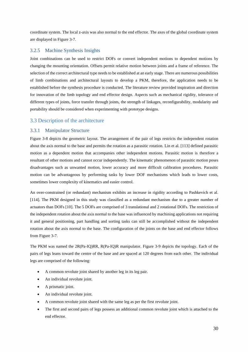
30
coordinate system. The local z-axis was also normal to the end effector. The axes of the global coordinate system
are displayed in Figure 3-7.
3.2.5 Machine Synthesis Insights
Joint combinations can be used to restrict DOFs or convert independent motions to dependent motions by
changing the mounting orientation. Offsets permit relative motion between joints and a frame of reference. The
selection of the correct architectural type needs to be established at an early stage. There are numerous possibilities
of limb combinations and architectural layouts to develop a PKM, therefore, the application needs to be
established before the synthesis procedure is conducted. The literature review provided inspiration and direction
for innovation of the limb topology and end effector design. Aspects such as mechanical rigidity, tolerance of
different types of joints, force transfer through joints, the strength of linkages, reconfigurability, modularity and
portability should be considered when experimenting with prototype designs.
3.3 Description of the architecture
3.3.1 Manipulator Structure
Figure 3-8 depicts the geometric layout. The arrangement of the pair of legs restricts the independent rotation
about the axis normal to the base and permits the rotation as a parasitic rotation. Lin et al. [113] defined parasitic
motion as a dependent motion that accompanies other independent motions. Parasitic motion is therefore a
resultant of other motions and cannot occur independently. The kinematic phenomenon of parasitic motion poses
disadvantages such as unwanted motion, lower accuracy and more difficult calibration procedures. Parasitic
motion can be advantageous by performing tasks by lower DOF mechanisms which leads to lower costs,
sometimes lower complexity of kinematics and easier control.
An over-constrained (or redundant) mechanism exhibits an increase in rigidity according to Pashkevich et al.
[114]. The PKM designed in this study was classified as a redundant mechanism due to a greater number of
actuators than DOFs [10]. The 5 DOFs are comprised of 3 translational and 2 rotational DOFs. The restriction of
the independent rotation about the axis normal to the base was influenced by machining applications not requiring
it and general positioning, part handling and sorting tasks can still be accomplished without the independent
rotation about the axis normal to the base. The configuration of the joints on the base and end effector follows
from Figure 3-7.
The PKM was named the 2R(Pa-IQ)RR, R(Pa-IQ)R manipulator. Figure 3-9 depicts the topology. Each of the
pairs of legs leans toward the centre of the base and are spaced at 120 degrees from each other. The individual
legs are comprised of the following:
• A common revolute joint shared by another leg in its leg pair.
• An individual revolute joint.
• A prismatic joint.
• An individual revolute joint.
• A common revolute joint shared with the same leg as per the first revolute joint.
• The first and second pairs of legs possess an additional common revolute joint which is attached to the
end effector.

31
Figure 3-8: Geometric layout of the PKM
Figure 3-9: Machine Topology

32
3.3.2 Machine Novelties and Characteristics
The 2R(Pa-IQ)RR, R(Pa-IQ)R possessed the following novelties and characteristics:
• All prismatic joints are actuated and all potential universal joints have been decoupled into revolute
joints.
• The position and orientation of the pairs of legs collectively restricts the independent rotation about the
axis normal to the base (z-axis) and permits the rotation as a parasitic rotation.
• When the end effector exhibits translation, then the pairs of legs maintain a parallelogram structure as
each pair is actuated by equal stroke lengths. Each pair of legs could be actuated by a different stroke
length to another pair.
• The arrangement of the revolute joints constrains each of the legs within a pair to be coplanar.
• The rotation was achieved when the legs within a pair are actuated to different lengths. The
parallelogram structure changes into an irregular quadrilateral.
The DOF of a PKM is generally calculated by using the Grubler or Kutzbach criterion and is presented below [9]:
𝐹 = 𝜆(𝑛 − 𝑗 − 1) + ∑𝑓𝑖
𝑖
(3.1)
Where 𝜆 = 6 for spatial manipulators, 𝑛 is the number of links of the mechanism, 𝑗 is the number of joints with
the assumption that all joints are binary and 𝑓𝑖 is the relative motion allowed by joint 𝑖. For the PKM developed
in through this study the aforementioned parameters are as follows:
• 𝜆 = 6 as this is a spatial manipulator.
• 𝑛 = 28 as this is the total number of links.
• 𝑗 = 32 as the manipulator possesses 20 binary joints and 6 ternary joints which (counts as 2 binary joints
each). Therefore, the total number of joints is the sum of these two values.
• 𝑓𝑖 = 𝑓1 = 26 as there are 6 prismatic joints and 20 revolute joints and each of these joints permits one
DOF thus, the total number of one DOF joints is 26.
The DOFs can be calculated using the Grubler/Kutzbach equation.
𝐹 = 6(28 − 32 − 1) + 26 = −4 (3.2)
A robotic manipulator cannot possess a negative number of DOFs. The negative value is interpreted as the PKM
being an over-constrained mechanism, as stated by Merlet [10]. Over-constrained mechanisms can potentially
increase rigidity. These mechanisms constrain the end effector to prevent one or more translations or rotations.
The over-constrained nature includes more complicated kinematic and stiffness modelling [114]. It was previously
stated that the PKM possessed 5 DOFs and a parasitic rotation. This was identified through observations and
measurements conducted in SolidWorks® due to the breakdown of the Grubler/Kutzbach equation for over-
constrained mechanisms. Appendix G illustrates the different DOFs exhibited by the PKM confirming its 5 DOFs
with a parasitic rotation.

33
Lin et al. [113] suggested that parallel mechanisms exhibiting parasitic motion should be classified according to
type of parasitic motion, scale and motion pattern. The PKM developed was classified as follows:
• Type: The PKM possessed a rotational parasitic motion induced by 2 independent rotations of the end
effector hence the parasitic motion characteristic is symbolised as 𝑅⨁{𝑅}. The term within the brackets,
represents the dependent motion and in this instance the symbol 𝑅 refers to rotation.
• Scale: The scale refers to the amplitudes of the independent and dependent motions relative to each other.
In terms of scale, the PKM was classified as Finite-Finite since the dependent motion can sometimes be
greater than one of the independent rotations that cause its occurrence and all motions were finite. The
parasitic motion was not infinitesimal and was therefore not classified as Finite-Infinitesimal. The
parasitic motion was not always smaller than both independent rotations and therefore could not be
classified as Finite-Small.
• Motion pattern: The motion pattern summarises the representation of motions. The PKM possess 3 and
2 independent translations and rotations respectively and is represented as 3𝑇2𝑅. Considering the
parasitic motion, the motion pattern of the PKM is then represented as 3𝑇2𝑅⨁{𝑅}. Due to one parasitic
motion incurred, the dimension of parasitic motion is 1.
The PKM possessed similarities to the Hexapod (Stewart-Gough Platform) in appearance [8]. Differences between
the 2R(Pa-IQ)RR, R(Pa-IQ)R PKM and the Hexapod are listed in Table 3-2.
Table 3-2: Differences between the novel architecture and the Hexapod
Architecture 2R(Pa-IQ)RR, R(Pa-IQ)R Hexapod
DOF 5 6
Joints Prismatic and revolute Various combinations of prismatic,
revolute, spherical and universal joints
Pairs of legs Yes No
Common joints Yes Sometimes
Attachment points to base 3 6
Attachment points to end effector 4 6
Some actuators move completely
in space
Yes No
3.4 Quality Function Deployment
The QFD analysis is performed to assist in generating target specifications. The QFD analysis relates the
customers’ requirements into engineering metrics. Engineering metrics can, therefore, clash with each other and
reasonable trade-offs are required. The QFD analysis also helps the designer to benchmark the product against its
competitors thus establishing the product’s advantages and disadvantages. Obtaining target specifications is a
priority of performing the QFD analysis. The aim is to produce a product that results in customer satisfaction
however, the difficulty to change different engineering metrics is not equal. The QFD analysis reveals which
engineering metrics are critical to the designer/engineer[115]. This research used the House of Quality QFD
template. Appendix D presents the QFD.

34
3.4.1 Relationship between Customer Requirements and Engineering Metrics
Each customer requirement has at least one strong relationship with an engineering metric. The rotation about the
x and y axes had the highest number of strong relationships with engineering metrics. This indicated that the
rotational capability of the machine is the most sensitive customer requirement for changes in engineering
parameters. Most customer requirements have approximately 4 strong relationships with engineering metrics. The
durable and lightweight customer requirements have only 2 strong relationships with engineering metrics and are,
therefore the least affected by changes in engineering metrics. The stroke length of the linear actuators possessed
the highest number of strong relationships with customer requirements. This engineering metric is, therefore, one
of the most important metrics to consider.
There are also moderate and weak relationships that exist between customer requirements and engineering
metrics. An example of a medium relationship exists between the customer requirement of a modular PKM and
the mass of the motors. If the motors are heavy, it makes modularity challenging in terms of reconfiguration,
assembly and decommissioning. A weak relationship was observed between the PKM being portable and the
volume of the end effector. The volume of the end effector, therefore, its mass, influences the portability of the
robotic platform but the relationship does not bear strong nor moderate influences to be of significant concern.
3.4.2 Relationship between Engineering Metrics
Engineering metrics can either be supportive or conflicting. An example of a strong positive (supportive)
relationship is the relationship between the range of motion along the x-axis the stroke length of the linear
actuators. The stroke length of the actuator significantly affects the range of motion along the x-axis. When the
stroke length of the linear actuator is increased, the range of motion in the x-direction is increased. These
parameters are intended to be increased and therefore, they have a strong positive correlation. A positive
correlation was observed between the mass of the motors and the mass of the actuators. These parameters are
aimed to be minimised to create a lightweight PKM. When the mass of the motors is decreased, the mass of the
linear actuators is decreased and is, therefore, a supportive relationship.
A conflicting relationship was discovered between the range of motion along the x-axis and number of
singularities. The range of motion is aimed to be increased but an increase in range of motion allows the possibility
of more singularities to occur within the workspace of the robot. The number of singularities was aimed to be a
minimum. This was noted as a negative correlation. A strong negative relationship was discovered between the
stroke length of the actuators and the number of singularities. The stroke length should be as large as possible but
also increases the likelihood of the number of singularity points that can exist. The rest of the engineering metrics
were assessed in the same way as presented.
3.4.3 Importance Ratings, Relative Weight and Difficulty of Target
The importance rating considers the relationship strength between the various customer requirements and
engineering metrics. The relative weight value highlights the significance of each engineering metric relative to
each other. For example, the stroke length of the linear actuator was ranked with the highest importance due to its
strong relationship with many customer requirements. The second-highest ranked engineering parameters were
accuracy and repeatability. These parameters require more design and investigation than others that ranked lower.
For example, accuracy should require more design and investigation than the mass of the linear actuators.

35
The difficulty in reaching the target specification was vital because it also influenced how much time should be
spent to optimise a parameter and highlighted how dependant a parameter is on others. For example, the target
value for the motor of an actuator is 2 kg and rated with a difficulty of 2/10. The mass can be easily achieved
through purchasing off-the-shelf motors and is not dependent on other factors. However, the accuracy is rated as
8/10. The difficulty is due to the high dependence on other components and cannot be easily achieved as the mass
of the motor. This understanding was carried forward into the detailed mechanical design.
3.4.4 Target Specifications
One of the aims of the QFD analysis was to develop target specifications. Table 3-3 presents the engineering
metrics, target specifications and justifications. The target specifications influenced the design of the components
presented in Section 4.
Table 3-3: Target Specifications
Engineering Metric Target
Specification
Justification
Mass of motors (Total) 2 kg 6 x NEMA 17 motors should not exceed a mass of 2
kg. NEMA 17 motors are chosen for a compact
prototype.
Mass of linear actuators (Total) 4kg The prototype is aimed to be lightweight.
Range of motion in the x-direction 200 mm Reasonable estimations were made since this is
dependent on the stroke length of the linear actuators. Range of motion in the y-direction 250 mm
Range of motion in the z-direction 100 mm
Minimum degrees of tilt about X
and Y-Axis
At least 60° Most commercially available 5-DOF and 6-DOF
PKMs have a range of 50°.
Stroke length of linear actuators 65 mm A reasonable estimation for a compact prototype.
Area of base 1 m2 The base should easily account for changes made to
the mounting pattern if required.
Volume of end effector 0.00004 m3 A reasonable estimation for a compact prototype.
Spacing between actuators 90 mm There would be enough clearance to avoid self-
clashing of the actuator legs whilst not designing
mounting brackets to be too large.
Volume of footprint (compactness) 0.003 m3 A compact prototype was aimed to be developed as
proof of concept. This was estimated to be a
tetrahedron when the PKM is fully retracted.
Singularities in workspace volume 0 Ideal case for any robotic platform.
Tolerance of joints ≤1 mm To aim for high accuracy and repeatability.
Accuracy 2 mm and 2° A desktop prototype developed through AM was used
for experimentation without the use of high accuracy
components.
Repeatability 2 mm and 2°
36
3.4.5 Competitive Analysis
A competitive analysis was conducted between industrial PKMs and the PKM developed in this researched. The
PKM developed was the most favourable concerning weight, cost, modularity and portability. These criteria
possessed a strong relationship to each other. The PKM was specified to be developed through AM. This allowed
the PKM to be lightweight, be considerably cheaper and more portable than industrial PKMs. The modularity
criterion was ranked favourably due to the ease at which the machine can be reconfigured aided by AM.
The PKM was the least favourable concerning translation along the x, y and z axes, durability, high precision and
use for different applications. The PKM was aimed to be developed as a desktop prototype hence, considerably
smaller than industrial PKMs. The size of the PKM is influenced by the stroke length of the linear actuators. A
target specification aimed to produce actuators that possessed a 65 mm stroke length therefore the translation
along the x, y and z axes were the least favourable in comparison to industrial PKMs. The PKM was the least
durable due to AM. AM permits larger joint tolerances than industrial joints therefore tasks prone to vibrations
would cause the PKM to be the least durable. Moreover, the PKM would be the least durable under heavy loads
as opposed to industrial PKMs. The larger joint tolerances would pose a challenge in obtaining high accuracy and
repeatability.
The PKM’s use in different applications was ranked the lowest due to the limitations induced through AM. All
PKMs in the competitive analysis were capable of being employed for multiple functions and the PKM developed
could also be used in this manner should a large-scale prototype be developed. The target specification of at least
60° of rotation about the x and y axes was favourable since only the Metrom Pentapod P800 possessed larger
ranges of tilt. Other PKMs ranges of tilt generally did not exceed ±25°. The FANUC F-200iB and the Hexapode
300 were ranked the best concerning its use for different applications which is strongly influenced by the
portability criterion.
The Metrom Pentapod P800 and the FANUC F-200iB were the best PKMs for benchmarking. The Metrom
Pentapod P800 ranked the best on three instances and ranked the least favourable only once. The FANUC F-200iB
was the least favourable and most favourable only once. It was consistently competitive against industrial PKMs.
The Metrom Pentapod P800 and the FANUC F-200iB can both be used for drilling and milling operations however
the FANUC F-200iB is generally mounted in different orientations since it is more portable. The PKM in this
study aimed to improve the rotational capabilities of industrial PKMs as well as being relatively lightweight.
Larger PKMs such as the OKUMA PM600 and the Metrom Pentapod P800 generally possess higher accuracy
and repeatability than other PKMs but possess drawbacks of poor portability, high costs and are extremely heavy.
The PKM in this study possessed extreme characteristics by ranking the best and least favourable in 4 instances
each. This was strongly influenced by the production through AM. The QFD competitive analysis was not a true
reflection of machine performance as it compared customer requirements and not engineering ratios such as
actuator stroke length to translation along the x, y and z axes and others. The size of the robotic platform
determined many machine characteristics hence, performance and engineering ratios are better suited as a method
of comparison.

37
3.5 Chapter Summary
This chapter discussed the PKM synthesis procedure and presented the sequential formulation of the architectural
design. The structure and the PKM novelties were presented and the robotic platform was classified as an over-
constrained mechanism. The PKM possessed 5 DOFs and a parasitic rotation. The QFD analysis was presented
which aided in generating target specifications. Potential customer requirements and their relationships to
engineering metrics were reviewed. The relationships between the various engineering metrics were analysed. A
competitive analysis was conducted between industrial PKMs and the PKM developed in the study.
The next chapter presents the mechanical design of the PKM. A design methodology and a system decomposition
diagram are presented. The prototype was designed for AM and the design considerations are discussed. The
various components designed are presented. The PKM specifications, sub-assembly and assembly precedence
diagrams are presented.

38
4. MECHANICAL DESIGN
The mechanical design methodology is described. A detailed mechanical design was performed using the target
specifications obtained from the QFD analysis. Component designs are presented with consideration for AM. A
low-cost desktop prototype was designed and built to demonstrate the motion characteristics of the PKM. The
final specifications are presented. Sub-assembly and assembly precedence diagrams are presented.
4.1 Mechanical Design Methodology
The mechanical design process is illustrated in Figure 4-1. Shaik [37] presented and followed this process to
develop a sensor system for a pick and place PKM. The method was also described by Merlet [116]. The structural
and dimensional syntheses were performed concurrently. The machine topology, regarding the PKM type, was
addressed in Section 3. Concerning, the actuators, the position of the foot points of the legs relative to each other
was 120° as per Figure 3-7. The PCD of the footpoints, the actuator stroke length and mounting distance between
actuators in a leg pair were iteratively designed through 3D CAD modelling.
Components were iteratively designed on SolidWorks® due to designing for workspace preferences concurrently.
SolidWorks® allowed the joints and assembly to move and measurements were taken, shown in Figure 5-3.
Dimensional synthesis concerning workspace and singularities was addressed iteratively. Final engineering
drawings are presented in Appendix H. Workspace was dependent on the range of motion along the x, y and z
axes. The range of motion was mainly dependant on actuator stroke length, PCD of the footpoints, mounting
distance between actuators in a leg pair and end effector design. The PKM was designed to be compact and with
sufficient strength for demonstration. A high range of motion along the x and y axes was preferred to define the
workspace. Workspace is the most significant factor that influences geometric parametrisation of the PKM as per
Figure 4-1.
Figure 4-1: Mechanical design process for a PKM [37]

39
4.2 System Decomposition Diagram
Figure 4-2 illustrates the system decomposition diagram.
Figure 4-2: Mechanical system decomposition diagram
4.3 Design for Additive Manufacturing
AM machines possess parameters such as infill density, layer height, infill pattern and type of scaffolding that
alter the print quality. These factors were taken into account. All drawings for the components are presented in
Appendix H.
4.3.1 Material Selection
Table 4-1 compares the properties of Acrylonitrile Butadiene Styrene (ABS) and Polylactic Acid (PLA),
according eSun [117]. PLA filament was selected as the material for production due mainly to its lower print and
bed temperature. The lower bed temperature allowed a faster production of components. PLA possesses a higher
tensile strength and bending strength than ABS filament. ABS printed components are more susceptible to
warpage. Appendix E presents the cost of the materials.
PK
M
Linear actuators Stepper motor
Back plate
Outer casing
Flexible coupler Threaded rod
Nut
Telescoping arm
Revolute joints
Thrust bearing joint for legs 1 - 4
Top housing
Bottom housing
Thrust bearing
Radial bearings
Base-mounted for legs 5 and 6
On the end effector
Top and bottom of actuators
End effector Aluminium rod
Base
Mounting brackets
Bottom of actuators
For Leg 1 - 4
For leg 5 and 6 Aluminium rodTop of actuators
for Leg 1 - 4Spacing blocks

40
Table 4-1: Comparison between ABS and PLA
Property ABS PLA
Print temperature (°C) 220-260 190-210
Bed temperature (°C) 110 No Heat/(60-80)
Density (g/cm3) 1.04 1.24
Distortion temperature (°C, 0.45MPa) 78 56
Melt flow index (g/10min) 12 (220 °C/10kg) 5 (190 °C/2.16kg)
Tensile strength (MPa) 43 65
Elongation at break (%) 22 8
Bending strength (MPa) 66 97
Flexural modulus (MPa) 2348 3600
IZOD impact strength (KJ/m2) 19 4
4.3.2 Material Wastage, Manufacturing Time and Clearances
Manufacturing time was considered due to the large number of components designed. A print infill of 80% was
used with a layer height of 0.2 mm. Print orientation was considered to reduce the scaffolding produced while
maximising the strength of the component.
A revolute joint was used as the test piece for testing joint tolerances. The forked end of the revolute joint was
printed with a gap of 8 mm. Various complimenting test pieces with different widths were printed. The tests
revealed that the best clearance for press fits and joints was 0.1 mm and 0.2 mm respectively. When scaffolding
was produced, the press-fit clearance changed from 0.1 mm to 0.3 mm. All components were designed with these
clearances.
4.3.3 Linear Actuator
The linear actuator affects mechanical strength, rigidity, inertia, workspace and cost. Appendix F presents the
various linear actuator concepts and the selection matrix used to select the most suitable concept. The final concept
was a variation of concept 3. The guides from the outer casing and the slots from the telescoping arm from concept
3 were removed due to the cantilever effect at the front of the actuator. This increased accuracy. The disadvantage
was that it required more scaffolding than concept 3, and therefore, light filing was required to smoothen the areas
where scaffolding was developed. The linear actuators had a stroke length of 66 mm. Figure 4-3 depicts an
exploded view of concept 4. Appendix C.1 and C.2 presents the power screw and buckling analysis respectively.
The buckling analysis revealed that the critical load was 16.80 kN. Appendix H presents the technical drawings.
Figure 4-3: Linear actuator concept 4
Telescoping
arm lip
Outer
casing lip

41
4.3.4 Revolute Joints
4.3.5 Revolute joints on end effector and linear actuators
The revolute joints follow a clevis joint design with one end in the form of a fork and the other end a matching
rod end. The revolute joints were designed with sufficient height to avoid self-clashing. Figure 4-4 (a) to (e)
illustrates the forked and rod components of the revolute joints. The gap of forked end of the revolute joints was
8 mm in width and the thickness of each protrusion was 8 mm.
There was a design variation between the revolute joints shown in Figure 4-4 (b) and (c). Actuators 5 and 6 are
positioned side-by-side as opposed to one being vertically above the other. The revolute joints in Figure 4-4 (c)
were designed to be mounted to an aluminium rod.
4.3.6 Thrust bearing revolute joint
The mounting bracket for the bottom of actuators 1-4 was designed to rotate. Figure 4-4 (f) shows an exploded
view the thrust bearing revolute joint. It comprised of 7 components. The radial bearings allowed smooth rotation
of the bolt which locked the entire unit together with the lock nut. The top housing component served as a swivel
plate for the linear actuator mounting bracket. Specifications for the radial bearing and the thrust bearing are
provided by 3D Printing Store and RS components respectively [118, 119]
Figure 4-4: Revolute joints
a. Revolute joint attached to the end effector
b. Revolute joint attached to the top and bottom of actuator 5 and 6
c. Revolute joint attached to the top and bottom of actuator 1-4
d. Revolute joint attached to the telescoping arm
e. Revolute joint attached to the back of the stepper motor
f. Exploded view of the revolute joint attached to the mounting bracket for the bottom of actuators 1-4
a. b.
c.
d. e.
f.

42
4.3.7 End Effector and Base
4.3.7.1 End effector and related revolute joints
The end effector was designed to be triangular with revolute joints at each of its corners to accommodate for the
three pairs of legs. One corner of the end effector was designed to possess revolute joint oriented horizontally to
accommodate the third pair of legs which were side-by-side. An aluminium rod rotated within the horizontal hole.
The end effector designed was based on an equilateral triangle and possessed a thickness of 8 mm. Figure 4-5
displays the end effector.
Figure 4-5: The end effector
4.3.7.2 Base and spacing of mounting points
The distance from the center of the base to the leg mounting points and the angular spacing between them are
factors that influence workspace, singularities, stiffness, etc. A leg spacing of 120° relative to each other and
distance of 150 mm from the base center was chosen. Depending on the intended workspace, the mounting points
on the base can be altered.
4.3.8 Mounting Brackets and Spacing Blocks
4.3.8.1 Mounting bracket for the bottom of actuators 1-4
The bottom bracket for the bottom of actuators 1-4 was designed with mounting points at for each actuator in the
leg pair. Two brackets were implemented for the first and second pairs of legs. This bracket is connected to the
thrust bearing revolute joint.
This bracket was designed with a reinforcing gusset to restrict bending. There can be various mounting points
designed into the vertical length of the bracket to allow for reconfigurability. The height of the bracket could also
be extended to increase the distance between mounting points. The mounting bracket for the bottom of actuators
1-4 is shown in Figure 4-6 (a).
4.3.8.2 Mounting bracket for the top of actuators 1-4
The mounting bracket for the top of actuators 1-4, illustrated in Figure 4-6 (b), was designed to mirror the vertical
face of the bottom mounting bracket with the same layout for the attachment points of the revolute joints. This
ensured the pair of legs remain parallel when the end effector exhibits translational motion. The revolute joint
shown in Figure 4-4 (a) connects the mounting bracket for the top of actuators 1-4 to the end effector.
Revolute
joints

43
4.3.8.3 Mounting bracket for the bottom of actuator 5 and 6
The mounting bracket for the bottom of actuator 5 and 6 was designed with a common revolute joint shared by
actuator 5 and 6. The bracket possessed a supporting gusset on either side to increase rigidity. An aluminium rod
passed through the top of the bracket and could freely rotate. The revolute joints at the bottom of linear actuator
5 and 6 were bolted onto the aluminium rod. The bracket is depicted in Figure 4-6 (c).
4.3.9 Spacing Blocks
The spacing blocks were designed to assist in the prevention of self-clashing of the legs within the same pair. The
spacing blocks were designed to suit the length and width of the mounting brackets at the top and bottom of the
linear actuators. The height of the spacing blocks was chosen to be 20 mm as it suffices to prevent self-clashing
of the legs in the rest position. The height of the spacing blocks can be designed to suit the angle at which the legs
lean forward to prevent self-clashing if other machine parameters are changed. Figure 4-6 (d) illustrates the
spacing block.
Figure 4-6: Mounting brackets and spacing block
a. Mounting bracket for the bottom of actuators 1-4
b. Mounting bracket for the top of actuators 1-4
c. Mounting bracket for the bottom of actuator 5 and 6
d. Spacing block
4.4 PKM Specifications
Once the PKM components were design and assembled in SolidWorks®, the machine specifications could be
determined. All parameters were reasonably close to the target specifications from the QFD analysis except for
the area of the base. This was reduced by 60%. Table 4-2 presents the PKM specifications.
a. b. c.
d.

44
Table 4-2: PKM specifications
Aspect Specification
Mass of linear actuators (Total) 3.5 kg
Range of motion in the x-direction 188.64 mm
Range of motion in the y-direction 272.24 mm
Range of motion in the z-direction 94.6 mm
Degrees of tilt about the x-axis 71.46°
Degrees of tilt about the y-axis 63.97°
Stroke length of linear actuators 66 mm
Area of base 0.4 m2
Volume of end effector 0.00035 m3
Spacing between actuators 80 mm
Tolerance of joints ≤1 mm
4.5 Sub-assembly Precedence Diagrams
The sub-assembly precedence diagrams are presented. Figure 4-7 shows the thrust bearing sub-assembly diagram
and Table 4-3 presents the components descriptions and quantities. There are 2 identical thrust bearing assemblies
and Figure 4-7 describes the sub-assembly for 1 unit.
Figure 4-7: Thrust bearing sub-assembly diagram
Table 4-3: Thrust bearing sub-assembly description and bill of materials
Item Description Quantity Item Description Quantity
1 Bottom housing 1 5 Bottom race 1
2 Top housing 1 6 Top race 1
3 Bottom radial bearing 1 7 Inner race 1
4 Top radial bearing 1 8 Bolt and lock nut 1
Figure 4-8 shows the linear actuator sub-assembly diagram for one actuator. There are 6 actuators used in the
design. Table 4-4 displays the corresponding descriptions and quantities.
Figure 4-8: Linear Actuator sub-assembly diagram
1 2 3 4 5 6
1
2
3
4
5
6
7 8

45
Table 4-4: Linear actuator sub-assembly description and bill of materials
Item Description Quantity Item Description Quantity
1 Joint B part 2 1 4 Threaded rod 1
2 Stepper motor 1 5 Telescoping arm 1
3 Flexible coupling 1 6 Actuator casing 1
The assembly of the PKM is described by Figure 4-9. The subassembly of path 2 is applicable to leg pair 1 and 2
and leg pair 3 and 4 since they are identical. Table 4-5 describes the components used and the quantities.
Figure 4-9: PKM sub-assembly diagram
Table 4-5: PKM sub-assembly description and bill of materials
Item Description Quantity Item Description Quantity
1 Wooden base 1 11 Actuator sub-assembly 4
2 Thrust bearing sub-
assembly
2 12 Revolute joints 2
3 Joint B bracket variation
2
1 13 Spacer block 2
4 Leg 1/3 and 2/4 Joint B
bracket variation 1
2
14 Revolute joint 2
5 Aluminium rod 1 15 Aluminium rod 1
6 Revolute joint 2 16 Revolute joint 2
7 Spacer block 2 17 End effector mounting
bracket
2
8 Revolute joints 2 18 Revolute joint 2
9 Revolute joint 2 19 End effector 1
10 Actuator sub-assembly 2
4 2
1
7
10 12 5 8
11
13
14
6
9
3 15
16
19
17 18

46
XY optical mouse sensor sub-assembly diagram is shown by Figure 4-10 and the component description and
quantities are listed in Table 4-6.
Figure 4-10: XY mouse sub-assembly diagram
Table 4-6: XY mouse optical sensor sub-assembly description and bill of materials
Item Description Quantity Item Description Quantity
1 End effector 1 3 XY optical mouse 1
2 XY mouse bracket 2 1 4 XY mouse bracket 1 1
The testing frame developed for this research was set up differently to accommodate testing for translation and
rotation. Figure 4-11 shows the testing frame sub-assembly diagram for translation testing. Table 4-7 describes
the various components and quantities.
Figure 4-11: Testing frame for translation sub-assembly diagram
Table 4-7: Testing frame for translation sub-assembly description and bill of materials
Item Description Quantity Item Description Quantity
1 Aluminium profiles 12 8 Linear bearings 4
2 XY mouse sensor sub-
assembly
1 9 Mouse bracket 2 1
3 Z optical mouse 1 10 Mirror bracket 1 2
4 90° connectors 20 11 Chromed linear shaft 4
5 Wooden platform 1 12 Mirror 1
6 Mouse Z bracket 1 1 13 Bottom shaft supports 4
7 Mirror bracket 2 2 14 Top shaft supports 4
1 2 3 4
4 1
2
3
7 10 12
6
5 8 11
9
13 14

47
The testing frame for rotation testing is shown in Figure 4-12. An additional level comprised of aluminium
extruded profiles were required. Table 4-8 shows the components used and quantities.
Figure 4-12: Testing frame for rotation sub-assembly diagram
Table 4-8: Testing frame for rotation sub-assembly description and bill of materials
Item Description Quantity Item Description Quantity
1 Aluminium extruded
profiles basic frame
12 5 Mirror bracket 1
2 Aluminium extruded
profiles additional level
7 6 Vernier calliper brackets 2
3 End effector 1 7 Mirror 1
4 90° connectors 50 8 Vernier calliper 1
4.6 Assembly Precedence Diagram
Figure 4-13 shows the assembly diagram. Table 4-9 provides the descriptions and quantities of the components
shown in Figure 4-13.
Figure 4-13: Project assembly diagram
Table 4-9: Project assembly description and bill of materials
Item Description Quantity Item Description Quantity
1 Wooden base 1 5 Control Box 1
2 PKM sub-assembly 1 6 Testing frame sub-
assembly
1
3 Wood inserts 16 7 PC 1
4 Aluminium 90° supports 8
2 5
3 4 6
7 1
1
5
2
4
7
8
6
3

48
4.7 Chapter Summary This chapter presented the mechanical design methodology and the system decomposition diagram. This chapter
also described the mechanical design of the various components while considering AM parameters. The PKM
specifications were documented. The sub-assembly and assembly precedence diagrams were presented. The
following chapter discusses kinematic analysis. The inverse kinematic analysis is first presented which discusses
the selected method of analysis and the homogenous transformation matrix. A novel extension of the geometric
method is presented. The top layer of Simulink model for the inverse kinematics is presented with a tabulation of
the various functions used to develop the model. The forward kinematic analysis is presented. The Newton
Raphson (NR) method was employed and the constraint equations are presented.

49
5. KINEMATIC ANALYSIS
5.1 Introduction
The inverse kinematic analysis solves the actuator lengths or joint angles for a specified position and orientation
of the end effector. The forward kinematic analysis solves the position and orientation of the end effector for a
given set of actuator lengths or joint angles. The two commonly used methods for position and orientation analysis
are the Denavit-Hartenberg (DH) method and the geometric method. The geometric method generates a vector
loop to solve the position and orientation of the end effector. The DH method can be easily used for serial
manipulators but is complicated for multiple closed-loop kinematic chains. Tsai [9] presented numerous examples
of the geometric method and it was concluded as a feasible approach.
5.2 Homogenous Transformation Matrix
Concerning robotics, multiple coordinate systems are employed to assist in the computations of a robot’s
parameters such as inverse and forward kinematics, velocities and accelerations. The placement and number of
coordinate systems used are up to the designer. However, the positions and orientations need to be homogeneously
mapped from one coordinate system to another using a homogenous transformation matrix. This matrix is divided
into four submatrices and is shown in Equation 5.1 [9]:
𝑇𝐵𝐴 = [
𝑅𝐵𝐴 (3𝑥3) ⋮ 𝑞𝐴 (3𝑥1)
⋯ ⋮ …𝜍 (1𝑥3) ⋮ 𝜌 (1𝑥1)
]
(5.1)
The upper left submatrix holds the orientation matrix of the moving frame B with respect to frame A (the fixed
frame). The upper right submatrix describes the position of the origin of the moving frame 𝐵 with respect to frame
𝐴 and is a position vector. The lower left submatrix denotes at perspective transformation and the lower right
submatrix represents a scaling factor. The study of robotic manipulators and kinematics of mechanisms sets the
scaling factor to 1 and the perspective transformation to zero. The matrix is presented in Equation 5.2 [9]:
𝑇𝐵
𝐴 = [𝑅𝐵
𝐴 (3𝑥3) ⋮ 𝑞𝐴 (3𝑥1)⋯ ⋮ …
0 0 0 ⋮ 1
]
(5.2)
5.3 Inverse Kinematics
The methodology that was employed to generate, solve and validate the inverse kinematic equations is listed
below:
1. Establish a rotation sequence.
2. Perform the outer vector loop analysis.
3. Perform the inner vector loop analyses.
4. Develop a MATLAB® script to solve the inverse kinematic equations.
5. Validate the equations via SolidWorks®.
6. Develop the Simulink model.
7. Validate the Simulink model via SolidWorks.

50
The Roll, Pitch and Yaw rotation sequence was used. The order of rotations is not commutative therefore, a
rotation sequence needed to be established [9]. The order of rotation takes place about the x-axis (Roll), then the
y-axis (Pitch) and finally the z-axis (Yaw). The rotation matrix is given by Equation 5.3.
𝑅(𝛾, 𝛽, 𝛼) = [
𝑐𝛾 𝑐𝛽 𝑐𝛾 𝑠𝛽 𝑠𝛼 − 𝑠𝛾 𝑐𝛼 𝑐𝛾 𝑠𝛽 𝑐𝛼 + 𝑠𝛾 𝑠𝛼𝑠𝛾 𝑐𝛽 𝑠𝛾 𝑠𝛽 𝑠𝛼 + 𝑐𝛾 𝑐𝛼 𝑠𝛾 𝑠𝛽 𝑐𝛼 − 𝑐𝛾 𝑠𝛼−𝑠𝛽 𝑐𝛽 𝑠𝛼 𝑐𝛽 𝑐𝛼
]
(5.3)
Where 𝑐 = 𝑐𝑜𝑠𝑖𝑛𝑒 𝑎𝑛𝑑 𝑠 = 𝑠𝑖𝑛𝑒
The case of parasitic motion was not investigated in this study therefore the rotation about the z-axis was regarded
as 𝛾 = 0. For 𝛾 = 0, the simplified rotation matrix is shown in Equation 5.4.
𝑅(𝛽, 𝛼) = [𝑐𝛽 𝑠𝛽 𝑠𝛼 𝑠𝛽 𝑐𝛼0 𝑐𝛼 −𝑠𝛼
−𝑠𝛽 𝑐𝛽 𝑠𝛼 𝑐𝛽 𝑐𝛼]
(5.4)
5.3.1 Extension of the Geometric Method
The geometric method applied to solve the inverse kinematics is a novel extension due to the existence of offset
revolute joints. The offsets introduce passive angles, therefore, more variables [111, 120]. The architectural design
was exploited. Outer and inner vector loops were employed. Figure 5-1a shows a side view of the PKM and a
vector loop generally employed. The general vector loop uses four points of interest to construct the vector loop.
The vector over-arching the linear actuator is meant to be the only unknown variable (vector). The vector of
interest, as shown in Figure 5-1, is identified in red. The red vector, representing the vector from the base to the
bottom of the actuator, changes as the end effector moves is, therefore, a free variable as depicted in Figure 5-1b
and Figure 5-1c. The position of the bottom of the linear actuator moves along an arc, represented in orange, as
the PKM moves.
Figure 5-1: General vector diagram with the top view of the PKM
a. The red arrow highlighting the vector from 𝑂 to 𝐵.
b. The end effector in its home position.
c. The change in the length and direction of the red vector.
a. b. c.

51
5.3.2 Inverse Kinematic Relationships through the Outer Vector Loop Method
Figure 5-2 depicts the outer vector loop for actuators 1 and 2. The outer vector loop was developed such that the
passive rotations occurring at points 𝐴, 𝐵, 𝐶 and 𝐷 do not need to be known in order to perform the inverse
kinematic analysis. Two different paths are taken from point 𝑂 to point 𝐷.
The vectors used in Equation 5.5 were chosen such that 𝑂𝐴 and 𝑃𝐷 are machine parameters. Point 𝑃 is a user-
defined input of the position of the end effector. It follows that vector 𝑂𝑃 is a user-defined vector. The only
unknown is the vector 𝐴𝐷 . The coordinates of vector 𝑃𝐷 are known relative to a local coordinate frame placed at
point 𝑃. Vector 𝑃𝐷 rotates and a rotational matrix was multiplied to it to resolve its position relative to the global
coordinate frame placed at point 𝑂. The resulting equation can be applied to the leg pair 3 and 4 as well as for
leg pair 5 and 6. The generic outer vector loop equation is given by Equation 5.5
𝑂𝐴 + 𝐴𝐷 = 𝑂𝑃 + 𝑅(𝛾, 𝛽, 𝛼)𝑃𝐷 (5.5)
Figure 5-2: Outer vector loop
Equation 5.6 describes the outer vector shown in Figure 5-2. Equation 5.6 is expanded to Equation 5.7 and 5.8 to
illustrate the methodology of performing the outer vector loop analysis.
𝑂𝐴1,2 + 𝐴1,2𝐷1,2
= 𝑂𝑃 + 𝑅(𝛽, 𝛼)𝑃𝐷1,2 (5.6)
[ (𝑂𝐴1,2
)𝑥
(𝑂𝐴1,2 )
𝑦
(𝑂𝐴1,2 )
𝑧]
+
[ (𝐴1,2𝐷1,2
)𝑥
(𝐴1,2𝐷1,2 )
𝑦
(𝐴1,2𝐷1,2 )
𝑧]
=
[ (𝑂𝑃 )
𝑥
(𝑂𝑃 )𝑦
(𝑂𝑃 )𝑧]
+ [𝑐𝛽 𝑠𝛽 𝑠𝛼 𝑠𝛽 𝑐𝛼0 𝑐𝛼 −𝑠𝛼
−𝑠𝛽 𝑐𝛽 𝑠𝛼 𝑐𝛽 𝑐𝛼]
[ (𝑃𝐷1,2
)𝑥
(𝑃𝐷1,2 )
𝑦
(𝑃𝐷1,2 )
𝑧]
(5.7)
[ (𝐴1,2𝐷1,2
)𝑥
(𝐴1,2𝐷1,2 )
𝑦
(𝐴1,2𝐷1,2 )
𝑧]
=
[ (𝑂𝑃 )
𝑥+ 𝑐𝛽(𝑃𝐷1,2
)𝑥+ 𝑠𝛽 𝑠𝛼(𝑃𝐷1,2
)𝑦
+ 𝑠𝛽 𝑐𝛼(𝑃𝐷1,2 )
𝑧− (𝑂𝐴1,2
)𝑥
(𝑂𝑃 )𝑦
+ 𝑐𝛼(𝑃𝐷1,2 )
𝑦− 𝑠𝛼(𝑃𝐷1,2
)𝑧− (𝑂𝐴1,2
)𝑦
(𝑂𝑃 )𝑧− 𝑠𝛽(𝑃𝐷1,2
)𝑥+ 𝑐𝛽 𝑠𝛼(𝑃𝐷1,2
)𝑦
+ 𝑐𝛽 𝑐𝛼(𝑃𝐷1,2 )
𝑧− (𝑂𝐴1,2
)𝑧 ]
(5.8)

52
Let each equation be isolated as for simplicity as presented by Equation 5.9 to 5.11.
𝐿 = (𝑂𝑃 )𝑥+ 𝑐𝛽(𝑃𝐷1,2
)𝑥+ 𝑠𝛽 𝑠𝛼(𝑃𝐷1,2
)𝑦
+ 𝑠𝛽 𝑐𝛼(𝑃𝐷1,2 )
𝑧− (𝑂𝐴1,2
)𝑥 (5.9)
𝑀 = (𝑂𝑃 )𝑦
+ 𝑐𝛼(𝑃𝐷1,2 )
𝑦− 𝑠𝛼(𝑃𝐷1,2
)𝑧− (𝑂𝐴1,2
)𝑦 (5.10)
𝑁 = (𝑂𝑃 )𝑧− 𝑠𝛽(𝑃𝐷1,2
)𝑥+ 𝑐𝛽 𝑠𝛼(𝑃𝐷1,2
)𝑦
+ 𝑐𝛽 𝑐𝛼(𝑃𝐷1,2 )
𝑧− (𝑂𝐴1,2
)𝑧 (5.11)
The magnitude of vector 𝐴1,2𝐷1,2 is found by the calculation performed in Equation 5.12.
|𝐴1,2𝐷1,2 | = ||
(𝐴1,2𝐷1,2 )
𝑥
(𝐴1,2𝐷1,2 )
𝑦
(𝐴1,2𝐷1,2 )
𝑧
|| = √(𝐿)2 + (𝑀)2 + (𝑁)2
(5.12)
|𝐴1,2𝐷1,2 | was carried forward into the inner vector loop analysis to solve the length of actuator 1.
5.3.3 Inverse Kinematic Relationships through the Inner Vector Loop Method
The inner vector loop equations were reduced to a Two-Dimensional (2D) analysis. Figure 5-3 shows a plane that
actuators 1 and 2 lie along and illustrates the coplanar nature of the pair of legs. Figure 5-3a and Figure 5-3b
shows different views of the pair of legs comprising of actuator 1 and 2. The arrangement of the revolute joints
influences the coplanar nature of the actuators.
Figure 5-3: Two different views illustrating the coplanar nature of a pair of legs
a. Isometric view of the plane.
b. Top view of the PKM with the plane indicating the coplanar nature of the pair of legs.
a. b. Plane Plane

53
Figure 5-4a and Figure 5-4b shows the vector loops for actuators 1 and 2 and for 5 and 6 respectively. Actuators
1 and 2 share joints at point 𝐴 and point 𝐷, therefore, vector 𝐴𝐷 was used in both inner vector loop equations.
The inner vector loop equation was formed by taking two different paths from point 𝐴 to point 𝐷. A local
coordinate system was placed at point 𝐴, as shown in Figure 5-4. Vector 𝐴𝐷 had to be reduced from a 3D vector
into a 2D vector. Considering vector 𝐴𝐷 along the 2D plane, the y value from vector 𝐴𝐷 was omitted without
losing vector integrity. The z value for vector 𝐴𝐷 was retained from the outer vector loop calculation. The x value
was calculated through the theorem of Pythagoras.
Once the 2D variation of vector 𝐴𝐷 was calculated, the inner vector loop was established and solved. Vector 𝐴𝐵
and vector 𝐶𝐷 are machine parameters. Vector 𝐵𝐶 was the only unknown vector which represented the length of
the actuator. This method was repeated for the leg pair containing actuators 3 and 4 since they are identical to the
arrangement of actuators 1 and 2. The approach was altered for solving leg lengths of actuator 5 and 6. The x
value was omitted and the y value of vector 𝐴𝐷 was retained from the outer vector loop calculation. The z value
for vector 𝐴𝐷 for leg pair 5 and 6 was calculated through the theorem of Pythagoras.
Figure 5-4: Inner vector loop for leg 1 and leg 2
a. The inner vector loop for leg 1 and 2 which can be applied to leg 3 and 4.
b. The inner vector loop for leg 5 and 6.
Equations 5.13 to 5.16 illustrate the inner vector loop equations.
𝐵𝑖𝐶𝑖 = 𝐴1,2𝐷1,2
− 𝐴1,2𝐵𝑖 − 𝐶𝑖𝐷1,2
(5.13)
Where 𝑖 = 1 𝑜𝑟 2
𝐵𝑗𝐶𝑗 = 𝐴3,4𝐷3,4
− 𝐴3,4𝐵𝑗 − 𝐶𝑗𝐷3,4
(5.14)
Where 𝑗 = 3 𝑜𝑟 4
a. b.

54
𝐵5𝐶5 = 𝐴5,6𝐷5
− 𝐴5,6𝐵5 − 𝐶5𝐷5
(5.15)
𝐵6𝐶6 = 𝐴5,6𝐷6
− 𝐴5,6𝐵6 − 𝐶6𝐷6
(5.16)
Equation 5.13 is expanded into Equation 5.17 for actuators 1 and 2.
[ (𝐵𝑖𝐶𝑖
)𝑥
(𝐵𝑖𝐶𝑖 )
𝑦
(𝐵𝑖𝐶𝑖 )
𝑧]
=
[ (𝐴1,2𝐷1,2
)𝑥
(𝐴1,2𝐷1,2 )
𝑦
(𝐴1,2𝐷1,2 )
𝑧]
−
[ (𝐴1,2𝐵𝑖
)𝑥
(𝐴1,2𝐵𝑖 )
𝑦
(𝐴1,2𝐵𝑖 )
𝑧]
−
[ (𝐶𝑖𝐷1,2
)𝑥
(𝐶𝑖𝐷1,2 )
𝑦
(𝐶𝑖𝐷1,2 )
𝑧]
(5.17)
Since Equation 5.17 is in terms of the x-z plane, all y values were set to zero. Equation 5.17 was expanded into
Equation 5.18 and 5.19.
[
(𝐵𝑖𝐶𝑖 )
𝑥
0
(𝐵𝑖𝐶𝑖 )
𝑧
] =
[ √|𝐴1,2𝐷1,2
|2− (𝐴1,2𝐷1,2
)𝑧
2
0
(𝐴1,2𝐷1,2 )
𝑧 ]
− [
(𝐴1,2𝐵𝑖 )
𝑥
0
(𝐴1,2𝐵𝑖 )
𝑧
] − [
(𝐶𝑖𝐷1,2 )
𝑥
0
(𝐶𝑖𝐷1,2 )
𝑧
]
(5.18)
[
(𝐵𝑖𝐶𝑖 )
𝑥
0
(𝐵𝑖𝐶𝑖 )
𝑧
] =
[ √|𝐴1,2𝐷1,2
|2− (𝐴1,2𝐷1,2
)𝑧
2− (𝐴1,2𝐵𝑖
)𝑥− (𝐶𝑖𝐷1,2
)𝑥
0
(𝐴1,2𝐷1,2 )
𝑧− (𝐴1,2𝐵𝑖
)𝑧− (𝐶𝑖𝐷1,2
)𝑧 ]
(5.19)
Let the first row be represented by Equation 5.20.
𝑄 = √|𝐴1,2𝐷1,2
|2− (𝐴1,2𝐷1,2
)𝑧
2− (𝐴1,2𝐵𝑖
)𝑥− (𝐶𝑖𝐷1,2
)𝑥
(5.20)
Let the third row be represented by Equation 5.21.
𝑅 = (𝐴1,2𝐷1,2 )
𝑧− (𝐴1,2𝐵𝑖
)𝑧− (𝐶𝑖𝐷1,2
)𝑧 (5.21)
The magnitude of the vector 𝐵𝑖𝐶𝑖 is given by Equation 5.22.
|𝐵𝑖𝐶𝑖 | = |
(𝐵𝑖𝐶𝑖 )
𝑥
0
(𝐵𝑖𝐶𝑖 )
𝑧
| = √(𝑄)2 + (𝑅)2
(5.22)
All equations up to and including Equation 5.22 can be used to solve the position of the end effector for translation.
When the end effector performed an alpha or beta rotation, vector 𝐶𝑖𝐷1,2 was altered. Figure 5-5 illustrates how

55
the x and z components of vector 𝐶𝐷 was altered when the end effector performed rotation. Additional points of
interest were used namely point 𝐸1,2 and 𝐹1,2. These points are colinear to 𝐷1,2. The rotation matrix is also applied
to the vectors 𝑃𝐸 and 𝑃𝐹 thus maintaining integrity of all calculations. The line joining points 𝐷, 𝐸 and 𝐹 is
parallel to the vector component (𝐶𝑖𝐷1,2 )
𝑧 and the mounting bracket. The gradient of the line 𝐸𝐹 was calculated
which is equal to the gradient of (𝐶𝑖𝐷1,2 )
𝑧 to the horizontal. Angle 𝜓1was then solved and the length of (𝐶𝑖𝐷1,2
)𝑥′
and (𝐶𝑖𝐷1,2 )
𝑧′ was calculated through trigonometric calculations. The same procedure is used for other pairs of
legs and the calculation varies slightly to accommodate for the mounting bracket either leaning forward or
backward. A positive rotation refers to a positive gradient of the line 𝐸𝐹. Appendix C.4 illustrates all other cases
of the tilting mounting brackets and the associated calculations.
Figure 5-5: One of the cases of the x and z components of vector CD being altered
The rotational analysis for vector 𝐶1𝐷1,2 was examined for leg length 1. Equation 5.23 calculates the gradient of
line 𝐸𝐹 and Equation 5.24 and 5.25 solves 𝜓1.
𝑚1 =
∆𝑧
∆𝑥=
(𝑃𝐸1,2 − 𝑃𝐹1,2
)𝑧
(𝑃𝐸1,2 − 𝑃𝐹1,2
)𝑥
(5.23)
𝜓1 + 47.07° = 𝑡𝑎𝑛−1(𝑚1) (5.24)
∴ 𝜓1 = 𝑡𝑎𝑛−1(𝑚1) − 47.07° (5.25)
Equation 5.26 and 5.27 solves the new x and z components of the vector 𝐶1𝐷1,2 .
(𝐶1𝐷1,2 )
𝑥′ = |𝐶1𝐷1,2
| cos 𝜓1 (5.26)
𝐸1,2
(𝐶2𝐷1,2 )
𝑥
(𝐶2𝐷1,2 )
𝑧
47.07°
42.93° 𝐷1,2
𝐹1,2
Mounting bracket in
upright position
(𝐶2𝐷1,2 )
𝑥
(𝐶2𝐷1,2 )
𝑧
47.07°
42.93°
𝐸1,2
𝐷1,2
𝐹1,2
Mounting bracket
leaning forward
𝜓1 (𝐶2𝐷1,2 )
𝑧
′
(𝐶2𝐷1,2 )
𝑥
′
No Rotation Rotation
Leg 1 and 3 Positive Rotation

56
(𝐶1𝐷1,2 )
𝑧′ = |𝐶1𝐷1,2
| 𝑠𝑖𝑛 𝜓1 (5.27)
For rotation of the end effector, (𝐶𝑖𝐷1,2 )
𝑥 and (𝐶𝑖𝐷1,2
)𝑧 were replaced in Equation 5.17 by (𝐶𝑖𝐷1,2
)𝑥′ and
(𝐶𝑖𝐷1,2 )
𝑧′ respectively. When alpha or beta rotation occurs, the mounting brackets can rotate in different
combinations. The inverse kinematic solution accommodated 13 different cases excluding parasitic motion. The
solution was based on the combination of translation and rotation of the end effector and the gradients of the
mounting brackets for leg pair 1 and 2, leg pair 3 and 4 and the gradient of the joint from 𝐷5 to 𝐷6. Table 5-1
presents the cases of the inverse kinematic solution.
Table 5-1: The 13 different cases of inverse kinematic solutions
Orientation of end
effector
Gradients of brackets and joints
Mounting bracket for
leg pair 1 and 2
Mounting bracket for
leg pair 3 and 4
Joint from 𝑫𝟓 to 𝑫𝟔
Only Translation (no
rotation)
90º 90º 0º
Only Beta rotation and
translation
Positive Positive 0º
Negative Negative 0º
Only Alpha rotation and
translation (Positive
Alpha)
Negative Positive Positive
Positive Positive Positive
Negative Negative Positive
90º Positive Positive
Negative 90º Positive
Only Alpha rotation and
translation (Negative
Alpha)
Positive Negative Negative
Positive Positive Negative
Negative Negative Negative
90º Negative Negative
Positive 90º Negative
The inverse kinematic calculations were programmed in MATLAB® and the results of the simulations were
documented in Section 8. Appendix B.1 presents the MATLAB® script files for the inverse kinematic analysis.

57
5.3.4 Inverse Kinematic Simulink Model
The inverse kinematics was also developed on Simulink. The purpose of developing a Simulink model was to
validate the inverse kinematic equations and to allow future work to be carried out on Simulink. Figure 5-6 shows
the top level of the Simulink model. The model flowed from left to right. The leftmost blocks were the constant
blocks used as inputs for position and orientation of the end effector. The blue and orange blocks were machine
parameters configured as matrices. The sequence of calculations was followed from Section 5.3.2 and Section
5.3.3. The various blocks used for the Simulink model are described in Table 5-2.
Figure 5-6: Simulink model for the inverse kinematics
Table 5-2: Description of Simulink function blocks used
Simulink Block Symbol Function and Application
Constant
The constant block was used to input constants and matrices into
the Simulink model.
Subsystem
The subsystem function was used to group multiple blocks
together.
Inport
The inport block assisted in transferring data into subsystems.
Outport
The outport block assisted in transferring data out of subsystems.

58
Simulink Block Symbol Function and Application
Mux
The mux was used to store more 2 or more signals or constants
that were used in multiple equations. This reduced using
numerous connectors.
Fcn
The Fcn block was used to read variables from the mux and used
the values in symbolic equations created inside the Fcn block.
Product
The product block was used for simple straightforward and
matrix multiplication.
Reshape
The reshape block was used to take signals from muxes and
configure them into a matrix.
Add
The addition block was used to add matrices when performing
the outer and inner loop calculations.
Dot product
The dot product was used to multiply constants by themselves.
Selector
The selector block was used to index different columns of
vectors from matrices stored in constant and reshape blocks.
Selector blocks condensed the Simulink model and was used
frequently.
Square root
The square root function was used to solve the magnitudes of the
vectors.
Display
Display blocks were useful for checking intermediate and final
values. These blocks validated the accuracy of the Simulink
model.
If
The If block was useful to replicate the inverse kinematic
MATLAB® script file to accommodate for the 13 different cases
of inverse kinematic solutions.
Action port
If action port was linked to the If block. This block was
embedded into a subsystem block to account for the different If
conditions.
Trigonometric
Functions
Atan, sin and cos blocks were used. The trigonometric blocks
have the same appearance.

59
Figure 5-7 illustrates an excerpt from the Simulink model representing vector 𝐴𝐷 in Equation 5.18. Simulink
blocks such as inport, selector, subsystem, dot product, add, square root, mux, constant and outport functions were
used.
Figure 5-7: A close-up typical calculation using various blocks
5.4 Forward Kinematics
The forward kinematic equations are generally difficult to solve for PKMs due to multiple nonlinear equations.
In a research performed by Borras [121], it was stated that the resolution of the forward kinematics is necessary
for control, on-line simulation and for gauging the performance of a PKM. When the forward kinematics has a
closed-form solution, this aids in providing fast and accurate computations as well as simplifies the error analysis.
Nielsen and Roth stated that the three most useful techniques are a polynomial continuation, Grobner bases and
the elimination method [122].
The polynomial continuation method is a numerical solution. This method is useful to solve actual numerical
values by running experiments but its drawback lies in it not providing much assistance to general cases whereby
symbolic parameters are used as metrics. The polynomial continuation method can find all possible solutions. The
elimination method is an algebraic method that can eliminate large numbers of variables in one step and therefore
can reduce nonlinear equations into a single polynomial containing one unknown. This method has proven to be
useful when studying systems of equations on a symbolic level. Its disadvantage is that it requires more equation
manipulation than continuation methods.
A method that proves to be useful in conjunction with the elimination method is the Grobner bases. This is an
iterative approach that uses a variable-elimination technique. This method resembles a triangular set of equations
based on Gaussian elimination techniques. The Grobner bases is useful in determining the upper bound of the
possible number of solutions when legs of the robot share pivot points. The disadvantage of the Grobner bases is
that there can be the generation of intermediate polynomials when carrying out the process. This leads to longer
computational time and the complexity of a given problem is therefore unpredictable [122].

60
5.4.1 Newton Raphson Method
The NR method is a numerical iterative method that converges to a solution for a set of equations. This method
possesses a local convergence property. The NR method converges quadratically. This method breaks down when
the Jacobian is equal to zero. Figure 5-8 illustrates how convergence is achieved [123].
Figure 5-8: A graphical representation of the execution of the NR method
The NR method has been used by various researchers to solve the forward kinematics problem concerned with
PKMs. Abo-Shanab [124] used the NR method to solve the forward kinematics for a 3RRR planar manipulator.
Yang et al. [125] used a Global NR analysis on a 6 UPU PKM. This is a variation of the traditional NR method
which applies a first-order Taylor Series expansion. The computational time was 0.0083 ms. Jacobovic and Budin
[126] used various algorithms for the forward kinematics on a Stewart Platform inclusive of the NR approach
which was found to be a successful optimization method. A hybrid strategy for the forward kinematic solution
was investigated by Parikh and Lam [127]. This method employed the use of neural networks together with the
NR method. Results based on a flight simulation showed that the position accuracy was close to 0.01 mm and the
angular accuracy was close to 0.01° with an execution time of 0.02 s.
5.4.2 Derivation of the Constraint Equations
The equations can be expressed as functions of (𝑂𝑃 )𝑥, (𝑂𝑃 )
𝑦, (𝑂𝑃 )
𝑧, 𝛼, 𝛽, 𝜃1, 𝜃3 and 𝜃5. The NR method makes
use of the Jacobian matrix. It is preferred that the Jacobian matrix is a square matrix since it simplifies calculations
which also aids in obtaining the determinant. The PKM developed possessed 6 actuators and possessed 5 DOFs
with a parasitic rotation. The parasitic rotation was not investigated in this study.
Figure 5-9 depicts the virtual leg between actuator 5 and 6. The virtual leg, replacing actuators 5 and 6, is only
used for the translation analysis and beta rotation with translation because the legs maintain equal length.
(𝑂𝑃 )𝑥, (𝑂𝑃 )
𝑦, (𝑂𝑃 )
𝑧, 𝛼 and 𝛽 were the unknown variables for translation. One actuator from each pair of legs
was used for the forward kinematic analysis to eliminate the high similarity between equations and assist the
computations of the Jacobian.
For translation, variables that needed to be solved were (𝑂𝑃 )𝑥, (𝑂𝑃 )
𝑦 and (𝑂𝑃 )
𝑧. Additional equations were
incorporated to account for the inner vector loop equations. The variables 𝜃1, 𝜃3 and 𝜃5 were introduced as shown

61
in Figure 5-9. 𝜃1, 𝜃3 and 𝜃5 represent the angles between the base and actuator 1, 3 and 5 respectively. Equation
5.28 to 5.36 presents the constraint equations for the translation case.
Figure 5-9: The location of theta 1 and theta 5
𝑓1 ((𝑂𝑃 )𝑥, (𝑂𝑃 )
𝑦, (𝑂𝑃 )
𝑧, 𝜃1, 𝜃3, 𝜃5 )
= ((𝑂𝑃 )𝑥+ (𝑃𝐷1,2
)𝑥− (𝑂𝐴1,2
)𝑥)
2
+ ((𝑂𝑃 )𝑦
+ (𝑃𝐷1,2 )
𝑦− (𝑂𝐴1,2
)𝑦)
2
+ ((𝑂𝑃 )𝑧+ (𝑃𝐷1,2
)𝑧− (𝑂𝐴1,2
)𝑧)
2
− (𝐴1,2𝐷1,2 )
2
(5.28)
Where (𝐴1,2𝐷1,2 )
2= ((𝐴1,2𝐵1
)𝑥+ 𝑙𝑒𝑛𝑔𝑡ℎ1 × 𝑐𝑜𝑠𝜃1 + (𝐶1𝐷1,2
)𝑥)
2
+ ((𝐴1,2𝐵1 )
𝑧+ 𝑙𝑒𝑛𝑔𝑡ℎ1 × 𝑠𝑖𝑛𝜃1 +
(𝐶1𝐷1,2 )
𝑧)
2
(5.29)
𝑓2 ((𝑂𝑃 )𝑥, (𝑂𝑃 )
𝑦, (𝑂𝑃 )
𝑧, 𝜃1, 𝜃3, 𝜃5 )
= ((𝑂𝑃 )𝑥+ (𝑃𝐷3,4
)𝑥− (𝑂𝐴3,4
)𝑥)
2
+ ((𝑂𝑃 )𝑦
+ (𝑃𝐷3,4 )
𝑦− (𝑂𝐴3,4
)𝑦)
2
+ ((𝑂𝑃 )𝑧+ (𝑃𝐷3,4
)𝑧− (𝑂𝐴3,4
)𝑧)
2
− (𝐴3,4𝐷3,4 )
2
(5.30)
Where (𝐴3,4𝐷3,4 )
2= ((𝐴3,4𝐵3
)𝑥+ 𝑙𝑒𝑛𝑔𝑡ℎ3 × 𝑐𝑜𝑠𝜃3 + (𝐶3𝐷3,4
)𝑥)
2
+ ((𝐴3,4𝐵3 )
𝑧+ 𝑙𝑒𝑛𝑔𝑡ℎ3 × 𝑠𝑖𝑛𝜃3 +
(𝐶3𝐷3,4 )
𝑧)
2
(5.31)
𝑓3 ((𝑂𝑃 )𝑥, (𝑂𝑃 )
𝑦, (𝑂𝑃 )
𝑧, 𝜃1, 𝜃3, 𝜃5 )
= ((𝑂𝑃 )𝑥+ (𝑃𝐷5
)𝑥− (𝑂𝐴5,6
)𝑥)
2
+ ((𝑂𝑃 )𝑦
+ (𝑃𝐷5 )
𝑦− (𝑂𝐴5,6
)𝑦)
2
+ ((𝑂𝑃 )𝑧+ (𝑃𝐷5
)𝑧− (𝑂𝐴5,6
)𝑧)
2
− (𝐴5,6𝐷5 )
2
(5.32)
Leg 2
Leg 1 Leg 5 Leg 6
Virtual
leg
𝜃1
𝜃5

62
Where (𝐴5,6𝐷6 )
2= ((𝐴5,6𝐵5
)𝑦
+ 𝑙𝑒𝑛𝑔𝑡ℎ5 × 𝑐𝑜𝑠𝜃5 + (𝐶5𝐷5 )
𝑦)
2
+ ((𝐴5,6𝐵5 )
𝑧+ 𝑙𝑒𝑛𝑔𝑡ℎ5 × 𝑠𝑖𝑛𝜃5 +
(𝐶5𝐷5 )
𝑧)
2
(5.33)
𝑓4 ((𝑂𝑃 )𝑥, (𝑂𝑃 )
𝑦, (𝑂𝑃 )
𝑧, 𝜃1, 𝜃3, 𝜃5 ) = 𝐴1,2𝐵1
+ 𝑙𝑒𝑛𝑔𝑡ℎ1 × 𝑠𝑖𝑛𝜃1 + 𝐶1𝐷1,2 − (𝑂𝑃 )
𝑧 (5.34)
𝑓5 ((𝑂𝑃 )𝑥, (𝑂𝑃 )
𝑦, (𝑂𝑃 )
𝑧, 𝜃1, 𝜃3, 𝜃5 ) = 𝐴3,4𝐵3
+ 𝑙𝑒𝑛𝑔𝑡ℎ3 × 𝑠𝑖𝑛𝜃3 + 𝐶3𝐷3,4 − (𝑂𝑃 )
𝑧
(5.35)
𝑓6 ((𝑂𝑃 )𝑥, (𝑂𝑃 )
𝑦, (𝑂𝑃 )
𝑧, 𝜃1, 𝜃3, 𝜃5 ) = 𝐴5,6𝐵5
+ 𝑙𝑒𝑛𝑔𝑡ℎ5 × 𝑐𝑜𝑠𝜃5 + 𝐶5𝐷5 − (𝑂𝑃 )
𝑦 (5.36)
The alpha and beta rotation cases were extensions of the equations from the translation case. For the isolated alpha
rotation with translation, Equation 5.37 was added. The 𝑔𝑟𝑎𝑑𝑖𝑒𝑛𝑡 variable was introduced to account for the 𝛼
variable. The alpha rotation did not use the virtual leg since the actuation length for legs 5 and 6 are different for
𝛼 rotation.
𝑓7 ((𝑂𝑃 )𝑥, (𝑂𝑃 )
𝑦, (𝑂𝑃 )
𝑧, 𝛼, 𝜃1, 𝜃3, 𝜃5 ) = 𝑔𝑟𝑎𝑑𝑖𝑒𝑛𝑡 − tan (𝛼) (5.37)
For the isolated beta rotation with translation, Equation 5.38 was introduced. The beta rotation made use of the
virtual leg since the actuation length for leg 5 and 6 is the same for 𝛽 rotation.
𝑓7 ((𝑂𝑃 )𝑥, (𝑂𝑃 )
𝑦, (𝑂𝑃 )
𝑧, 𝛽, 𝜃1, 𝜃3, 𝜃5 ) = 𝑔𝑟𝑎𝑑𝑖𝑒𝑛𝑡 − tan (𝛽) (5.38)
Equation 5.39 presents the Jacobian matrix for the case of isolated alpha rotation with translation. The Jacobian
matrix was developed similarly when the calculations regarding translation and isolated beta rotation with
translation were performed.
𝐽𝛼 𝑎𝑛𝑑 𝑇 ((𝑂𝑃 )𝑥, (𝑂𝑃 )
𝑦, (𝑂𝑃 )
𝑧, 𝛼, 𝜃1, 𝜃3, 𝜃5 )
=
[
𝜕𝑓1
𝜕(𝑂𝑃 )𝑥
𝜕𝑓1
𝜕(𝑂𝑃 )𝑦
𝜕𝑓1
𝜕(𝑂𝑃 )𝑧
𝜕𝑓1𝜕𝛼
𝜕𝑓1𝜕𝜃1
𝜕𝑓1𝜕𝜃3
𝜕𝑓1𝜕𝜃5
𝜕𝑓2
𝜕(𝑂𝑃 )𝑥
𝜕𝑓2
𝜕(𝑂𝑃 )𝑦
𝜕𝑓2
𝜕(𝑂𝑃 )𝑧
𝜕𝑓2
𝜕𝛼
𝜕𝑓2
𝜕𝜃1
𝜕𝑓2
𝜕𝜃3
𝜕𝑓2
𝜕𝜃5
𝜕𝑓3
𝜕(𝑂𝑃 )𝑥
𝜕𝑓3
𝜕(𝑂𝑃 )𝑦
𝜕𝑓3
𝜕(𝑂𝑃 )𝑧
𝜕𝑓3
𝜕𝛼
𝜕𝑓3
𝜕𝜃1
𝜕𝑓3
𝜕𝜃3
𝜕𝑓3
𝜕𝜃5
𝜕𝑓4
𝜕(𝑂𝑃 )𝑥
𝜕𝑓4
𝜕(𝑂𝑃 )𝑦
𝜕𝑓4
𝜕(𝑂𝑃 )𝑧
𝜕𝑓4𝜕𝛼
𝜕𝑓4𝜕𝜃1
𝜕𝑓4𝜕𝜃3
𝜕𝑓4𝜕𝜃5
𝜕𝑓5
𝜕(𝑂𝑃 )𝑥
𝜕𝑓5
𝜕(𝑂𝑃 )𝑦
𝜕𝑓5
𝜕(𝑂𝑃 )𝑧
𝜕𝑓5
𝜕𝛼
𝜕𝑓5
𝜕𝜃1
𝜕𝑓5
𝜕𝜃3
𝜕𝑓5
𝜕𝜃5
𝜕𝑓6
𝜕(𝑂𝑃 )𝑥
𝜕𝑓6
𝜕(𝑂𝑃 )𝑦
𝜕𝑓6
𝜕(𝑂𝑃 )𝑧
𝜕𝑓6
𝜕𝛼
𝜕𝑓6
𝜕𝜃1
𝜕𝑓6
𝜕𝜃3
𝜕𝑓6
𝜕𝜃5
𝜕𝑓7
𝜕(𝑂𝑃 )𝑥
𝜕𝑓7
𝜕(𝑂𝑃 )𝑦
𝜕𝑓7
𝜕(𝑂𝑃 )𝑧
𝜕𝑓7
𝜕𝛼
𝜕𝑓7
𝜕𝜃1
𝜕𝑓7
𝜕𝜃3
𝜕𝑓7
𝜕𝜃5]
(5.39)

63
5.5 Chapter Summary
The concept of the inverse and forward kinematic analyses was introduced. The homogenous transformation
matrix was discussed. The different methods of inverse kinematic analysis were stated and the geometric method
was selected. The derivation of the inverse kinematic equations was documented and the novel extension to the
geometric method was described. The inverse kinematic Simulink model and blocks used were discussed. The
NR method was documented and the forward kinematic equations were derived. Simulations and data from
physical testing are presented in Section 8. All MATLAB® script files are documented in Appendix B.
The succeeding chapter presents the singularity and workspace analysis. The different types of singularities are
discussed. Three different types of singularity poses are presented for the PKM. Different types of workspace
analyses are presented. The workspace was developed through the application of the Monte Carlo method which
was used in conjunction with the inverse kinematic equations. Different types of workspace are presented for the
PKM with a further investigation into the optimal workspace range for constant orientation of the end effector.

64
6. SINGULARITY AND WORKSPACE ANALYSIS
6.1 Introduction
This chapter presents the singularity and workspace analysis. The different types of singularities are presented.
Singularities by observation are described. The different types of workspace and methods of solving the
workspace are discussed. The Monte Carlo and surface wrapping methods are employed. Five different types of
workspace are presented.
6.2 Singularity Analysis
When robotic manipulators reach or are in the neighbourhood of singular points, the behaviour of the robot
becomes unstable and dangerous. Mathematically, the joint velocities of a robot need to be related to the end
effector velocity. The mapping of joint space velocities to the end effector velocities is accomplished by
formulating the Jacobian matrix. At certain points in a robot’s workspace, the mapping between joint space and
end effector space cannot be inverted and these are known as singular points [128].
Merlet [10] stated that it is essential to investigate singularities because the control system needs to accommodate
uncontrolled DOFs. Moreover, the safety of humans in the vicinity of the robot is compromised when the robot
reaches or is in the neighbourhood of a singular point. Singular points are hazardous because the robot could also
attempt to perform unfeasible movements and potentially break. Various methods have been developed to avoid
singularities. Some manufacturers overcome this by sending an error message when the robot is commanded to
move dangerously [129]. Efficient path planning can avoid singular points. It is useful to generate an index that
that conveys the proximity of the end effector with respect to a singular point [10].
6.2.1 Types of Singularities
As indicated by Bruyninckx [130], there are two types of singularities. The first type of singularity is the
architectural singularity. The architectural design causes the singularity and not a specific combination of actuator
lengths or rotation. [131].
The second type of singularity, known as the configuration singularity, is caused by the combination of specific
leg lengths of the robot. The Jacobian matrix can be divided into two matrices. One matrix is associated with the
inverse kinematics and the other matrix is associated with the forward kinematics. Depending on which of the two
matrices are singular, the robot could be in an inverse singularity, forward singularity and in some cases a
combined singularity if both matrices are singular [8].
The Jacobian, 𝐽, relates the joint velocity to the end effector velocity. The vector 𝑞, is the actuated joint variables
and the vector 𝑥, is the location of the end effector. Through derivations shown in [8], when 𝐽𝑥 and/or 𝐽𝑞 are
singular, then a singularity is observed.
The inverse singularity occurs when the determinant of 𝐽𝑞 is zero i.e. det(𝐽𝑞) = 0. Assuming that the null space
of 𝐽𝑞 is not empty, there exist some non-zero vectors �� which result in zero �� vectors. This means, for some joint
velocity, there is no velocity of the end effector. In these poses, the robot can resist forces and torques in some
directions with zero actuator forces or torques. The robot loses one or more DOFs. These types of singularities
also occur at the workspace boundary of a robot. Figure 6-1 shows an example of a 3R serial robot at full extension

65
at the boundary point. When a force is applied from the right, the robot can passively resist this force without any
actuator forces or torques.
Figure 6-1: Mechanical resistance of a mechanism without the use of force or torque
Figure 6-2 depicts an ABB serial arm that loses the DOF manipulated by the wrist joint. For this particular pose,
as the robot moves its wrist joint from Figure 6-2(a) to Figure 6-2 (c), the end effector is completely unaffected
[128, 129].
Figure 6-2:Loss of a DOF for a serial robot wrist [129]
a. Initial position of the wrist joint
b. Rotation of the wrist joint
c. Final position of the wrist joint
The forward singularity occurs when the determinant of 𝐽𝑥 is zero i.e. det(𝐽𝑥) = 0. In this case, assuming the
null space of 𝐽𝑥 is not empty, there exists nonzero �� vectors for the which there is zero �� vectors. This means, for
some velocity of the end effector, there is no joint velocity. In this case, the robot has gained a DOF. The
manipulator is unable to resist forces or torques in some directions and the robot loses its stiffness.
Figure 6-3 (a) shows a Stewart Platform in its home position. As it moved to a location, as shown in Figure 6-3
(b), the robot violently dropped to the position illustrated and could not move. Figure 6-3 (c) shows that the robotic
platform could move while all actuators were locked. This indicated that a degree of freedom was gained
(uncontrollable DOF). For this pose, the mathematical equations demand that the PKM needs to be infinitely stiff
but that is not feasible in reality. The PKM cannot interpret the concept of infinity therefore a singularity was
encountered. The actuator controller also has an infinite gain at this point [8, 129]
a. b. c.
Force

66
Figure 6-3: Sudden uncontrollable movement of the end effector and the gaining of a DOF[129]
a. Initial position.
b. Sudden collapse of the machine due to gaining a DOF.
c. The end effector can still move even though all actuators locked.
6.2.2 Singularities of the 2R(Pa-IQ)RR, R(Pa-IQ)R PKM
Figure 6-4 depicts an example of the workspace boundary singularity of the PKM. This is classified under the
inverse singularity type. Figure 6-5 (a) shows the PKM in a singularity pose under alpha rotation. If actuators 3
and 4 were actuated such that it produced a force along the direction shown, the end effector could either tilt up
or down. This is an unstable position and the PKM loses the alpha rotational DOF. If the force acts in the opposite
direction, the PKM would be able to resist the force along that direction without an opposing force or torque. The
posture of the machine provides mechanical stiffness. Figure 6-5 (b) illustrates a singularity pose of the PKM
under beta rotation. If actuator 1 to 4 exerts a force in the direction indicated, the end effector could tilt up or
down in an unstable manner if there is any misalignment or inaccurate actuation. The same conditions apply as
with Figure 6-5 (a) when a force is applied opposite to the direction indicated, the PKM can resist the force without
any additional force or torque. Singularities of these types can occur at any point on the workspace boundary and
for the same orientation of the end effector at different heights and also if the alpha rotation was reversed.
Figure 6-4: An example of a workspace boundary singularity
a. b. c.

67
Figure 6-5: Singularity poses in which unpredictable motion could occur under certain conditions
a. A singularity pose for alpha rotation
b. A singularity pose for beta rotation
6.3 Workspace Analysis
The workspace of a parallel robot is dependent on factors such as mechanical limits on joint, stroke length of the
actuators, singularities, self-collision between the legs of the machine and size of the end effector. According to
Merlet [10], the following are the most common types of workspace:
• Constant orientation (translational) workspace which is describes all possible locations that can be
reached by the end effector with a constant orientation.
• Orientation workspace which defines all possible orientations that can be achieved by the end effector
while in a fixed location.
• Maximal workspace is defined as all possible points that can be achieved with at least one orientation of
the end effector.
• Inclusive orientation workspace describes all the possible locations that can be reached by the end
effector with at least one orientation which is among a set defined by the ranges of the orientation angles.
The maximal workspace is a case of the inclusive orientation workspace whereby the permitted angles
range from 0 to 2π.
• Total orientation workspace involves all possible points that can be reached by the end effector in all
possible orientations among a set of ranges of the orientation angles.
• Dextrous workspace is defined as all possible locations of the end effector for which all orientations are
feasible. The dextrous workspace is a case of the total orientation workspace such that the range of angles
is from 0 to 2π.
• Reduced total orientation workspace is all the possible locations that can be reached by the end effector
with a subset of orientation angles whilst other orientation angles can be arbitrary. These angles can have
any range of values. This analysis is applicable for tasks performed by the robot that does not require a
particular DOF.
Force Force
b. a.

68
The orientation, total orientation, dextrous and reduced total orientation workspace was not addressed in this
research.
6.3.1 Methods of Workspace Calculation
The architectural complexity and DOF influence the workspace calculation method. Geometric, discretisation
and numerical methods may be used to compute the workspace.
The geometric method establishes a boundary using geometric characteristics. The method can be applied to many
legs of the robot and the intersections of the volumes enveloped results in the robot’s workspace. The geometric
method is viable when the end effector possesses constant orientation. The merits of this method are that it is fast
and accurate to employ and provides a minimal representation of the workspace. This method finds difficulty in
considering all constraints and the minimal representation is not the most appropriate method of analysis for path
planning [10]. Various authors have used the geometric method also to investigate volume, optimize PKM design
for prescribed workspaces and to employ extensions of the geometric method for simplifying the workspace
analysis [132-134].
The discretisation method establishes the workspace boundary by placing nodes on a uniform cartesian or polar
coordinate grid. This is influenced by a PKM’s pose parameters. Each node is verified to determine if it belongs
to the workspace. The boundary nodes would then imply that it has one close neighbouring point that does not
satisfy the workspace [135]. Authors such as Stan et al. [135] and Goa and Zhang [136] employed discretisation
methods with the latter using this method in conjunction with the geometric method and inverse kinematics.
Although this method is robust in considering all constraints, one of the drawbacks is that the accuracy of the
boundary that creates the grid is largely affected by the sampling step size. Computational time is exponentially
affected by changes in the step size. Another drawback is that the workspace model becomes problematic when
voids exist.
A numerical method, known as the Monte Carlo Method, is used in mathematical analyses where random
sampling is required. Random 3D points are generated and are passed through a set of constraints. If the constraints
are satisfied, the random points are plotted and a 3D point cloud is generated [137]. Advantages of the Monte
Carlo method include the ease of implementation, incorporation of joint limits and constraints, control of the
number of sampling points by the designer and its use as an extension of the inverse kinematic solution [137,
138].
The disadvantages of the Monte Carlo are that it requires an additional step to calculate the volume and the
accuracy of the point cloud volume is dependent on the number of points that satisfy the imposed constraints.
Only an estimate of the theoretical volume can be achieved. The computational time increases exponentially with
the number of valid points. The estimation error is dependent on the surface wrapped around the points. The
randomness of the points is not always uniform but can be alleviated by a highly dense point cloud. Various
authors have successfully used the Monte Carlo method [137-140].
The geometric and discretisation methods were not selected since the workspace was not intuitive considering
that a novel PKM was developed. The Monte Carlo method was selected as it best suited the architectural
complexity and DOFs. An extension to the Monte Carlo Method was carried out to enable a surface to be wrapped

69
around the point cloud. The workspace MATLAB® script was generated as an extension to the inverse kinematic
code and is presented in Appendix B.4.
The convex hull function was chosen instead of the boundary function method to wrap a surface around the point
cloud. The convex hull sweeps a surface that envelopes more volume as opposed to the boundary method. The
boundary method wraps aggressively to points on the boundary thus necessary volume is sometimes not captured.
Figure 6-6 depicts the comparison between the envelope created for the same set of points along the xz plane. A
cylindrical volume was generated as a test. The convex hull method captured more volume.
Figure 6-6: An example of a point cloud, surface wrap and point cloud distribution
Simulations were performed on the constant orientation workspace to determine a reasonable number of points
required to be generated. Results showed that the volumetric difference between a point cloud of 10 000 points
and 12 000 points was 0.13%. This indicated that either 10 000 or 12 000 points could be used to perform the
simulations. Most of the points clouds were generated using 12 000 points.
The constant orientation, alpha rotation with translation, beta rotation with translation, maximal and inclusive
orientation workspaces were investigated and is presented in the following sub-sections. The flowchart depicting
the use of the Monte Carlo method is illustrated in Figure 6-7.

70
Figure 6-7: Flow chart for searching for the robot workspace
6.3.2 Constant Orientation (Translational) Workspace
The clash clearance was designed to be a minimum distance of 1mm between leg 1 and 2 and for leg 3 and 4.
Table 6-1 presents the limits along the different axes for the constant orientation workspace.
Table 6-1: Summary of the workspace boundaries for constant orientation
Axes Value (mm) Reason for limitation
X minimum 46.50 Self-clashing.
X maximum 235.14 Maximum stroke length of actuator 1 – 4.
Y minimum 136.12 Maximum stroke length of actuator 3 and 4.
Y maximum -136.12 Maximum stroke length of actuator 1 and 2.
Z minimum 262.08 Maximum stroke length for actuator 1 – 4.
Z maximum 356.68 Maximum stroke length of actuators.
Start
End
Generate random (x; y; z) coordinate and random
alpha or beta angle within the specified limits
Compute leg lengths and leg tilt angles with inverse kinematics
Leg lengths and
tilt angles within
specified limits?
Maximum number
of points reached?
Plot (x; y; z) coordinate and hold the point in the workspace
No
No
Yes
Yes
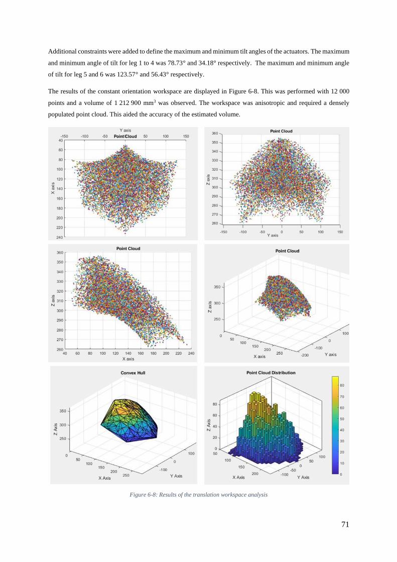
71
Additional constraints were added to define the maximum and minimum tilt angles of the actuators. The maximum
and minimum angle of tilt for leg 1 to 4 was 78.73° and 34.18° respectively. The maximum and minimum angle
of tilt for leg 5 and 6 was 123.57° and 56.43° respectively.
The results of the constant orientation workspace are displayed in Figure 6-8. This was performed with 12 000
points and a volume of 1 212 900 mm3 was observed. The workspace was anisotropic and required a densely
populated point cloud. This aided the accuracy of the estimated volume.
Figure 6-8: Results of the translation workspace analysis

72
Xiaolong et al. [90] designed a redundant actuated 5-DOF PKM which displayed a similar point cloud, shown in
Figure 6-9. This served as a validation that the constraints imposed were correct.
Figure 6-9: Workspace results that was obtained by Xialong et al. [90].
6.3.3 Alpha Rotation and Translational Workspace
The PKM constraints for alpha rotation with translation are shown in Table 6-2. The tilt angle constraints for the
actuators are the same as for the constant orientation workspace. A noticeable difference for the alpha rotation
with translation to the constant orientation workspace is that it loses a DOF along the x axis and the x value
remained at 113.31 mm. This meant that the alpha rotation with translation only occurs about a plane. Poses and
conditions depicting the alpha maximum and minimum angles of tilt is illustrated in Appendix G.1.
Table 6-2: PKM constraints for alpha rotation
Axes Value Reason for limitation
X value 111.31 mm Translation along the x axis is lost.
Y minimum 136.12 mm Maximum stroke length of actuator 3 and 4.
Y maximum -136.12 mm Maximum stroke length of actuator 1 and 2.
Z minimum 262.08 mm Maximum stroke length for actuator 1 – 4.
Z maximum 356.68 mm Maximum stroke length of actuators.
α minimum -35.73° Maximum stroke length of actuator 2 and actuator 5
α maximum 35.73° Maximum stroke length of actuator 4 and actuator 6
The results of the alpha rotation with translation workspace is depicted in Figure 6-10. This was performed with
12 000 points and the resulting area was 18112 mm2. The boundary function was used since the convex hull
surface wrap is used for 3D volumes.

73
Figure 6-10: Alpha rotation and translational workspace
6.3.4 Beta Rotation and Translational Workspace
Table 6-3 presents the position and orientation limits of the end effector when undergoing beta rotation and with
translation. The poses performing the maximum and minimum beta rotations are shown in Appendix G.2. The tilt
angle constraints for the actuators are the same as for the constant orientation workspace.
Table 6-3: Limits for the beta workspace analysis
Axes Value (mm) Reason for limitation
X minimum 46.50 Self-clashing.
X maximum 239.50 Self-clashing.
Y minimum 136.12 Maximum stroke length of actuator 3 and 4.
Y maximum -136.12 Maximum stroke length of actuator 1 and 2.
Z minimum 252.07 Self-clashing.
Z maximum 356.68 Maximum stroke length of actuators.
β minimum -36.8° Self-clashing.
β maximum 27.17° Self-clashing.
Figure 6-11 displays the workspace of the end effector for beta rotation with translation. The simulation was
performed with 12 000 points and a volume of 2 022 000 mm3 was obtained. The workspace volume was far
greater than the workspace obtained for constant orientation and was therefore investigated for sources of errors.

74
The yellow portion highlighted on the xz plane indicates a region that the robot cannot physically move to due to
self-clashing. An example of this is shown in Figure 6-12. The points were plotted due to MATLAB® not
possessing a constraint equation to limit this movement. The limitation for this joint can be addressed in future
research. To adequately understand the machine’s limits, the SolidWorks® model should be consulted and the
PKM can be restrained through mates. Therefore, the problem can be solved through manipulation in a 3D CAD
package. Translating the constraint mathematically should be addressed in future work. The volume generated is
therefore an overestimation of the machine’s workspace for beta rotation with translation.
Figure 6-11: Beta rotation and translational workspace

75
Figure 6-12: A physically impossible pose
6.3.5 Maximal Workspace Excluding Parasitic Motion
The maximal workspace considers all points that can be reached by the end effector in at least one orientation.
Each of the workspace MATLAB® scripts (constant orientation, alpha rotation with translation and beta rotation
with translation) were run with 4 000 points and were combined into a matrix. The points within the final matrix
were then plotted as depicted in Figure 6-13. The overestimation of volume from the beta rotation with translation
is present in this analysis as indicated on the xz plane with the yellow highlight. The volume produced from
MATLAB® was 2 120 000 mm3. This result illustrates the correct employment of combining all valid points into
a common matrix since the maximal workspace was the largest recorded workspace and is congruent with its
definition.
Joint rotations
that require
rotational limits

76
Figure 6-13: Maximal workspace of the PKM
6.3.6 Inclusive Orientation Workspace
For the inclusive orientation, the simulations were run for alpha and beta orientations that ranged from 8° up to
and including 10°. The alpha rotation with translation and beta rotation with translation was plotted with 5 000
points each and all valid points were merged into a common matrix. The results of the inclusive orientation
workspace are shown in Figure 6-14. The volume obtained was 804 710 mm3. The inclusive orientation volume
was the smallest volume obtained thus validates the approach.

77
Figure 6-14: Inclusive orientation workspace for angles ranging from 8° up to and including 10°
6.3.7 Constant Orientation Workspace Height Investigation
The constant orientation workspace height was chosen to be investigated and this approach can be used for other
workspaces. The height ranged from 262.08 mm up to and including 356.68 mm. The workspace was sliced at
263 mm and continued in 10 mm increments up to 353 mm. The last slice was taken at a height of 356 mm. Figure
6-15 depicts each of the planes but they are not displayed with the same scale. The height investigation was done
for the purpose of presenting the change of shape of the workspace with a change in height. The correct scale of
each slice is illustrated Figure 6-16. The following insights are deduced from Figure 6-15 and Figure 6-16:
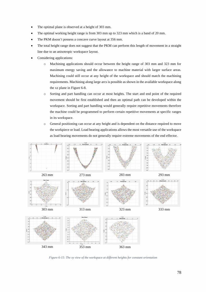
78
• The optimal plane is observed at a height of 303 mm.
• The optimal working height range is from 303 mm up to 323 mm which is a band of 20 mm.
• The PKM doesn’t possess a concave curve layout at 356 mm.
• The total height range does not suggest that the PKM can perform this length of movement in a straight
line due to an anisotropic workspace layout.
• Considering applications:
o Machining applications should occur between the height range of 303 mm and 323 mm for
maximum energy saving and the allowance to machine material with larger surface areas.
Machining could still occur at any height of the workspace and should match the machining
requirements. Machining along large arcs is possible as shown in the available workspace along
the xz plane in Figure 6-8.
o Sorting and part handling can occur at most heights. The start and end point of the required
movement should be first established and then an optimal path can be developed within the
workspace. Sorting and part handling would generally require repetitive movements therefore
the machine could be programmed to perform certain repetitive movements at specific ranges
in its workspace.
o General positioning can occur at any height and is dependent on the distance required to move
the workpiece or load. Load bearing applications allows the most versatile use of the workspace
as load bearing movements do not generally require extreme movements of the end effector.
Figure 6-15: The xy view of the workspace at different heights for constant orientation
263 mm 273 mm 283 mm 293 mm
303 mm 313 mm 323 mm 333 mm
343 mm 353 mm 363 mm

79
Figure 6-16: Isometric view of slices of the constant orientation workspace at different heights
6.4 Chapter Summary
This chapter described the singularities and workspace analysis. The different types of singularities were
discussed and 3 singularity poses were discovered by observation. The different types of workspace were
discussed. The Monte Carlo method, convex hull and point cloud distributions using histograms were generated
through MATLAB®. The workspace analysis was an extension the inverse kinematic analysis documented in
Section 5. The following workspace volumes were achieved:
• Constant orientation: 1 212 900 mm3
• Alpha rotation with translation 18112 mm2 (area)
• Beta rotation with translation 2 022 000 mm3
• Maximal workspace excluding parasitic motion 2 120 000 mm3
• Inclusive orientation workspace 804 710 mm3
The following chapter presents the electronic and software system. The selected components are discussed and
wiring diagrams are presented. The development of a control box is documented. The software system used to
automate the protype is presented and a flow diagram of the integration of the electronic and software system with
the prototype is documented.

80
7. ELECTRONIC AND SOFTWARE SYSTEM
7.1 Introduction
An electronic and software system was designed to automate the motion of the PKM and considered the following
design aspects:
• Low cost: The research aimed to produce a low-cost desktop prototype through AM.
• Mobile: Electronic hardware must be portable.
• Compact: The electronic hardware must be enclosed in a control box with the allowance for airflow
through the control box to allow for cooling of the electronic hardware.
• Aesthetic: The control box must be aesthetically pleasing.
7.2 Flow Diagram of System
Figure 7-1 shows the flow diagram for the electronic hardware. The diagram only represents the connection to
one actuator for simplicity. Appendix E presents the cost of the electronic components.
Figure 7-1: Flow Diagram of Electronic Hardware
7.3 Description of Selected Components
7.3.1 Motor Selection
Stepper motors were selected in the development of the prototype due to their high positioning capability and
range of motion. The disadvantage of the stepper motor was its application as an open loop system. NEMA 11,
17, and 23 stepper motors were applicable. The NEMA 17 stepper motor was the most cost effective from the
available stepper motors. The NEMA 17 stepper motors were more compact than the NEMA 23 stepper motors
therefore aiding the development of a compact prototype. The torque capability of the stepper motors did not
influence the selection of the stepper motors since the prototype was aimed to demonstrate the potential use in
machining, part handling, sorting and general positioning applications. The payload test in Section 8.7
demonstrated the payload capability although the PKM was not designed toward a payload specification and was
tested until failure.
NEMA 17 Stepper motors were selected. Four 42BYGHW609 stepper motors and two 42BYGHM809 stepper
motors were used and possessed 1.8 degrees/step and 0.9 degrees/step, respectively. The motors had a 1.7A rating.
A test was carried out to determine which wires of the stepper motors belonged to the same coil. A multimeter
was used to test the resistances between the various wires. The value of 1 represents a finite resistance measured
between the two wires suggesting they belong to the same coil. The value of 0 represents an infinite resistance
230 V
PC
Power
Supply
Stepper Motor
Driver
Arduino
Stepper
Motor Actuator

81
(no connection) between the two wires meaning they do not belong to the same coil. Pulse Width Modulation
(PWM) energizes the coils with signals sent from the microcontroller and stepper motor driver. Table 7-1 displays
the pairs of wires that belong to the same coil. All six stepper motors displayed the same results shown in Table
7-1. Open Impulse and Longway Motor [141-143] provides the technical specifications of the stepper motors.
Table 7-1: Determining the wire pairs for the stepper motors
Green Blue Black Red
Green - 0 1 0
Blue 0 - 0 1
Black 1 0 - 0
Red 0 1 0 -
7.3.2 Stepper Motor Drivers
Stepper motors can be controlled by a range of stepper motor drivers. The M860H, DM542, TB6600 and TB6560
stepper motors drivers were considered. The TB6560 was selected as it was the most cost-effective and compact.
A disadvantage of the TB6560 is that it not as robust as other stepper motor drivers but the TB6560 was designed
to be housed within a control box as presented in Section 7.5. The TB6560 has 14 different amperage outputs,
which are set using switches 𝑆𝑊1, 𝑆𝑊2, 𝑆𝑊3 and 𝑆1. The decay setting is set with switch 𝑆2 and refers to the
amperage delivered when the motors static. The driver can accomplish microstepping with switch 𝑆3 and 𝑆4.
The decay setting relates to how the stepper motor is switched off. The switches 𝑆5 and 𝑆6 control the decay
setting and this determines how fast the motor decelerates to a stop. Fast decay refers to a fast deceleration of the
motor and is applicable for low speeds and vice versa. Figure 7-2 displays the TB6560 stepper driver. DIY
Electronics [144] provided the technical specifications of the TB6560 stepper motor.
Figure 7-2: The TB6560 stepper motor driver
7.3.3 Microcontroller Board Layout and Selection
The operating voltage of the Arduino Mega 2560 is 5V. The Arduino Mega was more cost-effective than the
Arduino Due and it does not have interfacing challenges with peripheral components as faced by the Arduino
Due. The Arduino Mega was selected and had atleast 12 PWM ports, which was sufficient for this research. The
Arduino Uno was more cost-effective and compact but only possessed 6 PWM ports which hindered it use. Figure
7-3 [145] depicts the schematic diagram of the Arduino Mega indicating the PWM ports. Mantech [146] provided
the technical specifications of the Arduino Mega 2560.
Signal setting
combinations

82
Figure 7-3: Schematic Diagram of the Arduino Mega [145]
7.3.4 Power Supply
Two Mean Well S-320-24-D power supplies were chosen to power the TB6560 stepper motor drivers. The motor
drivers required 10V to 35V to be powered thus a 24V power supply was selected. The motor drivers required 3A
each thus, one power supply unit could supply 3 motor drivers with current since it is rated at 12.5A. An attractive
feature was the built-in cooling fan which aided in its selection. Figure 7-4 depicts the power supply. The power
supply is powered by 230V from a wall socket. Mouser Electronics [147] provided the technical specifications of
the power supplies.
Figure 7-4: Mean Well S-320-24
7.3.5 Sensor Selection
This research used the OCM as a low-cost displacement sensor. One of the advantages of the optical mouse is that
it is readily interfaced with the computer and is cost effective. Some of the disadvantages are that the mouse needs
to translate along a plane or flat surface to avoid errors. The user needs to test the mouse experimentally to obtain
an acceptable resolution. Laser and draw wire sensors were considered with data acquisition hardware and
software. Laser and draw wire sensors possess advantages such as high-resolution measuring capabilities, ease of
data acquisition and data analysis. However, the laser and draw wire sensors are high in cost especially when
multiple sensors are required. The data acquisition hardware and software units are expensive and generally cannot
be easily interfaced with sensors from other suppliers hence the selection of the OCM sensor. Other cost-effective
sensors such as infrared and ultrasonic sensors possessed low-resolution measuring capabilities and were not
suitable for this research.
a. b.

83
Bachraty and Zalman [148] investigated using the optical mouse as a 2D position sensor. The ADNS6010 sensor
was tested and noted that parameters such as the interacting surface, sensor acceleration and sampling rate affects
the accuracy of the mouse. Bonarini et al. [149] used a pair of optical mouse sensors for dead reckoning of mobile
robots. Ng [150] used the mouse sensor as a 2D displacement sensor to measure the viscoelastic elongation of
polyethylene. The mouse could not operate if the distance between the object and itself was larger than 1.25 mm.
Wang [151] used a mouse sensor for tactile sensing in conjunction with MATLAB®. The mouse produced
accurate measurements with sub-millimeter resolution for slow displacements. Figure 7-5 depicts an HP M-
UAE96 mouse. The optical mouse was used in conjunction with MATLAB®.
Figure 7-5: The optical mouse sensor selected
7.4 Wiring Diagrams
Figure 7-6 shows the wiring scheme used for the electronic system. Figure 7-7 shows a close-up view of the
wiring scheme for one stepper motor.

84
Figure 7-6: Wiring diagram of the electronic system
Figure 7-7: Close-up wiring diagram of a stepper motor to a TB6560 Stepper motor driver [152]

85
7.5 Control Box
Figure 7-8 shows the SolidWorks® assembly and the physical construction of the control box. The stepper motors
were connected to microphone 5-P-in-line sockets with matching plugs. The power supplies were mounted on its
side and the motor drivers were mounted upright into an additive manufactured casing. Spacing strips were
produced through AM to stabilise and mount the power supplies to the control box. The advantages of this
arrangement are that the motor drivers are positioned ideally such that air flows through the fins and the row of
motor drivers was positioned close to the fan. The power supply fans exhaust air inward towards the box and the
suction fan draws out the heat generated. This arrangement also allowed more space for wiring and facilitated the
removal of electrical hardware without disconnecting many components. The disadvantages were that wiring was
a challenge for motor drivers furthest away from the power supply outputs.
Figure 7-8: The SolidWorks® model and fully assembled control box
a. The SolidWorks® Assembly.
b. The control box fully assembled.
7.6 Software System
SolidWorks® provided reference points for the inverse and forward kinematic analyses for MATLAB®. All
mathematical analyses were performed using MATLAB®. Simulink was used to create the inverse kinematic
block diagram and verify the MATLAB® scripts which performed the inverse kinematic calculations.
Arduino Integrated Developmental Environment (IDE) software served as the platform to program the stepper
motors. All steppers were moved simultaneously by using the AccelStepper and MultiStepper libraries. The
Mulistepper code was sensitive to the pin specification. Figure 7-9 illustrates how different software and electronic
system are related to each other and other aspects of the project.
a. b.

86
Figure 7-9: The integration of the electronic and software system with the prototype
Simulink can be used to send pulses to the stepper motor as an alternative to the Arduino IDE software. Figure
7-10 displays the Simulink model used to test the connection between Simulink and the Arduino board. The
Arduino IDE software was preferred.
SolidWorks® 3D CAD Model
End effector pose parameters: x, y, z, alpha beta
MATLAB® inverse kinematics script file
Number of steps required for stepper motors to turn
Arduino IDE
Arduino Mega 2560
Stepper motor drivers
Stepper motors
Linear actuators
Physical movement of PKM
Virtual movement of PKM
SolidWorks® measuring tool
Manual transfer
MATLAB® command window output
Manual transfer
PC signal
Arduino signals
Stepper motor driver signals
Rotational input to linear actuators
Movement of actuators

87
Figure 7-10: A typical Simulink model that can be used communicate with an Arduino board
7.7 Chapter Summary
This chapter described the design requirements for the electronic and software design. A flow diagram was
developed to indicate the relationship between the different electronic hardware. The components of the electronic
system were described and the use of an optical mouse as a low-cost position sensor was presented. The control
box was documented. The chapter concluded with a description of the software system.
The following chapter presents the system performance and testing. Simulations and physical testing were
conducted on the prototype. Physical tests such linear actuator accuracy and repeatability, PKM accuracy and
repeatability and payload tests are presented. Simulations were carried out on the inverse and forward kinematic
analyses using SolidWorks® and MATLAB®.

88
8. SYSTEM PERFORMANCE AND TESTING
8.1 Introduction
This chapter documents the simulations and physical testing. The linear actuators were tested to determine the
accuracy and repeatability of each of them. This was conducted to determine sources of error. Simulations were
conducted on the inverse kinematics to validate the inverse kinematic equations developed with MATLAB® script
files with reference to the SolidWorks® model. Testing was conducted on the physical model to investigate
accuracy and repeatability in terms of the inverse kinematics. The inverse kinematic analysis was used to perform
payload testing on the PKM to investigate the relationship between load and leg actuation accuracy and to
determine the maximum payload that the PKM could lift. Simulations were conducted to determine the accuracy
of the forward kinematic equations developed with MATLAB® script files with reference to the SolidWorks®
model. Further simulations were conducted to determine if the guess deviations influenced the number of
iterations in accordance with the NR method. Another aim of this experiment was to determine the sensitivity of
each variable to guess deviations and convergence.
8.2 Testing System
The testing system was designed to measure the accuracy and repeatability. The OCM was investigated and used
as a low-cost displacement sensor with an advantage of being readily interfaced with a computer. MATLAB®
was used to acquire data. PG 30 aluminium profile was used to build a frame around the PKM for the mounting
of sensors and shaft supports. 90° angled supports were used to mount the aluminium profiles to the wooden base.
Wooden inserts were fixed into the wooden base, which allowed the 90° support brackets to be fastened to the
base. Appendix E shows the cost of the materials and components.
8.2.1 Translation Testing System Figure 8-1 (a) depicts the testing system to test the translational movement of the end effector. Two computer
mouses were used. One mouse was mounted vertically (z-direction measurement) and the other mouse was
mounted to the end effector (x and y-direction measurement) with a connecting bracket shown in Figure 8-2 (c).
The mouse tracking z-direction movements were mounted onto a wooden platform, using the component shown
in Figure 8-2 (b) and both OCM sensors were mounted within the brackets illustrated in Figure 8-2 (a). The
wooden platform moved vertically along stainless-steel shafts with linear bearings. The specifications for the
linear bearings are provided by Precision Bearing House [153].
The OCM needed to move along a flat surface to output readings. The reverse side of a mirror was used because
it possessed a matte finish allowing the OCM to log accurate data. A mirror was also used since it has a smooth
surface and the mirror would not bend. The vertical OCM moved passively as the wooden platform is pushed up
or lowered by the end effector.
The OCM is sensitive to inconsistent movements and could output inaccurate readings therefore the wooden
platform was designed to run along linear shafts with linear bearings. The linear shafts were fastened with shaft
supports to the aluminium profiles. The mirror was fastened onto two pairs of linearly adjustable brackets. The
pairs of adjustable brackets allowed the mirror to be positioned to make the appropriate contact with the OCM.

89
8.2.2 Rotation Testing System The OCM could not measure tilt and the testing system was altered and is shown in Figure 8-1 (b). The component
is shown in Figure 8-2 (d) was attached to the end effector. A mirror was also attached to the top of the component
to replicated the tilt angle of the end effector. A digital Vernier calliper was used to measure the angle of tilt
through the gradient formula. A horizontal level (layer) was designed such that a measuring bracket could be
mounted onto it. The horizontal level assisted in recording z displacements from the same height consistently and
the measuring bracket was designed with predefined hole spacings.
Figure 8-1: Testing system designs for translation and rotation
a. Testing system for translational testing
b. Testing system for rotational testing
Figure 8-2: Mouse and end effector attachments
a. The OCM mounting bracket
b. Bracket connecting the OCM to the wooden platform
c. Component connecting the end effector to the OCM mounting bracket
d. Component connecting the mirror to the end effector
a. b.
a. b.
c. d.

90
8.3 Method of Calibration
The PKM was calibrated before every test. The stroke length of each actuator influenced the position and
orientation of the end effector. A manual method was used to calibrate the PKM, whereby the stroke length of the
actuator was measured with a digital Vernier calliper. The difference between the measured stroke length and a
stroke length of 5 mm was converted into steps for the stepper motor. The signal was sent to the stepper motor
and then the linear actuator was calibrated. This was done for each actuator. Figure 8-3 shows the method of
measuring the stroke length of an actuator.
Figure 8-3 Calibration of an actuator
8.4 Linear Actuator Accuracy and Repeatability
8.4.1 Aim
This experiment aimed to determine the accuracy and repeatability of each linear actuator.
8.4.2 Apparatus
• Digital depth gauge Vernier Calliper
• Aluminium extruded profiles
• Desktop computer
• Arduino IDE software
• Linear actuators
8.4.3 Methodology
The test followed the steps below:
1. Remove all revolute joints from the back of the motors.
2. Mount a horizontal beam (aluminium profile) across one side of the testing frame as displayed in Figure
8-5 (a).
3. Place all actuators underneath the aluminium horizontal beam as shown in Figure 8-5 (a).
4. Calibrate the digital depth gauge Vernier calliper using a flat granite table, as illustrated in Figure 8-4.

91
5. Place the digital depth gauge Vernier calliper onto the horizontal beam and record the initial distance to
the top of the actuators.
6. Switch on the actuators using the Arduino IDE and set each actuator to move 10 mm.
7. Record the final distance to the top of the actuators, as depicted in Figure 8-5 (b).
8. Repeat steps 5 to 7 until 10 readings are obtained for an actuation distance of 10 mm.
9. Repeat steps 5 to 8 for actuation distances of 20 mm, 30 mm, 40 mm and 50 mm.
Figure 8-4: Calibration of the digital depth gauge Vernier Calliper
Figure 8-5: Set-up and measurement of actuator lengths
a. The set-up of the linear actuators under the horizontal aluminium profile.
b. Placement of the Vernier calliper on the horizontal aluminium profile and measuring the distance to the
top of the actuators.
8.4.4 Results
The repeatability and accuracy of the linear actuators were calculated using the formulae for robot accuracy and
repeatability, as described by Groover [154]. Control Resolution (CR) is defined as the smallest possible
addressable point that can be manipulated over a range of motion. The 𝐶𝑅 is dependent on the electromechanical
a. b.

92
components and the controller of the robot. This research used electromechanical 𝐶𝑅 and is calculated in Equation
8.1. Other related calculations are presented in Appendix C.2.
𝐶𝑅 =
𝑝𝑖𝑡𝑐ℎ 𝑜𝑓 𝑡ℎ𝑟𝑒𝑎𝑑𝑒𝑑 𝑟𝑜𝑑
𝑠𝑡𝑒𝑝𝑠/𝑟𝑒𝑣 𝑜𝑓 𝑠𝑡𝑒𝑝𝑝𝑒𝑟 𝑚𝑜𝑡𝑜𝑟=
1.25 𝑚𝑚
200= 0.00625 𝑚𝑚/𝑠𝑡𝑒𝑝
(8.1)
The 𝐶𝑅 for actuator 1 to 4 was 0.00625 mm/step. Actuators 5 and 6 used stepper motors that performed 400
steps/revolution; therefore, the 𝐶𝑅 for these actuators was 0.003125 mm/step.
The accuracy and repeatability formulae are noted below in Equation 8.2 and 8.3 [154].
𝑅𝑒𝑝𝑒𝑎𝑡𝑎𝑏𝑖𝑙𝑡𝑦 = ±3𝜎
(8.2)
𝐴𝑐𝑐𝑢𝑟𝑎𝑐𝑦 =
𝐶𝑅
2+ 3𝜎
(8.3)
Table 8-1 summarises the accuracy and repeatability of all the actuators. This was conducted to find sources of
error when the PKM is tested with all actuators moving simultaneously. Figure 8-6 depicts the relationship
between the actuation distance and standard deviation. The data obtained from testing is presented in Appendix
A.1.
Table 8-1: Accuracy and repeatability of actuator 1 to 6
Actuator Repeatability (mm) Accuracy (mm)
1 0.18 0.19
2 0.12 0.12
3 0.13 0.13
4 0.14 0.14
5 0.12 0.12
6 0.20 0.20
Figure 8-6: Graph of standard deviation versus actuation length
0
0,02
0,04
0,06
0,08
0,1
0,12
0 10 20 30 40 50 60
Stan
dar
d D
evia
tio
n (
mm
)
Actuated Distance (mm)
Standard Deviation vs Distance
Actuator 1 Actuator 2 Actuator 3 Actuator 4 Actuator 5 Actuator 6

93
8.4.5 Analysis
The linear actuators, though constructed mainly through AM, exhibits readings that were accurate to a tenth of a
millimeter in most cases. The accuracy and repeatability, calculated from the formulae given by Equation 8.1 to
8.3, showed that sub-millimeter movements could be attained. The accuracy and repeatability are acceptable since
the target specification for accuracy and repeatability was set to 2 mm. The values in Table 8-1 are well below the
target value therefore the actuators were permitted to be used for further testing. The graph of standard deviation
vs. actuation length showed that there is no pattern between the two variables. The actuator maintains its accuracy
and repeatability over different distances affirming its viability. The advantages of the conducted methodology
were the use of cost-effective equipment and short set-up time. One of the disadvantages of the employed
methodology was the repetitive manual measuring and data logging which was time-consuming. Another
disadvantage was the additional attention that was required to ensure the effective and accurate use of a digital
depth gauge Vernier calliper for reliable results. This process was also time-consuming.
8.4.6 Conclusion
The linear actuators proved to be suitable concerning accuracy and repeatability, with the most significant value
for both parameters being approximately 0.2 mm. The additive manufactured components were found to be
relatively accurate as a low-cost actuator and this validates the use of AM for prototyping. The linear actuators
were acceptable to be used for the position and orientation testing of the end effector.
8.5 Inverse Kinematic Analysis Simulations
8.5.1 Aim
To determine the accuracy of the inverse kinematic equations developed with MATLAB® script files with respect
to the SolidWorks® model.
8.5.2 Apparatus
• Desktop computer
• MATLAB® Software
• SolidWorks® Software
8.5.3 Methodology
The PKM was designed and developed in SolidWorks® and could, therefore, be used as a reference to validate
the kinematic equations. MATLAB® script files were developed to theoretically calculate the length of each leg
for a particular position and orientation of the end effector. This approach was also used by Xu et al. [102] and
Zhang and Jing [155]. The region for testing points was divided into 5 regions as shown in Figure 8-7. Regions
are 55 mm in width along the y-axis. Table 8-2 summarizes the regions for sampling points to eliminate bias
sampling of randomly selected points.

94
Table 8-2: Regions for sampling testing points
Region Range of y values (mm)
1 −137.5 ≤ 𝑦 < −82.5
2 −82.5 ≤ 𝑦 < −27.5
3 −27.5 ≤ 𝑦 ≤ 27.5
4 27.5 < 𝑦 ≤ 82.5
5 82.5 < 𝑦 ≤ 137.5
Figure 8-7: The region of testing points. The regions are equally spaced along the y-axis
The methodology that was employed is listed:
1. Move the PKM in SolidWorks®
2. Record the position and orientation of the end effector
3. Record the leg length values from the virtual sensors in SolidWorks® for all six legs
4. Enter the end effector position and orientation values in the MATLAB® script file
5. Run the MATLAB® script file and record the calculated leg length values
6. Enter the end effector position and orientation values in Simulink
7. Run the Simulink model and record the calculated leg length values
8. Compare the values obtained from SolidWorks® to the values obtained from the MATLAB® script file
and Simulink.
8.5.4 Results
Ten points were tested in each region for the cases of translation, alpha rotation with translation and beta rotation
with translation. The results showed the largest deviation of 0.01 mm between the MATLAB® script file and
SolidWorks®. The errors between Simulink and SolidWorks® were the same as the errors observed in the
MATLAB® script file and SolidWorks®. Random points were selected in each region. The simulation results are
presented in Appendix A.2.

95
8.5.5 Analysis
The methodology employed to test the accuracy of the equations was time-consuming to transfer points between
SolidWorks® and MATLAB®. The errors observed are negligible and are due to rounding off errors. The spread
of points shows that the data used is unbiased and also proves that the machine’s theoretically position and
orientation are unaffected by its position in a specific region of its workspace. The advantage of the employed
methodology was that the kinematic equations could be verified before physical testing. This enabled the
movements of the prototype to be programmed as discussed in Section 8.6.
8.5.6 Conclusion
The method of validating the inverse kinematic equations was successful. The test also proved that the kinematic
equations were accurate. The errors observed were acceptable.
8.6 PKM Accuracy and Repeatability
8.6.1 Aim
This experiment aimed to investigate the accuracy and repeatability of the PKM.
8.6.2 Apparatus
• A digital Vernier calliper
• 2 Desktop computers
• Arduino IDE software
• MATLAB® software
• SolidWorks® software
• 2 OCM
8.6.3 Methodology
The test for the translational movement of the end effector followed the steps below:
1. Move the PKM in SolidWorks®.
2. Enter the coordinates of the end effector in MATLAB® to obtain the number of steps that the stepper
motor shaft needs to turn.
3. Enter the number of steps for the stepper motors in the Arduino IDE software.
4. Run the MATLAB® script file to track the position of the mouse on both computers and record the initial
pixel reading.
5. Upload the Arduino code to the Arduino microcontroller.
6. Record the final pixel readings from each computer when the PKM stops.
7. Reverse the sign of the steps that the stepper motors were required to execute to move it back to its home
position.
8. Upload the Arduino code to the Arduino microcontroller.
9. Repeat steps 3 to 8 until 10 movements are carried out to the same point.
10. Repeat steps 1 to 9 until 15 different points in the robot’s workspace have been tested.

96
The tests for the alpha and beta rotations of the end effector followed the steps below.
1. Move the PKM in SolidWorks®.
2. Enter the coordinates of the end effector in MATLAB® to obtain the number of steps that the stepper
motor shaft is to turn.
3. Enter the number of steps for the stepper motor to move in the Arduino IDE software.
4. Upload the Arduino code to the Arduino microcontroller.
5. Use the digital Vernier calliper to measure the depth at two different points using the measuring bracket.
6. Reverse the sign of the steps that the stepper motors were required to execute to move it back to its home
position.
7. Upload the Arduino code to the Arduino microcontroller.
8. Repeat steps 3 to 7 until 10 movements are carried out to the same point.
9. Repeat steps 1 to 8 until 15 different points in the robot’s workspace have been tested.
Figure 8-8 depicts the PKM performing translational motion. Figure 8-9 illustrates how two different depths were
measured to calculate the tilt of the end effector. Figure 8-10 shows the end effector performing a positive alpha
rotation. When the mirror was mounted onto the end effector with all actuators locked, the end effector could still
move due to the relatively large tolerances from additive manufactured plastic components. This allowed the end
effector to exhibit a tilt bias of -4° and this was accounted for when analysing the data for the beta rotation. Figure
8-11 shows the PKM with a tilt bias.
Figure 8-8: Testing the translational motion of the end effector.
a. The mouse tracking the x and y displacements of the end effector.
b. The mouse tracking the z displacement of the end effector.
a. b.
Wooden
platform
OCM
housing OCM
housing
Mirror

97
Figure 8-9: Measuring the angle of tilt for an alpha rotation.
a. Measuring depth 1 from the white bracket to the mirror
b. Measuring depth 2 from the white bracket to the mirror
Figure 8-10: The PKM performing a positive alpha rotation.
Figure 8-11: The tilt bias of the end effector when the mirror was placed on the end effector.
a. b.
-4°

98
Figure 8-12 depicts the SolidWorks® message that was displayed when all actuators were locked and the end
effector was attempted to be moved. The message confirmed that the end effector could not be moved
theoretically.
Figure 8-12: SolidWorks confirmation of no PKM movement when all actuators are locked.
8.6.4 Results
Accuracy and repeatability formulae used in the research were used by Zhao et al. [156] for the metrological
evaluation of a novel medical PKM developed. Other authors have used the formulae for accuracy and
repeatability analysis [157, 158]. The formulae are linked to ISO 9283: 1998 and are presented below. The
Position Accuracy (𝐴𝑃) is given by:
𝐴𝑃 = √𝐴𝑃𝑥
2 + 𝐴𝑃𝑦2 + 𝐴𝑃𝑧
2
(8.4)
𝐴𝑃𝑥 = �� − 𝑥𝑐
(8.5)
𝐴𝑃𝑦 = �� − 𝑦𝑐
(8.6)
𝐴𝑃𝑧 = 𝑧 − 𝑧𝑐
(8.7)
Where (��, ��, 𝑧) is the mean values or barycentre and (𝑥𝑐 , 𝑦𝑐 , 𝑧𝑐) is the commanded position.
�� =
1
𝑛∑(𝑥𝑗)
𝑛
𝑗=1
(8.8)
�� =
1
𝑛∑(𝑦𝑗)
𝑛
𝑗=1
(8.9)
𝑧 =
1
𝑛∑(𝑧𝑗)
𝑛
𝑗=1
(8.10)

99
Where(𝑥𝑗 , 𝑦𝑗 , 𝑧𝑗) is the coordinates of the reached point.
The Position Repeatability (𝑅𝑃) is given by:
𝑅𝑃 = 𝑙 + 3𝑆𝑙
(8.11)
𝑙 =
1
𝑛∑(𝑙𝑗)
𝑛
𝑗=1
(8.12)
Where 𝑙 is the mean value with respect to the deviations between the 𝑗𝑡ℎ reached positions.
𝑆𝑙 = √1
𝑛 − 1∑(𝑙𝑗 − 𝑙)2
𝑛
𝑗=1
(8.14)
Where 𝑆𝑙 is the standard deviation of the sample.
Table 8-3 and Table 8-4 presents the accuracy and repeatability results for translation. The tests were conducted
10 times for each point and a total of 15 different sample points were used. 3 points were used in each region. The
data obtained from testing is presented in Appendix A.3. The data obtained from the OCM testing is presented in
Appendix A.7. Appendix B.2 presents the Arduino code used for accuracy and repeatability testing.
Table 8-3: Accuracy results for translational motion.
Accuracy
Region - Point Entire PKM (mm) X axis (mm) Y axis (mm) Z axis (mm)
1-1 1.63 1.13 0.81 0.86
1-2 1.82 1.09 0.79 1.22
1-3 1.51 0.97 0.84 0.79
2-1 1.49 0.89 0.92 0.77
2-2 1.34 0.59 0.91 0.79
2-3 1.53 0.83 0.97 0.85
3-1 1.17 0.74 0.27 0.87
3-2 1.38 0.72 0.77 0.89
3-3 1.33 0.92 0.74 0.61
4-1 1.63 0.94 1.08 0.78
4-2 1.78 1.07 1.03 0.98
4-3 1.77 0.95 1.02 1.09
5-1 1.91 1.06 1.13 1.11
5-2 1.71 1.1 1.12 0.69
5-3 1.83 1.02 1.25 0.87

100
Table 8-4: Repeatability results for translational motion.
Repeatability
Region - Point Entire PKM (mm) X axis (mm) Y axis (mm) Z axis (mm)
1-1 2.71 2.16 1.92 1.73
1-2 2.29 2.02 1.61 1.11
1-3 1.56 0.78 1.54 0.82
2-1 1.96 1.61 1.42 0.72
2-2 2.51 2.01 1.81 1.17
2-3 1.62 1.49 0.62 1.33
3-1 2.51 2.64 0.46 1.67
3-2 2.67 1.85 0.76 2.42
3-3 2.56 2.43 2.09 1.03
4-1 1.78 1.69 1.37 0.8
4-2 2.2 1.8 1.84 1.66
4-3 2.33 1.69 1.7 1.05
5-1 2.05 1.53 1.49 1.33
5-2 1.67 0.75 1.53 0.6
5-3 2.48 1.87 2.45 1.02
Figure 8-13 shows a graphical representation of the results documented in Table 8-3 and Table 8-4.
Figure 8-13: Translational Accuracy and Repeatability vs. Y Displacement.
0
0,5
1
1,5
2
2,5
3
-150 -100 -50 0 50 100 150Acc
ura
cy a
nd
Rep
eata
bili
ty (
mm
)
Y Displacement of End Effector (mm)
Translation Accuracy and Repeatability vs Y Displacement
Accuracy Repeatability

101
The same sample size was used to test rotational performance. The graph of alpha rotation accuracy and
repeatability vs. alpha angle is given by Figure 8-14. Figure 8-15 shows the relationship between the alpha rotation
accuracy and repeatability and the y displacement.
Figure 8-14: Alpha Rotation Accuracy and Repeatability vs. Alpha Angle
Figure 8-15: Alpha Rotation Accuracy and Repeatability vs. Y Displacement
The graph of beta rotation accuracy and repeatability vs. beta angle is given by Figure 8-16. Figure 8-17 shows
the relationship between the beta rotation accuracy and repeatability and the y displacement of the end effector.
0
0,5
1
1,5
2
-25 -20 -15 -10 -5 0 5 10 15 20 25
Acc
ura
cy a
nd
Rep
eata
bili
ty (
mm
)
Alpha Angle (Degrees)
Alpha Rotation Accuracy and Repeatability vs Alpha Angle
Accuracy Repeatability
0
0,2
0,4
0,6
0,8
1
1,2
1,4
1,6
1,8
2
-100 -50 0 50 100 150
Acc
ura
cy a
nd
Rep
eata
bili
ty (
mm
)
Y Displacement of End Effector (mm)
Alpha Rotation Accuracy and Repeatability vs Y Displacement
Accuracy Repeatability

102
Figure 8-16: Beta Rotation Accuracy and Repeatability vs. Beta Angle
Figure 8-17: Beta Rotation Accuracy and Repeatability vs. Y Displacement
8.6.5 Analysis
Figure 8-13 shows a relationship between the translation accuracy and the y-direction. This indicates that accuracy
is anisotropic. The PKM is most accurate when the y-displacement is low and loses accuracy as the y displacement
increases. The accuracy deviations are magnified through the use of an additive manufactured desktop model. The
tolerances of plastic joints are not as high nor as rigid as metal mechanical joints. The accuracy ranged from 1.17
mm to 1.91 mm. This is acceptable and was below the target specification of 2 mm.
0
0,2
0,4
0,6
0,8
1
1,2
1,4
1,6
1,8
2
-20 -15 -10 -5 0 5 10 15 20
Acc
ura
cy a
nd
Rep
eata
bili
ty (
mm
)
Beta Angle (Degrees)
Beta Rotation Accuracy and Repeatability vs Beta Angle
Accuracy Repeatability
0
0,2
0,4
0,6
0,8
1
1,2
1,4
1,6
1,8
2
-150 -100 -50 0 50 100 150
Acc
ura
cu a
nd
Rep
eata
bili
ty (
mm
)
Y Displacement of End Effector (mm)
Beta Rotation Accuracy and Repeatability vs Y Displacement
Series1 Series2

103
The results of the translational repeatability did not show any relationship to the displacement along the y-
direction. The repeatability results were erratic, as shown in Figure 8-13. This is due to the high sensitivity OCM
sensors and it encountering noise since it was used on a robotic system that vibrates. The repeatability of the
translational movement ranged from 1.56 mm to 2.71 mm. This indicates the large variances encountered when
using OCM sensors as low-cost displacement sensors. The formulae used to calculate repeatability included a
standard deviation calculation which resulted in the repeatability values being sensitive to variance in pixel
measurements. The pixel data obtained from the measurements contained a few outliers which produced relatively
high repeatability values. The OCM sensors provide more accurate results when many iterations of the movement
to the same point are conducted due to the relatively high variance observed. For this reason, 10 iterations were
conducted per point. Most of the repeatability values were more than 2 mm which exceeded the target specification
of 2 mm. The repeatability was therefore larger than the accuracy due to the high sensitivity of the OCM sensors
and outliers in the pixel measurements.
For the rotational analysis, the accuracy and repeatability were measured against the angle of rotation and the y
displacement. The alpha accuracy displayed a similar pattern as to the translational accuracy. The accuracy was
high for small y displacements but the PKM lost accuracy as it moved further along the y-direction. The weight
of the PKM itself tends to magnify the loss of accuracy as the machine moves towards extreme points along the
y-direction. The accuracy ranged from 0.26° to 1.74°. This was acceptable as it is lower than the target
specification of 2°. There was no evident relationship between accuracy and rotation angle. The repeatability of
the alpha rotation showed a relationship with the angle of rotation. The larger the angle of rotation, the poorer the
repeatability. The repeatability ranged from 0.23° to 1.9° which was below the target specification of 2°. There
was no correlation found between the alpha rotation repeatability and y displacement. Figure 8-14 and Figure 8-15
illustrate the insights.
The beta rotation results illustrated the same patterns as the alpha rotations. The beta rotation accuracy was
dependent on the y displacement of the end effector whereby the larger the y displacement, the poorer the
accuracy. The accuracy ranged from 0.21° to 1.76°. The repeatability was dependant on the angle of rotation such
that high repeatability was observed for small angles of rotation. The repeatability ranged from 0.28° to 1.33°.
Both the accuracy and repeatability observed were smaller than the target specification. Figure 8-16 and Figure
8-17 illustrates the described relationships.
The methodology was time-consuming. Many machine movements were conducted which was tiresome through
manual measurements and data logging. Another disadvantage was that 3 software programs were required to
conduct each movement. Advantages of the methodology were the cost-effective equipment that were used and
no additional software was required from the institution to conduct the tests except for the Arduino IDE which
was free.
8.6.6 Conclusion
The accuracy and repeatability of the PKM were smaller than the target specifications of 2 mm and 2°. The only
exception was repeatability of the translational movement which showed most of the repeatability results to have
exceeded 2 mm. The use of a digital Vernier calliper produced better results in terms of the variance observed as
opposed to the OCM sensors. The tolerances in the plastic joints allow movement of the end effector when all

104
actuators are locked. The PKM also incurred a tilt bias about the y-axis when the mirror was attached to the end
effector.
8.7 Payload Testing
8.7.1 Aim
This experiment aimed to investigate the relationship between load and leg actuation accuracy and to determine
the maximum payload that the PKM could lift.
8.7.2 Apparatus
• Digital scale
• Digital Vernier Calliper
• Calibrated weights
• Desktop computer
• Arduino IDE software
8.7.3 Methodology
The test followed the steps below:
1. Validate the mass of each calibrated disc with the digital scale.
2. Position the PKM in SolidWorks® such that the end effector does not move in the x and y directions,
thus only performing the vertical motion.
3. Set the corresponding number of steps to turn for each stepper motor.
4. Load the PKM.
5. Run the Arduino code such that the end effector moves vertically upward.
6. When the PKM stops, measure all actuator legs using the Vernier Calliper.
7. Return the PKM to its home position.
8. Repeat steps 4 to 7 for different weights.
Figure 8-18 shows the validation of a 1-pound mass. All weighted discs were placed on the scale and validated
before loading the PKM with the various weights.
Figure 8-18: Mass validation of calibrated weights

105
8.7.4 Results
The leg lengths were measured with a digital Vernier calliper after each test under when the PKM was subjected
to various loads. Table 8-5 displays the largest actuation error recorded for each leg and the weight under which
the largest actuation error occurred. The results of this test can be found in Appendix A.4. Figure 8-19 depicts the
graph of mass versus leg actuation error. The results were plotted for each measured leg length for each load that
the PKM elevated. Figure 8-20 shows the PKM lifting various loads by a vertical distance of 50.42 mm.
Table 8-5: Summary of leg actuation errors as a function of load
Leg 1 Leg 2 Leg 3 Leg 4 Leg 5 Leg 6
Largest error (mm) 0.21 0.29 0.27 0.28 0.2 0.18
Load occurrence (kg) 7.09 7.09 7.09 12.07 8.44 5.27
Figure 8-19: Graph of Mass vs. Leg Actuation Error
Figure 8-20: The PKM lifting various weights vertically by 50.42 mm
a. The PKM lifting a load of 5.27 kg
b. The PKM lifting a load of 13.43 kg
c. The PKM lifting its maximum load of 25.23 kg
0
0,05
0,1
0,15
0,2
0,25
0,3
0,35
0 5 10 15 20 25 30Leg
actu
atio
n e
rro
r (m
m)
Mass (kg)
Mass vs Leg Actuation Error
Leg 1 Leg 2 Leg 3 Leg 4 Leg 5 Leg 6
a. b. c.

106
Figure 8-21 illustrates the components that failed. The PKM lifted a load of 25.23 kg. Upon reloading, at 25kg,
the mouse bracket and end effector failed.
Figure 8-21: Failed components after lifting a 25.23 kg load
a. Failure of the mouse bracket
b. Failure of the end effector
8.7.5 Analysis
The results from Table 8-5 shows the largest error of 0.29 mm at a load of 7.09 kg. The PKM lifted a mass of
25.23 kg at which the actuation error was smaller than 0.29 mm. Figure 8-19 shows that the actuation error and
mass have no relationship suggesting that the accuracy is independent of mass. The errors observed are accepted.
The errors obtained could also be attributed to human errors when using the digital Vernier calliper. Figure 8-20
shows that the load was placed directly above the PKM and not spread around the wooden platform for the purpose
of consistency of results and to replicate a point load as accurately as possible.
Figure 8-22 illustrates the joint at which failure occurred. The weakest point is at the revolute joints of the end
effector. This suggests that the additive manufactured components failed before the stepper motors could not push
a heavier load. Based on the power screw calculations and buckling calculations presented in Appendix C.1 and
C.3 respectively, the weakest element was the additive manufactured components. The advantage of the
methodology was that it was cost-effective with a short set up time. One of the disadvantages of the use of a
Vernier calliper and manual data logging was that the test was time-consuming. Manual loading and unloading of
weights could cause harm if not carried out appropriately. The point of failure of components caused the weights
to fall which could be dangerous if not carried out cautiously.
Figure 8-22: The weakest point of the PKM where the failure occurred.
a. b.

107
8.7.6 Conclusion
The results proved that leg actuation accuracy is independent of load. The PKM lifted the various loads with the
largest leg actuation error found to be 0.29 mm. This was acceptable. The PKM was able to lift a load of 25.23
kg. Improvements could be made to the design of the end effector to withstand a higher load. The weakest point
was found to exist at the actuator revolute joints linked to leg pair 1 and leg pair 2.
8.8 Forward Kinematic Simulations for Repeatability – MATLAB® and
SolidWorks®
8.8.1 Aim
To determine the accuracy of the forward kinematic equations developed with MATLAB® script files with respect
to the SolidWorks® model.
8.8.2 Apparatus
• Desktop computer
• MATLAB® Software
• SolidWorks® Software
8.8.3 Methodology
The test followed the steps below:
1. Set the mates that allow the end effector to move in translation only.
2. Move the end effector in SolidWorks®.
3. Record the end effector, theta and leg length values.
4. Input leg length data and relevant data into the forward kinematic script code in MATLAB®.
5. Record the converged values and the number of iterations.
6. Repeat steps 1 to 4 until 5 values are obtained from each region.
7. Repeat steps 1 to 5 for alpha rotation with translation and for beta rotation with translation.
8.8.4 Results
Points were taken from each region to eliminate the possibility of a biased data set. 25 points were obtained for
each of the cases tested. The results are presented in Table A.4 to Table A.6 in Appendix A.5.
8.8.5 Analysis
The greatest number of iterations observed for converged solutions was 8. Large initial guess deviations were
made in numerous cases and a solution was obtained. In certain instances, large initial guesses deviations caused
divergence. There were also cases when convergence occurred but not an incorrect value. This relates to the
unfeasible poses.
Concerning translation, the maximum initial guesses from the true position and orientation were 168.29 mm and
44.55° respectively. The largest convergence errors for position and orientation were 0.025 mm and 0.68 degrees
respectively. The alpha rotation with translation maximum initial guesses from the true position and orientation
was 101.31 mm and 43.79° respectively. The largest convergence errors for position and orientation were 0.04
mm and 0.09° respectively. The beta rotation with translation maximum initial guesses from the true position and

108
orientation was 167.33 mm and 73.57° respectively. The largest convergence errors for position and orientation
were 0.07 mm and 1.13° respectively.
The convergence errors are in the region of hundredths of a millimeter for translation. The orientation errors are
generally in the region of a tenth of a millimeter. There was an outlier observed of 1.13 mm orientation error. The
results showed a consistency of high accuracy irrespective of theoretical position.
The disadvantage of the methodology was that it was time-consuming due to the number of points tested and
manually transferring information across from SolidWorks® to MATLAB®. The methodology was advantageous
such that the forward kinematic equations could be verified through simulations before physical testing of the
prototype.
8.8.6 Conclusion
The NR method was successfully employed with high convergence accuracy for translation, alpha rotation with
translation and beta rotation with translation. The accuracy of the NR method is independent of position and
orientation. When convergence was observed, the number of iterations did not exceed 8 iterations.
8.9 Forward Kinematic Simulations – Guess Deviations Analysis
8.9.1 Aim
This investigation aimed to determine the sensitivity of each variable with respect to guess deviations from the
true value of the variable and convergence.
8.9.2 Apparatus
• Desktop computer
• MATLAB® Software
• SolidWorks® Software
8.9.3 Methodology
The test followed the steps below:
1. Set the mates that allow the end effector to move in translation only.
2. Move the end effector in SolidWorks®.
3. Record the end effector coordinates and the theta and leg length values.
4. Input leg length data and relevant data into the forward kinematic script code in MATLAB®.
5. Guess values close to the actual value and record the number of iterations.
6. Manipulate each variable by increasing the guess deviation of one variable at a time while holding all
other values to the values used in step 5. Record the number of iterations and check for convergence.
7. Repeat steps 1 to 6 for alpha rotation with translation and beta rotation with translation.
8.9.4 Results
The results of translation, alpha rotation with translation and beta rotation with translation have been split up into
graphs for position and for orientation because the guess deviation values used for the position have a larger range
than for rotation. The graphs for translation are illustrated in Figure 8-23 and Figure 8-24. Figure 8-25 and Figure

109
8-26 depict the results of alpha rotation with translation and finally Figure 8-27 and Figure 8-28 depict the results
of beta rotation with translation. Appendix A.6 presents the simulation results.
Figure 8-23: Translation Guess Deviation vs. Number of Iterations for position
Figure 8-24: Translation Guess Deviation vs. Number of Iterations for angular values
0
1
2
3
4
5
6
7
8
9
-300 -200 -100 0 100 200 300
Nu
mb
er o
f It
erat
ion
s
Guess Deviation
Translation:Guess Deviation vs Number of Iterations
X values Y Values Z values
0
2
4
6
8
10
12
14
16
-150 -100 -50 0 50 100 150
Nu
mb
er o
f It
erat
ion
s
Guess Deviation
Translation:Guess Deviation vs Number of Iterations
theta 1 theta 3 theta 5
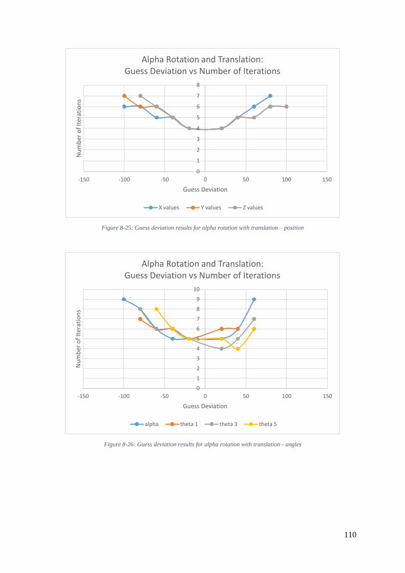
110
Figure 8-25: Guess deviation results for alpha rotation with translation – position
Figure 8-26: Guess deviation results for alpha rotation with translation - angles
0
1
2
3
4
5
6
7
8
-150 -100 -50 0 50 100 150
Nu
mb
er o
f It
erat
ion
s
Guess Deviation
Alpha Rotation and Translation:Guess Deviation vs Number of Iterations
X values Y values Z values
0
1
2
3
4
5
6
7
8
9
10
-150 -100 -50 0 50 100 150
Nu
mb
er o
f It
erat
ion
s
Guess Deviation
Alpha Rotation and Translation:Guess Deviation vs Number of Iterations
alpha theta 1 theta 3 theta 5

111
Figure 8-27: Guess deviation results for beta rotation with translation – position
Figure 8-28: Guess deviation results for beta rotation with translation - angles
8.9.5 Analysis
All graphs illustrate that as the guess deviation increases further away from the actual value, the solution
undergoes more iterations to converge. For translation, Figure 8-23 shows convergence for deviations up to 250
mm away from the actual value. The z value failed to converge and sometimes converged to an incorrect solution
when guesses were made between 150 mm and 250 mm lower than the true value. The z value was more sensitive
to deviations than the x and y values. The angular guesses for translation showed difficulty in convergence for
angular guesses greater than 20° from the true value but showed convergence for angles up to 100° less than the
actual value of the variables. Convergence also occurred in some cases where preceding guesses did not. These
observations show that reasonable guesses for the NR method are not symmetrical nor does it follow a predictable
pattern for a reasonable guess.
0
2
4
6
8
10
-300 -200 -100 0 100 200 300Nu
mb
er o
f It
erat
ion
s
Guess Deviation
Beta Rotation and Translation:Guess Deviation vs Number of Iterations
X values Y values Z values
0
2
4
6
8
10
-80 -60 -40 -20 0 20 40 60 80
Nu
mb
er o
f It
erat
ion
s
Guess Deviation
Beta Rotation and Translation:Guess Deviation vs Number of Iterations
beta theta 1 and 3 theta 5

112
The graphs relating to the alpha rotation with translation, illustrate that the position range for deviation was lower
than the translational case. Most iterations occurred with 4, 5 and 6 iterations. The angular guesses showed
convergence for the alpha guesses up to 100° less than the true value and guesses up to 60° greater than the actual
value. Other angular guesses showed convergence up to 80° less than the actual value and up to 60° greater than
the actual value. The theta 1 and theta 5 values are the most sensitive since the least number of convergence cases
occurred for these variables.
The graphs relating to the beta rotation with translation, Figure 8-27, show that most calculations were performed
in 5 iterations and z value is more sensitive to guesses less than the real value in comparison to the x and y values.
Concerning the angular guesses, most of the convergences also occurred with 5 iterations. The theta 1 and 3
variables were found to be most sensitive since convergence occurred the least number of times from the guess
deviation range. The beta and theta 5 variables displayed good convergence characteristics as convergence
occurred for all guess deviations ranging from 100° less and greater than the actual value.
The disadvantage of the test was that it required large amounts manual data logging and the transference of data
from SolidWorks to MATLAB® for each position and orientation of the end effector. The advantage of the test
was that it provided another validation of the forward kinematic equations and the effective use of the NR method.
8.9.6 Conclusion
Results showed that the number of iterations was dependent on guess deviation. This was observed for all cases
of the end effector’s movement and for all variables within each case. The result also showed that some variables
are more sensitive to guess deviation than to others. The range of the guess deviation is dependent on the type of
movement of the end effector. Convergence patterns are not symmetrical and sometimes convergence can occur
whilst preceding guess deviations do not bring about convergence. This suggests the unpredictability of a
convergence pattern in certain regions of a guess deviation.
8.10 Chapter Summary
Physical testing and simulations were conducted on various aspects, mainly centered around repeatability and
accuracy. Each of the individual tests documents the findings and conclusions drawn from each of the tests. The
key observations include:
• The novel inverse kinematic method consistently produced accurate results with errors in the range of
hundredths of a millimeter, mostly attributed to rounding off errors.
• The forward kinematic simulations yielded accurate results and conformed to the general patterns of the
NR method.
• A computer mouse can be used as a low-cost displacement sensor in conjunction with MATLAB®
yielding a resolution of 0.2 mm per pixel. The drawback is that it has a tolerance of 1.06 mm and
produced a large variance in pixels measured.
• The linear actuators, although produced through AM, possessed good accuracy and repeatability with
both parameters approximately 0.2 mm.

113
• The PKM produced acceptable accuracy and repeatability for translation, translation with alpha rotation
and translation with beta rotation. All results for accuracy and repeatability were smaller 2 mm and 2°
except for one case.
• The PKM loses accuracy as it moves further along in the positive or negative y-direction.
• Repeatability is dependent on the angle of rotation of the end effector.
• The PKM lifted a load of 25.23 kg. The failure occurred due to the strength of the additive manufactured
components.
The succeeding chapter presents the discussion for the conducted research. The research question, findings,
observations, performance and insights are discussed. The concept overview, justification and literature are
discussed. A discussion concerning the synthesis, design, singularities and workspace is presented. Physical
testing and performance of the PKM are discussed. The chapter also documents the implication of the PKM.

114
9. DISCUSSION
9.1 Chapter Introduction
The research question from Section 1.5 was: Can a novel PKM be developed for 3 translational and 2 rotational
DOFs to validate part handing, sorting, general positioning and robotic machining capabilities? This chapter
summarises the dissertation with the findings, observations, performance, and insights of the research while
addressing the research question. The implications of the novel PKM in the manufacturing sector are discussed.
9.2 Concept Overview, Justification and Literature
The growing inflation rate, weaker Rand and higher interest rates in South Africa inhibits entrepreneurship. South
Africa needs to remain technologically competitive and produce goods at a low cost and high quality. The BRICS
index of industrial production showed that South Africa has not significantly increased its industrial progress since
2014 [2]. Stats SA [7] showed that the manufacturing, mining and trade sectors underperformed for the first 3
months of 2019 with a contraction of 3.2%. South African Market Insights [159] revealed that the South African
manufacturing underutilisation had reached its highest percentage in 4 years with a value of 19.7%. This is due
mainly to insufficient demand suggested by a weak economy or increased imports. This identifies the need that
manufacturing machinery should be designed and produced within South Africa as opposed to being imported
which, in turn, creates job opportunities.
Researchers are exploring robotic platforms to perform tasks that were thought to be only possible with CNC
machines [15]. The drawbacks of CNC machines are that they are large, heavy and expensive [16, 17]. The
relatively low capital investment of robotic manipulators, reusability and flexibility, making them a suitable
alternative to CNC machines [18]. Robotic platforms have the potential to replace CNC machines for specific
tasks. PKM possesses a high payload to weight ratio, high stiffness and the errors of the joints are averaged.
PKMs, however, suffer from a relatively small workspace in comparison to serial manipulators. The selection of
the correct robotic platform is application-dependent. The workspace of a PKM can be designed to suit the needs
of the end-user [19]. PKMs have the potential to be designed, manufactured and implemented to assist the South
African economy.
PKMs that have been commercialised for dedicated machining tasks are large and heavy [8]. Other PKMs have
been commercialised but still, do not have the industrial presence as serial robots [11]. This establishes the need
for affordable robotic platforms. Industry 4.0 paradigms can be applied to robotic platforms to make them
technological relevant in the context of Industry 4.0.
Literature suggests that 2-DOF PKMs can perform either translational or rotational motion. Although possessing
more straightforward mathematical analyses, they lack the mechanical rigidity in comparison to PKMs with more
actuators. 2-DOF PKMs are designed for specific tasks that require a limited range of planar or spatial movements.
3-DOF can possess 2 translation and 1 rotation, 1 translation and 2 rotations, pure translations or pure rotations.
These motion capabilities produce a variety of architectural designs. The delta and spatial architectural type have
industrial presence. 3-DOF PKMs possessing pure rotations have not been adopted by industry as mainstream
mechanisms and lack mechanical rigidity.

115
Concerning 4-DOF PKMs, research suggests that the delta architectural type is the most commonly researched
and adopted by industry. The delta structure possesses low inertia since the motors are positioned at its footpoints
which enables high-speed pick and place applications. Many delta PKMs have been commercialised for pick and
place and AM applications. 4-DOF PKMs possess a larger workspace in comparison to 5-DOF and 6-DOF PKMs.
5-DOF PKMs have numerous architectural designs and unique machine structures in comparison to other DOF
PKMs. The most common motion combination is 3 rotational and 2 translational DOFs. It is uncommon for a 5-
DOF PKM to possess 2 rotational and 3 translations DOFs. The category of 5-DOF PKMs have received lesser
attention relative to 3-DOF, 4-DOF and 6-DOF PKMs, therefore, presenting a research gap. Researchers have
produced functional 3D CAD models with fully solved kinematic analyses and some producing prototypes but
have not been made commercially available. The most common type of 5-DOF platforms with PKM architectures
are hybrid structures. Some of these platforms are commercially available. The kinematic analysis of hybrid
architectures is challenging [8].
6-DOF PKMs possess better mechanical rigidity in comparison to other DOF PKMs and due to these PKMs
possessing 6 legs. This imparts better high stiffness characteristics leading to better mechanical rigidity. 6-DOF
PKMs find its niche applications in machining, high vibrations applications and general positioning. These
applications have made 6-DOF PKMs an attractive study and much research has gone into optimising their
characteristics. More 6-DOF PKMs have been commercialised relative to 5-DOF PKMs. The rotational ranges of
5 DOF PKMs are, however, higher than that of 6-DOF PKMs and can, therefore, be used for large rotation
applications. The Pentapod PKM developed by Metrom is an example of a 5-DOF PKM with large rotation ranges
[94].
The hexapod-type layout for 5-DOF and 6-DOF PKMs employs prismatic joints as the source of actuation. In this
configuration, the PKM possesses high inertia due to large moving masses (actuators) and is better suited to low-
speed applications hence its adoption and research for machining and positioning tasks. These platforms can still,
however, be used for short-distance pick and place and sorting applications. There is a trade-off between large
workspaces and mechanical rigidly. The workspace of the robot can be altered to suit the application, but the
singularity analysis needs to be conducted.
This research explored the concept of a 5-DOF PKM. To perform machining applications, at least 3-DOFs were
required. This inherently disqualified 2-DOF PKMs. The PKMs was intended to perform rotations which then
disqualified 3-DOF PKMs and 4-DOF PKMs. The validation of PKM movement for machining applications was
intended thus 4-DOF PKMs were further disqualified. Since machining applications do not require the rotational
DOF about the axis normal to the workpiece, a 6-DOF PKM was not researched. The research gap for a 5-DOF
PKM was discovered. This research was an exploratory study intended to lay the groundwork for further research
and also explored the concept of exclusive use of revolute and prismatic joint to synthesise a novel architectural
design. The review of PKM robotic platforms supported the exploration of a 5-DOF platform.

116
9.3 Synthesis and Design of a Novel PKM
The adopted synthesis methodology was presented by Pandilov and Dukovski, and Weck [40, 94]. The work done
by Chablat and Wenger [58] and Qiu et al. [89] influenced the development of a novel actuated parallelogram
joint, shown in Figure 3-5. The prismatic type, depicted in Table 3-1, was selected as the architectural type due to
its mechanical rigidity. The research performed by Liu and Kim [60] was used to establish the structure and joint
layout of the end effector. The research presented by Liu and Kim [60], Xiaolong et al. [90] and Zhu et al. [91]
provided insight into the arrangement of the leg layout . The arrangement of revolute joints possesses the ability
to restrict a DOF or convert an independent motion to a dependent motion. The mounting pattern of the joints on
the base was chosen to lie in a circular arrangement spaced at 120° apart. The symmetric arrangement of joints
increases the isotropic behaviour. The direction of the applied force was along the length of the linear actuators
and the global and local z-axes were normal to the base and end effector respectively.
Revolute joints were preferred instead of universal joints to provide additional stiffness, tighter machine tolerances
and higher ranges of motion. The disadvantage is that the design required twice as many revolute joints as
universal joints. The PKM was classified as an over-constrained mechanism based on the Grubler Kutzbach
criterion with a DOF value of -4. This is per the theory presented by Merlet [10]. The DOFs were identified
through observations and measurements conducted in SolidWorks® and is presented in Appendix G.
A characteristic of the novel Pa-IQ joint was the parallelogram structure exhibited when both legs are actuated to
the same distance and an irregular quadrilateral structure exhibited when a leg pair accomplish different stroke
lengths. Each pair of legs are coplanar which aided the kinematic calculations. The differences between then the
2R(Pa-IQ)RR, R(Pa-IQ)R PKM and the Hexapod are listed in Table 3-2. A distinct difference between the two
platforms is that the 2R(Pa-IQ)RR, R(Pa-IQ)R PKM possesses some actuators that can entirely move spatially
while Hexapod structures do not allow the bottom of its actuators to move relative to its base.
The QFD analysis provided target specifications for the prototype as per Table 3-3. Potential customer
requirements were related to engineering metrics. Engineering metrics were related to each other to establish
supportive or conflicting relationships. The rotation about the x and y axes had the highest number of strong
relationships with engineering metrics. The rotational capability is the most affected by changes to engineering
parameters. The stroke length of the linear actuators possessed the highest number of strong relationships with
customer requirements and was ranked with the highest importance. This metric affected many customer
requirements. The second-highest ranked engineering parameters were accuracy and repeatability. These
parameters required more design and investigation.
The accuracy, repeatability and singularity parameters were ranked as the most challenging target specifications
to reach due to their high level of dependency on other engineering parameters. This suggests that these parameters
are simpler to optimise once a prototype has been finalised and assembled. Simulations and physical testing
investigated accuracy and repeatability, shown in Section 8.
The QFD allowed a competitive analysis to be conducted between industrial PKMs and the PKM developed. The
PKM was ranked the best concerning weight, cost, modularity and portability. The PKM was ranked the least
favourable concerning translation along the x, y and z axes, durability, high precision and use for different
applications. The extreme nature of the rankings was due AM. AM allows the PKM to be lightweight but
117
possessed the drawback of relatively large joint tolerances in comparison to industrial robotic joints. The relatively
large joint clearances also caused the PKM to be the least durable however, AM allowed the PKM to be produced
at low-cost. A desktop prototype was aimed to be produced therefore its translational characteristic did not score
as high as industrial PKMs. The lightweight nature of the PKM allowed it to be modular and portable. The PKM
was also ranked the lowest for use in different applications. All other PKMs compared were also capable of
performing multiple tasks. The PKM developed was not aimed to perform industrial tasks such as milling but
could still be used to validate the movement of those tasks since it was mostly constructed from additive
manufactured components. The QFD competitive analysis was not a true reflection of performance as it compared
customer requirements and not engineering ratios such as actuator stroke length to workspace and others. In this
instance, the size of the robotic platform determined many machine characteristics hence, performance and
engineering ratios are better suited as a method of comparison.
The Metrom Pentapod P800 and the FANUC F-200iB served as the best PKM platforms for benchmarking. The
Metrom Pentapod P800 was the most favourable on three instances and least favourable only once. The FANUC
F-200iB was the least favourable and most favourable only once. The FANUC F-200iB was competitive against
other industrial PKMs. The PKM developed was aimed to be produced with large rotational capability whilst still
being as portable as the FANUC F-200iB. The larger PKMs generally possessed higher accuracy and repeatability
but possessed drawbacks of poor portability, high costs and are extremely heavy. The PKM developed was ranked
the most favourable on 4 instances and indicated that AM could be used to compliment designs used on an
industrial scale. The PKM proved that it possessed enough favourable characteristics to be used as a prototype.
More accurate comparisons can be conducted should the PKM be built on a large scale with the aim to maintain
its favourable characteristics.
The prototype was manufactured with PLA plastic. PLA filament was selected due mainly to its lower print and
bed temperature which resulted in faster production of components. PLA possessed a higher tensile strength and
bending strength than ABS filament. ABS printed components were more susceptible to warpage hence the
selection of PLA as the manufacturing material. The PKM was compact, portable and low-cost. Appendix E
presents the project costs. General component thicknesses ranged from 2 to 8 mm depending on the application.
An infill of 80% and a layer height of 0.2 mm ensured fair component strength, faster print times and an aesthetic
finish. Some thin-walled components were printed with 100% infill due to unexpected shorter production time.
The shorter production time was due to the minimal nozzle movement. Additive manufactured joint tolerances
were established in Section 4. The linear actuator had a stroke length of 66 mm and was designed mainly with
additive manufactured components which aided the development of a low-cost prototype. A testing frame was
designed to test the translations and rotations of the end effector. Laser tracking and point-to-point laser
displacement sensors were not available and were high in cost therefore an OCM and Vernier calliper were used
to perform measurements that were accounted for during the design process.
The final design showed that the end effector possessed a rotation range of 71.46° (±35.73°) for the α rotation
about the x-axis and a rotation range of 63.97° (-36.8° to 27.17°) for the β rotation about the y-axis. The new
architecture provided a higher rotational range than similar architectural 5-DOF and 6-DOF PKMs [94]. Other
final PKM specifications are presented in Table 4-2. The PKM also possessed parasitic rotation which was induced
when alpha and beta rotations occurred simultaneously. The parasitic rotation was not investigated in this study.

118
9.4 Singularity and Workspace Analysis
Singularities were identified through observation. Three types of singularities were discovered. The first type of
singularity was when the PKM reached its workspace boundary, shown in Figure 6-4. At the boundary, the PKM
can exhibit unstable motion and resist forces solely with its mechanical structure. A pose with alpha rotation and
a pose with beta rotation were discovered as singular points as depicted by Figure 6-5. The singularity poses
concerning the rotation of the end effector shows that the end effector can resist forces in certain directions without
having to counteract these forces with a force or torque (resistance by the mechanical structure).
Merlet [10] described the various workspace analyses that could be conducted, shown in Section 6.3. Five
workspaces were investigated in this research, namely the constant orientation, alpha rotation with translation,
beta rotation with translation, maximal excluding parasitic motion and inclusive orientation workspace. Other
workspaces were beyond the scope of this research. The Monte Carlo method was used to produce the workspace
with a point cloud and a surface was wrapped around the point cloud in MATLAB®. The advantages of this
method are described in Section 6.3 and various authors [137, 138]. This method was used since a novel PKM
was designed and the shape of the workspace was not intuitive. The convex hull was selected as the triangulation
surface wrapping method. The geometric and discretisation methods were not selected due to the complex shape
of the workspace which, as mentioned, was not intuitive. The Monte Carlo method was best suited for the
architectural complexity of the PKM.
Simulations for the constant orientation showed that the difference between a point cloud of 10 000 points and
12 000 points was 0.13%. This indicated that either 10 000 or 12 000 points could be used. 12 000 points were
used for most of the point clouds. All point clouds, volumes and point cloud distributions are presented in Section
6.3. The constant orientation workspace was 1 212 900 mm3 while the beta rotation with translation 2 022 000
mm3. The workspaces were asymmetrical due to the architectural design. The shape of the constant orientation
workspace was validated by the shape of the workspace produced by Xiaolong et al. [90] for a redundant actuated
5-DOF PKM. The curves that form the boundary of the constant orientation workspace and the beta rotation with
translation workspace are not intuitive and require other numerical methods to determine the equations of the
curves to accurate determine the workspace.
The use of the Monte Carlo method is justified as it is a more straightforward approach. The volume of the beta
rotation with translation was larger than the constant orientation workspace as expected due to the additional
volume that can be reached by the tilt of the end effector. The increase in volume was 67%, which was
unexpectedly high. The beta rotation with translation required an additional constraint, which can be addressed as
future work. This was the reason for the large increase in volume. The additional volume range is indicated with
a yellow highlight in Figure 6-11. The additional constraint required by the beta rotation with translation is shown
in Figure 6-12. The point cloud distribution for the constant orientation workspace and the beta rotation with
translation was concentrated at the center since it is easier to satisfy the constraints of the workspace at the center
than at the boundaries.
The maximal workspace, excluding parasitic motion, produced a volume of 2 120 000 mm3 and the inclusive
orientation workspace 804 710 mm3. The maximal workspace volume was the largest, which was coherent with
its definition. Figure 6-13 shows the maximal workspace as a merge of constant orientation, alpha rotation with

119
translation and beta rotation with translation workspace. The point distribution for the maximal workspace was
more densely populated at the center of the workspace but not as densely as the constant orientation and beta
rotation with translation. This was due to 4000 points from the constant orientation, alpha rotation with translation
and beta rotation with translation conditions being used to generate the cloud. A third of the points are concentrated
along the plane of the alpha rotation with translation. The maximal workspace also has an overestimation of the
workspace as indicated with a yellow highlight in Figure 6-13.
The inclusive orientation workspace produced the smallest volume as expected since it was constrained to generate
valid end effector positions for angles of rotation ranging from 8° up to and including 10° for alpha and beta. The
inclusive orientation workspace produced a similar point cloud distribution to the maximal workspace. Different
ranges of angles can be used, but the range of angles was randomly selected for proof-of-concept. The PKM loses
the translational DOF along the x-axis when performing alpha rotation with translation. The workspace was
confined to a plane with an area of 18112 mm2. A boundary wrapping function wrapped the plane of points.
All PKM workspaces were asymmetric. It was only symmetric about the x-axis. The distribution of the points
was highly concentrated in the central regions of the workspace. This was congruent with what was predicted.
The random distribution of the point cloud was indicated by histograms. Various authors have successfully used
the Monte Carlo method for PKM workspace generation. These PKMs ranged from 3-DOFs up to and including
6-DOFs. The shapes of the workspaces generated were similar in shape to those found in literature with a
resemblance to some boundary curves that are not intuitive [90, 138, 139, 160].
9.5 Physical Testing and Performance
9.5.1 Inverse Kinematics
The accuracy and repeatability of each linear actuator were tested to evaluate the design of the actuators and
identify sources of error when the PKM was tested for accuracy and repeatability. The accuracy and repeatability
of actuators were both calculated to be approximately 0.2 mm. The graph of standard deviation vs actuation length,
shown in Figure 8-6, indicated that there was no relationship between the accuracy and repeatability with respect
to actuation distance. Since the accuracy and repeatability were approximately 0.2 mm, this proved that the
actuators were suitable for further testing since the target accuracy and repeatability of the entire PKM was 2 mm.
Section 8.4. presents the details of this test. The test employed a Vernier calliper which was low-cost but resulted
in manual measurements and data logging. The time taken for data acquisition and data analyses could be reduced
by data acquisition hardware and software but such equipment is high in cost.
Simulations were conducted to verify the inverse kinematic equations and the MATLAB® script files performing
the inverse kinematic calculations. The inverse kinematic simulations were verified with SolidWorks®. The
results showed errors in the sub-millimeter range with the largest error of 0.01 mm observed for the actuation
length of the actuators. This can be attributed to rounding off errors. This test proved that the novel extension to
the geometric method was successful and the inverse kinematic equations were correct and accurate. Section 8.5.
presents the details of this test. Xu et al. [102] and Zhang and Jing [155] used SolidWorks® to develop novel
architectures with the former and latter using it in conjunction with MATLAB® and ADAMS® respectively.
Since novel PKMs were investigated in both cases which produced satisfactory results, this validated the approach
used to verify the inverse kinematic equations. The manual data transferring from SolidWorks® to MATLAB®

120
was time consuming. The advantage of this method allowed the PKM’s kinematic equations to be validated before
physical testing.
Research showed that laser displacement sensors in combination with their data acquisition units cost more than
R25 000.00 [161]. This research presented the use of an OCM to be used as a low-cost displacement sensor which
costs R100.00. From the tests conducted, presented in Appendix A.7, the resolution obtained was 0.2 mm per
pixel for the x and y direction movements using a mouse speed 4. This proved that the OCM was capable of sub-
millimeter resolution and was suitable to be employed for accuracy and repeatability testing. The tolerance of the
mouse was found to be approximately 1.06 mm for 3 standard deviations. This test was documented in Appendix
A.7.
The PKM was tested for accuracy and repeatability. For the translation of the end effector, a relationship between
y displacement and accuracy was observed. There was no relationship observed between the y displacement and
repeatability as these results were erratic. The change in the accuracy along the y-axis shows the that robotic
platform exhibits anisotropic mechanical strength. The accuracy for translation in the different regions did not
exceed 2 mm and ranged from 1.17 mm of 1.91 mm. The repeatability ranged from 1.56 mm to 2.71 mm. Most
of the repeatability values obtained for translation were over 2 mm but still close to 2 mm.
Repeatability calculations included a standard deviation calculation which resulted in the repeatability values
being sensitive to variance in pixel measurements. The pixel data obtained from the measurements contained a
few outliers which produced relatively high repeatability values which were larger than values obtained for
accuracy. Laser displacement sensors and data acquisition hardware and software could aid in more accurate
measurements.
For the rotational and translational movement of the end effector, accuracy and repeatability were measured
against y displacement and angle of rotation. The angular accuracy showed a relationship to the y displacements
in which PKM loses accuracy as it moves further along the y-axis. This was observed irrespective of direction
along the y-axis. The repeatability of the angular movements showed a dependency on the angle of rotation such
that the larger the angle of rotation, the poorer the repeatability. For alpha rotation with translation, the accuracy
ranged from 0.26° to 1.74° and the repeatability ranged from 0.23° to 1.9°. For the beta rotation with translation,
the accuracy ranged from 0.21° to 1.76°. and the repeatability ranged from 0.28° to 1.33°. When the mirror was
mounted onto the end effector, an unexpected tilt bias of -4° was observed and is shown in Figure 8-11. This was
due to the relatively large tolerances used for additive manufactured components and the flexible couplings
behaving as springs under the weight of the PKM. Manual data logging was cost-effective but the time incurred
due to manual data logging could be shortened with laser displacement sensors and data acquisition hardware and
software.
The results from the accuracy and repeatability tests proved that the accuracy and repeatability were acceptable
and validated the design and experimental setup. Errors could have resulted from human error through
measurement with the Vernier calliper. Other sources of error could have resulted in the calibration procedure
which was also conducted with a Vernier calliper. The additive manufactured joints were lightly filed for smoother
motion, the thrust bearing revolute joints were able to tilt slightly due to AM tolerances and the weight of the
machine. The linear actuator also possessed small error which could have added to the errors observed. The tests

121
were performed using the inverse kinematic MATLAB script files®. Section 8.6. presents the details of this test.
Various authors have used specialised measurement equipment such as laser tracking sensors to investigate
accuracy and repeatability of PKMs. The results were in the sub-millimeter range [156, 162, 163]. The accuracy
and repeatability found in this research was not as high as those found in literature and this was due to specialised
measurement equipment not being accessible.
The PKM payload characteristics were tested to investigate the relationship between payload and actuator stroke
accuracy and PKM payload capacity. The PKM lifted a maximum mass of 25.23 kg (247.51 N) before the mouse
sensor housing bracket and end effector failed. The largest actuator stroke length errors ranged from 0.18 mm to
0.29 mm. These errors occurred at various weights. No relationship was observed between payload and stroke
length accuracy. The failure occurred due to the failure of the additive manufactured components. This is
congruent with the calculations documented in Appendix C. The power screw calculations showed each actuator
could lift a load of 260.1 N. The buckling calculations revealed that the threaded rod would buckle under a load
of 16.8 kN. The additive manufactured components possessed the least mechanical strength. The test was
performed using the inverse kinematic MATLAB script files®. Section 8.7. presents the details of this test.
Manually loading and unloading weights was cost-effective with a short set up time but was time-consuming
could cause harm if not carried out appropriately. The point of failure of components caused the weights to fall
which could be dangerous if not carried out cautiously. The employment of a load cell with data acquisition
hardware and software would increase efficiency and safety.
9.5.2 Forward Kinematics
The forward kinematic equations were validated through simulations on MATLAB® and SolidWorks. The largest
errors observed for translation was in the range of hundredths of a millimeter. Errors concerned with rotation and
translation of the end effector were in the range of a tenth of a millimeter. The errors observed are acceptable
since a numerical method was employed and most errors were attributed to rounding off errors. The results
displayed are Appendix A.5 The NR method was successfully employed and validated the forward kinematic
equations. When guesses converged to incorrect values it indicated a convergence to an unfeasible machine pose.
The divergence of the solution occurred when the guesses deviated too far from the actual value or many zeroes
were made as guesses. The NR method was robust and converged within a maximum of 8 iterations. Section 8.8.
presents the details of this test.
The forward kinematic equations were also tested to determine the sensitivity of each variable with respect to
guess deviations and convergence. A graphical representation of the number of iterations vs. guess deviations is
shown from Figure 8-23 to Figure 8-28. For the guesses of end effector position, convergence occurred for
deviations up to and including 250 mm. Angular guesses resulted in convergence for guesses that deviated of up
to 100°.
For alpha rotation with translation, the theta 1 and theta 5 values were the most sensitive since the least number
of convergence cases occurred for these variables. For beta rotation with translation, the theta 1 and 3 variables
were the most sensitive variables. The NR method is not symmetric such that guesses made greater than or less
than the actual value doesn’t exhibit the same number of iterations. Most solutions took 4 to 6 iterations to

122
converge with high accuracy. This proved that the NR method was a suitable solution for the forward kinematic
analysis and was robust. Section 8.9. presents the details of this test.
The NR method was used by various researchers to solve the forward kinematics [124-127]. The results of the
literature showed that a maximum of 3 iterations was recorded for convergence. Accuracy of the NR and hybrid
NR methods were in the sub-millimeter range with errors ranging from 9×10-15 m to 0.01 mm. The highest angular
error was 0.01°. For this research, 5 iterations were generally required to observe convergence. The number of
iterations can be decreased through hybrid strategies. When 5 iterations were observed, the positional errors were
generally 0.01 mm due to rounding off errors. These results are comparable to results from literature. The angular
errors observed were in the range of tenths of a millimeter. The angular errors observed were larger than those
found in literature. Alteration of the termination criterion can improve angular accuracy. Transferring data points
from SolidWorks® to MATLAB® was time consuming. This method, however, allowed the forward kinematic
equations to be tested without the influence of other variables incurred through physical testing and
experimentation.
9.6 Implications of the Research
The design and investigation of a novel 5-DOF PKM was proposed to validate part handing, sorting, general
positioning and robotic machining capabilities. The PKM was synthesised according to the method presented by
Pandilov and Dukovski, and Weck [40, 94]. The method was useful and can be used to synthesise novel PKMs.
The PKM explicitly follows the synthesis methodology and serves as an example for authors aiming to develop
novel PKMs.
The study showed that the development of a new joint and using offsets in the architectural layout could permit
higher ranges of rotation while converting an independent DOF to a dependent (parasitic) DOF. The research
validates that the category of 5-DOF PKMs still has the potential for further research. Machine architecture can
also be exploited to formulate new methods of analysis, as observed with the extension of the geometric method.
Researchers can use the extension of the geometric method. The exploitation of machine architecture serves as an
example of the exploitation that could be adopted for PKMs that are similar to realise higher ranges of tilt.
The accuracy and repeatability results, shown in Section 8.6, revealed that the upper limits of the ranges for all
cases were close to 2 mm and 2°. This suggests that for prototyping of the architecture design, validating kinematic
equations and basic movements, AM is viable but will need to be constructed with stronger material and high
precision mechanical components such as bearings. This will result in higher accuracy and repeatability and will
position the research to accomplish industry applications.
An OCM can be used as a low-cost position sensor. This is useful for research and development that require point-
to-point measurements in the millimeter and sub-millimeter range. The OCM presents a cost-saving for low-
budget research or when access to displacement measuring equipment is not possible.
Concerning potential applications, the PKM is not aimed to replace CNC machines completely but can instead be
used to accomplish some tasks of a CNC machine or perform pre- or post-machining of a part. The PKM can be
used for general positioning applications in assembly lines, the medical environment, the energy sector for solar

123
panels and the entertainment sector for movable seats. Sorting and pick and place applications that do not require
high-speed movements can use the PKM to perform these tasks should the machine workspace be sufficient.
Disadvantages of the employment of the PKM being adopted in industry could include factories investing in new
equipment, staff and training for operating new machinery and maintenance costs. The implementation of PKM
technology would also require restructuring in manufacturing lines and the shop floors. The restructuring could
lead to downtime and reduce the efficiency of the production line during this period.
9.7 Chapter Summary
This chapter presented the research question, findings, observations, performance and insights of the research.
The concept overview, justification and literature were discussed. A discussion of the synthesis, design,
singularities and workspace was presented. Findings and observations from simulations and testing were discussed
in terms of the forward and inverse kinematics. The chapter concluded with the implications of the PKM. The
concept of the adoption of PKMs in industry is viable and this research sufficiently addressed the research question
it set out to solve. The following chapter concludes the research with discussions addressing the fulfilment of the
aim and objectives, research contribution, insights of the novel PKM and limitations of the research. Future work
and recommendations are suggested.

124
10. CONCLUSION
10.1 Introduction
This chapter concludes the findings and insights of the research measured against the aims and objectives. The
contribution of the research is documented together with insights, limitations and future work. The aim and
objectives of the research were presented in Section 1.3. The aim was met whereby the PKM was validated for its
kinematic equations and physical movements. The discussion, Section 9, validates that all objectives were met.
The fourth objective concerning workspace and singularities was most challenging when identifying singularities.
10.2 Research Contribution
The research set out to achieve 4 research contributions, as seen in Section 1.5. This research proposed a novel 5-
DOF PKM with a higher range of rotation than most 5-DOF and 6-DOF PKMs. This was accomplished through
literature validating the research gap and serving as a basis to innovate on existing PKMs and produce a novel
architectural design inclusive of a new joint.
A novel inverse kinematic analysis was developed, which is an extension of the existing geometric (vector)
method. The novel inverse kinematic analysis exploited the unique architectural layout and was used to develop
the forward kinematic equations and was extended to accomplish the workspace analyses. The results discussed
in Section 9 validate the accuracy of the novel inverse kinematic model.
A computer mouse was used as a low-cost displacement sensor in conjunction with MATLAB®. The computer
mouse possessed a resolution of 0.2 mm/pixel and tolerance of 1.06 mm. The tolerance of the mouse was 1.06
mm due to the pixel deviations observed when testing was performed. The mouse was successfully implemented.
The insights on the kinematics, workspace and isotropic characteristics are described in Section 10.3.
10.3 Insights of the Novel PKM
The PKM possessed 5 DOFs and a parasitic rotation. The trade-off concerning the parasitic motion was realised
through higher ranges of tilt than most 5-DOF and 6-DOF PKMs found in literature. The parasitic rotation was
induced when alpha and beta rotations occurred simultaneously.
The PKM displayed anisotropic motion characteristics. The accuracy and repeatability were dependent on
machine pose. This suggested that the PKM possessed anisotropic mechanical strength in different directions.
The mechanical weight of the PKM was not considered as it is beyond the scope of kinematic analyses. However,
mechanical weight must be compensated for because the machine leans toward forward toward actuators 5 and 6.
This needs to be accounted for when performing the dynamic study.
Actuators 1 to 4 can move completely spatially which increases the moving mass but could also add stability to
the PKM under different poses. The thrust bearing revolute joint needs to be designed with high mechanical
strength as it can induce a cantilever effect if not designed appropriately.
The PKM produces anisotropic workspaces that are symmetric about the x-axis. The shape of the workspace
changes significantly in shape and size vertically as shown in Section 6.3.7. A point cloud was implemented since
the curves of the workspace cannot be interpreted intuitively for all types of end effector movements.

125
The initial Jacobian matrix was sensitive to the equations developed directly of the inverse kinematic equations
because of the outer loop being common to both inner loops for a leg pair. The similarity between equations
produced a badly scaled Jacobian therefore new equations were developed.
The machine possesses a broad scope for modularity and reconfigurability to be explored.
10.4 Limitations of the Research
High-resolution displacement measuring equipment and calibration equipment were not available during this
study. The budget of the research did not allow the purchase of this equipment. This impacted the accuracy and
repeatability of results and required the design of a testing frame. This also resulted in the investigation of using
an OCM as a low-cost displacement sensor and its calibration.
Some academic websites containing relevant research papers were not accessible during the research. This was
due to the university not obtaining a subscription to the academic websites. This inhibited the progress of the
literature review and PKM synthesis.
Limited mechanical testing was performed on the PKM. The PKM was produced through AM and could not
undergo mechanical tests. This could be overcome in this research as this served as a desktop prototype for proof-
of-concept. This limited the range of tests that were performed on the physical platform.
10.5 Recommendations
The selection and implementation of the sequence of rotations of the end effector should be made more explicit
in literature. The method to obtain values for each angle could be described for compound rotations of the end
effector. This will assist researchers in expanding simulations and physical testing on prototypes. Current methods
involve the use of 3D CAD modelling software to calculate the individual angles of rotation and but requires the
3D CAD models to be configured appropriately.
Many opportunities exist for the design and investigation of architectures for 5-DOF PKMs. Different machine
configurations can be explored. The variety in the novelty observed from literature in Section 2.3.4 suggests that
there is more scope for novelty. Many 5-DOF PKMs are still in the research phase and these serve as avenues for
extension of existing research with further technical analyses or commercialisation of these platforms.
10.6 Future Work
The inverse kinematic analysis could be investigated using screw theory which can aid in the generation of a
simpler Jacobian. The inverse kinematic analysis could also investigate the parasitic rotation. The forward
kinematic analysis could be explored with other numerical techniques such as the method least squares regression
and particle swarming.
Dynamic characteristics due to the directional dependence of mechanical strength can be investigated. The
mechanical strength is anisotropic. Machine stiffness can also be an avenue for research linked to the anisotropic
machine properties. Joint mounting patterns on the base and other joint arrangements can be investigated to aid
isotropic properties and reduce machine self-clashing. Workspace optimisation can be researched in relation to
modularity and reconfigurability and produce specific workspace volumes for dedicated tasks.

126
Calibration techniques can be explored using calibration equipment and generating a calibration procedure for
robotic platforms. This can lead to a study of the effects of calibration on accuracy and repeatability. Future work
can pursue producing a minimum viable, marketable PKM. This research could be expanded on or an entirely
new PKM can be investigated
10.7 Chapter Summary
This chapter briefly discussed the fulfilment of the aim and objectives. The research contributions were described
and insights of the reach were presented. Limitations of the research were noted and recommendations were
suggested. The chapter concluded with scope for suggested areas for future work. The post-conclusion sections
of the dissertation present the references and appendices. The appendices document the system performance and
testing results, software code, calculations and the QFD. The appendices also include the project costs, linear
actuator concepts, poses illustrating the different DOFs and engineering drawings.

127
REFERENCES
[1] BRICS. "What is BRICS?" http://brics2019.itamaraty.gov.br/en/about-brics/what-is-brics (accessed Feb.
2, 2019).
[2] BRICS. "Joint Statistical Publication." Statistics South Africa. https://www.statssa.gov.za/wp-
content/uploads/2018/11/BRICS-JSP-2018.pdf (accessed Feb. 2, 2019).
[3] OrbisResearch. "Global Manufacturing Analytics Market 2018 by Manufacturers, Countries, Type and
Application, Forecast to 2023." https://www.orbisresearch.com/reports/index/global-manufacturing-
analytics-market-2018-by-manufacturers-countries-type-and-application-forecast-to-2023 (accessed
Sept. 20, 2018).
[4] OrbisResearch. "2012-2022 Report on Global Robotics (Industrial Robot And Service Robots) Market
Competition, Status and Forecast, Market Size by Players, Regions, Type, Application."
https://www.orbisresearch.com/reports/index/2012-2022-report-on-global-robotics-industrial-robot-
and-service-robots-market-competition-status-and-forecast-market-size-by-players-regions-type-
application (accessed May 22, 2018).
[5] OrbisResearch. "2013-2028 Report on Global CNC Machine (CNC Machine Tools) Market by Player,
Region, Type, Application and Sales Channel." https://www.orbisresearch.com/reports/index/2013-
2028-report-on-global-cnc-machine-cnc-machine-tools-market-by-player-region-type-application-and-
sales-channel (accessed July 30, 2019).
[6] Statssa. "Manufacturing: winner and losers of 2018." http://www.statssa.gov.za/?p=11890 (accessed
Mar. 5, 2019).
[7] Statssa. "Stats Biz - May 2019." http://www.statssa.gov.za/?p=12208 (accessed June 6, 2019).
[8] Z. Pandilov and V. Dukovski, "Comparison of the characteristics between serial and parallel robots,"
Acta Technica Corviniensis-Bulletin of Engineering, vol. 7, no. 1, pp. 143-160, Jan. 2014.
[9] L.-W. Tsai, Robot analysis: the mechanics of serial and parallel manipulators, 1st ed. New York: John
Wiley & Sons, 1999.
[10] J.-P. Merlet, Parallel Robots, 2nd ed. Dordrecht: Springer Science & Business Media, 2006.
[11] J. D. Barnfather, M. J. Goodfellow, and T. Abram, "Positional capability of a hexapod robot for
machining applications," The International Journal of Advanced Manufacturing Technology, vol. 89, no.
1, pp. 1103-1111, Mar. 2017, doi: 10.1007/s00170-016-9051-0.
[12] A. Changela and K. Hirpara, "Geometric Approach For Inverse Kinematics Solution: 3-PSU Parallel
Kinematic Manipulator," International Journal of Engineering Research & Technology (IJERT), vol. 2,
no. 4, pp. 324-327, Apr. 2013.
[13] J. Wang, H. Zhang, and T. Fuhlbrigge, "Improving machining accuracy with robot deformation
compensation," in 2009 IEEE/RSJ International Conference on Intelligent Robots and Systems, St.
Louis, USA, 2009, pp. 3826-3831, doi: 10.1109/IROS.2009.5353988.
[14] U. Schneider, M. Drust, J. Diaz Posada, and A. Verl, "Position control of an industrial robot using an
optical measurement system for machining purposes," in Proceedings of the 11th International
Conference on Manufacturing Research (ICMR2013), Cranfield University, UK, 2013, pp. 307-312.

128
[15] Y. Chen and F. Dong, "Robot machining: recent development and future research issues," The
International Journal of Advanced Manufacturing Technology, vol. 66, no. 9, pp. 1489-1497, June 2013,
doi: 10.1007/s00170-012-4433-4.
[16] T. Daun, "Iterative Learning Control for Milling with Industrial Robots in Advanced Manufacturing,"
MSc. dissertation, Dept. Autom. Control, Lund Univ., Lund, Scania, 2014.
[17] A. Karim and A. Verl, "Challenges and obstacles in robot-machining," in IEEE International Symposium
on Robotics (ISR) 2013, Seoul, 2013, pp. 1-4, doi: 10.1109/ISR.2013.6695731.
[18] J. Brüning, B. Denkena, M. A. Dittrich, and H. S. Park, "Simulation Based Planning of Machining
Processes with Industrial Robots," Procedia Manufacturing, vol. 6, pp. 17-24, 2016, doi:
10.1016/j.promfg.2016.11.003.
[19] A. Olarra, J. M. Allen, and D. A. Axinte, "Experimental evaluation of a special purpose miniature
machine tool with parallel kinematics architecture: Free leg hexapod," Precision Engineering, vol. 38,
no. 3, pp. 589-604, July 2014, doi: 10.1016/j.precisioneng.2014.02.009.
[20] S. M. Sackey and A. Bester, "Industrial Engineering Curriculum in Industry 4.0 in a South African
Context," South African Journal of Industrial Engineering, vol. 27, no. 4, pp. 101-114, Dec. 2016, doi:
10.7166/27-4-1579.
[21] M. Hermann, T. Pentek, and B. Otto, "Design Principles for Industrie 4.0 Scenarios," in 2016 49th
Hawaii International Conference on System Sciences (HICSS), Koloa, HI, 2016, pp. 3928-3937, doi:
10.1109/HICSS.2016.488.
[22] R. Drath and A. Horch, "Industrie 4.0: Hit or Hype? [Industry Forum]," IEEE Industrial Electronics
Magazine, vol. 8, no. 2, pp. 56-58, June 2014, doi: 10.1109/MIE.2014.2312079.
[23] X. Yao and Y. Lin, "Emerging manufacturing paradigm shifts for the incoming industrial revolution,"
The International Journal of Advanced Manufacturing Technology, vol. 85, no. 5-8, pp. 1665-1676, Nov.
2015, doi: 10.1007/s00170-015-8076-0.
[24] J. Lee, B. Bagheri, and H.-A. Kao, "A Cyber-Physical Systems architecture for Industry 4.0-based
manufacturing systems," Manufacturing Letters, vol. 3, pp. 18-23, Jan. 2015, doi:
10.1016/j.mfglet.2014.12.001.
[25] N. J. Raj, K. Iyer, and A. K. Dash, "Design, fabrication, kinematic analysis and control of a 3-DOF serial
manipulator," in 2016 International Conference on Next Generation Intelligent Systems (ICNGIS),
Kottayam, 2016, pp. 1-6, doi: 10.1109/ICNGIS.2016.7854020.
[26] FANUCCorporation. "FANUC Robot iSeries." http://www.fanucsa.co.za/Data/R-2000_2.pdf (accessed
May 22, 2017).
[27] U. Schneider, J. R. D. Posada, M. Drust, A. Verl, and J. v. d. Zwaag, "Combining holistic programming
with kinematic parameter optimisation for robot machining," in ISR/Robotik 2014; 41st International
Symposium on Robotics, Munich, Germany, 2014, pp. 1-7.
[28] F. Domroes, M. Rieger, and B. Kuhlenkoetter, "Towards Autonomous Robot Machining," in
ISR/Robotik 2014; 41st International Symposium on Robotics, Munich, Germany, 2014, pp. 1-6.
[29] T. Kubela, A. Pochyly, and V. Singule, "Assessment of industrial robots accuracy in relation to accuracy
improvement in machining processes," in 2016 IEEE International Power Electronics and Motion
Control Conference (PEMC), Varna, 2016, pp. 720-725, doi: 10.1109/EPEPEMC.2016.7752083.

129
[30] A. Klimchik, A. Ambiehl, S. Garnier, B. Furet, and A. Pashkevich, "Efficiency evaluation of robots in
machining applications using industrial performance measure," Robotics and Computer-Integrated
Manufacturing, vol. 48, pp. 12-29, Dec. 2017, doi: 10.1016/j.rcim.2016.12.005.
[31] C. Dumas, S. Caro, S. Garnier, and B. Furet, "Joint stiffness identification of six-revolute industrial serial
robots," Robotics and Computer-Integrated Manufacturing, vol. 27, no. 4, pp. 881-888, Aug. 2011, doi:
10.1016/j.rcim.2011.02.003.
[32] S. H. H. Zargarbashi, W. Khan, and J. Angeles, "Posture optimization in robot-assisted machining
operations," Mechanism and Machine Theory, vol. 51, pp. 74-86, May 2012, doi:
10.1016/j.mechmachtheory.2011.11.017.
[33] Y. Lin, H. Zhao, and H. Ding, "Posture optimization methodology of 6R industrial robots for machining
using performance evaluation indexes," Robotics and Computer-Integrated Manufacturing, vol. 48, pp.
59-72, Dec. 2017, doi: 10.1016/j.rcim.2017.02.002.
[34] E. Uhlmann, S. Reinkober, and T. Hollerbach, "Energy Efficient Usage of Industrial Robots for
Machining Processes," Procedia CIRP, vol. 48, pp. 206-211, 2016, doi: 10.1016/j.procir.2016.03.241.
[35] X. Wang, L. Baron, and G. Cloutier, "Topology of serial and parallel manipulators and topological
diagrams," Mechanism and Machine Theory, vol. 43, no. 6, pp. 754-770, June 2008, doi:
10.1016/j.mechmachtheory.2007.05.005.
[36] N. Plitea, D. Lese, D. Pisla, and C. Vaida, "Structural design and kinematics of a new parallel
reconfigurable robot," Robotics and Computer-Integrated Manufacturing, vol. 29, no. 1, pp. 219-235,
Feb. 2013, doi: 10.1016/j.rcim.2012.06.001.
[37] A. A. Shaik, "Sensor system for flex-picker and Multi-axis automated machines," MSc. dissertation,
Dept. of Mech. Eng., Univ. of KwaZulu-Natal, KZN, Durban, 2006.
[38] T. Brogårdh, "Design of high performance parallel arm robots for industrial applications," in
Proceedings of a Symposium Commemorating the Legacy, Works, and Life of Sir Robert Ball Upon the
100th Anniversary of A Treatise on the Theory of Screws, University of Cambridge, Trinity College,
2000, pp. 9-11.
[39] M. Glavonjic, D. Milutinovic, S. Zivanovic, Z. Dimic, and V. Kvrgic, "Desktop 3-axis parallel kinematic
milling machine," The International Journal of Advanced Manufacturing Technology, vol. 46, no. 1, pp.
51-60, Jan. 2010, doi: 10.1007/s00170-009-2070-3.
[40] Z. Pandilov and K. Rall, "Parallel kinematics machine tools: History, present, future," Mechanical
Engineering - Scientific Journal, vol. 25, no. 1, pp. 3-20, 2006.
[41] Robolution. "FANUC F-200iB robot." http://robolution.eu/robot/f-200ib (accessed June 5, 2017).
[42] J. Borràs and F. Thomas, "Singularity-invariant leg substitutions in pentapods," in 2010 IEEE/RSJ
International Conference on Intelligent Robots and Systems, Taipei, 2010, pp. 2766-2771, doi:
10.1109/IROS.2010.5652202.
[43] A. Campos, C. Budde, and J. Hesselbach, "A type synthesis method for hybrid robot structures,"
Mechanism and Machine Theory, vol. 43, no. 8, pp. 984-995, Aug. 2008, doi:
10.1016/j.mechmachtheory.2007.07.006.
[44] V. Poppeova, J. Uricek, V. Bulej, and P. Šindler, "Development of Simulation Software and Control
System for Mechanism with Hybrid Kinematic Structure," in ISR 2010 (41st International Symposium

130
on Robotics) and ROBOTIK 2010 (6th German Conference on Robotics), Munich, Germany, 2010, pp.
1-6.
[45] Y. Y. Wang, T. Huang, X. M. Zhao, J. P. Mei, D. G. Chetwynd, and S. J. Hu, "Finite Element Analysis
and Comparison of Two Hybrid Robots-the Tricept and the TriVariant," in 2006 IEEE/RSJ International
Conference on Intelligent Robots and Systems, Beijing, 2006, pp. 490-495, doi:
10.1109/IROS.2006.282522.
[46] K. H. Harib, K. A. Moustafa, A. S. Ullah, and S. Zenieh, "Parallel, serial and hybrid machine tools and
robotics structures: comparative study on optimum kinematic designs," in Serial and Parallel Robot
Manipulators-Kinematics, Dynamics, Control and Optimization, S. Küçük Ed. Rijeka, Croatia: InTech,
2012, ch. 6, pp. 109-124.
[47] Z. M. Bi, "Kinetostatic modeling of Exechon parallel kinematic machine for stiffness analysis," The
International Journal of Advanced Manufacturing Technology, vol. 71, no. 1, pp. 325-335, Mar. 2014,
doi: 10.1007/s00170-013-5482-z.
[48] Z. M. Bi and Y. Jin, "Kinematic modeling of Exechon parallel kinematic machine," Robotics and
Computer-Integrated Manufacturing, vol. 27, no. 1, pp. 186-193, Feb. 2011, doi:
10.1016/j.rcim.2010.07.006.
[49] D. Kanaan, P. Wenger, and D. Chablat, "Kinematic analysis of a serial–parallel machine tool: The
VERNE machine," Mechanism and Machine Theory, vol. 44, no. 2, pp. 487-498, Feb. 2009, doi:
10.1016/j.mechmachtheory.2008.03.002.
[50] X. Duan, Y. Yang, and B. Cheng, "Modeling and Analysis of a 2-DOF Spherical Parallel Manipulator,"
Sensors, vol. 16, no. 9, 1485, Sept. 2016, doi: 10.3390/s16091485.
[51] J. Qu, W. Chen, J. Zhang, and W. Chen, "A piezo-driven 2-DOF compliant micropositioning stage with
remote center of motion," Sensors and Actuators A: Physical, vol. 239, pp. 114-126, Mar. 2016, doi:
10.1016/j.sna.2016.01.025.
[52] E. R. J. Bozorgi, I. Yahyapour, A. Karimi, M. T. Masouleh, and M. Yazdani, "Design, development,
dynamic analysis and control of a 2-DOF spherical parallel mechanism," in 2014 Second RSI/ISM
International Conference on Robotics and Mechatronics (ICRoM), Tehran, 2014, pp. 445-450, doi:
10.1109/ICRoM.2014.6990942.
[53] X. Kong, "Reconfiguration Analysis of a 2-DOF 3-4R Parallel Manipulator with Orthogonal Base and
Platform," in Advances in Reconfigurable Mechanisms and Robots II, X. Ding, X. Kong, and J. S. Dai
Eds. Cham: Springer International Publishing, 2016, pp. 235-245.
[54] X. Yang et al., "Modified Robust Dynamic Control for a Diamond Parallel Robot," IEEE/ASME
Transactions on Mechatronics, vol. 24, no. 3, pp. 959-968, June 2019, doi:
10.1109/TMECH.2019.2914165.
[55] G. Niu, B. Pan, F. Zhang, H. Feng, and Y. Fu, "Kinematic analysis of a novel uncoupled and isotropic
2-degree-of-freedom parallel mechanism," Advances in Mechanical Engineering, vol. 8, no. 3, pp. 1-17,
Mar. 2016, doi: 10.1177/1687814016638040.
[56] Y. Bang, J. K. Paik, B. Shin, and C. Lee, "A three-degree-of-freedom anthropomorphic oculomotor
simulator," International Journal of Control Automation and Systems, vol. 4, no. 2, pp. 227-235, Apr.
2006.

131
[57] K. Al-Widyan, X. Q. Ma, and J. Angeles, "The robust design of parallel spherical robots," Mechanism
and Machine Theory, vol. 46, no. 3, pp. 335-343, Mar. 2011, doi:
10.1016/j.mechmachtheory.2010.11.002.
[58] D. Chablat and P. Wenger, "Architecture optimization of a 3-DOF translational parallel mechanism for
machining applications, the orthoglide," IEEE Transactions on Robotics and Automation, vol. 19, no. 3,
pp. 403-410, June 2003, doi: 10.1109/TRA.2003.810242.
[59] R. Dahmouche, N. Andreff, Y. Mezouar, and P. Martinet, "Efficient high-speed vision-based computed
torque control of the orthoglide parallel robot," in 2010 IEEE International Conference on Robotics and
Automation, Anchorage, AK, 2010, pp. 644-649, doi: 10.1109/ROBOT.2010.5509394.
[60] L. Xin-Jun and K. Jongwon, "A new spatial three-DoF parallel manipulator with high rotational
capability," IEEE/ASME Transactions on Mechatronics, vol. 10, no. 5, pp. 502-512, Oct. 2005, doi:
10.1109/TMECH.2005.856219.
[61] L. Carbonari, D. Corinaldi, G. Palmieri, and M. Palpacelli, "Kinematics of a Novel 3-URU
Reconfigurable Parallel Robot," in 2018 International Conference on Reconfigurable Mechanisms and
Robots (ReMAR), Delft, 2018, pp. 1-7, doi: 10.1109/REMAR.2018.8449898.
[62] L. Nurahmi and D. Gan, "Operation Mode and Workspace of a 3-rRPS Metamorphic Parallel
Mechanism with a Reconfigurable Revolute Joint," in 2018 International Conference on Reconfigurable
Mechanisms and Robots (ReMAR), Delft, 2018, pp. 1-9, doi: 10.1109/REMAR.2018.8449879.
[63] S. Ahangar, M. V. Mehrabani, A. P. Shorijeh, and M. T. Masouleh, "Design a 3-DOF Delta Parallel
Robot by One Degree Redundancy along the Conveyor Axis, A Novel Automation Approach," in 2019
5th Conference on Knowledge Based Engineering and Innovation (KBEI), Tehran, 2019, pp. 413-418,
doi: 10.1109/KBEI.2019.8734975.
[64] I. Al-Naimi, A. Taeim, and N. Alajdah, "Fully-Automated Parallel-Kinematic Robot for Multitask
Industrial Operations," in 2018 15th International Multi-Conference on Systems, Signals & Devices
(SSD), Hammamet, 2018, pp. 390-395, doi: 10.1109/SSD.2018.8570552.
[65] P. Ataei, Z. Anvari, and M. T. Masouleh, "Kinetostatic Performance and Collision-free Workspace
Analysis of a 3-DOF Delta Parallel Robot," in 2017 5th RSI International Conference on Robotics and
Mechatronics (ICRoM), Tehran, 2017, pp. 576-581, doi: 10.1109/ICRoM.2017.8466178.
[66] X. Han, Z. Ge, K. Zhang, and Z. Wang, "Design and analysis of a single-input three-DOF parallel
manipulator," in 2017 IEEE 3rd Information Technology and Mechatronics Engineering Conference
(ITOEC), Chongqing, 2017, pp. 324-328, doi: 10.1109/ITOEC.2017.8122308.
[67] B. Mehrafrooz, M. Mohammadi, and M. T. Masouleh, "Kinematic Sensitivity Evaluation of Revolute
and Prismatic 3-DOF Delta Robots," in 2017 5th RSI International Conference on Robotics and
Mechatronics (ICRoM), Tehran, 2017, pp. 225-231, doi: 10.1109/ICRoM.2017.8466159.
[68] R. Nowell, B. Shirinzadeh, L. Lai, J. Smith, and Z. Yongmin, "Design of a 3-DOF parallel mechanism
for the enhancement of endonasal surgery," in 2017 IEEE International Conference on Advanced
Intelligent Mechatronics (AIM), Munich, 2017, pp. 749-754, doi: 10.1109/AIM.2017.8014107.
[69] A. Arian, B. Danaei, M. T. Masouleh, and A. Kalhor, "Dynamic Modeling and Base Inertial Parameters
Determination of 3- DoF Planar Parallel Manipulator," in 2017 5th RSI International Conference on
Robotics and Mechatronics (ICRoM), Tehran, 2017, pp. 546-551, doi: 10.1109/ICRoM.2017.8466186.
132
[70] F. Pierrot, V. Nabat, O. Company, S. Krut, and P. Poignet, "Optimal Design of a 4-DOF Parallel
Manipulator: From Academia to Industry," IEEE Transactions on Robotics, vol. 25, no. 2, pp. 213-224,
Apr. 2009, doi: 10.1109/TRO.2008.2011412.
[71] A. Rasoulzadeh and M. T. Masouleh, "Singularity configurations analysis of a 4-DOF parallel
mechanisms using Grassmann-Cayley Algebra," in 2016 4th International Conference on Robotics and
Mechatronics (ICROM), Tehran, 2016, pp. 222-227, doi: 10.1109/ICRoM.2016.7886850.
[72] L. Kang, W. Kim, and B. J. Yi, "Kinematic modeling, analysis, and load distribution algorithm for a
redundantly actuated 4-DOF parallel mechanism," in 2016 IEEE/RSJ International Conference on
Intelligent Robots and Systems (IROS), Daejeon, 2016, pp. 356-361, doi: 10.1109/IROS.2016.7759079.
[73] A. Khalifa, M. Fanni, and A. M. Mohamed, "Singularity Analysis of a Novel 4-DOF Surgical Robot,"
in 2016 3rd International Conference on Information Science and Control Engineering (ICISCE),
Beijing, 2016, pp. 1126-1130, doi: 10.1109/ICISCE.2016.242.
[74] M. Mohammadi, B. Mehrafrooz, and M. T. Masouleh, "Weighted kinematic sensitivity of a 4-DOF
robot," in 2016 4th International Conference on Robotics and Mechatronics (ICROM), Tehran, 2016,
pp. 536-541, doi: 10.1109/ICRoM.2016.7886799.
[75] M. Azmoun, A. Rouhollahi, M. T. Masouleh, and A. Kalhor, "Kinematics and Control of a 4-DOF Delta
Parallel Manipulator," in 2018 6th RSI International Conference on Robotics and Mechatronics (IcRoM),
Tehran, 2018, pp. 494-500, doi: 10.1109/ICRoM.2018.8657618.
[76] S. Akhbari, A. Z. Jond, and M. Mahboubkhah, "Kinematic and workspace analyses of a novel 4-dof
parallel mechanism," in 2018 6th RSI International Conference on Robotics and Mechatronics (IcRoM),
Tehran, 2018, pp. 280-285, doi: 10.1109/ICRoM.2018.8657564.
[77] T. C. Apostolescu, G. Ionaşcu, D. Duminică, L. A. Cartal, and L. Bogatu, "Design and Programming of
a New 4-DOF Parallel Robot," in 9th International Conference on Electronics, Computers and Artificial
Intelligence (ECAI), Targoviste, 2017, pp. 1-6, doi: 10.1109/ECAI.2017.8166404.
[78] A. Rouhollahi, M. Azmoun, and M. T. Masouleh, "Experimental study on the visual servoing of a 4-
DOF parallel robot for pick-and-place purpose," in 2018 6th Iranian Joint Congress on Fuzzy and
Intelligent Systems (CFIS), Kerman, 2018, pp. 27-30, doi: 10.1109/CFIS.2018.8336617.
[79] Y. Fang and L.-W. Tsai, "Structure Synthesis of a Class of 4-DoF and 5-DoF Parallel Manipulators with
Identical Limb Structures," The International Journal of Robotics Research, vol. 21, no. 9, pp. 799-810,
Sept. 2002, doi: 10.1177/0278364902021009314.
[80] F. Hairong, F. Yuefa, and H. Bin, "Preparation Structure Synthesis of 5-DOF Symmetrical Parallel
Manipulator," in 2006 International Conference on Mechatronics and Automation, Luoyang, Henan,
2006, pp. 2336-2340, doi: 10.1109/ICMA.2006.257696.
[81] L. Qinchuan, H. Zhen, and J. M. Herve, "Type synthesis of 3R2T 5-DOF parallel mechanisms using the
Lie group of displacements," IEEE Transactions on Robotics and Automation, vol. 20, no. 2, pp. 173-
180, Apr. 2004, doi: 10.1109/TRA.2004.824650.
[82] E. Fiore, H. Giberti, and L. Sbaglia, "Dimensional synthesis of a 5-DOF parallel kinematic manipulator
for a 3d printer," in 2015 16th International Conference on Research and Education in Mechatronics
(REM), Bochum, 2015, pp. 41-48, doi: 10.1109/REM.2015.7380372.

133
[83] J. Guo, G. Li, B. Li, and S. Wang, "A ship active vibration isolation system based on a novel 5-DOF
parallel mechanism," in 2014 IEEE International Conference on Information and Automation (ICIA),
Hailar, 2014, pp. 800-805, doi: 10.1109/ICInfA.2014.6932761.
[84] K.-J. Zheng, J.-S. Gao, and Y.-S. Zhao, "Path control algorithms of a novel 5-DOF parallel machine
tool," in IEEE International Conference Mechatronics and Automation, 2005, Niagara Falls, Ont., 2005,
vol. 3, pp. 1381-1385 Vol. 3, doi: 10.1109/ICMA.2005.1626755.
[85] L. Cheng, Y. Zhao, and Y. Zhao, "Motion control algorithm of a 5-DOF parallel machine tool," in 2007
IEEE International Conference on Robotics and Biomimetics (ROBIO), Sanya, 2007, pp. 2194-2199,
doi: 10.1109/ROBIO.2007.4522510.
[86] O. Ersoy, M. C. Yildirim, A. Ahmad, O. D. Yirmibesoglu, N. Koroglu, and O. Bebek, "Design and
Kinematics of a 5-DOF Parallel Robot for Beating Heart Surgery," in 2019 IEEE 4th International
Conference on Advanced Robotics and Mechatronics (ICARM), Toyonaka, Japan, 2019, pp. 274-279,
doi: 10.1109/ICARM.2019.8833632.
[87] Y. Song, B. Lian, T. Sun, G. Dong, Y. qi, and H. Gao, "A Novel Five-Degree-of-Freedom Parallel
Manipulator and Its Kinematic Optimization," Journal of Mechanisms and Robotics, vol. 6, no. 4, p.
041008 (9 pages), Nov. 2014, doi: 10.1115/1.4027742.
[88] T. Sun, B. Lian, Y. Song, and L. Feng, "Elastodynamic Optimization of a 5-DoF Parallel Kinematic
Machine Considering Parameter Uncertainty," IEEE/ASME Transactions on Mechatronics, vol. 24, no.
1, pp. 315-325, Feb. 2019, doi: 10.1109/TMECH.2019.2891355.
[89] Y. Qiu, Z. Wei, W. Li, and L. Sun, "Simulation and Study on 5-DOF Parallel Mechanism," in 2010
International Conference on Multimedia Technology, Ningbo, 2010, pp. 1-3, doi:
10.1109/ICMULT.2010.5631251.
[90] Y. Xiaolong, L. Bin, and Z. Xinhua, "Kinematic Analysis of a Redundant Actuated Five Degrees of
Freedom Parallel Mechanism," in 2018 IEEE International Conference on Robotics and Biomimetics
(ROBIO), Kuala Lumpur, Malaysia, 2018, pp. 2031-2037, doi: 10.1109/ROBIO.2018.8665338.
[91] S. Zhu, Z. Huang, and M. Zhao, "Singularity Analysis for a 5-DoF Fully-Symmetrical Parallel
Manipulator 5-RRR(RR)," in Proceedings 2007 IEEE International Conference on Robotics and
Automation, Roma, 2007, pp. 1189-1194, doi: 10.1109/ROBOT.2007.363146.
[92] X. Liu, Z. Xie, F. Xie, and J. Wang, "Design and Development of a Portable Machining Robot with
Parallel Kinematics*," in 2019 16th International Conference on Ubiquitous Robots (UR), Jeju, Korea
(South), 2019, pp. 133-136, doi: 10.1109/URAI.2019.8768593.
[93] J. Huang, X. Wang, D. Zhao, H. Guo, Y. San, and S. Hou, "Kinematic analysis of a novel 5-DOF parallel
mechanism," in 2017 IEEE 2nd Advanced Information Technology, Electronic and Automation Control
Conference (IAEAC), Chongqing, 2017, pp. 941-945, doi: 10.1109/IAEAC.2017.8054152.
[94] M. Weck and D. Staimer, "Parallel Kinematic Machine Tools – Current State and Future Potentials,"
CIRP Annals, vol. 51, no. 2, pp. 671-683, 2002, doi: 10.1016/S0007-8506(07)61706-5.
[95] C. M. McCann and A. M. Dollar, "Design of a stewart platform-inspired dexterous hand for 6-DOF
within-hand manipulation," in 2017 IEEE/RSJ International Conference on Intelligent Robots and
Systems (IROS), Vancouver, BC, 2017, pp. 1158-1163, doi: 10.1109/IROS.2017.8202287.
134
[96] D. J. Gonzalez and H. H. Asada, "Design and Analysis of 6-DOF Triple Scissor Extender Robots With
Applications in Aircraft Assembly," IEEE Robotics and Automation Letters, vol. 2, no. 3, pp. 1420-1427,
July 2017, doi: 10.1109/LRA.2017.2671366.
[97] T. Stenzel, M. Sajkowski, and J. Hetmańczyk, "Application of 6-DOF parallel manipulator for
simulation of selected manoeuvres of emergency vehicles," in 2016 21st International Conference on
Methods and Models in Automation and Robotics (MMAR), Miedzyzdroje, 2016, pp. 251-255, doi:
10.1109/MMAR.2016.7575142.
[98] M. Becerra-Vargas, A. M. Bueno, O. D. Vargas, and J. M. Balthazar, "Robust joint space control of a 6
DOF parallel robot," in 2016 IEEE Conference on Control Applications (CCA), Buenos Aires, 2016, pp.
1404-1407, doi: 10.1109/CCA.2016.7588003.
[99] E. H. Hasnaa and B. Mohammed, "Planning a trajectory of a 6-DOF parallel robot «HEXA»," in 2016
International Conference on Electrical and Information Technologies (ICEIT), Tangiers, 2016, pp. 300-
305, doi: 10.1109/EITech.2016.7519610.
[100] J. Ding, J. Li, Y. Yao, C. Xu, and H. Jing, "A forward kinematics based statistical method for the pose
errors of a 6-dof parallel manipulator," in 2013 IEEE International Symposium on Assembly and
Manufacturing (ISAM), Xi'an, 2013, pp. 248-251, doi: 10.1109/ISAM.2013.6643538.
[101] L. Ghorbani and V. E. Omurlu, "Forward Kinematics of a 6x6 UPU Parallel Mechanism by ANFIS
Method," in 2018 6th International Conference on Control Engineering & Information Technology
(CEIT), Istanbul, Turkey, 2018, pp. 1-6, doi: 10.1109/CEIT.2018.8751887.
[102] W. Xu, Y. Li, and X. Xiao, "Kinematics and workspace analysis for a novel 6-PSS parallel manipulator,"
in 2013 IEEE International Conference on Robotics and Biomimetics (ROBIO), Shenzhen, 2013, pp.
1869-1874, doi: 10.1109/ROBIO.2013.6739740.
[103] T. Harada and J. Angeles, "From the McGill pepper-mill carrier to the Kindai ATARIGI Carrier: A
novel two limbs six-dof parallel robot with kinematic and actuation redundancy," in 2017 IEEE
International Conference on Robotics and Biomimetics (ROBIO), Macau, 2017, pp. 1328-1333, doi:
10.1109/ROBIO.2017.8324601.
[104] S. Ibaraki, T. Yokawa, Y. Kakino, M. Nakagawa, and T. Matsushita, "Kinematic calibration on a parallel
kinematic machine tool of the Stewart platform by circular tests," in Proceedings of the 2004 American
Control Conference, Boston, MA, USA, 2004, pp. 1394-1399 vol.2, doi: 10.23919/ACC.2004.1386770.
[105] OKUMA. "PM-600." https://www.scribd.com/doc/210600538/Okuma-PM-600-pdf (accessed Aug. 7,
2017).
[106] I. Bonev. "Gallery of Existing Parallel Mechanisms."
https://www.parallemic.org/WhosWho/Gallery.html# (accessed May 14, 2020).
[107] Mikrolar. "P1500 Hexapod." http://mikrolar.com/plite.html (accessed Oct. 10, 2018).
[108] Mikrolar. "P3000 Hexapod." http://mikrolar.com/p3000.html (accessed Oct. 10, 2018).
[109] MetromMechatronischeMaschinenGmbH. "Optimum solution - Icosaeder structure + Pentapod
kinematics." https://www.gefertec.de/wp-
content/uploads/2018/06/3DMP_Forum_2018_Marcus_Witt_Metrom_GmbH.pdf (accessed Apr. 5,
2019).

135
[110] T. Kai, "A model predictive control approach to attitude stabilization and trajectory tracking control of
a 3D universal joint space robot with an initial angular momentum," in 2011 50th IEEE Conference on
Decision and Control and European Control Conference, Orlando, FL, 2011, pp. 3547-3552, doi:
10.1109/CDC.2011.6160342.
[111] Y. Yu, Z.-b. Xu, Q.-w. Wu, P. Yu, S. He, and G.-q. Wang, "Kinematic analysis and testing of a 6-
RRRPRR parallel manipulator," Proceedings of the Institution of Mechanical Engineers, Part C: Journal
of Mechanical Engineering Science, vol. 231, no. 13, pp. 2515-2527, July 2017, doi:
10.1177/0954406216633034.
[112] Y. Koseki, T. Arai, K. Sugimoto, T. Takatuji, and M. Goto, "Design and accuracy evaluation of high-
speed and high precision parallel mechanism," in 1998 IEEE International Conference on Robotics and
Automation Proceedings (Cat. No.98CH36146), Leuven, Belgium, 1998, vol. 2, pp. 1340-1345, doi:
10.1109/ROBOT.1998.677291.
[113] R. Lin, W. Guo, and F. Gao, "On Parasitic Motion of Parallel Mechanisms," in Proceedings of the ASME
2016 International Design Engineering Technical Conferences and Computers and Information in
Engineering Conference. Volume 5B: 40th Mechanisms and Robotics Conference, Charlotte, North
Carolina, USA, 2016, p. 13 pages, doi: 10.1115/DETC2016-59859.
[114] A. Pashkevich, D. Chablat, and P. Wenger, "Stiffness analysis of overconstrained parallel manipulators,"
Mechanism and Machine Theory, vol. 44, no. 5, pp. 966-982, May 2009, doi:
10.1016/j.mechmachtheory.2008.05.017.
[115] J. R. Hauser, A. Griffin, R. L. Klein, G. M. Katz, and S. P. Gaskin, "Quality Function Deployment
(QFD)," in Wiley International Encyclopedia of Marketing, J. Sheth and N. Malhotra Eds.: John Wiley
& Sons, Ltd, 2010, ch. Part 5. Product Innovation and Management.
[116] J.-P. Merlet, "Optimal design of robots," in Robotics: Science and systems, MIT, 2005, p. (8 pages), doi:
inria-00000473, version 1.
[117] eSun. "ESUN ABS FILAMENT - 3MM WHITE." DIY Electronics.
https://www.diyelectronics.co.za/store/abs/718-esun-abs-filament-3mm-white.html (accessed Nov. 1,
2019).
[118] 3DPrintingStore. "BEARING 608ZZ." http://www.3dprintingstore.co.za/mechanics/bearing-608zz/
(accessed Nov. 1, 2019).
[119] RSComponents. "17mm Thrust Ball Bearing 30mm O.D." https://za.rs-
online.com/web/p/products/4090861?cm_mmc=ZA-PLA-DS3A-_-google-_-
PLA_ZA_EN_Pneumatics_And_Hydraulics_And_Power_Transmission-_-
Power_Transmission_Rotary_Bearings%7CBall_Bearings-_-PRODUCT_GROUP&matchtype=&aud-
386562756216:pla-394904215358&gclid=EAIaIQobChMIvaj-
ie7I5QIVirTtCh1YpwtdEAYYAiABEgIc-PD_BwE&gclsrc=aw.ds (accessed Nov. 1, 2019).
[120] M. M. Dalvand, B. Shirinzadeh, and S. Nahavandi, "Inverse kinematics Analysis of 6-RRCRR parallel
manipulators," in 2013 IEEE/ASME International Conference on Advanced Intelligent Mechatronics,
Wollongong, NSW, 2013, pp. 644-648, doi: 10.1109/AIM.2013.6584165.
[121] J. Borràs, "Singularity-Invariant Leg Rearrangements in Stewart-Gough Platforms," PhD thesis, Institut
de Rob`otica i Inform`atica Industrial, Polytechnic Univ. of Catalonia, Barcelona, 2011.
136
[122] J. Nielsen and B. Roth, "On the Kinematic Analysis of Robotic Mechanisms," The International Journal
of Robotics Research, vol. 18, no. 12, pp. 1147-1160, Dec. 1999, doi: 10.1177/02783649922067771.
[123] GeeksforGeeks. "Program for Newton Raphson Method." https://www.geeksforgeeks.org/program-for-
newton-raphson-method/ (accessed Aug. 7, 2018).
[124] R. F. Abo-Shanab, "An Efficient Method for Solving the Direct Kinematics of Parallel Manipulators
Following a Trajectory," Journal of Automation and Control Engineering Vol, vol. 2, no. 3, pp. 228-233,
Sept. 2014, doi: 10.12720/joace.2.3.228-233.
[125] C. Yang, Q. Huang, P. O. Ogbobe, and J. Han, "Forward Kinematics Analysis of Parallel Robots Using
Global Newton-Raphson Method," in 2009 Second International Conference on Intelligent Computation
Technology and Automation, Changsha, Hunan, 2009, vol. 3, pp. 407-410, doi:
10.1109/ICICTA.2009.564.
[126] D. Jakobović and L. Budin, "Forward kinematics of a Stewart platform mechanism," Faculty of
Electrical Engineering and Computing, Unska, Zagreb, Croatia, 2002.
[127] P. J. Parikh and S. S. Y. Lam, "A hybrid strategy to solve the forward kinematics problem in parallel
manipulators," IEEE Transactions on Robotics, vol. 21, no. 1, pp. 18-25, Feb. 2005, doi:
10.1109/TRO.2004.833801.
[128] J. J. Craig, Introduction to Robotics: Mechanics and Control, 3rd ed. Upper Saddle River: Pearson
Prentice Hall, 2005, p. 408.
[129] A.Owen-Hill and R. Inc. "3 types of robot singularities and how to avoid them." https://robohub.org/3-
types-of-robot-singularities-and-how-to-avoid-them/ (accessed Apr. 4, 2019).
[130] H. Bruyninckx, "Parallel robots," The Robotics WEBook, 2005.
[131] T. Charters, R. Enguica, and P. Freitas, "Detecting singularities of stewart platforms," Mathematics-in-
Industry Case Studies Journal, vol. 1, pp. 66-80, 2009.
[132] S. Ay, A. Hacioglu, and E. Vatandas, "A novel geometrical approach to determining the workspace of
6-3 Stewart Platform Mechanism," in Proceedings of 5th International Conference on Recent Advances
in Space Technologies - RAST2011, Istanbal, 2011, pp. 95-100, doi: 10.1109/RAST.2011.5966982.
[133] H. N. Le and X. H. Le, "Geometrical Design of a RUU Type Delta Robot Based on the Predescribed
Workspace," in 2018 4th International Conference on Green Technology and Sustainable Development
(GTSD), Ho Chi Minh City, 2018, pp. 359-364, doi: 10.1109/GTSD.2018.8595674.
[134] L. Moldovan, "Geometrical Method for Description of the 6-PGK Parallel Robot's Workspace," in 2008
First International Conference on Complexity and Intelligence of the Artificial and Natural Complex
Systems. Medical Applications of the Complex Systems. Biomedical Computing, Targu Mures, Mures,
2008, pp. 45-51, doi: 10.1109/CANS.2008.13.
[135] S.-D. Stan, M. Manic, C. Szep, and R. Balan, "Performance analysis of 3 DOF Delta parallel robot," in
2011 4th International Conference on Human System Interactions (HSI), Yokohama, 2011, pp. 215-220,
doi: 10.1109/HSI.2011.5937369.
[136] Z. Gao and D. Zhang, "Workspace Representation and Optimization of a Novel Parallel Mechanism with
Three-Degrees-of-Freedom," Sustainability, vol. 3, no. 11, pp. 2217-2228, Nov. 2011, doi:
10.3390/su3112217.

137
[137] Y. Cao, K. Lu, X. Li, and Y. Zang, "Accurate numerical methods for computing 2d and 3d robot
workspace," International Journal of Advanced Robotic Systems, vol. 8, no. 6, p. 76, Jan. 2011, doi:
doi.org/10.5772/45686.
[138] A. Chaudhury and A. Ghosal, "Determination of Workspace Volume of Parallel Manipulators Using
Monte Carlo Method," in Computational Kinematics. Mechanisms and Machine Science, vol. 50, S.
Zeghloul, L. Romdhane, and M. Laribi Eds. Cham: Springer, 2018, pp. 323-330.
[139] E. Kuznetcova, V. Titov, E. Smirnov, I. Dalyaev, and A. Truts, "DESIGN AND SIMULATION
ANALYSIS OF HAPTIC DEVICE WITH PARALLEL KINEMATIC," in Proceedings of the 29th
DAAAM International Symposium, Vienna, Austria, 2018, pp. 636-644, doi:
10.2507/29th.daaam.proceedings.092.
[140] R. Y. Abdolmalaki, "Development of direct kinematics and workspace representation for smokie robot
manipulator & the barret WAM," in 5th International Conference on Robotics and Mechatronics
(ICROM), Tehran, 2017, p. (7 pages), doi: abs/1707.04820.
[141] OpenImpulse. "42BYGHW609." https://www.openimpulse.com/blog/document-
viewer/?pdf_file=42BYGHW609-Stepper-Motor-Datasheet1.pdf (accessed Nov. 1, 2019).
[142] OpenImpulse. "42BYGHM809 Stepper Motor (1.68 A, 4.2 kg⋅cm)."
https://www.openimpulse.com/blog/products-page/product-category/42byghm809-stepper-motor-1-68-
4-2-kg%E2%8B%85cm/ (accessed Nov. 1, 2019).
[143] LongwayMotor. "Hybrid Stepping Motor " http://longwaymotor.en.hisupplier.com/product-233806-
Hybrid-Stepping-Motor.html (accessed Nov. 8, 2019).
[144] DIYElectonics. "TB6560 STEPPER MOTOR DRIVER."
https://www.diyelectronics.co.za/store/stepper-motor-drivers/1393-tb6560-stepper-motor-driver.html
(accessed Nov. 1, 2019).
[145] C. Lee. "How to make schematic drawings for Arduino."
http://www.music.chrblee.net/arduinoeagle/index.html (accessed Dec. 2, 2018).
[146] Mantech. "Product Information." https://www.mantech.co.za/ProductInfo.aspx?Item=14M4531
(accessed Nov. 1, 2019).
[147] MouserElectronics. "S-320-24." https://www.mouser.co.za/ProductDetail/MEAN-WELL/S-320-
24?qs=moO%2F8p2KOt%252B2QRvG%2F65Ryg== (accessed Nov.1 2019).
[148] M. Bachratý and M. Žalman, "2D Position Measurement with optical laser mouse sensor," in NSSS
Slovakia, Bratislava, 2010.
[149] A. Bonarini, M. Matteucci, and M. Restelli, "Dead Reckoning for Mobile Robots Using Two Optical
Mice," in ICINCO 2004, Proceedings of the First International Conference on Informatics in Control,
Automation and Robotics, Setúbal, Portugal, 2004, pp. 87-94.
[150] T. W. Ng, "The optical mouse as a two-dimensional displacement sensor," Sensors and Actuators A:
Physical, vol. 107, no. 1, pp. 21-25, Oct. 2003, doi: 10.1016/S0924-4247(03)00256-5.
[151] X. Wang, "Tactile Sensing with Optical Mouse Sensor," PhD dissertation, Dept. of Adv. Syst. Control
Eng., Saga University, Honjomachi, Saga, 2008.

138
[152] Instructables. "Using a Single-Axis TB6560 Stepper Driver With GRBL/RAMPS."
https://www.instructables.com/id/Using-a-Single-Axis-TB6560-Stepper-Driver-With-GRB/ (accessed
June 5, 2018).
[153] P. B. House. "LMK8UU." https://pbh.in/index.php/linear-bearing/lmk/lmk-8uu.html (accessed Nov. 1,
2019).
[154] M. P. Groover, Automation, Production Systems, and Computer-Integrated Manufacturing, 3rd ed.
Prentice Hall Press, 2007, p. 840.
[155] Y. Zhang and X. Jing, "Kinematics analysis and simulation of a novel spatial translational parallel
manipulator," in 2017 2nd International Conference on Robotics and Automation Engineering (ICRAE),
Shanghai, 2017, pp. 131-135, doi: 10.1109/ICRAE.2017.8291367.
[156] L. Zhao, A. Joubair, P. Bigras, and I. A. Bonev, "Metrological Evaluation of a Novel Medical Robot and
Its Kinematic Calibration," International Journal of Advanced Robotic Systems, vol. 12, no. 9, p. 126 (13
pages), Jan. 2015, doi: 10.5772/60881.
[157] M. Placzek and Ł. Piszczek, "Testing of an industrial robot’s accuracy and repeatability in off and online
environment," Eksploatacja i Niezawodność - Maintenance and Reliability, vol. 20, no. 3, pp. 455-464,
June 2018, doi: 10.17531/ein.2018.3.15.
[158] D. Kumičáková, V. Tlach, and M. Císar, "Testing the Performance Characteristics of Manipulating
Industrial Robots," Transactions of the VŠB - Technical University of Ostrava, Mechanical Series, vol.
62, no. 1, pp. 39-50, Sept. 2016, doi: 10.22223/tr.2016-1/2009.
[159] SouthAfricanMI. "South Africa's Manufacturing Industry." https://www.southafricanmi.com/south-
africas-manufacturing-industry.html (accessed Nov. 10, 2019).
[160] Y. Cao, "An engineering-oriented method for the three dimensional workspace generation of robot
manipulator," Journal of Information and Computational Science, vol. 8, no. 1, pp. 51–61, 2011.
[161] MicroEpsilon. "Smart laser triangulation displacement sensor." https://www.micro-
epsilon.com/displacement-position-sensors/laser-sensor/optoNCDT_1420_basic/ (accessed Aug. 5,
2019).
[162] M. Shang and J. Butterfield, "The experimental test and FEA of a PKM (Exechon) in a flexible fixture
application for aircraft wing assembly," in 2011 IEEE International Conference on Mechatronics and
Automation, Beijing, 2011, pp. 1225-1230, doi: 10.1109/ICMA.2011.5985836.
[163] Y. Jiang, T. Li, L. Wang, and F. Chen, "Kinematic Accuracy Improvement of a Novel Smart Structure-
Based Parallel Kinematic Machine," IEEE/ASME Transactions on Mechatronics, vol. 23, no. 1, pp. 469-
481, Feb. 2018, doi: 10.1109/TMECH.2017.2756348.
[164] Guillaume. "How to get the real-time position of mouse outside matlab."
https://www.mathworks.com/matlabcentral/answers/331746-how-to-get-the-real-time-position-of-
mouse-outside-matlab (accessed Aug. 5, 2018).
[165] J. E. Shigley, Shigley's mechanical engineering design, 8th ed. Tata McGraw-Hill Education, 2011, p.
1059.
[166] J. Padayachee, "Design methods Formulae: Graphs and Tables," 2017, pp. 1-8.

139
APPENDICES
Appendix A – Testing Results
A.1 Linear Actuator Accuracy and Repeatability
Table A.1 to Table A.7 displays the results of the accuracy and repeatability of the linear actuators.
Table A.1: Data from Actuator 1
Theoretical distance (mm)
10 20 30 40 50
Ex
per
imen
tal
Dis
tan
ce (
mm
)
10.05 20.01 29.86 39.84 49.92
10 20.01 29.84 39.94 49.94
9.92 20.03 29.88 39.82 49.82
9.93 19.95 29.83 39.99 49.94
10.07 19.75 29.89 39.87 49.85
10 19.74 29.85 39.94 49.86
9.92 19.78 29.8 39.9 49.83
10.07 19.89 29.93 39.88 49.9
9.98 19.88 29.9 39.93 49.89
9.97 19.97 29.9 39.91 49.92
Table A.2: Data from Actuator 2
Theoretical distance (mm)
10 20 30 40 50
Ex
per
imen
tal
Dis
tan
ce (
mm
)
10.03 20.06 30.03 40.06 49.9
10.05 20.09 29.98 40 49.91
10.02 20.08 30.03 40.08 49.94
10.05 20.07 29.99 40.07 50.01
10.05 19.96 29.99 39.93 50.03
10.08 20 30.03 40.02 49.96
10.02 19.98 30 39.99 50.01
10.03 19.98 30.03 39.97 50.04
10.05 20.08 29.99 39.98 50.03
10.06 19.98 30.03 40.05 50.05

140
Table A.3: Data from Actuator 3
Theoretical distance (mm)
10 20 30 40 50
Ex
per
imen
tal
Dis
tan
ce (
mm
) 9.9 19.85 29.93 39.98 50.07
9.9 19.89 29.93 40.08 50.02
9.95 19.9 30.02 40.07 50.09
9.98 19.95 30.02 40.1 50.03
9.94 19.96 30 39.99 50.09
9.94 19.94 29.98 39.95 50.07
9.84 19.97 30.04 40.11 50.08
9.95 19.94 30.01 40.01 50.03
9.94 19.89 30.01 40.08 50.07
9.88 19.94 30.06 40.03 49.99
Table A.4: Data from Actuator 4
Theoretical distance (mm)
10 20 30 40 50
Ex
per
imen
tal
Dis
tan
ce (
mm
)
10.03 20.02 29.94 40.07 49.99
9.99 20.05 30.04 40.11 49.96
10.04 20.08 29.99 39.93 50.02
10.03 19.97 29.96 40.03 50.05
9.97 19.88 29.94 39.93 50.01
10.01 19.95 30.04 40.05 49.98
10.02 20 29.89 39.91 50.03
10 20.02 29.98 40 50.07
9.98 19.96 29.97 39.92 49.99
9.96 20 29.99 40.01 49.99
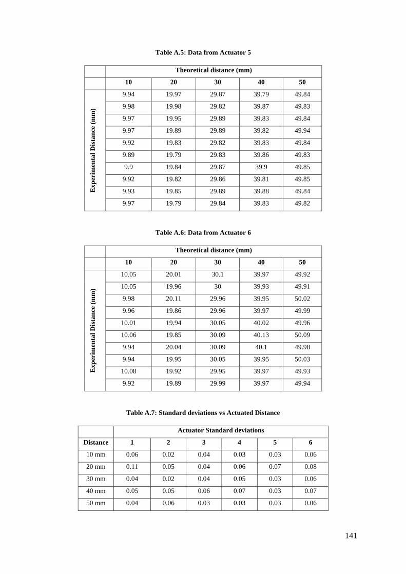
141
Table A.5: Data from Actuator 5
Theoretical distance (mm)
10 20 30 40 50
Ex
per
imen
tal
Dis
tan
ce (
mm
) 9.94 19.97 29.87 39.79 49.84
9.98 19.98 29.82 39.87 49.83
9.97 19.95 29.89 39.83 49.84
9.97 19.89 29.89 39.82 49.94
9.92 19.83 29.82 39.83 49.84
9.89 19.79 29.83 39.86 49.83
9.9 19.84 29.87 39.9 49.85
9.92 19.82 29.86 39.81 49.85
9.93 19.85 29.89 39.88 49.84
9.97 19.79 29.84 39.83 49.82
Table A.6: Data from Actuator 6
Theoretical distance (mm)
10 20 30 40 50
Ex
per
imen
tal
Dis
tan
ce (
mm
)
10.05 20.01 30.1 39.97 49.92
10.05 19.96 30 39.93 49.91
9.98 20.11 29.96 39.95 50.02
9.96 19.86 29.96 39.97 49.99
10.01 19.94 30.05 40.02 49.96
10.06 19.85 30.09 40.13 50.09
9.94 20.04 30.09 40.1 49.98
9.94 19.95 30.05 39.95 50.03
10.08 19.92 29.95 39.97 49.93
9.92 19.89 29.99 39.97 49.94
Table A.7: Standard deviations vs Actuated Distance
Actuator Standard deviations
Distance 1 2 3 4 5 6
10 mm 0.06 0.02 0.04 0.03 0.03 0.06
20 mm 0.11 0.05 0.04 0.06 0.07 0.08
30 mm 0.04 0.02 0.04 0.05 0.03 0.06
40 mm 0.05 0.05 0.06 0.07 0.03 0.07
50 mm 0.04 0.06 0.03 0.03 0.03 0.06

142
A.2 Inverse Kinematic Simulations – MATLAB® and SolidWorks®
Table A.8 to Table A.10 presents the data obtained from the inverse kinematic simulations conducted on
MATLAB® and SolidWorks® for verification of the inverse kinematic equations.
Table A.8: Testing of translation of the end effector
Region 1
End effector position (mm) Largest error among the six legs (mm)
x y z MATLAB Script Error Simulink Error
148.97 -114.54 278.54 0 0
147.59 -109.37 281.74 0.01 0.01
148.97 -99.44 282.38 0 0
160.14 -92.11 287.48 0.01 0.01
129.08 -84.62 300.76 0.01 0.01
130.69 -91.17 298.5 0 0
161.24 -86.62 270.51 0 0
134.32 -95.17 297.52 0.01 0.01
89.91 -132.26 303.31 0 0
87.57 -133.08 303.82 0 0
Region 2
End effector position (mm) Largest error among the six legs (mm)
x y z MATLAB Script Error Simulink Error
136.92 -70.03 308.22 0 0
113.35 -67.81 330.76 0 0
122.41 -56.32 331.43 0.01 0.01
128.65 -47.15 332.04 0.01 0.01
157.68 -28.35 304.34 0.01 0.01
159.16 -34.78 293.95 0.01 0.01
155.99 -39.59 292.26 0 0
158.61 -48.41 285.9 0.01 0.01
150.46 -55.85 287.61 0.01 0.01
146.94 -61.13 285.81 0 0
Region 3
End effector position (mm) Largest error among the six legs (mm)
x y z MATLAB Script Error Simulink Error
164.76 -21.49 298.54 0 0
170.05 -14.48 296.26 0 0
175.67 -6.54 294.69 0.01 0.01
169.44 -0.03 321.15 0 0
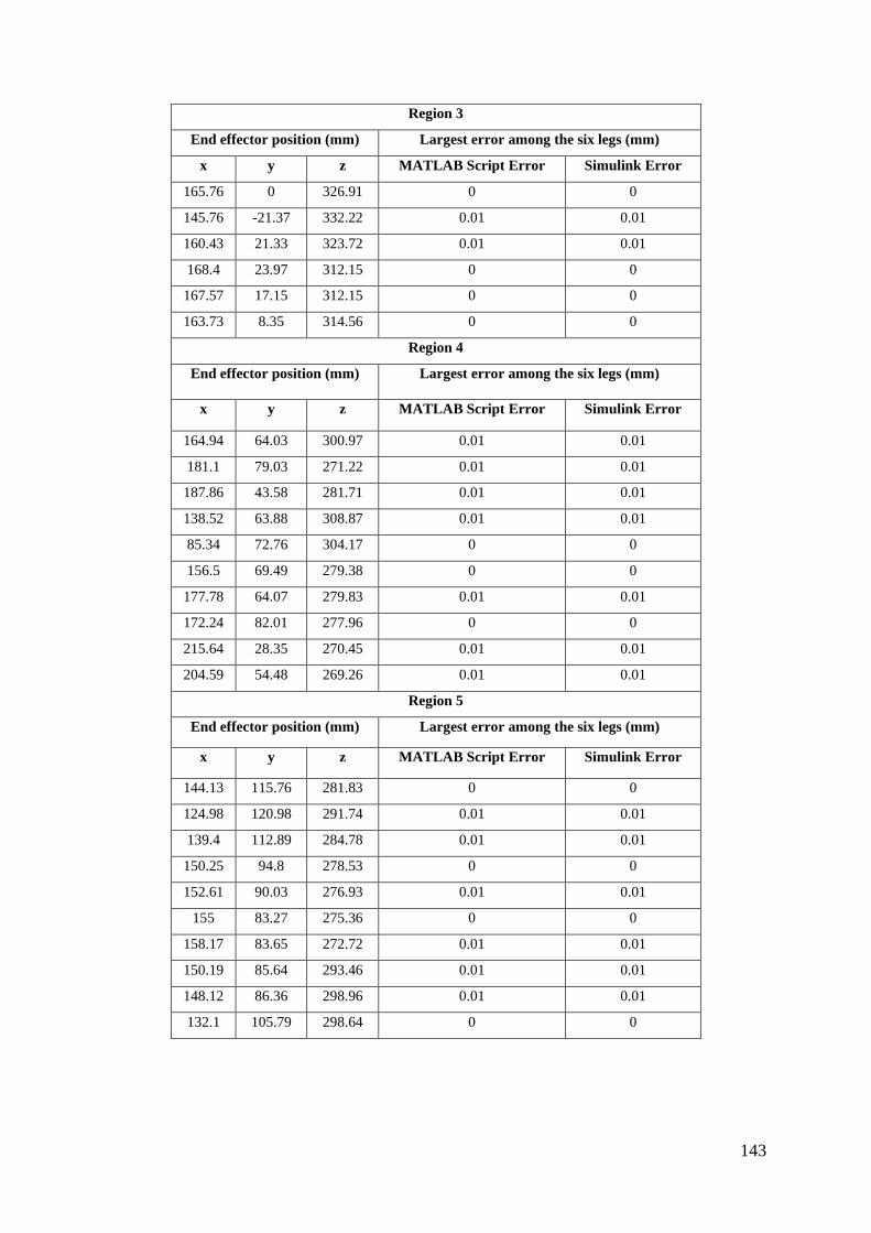
143
Region 3
End effector position (mm) Largest error among the six legs (mm)
x y z MATLAB Script Error Simulink Error
165.76 0 326.91 0 0
145.76 -21.37 332.22 0.01 0.01
160.43 21.33 323.72 0.01 0.01
168.4 23.97 312.15 0 0
167.57 17.15 312.15 0 0
163.73 8.35 314.56 0 0
Region 4
End effector position (mm) Largest error among the six legs (mm)
x y z MATLAB Script Error Simulink Error
164.94 64.03 300.97 0.01 0.01
181.1 79.03 271.22 0.01 0.01
187.86 43.58 281.71 0.01 0.01
138.52 63.88 308.87 0.01 0.01
85.34 72.76 304.17 0 0
156.5 69.49 279.38 0 0
177.78 64.07 279.83 0.01 0.01
172.24 82.01 277.96 0 0
215.64 28.35 270.45 0.01 0.01
204.59 54.48 269.26 0.01 0.01
Region 5
End effector position (mm) Largest error among the six legs (mm)
x y z MATLAB Script Error Simulink Error
144.13 115.76 281.83 0 0
124.98 120.98 291.74 0.01 0.01
139.4 112.89 284.78 0.01 0.01
150.25 94.8 278.53 0 0
152.61 90.03 276.93 0.01 0.01
155 83.27 275.36 0 0
158.17 83.65 272.72 0.01 0.01
150.19 85.64 293.46 0.01 0.01
148.12 86.36 298.96 0.01 0.01
132.1 105.79 298.64 0 0

144
Table A.9: Testing of translation and alpha rotation of the end effector
Region 1
End effector position and orientation Largest error among the six legs
(mm)
x (mm) y (mm) z (mm) alpha (deg) MATLAB
Script Error
Simulink Error
111.31 -95.52 312.28 17.6 0.01 0.01
111.31 -95.51 303.26 14.7 0 0
111.31 -124.39 281.2 -9.47 0 0
111.31 -127.91 276.8 -13.17 0.01 0.01
111.31 -136.1 274.14 -26.47 0 0
111.31 -132.5 287.35 -23.2 0 0
111.31 -137 288.2 -27.33 0.01 0.01
111.31 -83.2 310.18 14.24 0 0
111.31 -99.3 296.79 10.03 0 0
111.31 -103.58 291.69 4.59 0 0
Region 2
End effector position and orientation Largest error among the six legs
(mm)
x (mm) y (mm) z (mm) alpha (deg) MATLAB
Script Error
Simulink Error
111.31 -55.66 310.27 23.08 0 0
111.31 -48.88 311.43 20.09 0.01 0.01
111.31 -61.66 296.01 7.97 0 0
111.31 -72.34 292.99 5.7 0.01 0.01
111.31 -80.53 293.2 3.47 0 0
111.31 -77.71 297.02 -9.09 0.01 0.01
111.31 -53.11 306.11 -7.3 0.01 0.01
111.31 -51.18 316.62 -13.65 0.01 0.01
111.31 -38.81 326.94 -18.27 0 0
111.31 -41.52 319.78 -23.59 0 0
Region 3
End effector position and orientation Largest error among the six legs
(mm)
x (mm) y (mm) z (mm) alpha (deg) MATLAB
Script Error
Simulink Error
111.31 -5.05 318.5 -9.49 0.01 0.01

145
Region 3
End effector position and orientation Largest error among the six legs
(mm)
x (mm) y (mm) z (mm) alpha (deg) MATLAB
Script Error
Simulink Error
111.31 10.58 321.54 -14.49 0 0
111.31 19.38 315.73 -20.98 0 0
111.31 26.36 313.45 -14.33 0.01 0.01
111.31 14.3 317.72 -15.7 0.01 0.01
111.31 13.51 333.27 9.28 0 0
111.31 -25.87 316.7 12.21 0.01 0.01
111.31 -21.81 315.45 23.84 0.01 0.01
111.31 9.68 311.57 18.5 0 0
111.31 13.02 332.24 16.77 0 0
Region 4
End effector position and orientation Largest error among the six legs
(mm)
x (mm) y (mm) z (mm) alpha (deg) MATLAB
Script Error
Simulink Error
111.31 48.04 336.95 13.37 0 0
111.31 58.71 325.55 8.22 0.01 0.01
111.31 79.97 317.08 22.07 0 0
111.31 66 324.13 30.36 0.01 0.01
111.31 30.14 315.06 10.71 0 0
111.31 46.1 307.93 -18.5 0 0
111.31 32.78 310.15 -20.57 0 0
111.31 56.34 304.9 -15.87 0.01 0.01
111.31 67.52 302.91 -16.9 0.01 0.01
111.31 60.81 313.75 -22.7 0.01 0.01
Region 5
End effector position and orientation Largest error among the six legs
(mm)
x (mm) y (mm) z (mm) alpha (deg) MATLAB
Script Error
Simulink Error
111.31 85.08 298.26 -18.22 0.01 0.01
111.31 92.57 299.83 -22.23 0.01 0.01
111.31 96.44 288.07 -15.59 0.01 0.01
111.31 86.15 295.5 -20.99 0.01 0.01

146
Region 5
End effector position and orientation Largest error among the six legs
(mm)
x (mm) y (mm) z (mm) alpha (deg) MATLAB
Script Error
Simulink Error
111.31 96.42 282.39 -12.62 0 0
111.31 85.49 313.16 7.61 0 0
111.31 89.29 303.22 13.3 0 0
111.31 110.42 300.47 26.66 0 0
111.31 112.58 284.92 31.34 0 0
111.31 125.08 303.95 22.18 0.01 0.01
Table A.10: Testing of translation and beta rotation of the end effector
Region 1
End effector position and orientation Largest error among the six legs
(mm)
x (mm) y (mm) z (mm) beta (deg) MATLAB
Script Error
Simulink Error
169.32 -95.78 278.21 -6.96 0.01 0.01
177.57 -87.67 290.85 -16.06 0 0
167.71 -93.86 298.91 -17.24 0.01 0.01
173.24 -84.1 288.35 -8.88 0.01 0.01
174.74 -91.09 285.73 -6.77 0 0
114.75 -103.19 286.65 15.47 0 0
116.57 -106.44 284.7 18.56 0.01 0.01
114.77 -117.2 273.76 16.77 0 0
109.27 -124.83 275.92 19.13 0 0
129.67 -123.89 273.1 13.43 0 0
Region 2
End effector position and orientation Largest error among the six legs
(mm)
x (mm) y (mm) z (mm) beta (deg) MATLAB
Script Error
Simulink Error
136.69 -78.46 282.92 4.51 0 0
118.01 -69.31 315.82 3.9 0.01 0.01
105.04 -56.96 330.49 -9.24 0 0
87.63 -29.67 312.22 15.43 0 0

147
Region 2
End effector position and orientation Largest error among the six legs
(mm)
x (mm) y (mm) z (mm) beta (deg) MATLAB
Script Error
Simulink Error
89.05 -50 313.75 13.22 0.01 0.01
74.79 -32.86 320.49 -19.3 0 0
74.89 -28.15 333.17 -19.77 0 0
84.68 -51.78 329.98 -25.19 0 0
104.96 -32.74 324.21 18.37 0 0
111.7 -30.72 315.42 -14.41 0 0
Region 3
End effector position and orientation Largest error among the six legs
(mm)
x (mm) y (mm) z (mm) beta (deg) MATLAB
Script Error
Simulink Error
112.18 12.33 319.06 -13.86 0 0
111.96 27.29 329.44 -20.27 0 0
110.47 25.81 311.94 20.18 0.01 0.01
135.62 -26.63 310.7 15.46 0.01 0.01
137.68 -8.73 314.89 13.36 0.01 0.01
113.89 -14 325.31 -12.12 0.01 0.01
105.57 -7.03 329.67 -17.61 0 0
107.08 5.78 336.18 -20.7 0 0
96.55 11.29 315.62 10.95 0 0
85.11 27.12 317.28 12.36 0 0
Region 4
End effector position and orientation Largest error among the six legs
(mm)
x (mm) y (mm) z (mm) beta (deg) MATLAB
Script Error
Simulink Error
82.25 50.87 316.73 15.62 0.01 0.01
115.72 55.22 302.85 19.29 0 0
87.87 31.1 327.35 -17.77 0 0
123.93 34.77 324.32 -6.33 0.01 0.01
131.36 30.24 320.84 -2.81 0 0
129.8 70.98 322.11 2.62 0.01 0.01
131.49 81.71 323.51 2.63 0 0

148
Region 4
End effector position and orientation Largest error among the six legs
(mm)
x (mm) y (mm) z (mm) beta (deg) MATLAB
Script Error
Simulink Error
128.28 49.13 308.65 -13.66 0 0
115.95 28.64 307.89 -19.38 0 0
118.43 25.69 318.92 19.52 0 0
Region 5
End effector position and orientation Largest error among the six legs
(mm)
x (mm) y (mm) z (mm) beta (deg) MATLAB
Script Error
Simulink Error
138.66 90.27 301.95 0.34 0 0
141.28 93.12 305.74 -7.95 0.01 0.01
117.85 115.26 299.62 -5.68 0 0
103.53 109.48 298.23 10.43 0.01 0.01
86.07 112.07 310.08 -3.98 0.01 0.01
89.97 83.43 317.48 15.41 0.01 0.01
144.81 91.86 297.63 2.08 0 0
143 109.68 304.28 -12.74 0 0
142.16 82.55 302.64 -13.86 0.01 0.01
106.86 83.55 314.62 13.14 0 0
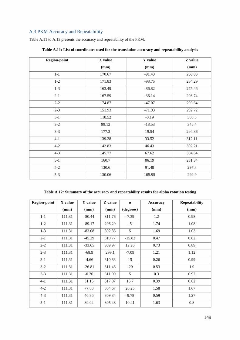
149
A.3 PKM Accuracy and Repeatability
Table A.11 to A.13 presents the accuracy and repeatability of the PKM.
Table A.11: List of coordinates used for the translation accuracy and repeatability analysis
Region-point X value
(mm)
Y value
(mm)
Z value
(mm)
1-1 170.67 -91.43 268.83
1-2 171.83 -98.75 264.29
1-3 163.49 -86.82 275.46
2-1 167.59 -36.14 293.74
2-2 174.87 -47.07 293.64
2-3 151.93 -71.93 292.72
3-1 110.52 -0.19 305.5
3-2 99.12 -18.53 345.4
3-3 177.3 19.54 294.36
4-1 139.28 33.52 312.11
4-2 142.83 46.43 302.21
4-3 145.77 67.62 304.64
5-1 160.7 86.19 281.34
5-2 130.6 91.48 297.3
5-3 130.06 105.95 292.9
Table A.12: Summary of the accuracy and repeatability results for alpha rotation testing
Region-point X value
(mm)
Y value
(mm)
Z value
(mm)
α
(degrees)
Accuracy
(mm)
Repeatability
(mm)
1-1 111.31 -80.44 311.76 -7.39 1.2 0.98
1-2 111.31 -89.17 296.29 -5 1.74 1.08
1-3 111.31 -83.08 302.83 5 1.69 1.03
2-1 111.31 -45.29 310.77 -15.82 0.47 0.82
2-2 111.31 -33.65 309.97 12.26 0.73 0.89
2-3 111.31 -68.9 299.1 -7.09 1.21 1.12
3-1 111.31 -4.66 310.83 15 0.26 0.99
3-2 111.31 -26.81 311.43 -20 0.53 1.9
3-3 111.31 -0.26 311.09 5 0.3 0.92
4-1 111.31 31.15 317.07 16.7 0.39 0.62
4-2 111.31 77.88 304.67 20.25 1.58 1.67
4-3 111.31 46.86 309.34 -9.78 0.59 1.27
5-1 111.31 89.04 305.48 10.41 1.63 0.8

150
Region-point X value
(mm)
Y value
(mm)
Z value
(mm)
α
(degrees)
Accuracy
(mm)
Repeatability
(mm)
5-2 111.31 103.97 299.41 8.78 1.63 0.78
5-3 111.31 84.59 306.17 -2.3 1.25 0.23
Table A.13: Summary of the accuracy and repeatability results for beta rotation testing
Region-point X value
(mm)
Y value
(mm)
Z value
(mm)
β
(degrees)
Accuracy
(mm)
Repeatability
(mm)
1-1 124.47 -90.11 287.16 10.11 1.55 0.79
1-2 101.57 -97.88 314.82 -5.52 1.76 0.73
1-3 105.16 -93.48 322.4 -12.64 1.73 0.86
2-1 105.45 -33.76 317.56 8.57 1.37 0.47
2-2 113.84 -31.64 308.17 15.11 0.7 1.34
2-3 97.84 -54.65 322.13 -9.43 1.34 0.63
3-1 164.34 -15 305.66 -11.02 0.21 0.58
3-2 164.48 15.15 296.16 -17.46 0.3 1.07
3-3 138.51 23.44 304.56 9.33 0.45 0.96
4-1 111.03 43.04 308.45 12.93 0.7 1.04
4-2 135.94 29.14 319.64 -12.48 0.62 0.64
4-3 137.56 51.8 315.32 -4 0.66 0.28
5-1 123.69 91.82 287.49 11.87 1.54 0.94
5-2 151.61 95.94 273.93 6.89 1.46 0.47
5-3 142.28 84.02 301.35 -7.8 1.69 0.5

151
A.4 Payload Tests
Table A.14 presents the data for the load vs. leg actuation error investigation.
Table A.14: Load vs. Leg Actuation Error
Error (mm)
Load (kg) Leg 1 Leg 2 Leg 3 Leg 4 Leg 5 Leg 6
0.45 0.11 0.07 0.08 0.06 0.03 0.06
1 0.03 0.02 0.09 0.08 0.08 0.05
1.45 0.05 0.06 0.05 0.03 0.06 0.11
2 0.13 0.06 0.05 0.05 0.03 0.12
2.45 0.01 0.03 0.02 0.04 0.09 0.01
3 0.03 0.16 0.02 0.17 0.16 0.14
3.45 0.1 0.03 0.19 0.22 0.03 0.09
5.27 0.03 0.09 0.05 0.02 0.19 0.18
6.18 0.02 0.03 0.13 0.05 0.09 0.17
7.08 0.21 0.29 0.27 0.09 0.16 0.14
8.44 0.03 0.24 0.26 0.02 0.2 0.08
9.35 0.19 0.26 0.17 0.27 0.03 0
10.26 0.06 0.09 0.08 0.03 0.09 0.07
12.07 0.07 0.25 0.21 0.28 0.03 0.09
13.43 0.06 0.05 0.02 0.07 0.11 0.01
15 0.21 0.04 0.22 0.14 0.05 0.05
18 0.06 0.05 0.12 0.08 0.04 0.01
20 0.1 0.04 0.05 0.02 0 0.02
23 0.02 0.03 0.04 0.01 0.04 0.08
25.23 0.02 0.09 0.06 0.11 0.14 0.13

152
A.5 Forward Kinematic Simulations – MATLAB® and SolidWorks®
Table A.15 to Table A.17 displays the results obtained from the simulations of the forward kinematic analysis
performed with MATLAB® and SolidWorks®.
Table A.15: Forward kinematic results for translation
Region 1 mm degrees
x y z 𝜽𝟏 𝜽𝟑 𝜽𝟓
True value 126.98 -120.41 290.84 64.33 42.82 122.78
Guess 150 -150 350 57.3 57.3 108.86
Converged value 126.98 -120.4 290.84 64.33 42.82 122.87
Absolute error 0 0.01 0 0 0 0.09
Iterations 5
True value 99.96 -113.57 311.91 74.44 50 118.7
Guess 150 -70 350 51.57 40.11 108.86
Converged value 99.96 -113.57 311.9 74.43 50 118.73
Absolute error 0 0 0.01 0.01 0 0.03
Iterations 5
True value 149.04 -87.7 280.25 57.12 42.27 115.77
Guess 220 -10 220 63.03 34.38 103.13
Converged value 149.05 -87.69 280.25 57.11 42.27 116.17
Absolute error 0.01 0.01 0 0.01 0 0.4
Iterations 7
True value 155.94 -100.29 274.59 54.39 39.05 119.25
Guess 100 -70 350 68.75 45.84 120.32
Converged value 155.94 -100.3 274.6 54.39 39.05 119.93
Absolute error 0 0.01 0.01 0 0 0.68
Iterations 5
True value 146.93 -104.65 288.73 59.03 42.15 118.92
Guess 0 0 0 0 0 0
Converged value 146.92 -104.66 288.72 59.03 42.15 119.3
Absolute error 0.01 0.01 0.01 0 0 0.38
Iterations 6
Region 2 mm degrees
x y z 𝜽𝟏 𝜽𝟑 𝜽𝟓
True value 145.09 -77.8 293.73 60.08 46.29 111.91

153
Region 2 mm degrees
x y z 𝜽𝟏 𝜽𝟑 𝜽𝟓
Guess 100 -20 150 45.84 57.3 126.05
Converged value 145.08 -77.8 293.74 60.08 46.29 112.15
Absolute error 0.01 0 0.01 0 0 0.24
Iterations 6
True value 133.25 -68.42 320.35 66.12 53.19 107.49
Guess 180 -20 380 44.12 36.1 114.59
Converged value 133.24 -68.42 320.35 66.13 53.19 107.56
Absolute error 0.01 0 0 0.01 0 0.07
Iterations 5
True value 137.97 -44.46 315.41 63.25 54.68 101.79
Guess 80 0 260 45.84 57.3 114.59
Converged value 137.95 -44.46 315.42 63.25 54.68 101.85
Absolute error 0.02 0 0.01 0 0 0.06
Iterations 6
True value 138.09 -33.61 315.04 62.44 55.87 98.98
Guess 200 20 354 50.42 35.52 54.43
Converged value 138.08 -33.61 315.03 62.45 55.87 99.03
Absolute error 0.01 0 0.01 0.01 0 0.05
Iterations 6
True value 116.55 -28.84 343.58 69.78 63.61 96.89
Guess 200 -50 400 57.3 68.75 111.73
Converged value 116.54 -28.84 343.59 69.79 63.62 96.89
Absolute error 0.01 0 0.01 0.01 0.01 0
Iterations 7
Region 3 mm degrees
x y z 𝜽𝟏 𝜽𝟑 𝜽𝟓
True value 119.65 -13.31 346.52 68 65.21 93.15
Guess 19 -50 400 74.48 57.3 106.57
Converged value 119.65 -13.32 346.51 68 65.21 93.16
Absolute error 0 0.01 0.01 0 0 0.01
Iterations 6
True value 115.85 3.48 342.62 66.64 67.41 89.16

154
Region 3 mm degrees
x y z 𝜽𝟏 𝜽𝟑 𝜽𝟓
Guess 30 80 400 74.48 74.48 101.99
Converged value 115.85 3.48 342.62 66.65 67.4 89.16
Absolute error 0 0 0 0.01 0.01 0
Iterations 6
True value 116.39 13.59 341.55 65.28 68.24 86.71
Guess 74 87 450 51.57 50.42 102.56
Converged value 116.4 13.6 341.54 65.29 68.23 86.65
Absolute error 0.01 0.01 0.01 0.01 0.01 0.06
Iterations 6
True value 186.11 0 312.8 50.32 50.32 90
Guess 220 42 366 57.3 63.03 74.48
Converged value 186.1 0 312.81 50.33 50.33 90
Absolute error 0.01 0 0.01 0.01 0.01 0
Iterations 5
True value 181.31 24.99 307.68 48.48 51.95 83.54
Guess 142 78 400 57.3 44.12 94.54
Converged value 181.3 24.99 307.68 48.48 51.95 83.29
Absolute error 0.01 0 0 0 0 0.25
Iterations 5
Region 4 mm degrees
x y z 𝜽𝟏 𝜽𝟑 𝜽𝟓
True value 172.03 64.7 295.64 44.37 53.69 72.52
Guess 115 96 333 35.52 37.24 80.21
Converged value 172.02 64.69 295.64 44.38 53.69 71.93
Absolute error 0.01 0.01 0 0.01 0 0.59
Iterations 5
True value 153.5 73.67 304.68 47.43 59.49 70.38
Guess 90 133 450 54.43 50.42 82.51
Converged value 153.5 73.68 304.68 47.42 59.49 70.08
Absolute error 0 0.01 0 0.01 0 0.3
Iterations 6
True value 103.86 69.1 333.17 58.94 74.6 73.17

155
Region 4 mm degrees
x y z 𝜽𝟏 𝜽𝟑 𝜽𝟓
Guess 33 155 488 42.97 63.03 49.27
Converged value 103.84 69.08 333.18 58.95 74.6 73.16
Absolute error 0.02 0.02 0.01 0.01 0 0.01
Iterations 6
True value 93.15 81.96 332.6 58.39 77.77 70.29
Guess 201 33 469 50.99 65.32 89.38
Converged value 93.15 81.98 332.6 58.38 77.77 70.24
Absolute error 0 0.02 0 0.01 0 0.05
Iterations 8
True value 91.6 32.76 351.24 68.01 76.12 82.46
Guess 244 -10 462 34.38 45.84 91.67
Converged value 91.61 32.77 351.24 68 76.11 82.44
Absolute error 0.01 0.01 0 0.01 0.01 0.02
Iterations 6
Region 5 mm degrees
x y z 𝜽𝟏 𝜽𝟑 𝜽𝟓
True value 88.58 86.16 332.63 58.32 79.07 69.42
Guess 256 10 488 31.51 55.58 46.98
Converged value 88.57 86.16 332.64 58.32 79.07 69.35
Absolute error 0.01 0 0.01 0 0 0.07
Iterations 7
True value 111.71 109.13 297.75 47.1 69.86 60.48
Guess 280 222 350 34.38 45.84 44.12
Converged value 111.71 109.13 297.75 47.1 69.86 60.48
Absolute error 0 0 0 0 0 0
Iterations 7
True value 140.21 116.77 284.1 40.7 59.85 57.47
Guess 193 88 201 37.82 44.69 74.48
Converged value 140.21 116.77 284.1 40.7 59.85 57.16
Absolute error 0 0 0 0 0 0.31
Iterations 6
True value 156.25 86.16 285.71 42.53 56.18 65.55

156
Region 5 mm degrees
x y z 𝜽𝟏 𝜽𝟑 𝜽𝟓
Guess 220 30 350 0 28.65 28.65
Converged value 156.25 86.16 285.7 42.53 56.18 65.04
Absolute error 0 0 0.01 0 0 0.51
Iterations 6
True value 80.56 135.59 305.19 47.6 78.32 56.44
Guess 120 100 450 37.82 63.03 74.48
Converged value 80.55 135.59 305.19 47.6 78.32 56.14
Absolute error 0.01 0 0 0 0 0.3
Iterations 6
Table A.16: Forward kinematic results for alpha rotation and translation
Region 1 mm degrees
x y z α 𝜽𝟏 𝜽𝟑 𝜽𝟓
True value 111.31 -126.79 297.78 -12.41 69.51 41.02 122.91
Guess 150 -100 350 -17.19 80.21 57.3 108.29
Converged value 111.29 -126.78 297.79 -12.4 69.52 41.02 122.91
Absolute error 0.02 0.01 0.01 0.01 0.01 0 0
Iterations 5
True value 111.31 -109.59 303.08 6.78 70.27 49.79 118.86
Guess 80 -50 289 11.46 80.21 37.82 120.32
Converged value 111.32 -109.6 303.07 6.78 70.26 49.79 118.87
Absolute error 0.01 0.01 0.01 0 0.01 0 0.01
Iterations 5
True value 111.31 -85.7 331.42 -10.8 73.71 52.55 110.84
Guess 145 -10 300 14.32 57.3 57.3 85.94
Converged value 111.31 -85.7 331.43 -10.81 73.71 52.55 110.84
Absolute error 0 0 0.01 0.01 0 0 0
Iterations 6
True value 111.31 -96.78 297.23 12.21 69.27 52.08 116.31
Guess 95 -133 220 18.91 57.3 45.84 74.48
Converged value 111.33 -96.79 297.22 12.22 69.26 52.08 116.32
Absolute error 0.02 0.01 0.01 0.01 0.01 0 0.01

157
Region 1 mm degrees
x y z α 𝜽𝟏 𝜽𝟑 𝜽𝟓
Iterations 6
True value 111.31 -121.99 296.16 -21 69.88 38.61 121.61
Guess 100 -60 350 -22.92 74.48 45.84 126.05
Converged value 111.3 -122 296.17 -21 69.97 38.63 121.6
Absolute error 0.01 0.01 0.01 0 0.09 0.02 0.01
Iterations 6
Region 2 mm degrees
x y z α 𝜽𝟏 𝜽𝟑 𝜽𝟓
True value 111.31 -76.73 296.83 -16.95 71.23 46.35 111.74
Guess 120 -60 300 -28.65 85.94 68.75 85.94
Converged value 111.32 -76.73 296.82 -16.95 71.22 46.34 111.74
Absolute error 0.01 0 0.01 0 0.01 0.01 0
Iterations 6
True value 111.31 -37.14 323.67 -26.69 73.06 53.91 100.19
Guess 80 -80 300 -28.65 80.21 63.03 85.94
Converged value 111.3 -37.1 323.67 -26.68 73.05 53.91 100.19
Absolute error 0.01 0.04 0 0.01 0.01 0 0
Iterations 5
True value 111.31 -28.61 316.81 23.87 63.85 66.03 94.66
Guess 100 0 300 28.65 51.57 51.57 74.48
Converged value 111.3 -28.59 316.81 23.88 63.85 66.03 94.65
Absolute error 0.02 0.02 0 0.01 0 0 0.01
Iterations 5
True value 111.31 -67.4 304.31 9.53 69 56.61 108.11
Guess 99 -30 390 12.61 45.84 57.3 101.99
Converged value 111.32 -67.43 304.3 9.51 69 56.6 108.12
Absolute error 0.01 0.03 0.01 0.02 0 0.01 0.01
Iterations 5
True value 111.31 -41.35 326.51 20.74 67.32 64.93 98.39
Guess 10 -20 365 5.73 57.3 57.3 95.11
Converged value 111.33 -41.37 326.5 20.74 67.32 64.92 98.39
Absolute error 0.02 0.02 0.01 0 0 0.01 0

158
Region 2 mm degrees
x y z α 𝜽𝟏 𝜽𝟑 𝜽𝟓
Iterations 6
Region 3 mm degrees
x y z α 𝜽𝟏 𝜽𝟑 𝜽𝟓
True value 111.31 0.69 320.1 14.32 62.47 68.18 87.92
Guess 48 50 330 5.73 51.57 45.84 91.67
Converged value 111.28 0.73 320.1 14.33 62.48 68.19 87.9
Absolute error 0.03 0.04 0 0.01 0.01 0.01 0.02
Iterations 5
True value 111.31 -26.92 332.84 -20.87 72.44 58.59 97.56
Guess 62 10 341 22.92 74.48 68.75 108.86
Converged value 111.29 -26.92 332.85 -20.86 72.44 58.59 97.56
Absolute error 0.02 0 0.01 0.01 0 0 0
Iterations 6
True value 111.31 19.34 329.02 -27.56 68.71 63.19 86.85
Guess 12 61 280 -34.38 74.48 68.75 103.13
Converged value 111.32 19.36 329.02 -27.57 68.71 63.19 86.85
Absolute error 0.01 0.02 0 0.01 0 0 0
Iterations 7
True value 111.31 -11.39 314.44 13.97 63.5 66.21 91.37
Guess 30 -60 320 17.19 74.48 77.92 92.82
Converged value 111.33 -11.41 314.44 13.97 63.5 66.22 91.41
Absolute error 0.02 0.02 0 0 0 0.01 0.04
Iterations 6
True value 111.31 16.67 322.14 29.02 56.17 71.79 80.77
Guess 80 30 300 34.38 57.3 57.3 74.48
Converged value 111.3 16.68 322.14 29.03 56.17 71.8 80.76
Absolute error 0.01 0.01 0 0.01 0 0.01 0.01
Iterations 5
Region 4 mm degrees
x y z α 𝜽𝟏 𝜽𝟑 𝜽𝟓
True value 111.31 72.62 293.73 9.23 48.93 70.13 67.2
Guess 60 60 233 13.18 56.72 45.84 51.57
Converged value 111.32 72.61 293.72 9.23 48.93 70.12 67.2

159
Region 4 mm degrees
x y z α 𝜽𝟏 𝜽𝟑 𝜽𝟓
Absolute error 0.01 0.01 0.01 0 0 0.01 0
Iterations 6
True value 111.31 79.99 307.43 13.71 48.79 71.95 65.93
Guess 31 2 300 17.19 51.57 57.3 45.84
Converged value 111.32 79.98 307.43 13.71 48.8 71.95 65.94
Absolute error 0.01 0.01 0 0 0.01 0 0.01
Iterations 6
True value 111.31 29.97 314.49 8.16 59.03 69.56 80.66
Guess 10 66 358 5.16 68.75 57.3 65.89
Converged value 111.3 29.97 314.49 8.16 59.03 69.56 80.66
Absolute error 0.01 0 0 0 0 0 0
Iterations 6
True value 111.31 30.11 317.09 -14.77 64.34 66.06 83.43
Guess 10 90 285 -22.92 74.48 80.21 108.86
Converged value 111.31 30.13 317.08 -14.77 64.34 66.06 83.42
Absolute error 0 0.02 0.01 0 0 0 0.01
Iterations 7
True value 111.31 69.59 320.08 -25.99 61.53 68.75 74.81
Guess 55 20 289 -34.38 68.75 68.75 85.94
Converged value 111.3 69.63 320.07 -25.98 61.52 68.74 74.8
Absolute error 0.01 0.04 0.01 0.01 0.01 0.01 0.01
Iterations 6
Region 5 mm degrees
x y z α 𝜽𝟏 𝜽𝟑 𝜽𝟓
True value 111.31 122.76 303.03 10.49 43.06 70.27 56.29
Guess 20 60 260 14.9 57.3 57.3 57.3
Converged value 111.3 122.76 303.03 10.49 43.06 70.27 56.29
Absolute error 0.01 0 0 0 0 0 0
Iterations 6
True value 111.31 104.07 286.88 26.66 37.2 70.33 54.55
Guess 150 120 222 32.09 42.4 85.94 40.11
Converged value 111.3 104.08 286.87 26.67 37.19 70.34 54.55

160
Region 5 mm degrees
x y z α 𝜽𝟏 𝜽𝟑 𝜽𝟓
Absolute error 0.01 0.01 0.01 0.01 0.01 0.01 0
Iterations 5
True value 111.31 64.05 296.11 10.35 50.3 70.21 69.54
Guess 160 50 320 17.19 68.75 80.21 57.3
Converged value 111.31 64.05 296.11 10.35 50.31 70.21 69.55
Absolute error 0 0 0 0 0.01 0 0.01
Iterations 5
True value 111.31 90.24 290.95 -7.7 50.87 68.72 65.42
Guess 148 78 369 -11.46 57.3 74.48 80.21
Converged value 111.31 90.23 290.96 -7.7 50.87 68.72 65.43
Absolute error 0 0.01 0.01 0 0 0 0.01
Iterations 6
True value 111.31 97.23 289.98 -17.08 52.13 68.05 64.95
Guess 85 60 350 -18.33 68.75 74.48 80.21
Converged value 111.31 97.24 290 -17.09 52.13 68.04 64.95
Absolute error 0 0.01 0.02 0.01 0 0.01 0
Iterations 6
Table A.17: Forward kinematic results for beta rotation and translation
Region 1 mm degrees
x y z β 𝜽𝟏 𝜽𝟑 𝜽𝟓
True value 133.68 -99.6 280.91 15.38 66.26 46.4 120.69
Guess 180 -55 354 5.73 5.61 35.52 105.42
Converged value 133.67 -99.6 280.91 15.38 66.26 46.4 120.86
Absolute error 0.02 0 0 0 0 0 0.17
Iterations 7
True value 164.5 -85.91 282.78 12.68 57.78 44.08 115.28
Guess 200 -40 230 5.73 50.42 51.57 97.4
Converged value 164.46 -85.92 282.79 12.69 57.79 44.09 116.08
Absolute error 0.04 0.01 0.01 0.01 0.01 0.01 0.8
Iterations 6

161
Region 1 mm degrees
x y z β 𝜽𝟏 𝜽𝟑 𝜽𝟓
True value 177.17 -94.51 280.85 -6.44 48.22 36.84 115.37
Guess 230 -10 360 11.46 51.57 25.78 95.11
Converged value 177.16 -94.5 280.86 -6.44 48.23 36.85 116.5
Absolute error 0.01 0.01 0.01 0 0.01 0.01 1.13
Iterations 6
True value 141.4 -104.53 308.05 -9.91 59.83 43.79 116.12
Guess 100 -70 369 -5.73 44.69 25.78 127.2
Converged value 141.38 -104.54 308.05 -9.91 59.83 43.8 116.31
Absolute error 0.02 0.01 0 0 0 0.01 0.19
Iterations 5
True value 140.14 -113.51 316.79 -15.87 59.15 43.08 116.75
Guess 200 -70 250 8.59 45.84 37.82 89.95
Converged value 140.12 -113.51 316.79 -15.87 59.15 43.08 116.89
Absolute error 0.02 0 0 0 0 0 0.14
Iterations 6
Region 2 mm degrees
x y z β 𝜽𝟏 𝜽𝟑 𝜽𝟓
True value 159.84 -58.84 304.91 -15.24 52.48 44.18 105.08
Guess 220 -12 400 8.59 48.13 34.38 31.51
Converged value 159.81 -58.85 304.92 -15.22 52.49 44.19 105.35
Absolute error 0.03 0.01 0.01 0.02 0.01 0.01 0.27
Iterations 5
True value 147.3 -55.31 327.04 -16.5 58.02 49.56 103.13
Guess 200 0 350 45.84 35.52 88.81 88.81
Converged value 147.32 -55.3 327.02 -16.51 58.01 49.56 103.24
Absolute error 0.02 0.01 0.02 0.01 0.01 0 0.11
Iterations 8
True value 128.17 -71.14 307.24 -8.02 63.38 49.69 108.83
Guess 200 -10 399 -22.92 51.57 57.3 114.59
Converged value 128.16 -71.15 307.24 -8.02 63.39 49.69 108.86
Absolute error 0.01 0.01 0 0 0.01 0 0.03
Iterations 6

162
Region 2 mm degrees
x y z β 𝜽𝟏 𝜽𝟑 𝜽𝟓
True value 149.18 -31.59 317.32 6.91 62.02 56.22 98.44
Guess 180 -60 350 8.02 68.75 68.75 91.67
Converged value 149.17 -31.6 317.32 6.92 62.02 56.22 98.54
Absolute error 0.01 0.01 0 0.01 0 0 0.1
Iterations 7
True value 147.35 -28.99 316.28 7.99 62.37 56.93 97.84
Guess 150 -10 320 5.73 51.57 45.84 91.67
Converged value 147.34 -29 316.28 7.99 62.38 56.92 97.92
Absolute error 0.01 0.01 0 0 0.01 0.01 0.08
Iterations 5
Region 3 mm degrees
x y z β 𝜽𝟏 𝜽𝟑 𝜽𝟓
True value 152.56 -4.41 297.08 -8.14 51.86 51.1 91.24
Guess 100 -50 200 -17.19 71.62 74.48 70.47
Converged value 152.56 -4.39 297.07 -8.14 51.86 51.1 91.25
Absolute error 0 0.02 0.01 0 0 0 0.01
Iterations 7
True value 161.27 0.78 297.98 -19.62 46.21 46.32 89.79
Guess 82 36 369 25.78 34.38 31.51 75.63
Converged value 161.27 0.77 297.97 -19.64 46.21 46.32 89.79
Absolute error 0 0.01 0.01 0.02 0 0 0
Iterations 6
True value 167.33 16.03 311.93 -24.02 45.24 47.26 86.05
Guess 0 50 295 -28.65 34.38 40.11 72.19
Converged value 167.35 16.04 311.91 -24.04 45.24 47.26 85.94
Absolute error 0.02 0.01 0.02 0.02 0 0 0.11
Iterations 6
True value 119.78 25.1 305.46 11.34 61.7 67.81 82.59
Guess 150 0 260 11.46 51.57 51.57 74.48
Converged value 119.85 25.09 305.44 11.31 61.68 67.79 82.59
Absolute error 0.07 0.01 0.02 0.03 0.02 0.02 0
Iterations 5

163
Region 3 mm degrees
x y z β 𝜽𝟏 𝜽𝟑 𝜽𝟓
True value 117.27 26.1 312 19.41 64.45 70.75 82.35
Guess 185 -10 280 22.92 57.3 57.3 68.75
Converged value 117.28 26.07 312 19.41 64.45 70.75 82.35
Absolute error 0.01 0.03 0 0 0 0 0
Iterations 6
Region 4 mm degrees
x y z β 𝜽𝟏 𝜽𝟑 𝜽𝟓
True value 159.9 50.99 296.7 3.96 48.66 57.25 75.59
Guess 120 6 312 5.73 57.3 68.75 88.81
Converged value 159.87 50.99 296.72 3.98 48.67 57.26 75.28
Absolute error 0.03 0 0.02 0.02 0.01 0.01 0.31
Iterations 5
True value 145.35 60.79 293.44 6.45 49.83 61.44 72.15
Guess 100 100 350 18.91 57.3 71.62 82.51
Converged value 145.38 60.78 293.43 6.44 49.82 61.43 71.96
Absolute error 0.03 0.01 0.01 0.01 0.01 0.01 0.19
Iterations 5
True value 120.8 68.1 319.23 -12.08 52 65.29 72.99
Guess 196 30 387 -20.05 63.03 48.7 77.92
Converged value 120.83 68.1 319.22 -12.09 52 65.28 72.98
Absolute error 0.03 0 0.01 0.01 0 0.01 0.01
Iterations 5
True value 125.83 73.89 329.36 -21.08 49.88 62.34 72.8
Guess 80 130 355 -34.38 68.75 63.03 76.2
Converged value 125.82 73.9 329.35 -21.08 49.88 62.34 72.79
Absolute error 0.01 0.01 0.01 0 0 0 0.01
Iterations 5
True value 115.02 51.64 323.2 -7.95 56.62 67.73 77
Guess 35 20 266 -28.65 63.03 74.48 85.94
Converged value 114.99 51.66 323.21 -7.94 56.63 67.74 76.99
Absolute error 0.03 0.02 0.01 0.01 0.01 0.01 0.01
Iterations 6

164
Region 5 mm degrees
x y z β 𝜽𝟏 𝜽𝟑 𝜽𝟓
True value 100.93 94.37 294.47 3.87 50.83 74.09 63.26
Guess 22 49 320 6.3 57.3 57.3 45.84
Converged value 100.92 94.38 294.47 3.87 50.83 74.09 63.23
Absolute error 0.01 0.01 0 0 0 0 0.03
Iterations 5
True value 101.02 103.8 314.55 -4.79 50.73 73.14 64.04
Guess 166 150 277 2.86 68.75 80.21 50.42
Converged value 101.06 103.78 314.54 -4.81 50.73 73.13 64.02
Absolute error 0.04 0.02 0.01 0.02 0 0.01 0.02
Iterations 5
True value 81.94 121.76 308.99 -5.86 49.09 77.4 60.08
Guess 174 66 266 -20.63 68.75 85.94 42.4
Converged value 81.95 121.77 308.99 -5.87 49.09 77.4 59.85
Absolute error 0.01 0.01 0 0.01 0 0 0.23
Iterations 6
True value 105.77 113.46 282.27 10.39 46.69 73.01 56.36
Guess 221 80 250 0 57.3 57.3 44.12
Converged value 105.75 113.47 282.27 10.4 46.69 73.02 56.34
Absolute error 0.02 0.01 0 0.01 0 0.01 0.02
Iterations 7
True value 125.16 118.16 299.55 -4.15 43.88 64.64 59.19
Guess 130 90 350 -51.57 51.57 57.3 45.84
Converged value 125.15 118.17 299.55 -4.15 43.88 64.64 59.13
Absolute error 0.01 0.01 0 0 0 0 0.06
Iterations 8

165
A.6 Forward Kinematic Simulations – Guess Deviations Analysis
Table A.18 to Table A.23 presents the data obtained from the guess deviation analysis and was used to generate
the graphs shown in Section 8.9.
Table A.18: Guess deviations and number of iterations for x, y and z values for translation
Guess deviation
(mm)
Number of iterations
x y z
-250 8 8 Incorrect convergence
-200 7 7 Diverges
-150 6 6 Incorrect convergence
-100 5 5 6
-50 5 5 5
50 5 5 5
100 6 6 5
150 7 6 6
200 8 8 6
250 Incorrect convergence Diverges 7
Table A.19: Guess deviations and number of iterations for θ1, θ3 and θ5 values for translation
Guess deviation
(degrees)
Number of iterations
θ1 θ3 θ5
-100 9 8 Diverges
-80 8 8 14
-60 6 6 6
-40 6 5 5
-20 5 5 5
20 5 5 5
40 Diverges Diverges 6
60 10 Diverges Incorrect convergence
80 Diverges Diverges Diverges
100 Diverges 13 Incorrect convergence

166
Table A.20: Guess deviations and number of iterations for x, y and z values for α rotation and translation
Guess deviation
(mm)
Number of iterations
x y z
-100 6 7 Diverges
-80 6 6 7
-60 5 6 6
-40 5 5 5
-20 4 4 4
20 4 4 4
40 5 5 5
60 6 5 5
80 7 6 6
100 Diverges 6 6
Table A.21: Guess deviations and number of iterations for α, θ1, θ3 and θ5 values for α rotation and
translation
Guess deviation
(degrees)
Number of iterations
α θ1 θ3 θ5
-100 9 Incorrect
convergence
Diverges Diverges
-80 8 7 8 Incorrect
convergence
-60 6 6 6 8
-40 5 6 6 6
-20 5 5 5 5
20 5 6 4 5
40 6 6 5 4
60 9 Diverges 7 6
80 Incorrect
convergence
Incorrect
convergence
Incorrect
convergence
Incorrect
convergence
100 Incorrect
convergence
Incorrect
convergence
Diverges Incorrect
convergence

167
Table A.22: Guess deviations and number of iterations for x, y and z values for β rotation and translation
Guess deviation
(mm)
Number of iterations
x y z
-250 Incorrect convergence Incorrect convergence Diverges
-200 7 8 Incorrect convergence
-150 6 6 7
-100 5 5 6
-50 5 5 5
50 5 5 5
100 5 5 5
150 6 6 6
200 8 8 6
250 Diverges Incorrect convergence 7
Table A.23: Guess deviations and number of iterations for β, θ1, θ3 and θ5 values for β rotation and
translation
Guess deviation
(degrees)
Number of iterations
β θ1 and θ3 θ5
-60 8 6 7
-50 7 6 6
-40 6 5 6
-30 6 5 5
-20 5 5 5
20 5 5 5
30 5 6 6
40 5 Incorrect convergence 6
50 6 Incorrect convergence 6
60 6 Diverges 7
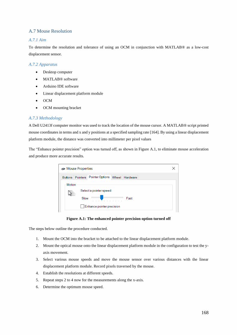
168
A.7 Mouse Resolution
A.7.1 Aim
To determine the resolution and tolerance of using an OCM in conjunction with MATLAB® as a low-cost
displacement sensor.
A.7.2 Apparatus
• Desktop computer
• MATLAB® software
• Arduino IDE software
• Linear displacement platform module
• OCM
• OCM mounting bracket
A.7.3 Methodology
A Dell U2413f computer monitor was used to track the location of the mouse cursor. A MATLAB® script printed
mouse coordinates in terms and x and y positions at a specified sampling rate [164]. By using a linear displacement
platform module, the distance was converted into millimeter per pixel values
The “Enhance pointer precision” option was turned off, as shown in Figure A.1, to eliminate mouse acceleration
and produce more accurate results.
Figure A.1: The enhanced pointer precision option turned off
The steps below outline the procedure conducted.
1. Mount the OCM into the bracket to be attached to the linear displacement platform module.
2. Mount the optical mouse onto the linear displacement platform module in the configuration to test the y-
axis movement.
3. Select various mouse speeds and move the mouse sensor over various distances with the linear
displacement platform module. Record pixels traversed by the mouse.
4. Establish the resolutions at different speeds.
5. Repeat steps 2 to 4 now for the measurements along the x-axis.
6. Determine the optimum mouse speed.

169
A.7.4 Results
The pitch of the ball screw shaft was 5 mm therefore the stepper motor was programmed to perform a specific
number of revolutions to meet the required linear displacements. Figure A.2. illustrates the different mounting
orientations of the OCM and the linear displacement platform module.
Figure A.2: Testing the OCM along the x and y axes
a. Resolution testing along the y-axis
b. Resolution testing along the x-axis
Table A.24 displays the summarised results of the OCM pixel resolution testing. Table A.25 shows the standard
deviations from the mean pixels recorded.
Table A.24: A summary of results for the OCM pixel resolution testing
Mouse
Speed
Direction Average resolution
(mm/pixel)
Average of X and Y
average resolution
2 X 1.63 1.64
2 Y 1.64
3 X 0.79 0.81
3 Y 0.82
4 X 0.2 0.2
4 Y 0.2
5 X 0.1 0.1
5 Y 0.1
6 X 0.07 0.07
6 Y 0.07
a. b.

170
Table A.25: Standard deviations from the mean pixels recorded
Speed 2
Distance (mm) 3 standard deviations X axis (pixels) 3 standard deviations Y axis (pixels)
5 0 1
10 1.06 1.92
15 1.45 1
20 1.57 1.21
40 2.26 2.66
Speed 3
Distance (mm) 3 standard deviations X axis (pixels) 3 standard deviations Y axis (pixels)
5 0.97 0.9
10 1.54 1.73
15 1.13 0.95
20 0.9 2.12
40 2.12 1.22
Speed 4
Distance (mm) 3 standard deviations X axis (pixels) 3 standard deviations Y axis (pixels)
5 2.15 1.78
10 3.17 3.42
15 5.41 3.09
20 4.53 2.12
40 5.32 5.07
Speed 5
Distance (mm) 3 standard deviations X axis (pixels) 3 standard deviations Y axis (pixels)
5 3.44 3.36
10 6.81 3.56
15 8.05 4.11
20 10.3 4.7
40 8.9 8.61
Speed 6
Distance (mm) 3 standard deviations X axis (pixels) 3 standard deviations Y axis (pixels)
5 7.61 4.3
10 12.21 4.9
15 17.54 9.48
20 17.89 7.72
40 15.7 13.18

171
A.7.5 Analysis
The mouse speed 2 was not considered because it did not yield a sub-millimeter resolution. Mouse speed 3 was
not used because it produced a resolution of 0.81mm/pixel, which was close to 1 mm. Mouse speed 5 and 6 yielded
sub-millimeter resolutions but the high sensitivity setting of the mouse required more monitor pixels than what
was available and was therefore not used. Moreover, the standard deviations increase with mouse speed, as
displayed in Table A.25. The three standard deviations from the mean showed a difference of approximately 5
pixels between speed 4 and speed 5 and showed a difference of approximately 12.5 pixels between speed 4 and
speed 6. Speed 4 is the best trade-off between resolution and monitor size and between resolution and 3 standard
deviations.
Three standard deviations from the mean for speed 4 is has a maximum number of 5.32 pixels at a travel distance
of 40 mm. In perspective, this relates to a tolerance of 1.06 mm from the mean. The three standard deviations
from the mean increases with distances therefore at distances travelled greater than 40 mm the deviation from the
predicted value of the PKM’s position may vary slightly more than 1.06 mm.
The advantages of using an OCM as a displacement sensor was that it was cost-effective and could easily interface
with the computer. The OCM is readily available with short lead times to obtain one. One of the disadvantages
was that it could only be used to measure translation of the end effector and not rotation. Another disadvantage
was that brackets had to be specifically designed to house the sensor to test the resolution of the mouse and for
the translation testing of the PKM. A linear displacement platform module was required to test the mouse
resolution which is not freely available to all researchers. Another challenge using an OCM as a displacement
sensor was that it only functioned appropriately when moving along a flat surface which required additional
designs to the testing system to accommodate this.
A.7.6 Conclusion
The OCM proved to be a viable low-cost displacement sensor when used with MATLAB®. Speed 4 was the best
speed setting and the pointer precision enhancement was turned off. A resolution of 0.2mm/pixel was obtained.
A tolerance of 1.06 mm was carried forward for physical testing.
A.7.7 Testing Data for Mouse Resolution Testing
Table A.26 to Table A.35 presents the pixels obtained and resulting resolution from testing the OCM. The mouse
was moved in increments of 5, 10, 15, 20 and 40 mm. The pixel position was recorded at the start of each
movement and the pixel difference between incremental movements was recorded. The mouse was moved
accurately in reality by the specified increments through the use of the linear displacement platform module.
Table A.26: Y-axis pixel displacements for Mouse Speed 2
5 mm Δ Pixel 10 mm Δ Pixel 15 mm Δ Pixel 20 mm Δ
Pixel
40 mm Δ Pixel
700 N/A 433 N/A 983 N/A 858 N/A 93 N/A
703 3 426 7 974 9 846 12 118 25
706 3 420 6 965 9 833 13
709 3 414 6 956 9 821 12 904 N/A

172
5 mm Δ Pixel 10 mm Δ Pixel 15 mm Δ Pixel 20 mm Δ
Pixel
40 mm Δ Pixel
712 3 946 10 809 12 881 23
715 3 239 N/A 937 9 856 25
719 4 246 7 147 N/A
722 3 251 5 40 N/A 159 12 38 N/A
725 3 257 6 49 9 172 13 63 25
728 3 263 6 58 9 184 12
269 6 67 9 1055 N/A
76 9 1019 N/A 1031 24
1007 12 1007 24
995 12
983 12 21 N/A
971 12 46 25
69 23
Average 3.11 6.13 9.11 12.18 24.25
Resolution 1.61 1.63 1.65 1.64 1.65
Average
Resolution 1.64
Table A.27: Y-axis pixel displacements for Mouse Speed 3
5 mm Δ
Pixel
10 mm Δ Pixel 15 mm Δ
Pixel
20 mm Δ
Pixel
40 mm Δ
Pixel
981 N/A 28 N/A 124 N/A 45 N/A 1075 N/A
975 6 41 13 142 18 69 24 1026 49
969 6 54 13 160 18 94 25
963 6 66 12 178 18 117 23 181 N/A
957 6 78 12 196 18 142 25 230 49
950 7 90 12
944 6 102 12 1104 N/A 1097 N/A 1065 N/A
938 6 114 12 1086 18 1073 24 1016 49
932 6 126 12 1068 18 1049 24 966 50
926 6
1050 18 1024 25
920 6 1049 N/A 1032 18 1000 24 54 N/A
914 6 1037 12 1013 19 975 25 103 49
1025 12 995 18
152 49
1014 11
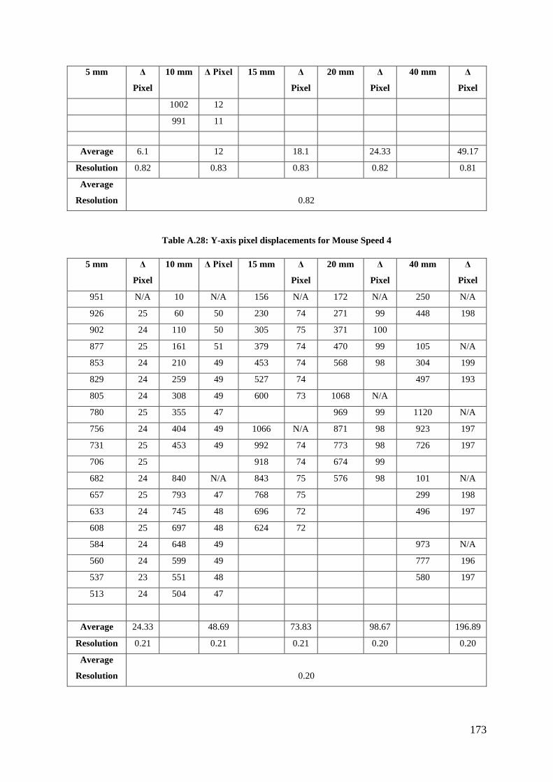
173
5 mm Δ
Pixel
10 mm Δ Pixel 15 mm Δ
Pixel
20 mm Δ
Pixel
40 mm Δ
Pixel
1002 12
991 11
Average 6.1
12
18.1
24.33
49.17
Resolution 0.82
0.83
0.83
0.82
0.81
Average
Resolution 0.82
Table A.28: Y-axis pixel displacements for Mouse Speed 4
5 mm Δ
Pixel
10 mm Δ Pixel 15 mm Δ
Pixel
20 mm Δ
Pixel
40 mm Δ
Pixel
951 N/A 10 N/A 156 N/A 172 N/A 250 N/A
926 25 60 50 230 74 271 99 448 198
902 24 110 50 305 75 371 100
877 25 161 51 379 74 470 99 105 N/A
853 24 210 49 453 74 568 98 304 199
829 24 259 49 527 74
497 193
805 24 308 49 600 73 1068 N/A
780 25 355 47
969 99 1120 N/A
756 24 404 49 1066 N/A 871 98 923 197
731 25 453 49 992 74 773 98 726 197
706 25
918 74 674 99
682 24 840 N/A 843 75 576 98 101 N/A
657 25 793 47 768 75
299 198
633 24 745 48 696 72
496 197
608 25 697 48 624 72
584 24 648 49
973 N/A
560 24 599 49
777 196
537 23 551 48
580 197
513 24 504 47
Average 24.33
48.69
73.83
98.67
196.89
Resolution 0.21
0.21
0.21
0.20
0.20
Average
Resolution 0.20

174
Table A.29: Y-axis pixel displacements for Mouse Speed 5
5 mm Δ
Pixel
10 mm Δ Pixel 15 mm Δ
Pixel
20 mm Δ
Pixel
40 mm Δ
Pixel
1062 N/A 72 N/A 13 N/A 202 N/A 1061 N/A
1012 50 170 98 158 145 397 195 662 399
964 48 269 99 306 148 595 198 269 393
915 49 368 99 454 148 792 197
866 49 466 98 600 146
388
817 49 564 98 746 146 1115 N/A 785 397
768 49 663 99
921 194
721 47 759 96 1082 N/A 723 198 995 N/A
673 48 856 97 933 149 526 197 603 392
624 49
785 148 330 196 207 396
578 46 966 N/A 638 147
529 49 868 98
429 N/A 129 N/A
482 47 772 96 796 N/A 627 198 524 395
434 48 675 97 649 147 821 194 915 391
385 49 579 96 504 145 1017 196
338 47 480 99
288 50 381 99
239 49 282 99
Average 48.41
97.87
146.9
196.3
394.71
Resolution 0.10
0.10
0.10
0.10
0.10
Average
Resolution 0.10
Table A.30: Y-axis pixel displacements for Mouse Speed 6
5 mm Δ Pixel 10 mm Δ Pixel 15 mm Δ Pixel 20 mm Δ
Pixel
40 mm Δ
Pixel
983 N/A 107 N/A 245 N/A 132 N/A 279 N/A
912 71 254 147 473 228 426 294 868 589
839 73 402 148 696 223 717 291
765 74 550 148 920 224 1014 297 872 N/A
691 74 698 148 1144 224
273 599
615 76 846 148
906 N/A
541 74 992 146 953 N/A 609 297 161 N/A
467 74 1137 145 731 222 316 293 749 588

175
5 mm Δ Pixel 10 mm Δ Pixel 15 mm Δ Pixel 20 mm Δ
Pixel
40 mm Δ
Pixel
510 221 24 292
323 N/A 894 N/A 292 218
882 N/A
250 73 748 146 73 219 998 N/A 292 590
176 74 597 151
707 291
105 71 450 147
1170 N/A
32 73 301 149
578 592
Average 73.36
147.55
222.38
293.5
7
591.6
Resolution 0.07
0.07
0.07
0.07
0.07
Average
Resolution 0.07
Table A.31: X-axis pixel displacements for Mouse Speed 2
5 mm Δ Pixel 10 mm Δ Pixel 15 mm Δ Pixel 20 mm Δ
Pixel
40 mm Δ
Pixel
50 N/A 214 N/A -1788 N/A 965 N/A -935 N/A
53 3 220 6 -1797 9 952 13 -961 26
56 3 226 6 -1806 9 940 12
59 3 232 6 -1816 10 927 13 -1101 N/A
62 3 239 7 -1825 9 914 13 -1076 25
65 3 245 6 -1835 10 902 12 -1052 24
68 3 251 6 -1844 9
71 3 257 6
-783 N/A -1145 N/A
74 3 263 6 719 N/A -771 12 -1170 25
77 3 269 6 728 9 -759 12
80 3
-747 12 -870 N/A
83 3
756 N/A -734 13 -846 24
86 3
765 9 -722 12 -821 25
89 3
775 10 -709 13
92 3
784 9
Average 3
6.13
9.3
12.45
24.83
Resolution 1.67
1.63
1.61
1.61
1.61
Average
Resolution 1.63

176
Table A.32: X-axis pixel displacements for Mouse Speed 3
5 mm Δ Pixel 10 mm Δ Pixel 15 mm Δ
Pixel
20 mm Δ
Pixel
40 mm Δ
Pixel
-763 N/A 793 N/A -877 N/A -1162 N/A 1029 N/A
-769 6 781 12 -895 18 -1187 25 979 50
-775 6 768 13 -914 19 -1212 25 929 50
-781 6 755 13 -933 19 -1237 25
-787 6 743 12 -952 19 -1262 25 943 N/A
-793 6 730 13 -971 19
993 50
-799 6 717 13 -990 19 959 N/A 1043 50
-805 6 705 12 -1009 19 983 24 1093 50
-812 7 692 13
1008 25
-818 6 680 12 -912 N/A 1033 25 897 N/A
-824 6 667 13 -894 18 1058 25 848 49
-830 6
-875 19 1033 25 797 51
-836 6 920 N/A -856 19 1058 25
-843 7 932 12 -837 19 1083 25 1044 N/A
-849 6 944 12 -818 19
1093 49
-855 6 957 13 -799 19
1144 51
-861 6 970 13
-867 6 982 12
-873 6 995 13
Average 6.11
12.56
18.84
24.91
50
Resolution 0.82
0.80
0.80
0.80
0.80
Average
Resolution 0.80
Table A.33: X-axis pixel displacements for Mouse Speed 4
5 mm Δ Pixel 10 mm Δ Pixel 15 mm Δ
Pixel
20 mm Δ
Pixel
40 mm Δ
Pixel
965 N/A 991 N/A 1432 N/A 1226 N/A 1053 N/A
941 24 1040 49 1505 73 1326 100 1256 203
916 25 1091 51 1580 75 1427 101 1456 200
892 24 1141 50
1529 102
867 25 1192 51 805 N/A 1628 99 672 N/A
843 24 1243 51 733 72
469 203
819 24 1293 50 657 76 833 N/A 267 202

177
5 mm Δ Pixel 10 mm Δ Pixel 15 mm Δ
Pixel
20 mm Δ
Pixel
40 mm Δ
Pixel
794 25 1342 49 581 76 735 98
770 24 1391 49 506 75 632 103 1129 N/A
745 25 1440 49 428 78 531 101 1331 202
720 25
352 76 431 100
695 25 947 N/A 278 74 331 100 667 N/A
670 25 898 49
467 200
644 26 849 49
262 205
619 25 799 50
594 25 748 51
568 26 696 52
544 24 646 50
518 26 594 52
493 25 544 50
467 26 495 49
Average 24.9
50.06
75
100.4
4
202.14
Resolution 0.20
0.20
0.20
0.20
0.20
Average
Resolution 0.20
Table A.34: X-axis pixel displacements for Mouse Speed 5
5 mm Δ Pixel 10 mm Δ Pixel 15 mm Δ
Pixel
20 mm Δ
Pixel
40 mm Δ
Pixel
832 N/A 767 N/A 272 N/A 27 N/A 309 N/A
881 49 670 97 125 147 -174 201 -87 396
930 49 572 98 -24 149 -377 203 -490 403
979 49 472 100 -178 154 -580 203
1028 49 368 104 -328 150 -779 199 587 N/A
1078 50 267 101 -479 151 -976 197 989 402
1128 50 165 102 -629 150
1388 399
1177 49 62 103 -779 150 399 N/A
1229 52 -39 101
596 197 1718 N/A
1280 51 -140 101 377 N/A 798 202 1316 402
1332 52 -236 96 522 145 1005 207 912 404
1382 50
675 153 1209 204

178
5 mm Δ Pixel 10 mm Δ Pixel 15 mm Δ
Pixel
20 mm Δ
Pixel
40 mm Δ
Pixel
1432 50 314 N/A 824 149 1406 197
1482 50 411 97 977 153
1532 50 511 100 1126 149
1584 52 609 98 1273 147
1635 51 711 102 1419 146
1684 49 812 101
1733 49 915 103
1783 50 1015 100
1831 48 1116 101
Average 49.95
100.28
149.5
201
401
Resolution 0.10
0.10
0.10
0.10
0.10
Average
Resolution 0.10
Table A.35: X-axis pixel displacements for Mouse Speed 6
5 mm Δ Pixel 10 mm Δ Pixel 15 mm Δ
Pixel
20 mm Δ
Pixel
40 mm Δ
Pixel
-57 N/A 532 N/A 282 N/A 145 N/A 1807 N/A
-128 71 676 144 477 195 436 291 1215 592
-199 71 816 140 681 204 730 294 625 590
-272 73 950 134 892 211 1015 285
-344 72 1086 136 1098 206 1305 290 387 N/A
-413 69 1222 136 1310 212 1596 291 992 605
-483 70 1357 135 1517 207 1597 605
-553 70 1595 N/A
-623 70 -261 N/A 1800 N/A 1300 295 -434 N/A
-697 74 -401 140 1589 211 1003 297 -1035 601
-769 72 -541 140 1377 212 700 303
-842 73 -677 136 1166 211 401 299 189 N/A
-912 70 -818 141 951 215 795 606
-978 66 -963 145 739 212 1530 N/A 1392 597
-1044 66 -1107 144 540 199 1232 298
-1110 66 -1243 136 328 212 930 302 1351 N/A
-1179 69 -1375 132 625 305 749 602
-1246 67 323 302 146 603

179
5 mm Δ Pixel 10 mm Δ Pixel 15 mm Δ
Pixel
20 mm Δ
Pixel
40 mm Δ
Pixel
133 N/A
733 600
1332 599
Average 69.94 138.5 208.2
3077
296.3
0769
600
Resolution 0.07 0.07 0.07 0.07 0.07
Average
Resolution 0.071
Figure A.3 to Figure A.7 presents the 3 standard deviations of pixel measurements versus distance travelled.
Figure A.3: Graph of OCM Speed 2: 3 Standard Deviations of Pixel Measurements vs. Distance Travelled
0
0,5
1
1,5
2
2,5
3
0 5 10 15 20 25 30 35 40 45
3 S
tan
dar
d D
evia
tio
ns
of
Pix
el
Mea
sure
men
ts (
pix
els)
Distance Travelled (mm)
OCM Speed 2: 3 Standard Deviations of Pixel Measurements vs Distance Travelled
X axis Y Axis

180
Figure A.4: Graph of OCM Speed 3: 3 Standard Deviations of Pixel Measurements vs. Distance Travelled
Figure A.5: Graph of OCM Speed 4: 3 Standard Deviations of Pixel Measurements vs. Distance Travelled
0
0,5
1
1,5
2
2,5
0 5 10 15 20 25 30 35 40 45
3 S
tan
dar
d D
evia
tio
ns
of
Pix
el
Mea
sure
men
ts (
pix
els)
Distance Travelled (mm)
OCM Speed 3: 3 Standard Deviations of Pixel Measurements vs Distance Travelled
X Axis Y Axis
0
1
2
3
4
5
6
0 5 10 15 20 25 30 35 40 45
3 S
tan
dar
d D
evia
tio
ns
of
Pix
el
Mea
sure
men
ts (
pix
els)
Distance Travelled (mm)
OCM Speed 4: 3 Standard Deviations of Pixel Measurements vs Distance Travelled
X Axis Y Axis

181
Figure A.6: Graph of OCM Speed 5: 3 Standard Deviations of Pixel Measurements vs. Distance Travelled
Figure A.7: Graph of OCM Speed 6: 3 Standard Deviations of Pixel Measurements vs. Distance Travelled
0
2
4
6
8
10
12
0 5 10 15 20 25 30 35 40 45
3 S
tan
dar
d D
evia
tio
ns
of
Pix
el
Mea
sure
men
ts (
pix
els)
Distance Travelled (mm)
OCM Speed 5: 3 Standard Deviations of Pixel Measurements vs Distance Travelled
X Axis Y Axis
0
5
10
15
20
0 5 10 15 20 25 30 35 40 45
3 S
tan
dar
d D
evia
tio
ns
of
Pix
el
Mea
sure
men
ts (
pix
els)
Distance Travelled (mm)
OCM Speed 6: 3 Standard Deviations of Pixel Measurements vs Distance Travelled
X Axis Y Axis

182
Appendix B – Code from Software
B.1 Inverse Kinematics: MATLAB® Code
B.1.1 Main script file
%Inverse kinematics of the 5 DOF PKM
%Inputs d2r=pi/180;
alpha=20*d2r; beta=0*d2r; gamma=0*d2r;
xf=111.36; yf=-53.27; zf=311.04;
%End Effector inputs ('f' = final) OPPORG=[xf; yf; zf];
ROP=RotationalMatrix(alpha,beta,gamma);
%Machine parameters %Leg 1 PPDORG1=[-19.34; -33.50; 0]; OPAORG1=[-75; -129.9; 0]; AB1=[61.5; 0; 85]; %thrust bearing measurements DC1=[43; 0; 40]; PPDORG1top=[-19.34; -33.50; 12]; PPDORG1bottom=[-19.34; -33.50; -12];
%Leg 2 PPDORG2=PPDORG1; OPAORG2=OPAORG1; AB2=[41.5; 0; 165]; % thrust bearing measurements DC2=[63; 0; -40]; PPDORG2top=PPDORG1top; PPDORG2bottom=PPDORG1bottom;
%Leg 3 PPDORG3=[-19.34; 33.50; 0]; OPAORG3=[-75; 129.9; 0]; AB3=AB1; DC3=DC1; PPDORG3top=[-19.34; 33.50; 12]; PPDORG3bottom=[-19.34; 33.50; -12];
%Leg 4 PPDORG4=PPDORG3; OPAORG4=OPAORG3; AB4=AB2; DC4=DC2; PPDORG4top=PPDORG3top; PPDORG4bottom=PPDORG3bottom;
%Leg 5 PPDORG5=[38.69; -25; 0];

183
OPAORG5=[150; 0; 60]; AB5=[0; -40; 22.5]; DC5=[0; 15; 22.5];
%Leg 6 PPDORG6=[38.69; 25; 0]; OPAORG6=OPAORG5; AB6=[0; 40; 22.5]; DC6=[0; -15; 22.5];
%%%%%%%%%%%%%%%%%%%%%%%%%%%%%%%%%%%%%%%%%%%%%%%%%%%%%%%%%%%%%%%%%% %General Actuator 1 Calculations %AD1 Calculation AD1=OPPORG+(ROP*PPDORG1)-OPAORG1; MagAD1=norm(AD1);
AD1top=OPPORG+(ROP*PPDORG1top)-OPAORG1; MagAD1top=norm(AD1top);
AD1bottom=OPPORG+(ROP*PPDORG1bottom)-OPAORG1; MagAD1bottom=norm(AD1bottom);
%Location of point D xA1=sqrt((MagAD1^2)-(AD1(3,1))^2); xzAD1=[xA1; 0; AD1(3,1)];
xA1top=sqrt((MagAD1top^2)-(AD1top(3,1))^2); xzAD1top=[xA1top; 0; AD1top(3,1)];
xA1bottom=sqrt((MagAD1bottom^2)-(AD1bottom(3,1))^2); xzAD1bottom=[xA1bottom; 0; AD1bottom(3,1)];
%General Actuator 2 Calculations %AD2 Calculation AD2=AD1; AD2top=AD1top; AD2bottom=AD1bottom;
MagAD2=MagAD1; MagAD2top=MagAD1top; MagAD2bottom=MagAD1bottom;
%Location of point D xA2=xA1; xzAD2=xzAD1;
xA2top=xA1top; xzAD2top=xzAD1top;
xA2bottom=xA1bottom; xzAD2bottom=xzAD1bottom;
%General Actuator 3 Calculations %AD3 Calculation AD3=OPPORG+(ROP*PPDORG3)-OPAORG3; MagAD3=norm(AD3);

184
AD3top=OPPORG+(ROP*PPDORG3top)-OPAORG3; MagAD3top=norm(AD3top);
AD3bottom=OPPORG+(ROP*PPDORG3bottom)-OPAORG3; MagAD3bottom=norm(AD3bottom);
%Location of point D xA3=sqrt((MagAD3^2)-(AD3(3,1))^2); xzAD3=[xA3; 0; AD3(3,1)];
xA3top=sqrt((MagAD3top^2)-(AD3top(3,1))^2); xzAD3top=[xA3top; 0; AD3top(3,1)];
xA3bottom=sqrt((MagAD3bottom^2)-(AD3bottom(3,1))^2); xzAD3bottom=[xA3bottom; 0; AD3bottom(3,1)];
%General Actuator 4 Calculations %AD3 Calculation AD4=AD3; AD4top=AD3top; AD4bottom=AD3bottom;
MagAD4=MagAD3; MagAD4top=MagAD3top; MagAD4bottom=MagAD3bottom;
%Location of point D xA4=xA3; xzAD4=xzAD3;
xA4top=xA3top; xzAD4top=xzAD3top;
xA4bottom=xA3bottom; xzAD4bottom=xzAD3bottom;
%General Actuator 5 Calculations %AD5 Calculation AD5=OPPORG+(ROP*PPDORG5)-OPAORG5; MagAD5=norm(AD5);
%Location of point D zA5=sqrt((MagAD5^2)-(AD5(2,1))^2); yzAD5=[0; AD5(2,1); zA5];
%General Actuator 6 Calculations %AD6 Calculation AD6=OPPORG+(ROP*PPDORG6)-OPAORG6; MagAD6=norm(AD6);
%Location of point D zA6=sqrt((MagAD6^2)-(AD6(2,1))^2); yzAD6=[0; AD6(2,1); zA6];
%%%%%%%%%%%%%%%%%%%%%%%%%%%%%%%%%%%%%%%%%%%%%%%%%%%%%%%%%%%%%%%%%%%%%%%%%%% %Leg lengths by Cases if beta>0 %12bracket leans Forward and 34bracket leans Forward

185
[Length1,Length2]=PosGrad12(d2r,xzAD1top,xzAD1bottom,DC1,xzAD1,AB1,DC2,xzAD
2,AB2);
[Length3,Length4]=PosGrad34(d2r,xzAD3top,xzAD3bottom,DC3,xzAD3,AB3,DC4,xzAD
4,AB4);
BC5=yzAD5-AB5-DC5; Length5=norm(BC5);
BC6=yzAD6-AB6-DC6; Length6=norm(BC6);
elseif beta <0 %12bracket leans Backward and 34bracket leans Backward
[Length1,Length2]=NegGrad12(d2r,xzAD1top,xzAD1bottom,DC1,xzAD1,AB1,DC2,xzAD
2,AB2);
[Length3,Length4]=NegGrad34(d2r,xzAD3top,xzAD3bottom,DC3,xzAD3,AB3,DC4,xzAD
4,AB4);
BC5=yzAD5-AB5-DC5; Length5=norm(BC5);
BC6=yzAD6-AB6-DC6; Length6=norm(BC6);
elseif alpha >0 gradient12=(xzAD1top(3,1)-xzAD1bottom(3,1))/(xzAD1top(1,1)-
xzAD1bottom(1,1)); gradient34=(xzAD3top(3,1)-xzAD3bottom(3,1))/(xzAD3top(1,1)-
xzAD3bottom(1,1));
[Length5,Length6]=PosGrad56(alpha,d2r,DC5,yzAD5,AB5,DC6,yzAD6,AB6);
if gradient12>0 && gradient34>0 %12bracket leans Forward and 34bracket
leans Forward
[Length1,Length2]=PosGrad12(d2r,xzAD1top,xzAD1bottom,DC1,xzAD1,AB1,DC2,xzAD
2,AB2);
[Length3,Length4]=PosGrad34(d2r,xzAD3top,xzAD3bottom,DC3,xzAD3,AB3,DC4,xzAD
4,AB4);
elseif gradient12<0 && gradient34>0 %12bracket leans Backward and
34bracket leans Forward
[Length1,Length2]=NegGrad12(d2r,xzAD1top,xzAD1bottom,DC1,xzAD1,AB1,DC2,xzAD
2,AB2);
[Length3,Length4]=PosGrad34(d2r,xzAD3top,xzAD3bottom,DC3,xzAD3,AB3,DC4,xzAD
4,AB4);
elseif gradient12<0 && gradient34<0 %12bracket leans Backward and
34bracket leans Backward
[Length1,Length2]=NegGrad12(d2r,xzAD1top,xzAD1bottom,DC1,xzAD1,AB1,DC2,xzAD
2,AB2);

186
[Length3,Length4]=NegGrad34(d2r,xzAD3top,xzAD3bottom,DC3,xzAD3,AB3,DC4,xzAD
4,AB4);
elseif xzAD1top(1,1) == xzAD1bottom(1,1) %12bracket stands Upright and
34bracket leans Forward
BC1=xzAD1-AB1-DC1; Length1=norm(BC1);
BC2=xzAD2-AB2-DC2; Length2=norm(BC2);
[Length3,Length4]=PosGrad34(d2r,xzAD3top,xzAD3bottom,DC3,xzAD3,AB3,DC4,xzAD
4,AB4);
elseif xzAD3top(1,1) == xzAD3bottom(1,1) %12bracket leans Backward and
34bracket stands Upright
[Length1,Length2]=NegGrad12(d2r,xzAD1top,xzAD1bottom,DC1,xzAD1,AB1,DC2,xzAD
2,AB2); BC3=xzAD3-AB3-DC3; Length3=norm(BC3);
BC4=xzAD4-AB4-DC4; Length4=norm(BC4);
end
elseif alpha<0 gradient12=(xzAD1top(3,1)-xzAD1bottom(3,1))/(xzAD1top(1,1)-
xzAD1bottom(1,1)); gradient34=(xzAD3top(3,1)-xzAD3bottom(3,1))/(xzAD3top(1,1)-
xzAD3bottom(1,1));
[Length5,Length6]=NegGrad56(alpha,d2r,DC5,yzAD5,AB5,DC6,yzAD6,AB6);
if gradient12>0 && gradient34<0 %12bracket leans Forward and 34bracket
leans Backward
[Length1,Length2]=PosGrad12(d2r,xzAD1top,xzAD1bottom,DC1,xzAD1,AB1,DC2,xzAD
2,AB2);
[Length3,Length4]=NegGrad34(d2r,xzAD3top,xzAD3bottom,DC3,xzAD3,AB3,DC4,xzAD
4,AB4);
elseif gradient12>0 && gradient34>0 %12bracket leans Forward and
34bracket leans Forward
[Length1,Length2]=PosGrad12(d2r,xzAD1top,xzAD1bottom,DC1,xzAD1,AB1,DC2,xzAD
2,AB2);
[Length3,Length4]=PosGrad34(d2r,xzAD3top,xzAD3bottom,DC3,xzAD3,AB3,DC4,xzAD
4,AB4);
elseif gradient12<0 && gradient34<0 %12bracket leans Backward and
34bracket leans Backward

187
[Length1,Length2]=NegGrad12(d2r,xzAD1top,xzAD1bottom,DC1,xzAD1,AB1,DC2,xzAD
2,AB2);
[Length3,Length4]=NegGrad34(d2r,xzAD3top,xzAD3bottom,DC3,xzAD3,AB3,DC4,xzAD
4,AB4);
elseif xzAD1top(1,1) == xzAD1bottom(1,1) %12bracket stands Upright and
34bracket leans Backward %Length1 BC1=xzAD1-AB1-DC1; Length1=norm(BC1);
%Length2 BC2=xzAD2-AB2-DC2; Length2=norm(BC2);
[Length3,Length4]=NegGrad34(d2r,xzAD3top,xzAD3bottom,DC3,xzAD3,AB3,DC4,xzAD
4,AB4);
elseif xzAD3top(1,1) == xzAD3bottom(1,1) %12bracket leans Forward and
34bracket stands Upright
[Length1,Length2]=PosGrad12(d2r,xzAD1top,xzAD1bottom,DC1,xzAD1,AB1,DC2,xzAD
2,AB2); BC3=xzAD3-AB3-DC3; Length3=norm(BC3);
BC4=xzAD4-AB4-DC4; Length4=norm(BC4);
end
elseif beta==0 && alpha==0 %Inner Vector loops %Length1 BC1=xzAD1-AB1-DC1; Length1=norm(BC1);
%Length2 BC2=xzAD2-AB2-DC2; Length2=norm(BC2);
%Length3 BC3=xzAD3-AB3-DC3; Length3=norm(BC3);
%Length4 BC4=xzAD4-AB4-DC4; Length4=norm(BC4);
%Length5 BC5=yzAD5-AB5-DC5; Length5=norm(BC5);
%Length6 BC6=yzAD6-AB6-DC6; Length6=norm(BC6); end

188
B.1.2 Function file – Rotational Matrix
function [ROP]=RotationalMatrix(alpha,beta,gamma) ROP=[cos(gamma)*cos(beta) (cos(gamma)*sin(beta)*sin(alpha))-
(sin(gamma)*cos(alpha))
(cos(gamma)*sin(beta)*cos(alpha))+(sin(gamma)*sin(alpha));... sin(gamma)*cos(beta)
(sin(gamma)*sin(beta)*sin(alpha))+(cos(gamma)*cos(alpha))
(sin(gamma)*sin(beta)*cos(alpha))-(cos(gamma)*sin(alpha));... -sin(beta) cos(beta)*sin(alpha) cos(beta)*cos(alpha)]; end
B.1.3 Function file – Negative gradient of the Joint D bracket for leg 1 and 2
function
[Length1,Length2]=NegGrad12(d2r,xzAD1top,xzAD1bottom,DC1,xzAD1,AB1,DC2,xzAD
2,AB2) %Length1 gradient12=(xzAD1top(3,1)-xzAD1bottom(3,1))/(xzAD1top(1,1)-
xzAD1bottom(1,1)); radgradient12=atan(gradient12); deggradient12=radgradient12/d2r+180;
MagDC1 = sqrt((DC1(1,1)^2)+(DC1(3,1))^2); gradientDC1=(DC1(3,1))/(DC1(1,1)); radinnerangleDC1=atan(gradientDC1); deginnerangleDC1=90-radinnerangleDC1/d2r;
theta1=deggradient12-deginnerangleDC1; DC1rotated=[MagDC1*cos(theta1*d2r); 0; MagDC1*sin(theta1*d2r)]
BC1=xzAD1-AB1-DC1rotated;
Length1=norm(BC1);
%Length2 MagDC2 = sqrt((DC2(1,1)^2)+(DC2(3,1))^2); gradientDC2=(DC2(3,1))/(DC2(1,1)); radinnerangleDC2=atan(gradientDC2); deginnerangleDC2=90+radinnerangleDC2/d2r;
theta2=180-deggradient12-deginnerangleDC2; DC2rotated=[MagDC2*cos(theta2*d2r); 0; -MagDC2*sin(theta2*d2r)]
BC2=xzAD2-AB2-DC2rotated;
Length2=norm(BC2); end
B.1.4 Function file – Negative gradient of the Joint D bracket for leg 3 and 4
function
[Length3,Length4]=NegGrad34(d2r,xzAD3top,xzAD3bottom,DC3,xzAD3,AB3,DC4,xzAD
4,AB4) %Length3 gradient34=(xzAD3top(3,1)-xzAD3bottom(3,1))/(xzAD3top(1,1)-
xzAD3bottom(1,1)); radgradient34=atan(gradient34);

189
deggradient34=radgradient34/d2r+180;
MagDC3 = sqrt((DC3(1,1)^2)+(DC3(3,1))^2); gradientDC3=(DC3(3,1))/(DC3(1,1)); radinnerangleDC3=atan(gradientDC3); deginnerangleDC3=90-radinnerangleDC3/d2r;
theta3=deggradient34-deginnerangleDC3; DC3rotated=[MagDC3*cos(theta3*d2r); 0; MagDC3*sin(theta3*d2r)]
BC3=xzAD3-AB3-DC3rotated;
Length3=norm(BC3);
%Length4 MagDC4 = sqrt((DC4(1,1)^2)+(DC4(3,1))^2); gradientDC4=(DC4(3,1))/(DC4(1,1)); radinnerangleDC4=atan(gradientDC4); deginnerangleDC4=90+radinnerangleDC4/d2r;
theta4=180-deggradient34-deginnerangleDC4; DC4rotated=[MagDC4*cos(theta4*d2r); 0; -MagDC4*sin(theta4*d2r)]
BC4=xzAD4-AB4-DC4rotated;
Length4=norm(BC4); end
B.1.5 Function file – Negative gradient of the end effector for alpha rotations
function [Length5,Length6]=NegGrad56(alpha,d2r,DC5,yzAD5,AB5,DC6,yzAD6,AB6) %Length 5 deggradient56=90+alpha/d2r;
MagDC5 = sqrt((DC5(2,1)^2)+(DC5(3,1))^2); gradientDC5=(DC5(3,1))/(DC5(2,1)); radinnerangleDC5=atan(gradientDC5); deginnerangleDC5=90-radinnerangleDC5/d2r;
theta5=deggradient56-deginnerangleDC5; DC5rotated=[0; MagDC5*cos(theta5*d2r); MagDC5*sin(theta5*d2r)]
BC5=yzAD5-AB5-DC5rotated; Length5=norm(BC5);
%Length 6 MagDC6=MagDC5; gradientDC6=(DC6(3,1))/(DC6(2,1)); radinnerangleDC6=atan(gradientDC6); deginnerangleDC6=radinnerangleDC6/d2r;
theta6=-(deginnerangleDC6+alpha/d2r); DC6rotated=[0; -MagDC6*cos(theta6*d2r); MagDC6*sin(theta6*d2r)]
BC6=yzAD6-AB6-DC6rotated; Length6=norm(BC6); end

190
B.1.6 Function file – Positive gradient of the Joint D bracket for leg 1 and 2
function
[Length1,Length2]=PosGrad12(d2r,xzAD1top,xzAD1bottom,DC1,xzAD1,AB1,DC2,xzAD
2,AB2) %Actuator 1 %Top Bracket gradient calculation gradient12=(xzAD1top(3,1)-xzAD1bottom(3,1))/(xzAD1top(1,1)-
xzAD1bottom(1,1)); radgradient12=atan(gradient12); deggradient12=radgradient12/d2r;
MagDC1 = sqrt((DC1(1,1)^2)+(DC1(3,1))^2); gradientDC1=(DC1(3,1))/(DC1(1,1)); radinnerangleDC1=atan(gradientDC1); deginnerangleDC1=90-radinnerangleDC1/d2r;
theta1=deggradient12-deginnerangleDC1; DC1rotated=[MagDC1*cos(theta1*d2r); 0; MagDC1*sin(theta1*d2r)]
%Vector loop within a loop BC1=xzAD1-AB1-DC1rotated;
%Final Actuator Length Length1=norm(BC1);
%%%%%%%%%%%%%%%%%%%%%%%%%%%%%%%%%%%%%%%%%%%%%%%%%%%%%%%%%%%%%%%%%%% %Actuator 2 %Altered vector DC2 MagDC2 = sqrt((DC2(1,1)^2)+(DC2(3,1))^2); gradientDC2=(DC2(3,1))/(DC2(1,1)); radinnerangleDC2=atan(gradientDC2); deginnerangleDC2=90+radinnerangleDC2/d2r;
theta2=180-deggradient12-deginnerangleDC2; DC2rotated=[MagDC2*cos(theta2*d2r); 0; -MagDC2*sin(theta2*d2r)]
%Vector loop within a loop BC2=xzAD2-AB2-DC2rotated;
%Final Actuator Length Length2=norm(BC2); end
B.1.7 Function file – Positive gradient of the Joint D bracket for leg 3 and 4
function
[Length3,Length4]=PosGrad34(d2r,xzAD3top,xzAD3bottom,DC3,xzAD3,AB3,DC4,xzAD
4,AB4) %Actuator 3 Length Calculations %Top Bracket gradient calculation gradient34=(xzAD3top(3,1)-xzAD3bottom(3,1))/(xzAD3top(1,1)-
xzAD3bottom(1,1)); radgradient34=atan(gradient34); deggradient34=radgradient34/d2r;
%Altered vector DC3 MagDC3 = sqrt((DC3(1,1)^2)+(DC3(3,1))^2); gradientDC3=(DC3(3,1))/(DC3(1,1));

191
radinnerangleDC3=atan(gradientDC3); deginnerangleDC3=90-radinnerangleDC3/d2r;
theta3=deggradient34-deginnerangleDC3; DC3rotated=[MagDC3*cos(theta3*d2r); 0; MagDC3*sin(theta3*d2r)]
%Vector loop within a loop BC3=xzAD3-AB3-DC3rotated;
%Final Actuator Length Length3=norm(BC3);
%%%%%%%%%%%%%%%%%%%%%%%%%%%%%%%%%%%%%%%%%%%%%%%%%%%%%%%%%%%%%%%%%%% %Actuator 4 %Altered vector DC4 MagDC4 = sqrt((DC4(1,1)^2)+(DC4(3,1))^2); gradientDC4=(DC4(3,1))/(DC4(1,1)); radinnerangleDC4=atan(gradientDC4); deginnerangleDC4=90+radinnerangleDC4/d2r;
theta4=180-deggradient34-deginnerangleDC4; DC4rotated=[MagDC4*cos(theta4*d2r); 0; -MagDC4*sin(theta4*d2r)]
%Vector loop within a loop BC4=xzAD4-AB4-DC4rotated;
%Final Actuator Length Length4=norm(BC4); end
B.1.8 Function file – Positive gradient of the end effector for alpha rotations
function [Length5,Length6]=PosGrad56(alpha,d2r,DC5,yzAD5,AB5,DC6,yzAD6,AB6) %Length 5 deggradient56=alpha/d2r;
MagDC5 = sqrt((DC5(2,1)^2)+(DC5(3,1))^2); gradientDC5=(DC5(3,1))/(DC5(2,1)); radinnerangleDC5=atan(gradientDC5); deginnerangleDC5=90-radinnerangleDC5/d2r;
theta5=90-deginnerangleDC5+deggradient56; DC5rotated=[0; MagDC5*cos(theta5*d2r); MagDC5*sin(theta5*d2r)]
BC5=yzAD5-AB5-DC5rotated; Length5=norm(BC5);
%Length 6 MagDC6=MagDC5; gradientDC6=(DC6(3,1))/(DC6(2,1)); radinnerangleDC6=atan(gradientDC6); deginnerangleDC6=radinnerangleDC6/d2r;
theta6=-(deginnerangleDC6+(alpha/d2r)); DC6rotated=[0; -MagDC6*cos(theta6*d2r); MagDC6*sin(theta6*d2r)]
BC6=yzAD6-AB6-DC6rotated;

192
Length6=norm(BC6); end
B.1.9 Mouse tracker code
t = timer('ExecutionMode', 'fixedRate', ... 'Period', 0.1, ... %Sampling rate 'TasksToExecute', 900, ... 'TimerFcn', @(~,~) fprintf('(X, Y) = (%g, %g)\n', get(0,
'PointerLocation'))); start(t); %will display mouse movements for 90 seconds

193
B.2 Inverse Kinematics: Arduino Code
// MultiStepper.pde
// -*- mode: C++ -*-
// Use MultiStepper class to manage multiple steppers and make them all move to
// the same position at the same time for linear 2d (or 3d) motion.
#include <AccelStepper.h>
#include <MultiStepper.h> //The Multistepper is a sub-class of the AccelStepper library therefore only called
after the AccelStepper library
// EG X-Y position bed driven by two steppers
AccelStepper stepper1(1,2,3); //The first value in brackets '1' means that a driver is being used to power the
stepper, The 2nd (CLK) and 3rd (CW) values are the PWM pins on the Arduino.
AccelStepper stepper2(1,4,5);
AccelStepper stepper3(1,6,7);
AccelStepper stepper4(1,8,9);
AccelStepper stepper5(1,10,11);
AccelStepper stepper6(1,12,13);
// Up to 10 steppers can be handled as a group by MultiStepper
MultiStepper steppers;
void setup() {
Serial.begin(9600);
// Configure each stepper
stepper1.setMaxSpeed(200); //Steps per second
stepper2.setMaxSpeed(200);
stepper3.setMaxSpeed(200);
stepper4.setMaxSpeed(200);
stepper5.setMaxSpeed(200);
stepper6.setMaxSpeed(200);
// Then give them to MultiStepper to manage

194
steppers.addStepper(stepper1);
steppers.addStepper(stepper2);
steppers.addStepper(stepper3);
steppers.addStepper(stepper4);
steppers.addStepper(stepper5);
steppers.addStepper(stepper6);
}
void loop() {
long positions[6]; // Array of stepper positions
positions[0] = -5582; //references to a coordinate
positions[1] = -5582;
positions[2] = -5549;
positions[3] = -5549;
positions[4] = -9254;
positions[5] = -9254;
steppers.moveTo(positions);
steppers.runSpeedToPosition(); // Blocks until all are in position

195
B.3 Forward kinematics MATLAB® Code
B.3.1 Translation
syms OPx OPy OPz theta1 theta3 theta5
d2r=pi/180;
alpha = 0;
beta = 0;
%User leg length inputs
length1=216.78;
length3=240.5;
length5=204.12;
%Constants of the system
%Parameters from equation 1 (for first pair of legs)
PD12x=-19.34;
PD12y=-33.50;
PD12z=0;
OA12x=-75;
OA12y=-129.9;
OA12z=0;
%Parameters from equation 2 (for second pair of legs)
PD34x=-19.34;
PD34y=33.50;
PD34z=0;
OA34x=-75;
OA34y=129.9;
OA34z=0;
%Parameters from equation 3 (for third pair of legs)
OA56x=150;
OA56y=0;
OA56z=60;
PDvlx=38.69;
PDvly=0;
PDvlz=0;
%Functions
F1=(OPx+cos(beta)*PD12x+sin(beta)*sin(alpha)*PD12y+sin(beta)*cos(alpha)*PD1
2z-OA12x)^2 ...
+(OPy+cos(alpha)*PD12y-sin(alpha)*PD12z-OA12y)^2 ...
+(OPz-
sin(beta)*PD12x+cos(beta)*sin(alpha)*PD12y+cos(beta)*cos(alpha)*PD12z-
OA12z)^2 ...
-
(((length1*cos(theta1)+61.5+43)^2)+((length1*sin(theta1)+85+40)^2));
F2=(OPx+cos(beta)*PD34x+sin(beta)*sin(alpha)*PD34y+sin(beta)*cos(alpha)*PD3
4z-OA34x)^2 ...
+(OPy+cos(alpha)*PD34y-sin(alpha)*PD34z-OA34y)^2 ...
+(OPz-
sin(beta)*PD34x+cos(beta)*sin(alpha)*PD34y+cos(beta)*cos(alpha)*PD34z-
OA34z)^2 ...
-
(((length3*cos(theta3)+61.5+43)^2)+((length3*sin(theta3)+85+40)^2));

196
F3=(OPx+cos(beta)*PDvlx+sin(beta)*sin(alpha)*PDvly+sin(beta)*cos(alpha)*PDv
lz-OA56x)^2 ...
+(OPy+cos(alpha)*PDvly-sin(alpha)*PDvlz-OA56y)^2 ...
+(OPz-
sin(beta)*PDvlx+cos(beta)*sin(alpha)*PDvly+cos(beta)*cos(alpha)*PDvlz-
OA56z)^2 ...
- (((length5*cos(theta5)+40-
40)^2)+((length5*sin(theta5)+22.5+22.5)^2));
F4=85+length1*sin(theta1)+40-OPz
F5=85+length3*sin(theta3)+40-OPz
F6=length5*cos(theta5)-OPy
F=[F1; F2; F3; F4; F5; F6]
U=[OPx; OPy; OPz; theta1; theta3; theta5]
j=jacobian(F,U)
V=[double(input('Please enter the initial guess for OPx ')),...
double(input('Please enter the initial guess for OPy ')),...
double(input('Please enter the initial guess for OPz ')),...
double(input('Please enter the initial guess for theta1 in radians
')),...
double(input('Please enter the initial guess for theta3 in radians
')),...
double(input('Please enter the initial guess for theta5 in radians
'))]'
i=0;
delta=100;
while (delta>1e-6)
FnValues=[double(subs(F(1,1),U,V)),...
double(subs(F(2,1),U,V)),...
double(subs(F(3,1),U,V)),...
double(subs(F(4,1),U,V)),...
double(subs(F(5,1),U,V)),...
double(subs(F(6,1),U,V))]'
jac=[double(subs(j(1,1),U,V)), double(subs(j(1,2),U,V)),
double(subs(j(1,3),U,V)), double(subs(j(1,4),U,V)),
double(subs(j(1,5),U,V)), double(subs(j(1,6),U,V));...
double(subs(j(2,1),U,V)), double(subs(j(2,2),U,V)),
double(subs(j(2,3),U,V)), double(subs(j(2,4),U,V)),
double(subs(j(2,5),U,V)), double(subs(j(2,6),U,V));...
double(subs(j(3,1),U,V)), double(subs(j(3,2),U,V)),
double(subs(j(3,3),U,V)), double(subs(j(3,4),U,V)),
double(subs(j(3,5),U,V)), double(subs(j(3,6),U,V));...
double(subs(j(4,1),U,V)), double(subs(j(4,2),U,V)),
double(subs(j(4,3),U,V)), double(subs(j(4,4),U,V)),
double(subs(j(4,5),U,V)), double(subs(j(4,6),U,V));...
double(subs(j(5,1),U,V)), double(subs(j(5,2),U,V)),
double(subs(j(5,3),U,V)), double(subs(j(5,4),U,V)),
double(subs(j(5,5),U,V)), double(subs(j(5,6),U,V));...

197
double(subs(j(6,1),U,V)), double(subs(j(6,2),U,V)),
double(subs(j(6,3),U,V)), double(subs(j(6,4),U,V)),
double(subs(j(6,5),U,V)), double(subs(j(6,6),U,V))]
NewV=V-jac\FnValues;
predelta=abs(V-NewV);
delta=max(predelta);
V=NewV;
i=i+1;
end
B.3.2 Alpha Rotation with Translation syms OPx OPy OPz alpha theta1 theta3 theta5
d2r=pi/180;
beta=0;
gamma=0;
%User leg length inputs
length1=210.18;
length3=206.49;
length5=216.33;
%length6=10;
%Additional Parameters required to solve the system
DC1x=45.7182;
DC1z=36.8625;
DC3x=38.6652;
DC3z=44.2041;
DC5y=18.6792;
DC5z=19.5535;
%DC6y=38.9825;
%DC6z=43.9245;
gradient=-0.1763; %establish the gradient by using Point1 y and z (Mid EE
revolute LHS)-Mid EE revolute.
%Constants of the system
%Parameters from equation 1 (for first pair of legs)
PD12x=-19.34;
PD12y=-33.50;
PD12z=0;
OA12x=-75;
OA12y=-129.9;
OA12z=0;
%Parameters from equation 2 (for second pair of legs)
PD34x=-19.34;
PD34y=33.50;
PD34z=0;
OA34x=-75;
OA34y=129.9;
OA34z=0;
198
%Parameters from equation 3 (for third pair of legs)
OA5x=150;
OA5y=0;
OA5z=60;
PD5x=38.69;
PD5y=-25;
PD5z=0;
%Functions
F1=(OPx+cos(beta)*PD12x+sin(beta)*sin(alpha)*PD12y+sin(beta)*cos(alpha)*PD1
2z-OA12x)^2 ...
+(OPy+cos(alpha)*PD12y-sin(alpha)*PD12z-OA12y)^2 ...
+(OPz-
sin(beta)*PD12x+cos(beta)*sin(alpha)*PD12y+cos(beta)*cos(alpha)*PD12z-
OA12z)^2 ...
-
(((length1*cos(theta1)+61.5+DC1x)^2)+((length1*sin(theta1)+85+DC1z)^2));
F2=(OPx+cos(beta)*PD34x+sin(beta)*sin(alpha)*PD34y+sin(beta)*cos(alpha)*PD3
4z-OA34x)^2 ...
+(OPy+cos(alpha)*PD34y-sin(alpha)*PD34z-OA34y)^2 ...
+(OPz-
sin(beta)*PD34x+cos(beta)*sin(alpha)*PD34y+cos(beta)*cos(alpha)*PD34z-
OA34z)^2 ...
-
(((length3*cos(theta3)+61.5+DC3x)^2)+((length3*sin(theta3)+85+DC3z)^2));
F3=(OPx+cos(beta)*PD5x+sin(beta)*sin(alpha)*PD5y+sin(beta)*cos(alpha)*PD5z-
OA5x)^2 ...
+(OPy+cos(alpha)*PD5y-sin(alpha)*PD5z-OA5y)^2 ...
+(OPz-
sin(beta)*PD5x+cos(beta)*sin(alpha)*PD5y+cos(beta)*cos(alpha)*PD5z-OA5z)^2
...
- (((length5*cos(theta5)-
40+DC5y)^2)+((length5*sin(theta5)+22.5+DC5z)^2));
F4=85+length1*sin(theta1)+DC1z-(OPz-
sin(beta)*PD12x+cos(beta)*sin(alpha)*PD12y+cos(beta)*cos(alpha)*PD12z)
F5=85+length3*sin(theta3)+DC3z-(OPz-
sin(beta)*PD34x+cos(beta)*sin(alpha)*PD34y+cos(beta)*cos(alpha)*PD34z)
F6=-40+length5*cos(theta5)+DC5y-(OPy+cos(alpha)*PD5y-sin(alpha)*PD5z);
F7=gradient-tan(alpha);
F=[F1; F2; F3; F4; F5; F6; F7]
U=[OPx; OPy; OPz; alpha; theta1; theta3; theta5]
j=jacobian(F,U)
V=[double(input('Please enter the initial guess for OPx ')),...
double(input('Please enter the initial guess for OPy ')),...
double(input('Please enter the initial guess for OPz ')),...
double(input('Please enter the initial guess for alpha in radians
')),...
double(input('Please enter the initial guess for theta1 in radians
')),...

199
double(input('Please enter the initial guess for theta3 in radians
')),...
double(input('Please enter the initial guess for theta5 in radians
'))]'
i=0;
delta=100;
while (delta>1e-6)
FnValues=[double(subs(F(1,1),U,V)),...
double(subs(F(2,1),U,V)),...
double(subs(F(3,1),U,V)),...
double(subs(F(4,1),U,V)),...
double(subs(F(5,1),U,V)),...
double(subs(F(6,1),U,V)),...
double(subs(F(7,1),U,V))]'
jac=[double(subs(j(1,1),U,V)), double(subs(j(1,2),U,V)),
double(subs(j(1,3),U,V)), double(subs(j(1,4),U,V)),
double(subs(j(1,5),U,V)), double(subs(j(1,6),U,V)),
double(subs(j(1,7),U,V));...
double(subs(j(2,1),U,V)), double(subs(j(2,2),U,V)),
double(subs(j(2,3),U,V)), double(subs(j(2,4),U,V)),
double(subs(j(2,5),U,V)), double(subs(j(2,6),U,V)),
double(subs(j(2,7),U,V));...
double(subs(j(3,1),U,V)), double(subs(j(3,2),U,V)),
double(subs(j(3,3),U,V)), double(subs(j(3,4),U,V)),
double(subs(j(3,5),U,V)), double(subs(j(3,6),U,V)),
double(subs(j(3,7),U,V));...
double(subs(j(4,1),U,V)), double(subs(j(4,2),U,V)),
double(subs(j(4,3),U,V)), double(subs(j(4,4),U,V)),
double(subs(j(4,5),U,V)), double(subs(j(4,6),U,V)),
double(subs(j(4,7),U,V));...
double(subs(j(5,1),U,V)), double(subs(j(5,2),U,V)),
double(subs(j(5,3),U,V)), double(subs(j(5,4),U,V)),
double(subs(j(5,5),U,V)), double(subs(j(5,6),U,V)),
double(subs(j(5,7),U,V));...
double(subs(j(6,1),U,V)), double(subs(j(6,2),U,V)),
double(subs(j(6,3),U,V)), double(subs(j(6,4),U,V)),
double(subs(j(6,5),U,V)), double(subs(j(6,6),U,V)),
double(subs(j(6,7),U,V));...
double(subs(j(7,1),U,V)), double(subs(j(7,2),U,V)),
double(subs(j(7,3),U,V)), double(subs(j(7,4),U,V)),
double(subs(j(7,5),U,V)), double(subs(j(7,6),U,V)),
double(subs(j(7,7),U,V))]
NewV=V-jac\FnValues;
predelta=abs(V-NewV);
delta=max(predelta);
V=NewV;
i=i+1;
end

200
B.3.3 Beta Rotation with Translation syms OPx OPy OPz beta theta1 theta3 theta5
d2r=pi/180;
alpha = 0;
gamma=0;
%User leg length inputs
length1=245.97;
length3=227.47;
length5=234.49;
%Additional Parameters required to solve the system
DC1x=34.9941;
DC1z=47.1637;
DC3x=33.8522;
DC3z=47.9899;
gradient=-0.2178; %establish the gradient by using OPx, OPz, PD12x, PD12z
%Constants of the system
%Parameters from equation 1 (for first pair of legs)
PD12x=-19.34;
PD12y=-33.50;
PD12z=0;
OA12x=-75;
OA12y=-129.9;
OA12z=0;
%Parameters from equation 2 (for second pair of legs)
PD34x=-19.34;
PD34y=33.50;
PD34z=0;
OA34x=-75;
OA34y=129.9;
OA34z=0;
%Parameters from equation 3 (for third pair of legs)
OAvlx=150;
OAvly=0;
OAvlz=60;
PDvlx=38.69;
PDvly=0;
PDvlz=0;
%Functions
F1=(OPx+cos(beta)*PD12x+sin(beta)*sin(alpha)*PD12y+sin(beta)*cos(alpha)*PD1
2z-OA12x)^2 ...
+(OPy+cos(alpha)*PD12y-sin(alpha)*PD12z-OA12y)^2 ...
+(OPz-
sin(beta)*PD12x+cos(beta)*sin(alpha)*PD12y+cos(beta)*cos(alpha)*PD12z-
OA12z)^2 ...
-
(((length1*cos(theta1)+61.5+DC1x)^2)+((length1*sin(theta1)+85+DC1z)^2));
F2=(OPx+cos(beta)*PD34x+sin(beta)*sin(alpha)*PD34y+sin(beta)*cos(alpha)*PD3
4z-OA34x)^2 ...

201
+(OPy+cos(alpha)*PD34y-sin(alpha)*PD34z-OA34y)^2 ...
+(OPz-
sin(beta)*PD34x+cos(beta)*sin(alpha)*PD34y+cos(beta)*cos(alpha)*PD34z-
OA34z)^2 ...
-
(((length3*cos(theta3)+61.5+DC3x)^2)+((length3*sin(theta3)+85+DC3z)^2));
F3=(OPx+cos(beta)*PDvlx+sin(beta)*sin(alpha)*PDvly+sin(beta)*cos(alpha)*PDv
lz-OAvlx)^2 ...
+(OPy+cos(alpha)*PDvly-sin(alpha)*PDvlz-OAvly)^2 ...
+(OPz-
sin(beta)*PDvlx+cos(beta)*sin(alpha)*PDvly+cos(beta)*cos(alpha)*PDvlz-
OAvlz)^2 ...
- (((length5*cos(theta5)-
40+40)^2)+((length5*sin(theta5)+22.5+22.5)^2));
F4=85+length1*sin(theta1)+DC1z-(OPz-
sin(beta)*PD12x+cos(beta)*sin(alpha)*PD12y+cos(beta)*cos(alpha)*PD12z)
F5=85+length3*sin(theta3)+DC3z-(OPz-
sin(beta)*PD34x+cos(beta)*sin(alpha)*PD34y+cos(beta)*cos(alpha)*PD34z)
F6=length5*cos(theta5)-OPy;
F7=gradient-tan(beta);
F=[F1; F2; F3; F4; F5; F6; F7]
U=[OPx; OPy; OPz; beta; theta1; theta3; theta5]
j=jacobian(F,U)
V=[double(input('Please enter the initial guess for OPx ')),...
double(input('Please enter the initial guess for OPy ')),...
double(input('Please enter the initial guess for OPz ')),...
double(input('Please enter the initial guess for beta in radians
')),...
double(input('Please enter the initial guess for theta1 in radians
')),...
double(input('Please enter the initial guess for theta3 in radians
')),...
double(input('Please enter the initial guess for theta5 in radians
'))]'
i=0;
delta=100;
while (delta>1e-6)
FnValues=[double(subs(F(1,1),U,V)),...
double(subs(F(2,1),U,V)),...
double(subs(F(3,1),U,V)),...
double(subs(F(4,1),U,V)),...
double(subs(F(5,1),U,V)),...
double(subs(F(6,1),U,V)),...
double(subs(F(7,1),U,V))]'
jac=[double(subs(j(1,1),U,V)), double(subs(j(1,2),U,V)),
double(subs(j(1,3),U,V)), double(subs(j(1,4),U,V)),
double(subs(j(1,5),U,V)), double(subs(j(1,6),U,V)),
double(subs(j(1,7),U,V));...

202
double(subs(j(2,1),U,V)), double(subs(j(2,2),U,V)),
double(subs(j(2,3),U,V)), double(subs(j(2,4),U,V)),
double(subs(j(2,5),U,V)), double(subs(j(2,6),U,V)),
double(subs(j(2,7),U,V));...
double(subs(j(3,1),U,V)), double(subs(j(3,2),U,V)),
double(subs(j(3,3),U,V)), double(subs(j(3,4),U,V)),
double(subs(j(3,5),U,V)), double(subs(j(3,6),U,V)),
double(subs(j(3,7),U,V));...
double(subs(j(4,1),U,V)), double(subs(j(4,2),U,V)),
double(subs(j(4,3),U,V)), double(subs(j(4,4),U,V)),
double(subs(j(4,5),U,V)), double(subs(j(4,6),U,V)),
double(subs(j(4,7),U,V));...
double(subs(j(5,1),U,V)), double(subs(j(5,2),U,V)),
double(subs(j(5,3),U,V)), double(subs(j(5,4),U,V)),
double(subs(j(5,5),U,V)), double(subs(j(5,6),U,V)),
double(subs(j(5,7),U,V));...
double(subs(j(6,1),U,V)), double(subs(j(6,2),U,V)),
double(subs(j(6,3),U,V)), double(subs(j(6,4),U,V)),
double(subs(j(6,5),U,V)), double(subs(j(6,6),U,V)),
double(subs(j(6,7),U,V));...
double(subs(j(7,1),U,V)), double(subs(j(7,2),U,V)),
double(subs(j(7,3),U,V)), double(subs(j(7,4),U,V)),
double(subs(j(7,5),U,V)), double(subs(j(7,6),U,V)),
double(subs(j(7,7),U,V))]
NewV=V-jac\FnValues;
predelta=abs(V-NewV);
delta=max(predelta);
V=NewV;
i=i+1;
end

203
B.4 Workspace MATLAB® Code
The following sections of code were extensions to the inverse kinematic code for the translation
analysis. This was similarly employed for the alpha rotation with translation and the beta rotation with
translation.
a=46.5; %Lower limit x b=235.14; %Upper limit x c=-136.12; %Lower limit y d=136.12; %Upper limit y e=262.08; %Lower limit z f=356.68; %Upper limit z storage = {
i=0 while (i<1500) xf=a + (b-a)*rand(1); yf=c + (d-c)*rand(1); zf=e + (f-e)*rand(1);
%Inverse Kinematic Code end
%Inner Vector loops %Length1 BC1=xzAD1-AB1-DC1; Length1=norm(BC1); phi1=(atan(BC1(3,1)/BC1(1,1)))*r2d;
%Length2 BC2=xzAD2-AB2-DC2; Length2=norm(BC2); phi2=(atan(BC2(3,1)/BC2(1,1)))*r2d;
%Length3 BC3=xzAD3-AB3-DC3; Length3=norm(BC3); phi3=(atan(BC3(3,1)/BC3(1,1)))*r2d;
%Length4 BC4=xzAD4-AB4-DC4; Length4=norm(BC4); phi4=(atan(BC4(3,1)/BC4(1,1)))*r2d;
%Length5 BC5=yzAD5-AB5-DC5; Length5=norm(BC5); phi5prelim=(atan(BC5(3,1)/BC5(2,1)))*r2d;
if phi5prelim<0 phi5=phi5prelim+180; elseif phi5prelim>0 phi5=phi5prelim; end
%Length6 BC6=yzAD6-AB6-DC6; Length6=norm(BC6);

204
phi6prelim=(atan(BC6(3,1)/BC6(2,1)))*r2d;
if phi6prelim<0 phi6=phi6prelim+180; elseif phi6prelim>0 phi6=phi6prelim; end
if Length1>184 && Length1<244 && Length2>184 && Length2<244 &&
Length3>184 && Length3<244 && Length4>184 ... && Length4<244 && Length5>192 && Length5<252 && Length6>192 &&
Length6<252 && phi1>34.18 && phi1<78.73... && phi2>34.18 && phi2<78.73 && phi3>34.18 && phi3<78.73 &&
phi4>34.18 && phi4<78.73... && phi5>56.43 && phi5<123.57 && phi5>56.43 && phi5<123.57
subplot(2,2,1) scatter3(xf,yf,zf,'.') title('Point Cloud') storage = [storage; {xf yf zf ]; %Growing array of valid coordinates hold on i=i+1
xlabel('X axis') ylabel('Y axis') zlabel('Z axis')
view(0,0) end
subplot(2,2,2) CC=cell2mat(storage); DT=delaunayTriangulation(CC); [K,v]=convexHull(DT); trisurf(K,DT.Points(:,1),DT.Points(:,2),DT.Points(:,3)) view(0,0) title('Convex Hull') xlabel('X Axis') ylabel('Y Axis') zlabel('Z Axis')
subplot(2,2,3) h = histogram2(CC(:,1),CC(:,2),24,'FaceColor','flat'); colorbar view(0,0) title('Point Cloud Distribution') xlabel('X Axis') ylabel('Y Axis') zlabel('Z Axis')

205
Appendix C – Calculations
C.1. Power Screw Analysis
The power screw calculations were performed on the threaded rod of the linear actuator to understand its
performance characteristics. Power screw calculations were useful in the analysis of PKMs due to its higher load
bearing advantage over serial robots.
𝑀𝑡 =𝑊𝑑𝑚
2[𝑓𝜋𝑑𝑚 + 𝐿𝑒𝑎𝑑(𝑐𝑜𝑠𝛼𝑛)
𝜋𝑑𝑚𝑐𝑜𝑠𝛼𝑛 − 𝑓𝐿𝑒𝑎𝑑] +
𝑊𝑓𝑐𝑑𝑐
2
The linear actuator did not possess a collar and this is shown in Appendix H Drawing 6. The collar variables are
therefore not considered. The pitch diameter was used instead of the mean diameter. The formula was obtained
from Shigley [165].
𝑑𝑚 = 𝑑𝑝 = 𝑑 − 0.649519𝑝
𝑑𝑝 = 8 − 0.649519(1.25) = 7.19 𝑚𝑚
𝑊 =2𝑀𝑡
𝑑𝑝 [𝑓𝜋𝑑𝑝 + 𝐿𝑒𝑎𝑑(𝑐𝑜𝑠𝛼𝑛)𝜋𝑑𝑝𝑐𝑜𝑠𝛼𝑛 − 𝑓𝐿𝑒𝑎𝑑
]
The torque, 𝑀𝑡, was obtained from the graphs of torque vs. pulse per second for the stepper motors. The stepper
motors rotated at 200 steps per second, which translates to 200 pulses per second. The torques from the graphs
were estimated at 29 Ncm for actuators 1 to 4 and 24 Ncm for actuator 5 and 6. The value of 24 Ncm was carried
forward for the calculation. The friction value, 𝑓, was approximated to be 0.15 and the thread angle was 60° [165].
𝑊 =2 × (24 × 10−2)
7.19 × 10⁻³ [0.15𝜋(7.19 × 10⁻³) + 1.25 × 10⁻³ (𝑐𝑜𝑠
602 )
𝜋(7.19 × 10⁻³) (𝑐𝑜𝑠602
) − 0.15(1.25 × 10⁻³)]
𝑊 = 289 𝑁
Considering friction from the guides of the telescoping arm, 10% friction is accounted for.
𝑊 = 289 × 0.9 = 260.1 𝑁
The efficiency of the linear actuators, 𝜂, was calculated as follows:
𝜂 =𝑊𝐿𝑒𝑎𝑑
2𝜋𝑀𝑡
=260.1 × 1.25 × 10−3
2𝜋 × (24 × 10−2)= 0.2156 = 21.56%
C.2. Steps per Linear Movement
The calculations regarding the steps per linear movement were required to conduct the accuracy and repeatability
tests documented in Section 8.6. The number of steps per revolution of the stepper motors is presented below.
Actuator 1 to 4 possesses stepper motors with a resolution of 1.8° per step while actuator 5 and 6 possess stepper
motors with a resolution of 0.9° per step.

206
𝑠𝑡𝑒𝑝𝑠 𝑝𝑒𝑟 𝑟𝑒𝑣1−4 =360°
1.8° 𝑝𝑒𝑟 𝑠𝑡𝑒𝑝= 200 𝑠𝑡𝑒𝑝𝑠
𝑠𝑡𝑒𝑝𝑠 𝑝𝑒𝑟 𝑟𝑒𝑣5,6 =360°
0.9° 𝑝𝑒𝑟 𝑠𝑡𝑒𝑝= 400 𝑠𝑡𝑒𝑝𝑠
An M8 threaded rod was used as the lead screw with a pitch of 1.25 mm. The 𝐶𝑅 values for the two different
types of stepper motors were calculated and is presented.
𝐶𝑅1−4 =𝑝𝑖𝑡𝑐ℎ 𝑜𝑓 𝑡ℎ𝑟𝑒𝑎𝑑𝑒𝑑 𝑟𝑜𝑑
𝑠𝑡𝑒𝑝𝑠/𝑟𝑒𝑣 𝑜𝑓 𝑠𝑡𝑒𝑝𝑝𝑒𝑟 𝑚𝑜𝑡𝑜𝑟=
1.25 𝑚𝑚
200= 0.00625 𝑚𝑚/𝑠𝑡𝑒𝑝
𝐶𝑅5,6 =𝑝𝑖𝑡𝑐ℎ 𝑜𝑓 𝑡ℎ𝑟𝑒𝑎𝑑𝑒𝑑 𝑟𝑜𝑑
𝑠𝑡𝑒𝑝𝑠/𝑟𝑒𝑣 𝑜𝑓 𝑠𝑡𝑒𝑝𝑝𝑒𝑟 𝑚𝑜𝑡𝑜𝑟=
1.25 𝑚𝑚
400= 0.003125 𝑚𝑚/𝑠𝑡𝑒𝑝
The number of steps to move the stepper motor shaft to result in a specific stroke length was calculated, as shown
below.
∆𝑙𝑒𝑛𝑔𝑡ℎ = |𝐵𝐶𝑓 | − |𝐵𝐶𝑖
|
Where:
• |𝐵𝐶𝑓 | = Magnitude of the BC vector at is the final position
• |𝐵𝐶𝑖 | = Magnitude of the BC vector at is the initial position
Finally calculating the number of steps for the stepper motor shaft to turn:
𝑆𝑡𝑒𝑝𝑠 𝑡𝑜 𝑚𝑜𝑣𝑒 = ∆𝑙𝑒𝑛𝑔𝑡ℎ
𝐶𝑅
For example, if the change in length recorded for actuator 1 were 50 mm, the number of steps would be calculated
as follows:
𝑆𝑡𝑒𝑝𝑠 𝑡𝑜 𝑚𝑜𝑣𝑒 = ∆𝑙𝑒𝑛𝑔𝑡ℎ
𝐶𝑅1−4
=50 𝑚𝑚
0.00625 𝑚𝑚/𝑠𝑡𝑒𝑝= 8000 𝑠𝑡𝑒𝑝𝑠
C.3. Buckling Analysis
The buckling calculation was performed on the threaded rod of the linear actuator to determine the maximum load
and stress that can be placed upon the threaded rod. These calculations were required to determine the limiting
factor of the PKM in load bearing applications. The threaded rod was considered as free and fixed end support
therefore 𝐾 = 2. The length of the threaded rod was 78 mm therefore 𝐿 = 78 𝑚𝑚. 𝐸 = 206 𝐺𝑃𝑎 because a steel
threaded rod was used [166]. The calculations are as follows.
𝑃𝑐𝑟 =𝜋2𝐸𝐼
(𝐾𝐿)2

207
𝑃𝑐𝑟 =𝜋2(206 × 109)
𝜋𝑑4
64(2 × 0.078)2
𝑃𝑐𝑟 =𝜋2(206 × 109)
𝜋 × 0.0084
64(2 × 0.078)2
= 16.80 𝑘𝑁
The radius of gyration, 𝑟, was calculated as follows:
𝑟 = √𝐼
𝐴=
√𝜋𝑑4
6436.6 × 10−6
=√
𝜋 × 0.0084
6436.6 × 10−6
= 2.34 𝑚𝑚
The slenderness ratio calculation is presented below.
𝐾𝐿
𝑟=
2 × 78𝑚𝑚
2.34 𝑚𝑚= 66.67
The critical stress for the M8 threaded rod is shown below.
𝜎𝑐𝑟 =𝜋2𝐸
(𝐾𝐿𝑟
)2 =
𝜋2 × 206 × 109
(66.67)2= 457.41𝑀𝑃𝑎
C.4. Rotated CD Vector Analysis
The rotated 𝐶𝐷 vector calculations were required to perform the forward and inverse kinematic analysis of the
rotation of the end effector. The calculations were also required when performing the workspace analysis. When
the end effector performs 𝛼 or 𝛽 rotation, the Joint 𝐷 bracket leans forward or backward and changes the vector
components in the different directions. The different cases are presented and the changes in vector components
are calculated.
Figure C.1: Leg 1 and leg 3 negative rotation of the Joint D bracket
Leg 1 and 3 Negative Rotation
No Rotation Rotation
Mounting bracket in
upright position
Mounting bracket
leaning backward
𝐸1,2
(𝐶2𝐷1,2 )
𝑥
(𝐶2𝐷1,2 )
𝑧
47.07°
42.93° 𝐷1,2
𝐹1,2
𝐸1,2
𝐷1,2
𝐹1,2 (𝐶2𝐷1,2 )
𝑥
(𝐶2𝐷1,2 )
𝑧
(𝐶2𝐷1,2 )
𝑧
′
(𝐶2𝐷1,2 )
𝑥
′
42.93°
47.07°
𝜓1

208
𝑚1 =∆𝑧
∆𝑥=
(𝑃𝐸1,2 − 𝑃𝐹1,2
)𝑧
(𝑃𝐸1,2 − 𝑃𝐹1,2
)𝑥
𝜆1 = 𝑡𝑎𝑛−1(𝑚1)
𝜉1 = 180° − |𝜆1|
𝜓1 + 47.07° = 𝜉1
∴ 𝜓1 = 𝜉1 − 47.07°
The following equations solve the new x and z components of the vector 𝐶1𝐷1,2 .
(𝐶1𝐷1,2 )
𝑥′ = |𝐶1𝐷1,2
|cos𝜓1
(𝐶1𝐷1,2 )
𝑧′ = |𝐶1𝐷1,2
|sin𝜓1
Figure C.2: Leg 2 and leg 4 positive rotation of the Joint D bracket
𝑚2 =∆𝑧
∆𝑥=
(𝑃𝐸1,2 − 𝑃𝐹1,2
)𝑧
(𝑃𝐸1,2 − 𝑃𝐹1,2
)𝑥
𝜆2 = 𝑡𝑎𝑛−1(𝑚2)
𝜓2 + 𝜆2 + 57.59° = 180°
∴ 𝜓2 = 180° − 𝜆2 − 57.59°
Leg 2 and 4 Positive Rotation
No Rotation Rotation
Mounting bracket in
upright position
Mounting bracket
leaning forward
(𝐶2𝐷1,2 )
𝑧
(𝐶2𝐷1,2 )
𝑥
57.59°
32.41°
𝐸1,2
𝐷1,2
𝐹1,2
32.41°
𝐸1,2
𝐷1,2
𝐹1,2
(𝐶2𝐷1,2 )
𝑥
57.59°
(𝐶2𝐷1,2 )
𝑧
(𝐶2𝐷1,2 )
𝑥
′
(𝐶2𝐷1,2 )
𝑧
′
𝜓2
𝐶2 𝐶2

209
The following equations solve the new x and z components of the vector 𝐶1𝐷1,2 .
(𝐶1𝐷1,2 )
𝑥′ = |𝐶1𝐷1,2
|cos 𝜓2
(𝐶1𝐷1,2 )
𝑧′ = |𝐶1𝐷1,2
|sin𝜓2
Figure C.3: Leg 2 and leg 4 negative rotation of the Joint D bracket
𝑚2 =∆𝑧
∆𝑥=
(𝑃𝐸1,2 − 𝑃𝐹1,2
)𝑧
(𝑃𝐸1,2 − 𝑃𝐹1,2
)𝑥
𝜆2 = 𝑡𝑎𝑛−1(𝑚2)
𝜓2 = |𝜆2| − 57.59°
The following equations solve the new x and z components of the vector 𝐶1𝐷1,2 .
(𝐶1𝐷1,2 )
𝑥′ = |𝐶1𝐷1,2
|cos 𝜓2
(𝐶1𝐷1,2 )
𝑧′ = |𝐶1𝐷1,2
|sin𝜓2
No Rotation
Mounting bracket in
upright position
Leg 2 and 4 Negative Rotation
Rotation
Mounting bracket
leaning backward 𝐶2
(𝐶2𝐷1,2 )
𝑧
(𝐶2𝐷1,2 )
𝑥
57.59°
32.41°
𝐸1,2
𝐷1,2
𝐹1,2
32.41°
𝐸1,2
𝐷1,2
𝐹1,2
(𝐶2𝐷1,2 )
𝑥
57.59°
(𝐶2𝐷1,2 )
𝑧
(𝐶2𝐷1,2 )
𝑥
′
(𝐶2𝐷1,2 )
𝑧
′
𝜓2

210
Figure C.4: Leg 5 and leg 6 positive alpha rotation of the end effector
𝜓5 = 56.13° + 𝛼
The following equations solve the new y and z components of the vector 𝐶5𝐷5 .
(𝐶5𝐷5 )𝑦′ = |𝐶5𝐷5 |cos 𝜓
5
(𝐶5𝐷5 )𝑧′ = |𝐶5𝐷5 |sin 𝜓
5
Concerning 𝜓6, the following equations solve the new y and z components of the vector 𝐶6𝐷6 .
𝜓6 = 90° − 33.69° − 𝛼
(𝐶6𝐷6 )𝑦′ = |𝐶6𝐷6 |cos 𝜓
6
(𝐶6𝐷6 )𝑧′ = |𝐶6𝐷6 |sin 𝜓
6
56.31° 56.31°
33.69° 33.69°
(𝐶5𝐷5 )
𝑦 (𝐶6𝐷6
)𝑦
(𝐶6𝐷6 )
𝑧
𝐷5
𝐶6
𝐷6
(𝐶5𝐷5 )
𝑧
𝐶5
Leg 5 and 6 Positive Rotation
No Rotation
Alpha Rotation
(𝐶5𝐷5 )
𝑦
′
(𝐶5𝐷5 )
𝑧
′
(𝐶6𝐷6 )
𝑧
′
𝛼
𝜓5
𝜓6
(𝐶5𝐷5 )
𝑧
(𝐶6𝐷6 )
𝑦
(𝐶6𝐷6 )
𝑧
𝛼
𝛼
56.31°
33.69°
56.31°
56.31°
33.69°
56.31°
𝐶5
𝐷6
𝐶6
(𝐶5𝐷5 )
𝑦 𝐷5
(𝐶6𝐷6 )
𝑦
′
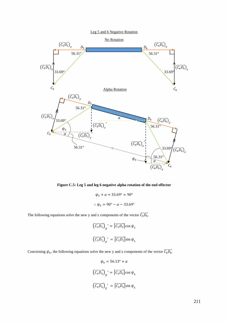
211
Figure C.5: Leg 5 and leg 6 negative alpha rotation of the end effector
𝜓5 + 𝛼 + 33.69° = 90°
∴ 𝜓5 = 90° − 𝛼 − 33.69°
The following equations solve the new y and z components of the vector 𝐶5𝐷5 .
(𝐶5𝐷5 )𝑦′ = |𝐶5𝐷5 |cos 𝜓
5
(𝐶5𝐷5 )𝑧′ = |𝐶5𝐷5 |sin 𝜓
5
Concerning 𝜓6, the following equations solve the new y and z components of the vector 𝐶6𝐷6 .
𝜓6 = 56.13° + 𝛼
(𝐶6𝐷6 )𝑦′ = |𝐶6𝐷6 |cos 𝜓
6
(𝐶6𝐷6 )𝑧′ = |𝐶6𝐷6 |sin 𝜓
6
Leg 5 and 6 Negative Rotation
No Rotation
(𝐶5𝐷5 )
𝑦
′
(𝐶5𝐷5 )
𝑧
′
(𝐶6𝐷6 )
𝑦
′
(𝐶6𝐷6 )
𝑧
′
𝛼
𝜓5
𝜓6
Alpha Rotation
(𝐶5𝐷5 )
𝑦
(𝐶5𝐷5 )
𝑧
(𝐶6𝐷6 )
𝑦
(𝐶6𝐷6 )
𝑧
56.31° 56.31°
33.69° 33.69°
(𝐶5𝐷5 )
𝑦 (𝐶6𝐷6
)𝑦
(𝐶6𝐷6 )
𝑧
𝐷5
𝐶6
𝐷6
(𝐶5𝐷5 )
𝑧
𝐶5
𝛼
𝛼
56.31°
33.69°
56.31°
56.31°
33.69°
56.31°
𝐶5
𝐷5
𝐷6
𝐶6

212
Appendix D – Quality Function Deployment
Figure D.1 to Figure D.5 illustrates excerpts of the QFD.
Figure D.1: The Legend for the QFD
Figure D.2: Relationships between the different engineering metrics

213
Figure D.3: Relationships between customer requirements and engineering metrics

214
Figure D.4: Target specifications for the engineering metrics

215
Figure D.5: Competitive analysis between industrial PKMs and the PKM developed in this study

216
Appendix E – Project Costs
Table E.1 lists the cost of components for this research.
Table E.1: Cost of components
Component Price / Unit Quantity Cost
Additive Manufacturing
Filament for additive manufactured components – eSun
1kg
R 300.00 6 R 1800.00
Magigoo Pen – bonding agent for machine bed R 600.00 1 R 600.00
Mechanical
M8 chromed linear shafts R 140.00 2 R 280.00
SK8 linear shaft support R 26.00 8 R 208.00
Linear bearings – LMK8UU R 85.00 4 R 340.00
Radial bearing – 608 ZZ R 13.00 4 R 52.00
Thrust bearings – NSK 51103 R 120.00 2 R 240.00
M8 steel threaded rod R 35.00 2 R 70.00
Aluminium flexible couplers (5mm/8mm) R 40.00 6 R 240.00
Aluminium solid couplers (5mm/8mm) R 40.00 6 R 240.00
Bolts, washers and nuts (assorted) R 250.00 R 250.00
Modular extrusions and related components
Aluminium extruded profile PG30 T – slot R 150.00 8 R 1200.00
PG30 corner brackets R 14.74 15 R 221.09
PG30 tee nuts – M5 R 4.95 60 R 297.00
Electronics
42BYGHW609 stepper motors R 240.00 4 R 960.00
42BYGHM809 stepper motors R 240.00 2 R 480.00
Arduino Mega 2560 R 250.00 1 R 250.00
24V 12.5A power supply units (Mean Well S-320-24-D) R 896.00 2 R 1792.00
TB6560 stepper motor driver R 140.00 6 R 840.00
Jumper Wires (Packs) R 30.00 2 R 60.00
Breadboard 400 PT R 22.00 2 R 44.00
5-P in-line microphone male plugs R 26.15 6 R 156.90
5-P in-line microphone female plugs R 20.85 6 R 125.10
Computer fan R 40.00 1 R 40.00
Heatshrink wire cover kit R 95.00 1 R 95.00
EasyHold plastic box (control box) – 345x310x135 R 332.00 1 R 332.00
Mains lead plug to socket R 60.00 2 R 120.00
IEC plug – male flange mounted R 7.74 2 R 15.48
Tools and equipment
Hole saw set - 16 piece R 350.00 1 R 350.00
Bosch hand drill – 750W GSB16RE R 1200.00 1 R 1200.00
Digital Vernier calliper R 285.00 1 R 285.00
Wire stripper R 150.00 1 R 150.00
Miscellaneous
Wooden platform R 68.00 1 R 68.00
TOTAL R 13401.57

217
Appendix F – Linear Actuator Concepts
F.1 Concept 1: Aluminium Sheet Concept
This concept used an aluminium sheet folded at each of its ends. One end supported a linear and radial bearing
and the other end allowed the stepper motor to be mounted. The length of the actuator could be altered by changing
the length of the aluminium sheet. This design uses wear strips to reduce the friction between the additive
manufactured slider and the aluminium sheet. The telescoping arm is an aluminium rod. An advantage of this
design is that it is lightweight and cost-effective. A disadvantage of this design is that it possessed low mechanical
rigidity. Warpage could also occur if the aluminium sheet is too thin. Figure F.1 displays the design.
Figure F.1: Linear actuator concept 1
F.2 Concept 2: Additive Manufactured Bracket Concept
This concept uses three additive manufactured brackets to link all actuator components. Instead of using an
aluminium sheet, the aluminium telescoping arm, threaded rod and aluminium guide rod increases the mechanical
rigidity of the actuator. This concept, however, requires more shaft supports and bearings. The length of the
actuator can be altered by the length of the threaded rod and guide rod. The advantage of this concept is that it
more rigid than Concept 1 and the telescoping arm has two supports. The disadvantage is that the additional
aluminium guide rod and the additional bearings make this concept heavier and more expensive. Figure F.2 shows
the design concept.
Figure F.2: Linear actuator concept 2
NEMA 17
stepper motor
Aluminum
sheet
Coupling
Wear strips Radial
bearing
Aluminum
rod
Linear bearing
Shaft support
Additive
manufactured slider Threaded rod
Additive
manufactured
bracket 1
Aluminum guide rod
Shaft support
Flexible
coupling
Linear bearing
Threaded
rod
Linear
bearing
NEMA 17
Stepper Motor
Additive manufactured bracket 2
Additive manufactured
bracket 3
Telescoping
arm

218
F.3 Concept 3: Additive Manufactured Casing with Guides and Slots
Concept 3, illustrated in Figure F.3, makes use of AM for the majority of the design. The design aimed to be
compact, lightweight, cost-effective and easy to manufacture. The outer casing, the telescoping arm and the
revolute joint attachments at the back and front of the actuator are designed for AM. The nut is fixed to the bottom
of the telescoping arm and the threaded rod rotates within the nut which causes the linear displacement of the
telescoping arm. The square-shaped design restricts the relative rotation between the telescoping arm and the outer
casing. This was aided by the guides of the outer casing and the slots on the telescoping arm. The guides and slots
were designed for two sides of the outer casing and telescoping arm.
The disadvantage of the design is that the telescoping arm is only supported by the contact between the nut and
threaded rod. The outer casing, motor and motor backplate are all held together with M3 threaded rods which run
through the length of the motor body. An M8 threaded rod is used as the lead screw and a flexible coupler attaches
the motor shaft to the M8 threaded rod.
Figure F.3: Linear actuator concept 3
F.4 Linear Actuator Pugh Selection Matrix
Table F.1 displays the criteria and the scores of each of the concepts. Concept 4 was selected.
Table F.1: Linear actuator selection matrix
Aspect Relative importance
(1-5)
Concepts
1 (Baseline) 2 3 4
Compact 4 0 -1 1 1
Cost Effective 5 0 -1 1 1
Lightweight 3 0 -1 1 1
Easy to manufacture 3 0 1 0 0
Rigidity 5 0 1 0 1
Easy to assemble 2 0 1 0 0
Good accuracy 4 0 1 1 1
Easy to interface with joints 3 0 0 1 1
Total 0 2 19 24
Motor back
plate
Outer casing Telescoping
arm Slots Guides
Stepper motor Revolute joint

219
Appendix G – PKM DOFs
G.1 Alpha Rotation
Figure G.1a depicts the isometric view of the PKM in its maximum alpha tilt pose. Figure G.1b depicts the front
view of the PKM performing the maximum alpha tilt pose. For this condition to occur, leg 2 is closed and leg 4
and leg 6 are at a maximum stroke length. The maximum tilt angled observed is 35.73°. The minimum alpha
rotation is a reflection across its x-axis; therefore, the minimum tilt angle is -35.73°. This condition occurs when
leg 4 is fully retracted and leg 2 and leg 5 are fully extended.
Figure G.1: Maximum alpha rotation
a. Isometric view of the pose for maximum alpha rotation.
b. Front view of the pose for maximum alpha rotation.
G.2 Beta Rotation
Figure G.2 shows the different views of the pose when performing the minimum beta rotation. For this pose to
occur, leg 5 and leg 6 are fully extended and parallel whilst leg 2 and leg 4 are fully retracted. The bottom corners
of the joint D brackets are 1 mm apart. The angle of the tilt observed is -36.8°.
Figure G.2: Minimum beta rotation
a. Side view of the pose for minimum beta rotation.
b. Front view of the pose for minimum beta rotation.
a. b.
a. b.

220
The maximum beta tilt angle was 27.17° as depicted in Figure G.3. In this pose, leg 5 and leg 6 are fully retracted
and leg 2 and leg 4 are fully extended. Part 2 of joint C of leg 1 and leg 2 actuator casing are 1mm apart. Part 2 of
joint C of leg 3 and the actuator casing of leg 4 are 1 mm apart as shown in Figure G.3c.
Figure G.3: Maximum beta rotation
a. Side view of the pose for maximum beta rotation.
b. Front view of the pose for maximum beta rotation.
c. Close-up view of the pose for maximum beta rotation depicting the 1 mm clash clearance between leg 3
and 4.
c.
a. b.

221
G.3 Parasitic Gamma Rotation
Parasitic motion (rotation) only occurred when the PKM performed alpha and beta rotations simultaneously.
Figure G.4a depicts an example of parasitic motion where a gamma rotation of -8.02° is induced when 𝛼 = 35.83°
and 𝛽 = -7.36°. Figure G.4b and Figure G.4c depicts the front and side views respectively which exhibits 5
independent motions and 1 parasitic motion.
Figure G.4: Existence of parasitic motion
a. Close-up view of the end effector in relation to the Joint 𝐵 bracket variation 2 illustrating parasitic
rotation.
b. Front view pose exhibiting 5 independent motions and 1 parasitic motion.
c. Side view pose exhibiting 5 independent motions and 1 parasitic motion.
a.
b. c.
-8.02°

222
G.4 Translation along x, y and z Axes
Figure G.5a depicts the translation along the positive x-axis. Figure G.5b illustrates the translation along the
positive y-axis and Figure G.5c depicts the translation of the end effector along the positive z-axis. Figure G.5
illustrates translation without any rotation of the end effector.
Figure G.5: Translation along the different axes
a. Translation along the x-axis.
b. Translation along the y-axis.
c. Translation along the z-axis.
a. b.
c.

223
Appendix H – Engineering Drawings

FRONT VIEW LEFT VIEW
ISOMETRIC VIEWSCALE 1:10
UNIVERSITY OF KWAZULU-NATAL
SCHOOL OF ENGINEERING
MECHANICAL ENGINEERING
MAT.:
PROJECT SUPERVISOR
WORKSHOP TECHNICIAN
TECHNICAL OFFICER
DATE
No. REQ.:
CHECKED
SCALE:
STUDENT NAME:
STUDENT No.:
E-MAIL:
TEL. No.:
UNITS: PROJECT:
TITLE:
No.:
0.250.25
N/A 1 1:5WESLEY DHARMALINGUM209516218
PKM
ASSEMBLY DRAWING
1 / 28mm
UNLESS OTHERWISESTATED GENERALTOLERANCES : ANGLES :
mm
SOLIDWORKS Educational Product. For Instructional Use Only.

UNIVERSITY OF KWAZULU-NATAL
SCHOOL OF ENGINEERING
MECHANICAL ENGINEERING
MAT.:
PROJECT SUPERVISOR
WORKSHOP TECHNICIAN
TECHNICAL OFFICER
DATE
No. REQ.:
CHECKED
SCALE:
STUDENT NAME:
STUDENT No.:
E-MAIL:
TEL. No.:
UNITS: PROJECT:
TITLE:
No.:
0.250.25
N/A 1 1:5WESLEY DHARMALINGUM209516218
PKM WITH TESTING FRAME AND SENSORS
ASSEMBLY DRAWING
2 / 28mm
UNLESS OTHERWISESTATED GENERALTOLERANCES : ANGLES :
mm
SOLIDWORKS Educational Product. For Instructional Use Only.
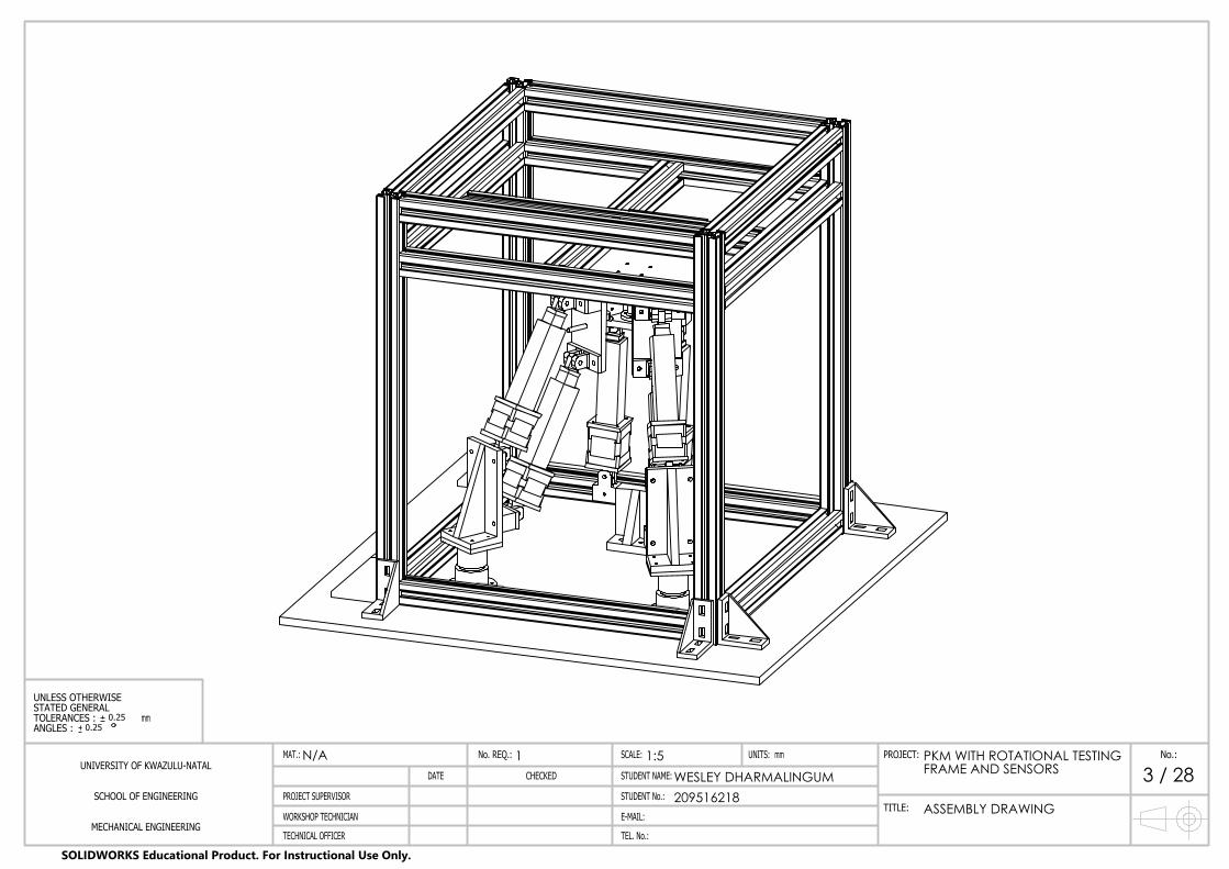
UNIVERSITY OF KWAZULU-NATAL
SCHOOL OF ENGINEERING
MECHANICAL ENGINEERING
MAT.:
PROJECT SUPERVISOR
WORKSHOP TECHNICIAN
TECHNICAL OFFICER
DATE
No. REQ.:
CHECKED
SCALE:
STUDENT NAME:
STUDENT No.:
E-MAIL:
TEL. No.:
UNITS: PROJECT:
TITLE:
No.:
0.250.25
N/A 1 1:5WESLEY DHARMALINGUM209516218
PKM WITH ROTATIONAL TESTING FRAME AND SENSORS
ASSEMBLY DRAWING
3 / 28mm
UNLESS OTHERWISESTATED GENERALTOLERANCES : ANGLES :
mm
SOLIDWORKS Educational Product. For Instructional Use Only.

5
3
7
10
1
9
4
8
2
6
ITEM NO. PART NUMBER MATERIAL QTY.
1 nema_17_39mm N/A 12 Telescoping arm PLA PLASTIC 1
3 Flexible Coupler ALUMINIUM 1
4 Actuator outer casing PLA PLASTIC 1
5 Threaded rod STEEL 16 Joint C part 2 PLA PLASTIC 1
7 Joint B part 2 PLA PLASTIC 1
8 ISO - 4032 - M8 - W - N STEEL 1
9 M3 threaded rod STEEL 4
10 ISO - 4035 - M3 - N STEEL 8
UNIVERSITY OF KWAZULU-NATAL
SCHOOL OF ENGINEERING
MECHANICAL ENGINEERING
MAT.:
PROJECT SUPERVISOR
WORKSHOP TECHNICIAN
TECHNICAL OFFICER
DATE
No. REQ.:
CHECKED
SCALE:
STUDENT NAME:
STUDENT No.:
E-MAIL:
TEL. No.:
UNITS: PROJECT:
TITLE:
No.:
0.250.25
N/A 6 1:2WESLEY DHARMALINGUM209516218
LINEAR ACTUATOR
EXPLODED VIEW
4 / 28mm
UNLESS OTHERWISESTATED GENERALTOLERANCES : ANGLES :
mm
SOLIDWORKS Educational Product. For Instructional Use Only.

2
5
4
3
1
6
ITEM NO. PART NUMBER MATERIAL QTY.
1 thrust bearing bottom bracket PLA PLASTIC 1
2 Radial bearing STEEL 2
3 Thrust bearing bottom STEEL 1
4 Thrust bearing middle STEEL 1
5 Thrust bearing top STEEL 1
6 thrust bearing top bracket PLA PLASTIC 1
UNIVERSITY OF KWAZULU-NATAL
SCHOOL OF ENGINEERING
MECHANICAL ENGINEERING
MAT.:
PROJECT SUPERVISOR
WORKSHOP TECHNICIAN
TECHNICAL OFFICER
DATE
No. REQ.:
CHECKED
SCALE:
STUDENT NAME:
STUDENT No.:
E-MAIL:
TEL. No.:
UNITS: PROJECT:
TITLE:
No.:
0.250.25
N/A 2 1:1WESLEY DHARMALINGUM209516218
THRUST BEARING JOINT
EXPLODED VIEW
5 / 28mm
UNLESS OTHERWISESTATED GENERALTOLERANCES : ANGLES :
mm
SOLIDWORKS Educational Product. For Instructional Use Only.

AA
SECTION A-ASCALE 1 : 1
8 2 10 4
79135
6
ITEM NO. PART NUMBER
1 nema_17_39mm2 Telescoping arm
3 Flexible Coupler
4 Actuator outer casing
5 Threaded rod6 Joint C part 2
7 Joint B part 2
8 ISO - 4032 - M8 - W - N
9 M3 threaded rod
10 ISO - 4035 - M3 - N
UNIVERSITY OF KWAZULU-NATAL
SCHOOL OF ENGINEERING
MECHANICAL ENGINEERING
MAT.:
PROJECT SUPERVISOR
WORKSHOP TECHNICIAN
TECHNICAL OFFICER
DATE
No. REQ.:
CHECKED
SCALE:
STUDENT NAME:
STUDENT No.:
E-MAIL:
TEL. No.:
UNITS: PROJECT:
TITLE:
No.:
0.250.25
N/A 6 1:1WESLEY DHARMALINGUM209516218
LINEAR ACTUATOR
SECTIONED VIEW
6 / 28mm
UNLESS OTHERWISESTATED GENERALTOLERANCES : ANGLES :
mm
SOLIDWORKS Educational Product. For Instructional Use Only.

42,05
42,
05
26,20
4x holes
3,00
8,0
5
30,
25
34,
25
18,20
32,
25
5,00
110,00
UNIVERSITY OF KWAZULU-NATAL
SCHOOL OF ENGINEERING
MECHANICAL ENGINEERING
MAT.:
PROJECT SUPERVISOR
WORKSHOP TECHNICIAN
TECHNICAL OFFICER
DATE
No. REQ.:
CHECKED
SCALE:
STUDENT NAME:
STUDENT No.:
E-MAIL:
TEL. No.:
UNITS: PROJECT:
TITLE:
No.:
0.250.25
PLA PLASTIC 6 1:1WESLEY DHARMALINGUM209516218
ACTUATOR OUTER CASING
DETAILED DRAWING
7 / 28mm
UNLESS OTHERWISESTATED GENERALTOLERANCES : ANGLES :
mm
SOLIDWORKS Educational Product. For Instructional Use Only.
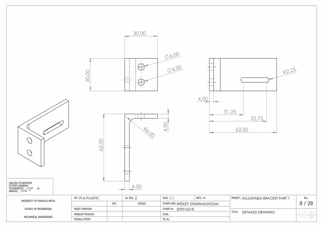
30,00
30,
00
6,00
6,00
4,00
31,25 52,75
62,00
R2,25
62,
00
4,00
4,0
0
R6,00
UNIVERSITY OF KWAZULU-NATAL
SCHOOL OF ENGINEERING
MECHANICAL ENGINEERING
MAT.:
PROJECT SUPERVISOR
WORKSHOP TECHNICIAN
TECHNICAL OFFICER
DATE
No. REQ.:
CHECKED
SCALE:
STUDENT NAME:
STUDENT No.:
E-MAIL:
TEL. No.:
UNITS: PROJECT:
TITLE:
No.:
0.250.25
PLA PLASTIC 2 1:1WESLEY DHARMALINGUM209516218
ADJUSTABLE BRACKET PART 1
DETAILED DRAWING
8 / 28mm
UNLESS OTHERWISESTATED GENERALTOLERANCES : ANGLES :
mm

15,00 65,00
80,00
10,
00
20,
00
4,0
0
4,0
0 34,00
16,00
26,00
4,0
0
4,00
R8,00
4,00
34,
00
4,0
0
UNIVERSITY OF KWAZULU-NATAL
SCHOOL OF ENGINEERING
MECHANICAL ENGINEERING
MAT.:
PROJECT SUPERVISOR
WORKSHOP TECHNICIAN
TECHNICAL OFFICER
DATE
No. REQ.:
CHECKED
SCALE:
STUDENT NAME:
STUDENT No.:
E-MAIL:
TEL. No.:
UNITS: PROJECT:
TITLE:
No.:
0.250.25
PLA PLASTIC 2 1:1WESLEY DHARMALINGUM209516218
ADJUSTABLE BRACKET PART 2
DETAILED DRAWING
9 / 28mm
UNLESS OTHERWISESTATED GENERALTOLERANCES : ANGLES :
mm

259,81
259,81
259
,81
210
,00
235
,00
260
,00
297,50
310,00
322,50
460
,00
180,10
4 HOLES ON A 50mm DIAMETER
4 HOLES ON A 50mm DIAMETER
ALL HOLES HAVE A DIAMETER OF 4 mm
THE THICKNESS OF THE BASE IS 10 mm
UNIVERSITY OF KWAZULU-NATAL
SCHOOL OF ENGINEERING
MECHANICAL ENGINEERING
MAT.:
PROJECT SUPERVISOR
WORKSHOP TECHNICIAN
TECHNICAL OFFICER
DATE
No. REQ.:
CHECKED
SCALE:
STUDENT NAME:
STUDENT No.:
E-MAIL:
TEL. No.:
UNITS: PROJECT:
TITLE:
No.:
0.250.25
PLA PLASTIC 1 1:5WESLEY DHARMALINGUM209516218
BASE
DETAILED DRAWING
10 / 28mm
UNLESS OTHERWISESTATED GENERALTOLERANCES : ANGLES :
mm

33,
00
8,29 11,72
28,30 31,70
48,30 51,70
68,30 71,70 88,30 91,70
14,
20
15,
80
33,
00
20,00 80,00
18,
00
6,00 6,00
R8,00
3,00
33,00
UNIVERSITY OF KWAZULU-NATAL
SCHOOL OF ENGINEERING
MECHANICAL ENGINEERING
MAT.:
PROJECT SUPERVISOR
WORKSHOP TECHNICIAN
TECHNICAL OFFICER
DATE
No. REQ.:
CHECKED
SCALE:
STUDENT NAME:
STUDENT No.:
E-MAIL:
TEL. No.:
UNITS: PROJECT:
TITLE:
No.:
0.250.25
PLA PLASTIC 2 1:1WESLEY DHARMALINGUM209516218
DEPTH MEASURING BRACKET
DETAILED DRAWING
11 / 28mm
UNLESS OTHERWISESTATED GENERALTOLERANCES : ANGLES :
mm

2x holes 5,00
R6,50
R12,00
4x holes 3,00
56,39
11,
09
23,
09
35,
09
13,00 25,00
37,00 1
20°
20,00
20,
00
12,00
51,
78
20,
00
6,0
0
6,1
0
13,
90
14,
00
50,00 ALL HOLES AROUND THECENTRE OF THE END EFFECTOR HAS A 3 mmDIAMETER
UNIVERSITY OF KWAZULU-NATAL
SCHOOL OF ENGINEERING
MECHANICAL ENGINEERING
MAT.:
PROJECT SUPERVISOR
WORKSHOP TECHNICIAN
TECHNICAL OFFICER
DATE
No. REQ.:
CHECKED
SCALE:
STUDENT NAME:
STUDENT No.:
E-MAIL:
TEL. No.:
UNITS: PROJECT:
TITLE:
No.:
0.250.25
PLA PLASTIC 1 1:1WESLEY DHARMALINGUM209516218
END EFFECTOR
DETAILED DRAWING
12 / 28mm
UNLESS OTHERWISESTATED GENERALTOLERANCES : ANGLES :
mm
SOLIDWORKS Educational Product. For Instructional Use Only.

5,0
0
8,00
R2,00
22,
00
60,00
8,00 8,00
2x holes 5,00
18,00 34,00
3,0
0 19,
00
R5,00
R2,00
5,00
UNIVERSITY OF KWAZULU-NATAL
SCHOOL OF ENGINEERING
MECHANICAL ENGINEERING
MAT.:
PROJECT SUPERVISOR
WORKSHOP TECHNICIAN
TECHNICAL OFFICER
DATE
No. REQ.:
CHECKED
SCALE:
STUDENT NAME:
STUDENT No.:
E-MAIL:
TEL. No.:
UNITS: PROJECT:
TITLE:
No.:
0.250.25
PLA PLASTIC 8 2 : 1WESLEY DHARMALINGUM209516218
JOINT B AND C VARIATION 1PART 1
DETAILED DRAWING
13 / 28mm
UNLESS OTHERWISESTATED GENERALTOLERANCES : ANGLES :
mm
SOLIDWORKS Educational Product. For Instructional Use Only.

6,00 14,00
20,00
20,
08 1
5,00
30,
00
5,0
0
15,
00
40,00
3,90
10,00
16,10
20,00
32,50
3,00
5,
00
R2,00 R5,00
40,
00
12
,20
10,
00
10,00
20,
00
UNIVERSITY OF KWAZULU-NATAL
SCHOOL OF ENGINEERING
MECHANICAL ENGINEERING
MAT.:
PROJECT SUPERVISOR
WORKSHOP TECHNICIAN
TECHNICAL OFFICER
DATE
No. REQ.:
CHECKED
SCALE:
STUDENT NAME:
STUDENT No.:
E-MAIL:
TEL. No.:
UNITS: PROJECT:
TITLE:
No.:
0.250.25
PLA PLASTIC 4 2:1WESLEY DHARMALINGUM209516218
JOINT B AND C VARIATION 2 PART 1
DETAILED DRAWING
14 / 28mm
UNLESS OTHERWISESTATED GENERALTOLERANCES : ANGLES :
mm
SOLIDWORKS Educational Product. For Instructional Use Only.

48,
00
4x holes 3,00
16,
00 4
0,00
7,93 51,93
118
,00
4x holes 5,00
25,00 35,00
60,00 8,00
UNIVERSITY OF KWAZULU-NATAL
SCHOOL OF ENGINEERING
MECHANICAL ENGINEERING
MAT.:
PROJECT SUPERVISOR
WORKSHOP TECHNICIAN
TECHNICAL OFFICER
DATE
No. REQ.:
CHECKED
SCALE:
STUDENT NAME:
STUDENT No.:
E-MAIL:
TEL. No.:
UNITS: PROJECT:
TITLE:
No.:
0.250.25
PLA PLASTIC 2 1 : 1.25WESLEY DHARMALINGUM209516218
JOINT B BRACKET VARIATION 1
DETAILED DRAWING
15 / 28mm
UNLESS OTHERWISESTATED GENERALTOLERANCES : ANGLES :
mm
SOLIDWORKS Educational Product. For Instructional Use Only.

116,57°
12,00
20,00
10,
00 5
4,00
60,
00
70,
00
20,
00
30,
00
50,
00
12,
50
37,
50
4x holes 5,00
15,00
65,00 40,00
UNIVERSITY OF KWAZULU-NATAL
SCHOOL OF ENGINEERING
MECHANICAL ENGINEERING
MAT.:
PROJECT SUPERVISOR
WORKSHOP TECHNICIAN
TECHNICAL OFFICER
DATE
No. REQ.:
CHECKED
SCALE:
STUDENT NAME:
STUDENT No.:
E-MAIL:
TEL. No.:
UNITS: PROJECT:
TITLE:
No.:
0.250.25
PLA PLASTIC 1 1:1WESLEY DHARMALINGUM209516218
JOINT B BRACKET VARIATION 2
DETAILED DRAWING
16 / 28mm
UNLESS OTHERWISESTATED GENERALTOLERANCES : ANGLES :
mm
SOLIDWORKS Educational Product. For Instructional Use Only.

42,30
7,60
20,
00
42,
30
42,30
4x holes 3,00
5,0
0
5,00
UNIVERSITY OF KWAZULU-NATAL
SCHOOL OF ENGINEERING
MECHANICAL ENGINEERING
MAT.:
PROJECT SUPERVISOR
WORKSHOP TECHNICIAN
TECHNICAL OFFICER
DATE
No. REQ.:
CHECKED
SCALE:
STUDENT NAME:
STUDENT No.:
E-MAIL:
TEL. No.:
UNITS: PROJECT:
TITLE:
No.:
0.250.25
PLA PLASTIC 6 1:1WESLEY DHARMALINGUM209516218
JOINT B PART 2
DETAILED DRAWING
17 / 28mm
UNLESS OTHERWISESTATED GENERALTOLERANCES : ANGLES :
mm
SOLIDWORKS Educational Product. For Instructional Use Only.

25,
00
5,0
0
6,6
7
17,
50
7,60
R2,00
5,00
R2,00
R5,00
17,
80
17,80
16,
00
UNIVERSITY OF KWAZULU-NATAL
SCHOOL OF ENGINEERING
MECHANICAL ENGINEERING
MAT.:
PROJECT SUPERVISOR
WORKSHOP TECHNICIAN
TECHNICAL OFFICER
DATE
No. REQ.:
CHECKED
SCALE:
STUDENT NAME:
STUDENT No.:
E-MAIL:
TEL. No.:
UNITS: PROJECT:
TITLE:
No.:
0.250.25
PLA PLASTIC 6 2:1WESLEY DHARMALINGUM209516218
JOINT C PART 2
DETAILED DRAWING
18 / 28mm
UNLESS OTHERWISESTATED GENERALTOLERANCES : ANGLES :
mm
SOLIDWORKS Educational Product. For Instructional Use Only.

102
,00
60,00
11,
00
51,
00
91,
00
7,50
52,50
5x holes 5,00 8,00
UNIVERSITY OF KWAZULU-NATAL
SCHOOL OF ENGINEERING
MECHANICAL ENGINEERING
MAT.:
PROJECT SUPERVISOR
WORKSHOP TECHNICIAN
TECHNICAL OFFICER
DATE
No. REQ.:
CHECKED
SCALE:
STUDENT NAME:
STUDENT No.:
E-MAIL:
TEL. No.:
UNITS: PROJECT:
TITLE:
No.:
0.250.25
PLA PLASTIC 2 1:1WESLEY DHARMALINGUM209516218
JOINT D BRACKET
DETAILED DRAWING
19 / 28mm
UNLESS OTHERWISESTATED GENERALTOLERANCES : ANGLES :
mm
SOLIDWORKS Educational Product. For Instructional Use Only.

36,00
5,00
20,
00
7,90 7,90 R2,00
5,
00
16,
00
R2,00
5,0
0
7,0
0
20,
00
25,
00
8,20
17,
50
UNIVERSITY OF KWAZULU-NATAL
SCHOOL OF ENGINEERING
MECHANICAL ENGINEERING
MAT.:
PROJECT SUPERVISOR
WORKSHOP TECHNICIAN
TECHNICAL OFFICER
DATE
No. REQ.:
CHECKED
SCALE:
STUDENT NAME:
STUDENT No.:
E-MAIL:
TEL. No.:
UNITS: PROJECT:
TITLE:
No.:
0.250.25
PLA PLASTIC 2 2:1WESLEY DHARMALINGUM209516218
JOINT D FORKED ATTACHMENT
DETAILED DRAWING
20 / 28mm
UNLESS OTHERWISESTATED GENERALTOLERANCES : ANGLES :
mm
SOLIDWORKS Educational Product. For Instructional Use Only.

10,
00 1
3,00
25,
00
37,
00
40,
00
10,00
13,00 25,00 40,00
4x holes 4,00
4x holes 3,00
33,00
20
,00
11
,00
4,0
0
54,
00
58,
00
17,00
33,00
R2,00
UNIVERSITY OF KWAZULU-NATAL
SCHOOL OF ENGINEERING
MECHANICAL ENGINEERING
MAT.:
PROJECT SUPERVISOR
WORKSHOP TECHNICIAN
TECHNICAL OFFICER
DATE
No. REQ.:
CHECKED
SCALE:
STUDENT NAME:
STUDENT No.:
E-MAIL:
TEL. No.:
UNITS: PROJECT:
TITLE:
No.:
0.250.25
PLA PLASTIC 1 1:1WESLEY DHARMALINGUM209516218
MIRROR MOUNTING BRACKET
DETAILED DESIGN
21 / 28mm
UNLESS OTHERWISESTATED GENERALTOLERANCES : ANGLES :
mm
SOLIDWORKS Educational Product. For Instructional Use Only.

31,00 42,00
73,00
15,
00
30,
00
3,0
0
11,
00
8,0
0
9,1
5
13,
50
14,
94
R2,00
18,
00
28,
00
21,
00
28,
00
37,
00
46,
00
49,
00
38,
00
40,
45
6,00 43,00 56,00
7,30 13,00 41,00
54,00 59,00
69,00
3,00
46,00 49,00
30,
00
2,0
0
5,0
0
21,00 28,00
UNIVERSITY OF KWAZULU-NATAL
SCHOOL OF ENGINEERING
MECHANICAL ENGINEERING
MAT.:
PROJECT SUPERVISOR
WORKSHOP TECHNICIAN
TECHNICAL OFFICER
DATE
No. REQ.:
CHECKED
SCALE:
STUDENT NAME:
STUDENT No.:
E-MAIL:
TEL. No.:
UNITS: PROJECT:
TITLE:
No.:
0.250.25
PLA PLASTIC 2 1:1WESLEY DHARMALINGUM209516218
OCM SENSOR HOUSING PART 1
DETAILED DRAWING
22 / 28mm
UNLESS OTHERWISESTATED GENERALTOLERANCES : ANGLES :
mm
SOLIDWORKS Educational Product. For Instructional Use Only.

60,00
22,
00
2x holes 5,00
20,00
ISOMETRIC VIEWSCALE 1:1
UNIVERSITY OF KWAZULU-NATAL
SCHOOL OF ENGINEERING
MECHANICAL ENGINEERING
MAT.:
PROJECT SUPERVISOR
WORKSHOP TECHNICIAN
TECHNICAL OFFICER
DATE
No. REQ.:
CHECKED
SCALE:
STUDENT NAME:
STUDENT No.:
E-MAIL:
TEL. No.:
UNITS: PROJECT:
TITLE:
No.:
0.250.25
PLA PLASTIC 4 2:1WESLEY DHARMALINGUM209516218
SPACER
DETAILED DRAWING
23 / 28mm
UNLESS OTHERWISESTATED GENERALTOLERANCES : ANGLES :
mm
SOLIDWORKS Educational Product. For Instructional Use Only.

72,
00
66,
00
21,80
21,
80
2,0
0
19,
80
7,62
13,
20
10
,00
UNIVERSITY OF KWAZULU-NATAL
SCHOOL OF ENGINEERING
MECHANICAL ENGINEERING
MAT.:
PROJECT SUPERVISOR
WORKSHOP TECHNICIAN
TECHNICAL OFFICER
DATE
No. REQ.:
CHECKED
SCALE:
STUDENT NAME:
STUDENT No.:
E-MAIL:
TEL. No.:
UNITS: PROJECT:
TITLE:
No.:
0.250.25
PLA PLASTIC 6 1:1WESLEY DHARMALINGUM209516218
TELESCOPING ARM
DETAILED DRAWING
24 / 28mm
UNLESS OTHERWISESTATED GENERALTOLERANCES : ANGLES :
mm
SOLIDWORKS Educational Product. For Instructional Use Only.

5,0
0 2
7,00
4,00
60
,00
40
,00
30
,20
30
,00
22
,20
8,
00
UNIVERSITY OF KWAZULU-NATAL
SCHOOL OF ENGINEERING
MECHANICAL ENGINEERING
MAT.:
PROJECT SUPERVISOR
WORKSHOP TECHNICIAN
TECHNICAL OFFICER
DATE
No. REQ.:
CHECKED
SCALE:
STUDENT NAME:
STUDENT No.:
E-MAIL:
TEL. No.:
UNITS: PROJECT:
TITLE:
No.:
0.250.25
PLAPLASTIC 2 1:1WESLEY DHARMALINGUM209516218
THRUST BEARING BOTTOM BRACKET
DETAILED DRAWING
25 / 28mm
UNLESS OTHERWISESTATED GENERALTOLERANCES : ANGLES :
mm
SOLIDWORKS Educational Product. For Instructional Use Only.

31,
00
26,
00
48,00
60,
00
30
,20
36
,00
8,0
0
52,
00
28
,00
22
,20
8,
00
4X HOLES 3,00
8,00 32,00
UNIVERSITY OF KWAZULU-NATAL
SCHOOL OF ENGINEERING
MECHANICAL ENGINEERING
MAT.:
PROJECT SUPERVISOR
WORKSHOP TECHNICIAN
TECHNICAL OFFICER
DATE
No. REQ.:
CHECKED
SCALE:
STUDENT NAME:
STUDENT No.:
E-MAIL:
TEL. No.:
UNITS: PROJECT:
TITLE:
No.:
0.250.25
PLA PLASTIC 2 0.75 : 1WESLEY DHARMALINGUM209516218
THRUST BEARINGTOP BRACKET
DETAILED DRAWING
26 / 28mm
UNLESS OTHERWISESTATED GENERALTOLERANCES : ANGLES :
mm
SOLIDWORKS Educational Product. For Instructional Use Only.
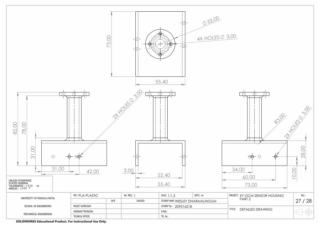
3,00 52,40
55,40
10,
00
28,
00
34,00 60,00 73,00
R3,00
2X H
OLE
S 3,
00
73,
00
55,40
33,00
4X HOLES 3,00
31,00 42,00
31,
00
78,
00
82,
00 2X
HOLES
3,00
UNIVERSITY OF KWAZULU-NATAL
SCHOOL OF ENGINEERING
MECHANICAL ENGINEERING
MAT.:
PROJECT SUPERVISOR
WORKSHOP TECHNICIAN
TECHNICAL OFFICER
DATE
No. REQ.:
CHECKED
SCALE:
STUDENT NAME:
STUDENT No.:
E-MAIL:
TEL. No.:
UNITS: PROJECT:
TITLE:
No.:
0.250.25
PLA PLASTIC 1 1:1.2WESLEY DHARMALINGUM209516218
XY OCM SENSOR HOUSING PART 2
DETAILED DRAWING
27 / 28mm
UNLESS OTHERWISESTATED GENERALTOLERANCES : ANGLES :
mm
SOLIDWORKS Educational Product. For Instructional Use Only.

3,00
52,40 55,40
28,
00
70,
00
R7,00
25,
00 63,
00
8,00 28,00
2X HOLES 5,00
34,00 60,00
73,00
10,
00
50,
00 56,
00
3,00
3,00
73,
00
13,
80 1
7,80
5
5,20
59,
20
9,70 13,70 41,70 45,70
13,80
17,80
55,20
59,20
3,00
3,00
ISOMETRIC VIEWSCALE 1:2
UNIVERSITY OF KWAZULU-NATAL
SCHOOL OF ENGINEERING
MECHANICAL ENGINEERING
MAT.:
PROJECT SUPERVISOR
WORKSHOP TECHNICIAN
TECHNICAL OFFICER
DATE
No. REQ.:
CHECKED
SCALE:
STUDENT NAME:
STUDENT No.:
E-MAIL:
TEL. No.:
UNITS: PROJECT:
TITLE:
No.:
0.250.25
PLA PLASTIC 1 1:1.4WESLEY DHARMALINGUM209516218
Z OCM SENSOR HOUSING PART 2
DETAILED DRAWING
28 / 28mm
UNLESS OTHERWISESTATED GENERALTOLERANCES : ANGLES :
mm
SOLIDWORKS Educational Product. For Instructional Use Only.